ELECTRONIC PREPRINT: P. Svec, A. Thakur, E. Raboin, B.C. Shah, S.K. Gupta.Target Following with Motion Prediction for Unmanned Surface Vehicle Operating inCluttered Environments. Autonomous Robots, Accepted for publication.

Autonomous Robots, manuscript No.(will be inserted by the editor)

Target Following with Motion Prediction for Unmanned SurfaceVehicle Operating in Cluttered Environments

Petr Svec · Atul Thakur · Eric Raboin · Brual C. Shah ·

Satyandra K. Gupta

Received: date / Accepted: date

Abstract The capability of following a moving target in

an environment with obstacles is required as a basic and

necessary function for realizing an autonomous unmannedsurface vehicle (USV). Many target following scenarios in-

volve a follower and target vehicles that may have different

maneuvering capabilities. Moreover, the follower vehicle

may not have prior information about the intended mo-tion of the target boat. This paper presents a trajectory

planning and tracking approach for following a differen-

tially constrained target vehicle operating in an obstacle

field. The developed approach includes a novel algorithm

for computing a desired pose and surge speed in the vicin-ity of the target boat, jointly defined as a motion goal, and

Petr SvecSimulation Based System Design Laboratory, Maryland RoboticsCenter, Department of Mechanical Engineering, University ofMaryland, College Park, MD 20742, USAE-mail: petrsvec@umd.edu

Atul ThakurDepartment of Mechanical Engineering, Indian Institute of Tech-nology Patna, Patliputra, Bihar, 800013, IndiaE-mail: athakur@iitp.ac.in

Eric RaboinDepartment of Computer Science, University of Maryland, Col-lege Park, MD 20742, USAE-mail: eraboin@umd.edu

Brual C. ShahSimulation Based System Design Laboratory, Department of Me-chanical Engineering, University of Maryland, College Park, MD20742, USAE-mail: brual@umd.edu

Satyandra K. GuptaSimulation Based System Design Laboratory, Maryland RoboticsCenter, Department of Mechanical Engineering and Institute forSystems Research, University of Maryland, College Park, MD20742, USAE-mail: skgupta@umd.edu

tightly integrates it with trajectory planning and tracking

components of the entire system. The trajectory planner

generates a dynamically feasible, collision-free trajectoryto allow the USV to safely reach the computed motion

goal. Trajectory planning needs to be sufficiently fast and

yet produce dynamically feasible and short trajectories due

to the moving target. This required speeding up the plan-ning by searching for trajectories through a hybrid, pose-

position state space using a multi-resolution control action

set. The search in the velocity space is decoupled from the

search for a trajectory in the pose space. Therefore, the

underlying trajectory tracking controller computes desiredsurge speed for each segment of the trajectory and ensures

that the USV maintains it. We have carried out simulation

as well as experimental studies to demonstrate the effec-

tiveness of the developed approach.

Keywords Unmanned surface vehicle (USV) · Follow

behavior · Motion prediction · Trajectory planning ·

Trajectory tracking

1 Introduction

Autonomous unmanned surface vehicles (USVs) [1,2,3,4]

can increase the capability of other surface or underwater

vehicles by continuously following them in marine appli-

cations. These include sea-bed mapping and ocean sam-pling tasks [5,6,7] in environmental monitoring [8,9,10],

cooperative surveillance by means of a network of hetero-

geneous vehicles (e.g., air, ground, and marine unmanned

platforms) to provide situational awareness [11,12,13], searchand rescue [14,15], or harbor patrolling and protecting vul-

nerable areas [16,17,18,19,20].

Consider the case of a cooperative team of USVs guard-

ing an asset against hostile boats in naval missions [20]. In

2 Petr Svec et al.

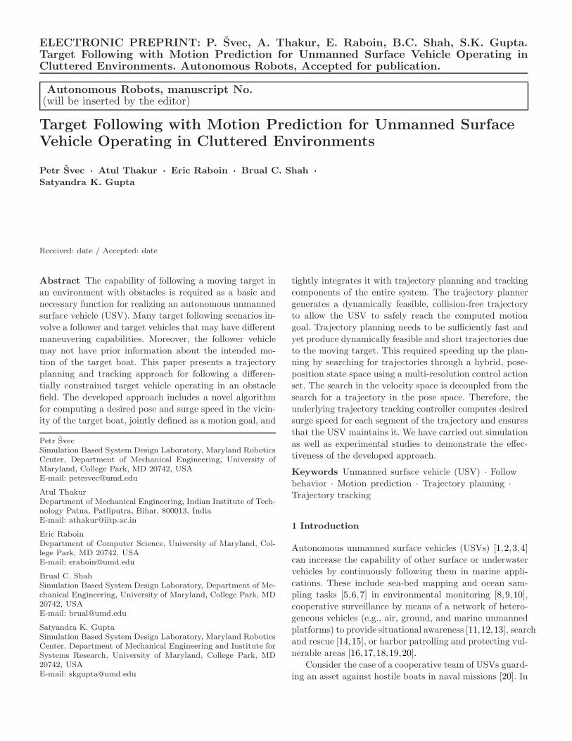
Fig. 1: A typical bay with various types of moving boats

(source: Map data c©2013 Google).

these missions, the vehicles are required to approach pass-

ing boats, recognize adversaries, and possibly employ ac-tive blocking [19] to prevent the adversaries from reaching

the asset. In order to maximize the guarding performance

of the entire team, it is necessary for each USV to consider

its own dynamics when approaching or following the boats.

Moreover, each USV should be able to reliably compute itsdesired position [x, y]T , orientation ψ, and surge speed u

values, jointly defined as a motion goal, by estimating the

future poses of the boats.

Performing autonomous follow task in an unfamiliar,

unstructured marine environment (see Figure 1) with ob-stacles of variable dimensions, shapes, and motion dynam-

ics such as other unmanned surface vehicles, civilian boats,

adversaries, shorelines, or docks poses numerous planning

challenges. The follow capability of the USV is inherently

influenced by its own maneuverability constraints, the spe-cific motion characteristics of the target boat, the amount

of knowledge about the intended motion of the target boat,

sensing limitations, and the complexity of the marine envi-

ronment. Due to differences in motion capabilities with re-spect to the target boat, the USV may not be able to track

the same trajectory as the target boat. Instead, it may need

to determine a different trajectory to follow, while keeping

itself in proximity to the target boat and still avoid colli-

sions. In addition, the USV may need to handle sharp turnswhile tracking the trajectory. Therefore, the mere utiliza-

tion of manually developed and tuned control rules would

not lead to sufficiently safe and task efficient follow strate-

gies in environments with obstacles. In order to cope withthe above outlined challenges, the USV needs to have a)

the capability to estimate the future motion of the target

boat based on its current state, dynamic characteristics, as

well as obstacles in the operating environment, b) the capa-

bility to determine an advantageous and safe pose, i.e., in

the form of a motion goal, in the close vicinity to the targetboat, and c) fast, dynamically feasible trajectory planning

and reliable trajectory tracking to guarantee physics-aware

obstacle avoidance when approaching the motion goal.

We have developed a planning and tracking approach

that incorporates a novel algorithm for motion goal com-putation, and tightly integrates it with trajectory planning

and tracking components of the entire system to perform

integrated planning and control. The motion goal is com-

puted based on differential constraints of the USV and thetarget boat, expected motion of the target that is com-

puted using a probability distribution over its possible con-

trol actions, and spatial constraints imposed by the envi-

ronment. In particular, it forward-projects the control ac-

tions of the target boat to estimate a probability distribu-tion of its future pose, computes candidate motion goals,

selects the motion goal that minimizes the difference be-

tween the arrival time of the USV and the target boat

to that goal, and attempts to minimize the length of theUSV’s trajectory.

The developed trajectory planner incorporates A* based

heuristic search [21] to efficiently find a collision-free, dy-

namically feasible trajectory to a motion goal in a dis-

cretized state-action space, forming a lattice [22]. The tra-jectory is computed by sequencing predefined control ac-

tions (i.e., maneuvers or motion primitives) generated us-

ing the dynamics model of the USV [23,24]. The trajectory

is executed by a trajectory tracking controller to efficiently

follow waypoints that make up the nominal trajectory. Thecontroller computes the desired speed for each segment of

the trajectory given the maximum allowable surge speed

of the segment. This allows the USV to arrive to the mo-

tion goal at the required time. We have carried out exper-imental tests to determine the required acceleration and

deceleration distance for the vehicle to match the desired

speed.

In general, one can assume that the USV is capable of

rejecting ocean disturbances in low sea states due to itsmechanical design and the use of feedback based position

control including roll stabilization [24]. However, this as-

sumption may not be valid in higher sea states. Therefore,

we determine collision zones around obstacles by comput-ing the region of inevitable collision [25] and replan the

trajectory with a high frequency to account for the uncer-

tainty in the vehicle’s motion. In addition, we assume that

the combined set of sensors (e.g., lidar, stereo cameras, and

radar), digital nautical charts, and Kalman filtering [26]will provide us reasonable state estimation of obstacles as

well as the USV.

Since the target boat may be moving with a high speed,

the trajectory needs to be computed sufficiently fast and

Target Following with Motion Prediction for Unmanned Surface Vehicle Operating in Cluttered Environments 3

still preserve its dynamical feasibility in the close vicinity

to the USV. The quality of the computed trajectory as wellas the computational performance of the planner depends

on the number and type of control actions and dimension-

ality of the underlying state space in different planning

stages. A high-quality trajectory may be close to optimumin terms of its execution time but may take a long time

to be computed on a given machine. On the other hand, a

low-quality trajectory will be computed very quickly but

may be longer with unnecessary detours. Both the cases

would thus lead to a poor overall follow capability. Hence,it was necessary to sacrifice allowable level of optimality

by superimposing high and low dimensional state spaces

and utilizing a multi-resolution control action set. In par-

ticular, the dimensionality of the state space as well as thenumber of control actions is reduced with the increase of

the distance from the USV towards the target. We have

conducted a detailed empirical analysis to find a trade-off

between fast computation and trajectory length.

This paper builds on our previous work [27], where weintroduced a lattice-based planner for computation of a

dynamically feasible, collision-free trajectory for the USV

to approach a dynamically moving motion goal. We present

the following new results:

1. We have developed a novel algorithm for motion goalprediction that has the capability of estimating the fu-

ture pose of the target boat with increased precision.

This is possible through the utilization of known target

boat’s dynamics as well as its action selection modelthat defines a probability distribution over the target’s

control actions.

2. We have carried out a detailed empirical analysis of

the effect of varying state space dimension and control

action set resolution on the computational efficiency ofthe planner and trajectory length.

3. We have improved the trajectory tracking technique

that computes the desired speed for each segment of the

trajectory, given the required arrival time to the motiongoal and upper bounds on the speed of its individual

segments.

4. We have carried out physical experiments using radio

controlled boats to evaluate the developed planner in a

real world scenario.

The outline of the paper is as follows. First, we re-

view existing major planning and control approaches in

Section 2. Second, we present the definition of the problem

in Section 3, followed by an overview of the overall ap-proach in Section 4. This overview includes a description

of the developed USV system architecture (see Figure 2)

that integrates all planning modules. Next, we describe

the state-action space representation that is used in both

motion goal prediction in Section 6 as well as in nominal

trajectory planning in Section 7.1. This is followed by adescription of the developed trajectory tracking technique

in Section 7.2. Finally, we present simulation as well as

experimental results in Section 8.

2 Literature Review

Here, we will provide a review of representative works re-

lated to following a moving target boat in an environment

with obstacles. Our particular focus is on reviewing tech-

niques for following a moving target that does not neces-sarily attempt to evade. Readers interested in the pursuit

and evasion problems can refer to a comprehensive survey

in [28]. This review includes techniques for target follow-

ing, control and guidance systems in the USV domain, aswell as trajectory planning techniques for vehicles with dif-

ferential constraints.

2.1 Target Following

A survey of state-of-the-art approaches for target follow-ing can be found in [29]. This includes multi-vehicle motion

control. In addition, the paper presents experimental val-

idation of USV following a leader vessel by observing its

path and precisely executing it using a path-following al-

gorithm. The experiments were demonstrated on ALANISand Charlie platforms.

High-speed straight-line tracking capability was devel-

oped in [30] to allow underactuated USV follow a movingtarget. Based on the guidance system previously utilized

for interceptor missiles, the motion control system is com-

posed of constant bearing guidance and velocity control

schema that allows high and precise maneuverability.

A variety of advanced maneuvers for searching and track-

ing a target, docking, reactive collision avoidance, U-turn,

course tracking, and waypoint following are implemented

on the MESSIN system [12]. The system is capable of han-dling failures of its components through various emergency

programs. In addition, the integrated path planning uti-

lizes waypoints and motion primitives represented as cir-

cular arcs.

Cooperative control [5] is an extension to the basic

follow behavior using which multiple unmanned vehicles

can track their corresponding paths while keeping them-

selves in a formation and maintaining the required speedto track the target. In this work, path and target follow-

ing primitives were evaluated using physical Aguas Vivas

and DELFIMX USV platforms. In addition, simulation re-

sults generated using NetMarSyS simulator were presented

4 Petr Svec et al.

where three USVs followed their paths in a marine envi-

ronment with ocean currents. The aim of the proposed so-lution was also to cope with communication uncertainties

between surface and underwater vehicles during the follow

task. Another multi-vehicle follow experiment on real plat-

forms include [31] where a master boat is followed by twoUSVs.

In order to handle motion uncertainties due to ocean

disturbances, a dynamic surface control and adaptive for-

mation controller represented as a neural network was de-veloped in [32]. Similarly, a formation control for following

a master vessel while considering uncertain dynamics of

the vessel can be found in [33].

2.2 Control and Guidance Systems

There is a broader range of literature related to the USV

follow capability developed in this paper in terms of con-

trol, path and trajectory following, and obstacle avoidance.

Underactuated controller design for USVs using 3 DOFsimplified dynamics models (i.e., neglecting roll, pitch, and

heave motions) has been extensively explored, e.g., in [34,

35,36,37,38,39].

A PID-based control together with extended Kalman

filter was used in [40] to perform basic control tasks such as

straight-line following, auto-heading and speed maintain-

ing and adaptation. The control system was evaluated onthe autonomous USV prototype CNR-ISSIA Charlie. The

MIT SCOUT kayak platforms also implemented a simi-

lar PID-based system [41] integrated within a distributed

autonomy architecture for sensor adaptive control of USVs

in an oceanographic sampling application [6]. The architec-ture includes a behavior-based multiple objective function

control model allowing behavior coordination based on In-

terval Programming (IP). The developed behaviors include

waypoint, stationKeep, constantSpeed, and the Timer.

The problem of following a path or trajectory is closely

related to the target following problem in an obstacle-

cluttered environment as it is one of its essential compo-

nents. Path and trajectory following techniques have beenmostly adapted from ground and aerial vehicles domains.

The goal of path following techniques is to minimize the

distance and heading tangential error between the vehicle

and the path. In general, the user of the system specifiesa particular velocity profile to be executed by the vehicle

[42]. In trajectory following, each waypoint also specifies a

time of arrival constraint for the vehicle.

A summary of path-following algorithms for an under-

actuated USV can be found in [43]. The paper also intro-

duces a nonlinear Lyapunov-based control law that mini-

mizes path-following error. Speed adaptation that consid-

ers curvature of the path as well as steering prediction is

realized through a developed heuristic technique. The de-veloped system was executed on Charlie USV and evalu-

ated using metrics that measured path following precision

as well as the total surface area between the executed and

nominal paths.

Navigation, guidance, and control system for Springer

USV was designed in [10]. The particular applications in-

cluded pollutant tracking in the broad domain of environ-

mental monitoring. Line-of-sight and waypoint navigationwas used for the guidance together with tracing techniques

for chemical source detection. Similarly for the ISR/IST

DELFIM USV, navigation, guidance, and control system

was developed [44] that is also capable of autonomous path

and trajectory following, and maneuvering. The platformwas used for automated marine data acquisition.

Current USVs employ global and local obstacle avoid-

ance to move between user-specified waypoints. Obstacle

avoidance techniques in the USV domain have been mostlyused for guidance that is compliant with International Reg-

ulations for Preventing Collisions at Sea (COLREGs) [45,

46,47,48,49]. Waypoint navigation (i.e., using the follow-

the-carrot technique) with reactive obstacle avoidance was

developed in SPAWAR Systems Center’s guidance system[50]. The system also includes A* based heuristic algo-

rithms for global planning [51,50]. The dynamic obsta-

cle avoidance is implemented using the velocity obstacle

method [52] and computation of critical points in forward-projected regions the moving obstacles could take along

their future paths. Another A* based global planning po-

sitioned within a three layered architecture was developed

by Casalino et al. in [53].

On a higher level, the current state-of-the-art Control

Architecture for Robotic Agent Command and Sensing

(CARACaS) system has been developed by the Jet Propul-

sion Laboratory (JPL) [54,55]. The components of the sys-

tem include perception, behavior, and dynamic planning(CASPER). The planning is represented by both global

and local obstacle avoidance. CARACaS was tested in mul-

tiple on-water scenarios and as such is the most compre-

hensive system to date.

Only a few currently developed systems are able to

compute dynamically feasible trajectories, e.g. [56,49,57],

which are produced by our trajectory planner in the pose

space. The implementation and evaluation of obstacle avoid-ance techniques on real systems is still very immature, es-

pecially as far as dynamic obstacle avoidance is concerned.

They are highly dependent on the marine operators in case

of collision threats [1].

Target Following with Motion Prediction for Unmanned Surface Vehicle Operating in Cluttered Environments 5

2.3 Trajectory Planning Algorithms

Trajectory planning is a broad and important research area

in robotics [58]. Here, we summarize only a set of represen-

tative research papers with a focus on planning under dif-ferential constraints as it is closely related to our planning

approach. This particular group of planning algorithms can

be divided into the following categories [59]: (1) trajectory

planning based on state space sampling, (2) decoupled tra-jectory planning in space and time, (3) maneuver automa-

tons (MA), (4) mathematical programming, and (5) model

predictive control (MPC).

The techniques for state space sampling usually repre-

sent the vehicle’s state space as as grid of cells [60]. The dis-cretized state space is then searched for a collision-free tra-

jectory optimizing a specified cost. A feedback policy (i.e.,

a navigation function) is computed over the discretized

state space by a value or policy iteration algorithm of dy-

namic programming (DP) [58]. Another common alterna-tive is rapidly exploring random trees (RRT) technique and

its extensions [61,62,63] focused mostly on random sam-

pling of high-dimensional configuration spaces. In order to

make the planning in a continuous space feasible, interpo-lation is usually used as in [64].

Decoupled trajectory planning divides the search into a

global search [65,66] and local search between consecutive

waypoints of the generated trajectory. The A* based global

search considers only the kinematic properties of the vehi-cle, whereas the local search solves the two-point boundary

value problem [58] to produce a trajectory complying with

differential constraints of the vehicle. For example, way-

point computation and RTABU search optimization tech-niques were combined in [65] to generate a collision-free

trajectory. Another approach decouples Laplacian-based

potential field technique and velocity control as presented

in [67].

Trajectory planning using maneuver automatons [68]and related motion primitives [69,22,70] has lately become

very popular for unmanned aerial and ground vehicles tra-

jectory planning. This is mainly due to the discretization of

a continuous state-action space into a manageable discrete

space suitable for fast and dynamically feasible search.

Trajectory planning is represented as a numerical op-

timization problem in mathematical programming, where

the kinodynamics of the vehicle imposes a set of motion

constraints. The defined problem is then solved using the

mixed integer linear programming, non-linear programming,or other related techniques [71,72,73,74].

Model predictive control also represents the trajectory

planning problem as an optimization problem. However,

the optimization is carried out only over a finite horizon

which saves a substantial amount of computational time

[75,76,77].

Trajectory planning for obstacle avoidance in the USVdomain has been utilized by Casalino et al. [53]. The pro-

posed solution is divided into static, moving, and reactive

components encapsulated into a three layered architecture.

The static component generates a visibility graph repre-

sentation of the planning space that is searched using Di-jkstra’s algorithm [78]. The moving component generates

a bounding box for each obstacle and generates a graph

searched using A* algorithm to find the shortest, collision-

free path.

Additional techniques include Soltan’s trajectory plan-

ner ([79]) combined with trajectory tracking and nonlinearsliding mode based control of multiple surface vessels. Xu et

al. introduced a receding horizon control based trajectory

replanning approach where the global plan is determined

using predetermined level sets from experimental runs [80].Finally, autonomous guidance based on feedback control is

developed by Sandler et al. in [81].

3 Problem Formulation

Given,

(i.) a continuous, bounded, non-empty state space X ⊂

R3 × S

1 in which each state x = [x, y, u, ψ]T consists

of the position coordinates x and y, the surge speed u,

and the orientation ψ (i.e., the heading angle) aboutthe z axis of the Cartesian coordinate system (i.e., the

heave, roll, and pitch motion components of the vehicle

can be neglected for our application);

(ii.) the current state of the USV xU = [xU , yU , uU , ψU ]T

and the moving target xT = [xT , yT , uT , ψT ]T ;

(iii.) an obstacle mapΩ such that Ω(x) = 1 if x ∈ Xobs ⊂ X ,

where Xobs is the subspace of X that is occupied by

obstacles, otherwise Ω(x) = 0;

(iv.) a continuous, bounded, state-dependent, control actionspace UU (x) ⊂ R

2×S1 of the USV in which each control

action uU = [ud, δt, φd]T consists of the desired surge

speed ud, rudder angle φd, and execution time δt. Sim-

ilarly, we are given a control action space UT ⊂ R2×S

1

for the target boat;(v.) an action selection model πT : X × UT → [0, 1] for the

target boat defining a probability distribution over its

control actions UT ;

(vi.) 3 degrees of freedom parametric model of the USVxU = fU (xU,uU,c) [82], where the thrust and moment

are generated by the vehicle’s actuators. The actuators

take uU,c = [uc, φc]T as the control input, where uc is

the speed of the propeller in rpm, and φc is the rudder

6 Petr Svec et al.

angle. Similarly, we are given the target boat dynamics

xT = fT (xT,uT,c);

Compute,

(i.) a motion goal xG = [xG, yG, uG, ψG]T ∈ Xfree together

with the desired arrival time tG to reach xG from xU,

where Xfree = X\Xobs; and

(ii.) a collision-free, dynamically feasible trajectory τ : [0, t] →Xfree between xU and xG. The desired surge speed udof each trajectory segment uU,d,k needs to be updated

such that ‖xU,tG−xG,tG‖ = 0, where xU,tG and xG,tG

represent the states of the USV at the time tG.

The motion goal xG and the trajectory τ are requiredto be recomputed in each planning cycle to keep track of

the moving target, handle dynamic obstacles, and pose er-

rors introduced due to motion uncertainty caused by the

ocean environment. The state estimation is assumed to beprovided by the extended Kalman filter [26].

4 Overview of Approach

There are three main components of the approach pre-

sented in this paper, namely, motion goal prediction (seeSection 6), trajectory planning (see Section 7), and trajec-

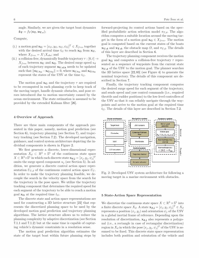
tory tracking (see Section 7.2). The developed navigation,

guidance, and control system architecture depicting the in-

dividual components is shown in Figure 2.

We first generate a discrete, lower-dimensional repre-

sentation Xd ⊂ R2 × S

1 of the continuous state space

X ⊂ R3×S

1 in which each discrete state xd,j = [xj , yj , ψj ]T

omits the surge speed component uj (see Section 5). In ad-

dition, we generate a discrete control action space repre-

sentation UU,d of the continuous control action space UU .

In order to make the trajectory planning feasible, we de-

couple the search in the velocity space from the search forthe trajectory in the pose space. We utilize the trajectory

tracking component that determines the required speed for

each segment of the trajectory to be able to reach a motion

goal xG at the required time tG.

The discrete state and action space representations are

used for constructing a 3D lattice structure [22] that rep-

resents the discretized planning space to be used by thedeveloped motion goal prediction and trajectory planning

algorithms. The lattice structure allows us to reduce the

planning complexity by adaptive discretization (see Section

7.1.1 and 7.1.2) but at the same time is capable of captur-

ing vehicle’s dynamic constraints in a resolution sense.

The motion goal prediction algorithm estimates the

state of the target boat within future planning steps by

forward-projecting its control actions based on the spec-

ified probabilistic action selection model πT,d. The algo-rithm computes a suitable location around the moving tar-

get in the form of a motion goal xG ∈ Xfree. The motion

goal is computed based on the current states of the boats

xU,d and xT,d, the obstacle map Ω, and πT,d. The detailsof this layer are described in Section 6.

The trajectory planning component receives the motion

goal xG and computes a collision-free trajectory τ repre-

sented as a sequence of waypoints from the current state

xU,d of the USV to the motion goal. The planner searchesthe 3D lattice space [22,83] (see Figure 4) to generate the

nominal trajectory. The details of this component are de-

scribed in Section 7.

Finally, the trajectory tracking component computes

the desired surge speed for each segment of the trajectory,and sends speed and yaw control commands (i.e., required

throttle and rudder positions) to the low-level controllers of

the USV so that it can reliably navigate through the way-

points and arrive to the motion goal at the required timetG. The details of this layer are described in Section 7.2.

Fig. 2: Developed USV system architecture for following a

moving target in a marine environment with obstacles.

5 State-Action Space Representation

We discretize the continuous state space X ⊂ R3 ×S

1 intoa finite discrete space Xd. A state xd,j = [xj , yj , ψj ]

T ∈ Xd

represents a position (xj , yj) and orientation ψj of the USV

in a global inertial frame of reference. Depending upon the

resolution of discretization, xd,j also represents a polygo-nal (i.e., a rectangle in case of rectangular discretization)

region inXd in which the pose [xj , yj , ψj ]T of the USV is as-

sumed to be fixed. This discrete state space representation

includes both position and orientation of the vehicle and

Target Following with Motion Prediction for Unmanned Surface Vehicle Operating in Cluttered Environments 7

hence is useful for incorporating constraints based on the

dynamics of the USV. Choosing a suitable discretizationof the lattice grid required trading off the speed and res-

olution completeness [58] of the planner. In our approach,

the discretization level was determined empirically by at-

tempting coarse discretization first and then increasing theresolution of the grid until it satisfied our task. The two

particular factors that we considered were the dimension

of the vehicle and its control action set.

Similarly, we discretize the continuous control action

space UU into a discrete control action set UU,d and mapeach control action uU,d,k ∈ UU,d to a reachable pose

[∆xk, ∆yk, ∆ψk]T in the body coordinate system of the

vehicle. Each control action is compliant with the vehicle’s

dynamics fU . We pre-compute the control actions in UU,dusing a hand-tuned PID controller. However, other control

techniques such as the sliding mode [79], backstepping [84],

etc. can be used [39]. An example of a discrete control ac-

tion set UU,d = uU,d,1, . . . ,uU,d,5 is shown in Figure 3a)

for the vehicle used in the experiments in Section 8. Thechoice of the number of control actions required trading off

the computational performance, resolution completeness of

the planner, and maneuverability of the vehicle. We have

determined the number of control actions empirically bystarting with three actions and then increasing their count

until it satisfied this trade-off. However, there have been

few techniques published recently that directly address the

design of control action sets [85,86,87,88,89] and as such

this problem is still an open research area.

We define a lattice L as a structure that maps xd,j to

xd,j,k using a control action uU,d,k for j = 1, 2, . . . , |S|

and k = 1, 2, . . . |UU,d|. The lattice thus represents an in-

stance of a graph with discrete states xd,j as nodes andactions uU,d,k as connecting arcs. Each action uU,d,k ∈

UU,d is used to establish a connection between dynamically

reachable nodes in L. For a node xd,j = [xj , yj , ψj ]T ∈

Xd, the neighbor corresponding to an action uU,d,k =

[∆xk, ∆yk, ∆ψk]T ∈ UU,d is given by Equation 1. The lat-

tice structure captures dynamics constraints in the form of

dynamically feasible connecting edges between the nodes

unlike orthogonal grids [58,22]. The lattice can also be ge-

ometrically viewed as multiple X-Y planning layers repre-senting 2D planning spaces with a fixed orientation ψ of

the USV as shown in Figure 4.

xd,j,k =

xjyjψj

+

cos∆ψj −sin∆ψj 0

sin∆ψj cos∆ψj 00 0 1

∆xk∆yk∆ψk

(1)

It is necessary to appropriately design the control ac-

tion set UU,d (i.e., the number, type, and duration of con-

trol actions) such that the required efficiency as well as the

quality of the nominal trajectory is achieved. In our ap-

proach, we manually designed the control action set usinga 3 degrees of freedom simulation model of the USV [83,23,

90]. To generate more complex actions, gradient-based op-

timization techniques [91] may be used. The control action

set can also be generated automatically using special tech-niques [85,86,87,88,89] that attempt to balance between

the computational efficiency and quality of the generated

trajectories.

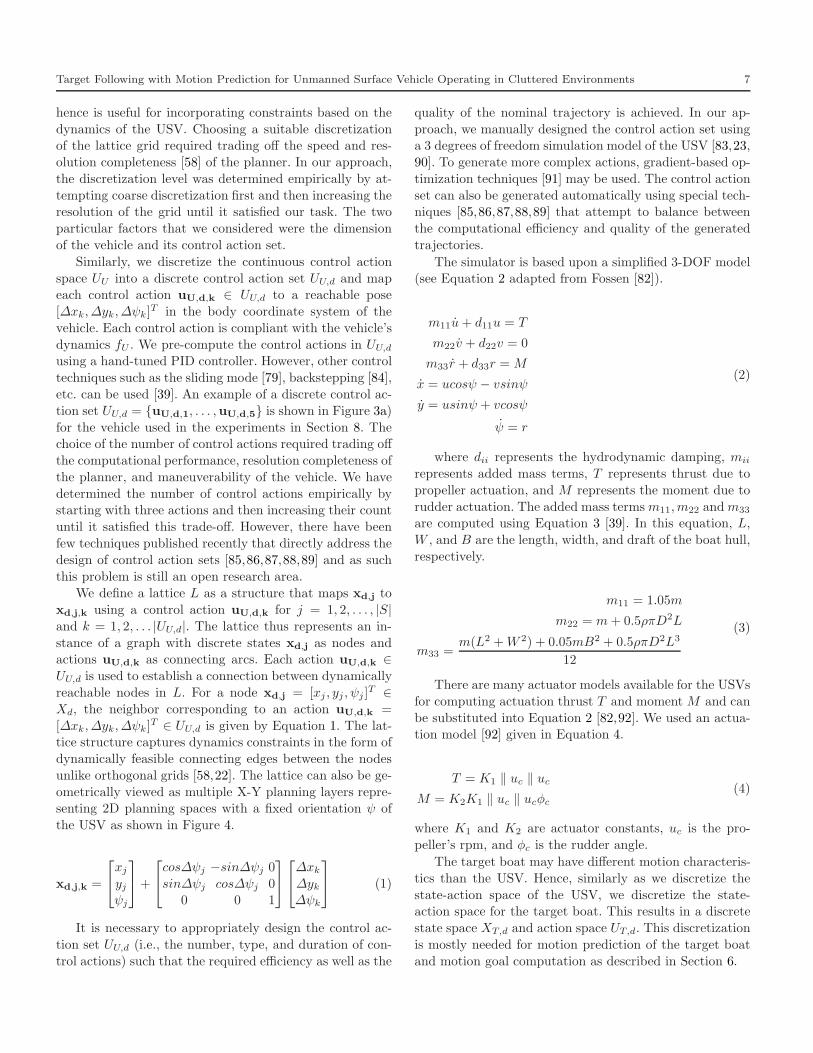
The simulator is based upon a simplified 3-DOF model(see Equation 2 adapted from Fossen [82]).

m11u+ d11u = T

m22v + d22v = 0

m33r + d33r =M

x = ucosψ − vsinψ

y = usinψ + vcosψ

ψ = r

(2)

where dii represents the hydrodynamic damping, mii

represents added mass terms, T represents thrust due to

propeller actuation, and M represents the moment due to

rudder actuation. The added mass termsm11,m22 andm33

are computed using Equation 3 [39]. In this equation, L,

W , and B are the length, width, and draft of the boat hull,

respectively.

m11 = 1.05m

m22 = m+ 0.5ρπD2L

m33 =m(L2 +W 2) + 0.05mB2 + 0.5ρπD2L3

12

(3)

There are many actuator models available for the USVs

for computing actuation thrust T and momentM and can

be substituted into Equation 2 [82,92]. We used an actua-tion model [92] given in Equation 4.

T = K1 ‖ uc ‖ uc

M = K2K1 ‖ uc ‖ ucφc(4)

where K1 and K2 are actuator constants, uc is the pro-

peller’s rpm, and φc is the rudder angle.

The target boat may have different motion characteris-

tics than the USV. Hence, similarly as we discretize the

state-action space of the USV, we discretize the state-action space for the target boat. This results in a discrete

state space XT,d and action space UT,d. This discretization

is mostly needed for motion prediction of the target boat

and motion goal computation as described in Section 6.

8 Petr Svec et al.

(a) A sparse control action set containing 5 actions. (b) A dense control action set containing 27 actions.

Fig. 3: Action sets for building the lattice data structure. The dense action set discretizes the action space into 27 control

actions. This set is particularly useful when a higher number of obstacles are present or demand on optimality is stricter.

However, the dense action set makes the planning speed slower due to more number of connected nodes in the planning

space, i.e., in the lattice.

Fig. 4: Planning space representation.

6 Motion Goal Prediction

To maintain a suitable distance between the USV and

the target boat, the motion goal predictor selects a desired

motion goal xG and arrival time tG. This is done by esti-mating the future poses of the target boat and then eval-

uating several candidate motion goals for the USV. Since

the motion goal must be computed relatively quickly, we

search for a sub-optimal solution by combining Monte-carlo

Algorithm 1 ComputeMotionGoal()

Input: The current poses xT,d and xU,d of the target boat andUSV, a probabilistic model of the target boat πT,d, and amap of obstacles Ω.

Output: A desired motion goal xG and arrival time tG.1: Let RT be a set of N randomly generated trajectories for

the target boat, where each trajectory τT,i ∈ RT begins atstate xT,d and time t0 and continues until time tk, suchthat each sampled action uT,d,j is selected with probabilityπT,d(xT,d,i,uT,d,j).

2: for each time point ti ∈ t1, t2, . . . tk do

3: for each trajectory τT,j ∈ RT do

4: Increment PT,i(xi,j , yi,j) by 1/N , where (xi,j , yi,j) isthe location of τT,j at time ti.

5: end for

6: Smooth PT,i by applying an m×m Gaussian kernel.7: Let (x∗i , y

∗

i ) be the location that maximizes PT,i(x∗i , y∗

i )and let ψ∗

i be the mean orientation at (x∗i , y∗

i ) across alltrajectories in RT at time ti.

8: Let xG,i ∈ XU,d = [xj , yj , uU , ψj ] be a candidate mo-tion goal for the USV which minimizes the distance to theprojected state, |(x∗i , y

∗

i )− (xj , yj)|+ α∆(ψ∗

i , ψj)9: end for

10: Let xG equal the candidate motion goal xG,i ∈ XG thatminimizes the cost function c(xG) and ensures a collision-free path up to time Tric

11: Compute a desired arrival time tG(xG) such that the USVwill arrive at xG shortly after the target boat

12: return (xG, tG(xG)).

sampling and heuristic evaluation techniques. The overall

process is described in Algorithm 1.

The action selection model πT,d : XT,d × UT,d → [0, 1]

defines a probability distribution over the target’s discretized

control actions at each pose xT,d ∈ XT,d. To explore thefuture poses of the target, we sample N random trajecto-

ries τT,j ∈ RT starting from the target’s current pose and

forward-projecting the target’s actions up to some finite

time horizon tk. During the sampling process, each control

Target Following with Motion Prediction for Unmanned Surface Vehicle Operating in Cluttered Environments 9

USVUSV

PT,3

PT,2

PT,1

Target boat

Sample

trajectories

Obstacles

(a)

USVUSV

xT,d,2

xT,d,3

xT,d,1

Candidate

trajectories

Candidate

motion goals

Target boat

(b)

Fig. 5: Motion goal prediction steps (a) Probability distri-

butions PT,1, PT,2 and PT,3, generated by sampling future

target trajectories at several time points. (b) Candidatemotion goals generated by selecting the most probable tar-

get pose.

action uT,d,k is selected with probability πT,d(xT,d,i,uT,d,k).

Sampled trajectories that lead to a collision with an obsta-cle are discarded from RT .

By recording the poses reached by the target boat along

each sampled trajectory, it is possible to estimate the prob-

ability PT,i(xj , yj) that the target will be at position (xj , yj)

at time ti. A two-dimensional Gaussian kernel is used tosmooth out the probability distribution represented by PT,i,

as illustrated in Figure 5. We also compute ψT,i(xj , yj), the

mean orientation at (xj , yj) across all samples at time ti.

For each time point ti ∈ t0, t1, . . . tk, the future posi-tion of the target boat can be approximated by

(x∗i , y∗

i ) = arg max(xj ,yj)

PT,i(xj , yj). (5)

Similarly, let ψ∗

i = ψT,i(x∗

i , y∗

i ) approximate of the future

orientation of the target boat. We select the candidate mo-tion goal xG,i ∈ XU,d = [xi, yi, uT , ψi]

T that is closest to

the projected target pose at time ti, such that

xG,i = arg minxG,j∈XU,d

|(x∗i , y∗

i )− (xj , yj)|+ α∆(ψ∗

i , ψj) (6)

where α∆(ψ∗

i , ψj) is the interior angle between ψ∗

i and ψjweighted by some parameter α.

Let g(xG,i) be the amount of time it takes the USV

to travel from its current location xU,d to the candidategoal xG,i. This can be computed by the A* heuristic search

process described in Section 7.

We define the cost function for motion goal xG,i as,

c(xG,i) =

δ−i(g(xG,i)− ti + 1), if g(xG,i) > tiδ−i, otherwise,

(7)

where g(xG,i) − ti is the estimated difference in arrival

time between the USV and target boat, and δ ∈ [0, 1] is

a discount factor. The smaller that δ is, the stronger the

bias towards earlier goals. From the set of candidate motiongoals XG, a final motion goal xG is selected such that the

cost function is minimized,

xG = arg minxG,i∈XG

c(xG,i). (8)

Given the final motion goal xG, the desired arrival time tGis determined by,

tG(xG) =

g(xG), if g(xG) > ti + tlagti + tlag, otherwise,

(9)

where tlag is the desired amount of time that the USV

should follow behind the target boat. This ensures that

the USV will reduce its speed when it can afford to do so,such as when it is already close the target boat.

Due to the cost function c(xG), the algorithm only con-

siders motion goals which guarantee a collision-free trajec-

tory for the USV up to some time Tric. States which leadto an inevitable collision are given an infinite cost, as de-

scribed in detail in Section 7.1. For simplicity, we may use

sampled poses from RT as motion goals if the dynamics

of the USV and target boat are equivalent, since the tra-

jectories in RT are guaranteed to be collision free. If nocollision-free motion goals are found, the algorithm will

default to the currently assigned motion goal.

7 Trajectory Planning and Tracking

7.1 Nominal Trajectory Planning

The nominal trajectory planner generates a collision free

trajectory τ : [0, t] → Xfree between the current state xU

of the USV and the motion goal xG in the obstacle field

Ω. The trajectory τ is computed by concatenating controlactions in UU,d which are designed a-priori. The planner is

based on A* heuristic search [21] over the lattice. The plan-

ner associates xG and xU with their closest corresponding

states xG,d and xU,d in the lattice L. Similarly, the plan-ner maps the state of every obstacle xO ∈ X to its closest

corresponding state xO,d ∈ Xd.

We also extract the region of inevitable collision [25] in

Xd for the given obstacle field Ω. In general, the region of

inevitable collision is defined as a set of states that lead to acollision regardless of a control action the vehicle executes.

We avoid searching for the trajectory in this region (i.e.,

during the search, we do not expand candidate states that

fall into this region) by assigning an infinite cost to all itsstates.

In this paper, we approximate the region of inevitable

collision by determining a set of lattice nodes from which

the vehicle will collide with an obstacle after a specified

10 Petr Svec et al.

time horizon. In the computation, we assume that the ve-

hicle will continue in its course by moving straight andwith maximum speed. This is generally a valid assumption

as the length scale of the control action is much smaller

and possibility of sudden steering is less in such a small

distance. In addition, our 3D pose based representationtakes orientation of the USV into account. A USV that is

very close to an obstacle can be said to be inside the re-

gion of inevitable collision if it is approaching the obstacle.

On the other hand, if the USV is moving away from the

obstacle from the same pose then it can be said to be outof the region of inevitable collision.

More formally, for each lattice node xd,j ∈ Xd that

represents a pose [xj , yj , ψj ]T of the USV, we use the dy-

namic model of the vehicle to determine a lattice node x′

d,j

that represents the vehicle’s pose after the time Tric. If the

forward projected lattice node x′

d,j lies on an obstacle, i.e.,

Ω(x′

d,j) = 1, then we label xd,j to be lying inside the region

of inevitable collision (see Equation 10).

RIC(xd,j, umax, Tric) =

1, if x′

d,j ∈ Ω

0, otherwise,(10)

In Equation 10, x′

d,j is the lattice node closest to the

actual state x′

j = xj + Tricumax[cosψj , sinψj , 0, 0]T , and

umax is the maximum surge speed of the vehicle.

The time horizon Tric for determining the region of in-

evitable collision can be set by the user of the planning

algorithm depending upon the preferred allowable risk. Inparticular, in this paper, we set Tric experimentally based

on a state transition model of the USV (i.e., a probabilis-

tic state transition function) which was developed in our

previous work [83]. The state transition model gives us a

probability distribution over future states of the vehiclegiven its initial state, a control action set, and sea state.

We developed this model using Monte Carlo runs of a high-

fidelity 6 DOF dynamics simulation of interaction between

the USV and ocean waves. Our simulator can handle anyUSV geometry, dynamics parameters, and sea state. This

approach for computing the region of inevitable collision

allows us to more precisely define the size of the collision

zones and thus make the planner less conservative when

planning in narrow regions.

During the search for the trajectory, lattice nodes are

incrementally expanded towards xG,d in the least-cost fash-

ion according to the trajectory cost f(xd) = g(xd)+h(xd),

where g(xd) is the optimal cost-to-come from xU,d to xd,and h(xd) is the heuristic cost-to-go between xd and xG,d.

The admissible heuristic cost function h(xd) (i.e., not al-

lowed to overestimate the actual cost of the trajectory)

reduces the total number of expanded nodes in the lat-

tice as per the A* graph search algorithm that guarantees

optimality of the computed plan.

The cost function was designed in terms of trajectory

length. The cost-to-come g(xd) represents the total length

of a trajectory between the current state xU,d of the vehicle

and xd and is computed as g(xd) =∑K

k=1 l(uU,d,k) over

K planning stages, where l(uU,d,k) is the length of the pro-

jected control action uU,d,k ∈ UU,d. If the control action

uU,d takes the vehicle to a collision state xcol,d (i.e., the

state for which Ω(xcol,d) = 1 or RIC(xcol,d, umax, Tric) =1), then l(uU,d) is set to ∞. Each control action is sam-

pled using intermediate waypoints. These waypoints are

then used for collision checking. The heuristic cost h(xd)

is represented as the Euclidean distance between xd andxG,d. Alternatively, according to [22], one can utilize a pre-

computed look-up table containing heuristic costs of tra-

jectories between different pairs of states in an environment

without obstacles.

The dynamically feasible trajectory τ is a sequenceuU,d,1,uU,d,2, . . . ,uU,d,K of precomputed atomic con-

trol actions, where uU,d,k ∈ UU,d for k = 1, . . . ,K. This

sequence of control actions is then translated into a se-

quence of K + 1 waypoints wd,1, . . . ,wd,K+1 leading tothe motion goal xG,d. Thus, the generated nominal trajec-

tory is guaranteed to be dynamically feasible and ensures

that the USV will be able to progressively reach the way-

points in a sequence without substantial deviations, which

otherwise may lead to collisions.

In case of the described follow task, the motion goal

keeps changing dynamically and hence the trajectory plan-

ner needs to compute the plans repeatedly. For this reason,

the planner must be very fast and efficient. For the very re-

quirement of following the target boat in a cluttered space,the planning space must be 3D pose based. A higher di-

mensional planning space may significantly slow down the

trajectory planner. For this reason, we enhanced the com-

putational performance of the planner by (a) superimpos-ing higher and reduced dimension state spaces, and (b)

utilizing a control action set with multiple levels of reso-

lution. These two extensions are explained in detail in the

following two subsections.

7.1.1 Superimposition of Higher and Reduced Dimension

State Spaces

Superimposing pose based 3D lattice and position based

2D grid state space representations can improve planner

performance by sacrificing allowable level of optimality. Atcloser distances (i.e., g(xd) < β) from the initial state

xU,d, the planning space is chosen to be a 3D lattice,

whereas at a farther distance (i.e., g(xd) ≥ β) the plan-

ning space is chosen to be a 2D grid. This scheme is useful

Target Following with Motion Prediction for Unmanned Surface Vehicle Operating in Cluttered Environments 11

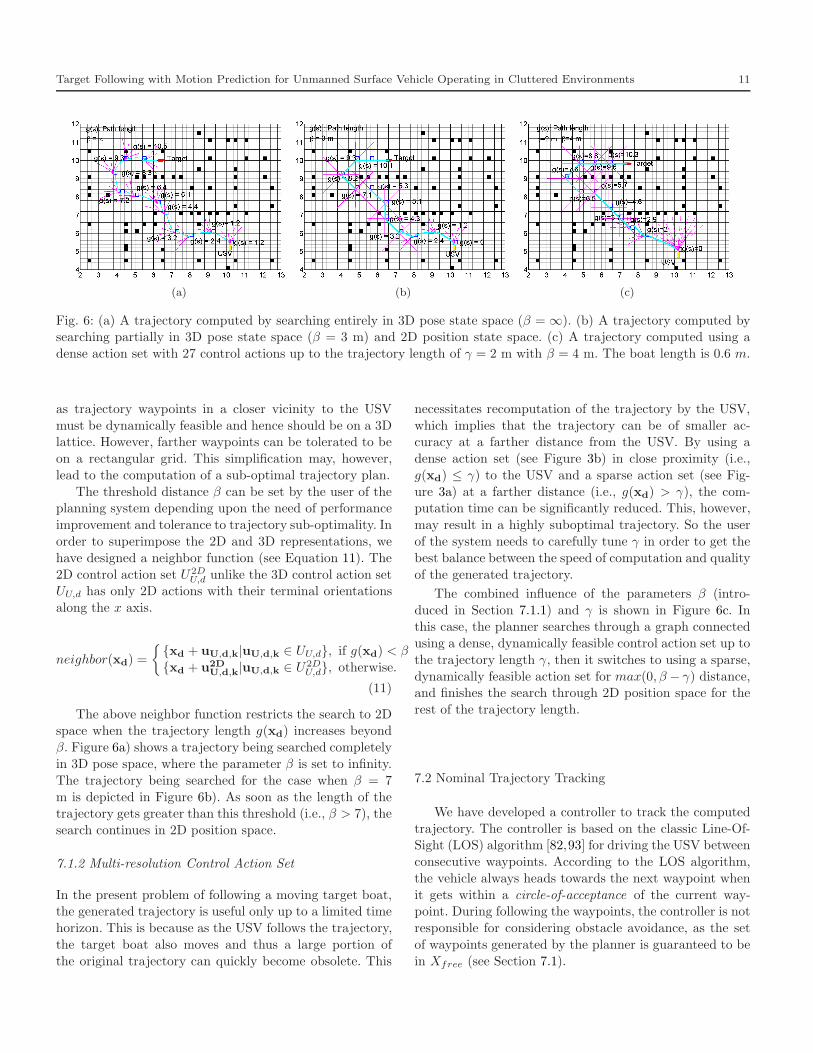
(a) (b) (c)

Fig. 6: (a) A trajectory computed by searching entirely in 3D pose state space (β = ∞). (b) A trajectory computed bysearching partially in 3D pose state space (β = 3 m) and 2D position state space. (c) A trajectory computed using a

dense action set with 27 control actions up to the trajectory length of γ = 2 m with β = 4 m. The boat length is 0.6 m.

as trajectory waypoints in a closer vicinity to the USV

must be dynamically feasible and hence should be on a 3Dlattice. However, farther waypoints can be tolerated to be

on a rectangular grid. This simplification may, however,

lead to the computation of a sub-optimal trajectory plan.

The threshold distance β can be set by the user of theplanning system depending upon the need of performance

improvement and tolerance to trajectory sub-optimality. In

order to superimpose the 2D and 3D representations, we

have designed a neighbor function (see Equation 11). The

2D control action set U2DU,d unlike the 3D control action set

UU,d has only 2D actions with their terminal orientations

along the x axis.

neighbor(xd) =

xd + uU,d,k|uU,d,k ∈ UU,d, if g(xd) < β

xd + u2DU,d,k|uU,d,k ∈ U2D

U,d, otherwise.

(11)

The above neighbor function restricts the search to 2Dspace when the trajectory length g(xd) increases beyond

β. Figure 6a) shows a trajectory being searched completely

in 3D pose space, where the parameter β is set to infinity.

The trajectory being searched for the case when β = 7

m is depicted in Figure 6b). As soon as the length of thetrajectory gets greater than this threshold (i.e., β > 7), the

search continues in 2D position space.

7.1.2 Multi-resolution Control Action Set

In the present problem of following a moving target boat,the generated trajectory is useful only up to a limited time

horizon. This is because as the USV follows the trajectory,

the target boat also moves and thus a large portion of

the original trajectory can quickly become obsolete. This

necessitates recomputation of the trajectory by the USV,

which implies that the trajectory can be of smaller ac-curacy at a farther distance from the USV. By using a

dense action set (see Figure 3b) in close proximity (i.e.,

g(xd) ≤ γ) to the USV and a sparse action set (see Fig-

ure 3a) at a farther distance (i.e., g(xd) > γ), the com-putation time can be significantly reduced. This, however,

may result in a highly suboptimal trajectory. So the user

of the system needs to carefully tune γ in order to get the

best balance between the speed of computation and quality

of the generated trajectory.

The combined influence of the parameters β (intro-

duced in Section 7.1.1) and γ is shown in Figure 6c. Inthis case, the planner searches through a graph connected

using a dense, dynamically feasible control action set up to

the trajectory length γ, then it switches to using a sparse,

dynamically feasible action set for max(0, β − γ) distance,and finishes the search through 2D position space for the

rest of the trajectory length.

7.2 Nominal Trajectory Tracking

We have developed a controller to track the computed

trajectory. The controller is based on the classic Line-Of-Sight (LOS) algorithm [82,93] for driving the USV between

consecutive waypoints. According to the LOS algorithm,

the vehicle always heads towards the next waypoint when

it gets within a circle-of-acceptance of the current way-point. During following the waypoints, the controller is not

responsible for considering obstacle avoidance, as the set

of waypoints generated by the planner is guaranteed to be

in Xfree (see Section 7.1).

12 Petr Svec et al.

Algorithm 2 ComputeDesiredSpeed(): Compute de-

sired surge speed for all segments of the trajectory τ so

that the USV can reach its motion goal xG at the required

time tG.

Input: A trajectory τ = uU,d,kKk=1that defines the max-

imum allowable speed ud,k,max for each of its segmentsuU,d,k, and the required arrival time tG to the motion goalxG.

Output: Desired surge speeds Vd = ud,kKk=1for all trajectory

segments uU,d,kKk=1.

1: Compute initial desired surge speeds Vd = ud,kKk=1for all

segments of the trajectory τ . The initial speed is computed asud,k = L/tG, where L =

∑Kk=1

l(uU,d,k) is the total lengthof the trajectory and l(uU,d,k) is the length of the trajectorysegment uU,d,k.

2: Let Q be the priority queue containing the trajectory seg-ments uU,d,kKk=1

in ascending order according to theirmaximum allowable surge speed ud,k,max.

3: while Q not empty do

4: Remove a segment uU,d,k ← Q.First() from Q with theminimum allowable surge speed ud,k,max.

5: Compute the time lost tlost = td,k,max − td,k whentraversing uU,d,k with ud,k,max. The time needed to tra-verse the segment uU,d,k under the constraint ud,k,max

is td,k,max = l(uU,d,k)/ud,k,max, whereas td,k =l(uU,d,k)/ud,k is the time it takes to traverse the segmentwith the desired speed.

6: if tlost > 0 then

7: Set ud,k ← ud,k,max in Vd.8: Set ud,l = l(uU,d,l)/(td,l − tlost/|Q|) for all remaining

segments l 6= k, where td,l = l(uU,d,l)/ud,l.9: end if

10: end while

11: return Vd.

The boat dynamics considered in this paper is under-

actuated and hence its speed in the sway direction cannot

be controlled directly. The control required to follow way-

points must be divided between surge speed and headingcontrollers. We accomplish this by using a PID based cas-

caded surge speed u and yaw ψ rate controllers. The head-

ing controller produces corresponding rudder commands.

We assume that the roll and pitch is maintained to zero.

The desired heading angle at ith time instance is calcu-

lated using ψU,d = atan2(yi−y, xi−x), where [x, y]T is the

current position of the USV and wd,i = [xi, yi, ui]T is the

current active waypoint, where ui is the desired speed for

reaching this waypoint. After this, the yaw error is com-

puted using eψU= ψU,d − ψU , where ψU is the current

orientation of the USV. The yaw error is then used by the

PID controller to obtain the control action, i.e., the rudderangle φi.

φi = PyaweψU+ Iyaw

∫

eψUdt+Dyaw

deψU

dt(12)

In Equation 12, Pyaw, Iyaw, and Dyaw are proportional,

integral, and derivative parameters of the PID controller,respectively.

Due to the discretization of the state and control action

spaces, there may occur small gaps between two consecu-

tive control actions in the computed trajectory (see Fig.

6a). In order to ensure reliable tracking of such trajectory,we define a region of acceptance around each waypoint and

increase the size of the collision zones around the obstacles

to minimize the probability of a collision. This also resolves

other possible tracking problems that may arise because ofthe approximation of USV’s dynamics when computing the

control action set for the trajectory planner. Moreover, this

also prevents creation of loops when the vehicle is not able

to precisely reach a given waypoint. It is possible to design

control actions such that they connect seamlessly. However,this requires substantial design effort. Lastly, since the tra-

jectory is recomputed with a high frequency and the con-

troller always follows the first few, dynamically-reachable

waypoints along the trajectory, the USV will not experi-ence the discontinuous transition between 3D and 2D lat-

tices (see Section 7.1).

In the follow task, the controller must be able to handle

variations in the surge speed during steep turns. Each seg-

ment uU,d,k of the trajectory τ thus defines the maximumallowable surge speed ud,k,max of the vehicle. In addition,

the USV cannot immediately decrease its surge speed be-

fore turning, rather it should start decelerating in advance

to attain the desired speed near the turn.

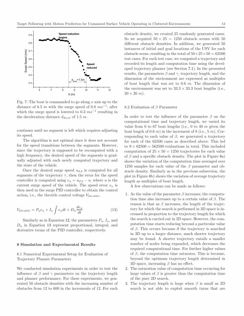
In our experiments, we selected a higher speed of 0.8ms−1 for straight segments of the trajectory while a smaller

speed of 0.3 ms−1 for turns. We determine the distance

ddecel required for the USV to decelerate to a given surge

speed using physical experiments. Figure 7 shows the re-sult of an experimental test to determine ddecel. In this

test, we controlled the boat to go in a straight line along

the x axis with a surge speed of 0.8 ms−1. At a distance of

8.5 m, the boat was commanded to reduce its surge speed

to 0.3 ms−1. We used PID controller for controlling thesurge speed. We determined that the boat needs to run for

about ddecel = 1.5 m in order to decelerate to the desired

speed of 0.3 ms−1.

We adjust the desired surge speed ud,k of each trajec-

tory segment uU,d,k (i.e., the desired speed for reachingeach waypoint wd,k) so that the USV arrives to xG at

the required time tG. We compute the desired speed it-

eratively (see Algorithm 2) given the maximum allowable

surge speed ud,k,max constraint defined for each segment ofthe trajectory. We start with the segment with the mini-

mum allowable speed, compute the time lost while travers-

ing this segment, and uniformly increase the speed of other

segments to compensate for the time loss. The algorithm

Target Following with Motion Prediction for Unmanned Surface Vehicle Operating in Cluttered Environments 13

6 7 8 9 10 11 12

0.3

0.4

0.5

0.6

0.7

0.8

0.9

Speed reduced

Sur

ge S

peed

(m/s

)

X (m)

Speed reduction begins

ddecel

=1.5m

Fig. 7: The boat is commanded to go along x axis up to the

distance of 8.5 m with the surge speed of 0.8 ms−1, after

which the surge speed is lowered to 0.3 ms−1 resulting in

the deceleration distance ddecel of 1.5 m.

continues until no segment is left which requires adjustingits speed.

The algorithm is not optimal since it does not account

for the speed transitions between the segments. However,

since the trajectory is supposed to be recomputed with a

high frequency, the desired speed of the segments is grad-

ually adjusted with each newly computed trajectory andthe state of the vehicle.

Once the desired surge speed ud,k is computed for all

segments of the trajectory τ , then the error for the speed

controller is computed using eu = ud,k − u, where u is the

current surge speed of the vehicle. The speed error eu isthen used in the surge PID controller to obtain the control

action, i.e., the throttle control voltage Vthrottle.

Vthrottle = Pueu + Iu

∫

eudt+Du

deudt

(13)

Similarly as in Equation 12, the parameters Pu, Iu, andDu in Equation 13 represent proportional, integral, and

derivative terms of the PID controller, respectively.

8 Simulation and Experimental Results

8.1 Numerical Experimental Setup for Evaluation ofTrajectory Planner Parameters

We conducted simulation experiments in order to test theinfluence of β and γ parameters on the trajectory length

and planner performance. For these experiments, we gen-

erated 50 obstacle densities with the increasing number of

obstacles from 12 to 600 in the increments of 12. For each

obstacle density, we created 25 randomly generated cases.

So we acquired 50 × 25 = 1250 obstacle scenes with 50different obstacle densities. In addition, we generated 50

instances of initial and goal locations of the USV for each

obstacle scene, resulting in the total of 50×25×50 = 62500

test cases. For each test case, we computed a trajectory andrecorded its length and computation time using the devel-

oped trajectory planner (see Section 7.1). In the presented

results, the parameters β and γ, trajectory length, and the

dimension of the environment are expressed as multiples

of boat length that was set to 0.6 m. The dimension ofthe environment was set to 33.3 × 33.3 boat lengths (i.e.,

20× 20 m).

8.2 Evaluation of β Parameter

In order to test the influence of the parameter β on the

computational time and trajectory length, we varied itsvalue from 0 to 67 boat lengths (i.e., 0 to 40 m given the

boat length of 0.6 m) in the increment of 8 (i.e., 5 m). Cor-

responding to each value of β, we generated a trajectory

for each of the 62500 cases as described above. This ledto 9 × 62500 = 562500 evaluations in total. This included

computation of 25× 50 = 1250 trajectories for each value

of β and a specific obstacle density. The plot in Figure 8a)

shows the variation of the computation time averaged over

1250 samples for each value of the β parameter and ob-stacle density. Similarly as in the previous subsection, the

plot in Figure 8b) shows the variation of average trajectory

length as multiples of boat length.

A few observations can be made as follows:

1. As the value of the parameter β increases, the computa-

tion time also increases up to a certain value of β. The

reason is that as β increases, the length of the trajec-tory for which the search is performed in 3D space is in-

creased in proportion to the trajectory length for which

the search is carried out in 2D space. However, the com-

putation time starts reducing beyond a particular valueof β. This occurs because if the trajectory is searched

in 3D up to a larger distance, much shorter trajectory

may be found. A shorter trajectory entails a smaller

number of nodes being expanded, which decreases the

required computational time. For further higher valuesof β, the computation time saturates. This is because,

beyond the optimum trajectory length determined in

3D space, increasing β has no effect.

2. The saturation value of computation time occurring forlarge values of β is greater than the computation time

of the pure 2D search.

3. The trajectory length is large when β is small as 2D

search is not able to exploit smooth turns that are

14 Petr Svec et al.

020

4060

0

5000

10000

15000

20000

25000

100200300400500600

Ave

rage

com

puta

tion

time

(ms)

Numbe

r of o

bstac

les

boat length)

020

4060

30

32

34

36

38

40

42

44

46

2030

405060

Ave

rage

traj

ecto

ry le

ngth

( b

oat l

engt

h)

Numbe

r of o

bstac

les

( boat length)

(a) (b)

Fig. 8: Variation of the average trajectory computation time (see plot a)) and trajectory length (see plot b)) with respect

to the trajectory length threshold β for switching between 3D and 2D representations of the state space.

020

4060

0

5000

10000

15000

20000

25000

30000

35000

100200300400500600

Ave

rage

com

puta

tion

time

(ms)

Numbe

r of o

bstac

les

( boat length)

020

4060

28

30

32

34

36

38

40

42

44

100200300400500600

Ave

rage

traj

ecto

ry le

ngth

( b

oat l

engt

h)

Numbe

r of o

bstac

les

( boat length)

(a) (b)

Fig. 9: Variation of the average trajectory computation time (see plot a)) and trajectory length (see plot b)) with respect

to the trajectory length threshold γ for switching between a control action set consisting of 27 and 5 control actions.

possible using 3D lattice based search. This however

is not true in general for all cases. For example, a lat-tice based structure will prevent transitions to adjoin-

ing states due to inbuilt vehicle constraints. However,

we would like to report here that in general, the aver-

age case trajectory length can be smaller for a latticesearch as compared to pure 2D search.

4. The value of β should be chosen such that it does not lie

in the peaked region. From the experimental test cases

we can determine the prohibited regions of β in which

computation performance becomes worse for a given

obstacle density. In other words, there is a certain range

of β for a given obstacle density for which the plannerperformance gets deteriorated, however, any value of β

less than that will result in performance improvement.

This improvement in the performance, however, will

have an adverse effect on the optimality of the gener-ated trajectories. This can be observed from the plot of

trajectory length variation versus the parameter β (see

Figure 8b)), which shows that for smaller β, the lengths

of trajectories are greater. A balance can be chosen by

the user of the algorithm to get performance gain by

Target Following with Motion Prediction for Unmanned Surface Vehicle Operating in Cluttered Environments 15

020

4060

0

500

1000

1500

2000

0

20

4060

Ave

rage

com

puta

tion

time

(ms)

( boat

length

)

( boat length)

020

4060

26

28

30

32

34

0

20

40

60

Ave

rage

traj

ecto

ry le

ngth

( b

oat l

engt

h)

( boat

length

)

( boat length)

(a) (b)

020

4060

0

200

400

600

800

1000

1200

1400

1600

0

20

4060

Ave

rage

com

puta

tion

time

(ms)

boat

length

)

( boat length)

020

4060

26

28

30

32

34

36

38

40

0

20

40

60

Ave

rage

traj

ecto

ry le

ngth

( b

oat l

engt

h)

( boat

length

)

( boat length)

(c) (d)

Fig. 10: Variation of the average computation time with threshold parameters γ and β for 120 (see plot a)) and 300

obstacles (see plot c)) in the scene. Variation of the average trajectory length with threshold parameters γ and beta for120 (see plot b)) and 300 obstacles (see plot d)) in the scene.

incurring allowable loss of optimality of the computedtrajectory.

8.3 Evaluation of γ Parameter

In order to test the influence of the parameter γ on the

computational time and trajectory length, we varied its

value from 0 to 67 boat lengths in the increment of 8 as de-

scribed above for the parameter β. This lead to 9×62500 =562500 evaluations in total. For each γ and obstacle scene

we generated 1250 trajectories. The plot in Figure 9a)

shows the variation of the computation time averaged over

1250 samples for each value of the γ parameter and ob-

stacle density. Similarly, the plot in Figure 9b) shows thevariation of average trajectory length.

A few observations can be made as follows:

1. As the parameter γ increases, the average computa-

tion time also increases. This is because the trajectory

is searched in a densely connected lattice up to γ dis-tance of trajectory length, after which the sparsely con-

nected lattice is used. However, beyond a certain limit

of γ, the trajectory length gets smaller, causing lesser

number of nodes being expanded and hence, the com-putation time reduces again. This effect is similar to the

effect observed with the parameter β. The computation

time saturates at values greater than optimal trajectory

length searched in the densely connected lattice.

16 Petr Svec et al.

2. The saturation value of the computational time occur-

ring for large values of γ (searched purely in denselyconnected lattice) is higher than that of very small val-

ues of γ (searched purely in sparsely connected lattice).

3. The average trajectory length reduces as γ increases

because trajectory searched in a dense lattice (i.e., dueto a large value of γ) is more optimal compared to the

one searched in a sparsely connected lattice.

4. The value of γ should be chosen such that it does not lie

in the peaked region. From the experimental test cases,

we can determine the prohibited regions of γ in whichcomputation performance becomes worse for a given

obstacle density. This is again similar to the behavior

of β parameter.

8.4 Evaluation of Combined Effect of β and γ Parameters

In order to study the combined influence of β and γ pa-

rameters, we have designed a test case, with β and γ vary-

ing from 0 to 67 of boat lengths. It should be noted thatβ ≥ γ, as the influence of γ (i.e., computing in densely

connected lattice) takes priority over the influence of β.

For each combination of the parameters γ and β we ran

tests in two obstacle densities (namely with 120 and 300

obstacles). For each obstacle density we ran 25 randomlygenerated cases as described before. This resulted in run-

ning 62500 cases and computing a trajectory for each case.

The variation of average trajectory lengths and computa-

tion time is illustrated in Figures 10a-d). The plots showthe prohibited regions for each combination of β and γ. In

these regions, average computation time increases.

8.5 Simulation Results of Overall Planning Approach

To evaluate the motion goal prediction algorithm described

in Section 6 we conducted a series of simulation experi-

ments using randomly generated test cases. Each test case

consisted of a fixed trajectory for the target boat and a setof 48, 72, 96, 120 or 144 randomly placed obstacles in an

environment with the dimension of 33 × 33 boat lengths

(i.e., 20 × 20 m). We generated 200 different trajectories

for a total of 1000 different test cases. An example test case

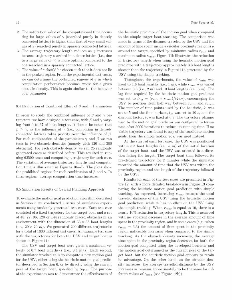
with the trajectories for both the USV and target boat isshown in Figure 11c.

The USV and target boat were given a maximum ve-

locity of 0.7 boat lengths/s (i.e., 0.4 m/s). Each second,

the simulator invoked calls to compute a new motion goalfor the USV, either using the heuristic motion goal predic-

tor described in Section 6, or by directly using the current

pose of the target boat, specified by xT,d. The purpose

of the experiments was to demonstrate the effectiveness of

the heuristic predictor of the motion goal when compared

to the simple target boat tracking. The comparison wasmade in terms of the distance traveled by the USV and the

amount of time spent inside a circular proximity regionXP

around the target, specified by minimum radius rmin and

maximum radius rmax. Figure 11b illustrates the reductionin trajectory length when using the heuristic motion goal

predictor with a trajectory approximately 3.3 boat lengths

shorter than the trajectory in Figure 11a generated by the

USV using the simple tracking.

Throughout the experiments, the value of rmin wasfixed to 1.6 boat lengths (i.e., 1 m), while rmax was varied

between 3.3 (i.e., 2 m) and 10 boat lengths (i.e., 6 m). The

lag time required by the heuristic motion goal predictor

was set to tlag = (rmin + rmax)/(2uU ), encouraging the

USV to position itself half way between rmin and rmax.The number of time points used by the heuristic, k, was

set to 5 and the time horizon, tk, was set to 10 s, and the

discount factor, δ, was fixed at 0.9. The trajectory planner

used by the motion goal predictor was configured to termi-nate after 5000 iterations to reduce its running time. If no

viable trajectory was found to any of the candidate motion

goals, then the simple motion goal was used instead.

At the start of each test case, the USV was positioned

within 8.3 boat lengths (i.e., 5 m) of the initial locationof the target boat, and the USV was oriented in a direc-

tion facing the target. The target boat then followed its

pre-defined trajectory for 2 minutes while the simulator

recorded the amount of time that the USV was within the

proximity region and the length of the trajectory followedby the USV.

Results for each of the test cases are presented in Fig-

ure 12, with a more detailed breakdown in Figure 13 com-

paring the heuristic motion goal prediction with simple

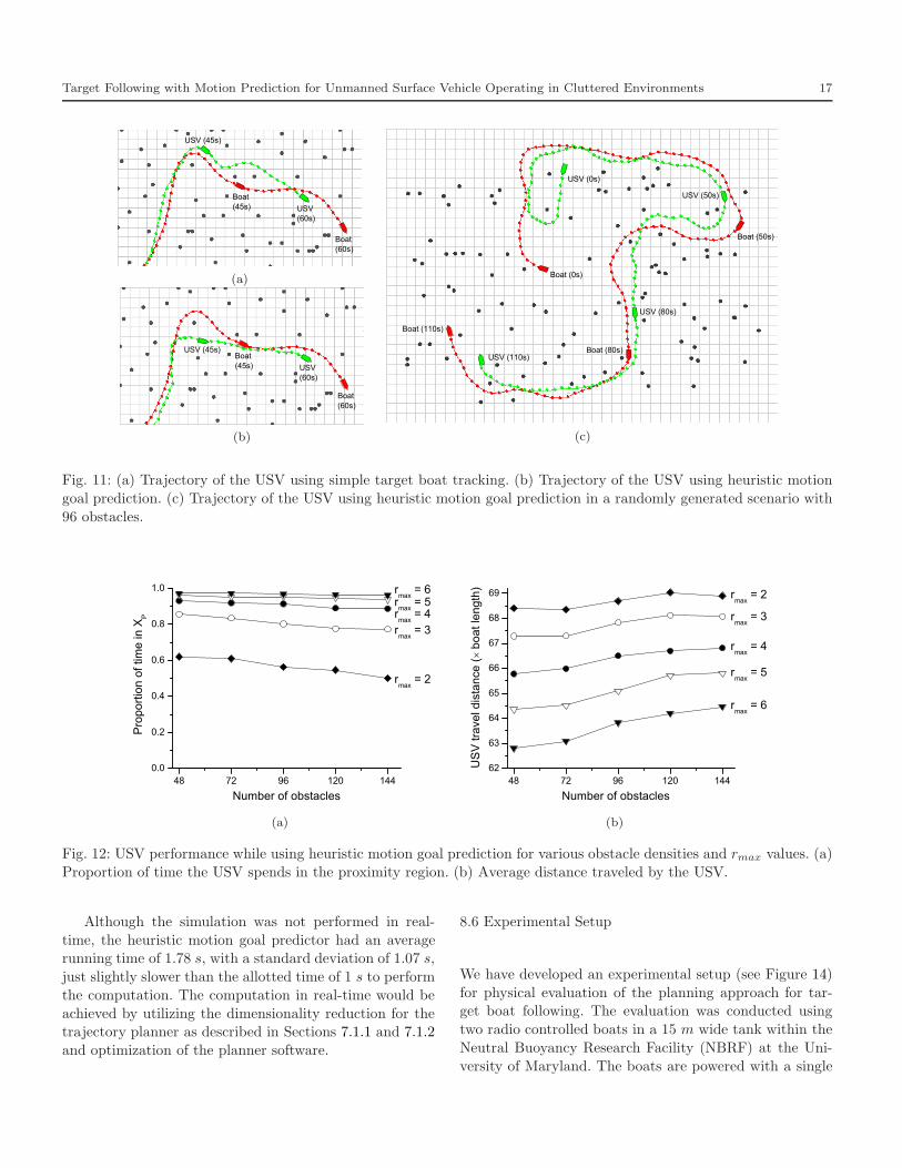
tracking. As expected, increasing rmax reduces the totaltraveled distance of the USV using the heuristic motion

goal prediction, while it has no effect on the USV using

the simple tracking. When rmax is equal to 10, there is a

nearly 10% reduction in trajectory length. This is achievedwith no apparent decrease in the average amount of time

spent in the proximity region, and in some cases (e.g., when

rmax = 3.3) the amount of time spent in the proximity

region noticeably increases when compared to the simple

tracking. As the obstacle density increases, the averagetime spent in the proximity region decreases for both the

motion goal computed using the developed heuristic and

the motion goal determined as the current pose of the tar-

get boat, but the heuristic motion goal appears to retainits advantage. On the other hand, as the obstacle den-

sity increases, the average travelled distance by the USV

increases or remains approximately to be the same for dif-

ferent values of rmax (see Figure 12b)).

Target Following with Motion Prediction for Unmanned Surface Vehicle Operating in Cluttered Environments 17

USV

(60s)

Boat

(60s)

USV (45s)

Boat

(45s)

(a)

USV (0s)

Boat (0s)

Boat (50s)

USV (50s)

USV (80s)

Boat (80s)

Boat (110s)

USV (110s)

(c)

USV (45s)

USV

(60s)

Boat

(60s)

Boat

(45s)

(b)

Fig. 11: (a) Trajectory of the USV using simple target boat tracking. (b) Trajectory of the USV using heuristic motion

goal prediction. (c) Trajectory of the USV using heuristic motion goal prediction in a randomly generated scenario with

96 obstacles.

48 72 96 120 1440.0

0.2

0.4

0.6

0.8

1.0

Pro

porti

on o

f tim

e in

XP

Number of obstacles

rmax

= 6r

max = 5

rmax

= 4r

max = 3

rmax

= 2

(a)

48 72 96 120 14462

63

64

65

66

67

68

69

rmax

= 6

rmax

= 5

rmax

= 4

rmax

= 3

US

V tr

avel

dis

tanc

e (

boa

t len

gth)

Number of obstacles

rmax

= 2

(b)

Fig. 12: USV performance while using heuristic motion goal prediction for various obstacle densities and rmax values. (a)

Proportion of time the USV spends in the proximity region. (b) Average distance traveled by the USV.

Although the simulation was not performed in real-

time, the heuristic motion goal predictor had an averagerunning time of 1.78 s, with a standard deviation of 1.07 s,

just slightly slower than the allotted time of 1 s to perform

the computation. The computation in real-time would be

achieved by utilizing the dimensionality reduction for thetrajectory planner as described in Sections 7.1.1 and 7.1.2

and optimization of the planner software.

8.6 Experimental Setup

We have developed an experimental setup (see Figure 14)

for physical evaluation of the planning approach for tar-get boat following. The evaluation was conducted using

two radio controlled boats in a 15 m wide tank within the

Neutral Buoyancy Research Facility (NBRF) at the Uni-

versity of Maryland. The boats are powered with a single

18 Petr Svec et al.

0.0

0.2

0.4

0.6

0.8

1.0

Simple tracking Heuristic prediction

rmax

( boat length)

Pro

porti

on o

f tim

e in

XP

108.36.653.3

(a)

57

60

63

66

69

72

75

Simple tracking Heuristic prediction

US

V tr

avel

dis

tanc

e (

boa

t len

gth)

108.36.65r

max ( boat length)

3.3

(b)

Fig. 13: Comparison of simple and heuristic motion goal prediction for a set of 200 randomly generated test cases with96 obstacles.(a) Portion of time the USV spends in the proximity region. (b) Average distance traveled by the USV. For

each figure, the box plot shows the median, upper and lower quartile. The whiskers show the upper and lower decile. The

mean value is represented by a small square.

Fig. 14: Developed physical setup for testing autonomous behaviors in the Neutral Buoyancy Research Facility (NBRF)

at the University of Maryland. The developed planner for following the target boat is represented as a follow behaviorexecuted by the behavior selection and execution components of the entire system.

Target Following with Motion Prediction for Unmanned Surface Vehicle Operating in Cluttered Environments 19

(a) (b) (c)

(d) (e) (f)

Fig. 15: Experimental result of the developed planning approach for following a target boat by an autonomous surface

vehicle (USV) in an environment with static obstacles. The case f) illustrates a situation in which the USV takes ashortcut while following the target boat.

9.6 volt battery and consist of one DC motor to controlthe forward and reverse speed of the propeller and a servo

motor to control the angular motion of rudder. We use

Hitec transmitter and receiver pair which operates on 2.4

GHz bandwidth. We utilize Endurance PCTx interface be-

tween the laptop and the RC transmitter to allow radiotransmission of actuator commands to control the throttle

and rudder positions of the autonomous USV. The USV

is remotely controlled by the developed nominal trajectory

planner and trajectory tracking controller running on alaptop. The setup also allows us to control the target boat

using a remote controller interface.

The positions of the boats are perceived using a vision

system that includes a single fish eye lens camera mounted

8 m above the level of the pool. We have developed a color

blob detection image processing algorithm to detect theboats. The USV as well as the target boat use SMD LEDs

with high intensity to be easily recognizable by the blob

detection algorithm.

We have also developed a camera calibration module to

relate the measured entire pool area to a local coordinate

frame of the USV planning system running on a laptop.The calibration of the camera provides us a model of its

geometry as well as distortion model of the lens. The cal-

ibration system uses three reference lines with the same

color markers separated by a fixed distance of 1.5 m (see

Figure 14). The input to the algorithm are the markerson each reference line starting from the origin of the co-

ordinate frame and relative angles of the two of the lines

(labeled as the top and bottom lines in Figure 14) with

the main line. The algorithm then maps the entire physi-cal pool to the planning workspace with the main line as

the positive direction of the x axis. The algorithm is based

on the calibration procedure developed by Sturm and May-

bank [94] and the Matlab camera calibration toolbox [95].

The algorithm represents a simplified version of the re-ferred algorithms since the boats move approximately in

the same plane.

The sensor uncertainty is handled through the use of

the extended Kalman filter [26]. Due to the difficulty of re-

liable perception of all obstacles in the pool, we let the user

to mark their positions using the interface of the planning

20 Petr Svec et al.

system. In this way, the user has the option to define a set

of virtual obstacles that may reflect the physical obstaclesin the scene.

For physical experiments, the trajectory planner uti-

lizes the control action set for the USV as shown in Figure

3a). It consists of 5 control actions uA, uB, uC (and theirsymmetric counterparts u′Aandu

′

B) with different final ori-

entations uA,θ = 0.785 rad, uB,θ = 0.4636 rad,uC,θ = 0

rad, and positions uA,f = [0.8, 0.8]T m,uB,f = [0.8, 0.4]T

m, uC,f = [0.8, 0]T m. The control actions were determined

based on the dynamic characteristics of the boat as well asits dimension (0.6 × 0.15× 0.13 m) and the obstacle den-

sity of the experimental environment. We specified the final

orientation as well as position for each control action and

employed a PID controller to validate the dynamical feasi-bility of the control action in the simulator. In addition, we

set the maximum surge speed for the USV to be constant

of 0.8 ms−1 for straight segments of the trajectory and 0.3

ms−1 for turns.

8.7 Experimental Results of Overall Planning Approach

In the designed physical experiment, an autonomous USV

was supposed to follow a human-teleoperated target boat

within the tank. The USV had a complete knowledge ofthe operating scene. The developed planner was utilized to

find the shortest possible, dynamically feasible trajectory

among obstacles to approach the target with a given orien-

tation. Due to the limited dimension of the scene, we didnot evaluate the motion goal prediction algorithm in these

experiments. The developed trajectory tracking controller

allowed the USV to follow the trajectory without over-

shooting and taking unnecessary corrective maneuvers.

Figure 15 shows a sequence of planning situations thatarose during the execution of the follow task. In all these

situations, the planner computes the shortest possible tra-

jectory by taking the current positions of both the USV

and the teleoperated boat, and estimating their heading.In most of the situations, the USV takes the same trajec-

tory as the teleoperated boat. However, as can be seen in

the situation illustrated in Fig. 15f), the USV chooses a

shorter, different trajectory to approach the teleoperated

boat. The experiment also shows that the developed sys-tem is able to compute and reliably execute the nominal

trajectory.

9 Conclusions

This paper presents an approach for target boat following

using an autonomous unmanned surface vehicle. The devel-

oped approach consists of the motion goal prediction, tra-

jectory planning, and trajectory tracking algorithms. The

motion goal prediction algorithm is used for estimation ofthe future pose of the target boat and computation of the

desired pose for the USV to efficiently follow the target. A

fast trajectory planner was developed for computation of

a trajectory that complies with differential constraints ofthe USV. A trajectory tracking controller was developed

for computation of desired velocities along the trajectory.

We have demonstrated the capabilities of the planner

using both simulation and physical experiments. We have

shown the efficiency of the motion goal prediction com-

ponent in terms of the time spent in a proximity regionaround the target boat and travelled distance savings while

following the target boat in environments with varying ob-

stacle densities. The follow task imposes strict planning

time constraints. Hence, it was necessary to satisfy these

constraints by searching through a hybrid, pose-positionstate space using a multi-resolution control action set. We

have carried out a detailed study of the developed tech-

niques to speed up the search by finding a balance between

computational time requirements and trajectory length.For the evaluation of the trajectory planner and tracker

on a physical boat, we have developed a physical setup

that encompasses vision, image processing, control, and

software components.

One possible extension of the developed approach is to

directly incorporate the motion uncertainty (in the form ofa state transition model) into the computation of a physics-

aware feedback plan [58] as we have already done in our

previous work [83,90]. Given the state transition model of

the USV, we can model the planning problem as a Markov

Decision Process (MDP) and solve it using value iterationto compute the feedback plan. The feedback plan indirectly

defines the inevitable collision region of the planning space

and can be used by the USV to determine a resolution-

optimal action in every state. We also aim to explicitlyhandle the sensing uncertainty by enhancing the current

version of the planner. We will perform thorough studies

of the influence of both types of uncertainties on the per-

formance of the planner using catamaran platforms in a

realistic ocean environment. As another part of the futurework, we will carry out theoretical studies of the effect

of the dimension of the state-space and the resolution of

the control action set on the computational efficiency and

quality reduction of the computed trajectory. Finally, wewill enhance the trajectory planner by locally optimizing

control actions to increase the flexibility of the planner.

Acknowledgements This work was supported by the U.S. Of-fice of Naval Research under Grants N00014-10-1-0585 and N00014-12-1-0494, managed by R. Brizzolara. In addition, we would liketo thank Dr. David Akin for allowing us to perform experiments

Target Following with Motion Prediction for Unmanned Surface Vehicle Operating in Cluttered Environments 21

in the Neutral Buoyancy Research Facility (NBRF) at the Uni-versity of Maryland.

References

1. S.J. Corfield and J.M. Young. Unmanned surface vehicles–game changing technology for naval operations. Advances inunmanned marine vehicles, pages 311–328, 2006.

2. V. Bertram. Unmanned surface vehicles–a survey. Skib-steknisk Selskab, Copenhagen, Denmark, 2008.

3. J.E. Manley. Unmanned surface vehicles, 15 years of devel-opment. In OCEANS 2008, pages 1–4, 2008.

4. M.M. Graham. Unmanned surface vehicles: An operationalcommander’s tool for maritime security. Technical report,DTIC Document, 2008.

5. A. Aguiar, J. Almeida, M. Bayat, B. Cardeira, R. Cunha,A. Hausler, P. Maurya, A. Oliveira, A. Pascoal, A. Pereira,et al. Cooperative control of multiple marine vehicles. InProc. of 8th IFAC International Conference on Manoeuver-ing and Control of Marine Craft, pages 16–18.

6. D.P. Eickstedt, M.R. Benjamin, and J. Curcio. Behaviorbased adaptive control for autonomous oceanographic sam-pling. In IEEE International Conference on Robotics andAutomation, pages 4245–4250, 2007.

7. JP Ryan, SB Johnson, A. Sherman, K. Rajan, F. Py,H. Thomas, JBJ Harvey, L. Bird, JD Paduan, and RC Vri-jenhoek. Mobile autonomous process sampling within coastalocean observing systems. Limnol. Oceanogr.: Methods,8:394–402, 2010.

8. W. Naeem, R. Sutton, and J. Chudley. Modelling and controlof an unmanned surface vehicle for environmental monitor-ing. In UKACC International Control Conference, August,Glasgow, Scotland , 2006.

9. E.T. Steimle and M.L. Hall. Unmanned surface vehicles asenvironmental monitoring and assessment tools. InOCEANS2006, pages 1–5. IEEE, 2006.

10. W. Naeem, T. Xu, R. Sutton, and A. Tiano. The design ofa navigation, guidance, and control system for an unmannedsurface vehicle for environmental monitoring. Proceedings ofthe Institution of Mechanical Engineers, Part M: Journal ofEngineering for the Maritime Environment, 222(2):67, 2008.

11. R. Yan, S. Pang, H. Sun, and Y. Pang. Development andmissions of unmanned surface vehicle. Journal of MarineScience and Application, 9(4):451–457, 2010.

12. J. Majohr and T. Buch. Modelling, simulation and controlof an autonomous surface marine vehicle for surveying appli-cations measuring dolphin messin. IEE Control EngineeringSeries, 69:329, 2006.

13. T.C. Furfaro, J.E. Dusek, and K.D. von Ellenrieder. Design,construction, and initial testing of an autonomous surfacevehicle for riverine and coastal reconnaissance. In OCEANS2009, MTS/IEEE Biloxi-Marine Technology for Our Future:Global and Local Challenges, pages 1–6, 2009.

14. R.R. Murphy, E. Steimle, C. Griffin, C. Cullins, M. Hall,and K. Pratt. Cooperative use of unmanned sea surface andmicro aerial vehicles at hurricane wilma. Journal of FieldRobotics, 25(3):164–180, 2008.

15. A.J. Shafer, M.R. Benjamin, J.J. Leonard, and J. Curcio.Autonomous cooperation of heterogeneous platforms for sea-based search tasks. In Proceedings of MTS/IEEE OCEANS,pages 1–10. IEEE, 2008.

16. R.M. Kilgore, K.A. Harper, C. Nehme, and ML Cum-mings. Mission planning and monitoring for heterogeneous

unmanned vehicle teams: A human-centered perspective. InAIAA Infotech@ Aerospace Conference in Sonoma, CA,2007.

17. E. Simetti, A. Turetta, G. Casalino, E. Storti, and M. Cresta.Towards the use of a team of USVs for civilian harbour pro-tection: Real time path planning with avoidance of multiplemoving obstacles. In IEEE 3rd Workshop on Planning, Per-ception and Navigation for Intelligent Vehicles (IROS’09),St. Louis, MO, US, 2009.

18. Enrico Simetti, Alessio Turetta, Giuseppe Casalino, EnricoStorti, and Matteo Cresta. Protecting assets within a civilianharbour through the use of a team of usvs: Interception ofpossible menaces. In IARP Workshop on Robots for RiskyInterventions and Environmental Surveillance-Maintenance(RISE’10), Sheffield, UK, 2010.

19. P. Svec and S.K. Gupta. Automated synthesis of action se-lection policies for unmanned vehicles operating in adverseenvironments. Autonomous Robots, 32(2):149–164, 2012.

20. E. Raboin, P. Svec, D. S. Nau, and S. K. Gupta. Model-predictive target defense by team of unmanned surface vehi-cles operating in uncertain environments. In IEEE Interna-tional Conference on Robotics and Automation (ICRA’13),Karlsruhe, Germany, May 6-10 2013.

21. Peter E Hart, Nils J Nilsson, and Bertram Raphael. A formalbasis for the heuristic determination of minimum cost paths.Systems Science and Cybernetics, IEEE Transactions on,4(2):100–107, 1968.

22. M. Pivtoraiko, R. A. Knepper, and A. Kelly. Differentiallyconstrained mobile robot motion planning in state lattices.Journal of Field Robotics, 26(3):308–333, 2009.

23. A. Thakur and S.K. Gupta. Real-time dynamics simulationof unmanned sea surface vehicle for virtual environments.Journal of Computing and Information Science in Engineer-ing, 11(3):031005, 2011.

24. T.I. Fossen. Handbook of marine craft hydrodynamics andmotion control. Wiley, 2011.

25. Thierry Fraichard and Hajime Asama. Inevitable collisionstates a step towards safer robots? Advanced Robotics,18(10):1001–1024, 2004.

26. S. Thrun, W. Burgard, and D. Fox. Probabilistic robotics.MIT Press, 2005.

27. P. Svec, A. Thakur, B. C. Shah, and S. K. Gupta. USVtrajectory planning for time varying motion goal in an envi-ronment with obstacles. In ASME Mechanisms and RoboticsConference, Chicago, USA, August 12-15 2012.

28. T.H. Chung, G.A. Hollinger, and V. Isler. Search andpursuit-evasion in mobile robotics. Autonomous Robots,pages 1–18, 2011.

29. M. Bibuli, M. Caccia, L. Lapierre, and G. Bruzzone. Guid-ance of unmanned surface vehicles: Experiments in vehiclefollowing. Robotics & Automation Magazine, IEEE, (99):1–1.

30. M. Breivik, V.E. Hovstein, and T.I. Fossen. Straight-linetarget tracking for unmanned surface vehicles. Modeling,Identification and Control, 29(4):131–149, 2008.

31. M. Breivik. Topics in guided motion control of marine vehi-cles. PhD thesis, Norwegian University of Science and Tech-nology, 2010.

32. Z. Peng, D. Wang, Z. Chen, X. Hu, and W. Lan. Adaptivedynamic surface control for formations of autonomous sur-face vehicles with uncertain dynamics. IEEE Transactionson Control Systems Technology, (99):1–8.

33. M. Breivik, V.E. Hovstein, and T.I. Fossen. Ship forma-tion control: A guided leader-follower approach. In WorldCongress, volume 17, pages 16008–16014, 2008.

22 Petr Svec et al.

34. M. R. Katebi, M. J. Grimble, and Y. Zhang. H ∞ robustcontrol design for dynamic ship positioning. Control Theoryand Applications, IEEE Proceedings, 144(2):110–120, Mar1997.

35. A. Loria, T. I. Fossen, and E. Panteley. A separation prin-ciple for dynamic positioning of ships: Theoretical and ex-perimental results. IEEE Transactions on Control SystemsTechnology, 8:332–343, 2000.

36. F. Mazenc, K. Pettersen, and H. Nijmeijer. Global uniformasymptotic stabilization of an underactuated surface ves-sel. IEEE Transactions on Automatic Control, 47(10):1759–1762, Oct 2002.

37. K. D. Do, Z. P. Jiang, and J. Pan. Underactuated ship globaltracking under relaxed conditions. IEEE Transactions onAutomatic Control, 47(9):1529–1536, Sep 2002.

38. E. Lefeber, K.Y. Pettersen, and H. Nijmeijer. Tracking con-trol of an underactuated ship. IEEE Transactions on ControlSystems Technology, 11(1):52–61, Jan 2003.

39. H. Ashrafiuon, K. R. Muske, and L. C. McNinch. Reviewof nonlinear tracking and setpoint control approaches for au-tonomous underactuated marine vehicles. In American Con-trol Conference (ACC’10), pages 5203 –5211, July 2010.

40. M. Caccia, M. Bibuli, R. Bono, and G. Bruzzone. Basicnavigation, guidance and control of an unmanned surfacevehicle. Autonomous Robots, 25(4):349–365, 2008.

41. J. Curcio, J. Leonard, and A. Patrikalakis. Scout-a low costautonomous surface platform for research in cooperative au-tonomy. In Proceedings of MTS/IEEE OCEANS, pages 725–729, 2005.

42. A. Pascoal, C. Silvestre, and P. Oliveira. Vehicle and missioncontrol of single and multiple autonomous marine robots.IEE Control Engineering Series, 69:353, 2006.

43. M. Bibuli, G. Bruzzone, M. Caccia, and L. Lapierre. Path-following algorithms and experiments for an unmanned sur-face vehicle. Journal of Field Robotics, 26(8):669–688, 2009.

44. J. Alves, P. Oliveira, R. Oliveira, A. Pascoal, M. Rufino,L. Sebastiao, and C. Silvestre. Vehicle and mission controlof the delfim autonomous surface craft. In 14th Mediter-ranean Conference on Control and Automation (MED’06),pages 1–6, 2006.

45. M. R. Benjamin, J. A. Curcio, and P. M. Newman. Nav-igation of unmanned marine vehicles in accordance withthe rulesof the road. In IEEE International Conferenceon Robotics and Automation (ICRA’06), pages 3581 –3587,May 2006.

46. J. Larson, M. Bruch, and J. Ebken. Autonomous naviga-tion and obstacle avoidance for unmanned surface vehicles.Technical report, DTIC Document, 2006.

47. W. Naeem, G.W. Irwin, and A. Yang. Colregs-based collisionavoidance strategies for unmanned surface vehicles. Mecha-tronics, 2011.

48. Y. Kuwata, M.T. Wolf, D. Zarzhitsky, and T.L. Huntsberger.Safe maritime navigation with colregs using velocity obsta-cles. In IEEE/RSJ International Conference on IntelligentRobots and Systems (IROS’11), pages 4728–4734. IEEE,2011.

49. Petr Svec, Brual C Shah, Ivan R. Bertaska, Jose Alvarez, Ar-mando J. Sinisterra, Karl von Ellenrieder, Manhar Dhanak,and Satyandra K. Gupta. Dynamics-aware target followingfor an autonomous surface vehicle operating under COL-REGs in civilian traffic. In IEEE/RSJ International Confer-ence on Intelligent Robots and Systems (IROS’13), Tokyo,Japan, 2013.

50. J. Ebken. Applying unmanned ground vehicle technologiesto unmanned surface vehicles. Technical report, DTIC Doc-ument, 2005.

51. A. Larson, J., M. Bruch, and J. Ebken. Autonomous naviga-tion and obstacle avoidance for unmanned surface vehicles.In SPIE Proc. 6230: Unmanned Systems Technology VIII,pages 17–20, 2006.

52. P. Fiorini and Z. Shiller. Motion planning in dynamic envi-ronments using velocity obstacles. The International Journalof Robotics Research, 17(7):760–772, 1998.

53. Giuseppe Casalino, Alessio Turetta, and Enrico Simetti. Athree-layered architecture for real time path planning andobstacle avoidance for surveillance usvs operating in harbourfields. In OCEANS’09, pages 1–8. IEEE, 2009.

54. T. Huntsberger, H. Aghazarian, D. Gaines, M. Garrett, andG. Sibley. Autonomous operation of unmanned surface ve-hicles (usv’s). In Proc. IEEE ICRA Workshop on Robots inChallenging and Hazardous Environments, 2007.

55. T. Huntsberger, H. Aghazarian, A. Castano, G. Woodward,C. Padgett, D. Gaines, and C. Buzzell. Intelligent auton-omy for unmanned sea surface and underwater vehicles. InAUVSI Unmanned Systems North America, 2008.

56. M. Greytak and F. Hover. Motion planning with an analyticrisk cost for holonomic vehicles. In Proceedings of the 48thIEEE Conference on Decision and Control held jointly withthe 2009 28th Chinese Control Conference (CDC/CCC’09),pages 5655–5660. IEEE, 2009.

57. I.R. Bertaska, J. Alvarez, S. Armando, K. D. von Ellenrieder,M. Dhanak, B. Shah, P. Svec, and S. K. Gupta. Experimentalevaluation of approach behavior for autonomous surface ve-hicles. In ASME Dynamic Systems and Control Conference(DSCC’13), Stanford University, Palo Alto, CA, October 21-23 2013.

58. S. M. LaValle. Planning algorithms. Cambridge Uni-versity Press, Cambridge, U.K., 2006. Available athttp://planning.cs.uiuc.edu.

59. C. Goerzen, Z. Kong, and B. Mettler. A survey of mo-tion planning algorithms from the perspective of autonomousUAV guidance. Journal of Intelligent Robotic Systems,57:65–100, 2010. 10.1007/s10846-009-9383-1.

60. B. Donald, P. Xavier, J. Canny, and J. Reif. Kinodynamicmotion planning. J. ACM, 40:1048–1066, November 1993.

61. E. Frazzoli, M.A. Dahleh, and E. Feron. Real-time motionplanning for agile autonomous vehicles. In Proceedings of the2001 American Control Conference, volume 1, pages 43 –49,2001.

62. S. M. LaValle and J. J. Kuffner. Randomized kinodynamicplanning. The International Journal of Robotics Research,20(5):378–400, 2001.

63. D. Hsu, R. Kindel, J. C. Latombe, and S. Rock. Randomizedkinodynamic motion planning with moving obstacles. TheInternational Journal of Robotics Research, 21(3):233–255,2002.

64. S. M. Lavalle and P. Konkimalla. Algorithms for computingnumerical optimal feedback motion strategies. The Interna-tional Journal of Robotics Research, 20(9):729–752, 2001.

65. S. Suzuki. Online four-dimensional flight trajectory searchand its flight testing. AIAA GNC Conference and Exhibit,2005.

66. M. Bennewitz, W. Burgard, and S. Thrun. Finding and op-timizing solvable priority schemes for decoupled path plan-ning techniques for teams of mobile robots. Robotics andautonomous systems, 41(2-3):89–99, NOV 30 2002.

67. S. Scherer, S. Singh, L. Chamberlain, and S. Saripalli. Flyingfast and low among obstacles. In IEEE International Con-ference on Robotics and Automation (ICRA’07), pages 2023–2029, april 2007.

Target Following with Motion Prediction for Unmanned Surface Vehicle Operating in Cluttered Environments 23

68. E. Frazzoli, M.A. Dahleh, and E. Feron. A hybrid controlarchitecture for aggressive maneuvering of autonomous heli-copters. In Proceedings of the 38th IEEE Conference on De-cision and Control, volume 3, pages 2471 –2476 vol.3, 1999.

69. A. Kelly, A. Stentz, O. Amidi, M. Bode, D. Bradley, A. Diaz-Calderon, M. Happold, H. Herman, R. Mandelbaum, T. Pi-larski, P. Rander, S. Thayer, N. Vallidis, and Ra. Warner. To-ward reliable off road autonomous vehicles operating in chal-lenging environments. The International Journal of RoboticsResearch, 25(5-6):449–483, 2006.

70. Y. Li and J. Xiao. On-line planning of nonholonomic trajec-tories in crowded and geometrically unknown environments.In IEEE International Conference on Robotics and Automa-tion (ICRA’09), pages 3230–3236. IEEE, 2009.

71. A. Elnagar and A. Hussein. On optimal constrained trajec-tory planning in 3d environments. Robotics and AutonomousSystems, 33(4):195 – 206, 2000.

72. A. Richards and J.P. How. Aircraft trajectory planning withcollision avoidance using mixed integer linear programming.In Proceedings of the 2002 American Control Conference(ACC’02), volume 3, pages 1936 – 1941 vol.3, 2002.

73. F. Borrelli, D. Subramanian, A.U. Raghunathan, and L.T.Biegler. MILP and NLP techniques for centralized trajectoryplanning of multiple unmanned air vehicles. In AmericanControl Conference, page 6 pp., june 2006.

74. M. G. Earl and R. D’Andrea. Iterative MILP methods forvehicle-control problems. IEEE Transactions on Robotics,21(6):1158 – 1167, dec. 2005.

75. C. Colombo, M. Vasile, and G. Radice. Optimal low-thrusttrajectories to asteroids through an algorithm based on dif-ferential dynamic programming. Celestial Mechanics andDynamical Astronomy, 105:75–112, 2009. 10.1007/s10569-009-9224-3.

76. T. Howard and A. Kelly. Optimal rough terrain trajectorygeneration for wheeled mobile robots. International Journalof Robotics Research, 26(1):141–166, February 2007.

77. O. Purwin and R. Andrea. Trajectory generation and con-trol for four wheeled omnidirectional vehicles. Robotics andAutonomous Systems, 54(1):13 – 22, 2006.

78. Edsger W Dijkstra. A note on two problems in connexionwith graphs. Numerische mathematik, 1(1):269–271, 1959.

79. R. A. Soltan, H. Ashrafiuon, and K. R. Muske. State-dependent trajectory planning and tracking control of un-manned surface vessels. In American Control Conference(ACC’09), pages 3597 –3602, 2009.

80. B. Xu, A. Kurdila, and D. J. Stilwell. A hybrid recedinghorizon control method for path planning in uncertain en-vironments. In IEEE/RSJ International Conference on In-telligent Robots and Systems (IROS’09), pages 4887 –4892,2009.

81. M. Sandler, A. Wahl, R. Zimmermann, M. Faul, U. Kabatek,and E. D. Gilles. Autonomous guidance of ships on water-ways. Robotics and Autonomous Systems, 18(3):327 – 335,1996.

82. T. I. Fossen. Guidance and control of ocean vehicles. Wiley,Chicester, England, 1994.

83. Atul Thakur, Petr Svec, and Satyandra K. Gupta. GPUbased generation of state transition models using simulationsfor unmanned surface vehicle trajectory planning. Roboticsand Autonomous Systems, 60(12):1457 – 1471, 2012.

84. I. Zohar, A. Ailon, and R. Rabinovici. Mobile robot charac-terized by dynamic and kinematic equations and actuator dy-namics: Trajectory tracking and related application. Roboticsand autonomous systems, 59(6):343–353, June 2011.

85. M. Pivtoraiko and A. Kelly. Generating near minimal span-ning control sets for constrained motion planning in discretestate spaces. In IEEE/RSJ International Conference on In-telligent Robots and Systems (IROS’05), pages 3231–3237.IEEE, 2005.

86. Colin Green and Alonzo Kelly. Toward optimal samplingin the space of paths. In 13th International Symposium ofRobotics Research, November 2007.

87. Mihail Pivtoraiko, Issa AD Nesnas, and Alonzo Kelly. Au-tonomous robot navigation using advanced motion primi-tives. In IEEE Aerospace conference, pages 1–7. IEEE, 2009.

88. Lawrence H Erickson and Steven M LaValle. Survivability:Measuring and ensuring path diversity. In IEEE Interna-tional Conference on Robotics and Automation (ICRA’09),pages 2068–2073. IEEE, 2009.

89. Mikhail Pivtoraiko. Differentially Constrained Motion Plan-ning with State Lattice Motion Primitives. PhD thesis,Robotics Institute, Carnegie Mellon University, Pittsburgh,PA, February 2012.

90. P. Svec, M. Schwartz, A. Thakur, and S. K. Gupta. Tra-jectory planning with look-ahead for unmanned sea surfacevehicles to handle environmental disturbances. In IEEE/RSJInternational Conference on Intelligent Robots and Systems(IROS’11), San Francisco, CA, USA, September 25-30 2011.

91. S. Russell and P. Norvig. Artificial intelligence: A modernapproach. Prentice Hall, 2009.

92. P. Krishnamurthy, F. Khorrami, and S. Fujikawa. A model-ing framework for six degree-of-freedom control of unmannedsea surface vehicles. In Proc. and 2005 European ControlConference Decision and Control CDC-ECC ’05. 44th IEEEConference on, pages 2676–2681, December 12–15, 2005.

93. A.J. Healey and D. Lienard. Multivariable sliding mode con-trol for autonomous diving and steering of unmanned un-derwater vehicles. IEEE Journal of Oceanic Engineering,18(3):327 –339, July 1993.

94. Peter F Sturm and Stephen J Maybank. On plane-basedcamera calibration: A general algorithm, singularities, appli-cations. In IEEE Computer Society Conference on ComputerVision and Pattern Recognition, volume 1. IEEE, 1999.

95. Jean-Yves Bouguet. Camera CalibrationToolbox for Matlab. 2010. Available athttp://www.vision.caltech.edu/bouguetj/calib doc.