1

FRACTALCOMS Exploring the limits of Fractal Electrodynamics for the future telecommunication technologies

IST-2001-33055

Deliverable reference: D7

Contractual Date of Delivery to the EC: July 31, 2003

Author(s): Juan M. Rius, Alex Heldring, Eduard Úbeda, Josep Parrón

Participant(s): UPC, EPFL, UGR

Workpackage: WP3

Security: Public

Nature: Deliverable

Version: Final Date: July 2, 2003

Total number of pages: 26

Keyword list: Computational electromagnetics, antenna parameter simulation, electric field integral equation, pre-fractal structures, multilevel algorithms, thin-wire models.

Task 3.3 Final Report

Abstract:

This deliverable describes the work done in task 3.3 to enhance the simulation algorithms for the analysis of pre-fractal antennas in the frequency domain. The main items are:

- Optimisation of iterative solver multilevel algorithms to take advantage of the multilevel structure of pre-fractal geometries defined by an IFS.

- Development of a new formulation for a fast evaluation of the full-kernel in the thin-wire Electric Field Integral Equation, in order to allow its application to highly iterated wire monopoles.

The aim of Task 3.3 is to support all the other tasks of the project through computer simulations of antenna parameters. The results of the simulations are shown in the corresponding task final report deliverables. This deliverable contains only the work done to improve the previously existing simulation software for a faster and more accurate analysis of pre-fractal structures.

2

RELATED WP AND TASKS (FROM THE PROJECT DESCRIPTION)

WP3: Software simulation tool. Task 3.4: Simulation of pre-fractal structures in the time domain. • Deliverables: Report D7 • Outputs: Simulation software to be used in WP4 The presently available software packages for electromagnetic simulation in the frequency domain will be upgraded to analyze fractal structures, with emphasis in wire, planar and microstrip antennas.

Since most simulations will require the solution of huge full-matrix linear systems of equations, the efficient methods (MLFMM, MLMDA, SMA) already developed by partners UPC and EPFL can be upgraded for the analysis of fractal devices.

1. SUMMARY

The aim of Task 3.3 is to support all the other tasks of the project through computer simulations of antenna parameters. The results of the simulations are shown in the corresponding task final report deliverables. This deliverable contains only the work done to improve the previously existing simulation software for a faster and more accurate analysis of pre-fractal structures. The numerical methods used for antenna simulations at different groups are: UPC: Surface Electric Field Integral Equation discretized by Method of Moments with

Rao-Wilton and Glisson bi-triangular basis functions and free-space Green’s function.

Thin-wire Electric Field Integral Equation discretized by Method of Moments with linear basis functions and full-kernel evaluation.

The UPC code, FIESTA (“Fast Integral Equation Solver for scaTTerers and Antennas”) has a very efficient iterative solver with multilevel algorithms to achieve a computation time per iteration proportional to N log2 N, where N is the number of unknowns. In order to solve ill-conditioned systems of equations, FIESTA has an in-house developed block-LU decomposition algorithm that allows both the use of huge pre-conditioners in the iterative solver and the direct solution of systems of equations having more than 10,000 unkonws. EPFL: Surface Electric Field Integral Equation discretized by Method of Moments with

rooftop and quadrangular basis functions (see Task 3.1 final report, deliverable D5) and multilayer Green’s function with Sommerfeld integral evaluation.

3

UGR: NEC public domain code, with thin-wire Electric Field Integral Equation

discretized by Method of Moments and enhanced kernel evaluation.

Multiobjective optimization Genetic Algorithms (GA) have been used to find the optimum values of antenna parameters in task 1.2 (see Task 1.2 final report, deliverable D2).

The two new approaches for the analysis of pre-fractal antennas that have been developed at UPC are:

Optimisation of iterative solver multilevel algorithms to take advantage of the multilevel structure of pre-fractal geometries defined by an IFS:

The numerical analysis of highly iterated Sierpinski microstrip patch antennas by Method of Moments (MoM) involves many tiny subdomain basis functions, resulting in a very large number of unknowns. Most pre-fractal antennas can be defined by an Iterated Function System (IFS). As a consequence, the geometry has a multilevel structure with many equal subdomains. This property has been used together with a Multilevel Matrix Decomposition Algorithm (MLMDA) implementation in order to take advantage of the fact that the MLMDA blocks can be made equal to the IFS generating shape. The result is an impressive reduction in the computational cost of the frequency analysis of a Sierpinski based structure

Development of a new formulation for a fast evaluation of the full-kernel in the thin-wire Electric Field Integral Equation, in order to allow its application to

highly iterated wire monopoles: Task 3.2 “Formulation of numerical methods for fractal structures”, studied the accuracy of the commonly used approximations for the analysis of thin-wire antennas when applied to fractal structures. The conclusion was that the thin-wire reduced kernel of the Electric Field Integral Equation can be used only in low-iteration pre-fractals. Highly pre-fractal wire antennas must be either modeled as a extrusion strip or analyzed using the full-kernel instead of the reduced kernel in the thin-wire Electric Field Integral Equation. An accurate and fast approximation of the full-kernel in the thin-wire Electric Field Integral Equation has been proposed. When Method of Moments discretization is used with subdomain basis functions (wire segments), the presented formulation is valid for any ratio of the wire segment length ∆ to the wire radius a, and anywhere in space, including on the wire surface. No special treatment of `difficult' cases is required. As a numerical example the input resistance of a center-fed dipole has been computed, showing convergence down to ∆/a=10-4. An example of a pre-fractal antenna simulation has shown the usefulness of an efficient evaluation of the full-kernel when the thin-wire reduced kernel is not valid.

4

2. OPTIMIZATION OF MULTILEVEL ALGORITHMS FOR THE ANALISYS OF PRE-FRACTAL STRUCTURES

2.1. Introduction

Structures based on the Sierpinski fractal are particularly interesting due to their multiband behavior [1], [2]. The radiation parameters of the antenna can be numerically computed using integral equation methods discretized by Method of Moments (MoM) [3]. In the case of highly iterated pre-fractal structures, there are many small geometry details that require tiny MoM subdomain basis functions for an accurate discretization of the induced current. This, together with the fact that the multiband antenna is electrically large at the highest operating bands, leads to a very large number of unknows (N) in the MoM formulation. The computational requirements to solve the full linear system using conventional methods (memory increases as N2 and CPU time as N3) can easily overcome the capabilities of desktop computer systems. This report will tackle the optimization of the MoM solution taking advantage of the geometrical properties of the Iterated Function System (IFS) [10] that generates the antenna geometry. Since the IFS is inherently multilevel, the most suitable MoM acceleration algorithms here are multilevel domain subdivision methods that can use Rao, Wilton and Glisson linear triangle basis functions (RWG) [9], namely the Multilevel Fast Multipole Algorithm (MLFMA) [6] and the Multilevel Matrix Decomposition Algorithm (MLMDA) [7], [8]. This communication will present results only for the MLMDA, but the optimization strategies introduced here can be easily implemented also in the MLFMA.

2.2. Iterated function system

Like most pre-fractal structures, the Sierpinski antenna can be built by using the concept of iterated function system (IFS) [10]. Every IFS iteration is defined by a set of Q affine transformations in the plane 2 2

1:

Qq q

R Rω=

→ which can be written as:

( )1 1 2 2 11

1 1 2 2 22

cos sinsin cos

q q q

q q q q q

q q q q q

x A x t

r r txr r tx

ω

θ θθ θ

= + =

− = +

(1)

where x1 and x2 are the coordinates of point x. If 1 2 ,q q qr r r= = with 0<rq<1, and

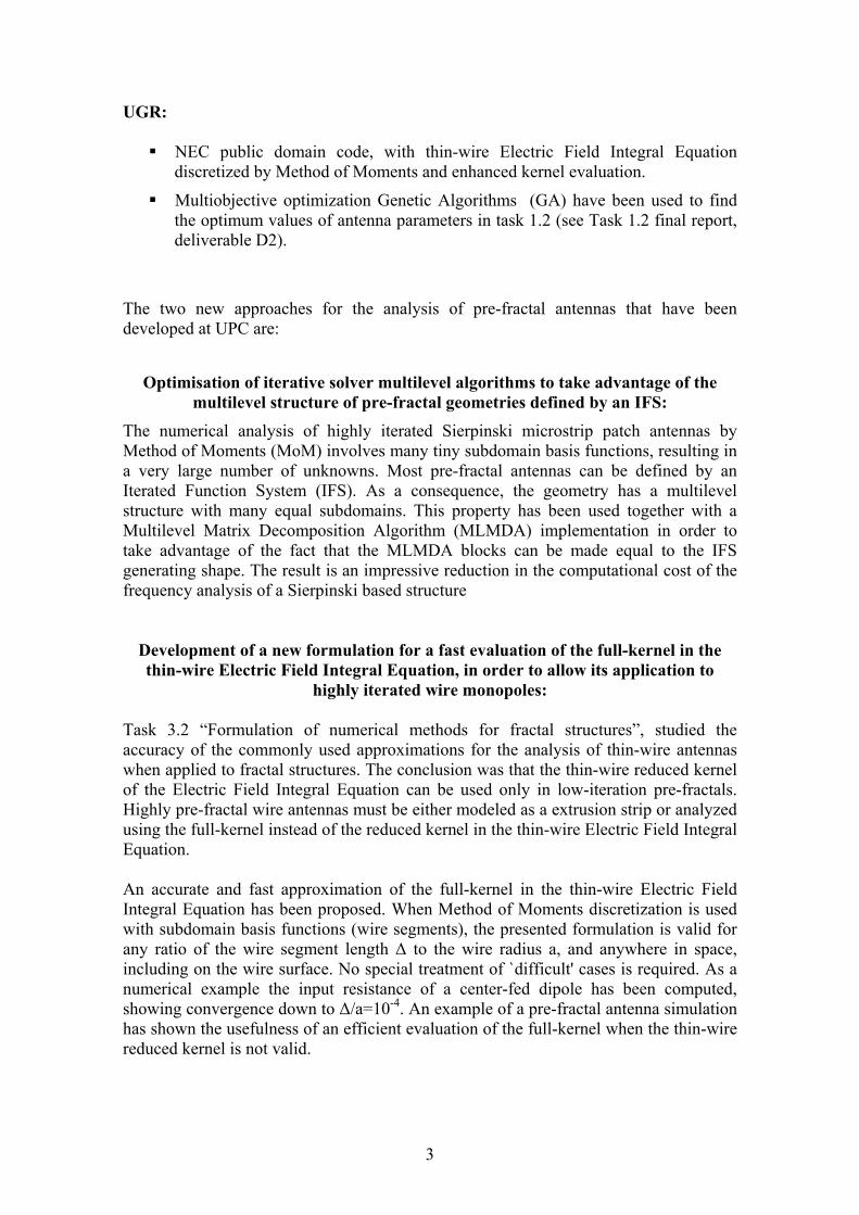
1 2q q qθ θ θ= = , the IFS transformation is a contractive similarity (angles are preserved) where rq is the scale factor and θq is the rotation angle. The column matrix tq is just a translation on the plane. Fig. 1 shows the Sierpinski fractal obtained from a single triangle after applying a set of transformations recursively. Structures generated by an IFS necessarily have many equal subdomains at different levels. The impedance matrix resulting from MoM discretization has therefore plenty of

5

redundant information, since the interaction between equal pairs of subdomains produces equal submatrices (1A, 2A, 3A in Fig. 2) if the Green’s function has translation symmetry, as is the case here. There are many sets of equal submatrices in [Z] at different levels. The MoM implementation presented here uses the IFS definition in order to avoid recomputation and storage of redundant matrix elements.

2.3. Multilevel algorithms

The electric field integral equation (EFIE) in the frequency domain discretized by MoM may be expressed in matrix form as [3] [9]

]][[][ JZEi =− (2)

where [J] are the coefficients of the induced current discretized in RWG basis functions (unknowns), [Ei] is the discretization of the incident field and [Z] is the impedance matrix. This matrix includes the Green's function with all the information about the multilayer media. The induced current coefficients [J] are found using the Generalized Minimum Residual (GMRES) [4] iterative method. In each iteration, the main computational effort to obtain the kth estimation of the induced current [J(k)] are the matrix-vector products [Z][J(k–1)]. Using direct matrix-vector multiplication, the operation count and the memory requirements for each iteration are proportional to N2.

Fig. 2. Method of moments impedance matrix for a five iteration Sierpinski patch antenna. Greyscale shows the magnitude of the matrix elements. If the structure is generated by an IFS, theimpedance matrix has plenty of redundant information: submatrices 1A, 2A and 3A areidentical. Besides, due to the recursive application of the IFS, each one of these submatrices hasalso redundant information, as shown in B and C.

rq = 0.5, θq = 0 + translation-q

q = 1…3

Fig. 1. Four iteration Sierpinski fractal obtained after a set of affine transformations.

rq = 0.5, θq = 0 + translation-q

q = 1…3

rq = 0.5, θq = 0 + translation-q

q = 1…3

6

2.4. Multilevel subdivision of the object

In order to reduce the operation count in the direct matrix-vector multiplication from N2 to N log N, the MLMDA and the MLFMA divide the object into an octal tree in 3D or a quad tree in 2D containing many non-overlaping subdomains or boxes. The quad tree domain subdivision that is generally used for arbitrary structures is applied here to a Sierpkinski fractal in Fig. 3a. The interaction between a pair of subdomains can be computed as

]][[][ nmnm JZE = (3)

where n and m, respectively, are the indexes of the RWG basis functions in the source and observation subdomains and [Zmn] is a submatrix of the impedance matrix. If all possible pairs of subdomains are considered, the matrix vector multiplication [Z][J(k–1)] may be obtained as the addition of submatrix operations of the form (3).

2.5. The multilevel matrix decomposition algorithm (MLMDA).

The MLMDA will be only outlined here, more details can be found in [8]. It consists of a recursive procedure that begins at level 2 and stops at the finest level L. For each non-empty source and observation boxes which belong to the same subdivision level l (2 ≤ l ≤ L) there are two possible cases:

1. Boxes are touching one another or are the same: then they are subdivided into level l+1 boxes, except if we have already reached the finest level, l=L. If this is the case, direct submatrix-vector multiplication (3) is performed, requiring the previous computation of the corresponding matrix terms of [Zmn]. Time and memory requirements are proportional to MbNb where Mb and Nb are the number of original RWG functions in the source and observation box, respectively.

2. Boxes are not touching each other: In this case, the number of degrees of Freedom (DoF) of the electric field [Em] at the observation box in (3) is smaller than Nb, and decreases for larger box-to-box distance and for smaller box size [7] [8]. Therefore, [Em] in (3) can be computed very efficiently in much less than MbNb operations by replacing the original currents by a very small set of equivalent ones that radiate the same field.

7

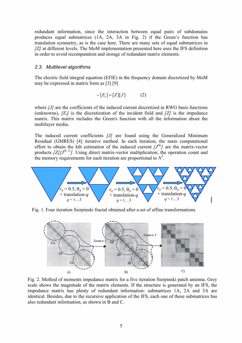
The computational cost of this recursive algorithm increases with the number of non-empty boxes in the multilevel subdivision of a given object. If we realize that, for a IFS generated fractal, boxes do not need to be square as in Fig. 3a, while they do not overlap and cover the whole geometry of the antenna, we can use boxes of the same shape and size as the IFS building blocks (Fig. 3b). For the case of the Sierpinski antenna triangular boxes are the optimum choice. This results in a multilevel subdivision with: many empty boxes and many pairs of source and field boxes having the same interaction matrices either in step 1 or in the equivalent source formulation of step 2. These matrices will be computed once, stored in memory and reused whenever required, leading to a dramatic reduction in computation time and memory storage.

2.6. Results

Configurations of a microstrip Sierpinski patch antenna with four, five, six, and seven iterations have been used as a benchmark in order to test different approaches to enhance the MoM analysis. In all the cases the scale factor is 2 and the height of the equilateral triangle defining the Sierpinski patch (level 1 in Fig. 3) is 8.89 cm. The dielectric substrate is 1.57 mm thick with a relative permitivity of 2.33. The patch was excited with a standard coaxial probe located in the lower corner of the Sierpinski fractal. The computer used in the simulation is a desktop PC with an AMD Athlon CPU at 1.33 GHz and 1.5 GB of RAM. The programming language is MATLAB 6 with time-critical routines coded in C language. Table I shows the computational requirements for the solution of the MoM linear system (2) using direct matrix inversion. Memory requirements grow as N2 and time as N3, as expected. For the seven iteration configuration, the storage requirements overcome the available memory. In table II the same test is repeated using GMRES instead of the direct inversion. Preconditioning is used to reduce the number of iterations [4]. The preconditioner is a sparse matrix that includes all the impedance matrix elements corresponding to basis and testing functions that are close to each other, and zeros elsewhere. The incomplete

Fig 3. a) Multilevel decomposition for arbitrary shapes. b) Multilevel decomposition for IFSgenerated fractals: while boxes do not overlap and cover the whole geometry of the antenna,they can be of the same size and shape as the IFS building blocks. This decomposition producesmany pairs of source and field boxes with the same interaction matrices.

LEVEL

2

LEVEL

1 LEVEL

3a b)

8

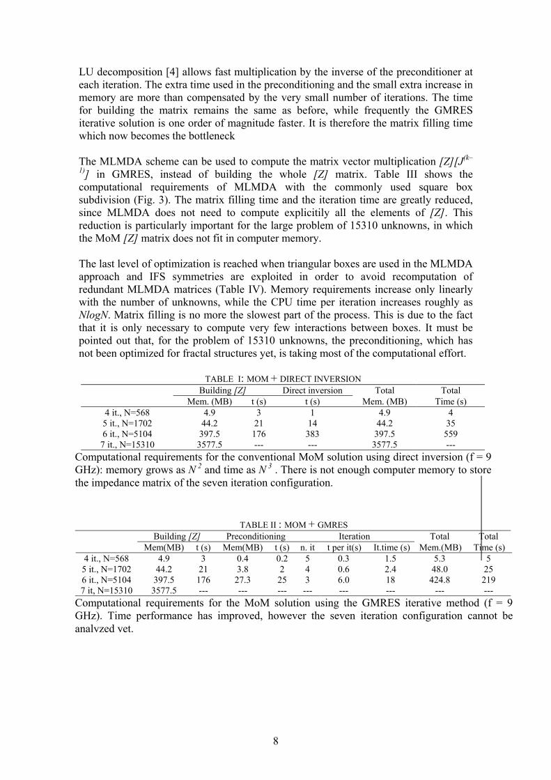
LU decomposition [4] allows fast multiplication by the inverse of the preconditioner at each iteration. The extra time used in the preconditioning and the small extra increase in memory are more than compensated by the very small number of iterations. The time for building the matrix remains the same as before, while frequently the GMRES iterative solution is one order of magnitude faster. It is therefore the matrix filling time which now becomes the bottleneck The MLMDA scheme can be used to compute the matrix vector multiplication [Z][J(k–

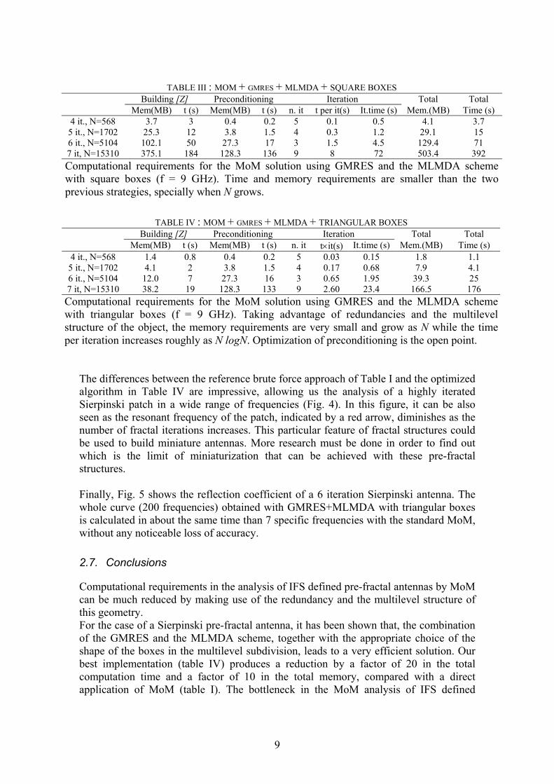
1)] in GMRES, instead of building the whole [Z] matrix. Table III shows the computational requirements of MLMDA with the commonly used square box subdivision (Fig. 3). The matrix filling time and the iteration time are greatly reduced, since MLMDA does not need to compute explicitily all the elements of [Z]. This reduction is particularly important for the large problem of 15310 unknowns, in which the MoM [Z] matrix does not fit in computer memory. The last level of optimization is reached when triangular boxes are used in the MLMDA approach and IFS symmetries are exploited in order to avoid recomputation of redundant MLMDA matrices (Table IV). Memory requirements increase only linearly with the number of unknowns, while the CPU time per iteration increases roughly as NlogN. Matrix filling is no more the slowest part of the process. This is due to the fact that it is only necessary to compute very few interactions between boxes. It must be pointed out that, for the problem of 15310 unknowns, the preconditioning, which has not been optimized for fractal structures yet, is taking most of the computational effort.

TABLE II : MOM + GMRES Building [Z] Preconditioning Iteration Total Total Mem(MB) t (s) Mem(MB) t (s) n. it t per it(s) It.time (s) Mem.(MB) Time (s)

4 it., N=568 4.9 3 0.4 0.2 5 0.3 1.5 5.3 5 5 it., N=1702 44.2 21 3.8 2 4 0.6 2.4 48.0 25 6 it., N=5104 397.5 176 27.3 25 3 6.0 18 424.8 219 7 it, N=15310 3577.5 --- --- --- --- --- --- --- ---

Computational requirements for the MoM solution using the GMRES iterative method (f = 9 GHz). Time performance has improved, however the seven iteration configuration cannot be analyzed yet.

TABLE I: MOM + DIRECT INVERSION Building [Z] Direct inversion Total Total Mem. (MB) t (s) t (s) Mem. (MB) Time (s)

4 it., N=568 4.9 3 1 4.9 4 5 it., N=1702 44.2 21 14 44.2 35 6 it., N=5104 397.5 176 383 397.5 559

7 it., N=15310 3577.5 --- --- 3577.5 --- Computational requirements for the conventional MoM solution using direct inversion (f = 9 GHz): memory grows as N 2 and time as N 3 . There is not enough computer memory to store the impedance matrix of the seven iteration configuration.

9

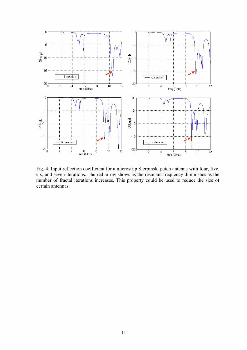
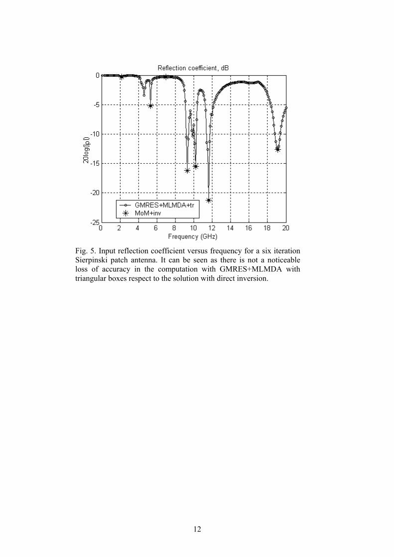
The differences between the reference brute force approach of Table I and the optimized algorithm in Table IV are impressive, allowing us the analysis of a highly iterated Sierpinski patch in a wide range of frequencies (Fig. 4). In this figure, it can be also seen as the resonant frequency of the patch, indicated by a red arrow, diminishes as the number of fractal iterations increases. This particular feature of fractal structures could be used to build miniature antennas. More research must be done in order to find out which is the limit of miniaturization that can be achieved with these pre-fractal structures. Finally, Fig. 5 shows the reflection coefficient of a 6 iteration Sierpinski antenna. The whole curve (200 frequencies) obtained with GMRES+MLMDA with triangular boxes is calculated in about the same time than 7 specific frequencies with the standard MoM, without any noticeable loss of accuracy.

2.7. Conclusions

Computational requirements in the analysis of IFS defined pre-fractal antennas by MoM can be much reduced by making use of the redundancy and the multilevel structure of this geometry. For the case of a Sierpinski pre-fractal antenna, it has been shown that, the combination of the GMRES and the MLMDA scheme, together with the appropriate choice of the shape of the boxes in the multilevel subdivision, leads to a very efficient solution. Our best implementation (table IV) produces a reduction by a factor of 20 in the total computation time and a factor of 10 in the total memory, compared with a direct application of MoM (table I). The bottleneck in the MoM analysis of IFS defined

TABLE III : MOM + GMRES + MLMDA + SQUARE BOXES Building [Z] Preconditioning Iteration Total Total Mem(MB) t (s) Mem(MB) t (s) n. it t per it(s) It.time (s) Mem.(MB) Time (s)

4 it., N=568 3.7 3 0.4 0.2 5 0.1 0.5 4.1 3.7 5 it., N=1702 25.3 12 3.8 1.5 4 0.3 1.2 29.1 15 6 it., N=5104 102.1 50 27.3 17 3 1.5 4.5 129.4 71 7 it, N=15310 375.1 184 128.3 136 9 8 72 503.4 392 Computational requirements for the MoM solution using GMRES and the MLMDA scheme with square boxes (f = 9 GHz). Time and memory requirements are smaller than the two previous strategies, specially when N grows.

TABLE IV : MOM + GMRES + MLMDA + TRIANGULAR BOXES Building [Z] Preconditioning Iteration Total Total Mem(MB) t (s) Mem(MB) t (s) n. it t×it(s) It.time (s) Mem.(MB) Time (s)

4 it., N=568 1.4 0.8 0.4 0.2 5 0.03 0.15 1.8 1.1 5 it., N=1702 4.1 2 3.8 1.5 4 0.17 0.68 7.9 4.1 6 it., N=5104 12.0 7 27.3 16 3 0.65 1.95 39.3 25 7 it, N=15310 38.2 19 128.3 133 9 2.60 23.4 166.5 176 Computational requirements for the MoM solution using GMRES and the MLMDA scheme with triangular boxes (f = 9 GHz). Taking advantage of redundancies and the multilevel structure of the object, the memory requirements are very small and grow as N while the time per iteration increases roughly as N logN. Optimization of preconditioning is the open point.

10

geometries is now in the preconditioning, which has not been optimized for IFS structures yet. It has been observed, through numerical experiments, that the resonant frequency of the Sierpinski patch diminishes as the number of fractal iterations of the geometry increases. This feature can be used to build miniature antennas, however more research must be done in order to find out which are the limits for these pre-fractal structures.

2.8. References

[1] C. Puente, J. Romeu, R. Pous, X. García, F. Benitez, "Fractal multiband antenna based on the Sierpinski gasket", Electronic letters, vol. 32, nº 1, pp. 1-2, January 1996. [2] C. Puente, J. Romeu, R. Pous, A. Cardama, "On the behavior of the Sierpinski multiband antenna", IEEE Transactions on Antennas and Propagation, vol. 46, nº 4, pp. 517-524, April 1998. [3] R. F. Harington, Field Computation by Moment Methods, MacMillan, 1968. [4] Y. Saad, Iterative Methods for Sparse Linear Systems, PWS Publishing Company, Boston, 1996 [5] R. Coifman, V. Rohklin, and S. Wandzura, "The fast multipole method for the wave equation: a pedestrian description", IEEE Transactions on Antennas and Propagation, vol. 35, pp. 7-12, 1993. [6] J. Song, C. C. Lu, W. C. Chew, "Multilevel fast multipole algorithm for electromagnetic scattering by large complex objects", IEEE Transactions on Antennas and Propagation, vol. 45, pp. 1488-1493, 1997. [7] E. Michelsen, A. Boag, "A multilevel matrix decomposition algorithm for analyzing scattering from large structures", IEEE Transactions on Antennas and Propagation, vol. 44, pp. 1086-1093, 1996. [8] J. Parrón, J. M. Rius, J. R. Mosig, " Application of the Multilevel Matrix Decomposition Algorithm to the Frequency Analysis of Large Microstrip Antenna Arrays" IEEE Transactions on Magnetics, scheduled for March 2002. [9] S. M. Rao, D. R. Wilton, A. W. Glisson, "Electromagnetic scattering by surfaces of arbitrary shape", IEEE Transactions on Antennas and Propagation, vol 30, pp. 409-419, 1982.. [10] H. O. Pietgen, H. Jurgerns, , D. Saupe, Chaos and Fractals, New Frontiers in Science, Springer Verlag, New York, 1992

11

Fig. 4. Input reflection coefficient for a microstrip Sierpinski patch antenna with four, five,six, and seven iterations. The red arrow shows as the resonant frequency diminishes as thenumber of fractal iterations increases. This property could be used to reduce the size ofcertain antennas.

12

Fig. 5. Input reflection coefficient versus frequency for a six iteration Sierpinski patch antenna. It can be seen as there is not a noticeableloss of accuracy in the computation with GMRES+MLMDA withtriangular boxes respect to the solution with direct inversion.

3 Efficient Full-Kernel Evaluation in the Thin-

Wire Electric Field Integral Equation

3.1 Introduction

The thin wire model in computational electromagnetics is used for problems thatcan be modeled as a set of electrically thin cylinders, referred to as wire segments.The wire segments are assumed to be sufficiently thin for the following conditionsto hold:

1. Only the axial components of the induced surface current and the incidentfield need to be considered.

2. Both the induced surface current and the incident field are constant along thewire circumference.

Under these conditions, the surface current can be expanded in one-dimensionallocal basis functions for use in the Method of Moments (MoM) [1]. In the MoM, themutual impedances of all the wire segments must be evaluated. This involves theintegration of the basis functions and their divergence over the wire surface, with akernel given by the appropriate Green’s function.

If the wire radius a is small compared to the segment length ∆, then an efficientevaluation of this integral is possible using an approximation of the Green’s functioncalled the reduced kernel or thin wire approximation [2],[3]. However, there are someproblems of practical interest, like highly iterated fractal antennas, in which themodel contains short and thick segments, and therefore the thin-wire approximationcannot be rigorously applied.

On the other hand, the integral with the full kernel is valid for any segmentlength / radius ratio, but it has no analytical solution and solving it by numericalintegration is computationally expensive, particularly for the self-impedance of thewire segments, for which the kernel is singular. Several approaches have been pre-sented in literature for the evaluation of the full kernel. The series approach in [4]and the extended kernel of the well known computer program NEC-2 [5] are limitedto ∆/a > 2. More recently, series representations have been presented that are validwithout restrictions on ∆/a [6],[7],[8]. However, for small ∆/a these series showslow convergence.

In this report, a new formulation is presented, that allows a very fast evaluationof the full kernel, even for ∆/a ¿ 1, including the usually difficult case of theself-impedance term .

3.2 Cylindrical (or Full-) Wire Kernel

The MoM solution of radiation and scattering problems for Perfectly Conducting(PEC) wires is based on a formulation of the problem in terms of the Electric Field

13

Integral Equation (EFIE), given by

bn×−→E i(−→r ) = bn× jη

4πk

³−→A (−→r ) +∇Φ(−→r )

´(1)

in which −→r is any point on the object surface, bn is the outward surface normal atthat point,

−→E i is the imposed incident electric field (excitation),

−→A (−→r ) = k2

ZS

−→J (~r0)

e−jkR

Rds, R = |−→r −−→r 0| (2)

the vector potential due to the surface current distribution−→J over the entire problem

surface S, and

Φ(−→r ) =ZS

σ (~r0)e−jkR

Rds, R = |−→r −−→r 0| (3)

the scalar potential due to the surface charge density σ.

The common approach for thin-wire models, with a¿ λ, is to assume the currentand charge densities to be constant along the wire segment circumference. Then, thesurface current and charge density distributions reduce to, respectively, a currentdistribution Iz(z) and a line charge q(z), defined through

−→J (z,φ) =

1

2πaIz(z)buz (4)

and

σ =j

ω∇s ·−→J = j

2πωa

dIz(z)

dz=

1

2πaq(z) (5)

where we assume the wire segment to be aligned with the z-axis. The potentialsthen become −→

A (−→r ) = k2Z`

Iz(z0)G(R)buz0dz0 (6)

and

Φ(−→r ) =Z`

q(z0)G(R)dz0 (7)

whereG(R) is a Greens’ function incorporating the circumferential integration, givenby

G(R) =

Z 2π

0

1

2π

e−jkR

Rdφ0 R = |−→r −−→r 0| (8)

Eq. (8) is known as the cylindrical wire kernel —or full-kernel of the thin-wire EFIE—.

In the MoM, the current and charge are expanded into basis functions definedon the wire model. The technique presented in this report uses an expansion of thecurrent into bilinear or triangle basis functions [9]. The domain of a basis functionconsists of two adjacent segments. Its value equals one at the joint vertex and dropslinearly to zero at the outer vertices. Consequently, the charge is piecewise constant.

The EFIE (1) is weighted by the same triangle basis functions used to expandthe current, along a line on the wire surface parallel to the axis. The weightingprocedure is not critical and can be done using a one-point integration scheme (atthe center of the segments). The problem at hand therefore consists in the evaluationof (6) and (7), for all wire segment centers, by integrating over all two-segment basisfunction surfaces.

14

O

z

p

r’

rp

zp

z=∆

ab

O

z

pp

r’r’

rp

zp

z=∆

ab

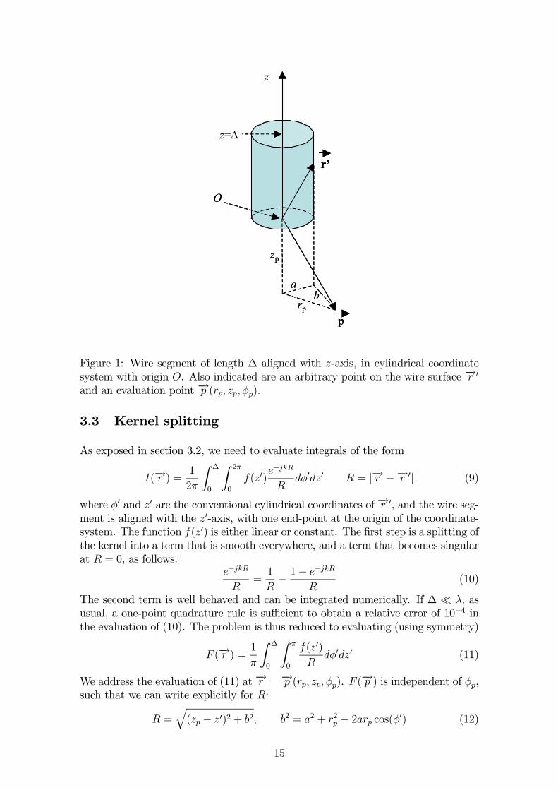
Figure 1: Wire segment of length ∆ aligned with z-axis, in cylindrical coordinatesystem with origin O. Also indicated are an arbitrary point on the wire surface −→r 0and an evaluation point −→p (rp, zp,φp).

3.3 Kernel splitting

As exposed in section 3.2, we need to evaluate integrals of the form

I(−→r ) = 1

2π

Z ∆

0

Z 2π

0

f(z0)e−jkR

Rdφ0dz0 R = |−→r −−→r 0| (9)

where φ0 and z0 are the conventional cylindrical coordinates of −→r 0, and the wire seg-ment is aligned with the z0-axis, with one end-point at the origin of the coordinate-system. The function f(z0) is either linear or constant. The first step is a splitting ofthe kernel into a term that is smooth everywhere, and a term that becomes singularat R = 0, as follows:

e−jkR

R=1

R− 1− e

−jkR

R(10)

The second term is well behaved and can be integrated numerically. If ∆ ¿ λ, asusual, a one-point quadrature rule is sufficient to obtain a relative error of 10−4 inthe evaluation of (10). The problem is thus reduced to evaluating (using symmetry)

F (−→r ) = 1

π

Z ∆

0

Z π

0

f(z0)R

dφ0dz0 (11)

We address the evaluation of (11) at −→r = −→p (rp, zp,φp). F (−→p ) is independent of φp,such that we can write explicitly for R:

R =q(zp − z0)2 + b2, b2 = a2 + r2p − 2arp cos(φ0) (12)

15

recalling that a is the wire segment radius and b as depicted in Fig. 1.

It is easily shown, that for f(z0) linear:

Flin(zp, rp,∆, a) = aFlin(zp/a, rp/a,∆/a, 1) (13)

and for f(z0) constant

Fcon(zp, rp,∆, a) = Fcon(zp/a, rp/a,∆/a, 1) (14)

so we can always scale the problem with respect to a and be left with an expres-sion that depends only on zp, rp and ∆. From here on, the scaling is implicit, fornotational simplicity. Using a change of variable

u0 = z0 − zp, (15)

we can immediately see

Fcon(zp, rp,∆) = Fcon(0, rp,∆+ |zp|)− Fcon(0, rp, |zp|) (16)

which yields an expression for Fcon with two terms that depend on two variablesonly. For arbitrary values of r and ∆, we define these as

Fcon(r,∆) ≡ Fcon(0, r,∆) (17)

For Flin the situation is slightly more complicated. Fig. 2 illustrates the procedure.The change of variable (15) yields

Flin(zp, rp,∆) = Flin(0, rp,∆+ |zp|)− Flin(0, rp, |zp|)−|zp|Fcon(zp, rp,∆) (18)

Again we have an expression with two terms that depend on two variables only, andone term (the third) that is already known from (16). We define, for arbitrary r and∆,

Flin(r,∆) ≡ Flin(0, r,∆)In the thin wire approximation (valid for∆À 1, see section 3), these two expressionsare given by

Fcon(r,∆) ≈ lnµq

(∆/r)2 + 1 +∆/r

¶(19)

andFlin(r,∆) ≈

√∆2 + r2 (20)

In the next section we present new expressions that do not use the thin wire ap-proximation and are valid for all r ≥ 1,∆ > 0.

3.4 Approximations

3.4.1 Constant integrand

The integrals to be evaluated for the case with f(z0) constant are of the form

Fcon(r,∆) =1

π

Z ∆

0

Z π

0

1√z02 + b2

dφ0dz0 (21)

16

z

r

f(z)=z-zpz=∆

z=0

z=zp, u=0

r=0 r=|zp|

P(rp,zp)

(B)

(A)

(C)

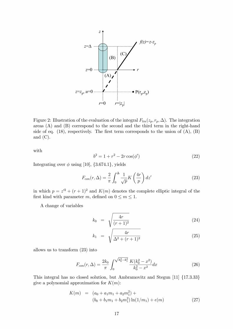
Figure 2: Illustration of the evaluation of the integral Flin(zp, rp,∆). The integrationareas (A) and (B) correspond to the second and the third term in the right-handside of eq. (18), respectively. The first term corresponds to the union of (A), (B)and (C).

withb2 = 1 + r2 − 2r cos(φ0) (22)

Integrating over φ using [10], 3.674.1, yields

Fcon(r,∆) =2

π

Z ∆

0

1√pK

µ4r

p

¶dz0 (23)

in which p = z02 + (r + 1)2 and K(m) denotes the complete elliptic integral of thefirst kind with parameter m, defined on 0 ≤ m ≤ 1.A change of variables

k0 =

s4r

(r + 1)2(24)

k1 =

s4r

∆2 + (r + 1)2(25)

allows us to transform (23) into

Fcon(r,∆) =2k0π

Z √k20−k210

K(k20 − x2)k20 − x2

dx (26)

This integral has no closed solution, but Ambramovitz and Stegun [11] 17.3.33give a polynomial approximation for K(m):

K(m) = (a0 + a1m1 + a2m21) +

(b0 + b1m1 + b2m21) ln(1/m1) + ²(m) (27)

17

0 0.1 0.2 0.3 0.4 0.5 0.6 0.7 0.8 0.9 110-6

10-5

10-4

m

rela

tive

erro

r

series approx of K(m)/m

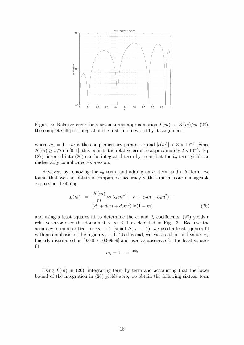
Figure 3: Relative error for a seven terms approximation L(m) to K(m)/m (28),the complete elliptic integral of the first kind devided by its argument.

where m1 = 1 −m is the complementary parameter and |²(m)| < 3 × 10−5. SinceK(m) ≥ π/2 on [0, 1], this bounds the relative error to approximately 2× 10−5. Eq.(27), inserted into (26) can be integrated term by term, but the b0 term yields anundesirably complicated expression.

However, by removing the b0 term, and adding an a3 term and a b3 term, wefound that we can obtain a comparable accuracy with a much more manageableexpression. Defining

L(m) =K(m)

m≈ (c0m−1 + c1 + c2m+ c3m2) +

(d0 + d1m+ d2m2) ln(1−m) (28)

and using a least squares fit to determine the ci and di coefficients, (28) yields arelative error over the domain 0 ≤ m ≤ 1 as depicted in Fig. 3. Because theaccuracy is more critical for m → 1 (small ∆, r → 1), we used a least squares fitwith an emphasis on the region m→ 1. To this end, we chose a thousand values xi,linearly distributed on [0.00001, 0.99999] and used as abscissae for the least squaresfit

mi = 1− e−10xi

Using L(m) in (26), integrating term by term and accounting that the lowerbound of the integration in (26) yields zero, we obtain the following sixteen term

18

1 2 3 4 5 6 7 8 9 1010-6

10-5

10-4

r/a

rela

tive

erro

r

16-term approximation of F con

∆=0.1a∆=1a∆=10a

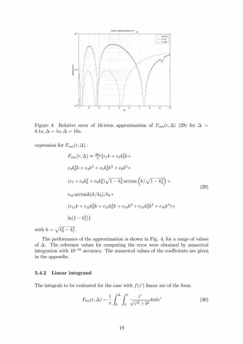
Figure 4: Relative error of 16-term approximation of Fcon(r,∆) (29) for ∆ =0.1a,∆ = 1a,∆ = 10a.

expression for Fcon(r,∆) :

Fcon(r,∆) ≈ 2k0πe1k + e2k20k+

e3k40k + e4k

3 + e5k20k3 + e6k

5+

(e7 + e8k20 + e9k

40)p1− k20 arctan

³k/p1− k20

´+

e10 arctanh(k/k0)/k0+

(e11k + e12k20k + e13k

40k + e14k

3 + e15k20k3 + e16k

5)×

ln(1− k21)

(29)

with k =pk20 − k21.

The performance of the approximation is shown in Fig. 4, for a range of valuesof ∆. The reference values for computing the error were obtained by numericalintegration with 10−10 accuracy. The numerical values of the coefficients are givenin the appendix.

3.4.2 Linear integrand

The integrals to be evaluated for the case with f(z0) linear are of the form

Flin(r,∆) =1

π

Z ∆

0

Z π

0

z0√z02 + b2

dφdz0 (30)

19

with b as in (22). The integration over z0 is elementary, leading to

Flin(r,∆) =1

π

Z π

0

³√∆2 + b2 − b

´dφ (31)

Using [10] 2.576, (31) can be solved yielding

Flin(r,∆) =2

π

½ p(1 + r)2 +∆2E(k21)−(1 + r)E(k20)

¾(32)

with k0, k1 given by (24) and (25). Since the second term in (32) does not dependon ∆, it is cancelled out between the two terms in (18), so in practise it is nevercomputed. E(m) represents the complete elliptic integral of the second kind, definedon 0 ≤ m ≤ 1 (recall that 0 ≤ k0 ≤ 1 and 0 ≤ k1 ≤ 1).Abramovitz and Stegun [11], 17.3.35 give a polynomial approximation for

E(m):

E(m) ≈ (1 + f1m1 + f2m21) + (33)

(g1m1 + g2m21) ln(1/m1) + ²(m),

where m1 = 1 −m is the complementary parameter and |²(m)| < 4 × 10−5. SinceE(m) ≥ 1 on [0, 1], the relative error in (33) is also bounded by 4× 10−5.The relative error in (18), however, can be considerably higher because of a can-

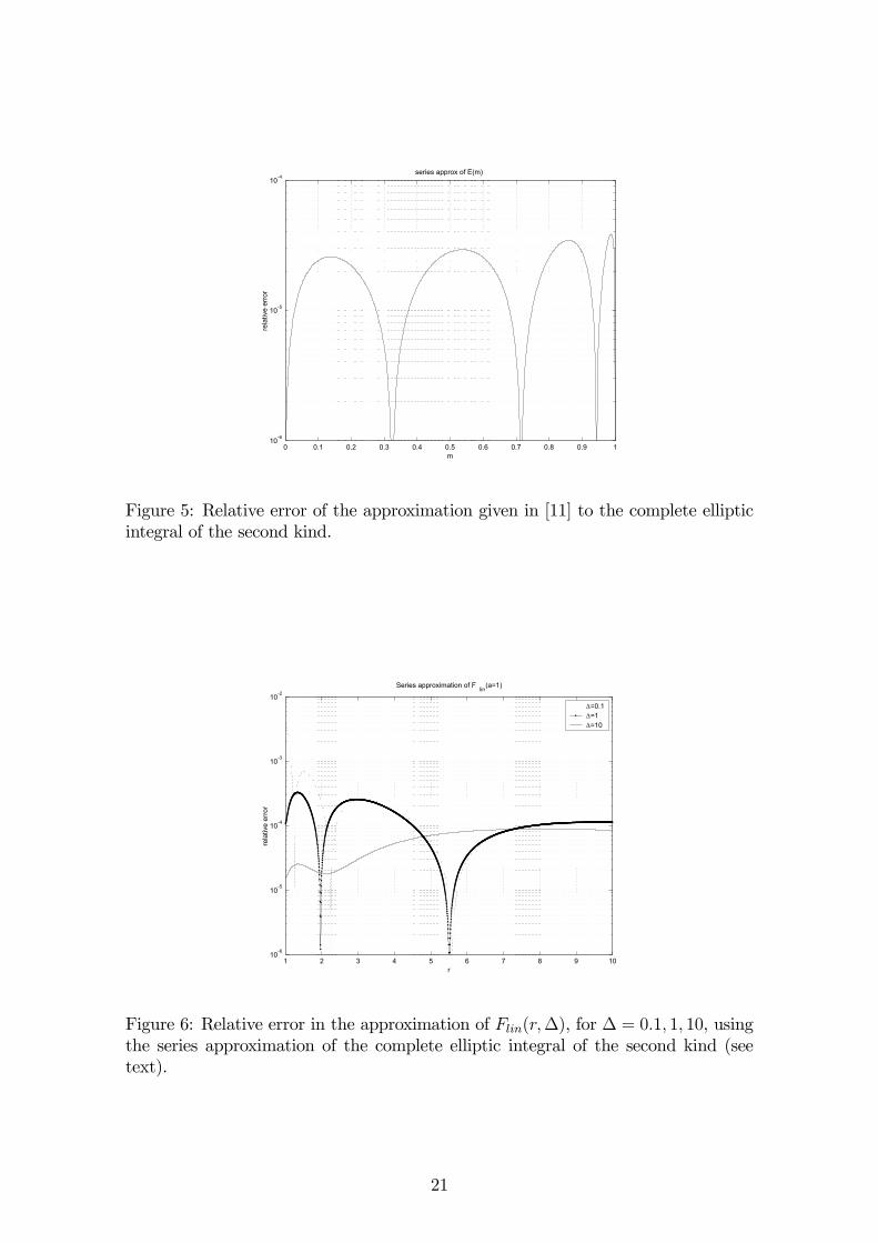
cellation of the two terms in (18), especially for very small values of ∆. Fortunately,in the MoM application presented here, the constant term Fcon(r,∆) is always dom-inant and, therefore, the relative accuracy of the substraction Flin(0, rp,∆+ |zp|)−Flin(0, rp, |zp|) in (18) is not critical.The relative error of the resulting fit (33) is shown in Fig. 5. Using this ap-

proximation, we computed the relative error in Flin(r,∆) for a range of values of ∆.The results are shown in Fig. 6. The reference values for computing the error wereobtained by numerical integration with 10−10 accuracy. The numerical values of thecoefficients are given in the appendix.

3.5 Numerical results

We validated the approximations in section 3.4 by calculating the input impedanceof the half-wave center-fed dipole antenna that was used as an example in [8]. Thecharacteristics of the dipole are: length L = 0.25 λ, radius a = 0.0509 λ. The dipoleis center-fed using the delta gap model with a Gaussian forcing function

Eiz =1√πae−2

(z−zs)2a2

where zs is the z-coordinate of the feeding gap on a z-oriented wire-segment [9].

The calculations were done using the thin wire approximation and using theapproach presented in this report (labeled full kernel in the figure). The result, asa function of ∆/a, is shown in Fig. 7.

20

0 0.1 0.2 0.3 0.4 0.5 0.6 0.7 0.8 0.9 110-6

10-5

10-4

m

rela

tive

erro

r

series approx of E(m)

Figure 5: Relative error of the approximation given in [11] to the complete ellipticintegral of the second kind.

1 2 3 4 5 6 7 8 9 1010-6

10-5

10-4

10-3

10-2

r

rela

tive

erro

r

Series approximation of F lin(a=1)

∆=0.1∆=1∆=10

Figure 6: Relative error in the approximation of Flin(r,∆), for ∆ = 0.1, 1, 10, usingthe series approximation of the complete elliptic integral of the second kind (seetext).

21

10-3 10-2 10-1 100-100

-50

0

50

100

150

∆/a

Z in (Ω

)

Input Impedance, 0.5 λ dipole, radius 0.0509 λ

Real

Imag

thin wire kernelfull kernel

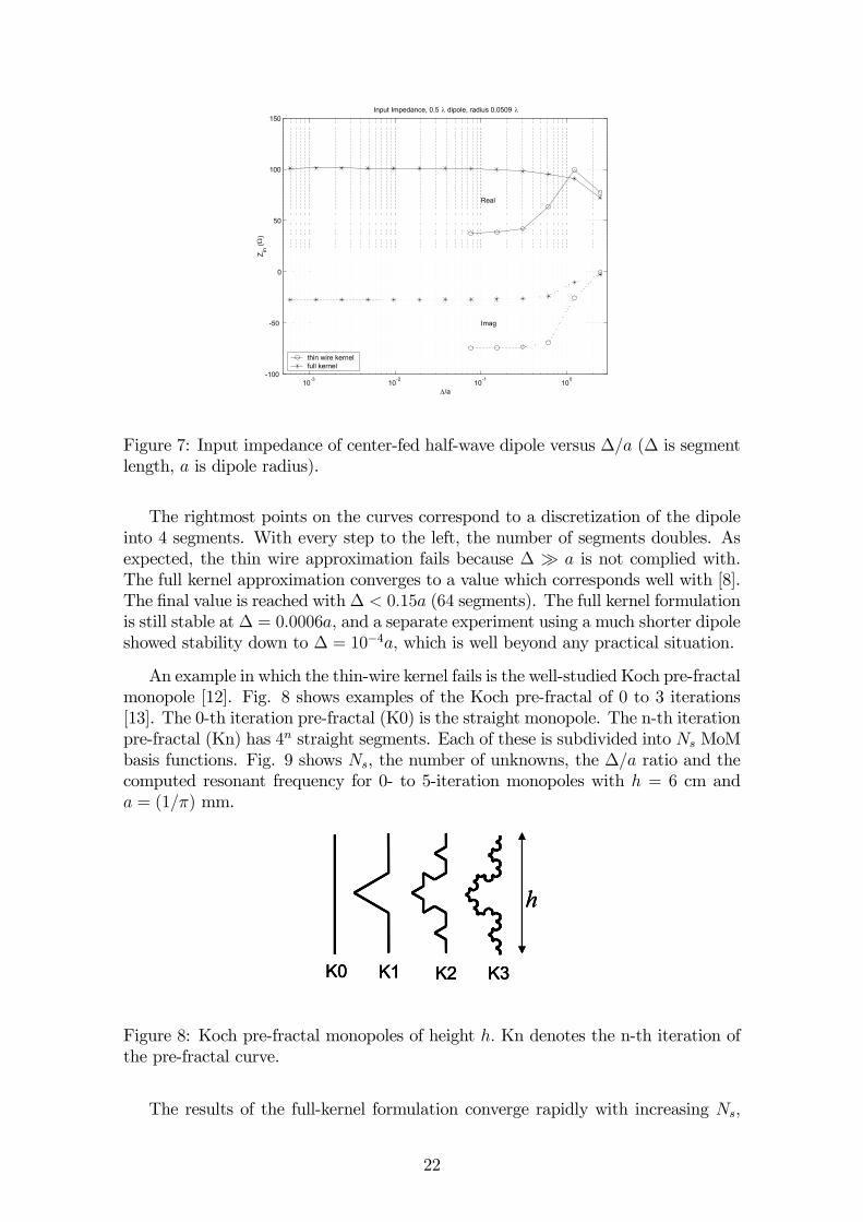
Figure 7: Input impedance of center-fed half-wave dipole versus ∆/a (∆ is segmentlength, a is dipole radius).

The rightmost points on the curves correspond to a discretization of the dipoleinto 4 segments. With every step to the left, the number of segments doubles. Asexpected, the thin wire approximation fails because ∆ À a is not complied with.The full kernel approximation converges to a value which corresponds well with [8].The final value is reached with∆ < 0.15a (64 segments). The full kernel formulationis still stable at ∆ = 0.0006a, and a separate experiment using a much shorter dipoleshowed stability down to ∆ = 10−4a, which is well beyond any practical situation.

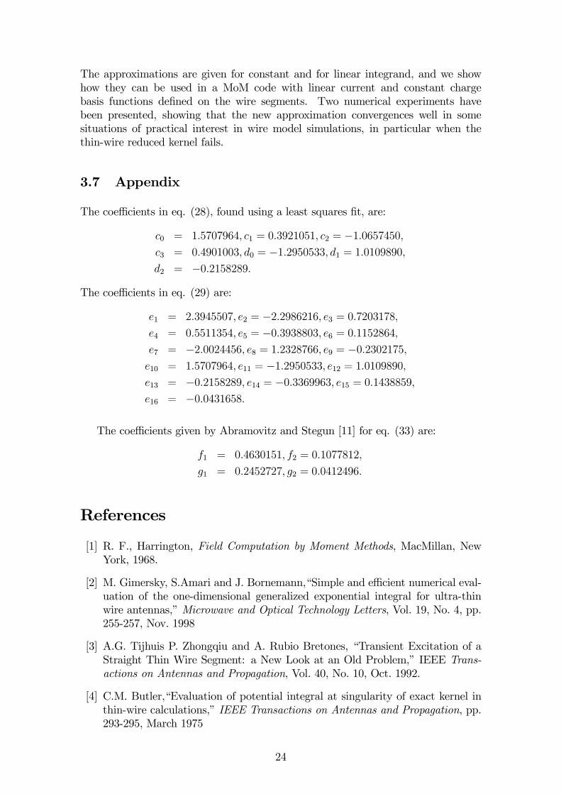
An example in which the thin-wire kernel fails is the well-studied Koch pre-fractalmonopole [12]. Fig. 8 shows examples of the Koch pre-fractal of 0 to 3 iterations[13]. The 0-th iteration pre-fractal (K0) is the straight monopole. The n-th iterationpre-fractal (Kn) has 4n straight segments. Each of these is subdivided into Ns MoMbasis functions. Fig. 9 shows Ns, the number of unknowns, the ∆/a ratio and thecomputed resonant frequency for 0- to 5-iteration monopoles with h = 6 cm anda = (1/π) mm.

K0 K1 K2 K3

h

K0K0 K1K1 K2K2 K3K3

hh

Figure 8: Koch pre-fractal monopoles of height h. Kn denotes the n-th iteration ofthe pre-fractal curve.

The results of the full-kernel formulation converge rapidly with increasing Ns,

22

Ns Unknowns ∆/a Thin-wire Full-kernel15 15 12.57 1.191 1.19130 30 6.28 1.187 1.18760 60 3.14 1.185 1.185

121 121 1.56 1.183 1.184243 243 0.78 1.181 1.183486 486 0.39 1.180 1.183972 972 0.19 1.179 1.1831944 1944 0.10 1.178 1.18310 40 6.28 1.001 1.00120 80 3.14 1.001 1.00140 160 1.56 0.999 1.00081 324 0.78 0.998 1.000

162 648 0.39 0.997 0.999324 1296 0.19 0.995 0.99913 208 1.56 0.894 0.89527 432 0.78 0.893 0.89454 864 0.39 0.888 0.8949 576 0.78 0.848 0.84918 1152 0.39 0.846 0.84936 2304 0.19 0.840 0.8493 768 0.78 0.840 0.8426 1536 0.39 0.836 0.84012 3072 0.19 0.830 0.8401 1024 0.78 0.877 0.8362 2048 0.39 0.849 0.8394 4096 0.19 0.829 0.838

K3

K4

K5

Resonant freq. (GHz)

K0

K1

K2

Ns Unknowns ∆/a Thin-wire Full-kernel15 15 12.57 1.191 1.19130 30 6.28 1.187 1.18760 60 3.14 1.185 1.185

121 121 1.56 1.183 1.184243 243 0.78 1.181 1.183486 486 0.39 1.180 1.183972 972 0.19 1.179 1.1831944 1944 0.10 1.178 1.18310 40 6.28 1.001 1.00120 80 3.14 1.001 1.00140 160 1.56 0.999 1.00081 324 0.78 0.998 1.000

162 648 0.39 0.997 0.999324 1296 0.19 0.995 0.99913 208 1.56 0.894 0.89527 432 0.78 0.893 0.89454 864 0.39 0.888 0.8949 576 0.78 0.848 0.84918 1152 0.39 0.846 0.84936 2304 0.19 0.840 0.8493 768 0.78 0.840 0.8426 1536 0.39 0.836 0.84012 3072 0.19 0.830 0.8401 1024 0.78 0.877 0.8362 2048 0.39 0.849 0.8394 4096 0.19 0.829 0.838

K3

K4

K5

Resonant freq. (GHz)

K0

K1

K2

Figure 9: Resonant frequency for Koch pre-fractal monopoles of 0 to 5 iterations(K0 to K5). K0 corresponds to the straight monopole. Ns denotes the number ofMoM segments in each pre-fractal curve segment.

while the thin-wire reduced kernel does not. For the 5-iteration monopole, evenwith Ns = 1 we have ∆/a < 1, which invalidates the thin-wire reduced kernel. Theradiation resistance Rr at the resonant frequency for the K5 monopole and Ns = 4is:

Formulation Rr resFull-kernel 18.1 ΩThin-wire 0.07 Ω

Although the resonant frequency value computed with the thin-wire reducedkernel has a relative error of about 1%, the radiation resistance is clearly incorrect,which shows the usefulness of an efficient full-kernel computation for the analysis ofpre-fractal antennas.

Regarding the computational efficiency, in our implementation the full kernelis approximately a factor 2 slower than the thin wire kernel. For larger problems,this factor can be improved to approximately one by using the full kernel only tocompute the mutual impedances of nearby segments.

3.6 Conclusions

We have proposed here new approximations for the full kernel of the thin wiremodel, valid at arbitrary evaluation points and for any ∆/a, including ∆/a ¿ 1.

23

The approximations are given for constant and for linear integrand, and we showhow they can be used in a MoM code with linear current and constant chargebasis functions defined on the wire segments. Two numerical experiments havebeen presented, showing that the new approximation convergences well in somesituations of practical interest in wire model simulations, in particular when thethin-wire reduced kernel fails.

3.7 Appendix

The coefficients in eq. (28), found using a least squares fit, are:

c0 = 1.5707964, c1 = 0.3921051, c2 = −1.0657450,c3 = 0.4901003, d0 = −1.2950533, d1 = 1.0109890,d2 = −0.2158289.

The coefficients in eq. (29) are:

e1 = 2.3945507, e2 = −2.2986216, e3 = 0.7203178,e4 = 0.5511354, e5 = −0.3938803, e6 = 0.1152864,e7 = −2.0024456, e8 = 1.2328766, e9 = −0.2302175,e10 = 1.5707964, e11 = −1.2950533, e12 = 1.0109890,e13 = −0.2158289, e14 = −0.3369963, e15 = 0.1438859,e16 = −0.0431658.

The coefficients given by Abramovitz and Stegun [11] for eq. (33) are:

f1 = 0.4630151, f2 = 0.1077812,

g1 = 0.2452727, g2 = 0.0412496.

References

[1] R. F., Harrington, Field Computation by Moment Methods, MacMillan, NewYork, 1968.

[2] M. Gimersky, S.Amari and J. Bornemann,“Simple and efficient numerical eval-uation of the one-dimensional generalized exponential integral for ultra-thinwire antennas,” Microwave and Optical Technology Letters, Vol. 19, No. 4, pp.255-257, Nov. 1998

[3] A.G. Tijhuis P. Zhongqiu and A. Rubio Bretones, “Transient Excitation of aStraight Thin Wire Segment: a New Look at an Old Problem,” IEEE Trans-actions on Antennas and Propagation, Vol. 40, No. 10, Oct. 1992.

[4] C.M. Butler,“Evaluation of potential integral at singularity of exact kernel inthin-wire calculations,” IEEE Transactions on Antennas and Propagation, pp.293-295, March 1975

24

[5] G.J.Burke and A.J.Poggio,“Numerical Electromagnetics Code - Method of Mo-ments,” Technical Doc. 116, Naval Ocean Systems Center, San Diego, Jan 1981

[6] D.H. Werner, “An Exact Formulation for the Vector Potential of a CylindricalAntenna with Uniformly Distributed Current and Arbitrary Radius,” IEEETransactions on Antennas and Propagation, Vol. 41, pp. 1009-1018, Aug 1993.

[7] S. Park and C. Balanis,“Efficient Kernel Calculation of Cylindrical Antennas,”IEEE Transactions on Antennas and Propagation, Vol. 43, No. 11, Nov. 1995

[8] D.H. Werner, “A Method of Moments Approach for the Efficient and AccurateModeling of Moderately Thick Cylindrical Wire Antennas,” IEEE Transactionson Antennas and Propagation, Vol. 46, No. 3, March 1998.

[9] G.P. Junker, A.A. Fisch and A.W. Glisson,“A novel Delta Gap Source Modelfor Center Fed Cylindrical Dipoles,” IEEE Transactions on Antennas and Prop-agation, Vol. 43, No. 5, May 1995

[10] Gradshteyn, I. S. and Ryzhik, I. M, “Tables of Integrals, Series, and Products,”6th ed. San Diego, CA: Academic Press, 2000.

[11] Abramowitz, M. and Stegun, I. A. (Eds.). “Handbook of Mathematical Func-tions,” 9th printing. New York: Dover, 1972.

[12] C. Puente, J. Romeu, R. Pous, J. Ramis, A. Hijazo, “Small but long Kochfractal monopole”, IEE Electronics Letters, Vol. 34, No. 1, pp. 9-10, January,1998.

[13] Heinz-Otto Peitgen, et al., Chaos and Fractals: New Frontiers of Science,Springer-Verlag, 1992.

25

26

DISCLAIMER

The work associated with this report has been carried out in accordance with the highest technical standards and the FRACTALCOMS partners have endeavoured to achieve the degree of accuracy and reliability appropriate to the work in question. However since the partners have no control over the use to which the information contained within the report is to be put by any other party, any other such party shall be deemed to have satisfied itself as to the suitability and reliability of the information in relation to any particular use, purpose or application. Under no circumstances will any of the partners, their servants, employees or agents accept any liability whatsoever arising out of any error or inaccuracy contained in this report (or any further consolidation, summary, publication or dissemination of the information contained within this report) and/or the connected work and disclaim all liability for any loss, damage, expenses, claims or infringement of third party rights.