task assignment and scheduling in uav …etd.lib.metu.edu.tr/upload/12619155/index.pdf · task...
TRANSCRIPT
TASK ASSIGNMENT AND SCHEDULING IN UAV MISSION PLANNINGWITH MULTIPLE CONSTRAINTS
A THESIS SUBMITTED TOTHE GRADUATE SCHOOL OF NATURAL AND APPLIED SCIENCES
OFMIDDLE EAST TECHNICAL UNIVERSITY
BY
FATIH SEMIZ
IN PARTIAL FULFILLMENT OF THE REQUIREMENTSFOR
THE DEGREE OF MASTER OF SCIENCEIN
COMPUTER ENGINEERING
SEPTEMBER 2015


Approval of the thesis:
TASK ASSIGNMENT AND SCHEDULING IN UAV MISSION PLANNINGWITH MULTIPLE CONSTRAINTS
submitted by FATIH SEMIZ in partial fulfillment of the requirements for the degree ofMaster of Science in Computer Engineering Department, Middle East TechnicalUniversity by,
Prof. Dr. Gülbin Dural ÜnverDean, Graduate School of Natural and Applied Sciences
Prof. Dr. Adnan YazıcıHead of Department, Computer Engineering
Prof. Dr. Faruk PolatSupervisor, Computer Engineering Dept., METU
Examining Committee Members:
Prof. Dr. Ismail Hakkı TorosluComputer Engineering Department, METU
Prof. Dr. Faruk PolatComputer Engineering Department, METU
Prof. Dr. Göktürk ÜçolukComputer Engineering Department, METU
Assoc. Prof. Dr. Halit OguztüzünComputer Engineering Department, METU
Assist. Prof. Dr. Tansel ÖzyerComputer Engineering Department, TOBB ETU
Date:

I hereby declare that all information in this document has been obtained andpresented in accordance with academic rules and ethical conduct. I also declarethat, as required by these rules and conduct, I have fully cited and referenced allmaterial and results that are not original to this work.
Name, Last Name: FATIH SEMIZ
Signature :
iv

ABSTRACT
TASK ASSIGNMENT AND SCHEDULING IN UAV MISSION PLANNINGWITH MULTIPLE CONSTRAINTS
Semiz, FatihM.S., Department of Computer Engineering
Supervisor : Prof. Dr. Faruk Polat
September 2015, 71 pages
In the recent years, unmanned aerial vehicles (UAVs) have started to be utilized asthe first choice for high risk and long duration tasks, because UAVs are cheaper; theyare hard to be noticed and they can perform long duration missions. Furthermore, theutilization of UAVs ensures to reduce the risk to the human life. Examples of this kindof missions includes signal collection, surveillance and reconnaissance and combatsupport missions. It is valuable to develop a fully autonomous UAV fleet to performthese kinds of tasks when it is needed, because this kind of missions usually start atunexpected times. Other problems which is in the set of high risk and long durationtasks are multiple constraint UAV scheduling, and target assignment problem. In thisproblem, a fleet of UAVs are supposed to traverse a set of target areas within a limitedarea. The targets are only available within certain time windows and need to betraversed promptly. Moreover, for some large target areas multiple UAVs are neededto perform the task. The objective of this problem is to find a complete schedulingand UAV-target assignment that minimizes the total fuel consumption of the UAVs.This problem is a highly critical real time problem and needs to be solved almost inreal-time. Therefore, methods doing exhaustive search are infeasible. Most of themethods in the literature, try to solve this problem by evolutionary approaches. Inthis thesis, we developed an algorithmic method to solve this problem. This methoduses divide and conquer method to solve this problem. In this way, the problem istransformed into a combination of multiple small problems. We designed a method
v

to convert these small problems into transportation problems. Each transportationproblem is solved with simplex algorithm. The method proposed is compared withvarious methods and has been shown to provide fast, acceptably optimal and reliableresults.
Keywords: Unmanned aerial vehicle (UAV), algorithmic solution, UAV schedulingand target assignment, divide and conquer approach, transportation problem
vi
ÖZ
ÇOKLU KISITLAMALAR IÇEREN INSANSIZ HAVA ARAÇLARI ILE GÖREVPLANLAMA PROBLEMINDE ZAMAN PLANLAMASI VE HEDEF
GÖREVLENDIRMESI
Semiz, FatihYüksek Lisans, Bilgisayar Mühendisligi Bölümü
Tez Yöneticisi : Prof. Dr. Faruk Polat
Eylül 2015 , 71 sayfa
Son yıllarda yüksek risk içeren ve uzun zaman gerektiren görevler için insansız havaaraçları (IHA’lar) ilk tercih olarak seçilmeye baslanmıstır. Çünkü IHA’lar ucuz, far-kedilmesi zor ve uzun süreli islere uygun araçlardır. Dahası IHA’ları kullanmak insanhayatının riske atıldıgı durumları azaltmaktadır. Bu tip görevlere örnek olarak sinyaltoplama, kesif ve gözetleme görevleri ve muharebe destek görevleri gösterilebilir. Butip isleri gerektigi zaman yapabilecek tamamen otonom bir IHA filosuna sahip olmakdegerlidir. Çünkü genellikle bu tip görevler beklenmedik zamanlarda baslamaktadır-lar. Yüksek risk içeren ve uzun zaman gerektiren görevlere bir baska örnekte IHA’larile zaman planlaması ve hedef görevlendirmesi problemidir. Bu problemde IHA filosubelirli bir alandaki bir dizi hedef alanını katetmelidir. Hedefler sadece belirli bir za-man aralıgında uygun olup o zaman aralıgı içinde katedilmelidirler. Dahası bazı genisalana yayılmıs hedefleri katetmek için birden fazla IHA gerekmektedir. Bu problemdeamaç IHA’lar için tam bir zaman planlaması ve IHA-hedef görevlendirmesi yapmanınyanı sıra yakıt tüketimini de azaltmaktır. Bu problem oldukça kritik ve gerçek zamanlıbir problemdir ve hızlı bir sekilde çözülmesi gerekmektedir. Bu sebepten dolayı tamkapsamlı arama yapmak bu problem için uygun degildir. Literatürdeki çogu metod,bu problemi evrimsel metodlarla çözmeye çalısmaktadır. Bu tezde biz problemi çö-zebilmek için algoritmik bir metod üretmis durumdayız. Bu metod, problemi çözmek
vii

için böl ve yönet yöntemini kullanmaktadır. Böylece, problem bir çok küçük proble-minin birlesimine dönüstürülmektedir. Biz olusan bu alt problemleri, ulastırma prob-lemlerine çeviren bir dizayn ürettik. Ortaya çıkartılan ulastırma problemleri simplexalgoritması ile çözülmektedir. Önerilen metod bir çok farklı metodla karsılastırılmısolup hızlı, yeterince optimal ve güvenilir sonuçlar ortaya çıkarttıgı görülmüstür.
Anahtar Kelimeler: Insansız hava araçları (IHA), algoritmik çözüm, IHA’lar ile za-man planlaması ve hedef görevlendirmesi, böl ve yönet yöntemi, ulastırma problemi
viii

To my family
ix

ACKNOWLEDGMENTS
I would like to thank my supervisor Professor Faruk Polat for his constant support,guidance and patience. He was the reason for me to start my research on artificialintelligence area and after three years the situation has not changed. He was therewith all his sincerity whenever I needed it. Without his motivational speeches it wouldhave been much harder to achieve this.
Also I would like to thank all of my family members Memnune Sennur Semiz, YasarSemiz, Fatos Semiz Alparslan and her soon to be born baby. They always helped me,gave belief and motivation. I am lucky to have such a family.
Thanks a lot to Doruk Balkan, Fahrican Kosar, Türker Dolapçı who read this docu-ment and helped me to enhance the language of this thesis.
I would like to thank METU Orienteering and Navigation Team, which has been ateam, a family, and means everything to me. If I would have the chance, I wouldwrite the name of the members one by one here.
Thanks Abdullah Dogan for his helps. He was also trying to finish his thesis andworking till the morning was enjoyable with his presence.
Thanks to the residents of room A-206; Abdullah Dogan, Burak Kerim Akkus andÇaglar Seylan. The custom of being the most enjoyable and funny office in the de-partment will never change.
And finally my deepest thanks goes to Betül Aktas for always supporting me andnever leaving me alone in this long and hard period.
x
TABLE OF CONTENTS
ABSTRACT . . . . . . . . . . . . . . . . . . . . . . . . . . . . . . . . . . . . v
ÖZ . . . . . . . . . . . . . . . . . . . . . . . . . . . . . . . . . . . . . . . . . vii
ACKNOWLEDGMENTS . . . . . . . . . . . . . . . . . . . . . . . . . . . . . x
TABLE OF CONTENTS . . . . . . . . . . . . . . . . . . . . . . . . . . . . . xi
LIST OF TABLES . . . . . . . . . . . . . . . . . . . . . . . . . . . . . . . . xv
LIST OF FIGURES . . . . . . . . . . . . . . . . . . . . . . . . . . . . . . . . xvi
LIST OF ALGORITHMS . . . . . . . . . . . . . . . . . . . . . . . . . . . . . xviii
LIST OF ABBREVIATIONS . . . . . . . . . . . . . . . . . . . . . . . . . . . xix
CHAPTERS
1 INTRODUCTION . . . . . . . . . . . . . . . . . . . . . . . . . . . 1
2 BACKGROUND . . . . . . . . . . . . . . . . . . . . . . . . . . . . 5
2.1 UAV Mission Planning . . . . . . . . . . . . . . . . . . . . 5
2.2 Background Information About the Solution Methods . . . . 6
2.2.1 Transportation Problem . . . . . . . . . . . . . . . 6
2.2.2 Brute Force Algorithm . . . . . . . . . . . . . . . 7
2.2.3 Greedy Algorithm . . . . . . . . . . . . . . . . . 8
xi
2.2.4 Linear Programming . . . . . . . . . . . . . . . . 8
2.2.5 Mixed Integer Linear Programming . . . . . . . . 9
2.2.6 Branch and Bound Method . . . . . . . . . . . . . 9
2.2.7 Simplex Algorithm . . . . . . . . . . . . . . . . . 9
2.2.8 Matlab Intlinprog Utility . . . . . . . . . . . . . . 10
3 RELATED WORK . . . . . . . . . . . . . . . . . . . . . . . . . . . 13
3.1 UAV Applications . . . . . . . . . . . . . . . . . . . . . . . 13
3.1.1 Non-military Applications . . . . . . . . . . . . . 13
3.1.2 Military Applications . . . . . . . . . . . . . . . . 14
3.2 Problem Types . . . . . . . . . . . . . . . . . . . . . . . . . 15
3.3 Solution Methods . . . . . . . . . . . . . . . . . . . . . . . 16
3.3.1 Decentralized Methods . . . . . . . . . . . . . . . 17
3.3.2 Centralized Methods . . . . . . . . . . . . . . . . 18
4 PROPOSED WORK . . . . . . . . . . . . . . . . . . . . . . . . . . 21
4.1 Problem Description . . . . . . . . . . . . . . . . . . . . . . 21
4.2 Proposed Solution Methods . . . . . . . . . . . . . . . . . . 25
4.2.1 Brute Force Algorithm . . . . . . . . . . . . . . . 26
4.2.2 Greedy Algorithm . . . . . . . . . . . . . . . . . 27
4.2.3 Divide and Conquer Algorithm . . . . . . . . . . . 28
4.2.4 Hybrid Greedy Algorithm . . . . . . . . . . . . . 31
4.2.5 Intlinprog Heuristic Algorithm . . . . . . . . . . . 32
xii
4.2.5.1 Construction of the Linear Program-ming Equations . . . . . . . . . . . . 32
4.2.5.2 Usage of Intlinprog Algorithm . . . . 35
4.2.6 Simplex Heuristic Algorithm . . . . . . . . . . . . 35
4.2.6.1 Problem Design . . . . . . . . . . . . 36
4.2.6.2 Primal Network Simplex Algorithm . 38
5 EVALUATION AND RESULT . . . . . . . . . . . . . . . . . . . . . 41
5.1 Test Environment . . . . . . . . . . . . . . . . . . . . . . . 41
5.2 Data Sets . . . . . . . . . . . . . . . . . . . . . . . . . . . . 42
5.2.1 Overlapping Ratio . . . . . . . . . . . . . . . . . 43
5.3 Input Generation . . . . . . . . . . . . . . . . . . . . . . . . 43
5.4 Algorithms Used in the Tests . . . . . . . . . . . . . . . . . 46
5.5 Performance Evaluation . . . . . . . . . . . . . . . . . . . . 47
5.5.1 Hand Crafted Test Cases . . . . . . . . . . . . . . 48
5.5.1.1 Comparison with brute force algorithm 48
5.5.1.2 Comparison for larger sized inputs . . 50
Elapsed Time: . . . . . . 50
Fuel Consumed: . . . . . 50
Scheduling Completion Ra-tio: . . . . 51
5.5.2 Randomly Generated Test Cases . . . . . . . . . . 53
5.5.2.1 Comparison with brute force algorithm 53
xiii
5.5.2.2 Comparison for larger sized inputs . . 55
Elapsed time: . . . . . . . 55
Fuel consumed: . . . . . 55
Scheduling Completion Ra-tio: . . . . 56
5.5.3 Comparison on Different Problem Structures . . . 58
5.5.3.1 The effect of target formation on time 59
Hybrid Greedy Algorithm: 59
Greedy Algorithm: . . . . 60
Intlinprog Heuristic Algo-rithm: . . . 60
Simplex Heuristic Algo-rithm: . . . 60
5.5.3.2 The effect of target formation on fuelconsumption . . . . . . . . . . . . . . 61
5.5.3.3 The effect of target formation on mis-sion completion rates . . . . . . . . . 61
6 CONCLUSION AND FUTURE WORK . . . . . . . . . . . . . . . . 63
6.1 Conclusions . . . . . . . . . . . . . . . . . . . . . . . . . . 63
6.2 Future Work . . . . . . . . . . . . . . . . . . . . . . . . . . 64
REFERENCES . . . . . . . . . . . . . . . . . . . . . . . . . . . . . . . . . . 67
xiv

LIST OF TABLES
TABLES
Table 4.1 Table shows costs to reach from a target to another. . . . . . . . . . 25
Table 4.2 Optimal solution for this problem is presented in this table. . . . . . 25
Table 4.3 Another possible solution to solve this problem. . . . . . . . . . . . 25
Table 4.4 A matrix showing UAVs send from a source to a destination . . . . . 33
Table 4.5 An example table showing the result of an UAV mission planning . . 38
Table 5.1 Table showing compared algorithms . . . . . . . . . . . . . . . . . 47
Table 5.2 All algorithms are compared on 3 target hand crafted inputs . . . . . 49
Table 5.3 All algorithms are compared on 5 target hand crafted inputs . . . . . 50
Table 5.4 Detailed comparison of algorithms in a large sized database for handcrafted inputs . . . . . . . . . . . . . . . . . . . . . . . . . . . . . . . . . 53
Table 5.5 All algorithms are compared on 3 target randomly created inputs . . 54
Table 5.6 All algorithms are compared on 5 target randomly created inputs . . 55
Table 5.7 Detailed comparison of algorithms in a large sized database for ran-domly created inputs . . . . . . . . . . . . . . . . . . . . . . . . . . . . . 58
xv
LIST OF FIGURES
FIGURES
Figure 1.1 An example transportation network . . . . . . . . . . . . . . . . . 2
Figure 2.1 An example transportation network . . . . . . . . . . . . . . . . . 7
Figure 2.2 A table showing Matlab optimization toolbox functions [41]. . . . . 11
Figure 4.1 A sample drawing of the studied problem . . . . . . . . . . . . . . 22
Figure 4.2 UAV structures in this problem . . . . . . . . . . . . . . . . . . . 23
Figure 4.3 An example problem setting, targets are placed according to theircoordinates. . . . . . . . . . . . . . . . . . . . . . . . . . . . . . . . . . 24
Figure 4.4 An example problem setting, targets are placed according to theirtime windows. . . . . . . . . . . . . . . . . . . . . . . . . . . . . . . . . 24
Figure 4.5 UAV structures in this problem . . . . . . . . . . . . . . . . . . . 29
Figure 4.6 UAV structures in this problem . . . . . . . . . . . . . . . . . . . 31
Figure 4.7 An example snapshot from UAV Mission Planning Problem . . . . 37
Figure 4.8 An example snapshot from UAV Mission Planning Problem . . . . 38
Figure 4.9 An example snapshot from UAV Mission Planning Problem . . . . 39
Figure 5.1 Two cases where overlapping ratio is same. . . . . . . . . . . . . . 43
Figure 5.2 Random input generation example . . . . . . . . . . . . . . . . . . 46
Figure 5.3 Brute force algorithm time consumption in different size of missions 48
Figure 5.4 Time consumptions of the algorithms for different size of handcrafted inputs . . . . . . . . . . . . . . . . . . . . . . . . . . . . . . . . . 51
Figure 5.5 Fuel consumptions of the algorithms for different size of handcrafted inputs . . . . . . . . . . . . . . . . . . . . . . . . . . . . . . . . . 52
xvi

Figure 5.6 Scheduling completion ratios of the algorithms for different size ofhand crafted inputs . . . . . . . . . . . . . . . . . . . . . . . . . . . . . . 52
Figure 5.7 Time consumptions of the algorithms for different size of randomlycreated inputs . . . . . . . . . . . . . . . . . . . . . . . . . . . . . . . . 56
Figure 5.8 Fuel consumptions of the algorithms for different size of handcrafted inputs . . . . . . . . . . . . . . . . . . . . . . . . . . . . . . . . . 57
Figure 5.9 Fuel consumptions of the algorithms for different size of handcrafted inputs . . . . . . . . . . . . . . . . . . . . . . . . . . . . . . . . . 57
Figure 5.10 Figure showing a diagram showing time elapsed in seconds foreach of the different problem structures for algorithms. . . . . . . . . . . . 60
Figure 5.11 Figure showing a diagram showing consumed fuel levels of thealgorithms on various different problem structures . . . . . . . . . . . . . 61
Figure 5.12 Figure showing a diagram showing scheduling completion rates ofthe algorithms on various different problem structures . . . . . . . . . . . 62
xvii

LIST OF ALGORITHMS
ALGORITHMS
Algorithm 1 Brute force algorithm . . . . . . . . . . . . . . . . . . . . . . 26
Algorithm 2 Greedy Algorithm . . . . . . . . . . . . . . . . . . . . . . . . 28
Algorithm 3 Clustering Algorithm . . . . . . . . . . . . . . . . . . . . . . 30
Algorithm 4 Intlinprog Algorithm . . . . . . . . . . . . . . . . . . . . . . . 32
Algorithm 5 Transportation algorithm design . . . . . . . . . . . . . . . . . 36
Algorithm 6 Random Input Generation . . . . . . . . . . . . . . . . . . . . 45
xviii
LIST OF ABBREVIATIONS
2D two dimensional
GA genetic algorithm
IH intlinprog heuristic
LP linear programming
NP non deterministically polynomial
PC personal computer
SA simplex heuristic algorithm
TV television
TW time window
HGA hybrid greedy algorithm
GHz giga hertz
LTS long term support
UAS unmanned aerial systems
VRP vehicle routing problem
MILP mixed integer linear programming
UASs unmanned aerial systems
UAVs unmanned aerial vehicles
xix

xx
CHAPTER 1
INTRODUCTION
Combinatorial optimization is one topic covered both in computer science and in
applied mathematics. In combinatorial optimization problems, the objective is to de-
termine the best object among the set of a finite object set. Common examples of
combinatorial optimization problems are traveling salesman problem, cutting stock
problem, packing problems and task assignment problem. In Task assignment prob-
lem there are a number of agents and there are a number of tasks to be performed. For
each target, only one agent can be assigned. For each agent-task pair, the cost of per-
forming that task changes. The objective is to assign agents to tasks that minimizes
the total cost. If agents and tasks are thought to be two disjoint sets, then the problem
transforms into finding the minimum weight matching in a weighted bipartite graph.
In graph theory, the graphs whose vertices can be grouped into two disjoint sets are
called bipartite graphs. An example bipartite graph can be seen at Figure 1.1.
Another example to combinatorial optimization problems is job scheduling problem.
In this problem, n different jobs are need to be scheduled to m different machines
while trying to minimize the total length of the schedule.
For military missions some areas are critical and need to be observed. Generally start-
ing time of these missions are unpredictable. Thus, the observation times of these ar-
eas are also changeable. Because of its unpredictable nature, it is not always possible
to find enough soldiers for this job. Furthermore, it is dangerous and requires long
hours of routine work. Instead of this, using autonomous vehicles is a wiser idea. On
the other hand, UAVs are fast, cheap and easy to manage autonomous vehicles. By
using this idea, many of the armies started to make research on using UAVs in these
1

Figure 1.1: An example transportation network
type of missions. It both consists of scheduling and task assignment jobs. Scheduling
and assignment of the UAVs, must be done before the mission starts. The solution
methods to make planning varies according to the aim of the simulations. This vari-
ation is caused by the constraints used in the simulations. Constraints are simply the
details of the mission. They define physical and operational rules for the simulation.
An area should be covered in only a specific time periods. This is an example for the
operational constraints for this mission. Physical constrains can be related to environ-
ment assumptions, UAVs and targets. Visibility is an example of physical constraint.
According to weather conditions visibility of an UAV can change. It affects its deci-
sions and behaviors of the UAV.
Methods that find optimal results for combinatorial optimization problems are infea-
sible. For example, brute force algorithm takes exponential time to solve this types
of problems and for this kind of time critical tasks it is too slow. Hence, finding
acceptable solutions in a small amount of time is critical. In this thesis, we de-
veloped a method to solve UAV mission planning problem efficiently and find a
complete scheduling. It is based on dividing the problem into smaller problem in-
stances and solving the smaller problem instances with an effective method. The
proposed method in this thesis, divides the problem according to the time windows.
This method does not eliminate the time information. In spite of the fact that trans-
portation problems does not contain any time information, the created sub problems
2

still have time information. So, we introduced an approach to transform the sub-
problems into transportation problems. It transforms the problem into aggregated
multiple transportation problems. We solved transformation problems with primal
simplex network algorithm. After, we combine the results of transportation problems
to find the complete solution. We also developed a greedy and brute force algorithm
and two more newly created methods. We compared this solution to the 4 above
mentioned methods that we have developed.
The structure of the thesis is as the following. Chapter 2 gives some background
information about the problem and previously proposed solutions. In this chapter, the
problem is formally defined. Then in Chapter 3, we provide a summary of the works
related to our topic. Related works are examined under three major sections. These
are, application areas of the problem, problem types and different solution methods
used in this area. Next, in Chapter 4, we explain our approach and the other developed
approaches for comparison. We explained working structures of these algorithms
with examples. Then, in the Chapter 5, we provided the tests performed and then
explain our inferences from that tests. Lastly, conclusion and the future work that can
be done are explained in Chapter 6.
3

4

CHAPTER 2
BACKGROUND
2.1 UAV Mission Planning
UAV Mission Planning is a very critical task in both military operations and non-
military activities. Despite the fact that it has various types, some basic rules are the
same for all of the problems.
Uav mission planning task is a combinatorial optimization problem in which the goal
is to find an optimal UAV task assignment that minimizes the total cost. Some key
features of the problem are explained in the rest of this paragraph. Targets are the pre-
defined places in the environment that have to be covered. What to do when reaching
a target depends on the problem description, but it has to be traversed. The travers-
ing order of targets is generally not provided, it should be determined by the solution
algorithm to minimize costs. UAVs are used to complete the mission. There can be
one UAV to complete the mission or there may be more than one UAV cooperating.
In case more UAVs needed, the cooperating UAVs are called as UASs. Base station
is a place where the UAVs start the mission. Each operation in UAV mission plan-
ning starts from a base station and ends in the base station. For cost measurement;
generally covered distance, elapsed time or consumed fuel quantities are used. To
complete a mission planning, three important goals have to be achieved. The first one
is, all of the targets must be traversed. The second one is, utilized UAVs must return
to the starting base station coordinates. Lastly, the proposed results must satisfy the
constraints defined by the problem. Constraints are the rules defined by the problem
to simulate the problem in a more realistic manner. Constraints can be put on UAVs,
5

targets or the environment. Constraints concerning UAVs generally limit UAV behav-
iors physically. Target constraints can add new features to targets, such as capacity.
Lastly examples of environmental constraints are obstacles, forbidden areas etc.
In the UAV mission planning problem introduced in this thesis, targets have time win-
dows and capacities. We propose a solution technique which divides the problem into
many small problems. Then, we solve each of the problems efficiently and combine
the results. The division process makes use of target windows. After eliminating time
windows, the problem starts to look like a combination of many transportation prob-
lems. Our method proposes to solve these small problems with simplex algorithm.
In the next section we provide background information about this idea and the other
implemented methods.
2.2 Background Information About the Solution Methods
2.2.1 Transportation Problem
Transportation problem is a subset of network flow problems where the aim is to
make an optimal transportation from a set of sources to a set of destinations.
In Figure 2.1, a simple transportation problem instance is given. In the problem set-
ting, each source-destination has some predefined capacity which is specified by the
integer in the figure. These capacities represent number of products to be transferred
from sources to destinations. The arcs represent the cost of going from a specific
source to a specific destination. The goal of this problem is to find the maximum
possible flow available by taking minimum costs.
This problem is similar to the case of UAV mission planning having targets with-
out time windows. Furthermore, the problem is suitable for UAV mission planning
scenarios because it finds integer solutions.
There are many linear programming algorithms that can yield both efficient results
and the optimal solution
6
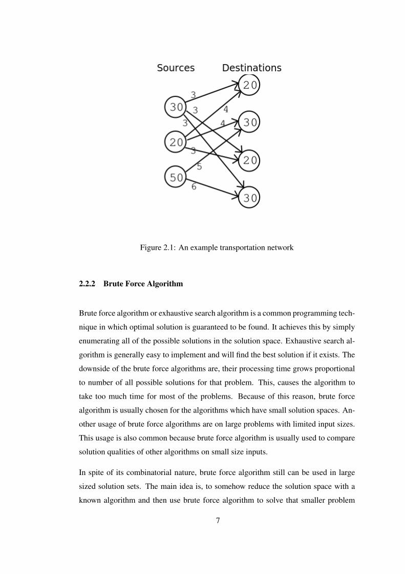
Figure 2.1: An example transportation network
2.2.2 Brute Force Algorithm
Brute force algorithm or exhaustive search algorithm is a common programming tech-
nique in which optimal solution is guaranteed to be found. It achieves this by simply
enumerating all of the possible solutions in the solution space. Exhaustive search al-
gorithm is generally easy to implement and will find the best solution if it exists. The
downside of the brute force algorithms are, their processing time grows proportional
to number of all possible solutions for that problem. This, causes the algorithm to
take too much time for most of the problems. Because of this reason, brute force
algorithm is usually chosen for the algorithms which have small solution spaces. An-
other usage of brute force algorithms are on large problems with limited input sizes.
This usage is also common because brute force algorithm is usually used to compare
solution qualities of other algorithms on small size inputs.
In spite of its combinatorial nature, brute force algorithm still can be used in large
sized solution sets. The main idea is, to somehow reduce the solution space with a
known algorithm and then use brute force algorithm to solve that smaller problem
7
instance. For example, if some of the solution space is known to be not optimal, that
part of the solution space may be eliminated by a preprocessing technique. After
preprocessing is made, the brute force algorithm will take less amount of time. Also,
another usage of brute force algorithms is to first reduce the size of the problem with
the help of a heuristic algorithm and then use a brute force algorithm to solve that
reduced problem.
2.2.3 Greedy Algorithm
Greedy algorithm is a type of heuristic algorithm which tries to find a solution by
choosing the best possible option at each decision point. The nature of the algorithm
is fast, because its processing time is not proportional to solution space. It usually can
not find optimal solutions for large sized inputs, because choosing the local optimal
solutions at each decision point does not guarantee to find the optimal solution.
Despite the disadvantages of optimality, greedy algorithm is still a widely used algo-
rithm technique. For the cases which has a very large solution space, finding optimal
solutions is not feasible. For this kind of situations, finding some correct solution in
a small amount of time is valuable. For this kind of combinatorial problems where
approaching exact algorithms is not possible, greedy based algorithms are commonly
used.
2.2.4 Linear Programming
Linear programming is a mathematical optimization method which tries to find best
possible outcome. The technique that linear programming uses is to represent the
problem as equations. With the help of bounding of the possible solutions and the
maximum and minimum possible values of the solutions, its objective function is
defined by a convex polyhedron. The solution space is the region involved by this
convex polyhedron. The optimal solution is the point where the objective function
takes its maximum or its minimum value.
Linear programming is a common method in operations research area. It can be used
8
to solve planning, production and transportation problems.
2.2.5 Mixed Integer Linear Programming
Integer programming is a special version of linear programming where all of the
solution variables are restricted to have integer values. In some of the problems, only
a specific part of the solution variables has the restriction of having integer values.
For this kind of cases, mixed integer linear programming is used. In most of the
scheduling problems, some values are restricted to have integer values. For example
the number of UAVs can not be a floating point number. For these kind of situations,
mixed integer linear programming method is used.
2.2.6 Branch and Bound Method
This is a paradigm to solve discrete and combinatorial problems. Its aim is, same
as the brute force algorithm. Both algorithms wants to find the optimal solution by
searching the solution space. Despite the similarities, branch and bound method is a
more robust method because it eliminates some parts of the solution space.
The idea of branch and bound method is to see the state space as a rooted tree and it
traverses the tree branches to find the optimal solution. Before going into a branch,
the algorithm checks the upper and lower estimated bounds to be an optimal solution.
If the branch can not provide a better solution than the current solution, then that
branch is eliminated from the state space.
This method is generally used for NP-Hard problems. While having better processing
times compared brute force algorithm, this algorithm is still too slow to be used in
real time problems.
2.2.7 Simplex Algorithm
Simplex algorithm is also a special type of linear programming algorithm. It also
makes use of linear equalities, linear inequalities and bounds. The difference of sim-
9

plex algorithm is that it works much faster than most of the linear programming al-
gorithms. The idea in the simplex algorithm is, to first look at the corners of the
polyhedron where the optimal solutions are most likely to be. With this way, it pro-
vides faster solutions than the most of the linear programming methods.
2.2.8 Matlab Intlinprog Utility
The main idea of this approach is, to divide the problems into multiple transporta-
tion problem instances and find an alternative solution to multiple constraint UAV
scheduling problem. Matlab is chosen for implementation because in Matlab there is
an optimization toolbox available which provides many tools to solve these kind of
planning problems.
Then, the appropriate function in Matlab optimization toolbox should be chosen. To
find the most suitable option to solve the problem with Matlab, the problem in hand
is analyzed at first.
The purpose in transportation problem is to minimize cost depending on all other
expressions as constraints. All the expressions including the objective function, are
linear in this problem. Matlab provides a table to choose the suitable function to use
for the problem. So, linprog is chosen Figure 2.2.
Though linprog seems really appropriate for the problem setting, it can not be used
for the solution. Because in the solution matrix it returns, there can be some non-
integer values. This function minimizes the objective function and finds the optimal
result but while making this, it assign non-integer values to solution variables. In this
problem, the cost is calculated as the summation of the products of the cost to go to
a particular target and the number of UAVs sent (the flow). So, finding number of
UAVs sent as a non-integer value is a wrong answer for this problem even thought it
is the optimal answer. This problem needs integer values for the solution variables.
There is a function available for achieving this condition. Name of this function is
intlinprog. It takes exactly same inputs with the linprog function. The only difference
is that it finds optimal result achievable with the integer values. So, intlinprog is used
to implement transportation function.
10
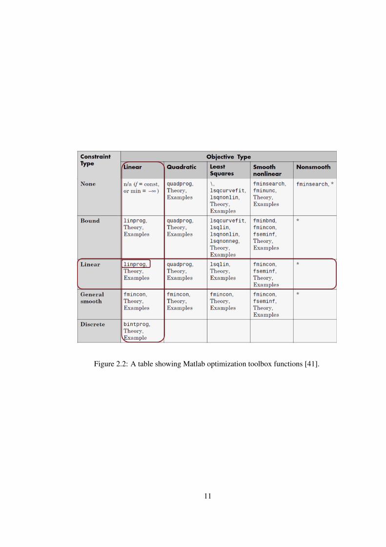
Figure 2.2: A table showing Matlab optimization toolbox functions [41].
11

The signature of the function used is as the following:
[x,fval]=intlinprog(f,intcon,A,b,Aeq,beq,lb,ub);
Intlinprog is an integer programming algorithm implementation. So, it only solves
the problems given in a specific form. That form is summarized below:
minxfTx (2.1)
A.x ≤ b, (2.2)
Aeq.x = beq (2.3)
lb ≤ x ≤ ub (2.4)
The Equation 2.1, shows the objective function of the linear programming problem.
The Equation 2.2, shows the linear inequalities, Equation 2.3 shows, the linear equal-
ities and finally Equation 2.4 shows, bounds of the linear programming problem.
12

CHAPTER 3
RELATED WORK
In the last 5 years the number of people using UAVs more than doubled the amount
of people using UAVs before. Similarly, the number of producers and developers
are also increased. This situation encouraged growing interest in the research involv-
ing UAVs. In the recent years, with the technological advances there is a dramatic
increase in the number of research made which make use of UAVs.
In this chapter we provide published work on UAV applications, different problem
types and solution methods in the literature.
3.1 UAV Applications
The UAV applications were used to be limited with only military applications before
but nowadays the situation has changed. Now, there is a wide variety of applications
on the civilian and military areas are produced every other day [52]. The rest of
the chapter provides examples of published works about military and non-military
applications.
3.1.1 Non-military Applications
Non-military applications including both civil and commercial applications are usu-
ally in the areas of; aerial mapping, oil and gas industry, broadcasting, disaster man-
aging, homeland security etc [6]. UAVs can easily make broadcasting from a place
where a man can not reach and also they can change place with the help of controller.
13
As an illustration to broadcasting usage of the UAVs some of TV channels started
to use UAVs in live TV coverage [1]. Not to mention, another usage of UAVs is for
monitoring critical places like oil pipelines to avoid unexpected hazardous situations
[42]. In the same fashion, another notable usage of UAVs in civilian applications
is on the disaster management topic. After natural disasters occurs there is a need
to gain information from the disaster area in a fast fashion. UAVs are suitable for
this job because they are small, they do not need any human controller in the dan-
gerous area and they are durable. S. M. Adams and C. J. Friedland at al. [2] and T.
Chou and M. Yeh and Y. Chen and Y. Chen at al. [12] studied disaster management
because of the above mentioned reasons. Environmental protection is an important
issue in the nowadays world. For protecting some habitats there is a need to monitor
them. Monitoring constantly is important for realizing changes and good for realizing
extraordinary urgent situations. Using an unmanned system, for example a flock of
UAVs, is suitable for this kind of a long and stable job. R. AI-Tahir and M. Arthur at
al. [3] studied on a system to make aerial mapping of a small area to both protect and
sense the changes in that environment.
3.1.2 Military Applications
Likewise non-military applications there are numerous military applications that make
use of UAVs. The current and possible future applications are explained in the study
of D. Glade at al. [28]. According to this study the applications that can use UAVs
are the followings; transportation, signals collection, intelligence, surveillance and
reconnaissance, combat support missions etc. Most of the military missions includes
collecting various kind of data and signals. Mini UAVs are hard to be recognized,
durable and fast. Because of these reasons mini UAVs are used for these kind of mis-
sions [13]. Surveillance missions are hard missions for most of the pilots because they
took long time and in the great majority of the missions the pilots have to wait. They
don’t have chance to use their hardly won skills. Because of these situations much
research is made on autonomous surveillance [25, 40]. Identically for the combat
support missions and reconnaissance mission using autonomous agents are preferred
[21].
14

3.2 Problem Types
In this part we provide problem variations related to our problem. The problem
studied in this thesis is a multiple-constraint UAV scheduling and target assignment
problem and it is also a special version of surveillance and reconnaissance mission.
Surveillance and reconnaissance missions are usually complex problems that most of
the problem instances can not be solved by using a single UAV. Instead of that, co-
operation of UAVs is needed to achieve some certain needs of that specific problem
[11]. Because of this reason, most of the studies in the literature is on cooperation.
However, another notable thing about this research area is the variability of the prob-
lem instances. There are numerous different problem instances and for each of them
the needs of the problem changes in a different manner. This yields many different
solutions for many different problems [24].
For mission planning problems, the major reason of the variability is the nature of
constraints. Each different problem has a different nature; so, this causes that each dif-
ferent problem has different constraints. There are roughly two types of constraints.
The ones used in the applications which try to simulate a realistic model in terms
of the UAV aerodynamics which takes real time constraints into account. The second
type of constraints are focusing on scheduling and target assignment. They have some
simple assumptions for the aerodynamics of the UAVs but they focus on solving more
complex assignment and scheduling problems.
To demonstrate one of the frequently used constraints in realistic models is minimum
segment length [17, 7, 37, 53]. This constraint is about the behavior of the UAVs.
A UAV must not change any attitude in the flight before traveling to some predeter-
mined distance when this constraint is present. This constraint is generally used in
simulations which is used to make a more realistic design. By this constraint an UAV
can complete one turn before starting another. Next example constraint is maximum
turn angle constraint. This constraint is also associated with the limits of the real life
UAVs. UAVs can make turns with some limited angles. The problems having this
constraint takes maximum turn angle limit into consideration while finding solutions
[33, 32]. Furthermore, another constraint is minimum flight altitude constraint. This
constraint can be seen in 3D simulations mostly. All of the aerial vehicles should fly
15

above a minimum flight altitude [57, 29, 16]. UAVs in real life can not dive or climb
with very steep angles like 90 degrees this type of behavior can cause the UAV to fall
down. Hence, maximum climbing angle or maximum diving angle are limited. This
constraint is again for 3D simulations [58, 60].
The first example of constraints that are frequently used in target assignment and
scheduling problems is the capacity constraint. This constraint is generally used in
vehicle routing problem VRPs. In these kind of problems every vehicle has a con-
stant capacity and can not serve more than that amount [19, 56, 9]. Moreover another
different problem instance is the one with heterogeneous UAVs. In this problem in-
stance, UAVs can have different velocities and fuel capacities in the beginning on
the scenario. So, choosing the best suitable UAV for the mission is also an another
important issue [35, 22]. Vehicle routing problem with time windows is another prob-
lem instance in which targets can only be visited in some predetermined time periods
[15, 10, 38]. Next constraint is stochastic one. Here one or more of the components
of the problem are random. For example, sources, demands or time windows can be
stochastic [43]. Fuel constrained systems is one of the popular problem instances. In
this problem instance UAVs have limited fuels. So, while assigning UAVs to targets
one should control if the fuel to go from current place of the UAV and go back to base
station of the UAV is enough [27].
3.3 Solution Methods
There are numerous problem instances and solution methods for UAV mission plan-
ning problems. Solution methods can be classified into two main clusters: Centralized
methods and decentralized methods. In centralized methods there should be a control
system and there should be agents. First, the control system gathers agent status in-
formation and environmental information. Then, it runs the algorithm and finds the
flight plan, UAV target assignments and their velocities. After that the control system
passes information to UAVs and the UAVs do their job [5, 47]. In decentralized meth-
ods, the mechanism is a little different. First of all, there is no control system in the
decentralized method. The idea is to divide the main problem into many small prob-
lem instances and solve them one by one [36, 31, 45]. While doing this, the biggest
16

problem is with the coordination of the UAVs because there is no control system that
is telling what to do. Each UAV should analyze its status, communicate with the other
UAVs and then decide what to do. The advantage of the decentralized approaches is
that each sub problem requires a small search space. However for big search spaces
and complex problems centralized approaches seem to be more feasible. In the fol-
lowing chapters we provide example studies that uses decentralized and centralized
methods.
3.3.1 Decentralized Methods
The first example of the decentralized model is the strategy of having a single leader
for the flock and the others follows it [20, 49]. The idea of this method is selecting
a leader and position other UAVs according to it. With this way it is possible to find
exact places of the whole flock just by finding the place of the leader. Although this
looks a good and clear strategy to approach, if the leader fails this strategy loses its
effectiveness. Furthermore, the communication between the flock members is not ef-
fective in this application. The second example of the decentralized model is virtual
structure method. In this method, the whole flock behaves like a single entity [39].
Next, there is a key concept about decentralized model; it is behavior based method.
In this method, the team goes within a formation but with the environmental changes
they need to adopt to the changing environments. They change formation in order
to adopt to environment. Behavior based model is inspired from animal flocks. For
example, bird flocks change formation when they are passing through a narrow place.
They can even go one by one if the passageway is too narrow. After the environment
is big enough they return to starting formation. In behavior based method this types of
behavior is aimed. They preserve this formation by communicating with each other
[55, 54]. Another method is to changing planning space into the field space. This way,
all the obstacles and the places that UAVs should not go are surrounded by repulsion
forces and the goal is surrounded by forces of attraction. The collision avoidance
and reaching goal by agents are achieved by this method. The method is called ar-
tificial potential field method [23, 14]. One of the key decentralized approaches is
graph theory based method. In this model a graph containing UAV information and
communication links are created. The nodes correspond to UAVs and edges corre-
17
sponds to relationships between the UAVs. With the help of this graph UAV control
is achieved. Furthermore, addition of new nodes and deletion of existing nodes are
easy to control [44].
3.3.2 Centralized Methods
For the centralized methods a control system exists in the environment. Control sys-
tem runs the offline algorithm and transmits this information to the UAVs. There
are two main cluster of algorithms for the solutions. These clusters are exact algo-
rithms and heuristics. In exact algorithms, the main idea is to find the best solution by
searching the whole solution space. Although searching the whole solution space is
too slow for even the easy problems, with some elimination from the solution space,
algorithms can find faster solutions. The elimination process is usually done before
starting the search. These eliminations are usually made on solutions that seem obvi-
ously wrong. The variation on exact problems are usually caused by the differences
in elimination techniques. Exact algorithms usually find optimal solution but despite
the eliminations they are still too slow for large and complex problems. Because of
this reason, there are many heuristic approaches in the area. The idea behind the
heuristic approaches is finding an acceptable solution in a fast way. They may not
find optimal solution for all of the problem instances but they are fast and if finding
the optimal solution is not a must and finding an acceptable true solution is enough
then using heuristics is a good idea. Heuristics usually search a small but effective
part of the solution space. Because of that they find local optimal solutions but in a
fast way [46].
Integer programming is a good example of the exact algorithms for the UAV mission
planing problems. The problem is encoded into a mathematical model. The con-
straints are converted into mathematical equalities and inequalities. Then, an objec-
tive function is created. With the help of these equalities and inequalities, the optimal
values are found with the help of matrix operations. For example, Bellingham at al.
[8] worked on control and coordination of UAV flocks with Mixed Integer Linear
Programming (MILP). Some of the variables are integers where some others are not.
The mixed term comes from the mixture of the integer and floating point values in
18

the solution variables. Similarly, Schouwenaars, Moor, Feron and How worked UAV
mission planning using MILP [48]. Another notable exact algorithm is dynamic pro-
gramming. In dynamic programming the aim is to break up the problem into smaller
instances and solve them. Then, combine the solutions of the smaller problems to
reach the optimal solution. Alighanbari and How at al. [4] worked on a cooperative
target assignment problem in adversarial environments with dynamic programming.
UAV mission planning algorithms usually have a complex nature. So, exact ap-
proaches are infeasible in terms of running times for most of the cases. For this
reason, heuristic approaches are more popular. For the heuristic paradigm, there are
three types of algorithms. Probabilistic algorithms, genetic algorithms and heuristic
algorithms. In probabilistic approaches, the agents make choices randomly to take to
the next step. Although probabilistic approaches are not very effective they provide
searching through the different areas of the solution space. They are usually used in
hybrid approaches [18]. The genetic algorithms or evolutionary algorithms are one of
the most popular heuristic methods [26, 50, 30, 51, 34]. Heuristic algorithms are in
the same direction with the genetic algorithms. In a certain way, they create a small
subset of the solution space and they find the solution using that small subset. The
subset is not randomly chosen. They usually build these subsets by making guesses
using the domain information that is available to them. One example of heuristic al-
gorithm is greedy algorithm. As the name implies greedy algorithm chooses the best
possible option at each decision point. Although this seems like a good idea to reach
the optimal solution sometimes the algorithm should not choose the best possible op-
tion. The real importance of greedy algorithms is that they are fast. Because, they
search only a small part of the solution space [59].
19

20
CHAPTER 4
PROPOSED WORK
This chapter provides a detailed description of our study of multiple constraint UAV
scheduling and target assignment problem. First, the problem structure is defined.
Then, the constraints of the problem in hand are defined. After that, the environmental
assumptions are given. Then, a brief explanation about how inputs are generated will
be made. Lastly, proposed algorithms are presented.
4.1 Problem Description
UAV mission planning is a type of target assignment and UAV scheduling problem.
UAV mission planning problem is defined as determining assignment and scheduling
of UAVs to targets that minimizes the total cost. First of all, there are some UAVs
and targets in this problem. At the beginning of the problem UAVs start from a base
station. Then, each of the targets should be visited by some required number of
UAVs. All UAVs must return back to the base station, after the traversal. Figure 4.1
contains an example. This example shows a snapshot from a UAV mission planning
scenario. In the example, rectangle represents base station and circles represents
targets. Arcs connecting the rectangle and the circles represent costs to reach from
one of the connected nodes to another. For this example, there is no environment
constraints. Environment of the problem defines the physical rules that taken into
consideration while solving the problem. When there is no environment constraint,
UAVs can use euclidean distance path to go from one target to another. All UAVs
and targets have unique ids to distinguish from each other. Again in the figure all the
21

targets has something like tw=[1-5]. Tw stands for time window. Targets are only
available in these time intervals and they have to be visited at the beginning of the
time windows. Furthermore, once a UAV reached a target it can not leave it before
departure time of that target. So, if two target’s time windows are overlapping, the
same UAV can not visit both of them. Some targets have larger areas to be covered
than others. So, sometimes one UAV can not finish the mission at that target itself.
For this kind of situations, number of UAVs needed must be defined. If a target need
is 2, then that target must be traveled by two UAVs and these UAVs can not be the
same UAV. Simulation time that is placed in the top left corner shows the time of the
mission. Time windows are activated according to that time value.
Figure 4.1: A sample drawing of the studied problem
In Figure 4.2, a base station holding 5 UAVs is provided. As can be seen from the
figure, each UAV has its own ids and apart from ids, all of the UAVs are identical.
Note that, UAVs are homogeneous. When the mission is completed, the current co-
ordinates and the base station coordinates of the UAVs must be the same. Each UAV
has a fuel constraint. To be able to achieve a mission, UAVs should have enough fuel
in their tanks to return back their own base stations.
The objective is to minimize the cost of traversal of all targets. The total cost is
calculated by the summation of the total consumed fuels by all UAVs.
22
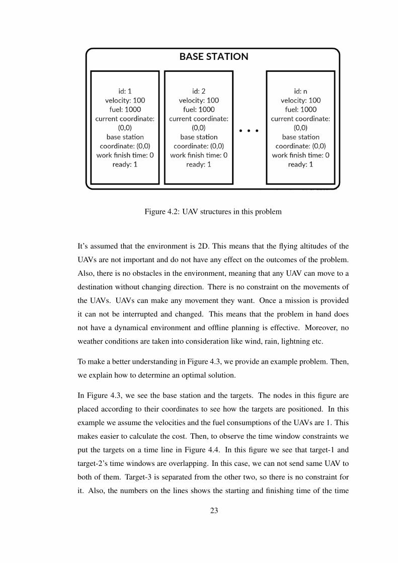
Figure 4.2: UAV structures in this problem
It’s assumed that the environment is 2D. This means that the flying altitudes of the
UAVs are not important and do not have any effect on the outcomes of the problem.
Also, there is no obstacles in the environment, meaning that any UAV can move to a
destination without changing direction. There is no constraint on the movements of
the UAVs. UAVs can make any movement they want. Once a mission is provided
it can not be interrupted and changed. This means that the problem in hand does
not have a dynamical environment and offline planning is effective. Moreover, no
weather conditions are taken into consideration like wind, rain, lightning etc.
To make a better understanding in Figure 4.3, we provide an example problem. Then,
we explain how to determine an optimal solution.
In Figure 4.3, we see the base station and the targets. The nodes in this figure are
placed according to their coordinates to see how the targets are positioned. In this
example we assume the velocities and the fuel consumptions of the UAVs are 1. This
makes easier to calculate the cost. Then, to observe the time window constraints we
put the targets on a time line in Figure 4.4. In this figure we see that target-1 and
target-2’s time windows are overlapping. In this case, we can not send same UAV to
both of them. Target-3 is separated from the other two, so there is no constraint for
it. Also, the numbers on the lines shows the starting and finishing time of the time
23

Figure 4.3: An example problem setting, targets are placed according to their coordi-nates.
windows.
Figure 4.4: An example problem setting, targets are placed according to their timewindows.
To be able to decide which choice is the best, we created a cost table that shows the
cost to reach from one target to another. In Table 4.1, 0 represents the base station
and the other numbers represent the ids of the targets.
The optimal solution for this problem instance is provided at Table 4.2. Targets and
assigned UAVs are provided with their costs. While deciding this solution, things to
24

Table 4.1: Table shows costs to reach from a target to another.
Cost Matrix0 1 2 3
0 0 3,61 4,24 14,211 3,61 0 1 10,632 4,24 1 0 103 14,21 10,63 10 0
consider are the constraints. The first of the current constraints is not sending the
same UAV to both target-1 and target-2. The second one is to minimize the fuel.
Table 4.2 represents the best possible solution for this problem. On the other hand,
in Table 4.3, we provide another possible solution. The difference between these two
solutions is, in solution-2 a new UAV is send from the base station. On the contrary,
solution-1 sends the UAV which is closer to target-3. With this way it minimizes the
fuel consumption
Table 4.2: Optimal solution for this problem is presented in this table.
Solution 1- Total Cost : 17,85Target Id Uav Id CostTarget 1 UAV 1 3,61Target 2 UAV 2 4,24Target 3 UAV 2 10
Table 4.3: Another possible solution to solve this problem.
Solution 1- Total Cost : 22,06Target Id Uav Id CostTarget 1 UAV 1 3,61Target 2 UAV 2 4,24Target 3 UAV 3 14,21
4.2 Proposed Solution Methods
In this part, algorithms developed to solve UAV mission planning problem are de-
scribed. There are five algorithms proposed in the scope of this thesis. The two of
them are developed to test the proposed algorithms in terms of solution quality and
performance. The other three of them are approaches with similar infrastructures.
25
They are developed in order to solve multiple constraint UAV mission planning prob-
lem and assess their performances.
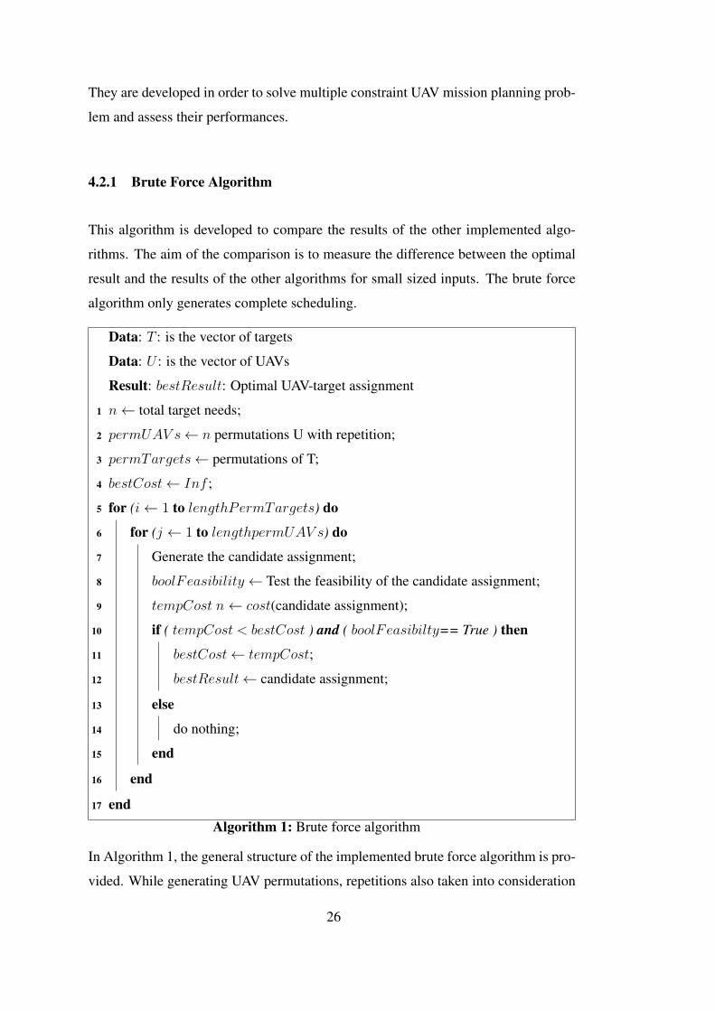
4.2.1 Brute Force Algorithm
This algorithm is developed to compare the results of the other implemented algo-
rithms. The aim of the comparison is to measure the difference between the optimal
result and the results of the other algorithms for small sized inputs. The brute force
algorithm only generates complete scheduling.
Data: T : is the vector of targets
Data: U : is the vector of UAVs
Result: bestResult: Optimal UAV-target assignment
1 n← total target needs;
2 permUAV s← n permutations U with repetition;
3 permTargets← permutations of T;
4 bestCost← Inf ;
5 for (i← 1 to lengthPermTargets) do
6 for (j ← 1 to lengthpermUAV s) do
7 Generate the candidate assignment;
8 boolFeasibility← Test the feasibility of the candidate assignment;
9 tempCost n← cost(candidate assignment);
10 if ( tempCost < bestCost ) and ( boolFeasibilty== True ) then
11 bestCost← tempCost;
12 bestResult← candidate assignment;
13 else
14 do nothing;
15 end
16 end
17 endAlgorithm 1: Brute force algorithm
In Algorithm 1, the general structure of the implemented brute force algorithm is pro-
vided. While generating UAV permutations, repetitions also taken into consideration
26
because the same UAV can go more than one target. For target permutations, we only
generated permutations without repetition. By creating these two sets, we are able
to search whole solution space. A pre-elimination procedure can be added to this
implementation in order to increase the efficiency of this algorithm.
4.2.2 Greedy Algorithm
This algorithm is also developed to compare the results of the other algorithms to
assess test the solution qualities and time consumptions. The greedy algorithm has a
faster nature than brute force algorithms. Actually it is one of the fastest approaches
to a problem. So, this provides a lower limit on the elapsed time constraint. If an
algorithm displays a performance that has a similar speed then that algorithm can
be counted as a really effective algorithm. Constructing an algorithm which has a
similar speed as greedy algorithm, cost values smaller than greedy algorithm and
solution finding ratio larger than greedy algorithm is a really valuable achievement
for this problem. To be able to make these kinds of experiments greedy algorithm is
27

also implemented.
Data: T : is the vector of targets
Data: U : is the vector of UAVs
Result: Result: Found UAV-target assignment
1 sortedTargets← sort(T ) /* sort targets according to their
time windows, in increasing order */
2 while (isEmpty(sortedTargets)==False) do
3 chosenTar← chooseTarget(sortedTargets);
4 U ← updateUAV status(currentT ime);
5 if anyReadyUAV s(U )==True then
6 chosenUAV ← chooseLeastCostUAV (chosenTar, U);
7 (U, sortedTargets)← sendUAV toTarget(chosenUAV ,chosenTar)
/* update UAVs and targets */
8 Result← Result + (chosenUAV ,chosenTar)
9 else
10 currentT ime← updateT ime();
11 end
12 endAlgorithm 2: Greedy Algorithm
Algorithm 2 shows the steps of greedy the algorithm.The main idea of the greedy
algorithm is, to send UAVs to targets with the minimum cost as long as there are
UAVs ready. If all the UAVs are on a mission, current time is updated to the time
when first UAV will finish its work. Traversing order of targets are defined with their
time windows in this algorithm. If start of
4.2.3 Divide and Conquer Algorithm
The idea to solve multiple constraint UAV scheduling and target assignment prob-
lem is to divide the problem into smaller problem instances and solve the smaller
instances. Then, combine the results. As can be seen in Figure 4.5, converting UAV
mission planning into multiple transportation algorithms is the key point of our pro-
posal. Hybrid greedy algorithm, intlinprog heuristic algorithm and simplex heuristic
28

algorithm uses this divide and conquer idea. The only difference is each of them
solves the sub problems with a different algorithm. Actually they take their names
from the approaches they attack to solve transportation problem. Apart from that in-
frastructures of all of these three algorithms are the same. They are implemented in
order to see which one of them suits best for the problem.
Figure 4.5: UAV structures in this problem
The idea behind our proposal is to cluster the targets according to their time window
values. Then from the beginning of the each cluster solve the transportation algorithm
and then combine all the results. This algorithm is actually a special version of greedy
algorithm but it should have find much more effective results than greedy algorithm
because the amount of search space scanned is much more than the greedy algorithm.
It is important to realize that when all of the targets are individual clusters this idea
works as in the exactly same way with the greedy algorithm but this is only one
29
extreme case.
Data: T : is the vector of targets
Result: Clusters: is the vector of clustered targets
1 sortedTargets← sort(T ) /* sort targets according to their
time windows, in increasing order */
2 while (isEmpty(sortedTargets)==False) do
3 chosenTar← chooseTarget(sortedTargets) /* choose target
with smallest time window start */
4 newClusterF lag← True;
5 for (j ← 1 to lengthClusters) do
6 if overlapWithCurrentCluster(chosenTar)>0.7 then
7 currentCluster← currentCluster + chosenTar;
8 newClusterF lag← False;
9 break;
10 else
11 do nothing;
12 end
13 end
14 if newClusterF lag == True then
15 currentCluster← newCluster;
16 newCluster← chosenTar;
17 Clusters← Clusters + newCluster;
18 else
19 do nothing;
20 end
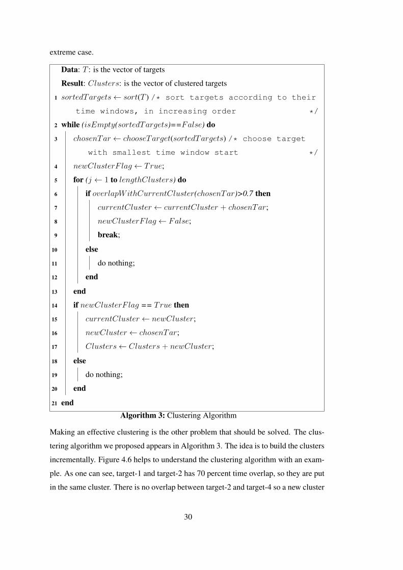
21 endAlgorithm 3: Clustering Algorithm
Making an effective clustering is the other problem that should be solved. The clus-
tering algorithm we proposed appears in Algorithm 3. The idea is to build the clusters
incrementally. Figure 4.6 helps to understand the clustering algorithm with an exam-
ple. As one can see, target-1 and target-2 has 70 percent time overlap, so they are put
in the same cluster. There is no overlap between target-2 and target-4 so a new cluster
30
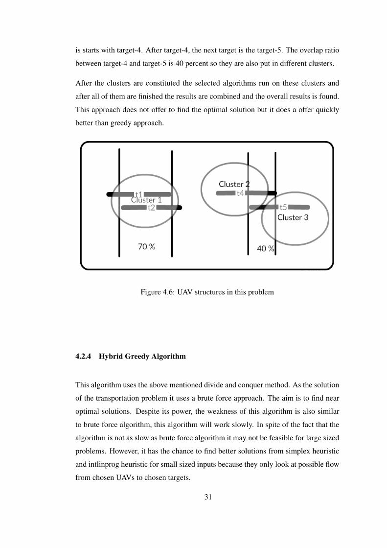
is starts with target-4. After target-4, the next target is the target-5. The overlap ratio
between target-4 and target-5 is 40 percent so they are also put in different clusters.
After the clusters are constituted the selected algorithms run on these clusters and
after all of them are finished the results are combined and the overall results is found.
This approach does not offer to find the optimal solution but it does a offer quickly
better than greedy approach.
Figure 4.6: UAV structures in this problem
4.2.4 Hybrid Greedy Algorithm
This algorithm uses the above mentioned divide and conquer method. As the solution
of the transportation problem it uses a brute force approach. The aim is to find near
optimal solutions. Despite its power, the weakness of this algorithm is also similar
to brute force algorithm, this algorithm will work slowly. In spite of the fact that the
algorithm is not as slow as brute force algorithm it may not be feasible for large sized
problems. However, it has the chance to find better solutions from simplex heuristic
and intlinprog heuristic for small sized inputs because they only look at possible flow
from chosen UAVs to chosen targets.
31

4.2.5 Intlinprog Heuristic Algorithm
This algorithm also uses the above mentioned divide and conquer method. After the
clusters are constituted, this algorithm solves transportation problem with a modified
linear programming algorithm. To implement this algorithm, the Matlab optimiza-
tion toolbox’s intlinprog function is used. The data is prepared to be suitable for
intlinprogs parameters. Then intlinprog is run for each of the transportation problem
instances. At the end the found solutions are combined. In Algorithm 4, the steps
of Matlab’s intlinprog algorithm is presented. Mix integer linear programming and
branch and bound algorithms are explained in the background section.
Data: T : is the vector of targets
Data: U : is the vector of UAVs
Result: Result: Found UAV-target assignment
1 it reduces the problem size by applying some linear programming
preprocessing;
2 solves the initial problem with the help of linear programming;
3 performs mixed integer linear programming and cut generation to tighten the
LP relaxation;
4 uses branch and bound algorithm to reach the optimal solutions;
Algorithm 4: Intlinprog Algorithm
In the following parts we explain how we constructed the equations and the objec-
tive function to use linear programming. Also, we explain the usage of intlinprog
algorithm to solve UAV mission planning problem.
4.2.5.1 Construction of the Linear Programming Equations
In this part the problem is converted into a mathematical model. For linear program-
ming problems linear equalities, linear inequalities, bounds for the solution variables
and an objective function need to be generated.
To construct linear equalities, constraints of the problem need to be extracted. There
are two constraints available for this problem:
32

1. Only some of the UAVs are available for each sub-problem. And each UAV
can only visit one target at a time. Because of this, for each of the source, the
number of items it can send to destination is fixed.
2. For each target, the number of UAVs it needs is fixed.
According to these constraints, the equations are constructed. It is assumed that, the
number of sources available is n and the number of destinations available is m. For
each source and destination, there is exactly one constraint. So, there can be n + m
equations for this problem.
For each of the sources, the number of UAVs it have is shown as: S1,S2,S3 ... Sn . This
shows how many UAVs that each of the source can send. For each of the destinations,
the number of the UAVs they can receive is shown as: D1,D2,D3 ... Dm .
Number of UAVs sent from each source to destination is hold in a matrix. This matrix
is used to construct the equations. In Table 4.4, we see an example of this matrix. In
the matrix, number of UAVs sent from S1 to D1 is showed with u11 and UAVs sent
from S2 to D2 is showed with u22 and so on.
Table 4.4: A matrix showing UAVs send from a source to a destination
d1 d2 d3 ... dm
s1 u11 u12 u13 u1m
s2 u21 u22 u23 u2m
s3 u31 u32 u33 u3m
...sn un1 un2 un3 unm
With the help of the matrix and the above mentioned constraints, the following (n+m)
number of linear programming equations are constructed:
m∑i=1
u1i = S1 (4.1)
33

m∑i=1
u2i = S2 (4.2)
m∑i=1
u3i = S3 (4.3)
m∑i=1
uni = Sn (4.4)
n∑i=1
ui1 = D1 (4.5)
n∑i=1
ui2 = D2 (4.6)
n∑i=1
ui3 = D3 (4.7)
n∑i=1
uim = Dm (4.8)
For this problem no inequalities exist. Also, no upper bounds exist for the number
of UAVs sent. So, upper bounds can be chosen as infinite. It is not possible to send
negative number of UAVs to a target. So, lower bound for the solution variables is 0.
The objective function of the problem defines the value that needs to be minimized. In
this problem value to be minimized is the total cost. The total cost is the accumulated
sum the fuels consumed by all of the UAVs. Let’s call the total cost C. Equation 4.9
shows the way C is calculated:
C = Σmi=1(Σ
kj=1cij) (4.9)
cij is the cost of going from the current location of the UAVj to the targetis location.
The m in the formula is the number of targets and the k in the formula represents the
number of UAVs at each of the targets.
34

4.2.5.2 Usage of Intlinprog Algorithm
In this part usage of Matlab’s intlinprog function is explained. The signature of the
function used is as the following:
[x,fval]=intlinprog(f,intcon,A,b,Aeq,beq,lb,ub)
As the Matlab suggets x and fval are the outputs of the function. f, intcon, A, b, Aeq,
beq, lb and ub are the input parameters of the function. In intlinprog, the inputs repre-
sent the various constraint types of the problem and the outputs represents the results.
Intlinprog takes input in the following order: first linear inequalities then linear equal-
ities and finally bounds. According to this, A is the matrix of linear inequalities and
b is a vector holding the right hand side values of the inequalities. Similarly, Aeq and
beq are used for equalities. lb is the vector holding lower bound values and ub is the
vector holding upper bound values.
4.2.6 Simplex Heuristic Algorithm
In this chapter proposed work of this thesis is explained. The idea is to divide schedul-
ing and assignment parts of the problem. Solve each assignment problem individually
and combine the results. In this idea, there are two important parts: The first one of
them is how to divide this problem. The solution of this part is explained in divide
and conquer algorithm section. The second part of this idea is how to construct a
transportation problem.
The divided problem has time window constraints and scheduling of the UAVs is
needed. On the other hand, transportation problem finds a transportation plan but it
does not do scheduling. It only makes an assignment between sources and destina-
tions. It does not do anything related to time. Meaning that, the solutions it produces
does not indicate the orders of the assignments. Furthermore, the solutions it produces
are optimal solutions.
In the rest of the section, we provide a design to transform the sub-problems into
transportation problem. Then, a brief explanation about why simplex algorithm is
chosen to solve the generated transportation problem is given. Finally, a pseudo code
35

explaining the working structure of the primal simplex network algorithm is provided.
4.2.6.1 Problem Design
In this part design to transform sub-problems into transportation problems are ex-
plained. The steps of this process is explained in Algorithm 5.
Data: U : is the vector of UAVs
Data: T : is the vector of targets
Data: currentT ime: is the vector of targets
Result: Sources: source vector of the transportation problem
Result: Destination: destination vector of the transportation problem
1 AvaibleTargets← findAvaibleTargets(targets,currentT ime)
2 for i← 1 to lengthUAV s) do
3 for (j ← 1 to lengthAvaibleTargets) do
4 if (reachT ime(UAV s[i]) < target[i].timeWindowStart) then
5 avaibleUAV s← avaibleUAV s + UAV s[i] ;
6 break;
7 else
8 do nothing;
9 end
10 end
11 end
12 Sources← ClusterSameCoordinateUavs(avaibleUAvs);
13 Destinations← avaibleTargets ;
14 solveTransportationAlgorithm(Sources,Destinations);
Algorithm 5: Transportation algorithm design
To explain the algorithm better, an example is prepared. In this example, we examine
a mission planning problem. With the help of diving procedure explained above we
find first sub-problem. Then, convert it to a transportation problem. In Figure 4.7, a
snapshot from a simulation is provided. In this example, at the current time instance
there are 10 UAVs in the base station and 5 UAVs are in the targets. The works of the
UAVs with ids 1, 2 and 3 are finished at 9th second and the works of the UAVs with
36

ids 4 and 5 finishes at 13th second.
Figure 4.7: An example snapshot from UAV Mission Planning Problem
The next cluster to be visited can be seen in Figure 4.8. In this figure we see three
targets to cover. To eliminate scheduling, we determine the ready UAVs. Then, from
this set we make an elimination. For each UAV, we calculate the possible reaching
times to targets. If reaching time is smaller than or equal to starting time of the target,
then that UAV is marked as available. After the eliminations made, the next step is to
cluster UAVs according to their coordinates. For this example, there are three clusters
of UAVs; base station, the UAVs at target 1 and the UAVs at target 2. Each of these
places are taken as sources. Also, the targets are the destinations. Needs of each
target is, taken as the capacity on that destination.
In Figure 4.9, the resulting transportation problem is provided. The left circles repre-
sent the sources and the right circles represent the destinations. The capacity of each
source and destination is written into the center of the circles. The capacities of the
sources are 10, 3 and 2 respectively. Because, at base station there are 10 UAVs, at
target-1 there are 2 UAVs and at target-2 there are 3 UAVs. After this point, the prob-
lem is converted into a transportation problem. The solution of transportation problem
yields a minimum cost flow. For our case, results show optimal UAV-target assign-
ments. In Figure 4.9, arcs between sources to destinations shows how many UAVs
37

Figure 4.8: An example snapshot from UAV Mission Planning Problem
are send from each source to destination. After solving the transportation problem,
we add cost of each UAV to the current time value and calculate the times that UAVs
are assigned to targets. With this way time information is added to this design.
Each assignment found from the sub-problems, are placed into a table holding the re-
sults. After solving all of the sub-problem a scheduling and assignment table showing
the results is produced. An example solution table can be seen in Table 4.5.
Table 4.5: An example table showing the result of an UAV mission planning
Assignments Target Ids Uav Ids Assigned Time Consumed Fuel1 1 1 0,8 152 1 2 4,30 453 1 7 6,35 644 2 1 6,45 105 3 4 8,32 22,56 3 5 10 38
4.2.6.2 Primal Network Simplex Algorithm
For primal simplex algorithm, we used an implemented algorithm provided at Matlab
file exchange. It takes a capacity matrix, source matrix and a cost matrix. It returns
38
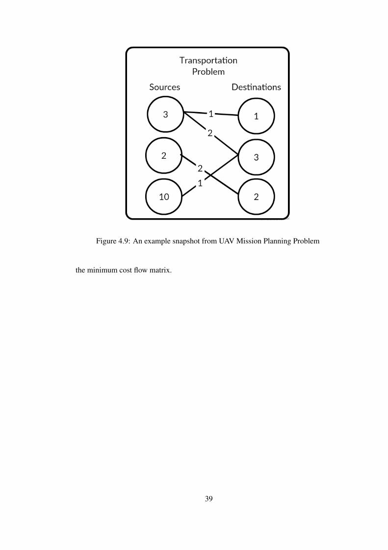
Figure 4.9: An example snapshot from UAV Mission Planning Problem
the minimum cost flow matrix.
39

40
CHAPTER 5
EVALUATION AND RESULT
In this chapter, performance evaluation of the proposed algorithms presented. We
show that simplex heuristic method fits better to this problem compared to the other
algorithms. The algorithms are evaluated on their effectiveness and their solution
qualities. We created a testing environment. The first thing we do was to examine the
effect of the size of the problem on the performance of algorithms. Also, similar prob-
lems are grouped together and all the algorithms are tested with characterized input.
The aim of doing this is to reveal the vulnerabilities or strengths of the algorithms.
5.1 Test Environment
First of all, Matlab provides a wide range of algorithms readily programmed. Matlab
has an optimization toolbox and this toolbox offers a wide range of algorithms to use.
This toolbox, comes already installed with the new versions of the Matlab. Further-
more, the structure of the problem is suitable for object based programming. It is also
possible to make object oriented programming with Matlab. Also, the transportation
algorithm requires a matrix based approach and Matlab fits in all of these necessities
nicely. Because of these reasons, Matlab is chosen as the programming language for
this study.
The version of the Matlab used in the experiments is Matlab R2014b. The project is
developed on a PC which has a 64 bit 3.40 GHz Intel i7 processor. The operating
system is Ubuntu 14.04.2 LTS operating system.
41

5.2 Data Sets
Three different input sets are prepared to evaluate the algorithms. All of the algo-
rithms are run on these sets and the solutions are compared. While making compari-
son average results of the algorithms are used.
The first input set contains problem instances of different sizes. The aim here is to
test the effect of problem size on the performances of the algorithms. Data sets inputs
are classified in three different clusters; small sized, medium sized and large sized.
Small input set contains 3 to 5 targets, medium ones have 7 to 10 targets and large
inputs have 20 to 25 targets. For each input type, 10 different inputs are created.
The second input set clusters the input in terms of time window values of targets. The
overlap rate of target time windows are calculated for each of the inputs. The inputs
are clustered according to their overlap rates. The aim is to observe the behaviors of
the algorithms on various overlap rates. Clustered inputs are created for different size
of inputs. Each cluster has 10 inputs cases.
The last input set is used to test the algorithms with handcrafted and randomly created
inputs. The aim of creating hand crafted inputs is to test some extreme cases. Fur-
thermore, it is possible to provide problem sets that are guaranteed to have complete
scheduling solutions with manual input creation. Unfortunately, randomly generated
inputs can not give this guarantee. On the other hand, random input generation is
needed to increase the variability of the inputs. All small sized, medium sized and
large sized inputs are created for both handcrafted input and randomly created input.
For each different sizes, an input set having 10 inputs are generated.
We developed a function to create randomly generated inputs. The function takes ratio
of overlaps, maximum and minimum time windows values and the coordinate ranges
as parameters. Then it generates random inputs satisfying these constraints. Note that
for randomly generated inputs, it is not possible to assess whether the created mission
can be solved fully or partially.
In the following sub-sections we provide explanations about overlapping ratio.
42

5.2.1 Overlapping Ratio
Overlapping ratio is calculated by the rate of overlaps in the target set. To calculate
this ratio, definition of overlapping must be done clearly. In this problem overlap is
the case when two targets time windows cover the same time interval. These time
intervals do not have to overlap completely, only a small overlap is an enough reason
to send two different UAVs to these targets because the UAV must stay at that target
until its time window finishes.
Figure 5.1, shows two different problem structures. For both of the problems the
overlapping ratio is same, it is 2/3. Overlapping ratio is calculated by dividing the
number of targets that overlap to the total number of targets. For this example, target-
1 and target-2 are overlapping. So, there are two overlapping targets and the total
number of targets is 3. Because of that, the ratio is 2/3. For the second example, first
two targets are totally overlapping but this does not change the ratio.
Figure 5.1: Two cases where overlapping ratio is same.
5.3 Input Generation
Two types of input are generated. We generated some test cases manually. The second
type of input is generated automatically and the inputs are randomized.
For random input the user can specify the number of targets, number of UAVs, max-
imum and minimum coordinates of targets, maximum and minimum time window
43

values and the ratio of overlaps. In Algorithm 6, the steps of random input generation
44

is provided.
Data: T : is the vector of targets
Data: U : is the vector of UAVs
Data: OR: expected overlapping ratio
Data: CI: coordinate interval
Data: V : velocity
Data: F : fuel
Data: UN : UAV numbers needed
Data: NU : number of UAVs
Data: NT : number of targets
Result: UAV s: A randomly created UAV vector
Result: Targets: A randomly created Target vector
1 for i← 1 to NU do
2 randomCoordinate← rand(CI);
3 UAV s← createRandomUAV s(i,F ,V ,randomCoordinates);
4 end
5 for i← 1 to NT do
6 if overlapRatio(U )<OR then
7 randomCoordinate← rand(CI);
8 lenClusters← length(Clusters);
9 selectedCluster← randi(0,lenClusters);
10 tempTarget← createRandomTarget(i,randomCoordinates,UN );
11 Targets← tempTarget;
12 Clusters← addToCluster(selectedCluster,tempTarget);
13 overlapRatio← updateOverlapRatio(Targets);
14 else
15 tempTarget←createRandomNonOverlappingTarget(i,Clusters,UN );
16 overlapRatio← updateOverlapRatio(Targets);
17 end
18 endAlgorithm 6: Random Input Generation
45

This random input generator makes it very easy to test the algorithms. Furthermore
with the help of overlap ratio parameter, inputs with different characteristics can be
created. In Figure 5.2, an example explaining the algorithm is provided. At first
situation two targets are already generated and current overlap rate is smaller than the
expected overlap ratio. In this situation, algorithm adds another target to overlapping
targets area. There is only one overlapping region, so the new generated target added
into that region. After this situation, current overlap ratio increases and it becomes
larger than the expected overlap ratio. Then the next target is added to a randomly
chosen area where no overlap occurs to small down the overlap ratio.
Figure 5.2: Random input generation example
5.4 Algorithms Used in the Tests
In this part we present the algorithms developed to solve UAV mission planning.
From this point algorithms are referred with the abbreviations provided in the Table
5.1.
46

Table 5.1: Table showing compared algorithms
Algorithm Name AbbrevationBrute Force Algorithm BFAGreedy Algorithm GAIntlinprog Heuristic IHHybrid Greedy Algorithm HGASimplex Algorithm SA
5.5 Performance Evaluation
In this section how the performance of all of the algorithms are evaluated is explained.
The main aim of this study is finding good complete solutions by consuming small
amount times and finding solutions where brute force algorithms are not feasible.
Some performance metrics are defined for this purpose. Algorithms are evaluated
with these performance metrics in different sized inputs.
Performance metrics for this evaluation phase is fuel consumed, time elapsed and the
percentage of complete scheduling.
• Fuel Consumed: Total fuel consumed by all the UAVs is the cost measure of
this problem.
• Complete Scheduling: The second performance metric is the percentage of
complete scheduling. The multiple constraint UAV scheduling and target as-
signment problem is a NP-Hard problem. It is not feasible to find optimal so-
lution in a short period of time. Because of this reason, heuristics and approx-
imation techniques are mostly used. To test the success rates of these kinds of
approaches we calculate complete scheduling rates of these algorithms in dif-
ferent data sets and situations. The complete scheduling is defined as visiting
all the targets and fulfilling their needs. Furthermore, all of the UAVs have to
return back to their own base stations to make a complete scheduling.
• Time Elapsed: The last performance metric is the time elapsed. Time con-
straint is important because the use of this problem is usually on military areas
and fast solution mechanism is a must for these problems.
47

5.5.1 Hand Crafted Test Cases
In this part first we compare all of the algorithms with brute force algorithm to see
the quality of the results in terms of fuel consumption. Then they are compared with
each other with variant size of inputs.
5.5.1.1 Comparison with brute force algorithm
The comparison with brute force algorithm is made separately because it is not fea-
sible for the large sized inputs. Figure 5.3 shows time needed to solve problem as its
size gets larger for brute force algorithm. This curve shows that brute force algorithm
is infeasible for larger sized inputs. It is impossible to find optimal solutions for large
size inputs. However, we can compare the fuel consumption rates of the algorithms
in small sized inputs.
0
200
400
600
800
1000
1200
3_target 5_target 7_target
Ela
pse
d T
ime (
seco
nd
)
Problem Size (targets)
Brute Force
Figure 5.3: Brute force algorithm time consumption in different size of missions
In Table 5.2, all of the algorithms are compared for different test cases having 3
targets. BFA takes more time than others. Although the other four algorithms require
acceptable times, HGA seems to be slower. For this data set GA could not find a
complete scheduling for 3 of the cases. Here, targets are separate from each other.
48

When the time windows of targets are separate and there is some time between them
the greedy choice made by the algorithm can end up with incomplete scheduling. For
the other algorithms, finding a complete scheduling for this input set is possible. To
analyze the fuel consumptions, the characteristic of the data set should be known at
first. For 3 targets case, there is only limited scenarios: All the targets are separated
from each other or they overlap. For two inputs target time windows fully overlapped.
For these two scenarios SA and IH find optimal solution. For the separated cases, SA
and IH acted like GA which was expected. HGA finds good solutions for this small
sized input as expected. Because it covers most of the solutions space. Another key
point to realize is SA and IH provide the same results. The elapsed times are also
similar. The elapsed time differences between GA, SA and IH will be clearer with
the larger inputs.
Table 5.2: All algorithms are compared on 3 target hand crafted inputs
BFA GA IH HGA SACases Time Fuel Time Fuel Time Fuel Time Fuel Time Fuel3_1 3,53 14,12 0,00 - 0,00 16,55 1,00 16,55 0,00 16,553_2 3,36 17,18 0,00 17,18 0,00 17,18 1,00 17,18 0,00 17,183_3 3,31 15,84 0,00 22,78 0,00 22,78 1,00 15,84 0,00 15,843_4 3,46 13,28 0,00 - 0,00 27,06 1,01 13,28 0,00 13,283_5 3,44 16,11 0,00 - 0,00 16,11 1,00 16,11 0,00 16,11
In Table 5.3, the algorithms are compared for test cases with 5 targets and 5 UAVs.
Time consumption difference really starts to be realized. BFA terminates in nearly 5
minutes. Where the GA, SA and IH worked in 0,001-0,002 seconds interval. HGA
is clearly slower. Solution qualities are similar to 3 target case. SA and IH gave the
same results and some of the results are closer to brute force algorithm compared to
GA. These are cases where the number of overlaps are higher. For the cases having
targets in mostly separated situations the GA, SA and IH show similar behaviors. The
HGA is again able to find closer solutions compared to BFA except one case. For that
case, HGA failed to make a complete solution.
49

Table 5.3: All algorithms are compared on 5 target hand crafted inputs
BFA GA IH HGA SACases Time Fuel Time Fuel Time Fuel Time Fuel Time Fuel5_1 288,55 16,07 0,00 30,06 0,00 24,63 5,38 - 0,00 24,635_2 285,36 20,18 0,00 20,18 0,00 20,18 5,36 20,18 0,00 20,185_3 295,50 18,84 0,00 25,78 0,00 25,78 5,45 18,84 0,00 25,785_4 290,00 18,88 0,00 30,06 0,00 31,87 5,40 20,52 0,00 31,875_5 287,46 18,84 0,00 30,02 0,00 18,84 5,39 18,84 0,00 18,84
5.5.1.2 Comparison for larger sized inputs
In this subsection solutions of the algorithms compared with larger inputs. BFA solu-
tions are not included in this part. To see the behaviors of the algorithms in a clearer
way, graphics will be used to explain the solutions. The graphics will show the results
for all problem sizes. The results of fuel consumption, elapsed time and completion
ratio are analyzed separately.
Elapsed Time: In Figure 5.4, elapsed times for each algorithms for different input
sizes is provided. This time data for each problem size is the average values provided
by algorithms in each of the test cases with different problem sizes. Despite the good
solutions it gave, HGA looks like too slow to be used for real time mission planning
scenarios. However, the other three solutions looks fast enough to be used for mission
planning scenarios. Another key point that can be observed from this output is, the
time difference between SA and IH. They always find the same solutions but SA finds
this in a faster fashion. The difference was not clear for small sized inputs but for the
larger input sizes the difference is obvious. Speed of SA is similar to GA. The GA is
slightly faster but it is not a noticeable difference for these sizes of inputs.
Fuel Consumed: For the small sized inputs HGA shown to find better solutions
than the others. SA and IH find the same results and these results were better than
GA for some cases. For the other cases, GA, SA and IH generate similar results.
Figure 5.5 shows the fuel consumption results for bigger size of data. This graphic
is created with the help of average fuel consumptions of each algorithm on each of
the different sized test cases. For the bigger size data, HGA still finds smaller cost
50

0
10
20
30
40
50
60
70
80
90
3_target 5_target 7_target 10_target 25_target
Ela
pse
d T
ime (
seco
nd
)
Problem Size (targets)
GreedyIntlinprog Heuristic
Simplex HeuristicHybrid Greedy
Figure 5.4: Time consumptions of the algorithms for different size of hand craftedinputs
results than others. The difference between GA and SA becomes more noticeable as
the input size gets larger. The results of the SA is clearly better than GA’s solutions
for large input sizes. The consumptions of IH and SA are continues to be same as
expected.
Scheduling Completion Ratio: Figure 5.6 shows the percentages of completions
of the algorithms for each of the different sized test cases. The percentages are calcu-
lated according to the success rates in specific problem sizes. For the three target case
the success rate of GA is lower than the other algorithms. The reason of this is ex-
plained in the previous sections. For the other input sizes, all of the algorithms have
high percentages. We can realize that HGA and GA overall percentages are lower
than SA and IH. These two heuristics seem to find more reliable solutions than the
other two algorithms. Actually, one of the objectives was to find complete solutions
for large sized problems. SA and IH seems to satisfy this need.
Finally, Table 5.4 shows some results generated by four algorithms on a data set with
20 targets and 5 UAVs. In terms of fuel consumption, the best results came by HGA.
51

0
50
100
150
200
250
3_target 5_target 7_target 10_target 25_target
Consu
med
Fuel
Problem Size (targets)
GreedyIntlinprog Heuristic
Simplex HeuristicHybrid Greedy
Figure 5.5: Fuel consumptions of the algorithms for different size of hand craftedinputs
0
20
40
60
80
100
120
140
3_target 5_target 7_target 10_target 25_target
Com
ple
tion R
ati
o (
perc
ent)
Problem Size (target)
GreedyIntlinprog_Heuristic
Simplex_HeuristicHybrid_Greedy
Figure 5.6: Scheduling completion ratios of the algorithms for different size of handcrafted inputs
52

SA and IH follow HGA. As the problem size gets larger greedy algorithm produces
results having larger cost values than the others. The least elapsed times is due to SA
and GA. IH is significantly slower than the other two algorithms. HGA starts to be
infeasible after this point because of its combinatorial nature. For first two inputs,
none of the algorithms could find a complete solution but it may be the situation that
there are no complete solutions for that case. For the large inputs, we can not know
whether there can be a complete solution available or not.
Table 5.4: Detailed comparison of algorithms in a large sized database for handcrafted inputs
GA IH HGA SACases Time Fuel Time Fuel Time Fuel Time Fuel20_1 0,03 - 9,11 - 77,01 66,56 0,04 -20_2 0,03 - 9,12 - 88,00 81,76 0,02 -20_3 0,01 50,95 4,32 50,41 31,28 53,41 0,02 50,4120_4 0,01 71,88 3,98 56,91 28,15 53,19 0,02 56,9120_5 0,02 69,02 4,55 69,01 36,10 69,02 0,02 69,01
5.5.2 Randomly Generated Test Cases
Randomly generated test cases are used to be able to enlarge the solution space that is
tested by the algorithms. User can specify the minimum and maximum time window
to determine the size of the simulation time. User can also specify the maximum and
minimum coordinates of targets to determine if the targets are close to each other or
they are sparse in the area. Lastly, user can specify overlap ratio of the time windows
to choose the type of the mission.
All algorithms are run on the different inputs and the results are analyzed in 2 parts.
In the first part, we compared the results of the algorithms with the BFA. Then we
compare the four of the algorithms with each other.
5.5.2.1 Comparison with brute force algorithm
In this part we compare algorithms with BFA on small sized inputs. Also we compare
this results with the results obtained at hand crafted inputs part.
53

In Table 5.5, we see the results gained from 3 target size randomly created inputs.
First thing the mention is, processing times of the algorithms. BFA is clearly slower
than others with its results near to 5 seconds. On the other hand, HGA is also slower
than SA, GA and IH. Compared to BFA, HGA produces faster solutions. The other
three algorithms, provided similar results which are approximately 0,0001 seconds
for each of them. Compared to hand crafted test cases, in these test cases all of the
algorithms are worked a little bit slower. Main reason of this situation is most likely
to be the sparse nature of the random inputs. In terms of fuel consumption, there is
not much difference between the algorithms. HGA is able to find same results with
the BFA. SA and IH algorithms find the same results as expected. Apart from one
test case they always found the optimal solutions. GA could not find a complete
scheduling for most of the test cases. For the only case, that GA worked completely,
it managed to find the optimal solution. Finally, scheduling completion ratios are
compared. For this input set, GA can only find one of the inputs. For the others it
failed to find a complete scheduling. The input size is small and targets are sparse
in the environment. For this kind of a situation, when GA made a wrong choice this
causes it to fail immediately. On the contrary to other algorithms, have a wider scope
of choices at decision points. This saved them from making incomplete scheduling.
Table 5.5: All algorithms are compared on 3 target randomly created inputs
BFA GA IH HGA SACases Time Fuel Time Fuel Time Fuel Time Fuel Time FuelR_3_1 4,56 14,97 0,00 - 0,00 15,34 1,11 14,97 0,00 15,34R_3_2 4,78 18,34 0,00 18,34 0,00 18,34 1,12 18,34 0,00 18,34R_3_3 4,32 16,35 0,00 - 0,00 16,35 1,11 16,35 0,00 16,35R_3_4 4,39 17,49 0,00 - 0,00 17,49 1,12 17,49 0,00 17,49R_3_5 4,45 16,20 0,00 - 0,00 17,12 1,12 16,20 0,00 17,12
In Table 5.6, results of all algorithms for 5 target input size is provided. In terms of
time, BFA starts to be infeasible at this point. Furthermore, HGA is slower than the
other three algorithms with the processing time of nearly 6-7 seconds. The SA, IH
and GA are still works near to 0,001 , 0,002 seconds which can be counted fast. De-
spite the processing times are really small, IH is slower than other two algorithms. To
compare with hand crafted inputs, again all of the algorithms are processing slower.
The next performance metric is the fuel consumption. Ranking in the fuel consump-
54
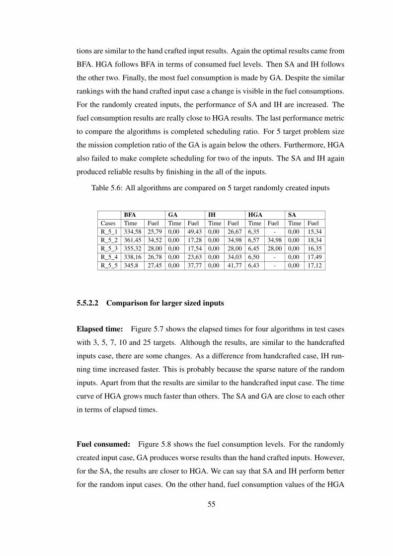
tions are similar to the hand crafted input results. Again the optimal results came from
BFA. HGA follows BFA in terms of consumed fuel levels. Then SA and IH follows
the other two. Finally, the most fuel consumption is made by GA. Despite the similar
rankings with the hand crafted input case a change is visible in the fuel consumptions.
For the randomly created inputs, the performance of SA and IH are increased. The
fuel consumption results are really close to HGA results. The last performance metric
to compare the algorithms is completed scheduling ratio. For 5 target problem size
the mission completion ratio of the GA is again below the others. Furthermore, HGA
also failed to make complete scheduling for two of the inputs. The SA and IH again
produced reliable results by finishing in the all of the inputs.
Table 5.6: All algorithms are compared on 5 target randomly created inputs
BFA GA IH HGA SACases Time Fuel Time Fuel Time Fuel Time Fuel Time FuelR_5_1 334,58 25,79 0,00 49,43 0,00 26,67 6,35 - 0,00 15,34R_5_2 361,45 34,52 0,00 17,28 0,00 34,98 6,57 34,98 0,00 18,34R_5_3 355,32 28,00 0,00 17,54 0,00 28,00 6,45 28,00 0,00 16,35R_5_4 338,16 26,78 0,00 23,63 0,00 34,03 6,50 - 0,00 17,49R_5_5 345,8 27,45 0,00 37,77 0,00 41,77 6,43 - 0,00 17,12
5.5.2.2 Comparison for larger sized inputs
Elapsed time: Figure 5.7 shows the elapsed times for four algorithms in test cases
with 3, 5, 7, 10 and 25 targets. Although the results, are similar to the handcrafted
inputs case, there are some changes. As a difference from handcrafted case, IH run-
ning time increased faster. This is probably because the sparse nature of the random
inputs. Apart from that the results are similar to the handcrafted input case. The time
curve of HGA grows much faster than others. The SA and GA are close to each other
in terms of elapsed times.
Fuel consumed: Figure 5.8 shows the fuel consumption levels. For the randomly
created input case, GA produces worse results than the hand crafted inputs. However,
for the SA, the results are closer to HGA. We can say that SA and IH perform better
for the random input cases. On the other hand, fuel consumption values of the HGA
55

0
20
40
60
80
100
120
3_target 5_target 7_target 10_target 25_target
Ela
pse
d T
ime (
seco
nd
)
Problem Size (targets)
GreedyIntlinprog Heuristic
Simplex HeuristicHybrid Greedy
Figure 5.7: Time consumptions of the algorithms for different size of randomly cre-ated inputs
are still a little bit better than SA and IH.
Scheduling Completion Ratio: Lastly, in Figure 5.9 scheduling completion rates
of the algorithms are provided. GA performs badly for the missions which have time
windows that are sparse. Both GA and HGAs success ratios are falling down in the
larger sized inputs. SA and IH algorithms again seem more reliable for larger sized
inputs. Another interesting point to discuss about this results is for the 25 target case.
The algorithms completion rates are under 40 percent. No complete scheduling would
be possible due to the randomly created inputs but unfortunately there is no optimal
algorithm to test this situation in a this size of a big input.
Lastly, we present a detailed results table for large sized inputs for randomly created
inputs case in the table 5.7. In this table, we compared 4 of the algorithms with a 20
target size large input set. As the input size gets larger, all of the differences between
the result of the algorithms becomes recognizable. HGA took more than 2 minutes to
complete the mission planning. This is far too much for a real time job. Furthermore,
this consumption can grow further with the larger problem instances. IH provided
56
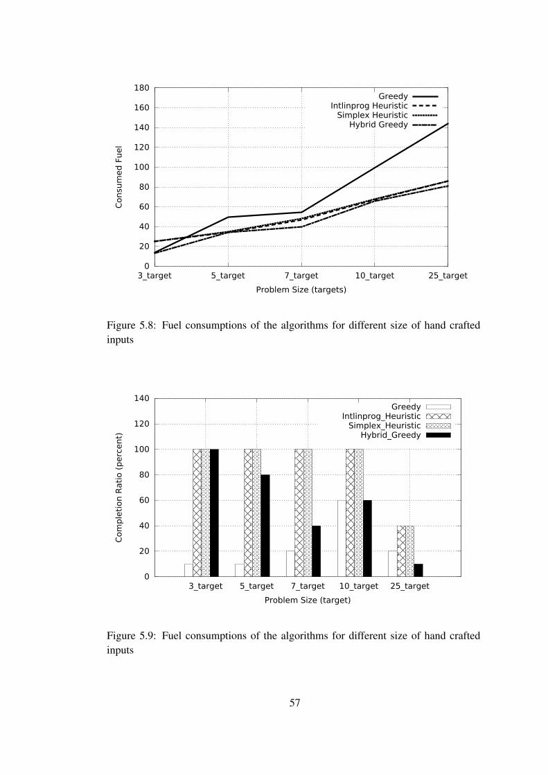
0
20
40
60
80
100
120
140
160
180
3_target 5_target 7_target 10_target 25_target
Consu
med
Fuel
Problem Size (targets)
GreedyIntlinprog Heuristic
Simplex HeuristicHybrid Greedy
Figure 5.8: Fuel consumptions of the algorithms for different size of hand craftedinputs
0
20
40
60
80
100
120
140
3_target 5_target 7_target 10_target 25_target
Com
ple
tion R
ati
o (
perc
ent)
Problem Size (target)
GreedyIntlinprog_Heuristic
Simplex_HeuristicHybrid_Greedy
Figure 5.9: Fuel consumptions of the algorithms for different size of hand craftedinputs
57
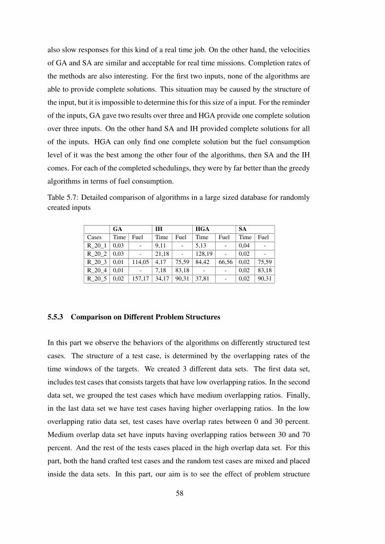
also slow responses for this kind of a real time job. On the other hand, the velocities
of GA and SA are similar and acceptable for real time missions. Completion rates of
the methods are also interesting. For the first two inputs, none of the algorithms are
able to provide complete solutions. This situation may be caused by the structure of
the input, but it is impossible to determine this for this size of a input. For the reminder
of the inputs, GA gave two results over three and HGA provide one complete solution
over three inputs. On the other hand SA and IH provided complete solutions for all
of the inputs. HGA can only find one complete solution but the fuel consumption
level of it was the best among the other four of the algorithms, then SA and the IH
comes. For each of the completed schedulings, they were by far better than the greedy
algorithms in terms of fuel consumption.
Table 5.7: Detailed comparison of algorithms in a large sized database for randomlycreated inputs
GA IH HGA SACases Time Fuel Time Fuel Time Fuel Time FuelR_20_1 0,03 - 9,11 - 5,13 - 0,04 -R_20_2 0,03 - 21,18 - 128,19 - 0,02 -R_20_3 0,01 114,05 4,17 75,59 84,42 66,56 0,02 75,59R_20_4 0,01 - 7,18 83,18 - - 0,02 83,18R_20_5 0,02 157,17 34,17 90,31 37,81 - 0,02 90,31
5.5.3 Comparison on Different Problem Structures
In this part we observe the behaviors of the algorithms on differently structured test
cases. The structure of a test case, is determined by the overlapping rates of the
time windows of the targets. We created 3 different data sets. The first data set,
includes test cases that consists targets that have low overlapping ratios. In the second
data set, we grouped the test cases which have medium overlapping ratios. Finally,
in the last data set we have test cases having higher overlapping ratios. In the low
overlapping ratio data set, test cases have overlap rates between 0 and 30 percent.
Medium overlap data set have inputs having overlapping ratios between 30 and 70
percent. And the rest of the tests cases placed in the high overlap data set. For this
part, both the hand crafted test cases and the random test cases are mixed and placed
inside the data sets. In this part, our aim is to see the effect of problem structure
58
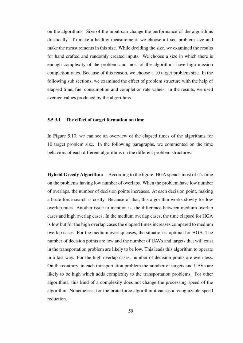
on the algorithms. Size of the input can change the performance of the algorithms
drastically. To make a healthy measurement, we choose a fixed problem size and
make the measurements in this size. While deciding the size, we examined the results
for hand crafted and randomly created inputs. We choose a size in which there is
enough complexity of the problem and most of the algorithms have high mission
completion rates. Because of this reason, we choose a 10 target problem size. In the
following sub sections, we examined the effect of problem structure with the help of
elapsed time, fuel consumption and completion rate values. In the results, we used
average values produced by the algorithms.
5.5.3.1 The effect of target formation on time
In Figure 5.10, we can see an overview of the elapsed times of the algorithms for
10 target problem size. In the following paragraphs, we commented on the time
behaviors of each different algorithms on the different problem structures.
Hybrid Greedy Algorithm: According to the figure, HGA spends most of it’s time
on the problems having low number of overlaps. When the problem have low number
of overlaps, the number of decision points increases. At each decision point, making
a brute force search is costly. Because of that, this algorithm works slowly for low
overlap rates. Another issue to mention is, the difference between medium overlap
cases and high overlap cases. In the medium overlap cases, the time elapsed for HGA
is low but for the high overlap cases the elapsed times increases compared to medium
overlap cases. For the medium overlap cases, the situation is optimal for HGA. The
number of decision points are low and the number of UAVs and targets that will exist
in the transportation problem are likely to be low. This leads this algorithm to operate
in a fast way. For the high overlap cases, number of decision points are even less.
On the contrary, in each transportation problem the number of targets and UAVs are
likely to be high which adds complexity to the transportation problems. For other
algorithms, this kind of a complexity does not change the processing speed of the
algorithm. Nonetheless, for the brute force algorithm it causes a recognizable speed
reduction.
59

Greedy Algorithm: GA worked fast for all of the input types. The structure of the
algorithm does not seem to effect it in terms of time.
Intlinprog Heuristic Algorithm: IH worked fast for the low overlap and medium
overlap rates. For the cases having high overlap rates, the efficiency of the algorithm
is lower compared to other two. In the cases consisting high level of overlaps, there is
a possibility to have low number of decision points. Low decision points yields low
number of and fairly large sized transportation problems. IH solves transportation
problem but it is not a very fast approach. Hence, large sized transportation problems
seems to be effecting the speed of IH.
Simplex Heuristic Algorithm: Similar to GA, SA did not effected much by the
structure of the algorithm. For the high overlap cases, the size of the transportation
algorithm increases. SA solves transportation algorithm fast. So, this increase did not
effect the overall spent time much. Still, it is possible to recognize a small increase
of time in the high overlap cases.
0
5
10
15
20
25
low_overlap medium_overlap high_overlap
Ela
pse
d T
ime (
seco
nd
)
Overlap Ratio (percent)
GreedyIntlinprog Heuristic
Simplex HeuristicHybrid Greedy
Figure 5.10: Figure showing a diagram showing time elapsed in seconds for each ofthe different problem structures for algorithms.
60

5.5.3.2 The effect of target formation on fuel consumption
In the Figure 5.11, fuel consumption levels of the algorithms are provided. In the fig-
ure, we can recognize that all of the algorithms are getting close to each other in the
high overlap case. The reason of this is, the similar infrastructures of the algorithms
designed. All of the algorithms in this thesis are implemented with similar infrastruc-
tures. Because of this, for the high overlap case they give similar responses. They
can find different solutions to transportation problem but the number of transportation
problems are low for this problem formation. This, causes them to find similar results.
Apart from that, algorithms fuel consumption levels does not seem to be effected by
the target formations.
0
20
40
60
80
100
120
140
low_overlap medium_overlap high_overlap
Consu
med
Fuel
Overlap Ratio (percent)
GreedyIntlinprog Heuristic
Simplex HeuristicHybrid Greedy
Figure 5.11: Figure showing a diagram showing consumed fuel levels of the algo-rithms on various different problem structures
5.5.3.3 The effect of target formation on mission completion rates
In Figure 5.12, scheduling completion rates of the algorithms on different target struc-
tures are provided. The results shows that, all of the algorithms are effected from the
low overlap ratio. GA is effected more than the others. The reason is already ex-
61
plained before. When the targets are sparse and there are time differences between
the time windows of the targets, the wrong choices of the GA ends up with incom-
plete scheduling. The reason of providing bad results for the low overlap rates is same
with GA for all the other algorithms. Because, all the other algorithms implemented
have greedy natures. After the dividing process, best results for the transportation
problems are searched. This makes other algorithms a special version of the GA. So,
sometimes they effected from the problem structure in the same way as GA.
0
20
40
60
80
100
120
140
low_overlap medium_overlap high_overlap
Com
ple
tion R
ati
o (
perc
ent)
Overlap Rate (percent)
GreedyIntlinprog_Heuristic
Simplex_HeuristicHybrid_Greedy
Figure 5.12: Figure showing a diagram showing scheduling completion rates of thealgorithms on various different problem structures
The results shows that the best approach for this problem is SA. For small sized
inputs, HGA finds results closer to BFA but for larger inputs, working time of the al-
gorithm is too much. Furthermore, for large size inputs the ratio of finding a complete
scheduling is low for HGA. GA is a faster choice but the fuel consumption values for
the large size inputs is worse than the SA values. IH always finds the same results
with SA but it is significantly slower than SA for large size inputs. SA, is the best
alternative in terms of reliability efficiency and effectiveness.
62

CHAPTER 6
CONCLUSION AND FUTURE WORK
6.1 Conclusions
In this thesis we worked on multiple UAV scheduling and target assignment problem.
The main idea was to approach a divide and conquer type of idea. We wanted to
divide this complex problem into multiple small problems which we know how to
solve. So, the main consideration after this point was to how to divide the problem
and then how to solve the sub problems. The constraint that effects the solutions most
is the time windows for this problem. Targets’ time windows defines a time period
for each target and intersection amounts of the time windows affects’ the possible
complete schedulings for the mission. So, dividing procedure to group the targets
according to their time windows is developed.
After making a division, according to time windows, the small problems created are
started to look like transportation problems. For each of the clusters created, trans-
portation problem is solved. In order to solve the transportation problem, 3 different
approaches were created. The first one is the linear programming method. The sec-
ond approach is solving the small problems with the help of simplex algorithm. Last
approach is solving the small problem instances with brute force algorithm. Further-
more, to see the effectiveness and the solution quality of these 3 different methods a
brute force and a greedy algorithm is also developed.
The five algorithms developed are tested with various different data. There were two
main test beds. First one was the hand crafted inputs and the second class of test
cases were randomly created inputs. The algorithms are tested with the inputs from
63

3 targets size to 25 targets size and evaluated according to 3 different performance
metrics. These performance metrics are elapsed time, fuel consumption as a cost
measurement and lastly the rate of complete scheduling to see the reliability of the
algorithms.
Despite the fact that brute force algorithm always finds the optimal solutions it is too
slow to be feasible. To be able to find the optimal results it tries to search a big part
of the solution space. For this kind of a NP-Hard problem this yields a too complex
solution. This problem is usually needed for real time applications and for a real time
application this much running time is not suitable.
Greedy algorithm provides fast results independent from the size of the problem set.
Although being fast is important for real time problems, the failure rate of the greedy
algorithm is too much for a critical mission. Furthermore, for the large input sizes the
quality of the solutions created by the greedy algorithm was lower than the other tried
approaches.
Intlinprog heuristic is a similar method to our solution. The only difference from
our algorithm was the solution method of the small transportation problems. This
approach solves the transportation problems with linear programming. Linear pro-
gramming is fast enough for solving one transportation problem but it is slower than
simplex algorithm. As the number of small transportation problems increases this
small difference between the working times gets larger.
After comparing the all of the implemented approaches with the data sets, we can
say that the most suitable algorithm from this 5 algorithms for UAV mission planning
problem is the simplex heuristic method. It provides fast, reliable and acceptable
solutions in a fast fashion.
6.2 Future Work
In this thesis an UAV mission planning problem with multiple constraints is solved.
The main constraints were the fuel capacity of UAVs, capacity of targets, time win-
dows of the targets and minimum cost. Some more constraints can be added to this
64

problem to make it more realistic.
In this thesis all of the UAVs were identical and there were no constraints for UAVs
that limits their movement. This kind of constraints can be added to achieve more
realistic UAV design. For instance, minimum segment length constraint, minimum
turning angle constraint, maximum diving angle constraint and heterogeneous UAVs
[33] are different ideas that can be added to achieve a more realistic UAV design.
Another idea can be to simulate a more realistic environment. For this study there
were no constraints in the environment and the environment was 2D. In the environ-
ment there can be some obstacles or no flight zones or some critical regions. Fur-
thermore a 3D environment design can be developed. These constraints can also be
added to achieve a realistic environment design.
65

66
REFERENCES
[1] Umanned aerial vehicle in logistics- a dhl perspective on implications and usecases for the logistics industry, 2014.
[2] S. M. Adams and C. J. Friedland. A survey of unmanned aerial vehicle (uav)usage for imagery collection in disaster research and management. In Proceed-ings of the 9th International Work Shop on Remote Sensing for Disaster Re-sponse,(2011)., 2011.
[3] R. AI-Tahir and M. Arthur. Unmanned aerial mapping solution for small islanddeveloping states. In Proceedings of Global Geospatial Conference 2012, 2012.
[4] M. Alighanbari and J. P. How. Cooperative task assignment of unmanned aerialvehicles in adversarial environments. In American Control Conference PortlandUS, 2005.
[5] M. Alighanbari, Y. Kuwata, and J. P. How. Coordination and control of multipleuavs with timing constraints and loitering. In American Control Conference,2003. Proceedings of the 2003, volume 6, pages 5311 – 5316, 2003.
[6] J. Allen and B. Walsh. Enhanced oil spill surveillance, detection and moni- tor-ing through the applied technology of unmanned air systems. In Internationaloil spill conference, pages 113–120. American Petroleum Institute, 2008.
[7] J. b. Brachet, R. Cleaz, A. Denis, A. Diedrich, D. King, P. Mitchell, D. Morales,J. Onnée, T. Robinson, O. Toupet, B. Wong, J. b. Brachet, R. Cleaz, A. Denis,A. Diedrich, D. King, P. Mitchell, D. Morales, J. Onnée, T. Robinson, O. Toupet,B. Wong, and T. Contents. Reference material for a proposed formation flightsystem, 2005.
[8] J. S. Bellingham. Coordination and control of uav fleets using mixed-integerlinear programming. Masters thesis, Department of Aeronautics and Astronau-tics - Massachusetts Institue of Technology, 2002.
[9] B. Chandran and S. Raghavan. Modeling and solving the capacitated vehiclerouting problem on trees. The Vehicle Routing Problem: Latest Advances andNew Challenges Operations Research/Computer Science Interfaces, 43:239–261, 2008.
[10] Y. Chang and L. Chen. Solve the vehicle routing problem with time windows viaa genetic algorithm. In Discrete and Continious Dynamical Systems Supplement2007, 2007.
67

[11] X. Cheng, D. Cao, and C. Li. Survey of cooperative path planning for multipleunmanned aerial vehicles. Applied Mechanics Materials, 2014(667-679):388,2014.
[12] T. Chou, M. Yeh, Y. Chen, and Y. Chen. Disaster monitoring and managementby the unmanned aerial vehicle technology. In ISPRS TC VII Symposium, 2010.
[13] T. Coffey and J. A. Montgomery. The emergence of mini uavs for militaryapplications. Defense Horizons, December 2002(22), 2002.
[14] A. Dang and J. Horn. Formation control of leader-following uavs to track amoving target in a dynamic environment. Journal of Automation and ControlEngineering, 3, 2015.
[15] M. Desroches, J. K. Lenstra, M. V. P. Savelsberg, and F. Soumis. Vehicle rout-ing with time windows: Optimization and approximation. In Vehicle routingmethods and studies, 1988.
[16] X. C. Ding, A. Rahmani, and M. Egerstedt. Optimal multi-uav convoy protec-tion. IEEE Transactions on Robotics, 26(2):256–268, 2010.
[17] J. Doebbler, P. Gesting, and J. Valasek. Real time path planning and terrainobstacle avoidance for general aviation aircraft. In AIAA Guidance, Navigation,and Control Conference and Exhibit, August 2005.
[18] A. Dogan. Probabilistic approach in path planning for uavs. In Proceedings ofthe 2003 IEEE International Symposium on Intelligent Control, 2003.
[19] B. Dorronsoro. A grid-based hybrid cellular genetic algorithm for very largescale instances of the cvrp. In 21ST European Conference on Modeling andSimulation ECMS 2007, pages 759–765, 2007.
[20] D. Edwards, T. Bean, D. Odell, and M. Anderson. A leader-follower algorithmfor multiple auv formations. In Autonomous Underwater Vehicles, 2004.
[21] W. Eggers and M. H. Draper. Multi-uav control for tactical reconnaissanceand close air support missions: Operator perspectives and design challenges.In Human Factors and Medicine Panel of the NATO Research and TechnologyOrganization, 2006.
[22] J. J. Enright, E. Frazzoli, M. Pavone, and K. Savla. Uav routing and coordi-nation in stochastic, dynamic environments. Handbook of Unmanned AerialVehicles, pages 2079–2019, 2014.
[23] Y. Eun and H. Bang. Cooperative control of multiple unmanned aerial vehiclesusing the potential field theory. Journal of Aircraft, 43, 2006.
68

[24] M. Faied, A. Mostafa, and A. Girard. Vehicle routing problem instances: Ap-plication to multi-uav mission planning. In AIAA Guidance, Navigation, andControl Conference, August 2010.
[25] M. Freed, R. Harris, and M. Shafto. Comparing methods for uav-based au-tonomous surveillance. In National Conference on Artificial Intelligence, 2004.
[26] L. Geng, Y. F. Zhang, J. J. Wang, J. Y. H. Fuh, and S. H. Teo. Mission planningof autonomous uavs for urban surveillance with evolutionary algorithms. In10th IEEE International Conference on Control and Automation (ICCA), 2013.
[27] A. Geramifard, J. Redding, N. Roy, and J. P. How. Uav cooperative control withstochastic risk models. In American Control Conference (ACC), 2011.
[28] D. Glade. Unmanned aerial vehicles: Implications for military operations.Technical report, Air Univ. Press Maxwell Afb Al, July 2000.
[29] W. Guo. Optimal uav flights for seeability and endurance in winds. Mastersthesis, The Graduate School of the University of Minnesota, December 2010.
[30] L. S. J. Tian and Y. Zheng. Genetic algorithm based approach for multi-uav co-operative reconnaissance mission planning problem. Foundations of IntelligentSystems Lecture Notes in Computer Science, 4203, 2006.
[31] Y. Jin, A. A. Minai, and M. M. Polycarpou. Cooperative real-time search andtask allocation in uav teams. In Proceedings of the 42nd IEEE Conference onDecision and Control Maui, Hawaii USA, 2003.
[32] W. A. Kamal, D. Gu, and I. Postlethwaite. A decentralized probabilistic frame-work for the path planning of autonomous vehicles. In IFAC World Congress,volume 16, 2005.
[33] W. A. Kamal and R. Samar. A mission planning approach for uav applications.In Proceedings of the 47th IEEE Conference on Decision and Control, 2008.
[34] S. Karaman, T. Shima, and E. Frazzoli. Task assignment for complex uav op-erations using genetic algorithms. In AIAA Guidance, Navigation, and ControlConference Chicago Illinois, August 2009.
[35] J. Kim and J. R. Morrison. On the concerted design and scheduling of multipleresources for persistent uav operations. Journal of Intelligent Robotic Systems,74:479–498, 2013.
[36] D. B. Kingston and C. J. Schumacher. Time-dependent cooperative assignment.In 2005 American Control Conference, 2005.
[37] J. W. Langelaan. Long distance/duration trajectory optimization for small uavs.In Guidance, Navigation and Control Conference, Hilton Head, South Carolina,August 2007.
69

[38] H. C. Lau, M. Sim, and K. M. Teo. Vehicle routing problem with time windowsand a limited number of vehicles. European Journal of Operational Research,pages 559–569, 2003.
[39] N. H. M. Li and H. H. T. Liu. Multiple uavs formation flight experiments usingvirtual structure and motion synchronization. In AIAA Guidance, Navigation,and Control Conference, 2009.
[40] R. Mark. Unmanned aerial vehicle contributions to intelligence, surveillance,and reconnaissance missions for expeditionary operations. Masters thesis,Naval Postgraduate School Monterey, CA, September 2004.
[41] MathWorks. Optimization modeling 2: Converting tosolver form. http://www.mathworks.com/videos/optimization-modeling-2-converting-to-solver-form-101560.html. Online, accessed 17 August 2015.
[42] J. Ondrácek. Intelligent algorithms for monitoring of the environment aroundoil pipe systems using unmanned aerial systems. Master’s thesis, Czech Tech-nical University in Prague, May 2014.
[43] Y. B. Park and S. C. Hong. Performance evaluation of vehicle routing heuristicsin a stochastic environment. International Journal of Industrial Engineering:Theory, Applications and Practice, 10:435–441, 2003.
[44] Z. Peng, D. Wang, W. Lan, X. Li, and G. Sun. Decentralized cooperative con-trol of autonomous surface vehicles with uncertain dynamics: a dynamic surfaceapproach. In 2011 American Control Conference on O’Farrell Street, San Fran-cisco, CA, USA, 2011.
[45] C. Rasche, C. Stern, L. Kleinjohann, and B. Kleinjohann. Role-based path plan-ning and task allocation with exploration tradeoff for uavs. In 11th Int. Conf.Control, Automation, Robotics and Vision Singapore, 2010.
[46] S. Rasmussen. Optimal vs. heuristic assignment of cooperative autonomousunmanned air vehicles. In AIAA Guidance, Navigation, and Control Conferenceand Exhibit, 2003.
[47] S. J. Rasmussen and T. Shima. Branch and bound tree search for assigning co-operating uavs to multiple tasks. In Proceedings of the 2006 American ControlConference, 2006.
[48] T. Schouwenaars, B. Moor, E. Feron, and J. How. Mixed integer programmingfor multi-vehicle path planning. In European Control Conferance, volume 1,pages 2603–2608, 2001.
[49] G. Sequeira. Vision based leader follower formation control for mobile robots.Masters thesis, University of missuri rolla, 2007.
70

[50] T. Shima, S. J. Rasmussen, and A. G. Sparks. Uav cooperative multiple taskassignments using genetic algorithms. In American Control Conference, 2005.
[51] T. Shima, S. J. Rasmussen, A. G. Sparks, and K. M. Passino. Multiple task as-signments for cooperating uninhabited aerial vehicles using genetic algorithms.Computers Operations Research, 33, 2006.
[52] T. Skrzypietz. Unmanned Aircraft Systems for Civilian Missions, volume 1.Brandenburgisches Institut für Gesellschaft und Sicherheit (BIGS), bigs policypaper edition, 2012.
[53] D. M. Sobers. Efficient ranging-sensor navigation methods for indoor aircraft.PhD thesis, Georgia Institute of Technology, August 2010.
[54] T. Soleymani and F. Saghafi. Behavior-based acceleration commanded forma-tion flight control. In International Conference on Control, Automation andSystems, 2010.
[55] L. Sorbi, G. D. Capua, J. Fontaine, and L. Toni. A behavior-based missionplanner for cooperative autonomous underwater vehicles. International Journalof Industrial Engineering: Theory, Applications and Practice, 46:32–44, 2012.
[56] F. Takes. Applying monte carlo techniques to the capacitated vehicle routingproblem. Masters thesis, Leiden University, The Netherlands, February 2010.
[57] J. Wu, Z. Peng, and J. Chen. 3d multi-constraint route planning for uav low-altitude penetration based on multi-agent genetic algorithm. In 18th IFAC WorldCongress Milano (Italy), 2011.
[58] P. Yan, M. Ding, and C. Zheng. Mission adaptable-route planning in uncertainand adversarial environments. International Journal of Artificial IntelligenceTools, 15(5):803–821, 2006.
[59] Z. Yongjia and D. Shuling. Unmanned aircraft vehicle path planning based onimage skeleton and greedy algorithm. Journal of BUAA (Natural Science), 36,2010.
[60] C. Zhou, M. Ding, and C. Zheng. Real-time route planning for unmanned airvehicle with an evolutionary algorithm. International Journal of Patter Recog-nition and Artifical Intelligence, 17(1):63–81, 2003.
71