tax’ - london school of economicsdarp.lse.ac.uk/papersdb/ivanova-keen-klemm_(ep05).pdf · tax...

Economic Policy July 2005 Printed in Great Britaincopy The Institute For Fiscal Studies 2005

Russiarsquos lsquoflat taxrsquo

Blackwell Publishing LtdOxford UKECOPEconomic Policy0266-4658copy CEPR CES MSH 200543Original ArticleRUSSIArsquoS lsquoFLAT TAXrsquo

ANNA IVANOVA MICHAEL KEEN and ALEXANDER KLEMM

The Russian lsquoflat taxrsquo reform

SUMMARY

In 2001 Russia dramatically reduced its higher rates of personal income tax(PIT) establishing a single marginal rate at the low level of 13 In the followingyear real revenue from the PIT increased by about 26 This lsquoflat taxrsquo experiencehas attracted much attention (and emulation) making it perhaps the most importanttax reform of recent years But it has been little studied This paper asks whetherthe strong performance of PIT revenue was itself a consequence of this reformusing both macro evidence and in particular micro level data on the experiencesof individuals and households affected by the reform to varying degrees It concludesthat there is no evidence of a strong supply side effect of the reform Compliancehowever does appear to have improved quite substantially ndash by about one thirdaccording to our estimates ndash though it remains unclear whether this was due to theparametric tax reform or to accompanying changes in enforcement

mdash Anna Ivanova Michael Keen and Alexander Klemm

RUSSIArsquoS lsquoFLAT TAXrsquo 399

Economic Policy July 2005 pp 397ndash444 Printed in Great Britaincopy CEPR CES MSH 2005


Anna Ivanova Michael Keen and Alexander Klemm

International Monetary Fund International Monetary Fund Institute for Fiscal Studies and University College London

1 INTRODUCTION

At the start of 2001 Russia unified its marginal rates of personal income taxation ndashpreviously at 12 20 and 30 ndash at the single rate of 13 In the year following theadoption of this lsquoflat taxrsquo

1

revenue from the personal income tax (PIT) increased byabout 46 (about 26 in real terms) relative to GDP PIT revenues increased bynearly one-fifth Such a strong revenue performance following a marked reduction ofmarginal tax rates quickly attracted attention and emulation in East Europe While theBaltic countries had preceded Russia in introducing single rate income tax structures

2

We thank Richard Blundell Dale Chua Bob Conrad Gohoon Kwon Victoria Perry Ian Preston John Odling Smee NienkeOomes David Owen Pierre Pestieau Carlos Silvani Stephen Smith Antonio Spilimbergo Victor Thuronyi Andreacutes Velascoand participants at the panel meeting for comments and suggestions Opinions expressed here are those of the authors and donot necessarily represent the views or policy of the IMF nor those of the Institute for Fiscal Studies which has no corporateviews At the IFS the work was partially funded by the ESRC Centre for the Microeconomic Analysis of Public Policy

The Managing Editor in charge of this paper was Paul Seabright

1

This term has come to be used extremely loosely The Russian version was not a flat tax in the sense of Hall and Rabushka(1995) which is essentially an expenditure tax implemented by combining a flat tax on wage income and a cash flow businesstax levied at the same rate (although Rabushka (2003) has spoken positively of the Russian experience) More generally thevarious lsquoflat taxesrsquo adopted in Russia and elsewhere differ quite markedly from one another including in whether the rate ofcorporation tax (or even VAT) is aligned with that of the PIT (with the Russian variant in this respect being one of the lessdramatic reforms) Hence the inverted commas in our title

2

Outside Europe Bolivia has had such a tax system since 1986 Other small states and territories (such as Jersey) have had flatrate income taxes for decades

400 ANNA IVANOVA MICHAEL KEEN AND ALEXANDER KLEMM

ndash Estonia leading the way in 1994 ndash the Russian experience was clearly the mostinfluential It was followed by the adoption of various forms of flat tax ndash the commonelement being a single low marginal rate of PIT ndash in Serbia the Ukraine andSlovakia (in 2003) and most recently by Georgia and Romania (in 2005) with ratesranging from 12 (Georgia) to 19 (Slovakia) Similar reforms have been underconsideration in Belarus Guatemala the Kyrgyz Republic El Salvador Paraguayand Poland

3

More recently the lsquoflat taxrsquo has come to feature prominently in policydebates in Western Europe and the United States

4

The Russian reform has thuscome to be extraordinarily influential making it arguably the most important taxreform of the last decade

Given the importance of the reform not only for Russia itself but also for the manycountries that have adopted or are considering adopting similar measures it isclearly important to understand the experience there and the lessons that canappropriately be drawn from it Did the reform indeed have the strong positiveeffects on compliance andor labour supply (especially the former) that its advocateshave claimed Were these effects even so strong that the lower tax rates lsquopaid forthemselvesrsquo

The purpose of this paper is to address these and related questions both by takinga macroeconomic perspective on wider revenue developments at this time and inparticular by using the individual- and household-level panel data that are nowavailable in the Russian Longitudinal Monitoring Survey (RLMS) spanning pre- andpost-reform periods to provide a clear assessment of the impact of the reform on taxrevenue work effort wage rates and taxpayer compliance

Though it has been much commented on and admired the Russian experiencehas been subject to very little rigorous empirical analysis

5

The only econometricanalysis of which we are aware is presented in a series of papers from the Institutefor Economies in Transition The empirical strategy in this work ndash as in Sinelnikov-Mourylev

et al

(2003)

6

for instance ndash has been to use the RLMS to constructobservations at the level of the regions of Russia and ask whether the implied PITbase has increased more in those regions where the weighted average marginal taxrate was most reduced The conclusion drawn is that there has indeed been a signif-icant effect of this sort with the authors ultimately attributing about half of therevenue gain to the reduction in marginal rates Though striking these results aresubject to a number of limitations It could be the case for instance that thoseregions in which the proportion of incomes subject to the higher rates of tax prior toreform was greatest were also systematically those which saw for some reason the

3

As a variant Armenia has redesigned its progressive PIT and regressive social insurance schedule so that the combination ofthe two has a single positive marginal rate

4

See for example the positive assessment in

The Economist

of 14 April 2005 A useful summary of recent flat tax proposals isin Grecu (2004)

5

Informal accounts are provided in IMF (2002) and Chua (2003)

6

See also Chapter 4 of Glavatskaya and Seryanova (2003)


greatest increase in the incomes of those subject to essentially the same marginal ratebefore and after reform (and hence also the greatest increase in the tax base) Micro-levelpanel data are needed to identify such possibilities offering potentially the best basisupon which to assess the implications of the reform That is the approach pursued here

The concern in this paper it should be stressed is solely with positive aspects ofthe reform in terms of its impact on revenue compliance and labour supply we donot attempt to gauge the extent of any efficiency or welfare gains or to evaluate itsdistributional impact

7

The focus is also only on relatively short-term effects thoughit could be that full supply responses to the reform occur only after some time eitherbecause of market rigidities or because the reform was not initially perceived as permanent

The structure of the paper is as follows Section 2 describes the PIT and (importantin understanding its effects) related tax reforms in 2001 Section 3 briefly reviews thelessons of theory as to the likely effects of the reform and Section 4 takes a macroperspective on the assessment of the reform The main analysis based on micro paneldata is in Section 5 which describes the data and methodology used and in Section6 which reports results Section 7 concludes

2 PIT AND THE 2001 TAX REFORMS

This section describes the PIT reform and other tax changes that took place aroundthe same time

21 Reform of the taxation of income

The change in the rate structure of the PIT which took effect on 1 January 2001 issummarized in Table 1

The threshold level of taxable income at which the higher rates began prior toreform was high about 187 of the average wage in 2000 It should be noted toothat although the basic exemption grew by 30 in real terms between 2000 and2001 it remained roughly unchanged relative to the average wage (at about 12)

8

Strictly the post-reform PIT was not a single rate tax since some kinds of incomendash from gambling lottery prizes some insurance payments the benefit from loansobtained at less than market rates

9

and lsquoexcessiversquo bank interest

10

ndash were taxed at

7

Sinelnikov-Mourylev

et al

(2003) argue that reduced evasion (and hence higher tax payments) by higher-rate taxpayers actuallyincreased the effective progressivity of the PIT with respect to wage income (while finding no conclusive result for its progressivitywith respect to total income)

8

Both before and after reform this allowance was withdrawn in discrete jumps at higher levels of income (as described in thedata appendix) This is taken fully into account in the empirical analysis reported below but for simplicity ignored in thediscussion that follows and in Table 1 and Figure 1

9

This was calculated as the difference between the interest implied by the market rate (calculated as 75 of the Central Banksrsquorefinancing rate on the date of receipt of a ruble loan or 9 for loans received in foreign currency) and that actually paid

10

Bank interest became taxable if paid at a rate exceeding 75 of the Central Banksrsquo refinancing rate on ruble deposits or 9on foreign currency deposits Since most deposits earned less than this interest income was generally untaxed


35 approximating combined rates of the PIT and unified social tax (discussedbelow) in an attempt to close popular avoidance schemes (some of which showedimpressive adroitness)

11

For similar reasons dividends were taxed at 30 (up from15 in 2000) but with the introduction of a non-refundable credit for underlyingCIT paid

There were also changes in 2001 to the base of the PIT with the elimination ofvarious exclusions for military servicemen and expatriates and the introduction of asimplified system of deductions (standard social property and professional) More-over there was a modification of the agreement for sharing PIT revenue betweenfederal and regional governments in 2000 regional governments received only 80of PIT revenues from 2001 they received 100 This may have strengthened thecollection incentive of regional governments

Importantly however these changes to the PIT structure were not the only taxreform at this time Most significant for present purposes Part II of the new tax codealso significantly altered the structure of social insurance payments as shown inTable 2 Prior to the reform separate contributions were paid to the pension socialmedical and employment funds at a combined rate at all income levels of 385on the employer and 1 on the employee (this last to the pension fund) After thereform a single lsquounified social taxrsquo (UST) was charged on the employer ndash for firmsmeeting various additional requirements

12

ndash at marginal rates decreasing from 356to 5 with the lowest marginal rate applying to salaries in excess of (the very highlevel of ) 600000 rubles

11

Under one scheme for instance the enterprise purchased insurance against a very low probability event (deducting itspremiums) At the same time its employees entered a contract with the same insurance company for a very high probabilityevent Employees thus received compensation in the form of an insurance payout which was not taxable

12

To qualify for the regressive rate the average payment per employee had to be above a threshold (2500 rubles in 2001) whena certain number of employees with the highest incomes were excluded from the calculation The rationale for this wasapparently to encourage compliance on a broad base by denying benefit to firms that declared only a few highly paidindividuals Moreover to discourage income shifting the regressive social scheme in 2001 could be applied only by taking intoaccount average payment per employee in 2000

Table 1 The PIT rate structure before and after reform

Marginal rate before reform (2000) After reform (2001)

Bracket (rublesa) Rate Bracket (rubles) RateBelow 3168 0 Below 4800 03168 to 50000 12 Above 4800 1350000 to 150000 20Above 150000 30

a For comparison the average annual salary was 26676 rubles in 2000 and 39384 rubles in 2001 The officialexchange rate expressed in rubles per US dollar was 2813 in 2000 and 2917 in 2001

Source Russian Tax Code Part II


The combined effect of both reforms on effective marginal tax rates is shownin Figure 1 which plots marginal tax rates before and after the reform against theincome level For those initially paying PIT at the lower rate of 12 ndash a particularlyimportant group for our later analysismdashthe net effect of the 2001 reforms was areduction in the combined marginal rate of PIT and social insurance of about 13percentage points

13

13

Because the social taxes are charged on a tax-exclusive basis this is calculated as the difference between (012

+

001

+

0385)(1385) and (013

+

0356)(1356)

Table 2 Social tax rate structure before and after reforma

Legal incidence

Before Reform (2000) After Reform (2001)

Income range Marginal rate Income range Marginal rate

Employee All 1 All 0Employer All 385b Below 100000 356

100000ndash300000 20300000ndash600000 10Above 600000 5 (from 2002 2)

a Different rates apply to agricultural workers lawyers self-employed and Northern ethnic communities Insome regions some additional charges were levied for instance in Moscow an Education Levy of 1b This was made up of contributions to the Pension Fund (28) Social Insurance Fund (54) State EmploymentFund (15) and Medical Insurance Fund (36)


Figure 1 Marginal tax rates (including social taxes) before and after the reform

Note The density shown is the kernel of the distribution of gross incomes in 2000 One individual reporting earnings of 2353564 rubles was dropped to improve clarity of the chart (This individual did not participate in the 2001 survey so is not included in the regression analysis either)


22 Other tax changes

Several other tax changes that also took effect at the start of 2001 are summarizedin Table 3

Tax administration was also undergoing significant change at the time of the PITreform as described in Chua (2003) Through the latter 1990s there is no doubt thatthe system was in something close to chaos with very poor compliance widespreaduse of tax offsets and difficult relations between levels of government Gaddy andGale (2005) cite estimates that in the mid-1990s only 8 of large enterprises paidtheir tax bills in cash 63 effectively paid in kind and the rest did not pay at allBrooks (2001) quotes an estimate that 90 of private sector income was concealedfrom the tax authorities and reports dramatic difficulties in collecting tax on the other10 in 1996 lsquo26 tax collectors were killed 74 were injured in the course of theirwork 6 were kidnapped and 41 had their homes burnt downrsquo Salaries of tax officialswere very low contributing to an environment of corrupt practices and further under-mining respect for government and tax administration

Part I of the new tax code which became effective on 1 January 1999 sought athorough modernization of tax administration It provided for the introduction of acommon taxpayer identification number and allowed in certain cases for the indirectassessment of tax liability More authority was also given to the State Tax Service inparticular in allocating income deductions and credits across related taxpayers andin enforcing debt repayments by liquidated companies Importantly Part I also elim-inated a ceiling on interest charged on overdue taxes Some of its provisions however

Table 3 Major other changes in Russian Federation tax code in 2001

Type of tax Rate Base Other changes

Corporate Income Tax

Combined maximum rate increased from 30 to 35

Federal rate (11) and regional rate (up to 19) remained unchanged but municipalities were allowed to impose an additional rate of 5

Value Added Tax

No changes Scaling back of exemptions including a narrowing of the exemption for pharmaceuticals

a) Shift from the origin to the destination basis for trade with other CIS countries (except Belarus and on energy) b) adoption of measures directed at reducing the compliance burden for small traders

Turnover taxes

The Social Infrastructure Maintenance Tax of 15 was abolished and the Road User Tax reduced from 25 to 15


worked in the opposite direction for example tax obligations were deemed dis-charged once the taxpayer had provided a payment order to a bank which allowedtaxpayers to claim fulfilment of their obligations without actually paying any taxOn balance the general thrust of the administrative reforms at this time was tostrengthen the effectiveness and powers

14

of the tax administration ndash at least poten-tially In the oil sector there are signs of strengthened enforcement including ameeting between President Putin and 21 leading oil oligarchs to discuss the passageof new laws designed to curtail the use of tax avoidance schemes (Desai

et al

2004)But how and when the reforms in the legal framework and political environmentchanged practice through the wider tax system is very hard to judge we have notbeen able to find any direct evidence on this and opinions on how much actuallychanged at this time do vary

There was thus much more going on at the start of 2001 than simply the changein the rate structure of the PIT One key implication is that it is difficult to isolateeffects of the PIT reform alone The reductions in social insurance taxes in particularwould be expected to trigger quite similar behavioural responses making it especiallydifficult to disentangle the two

3 PREDICTIONS OF THEORY

To provide a stylized framework for coming to grips with the anatomy of the 2001reform write revenue from the personal income tax

R

as

τ

λ

wL

where

τ

denotesthe (tax-exclusive) tax rate

λ

the ratio of declared taxable income to true taxableincome (so describing the degree of compliance with

λ

=

1 corresponding to fullytruthful reporting)

w

the gross wage rate and

L

the level of employment (hereabstracting for simplicity from capital income components of the PIT base)Denoting proportionate changes by hats the revenue effect of any reform is thenapproximated by

reg

asymp

3

+

+

w

+

L

(1)

Though some elements of the 2001 PIT reform tended to increase revenue atunchanged behaviour these ndash though certainly important for some individuals ndash wererelatively minor (the most important probably being the elimination of the exemptionfor military servicemen) Thus the reform corresponds for those initially paying PITat a higher rate to a substantial reduction in

τ

The question is whether the three typesof response to the reform remaining on the right of (1) could have led to such an increasein the tax base as to account to any substantial degree for the strong performanceof PIT revenue subsequent to the reform The rest of this section considers each in

14

In particular the tax police were authorized to conduct tax audits if sufficient evidence of a suspected tax crime was availableand to investigate non-tax commercial crimes such as money laundering


turn and the possibility that the reform may have led to some income-shifting betweenthe CIT and PIT

31 Gross wage rates

In the formal sector one would expect the gross wage

w

to fall as a consequence ofthe reduced tax wedge (both PIT and social taxes)

15

Translated into the terms of theempirical exercise below the implication is that gross wage rates of groups mostaffected by the reform should have fallen relative to those of groups less affected Inthe informal sector the gross wage might conceivably have risen (in order to leavetake-home wages in line with those available in the formal sector) but this wouldhave had no direct impact on tax revenue

32 Work effort

Effects on labour supply might be expected from both the change in gross wage ratesand the change in the parameters of the PIT and social taxes The former dependsroutinely on the elasticity of labour supply so the latter is the focus here

To simplify imagine a reform that leaves the exempt amount and starting marginalrate of tax unchanged but lowers to the same level the (single) top rate (In factas seen above the starting marginal rate ndash inclusive of social insurance ndash fell by 13percentage points and the pattern of effects at the higher rate was more diverse) Asshown in Figure 2

16

by reducing the higher marginal rate to the level of the standardrate the reform has the effect of rotating the budget constraint relating before- andafter-tax income anti-clockwise around the kink point (at the level of income at whichthat higher rate initially applied) until the budget constraint becomes a straightline

15

Take for instance the natural benchmark case of a competitive labour market characterized by equality between the demandfor labour

D(w)

and the supply of labour

S

[

w

(1

minus

λτ

)] (taken to depend on the wage net of taxes actually paid so ignoringfor simplicity the risks associated with non-compliance) Denoting the elasticities of labour demand and supply by

e

D

and

e

S

(both defined to be positive numbers) it is then routine to show that

so that the gross wage falls unless compliance increases by a greater proportion than the tax rate falls Using this relationship(and now ignoring counter-factually but for clarity the social taxes that would also be expected to affect net wage and hencelabour supply) it is straightforward to show that in this simple framework the overall effect on PIT revenue is

A necessary condition for revenue to increase (given

3

+

lt

0) is thus that the elasticity of labour demand exceed unity Giventhis the increase is larger the greater is the elasticity of the supply of labour the higher is the tax rate and the higher is theinitial level of compliance

16

After-tax income on the vertical axis corresponds to consumption and pre-tax income on the horizontal axis is proportional(assuming that the gross wage rate is independent of hours worked) to labour supply So the figure just shows the consumerrsquoschoice between consumption and leisure

w

( )=+

minus

+e

e e

S

S D

λτλτ1

3

reg 3 ( )

( )=

minus

+

minus

+

+e e

e e

S D

S D

1

11

λτλτ


The upper panel of Figure 2 illustrates the impact of this on a taxpayer who paysat higher than the standard rate prior to the reform The substitution effect of thereform ndash isolated by comparing the initial choice at

a

to that which would be madeunder the hypothetical dashed budget constraint passing through

a but parallel to thenew budget constraint ndash is to increase pre-tax income to a point like b (and hencealso to increase the tax base) reflecting the reduction in the marginal tax rate Actingin the opposite direction is an income effect ndash represented by the comparisonbetween b and the choice that would be made under the post-reform budget con-straint ndash that arises not only from the increase in the marginal wage but also fromthe increase in net income consequent upon the reduced taxation of intra-marginalincome initially taxed at the higher rate Under the standard assumption that leisureis normal this tends to reduce work effort and hence the tax base For such anindividual the labour supply effect of the reform is thus ambiguous ndash a familiarconclusion For an individual who prior to the reform locates interior to the segmentof the budget constraint corresponding to the standard rate it is clear ndash and so notillustrated ndash that the reform simply has no effect on work effort or hence the taxbase

There is however another important possibility The individual shown in themiddle panel of the figure locates prior to reform exactly at the kink point at whichthe higher rate of tax begins In this case the reform has only a substitution effect

Figure 2 Labour supply before and after reform


and work effort increases from that at a to that at a point like b This may seem anextreme case ndash though one might in principle expect some lsquobunchingrsquo of taxpayersat kink points of this kind ndash but points to a possibility of some importance to ourempirical work Suppose that individuals do not choose as has been implicit in thefigures so far between a continuum of possibilities along the budget constraint butrather must choose between distinct alternatives located discretely along the budgetline Consider for example the individual shown in the third panel who can chooseonly between gross income levels at a and at b Prior to the reform a is preferredthe individual pays tax at the standard rate After the reform however the contractoffering the higher level of gross income ndash the net income from which has nowincreased to c ndash becomes the more attractive of the two In such a case the reformelicits a positive supply response even from an individual who prior to the reformpaid tax at the lower rate Similar effects may obviously arise if individuals simplymake errors in their optimization Recognizing this possibility ndash that the reformmight increase the work effort of those not directly affected by it ndash will be importantin the empirical work below

There is another case in which the reform might increase work effort workers whoface some fixed cost in working might shift as a consequence of the reform frominactivity to earning a level of pre-tax income higher than that at which the higherrate previously began It could not be optimal to enter work at a lower income levelsince that option was available but rejected prior to the reform But this seems veryunlikely to have been important in practice given the high income level at which thehigher rates began

33 Compliance

The analysis above assumes that individuals are perfectly truthful in their tax affairsThe second main route by which the reform might affect the tax base howeveris through an impact on compliance17 And indeed this is the route that tends to bestressed in positive assessments of the reform

It seems to be widely believed ndash indeed taken as obvious ndash that a reduction in therate at which a tax is levied will tend to improve compliance with it The theoreticalliterature however paints a more subtle picture In Slemrodrsquos (2001) model of taxavoidance for example reducing the tax rate does indeed lead to reduction in theproportion of income that taxpayers shield at some cost from taxation18 On theother hand in Allingham and Sandmorsquos (1972) model of tax evasion as a gamble if

17 Labour supply and compliance decisions are in principle inter-related But the analysis of that joint decision proves cumber-some and for present purposes adds little to the insights gained by considering each in isolation (as discussed for instance bySlemrod and Yitzhaki 2002)18 There are other models that give the same conclusion Engel and Hines (1999) for instance show that increased tax ratesmay also lead to more evasion when individuals are aware that past declarations will be re-opened if they are selected for audit


the fine in the event of being caught increases with the amount of tax evaded thenas shown by Yitzhaki (1974) a cut in the tax rate actually leads to an increase in theextent of evasion The same is also true in simple models of bargaining betweentaxpayer and corrupt inspector so long as the penalties depend on the tax evaded

A key factor shaping the relationship between tax rates and compliance and helpingto reconcile these diverse results is whether the costs of attempting to reduce taxpayments depends on the extent of the tax reduction itself (as in the Yitzhaki versionof AllinghamndashSandmo) or on the extent of the income that must be concealed tobring it about (as in Slemrod)19 The reason for this is straightforward A taxpayerwill presumably attempt to reduce tax liability up to the point at which the marginalbenefit of doing so equals the marginal cost Since the marginal benefit from a dollarof taxes saved is independent of the tax rate so too in equilibrium must be themarginal cost If that cost itself depends on the amount of tax concealed then theamount of tax concealed must be constant But the only way to keep the amount oftax concealed unchanged when the tax rate goes down is to conceal more incomethat is a reduction in the tax rate must worsen compliance as in YitzhakindashAllinghamndashSandmo If on the other hand the cost of concealment depends on theamount concealed then since a reduction in the tax rate reduces the benefit ofconcealing a given amount of tax liability it will lead to improved compliance as inSlemrod

It is natural then to wonder which form of cost structure better characterizes thevery poor compliance in Russia in the late 1990s Fines for tax evasion did in principleincrease more than proportionately with the extent of the attempted evasion20

But the costs of evasion are more than simply the prospective penalty Keeping outof the tax system in particular may require keeping out of the formal sector moregenerally with attendant costs (perhaps such as restricted access to credit includingthe ability to take a mortgage) that depend on the size of the business operationsconcealed Thus theory gives no very firm guidance as to the likely sign of therelationship between the tax rate and the degree of compliance

Nor has econometric work led to any clear-cut conclusion as to the sign of theeffect in practice the review by Andreoni et al (1998) found that empirical conclu-sions have been mixed The same is also true of more recent work Schneider andEnste (2000) conclude that high tax rates encourage the concealment of activityFriedman et al (2000) find the opposite

19 This is indeed the key point made by Yitzhaki as an observation on the AllinghamndashSandmo model The point seems howeverto be of even wider applicability All this does not mean however that the nature of concealment costs is the only determinantof the sign of the relationship between the tax rate and compliance One of the key lessons from Allingham and Sandmo (1974)for example is that since the change in the tax rate affects the level of income at unchanged evasion its impact will be shapedin part by attitudes to risk20 For instance failure to pay taxes due as a result of understatement of the tax base or incorrect assessment was subject to afine of 20 of the unpaid tax if the omission was unintentional and 40 if intentional Moreover the effective penalty ratewill be increasing with the amount evaded to the extent that the interest rate charged on overdue payments exceeds thetaxpayerrsquos cost of capital


34 Income shifting

Apart for the incentive and compliance routes there are two other ways in which thereform might have affected the PIT base

The first is by inducing a reclassification of income as personal rather than corpo-rate either by an explicit change in organizational form or implicitly by firms payingout earnings to those with an ownership interest (or related parties) as salary or inother forms such as pensions or interest that generate deductions against the busi-ness tax but are taxable as personal income21 With both the maximum corporate taxrate and the tax on dividends increased at the start of 2001 at the same time as thehigher rates of PIT and social taxes were cut it might seem that receiving paymentsas personal income rather than in the form of retained earnings did indeed becomemore attractive Two considerations seem likely to have mitigated this however Thefirst is the adoption of imputation in 2001 which reduced the effective tax rate ondistributed corporate earnings from 405 (= 1 minus (1 minus 015)(1 minus 03) ) to 35 (theimputation credit being non-refundable) Second whereas the most marked reductionin the PIT and social insurance rates only applied to income in excess of the pre-reformthresholds for the higher rate this reduction in the rate on distributed corporateearnings applied essentially to all profits Thus the tax advantage of personal incomemay not have increased by as much as it at first seems Whether the reform is likelyto have led to significant recharacterization is thus a priori unclear

Second since the reform was preannounced in June 2000 higher rate taxpayerswill have had an incentive to shift taxable income into 2001 so generating an artificialincrease in the taxable incomes of those who were in higher bands pre-reform Thusif income shifting did take place it would reveal itself in the analysis below in the formof increased incomes of those initially paying tax at a higher rate

4 THE PIT REFORM IN A WIDER CONTEXT

Before turning in the next section to evidence on behavioural responses to the reformat the individual and household levels it is instructive to consider what the availablemacroeconomic data suggest to have been its impact For this we look first at therevenue performance of the wider tax system over the same period and then examineofficial data on movements in the aggregates underlying PIT revenue

41 Revenue performance

To provide a broad context within which to evaluate the reform Table 4 showsthe level and composition of general government revenues ndash consolidated that is

21 Gordon and Mackie-Mason (1994) and Gordon and Slemrod (2000) find this to have been of some importance in the UnitedStates


across all levels of government ndash for the years up to and immediately after the2001 reform

Revenue from the PIT increased following reform at the start of 2001 by about20 relative to GDP22 in nominal terms it increased by about 46 and in realterms by around one-quarter But what is also striking from the table is that ndash withthree exceptions to which we shall return ndash revenue from all sources not just thePIT increased substantially in 2001 relative to GDP The PIT showed the greatestincrease but the indirect and trade taxes performed almost as well The breadth ofthis increase in revenues which was itself to a large degree a recovery towards levelsprior to the 1998 crisis points to some common underlying cause

The most obvious candidate is the increase in energy prices from late 2000Natural gas prices reached a peak in 2001 declined in 2002 and then increased in2003 oil prices increased and peaked somewhat earlier Oil-related revenues (largely inthe form of excises and export taxes) accounted at this time for about one-third offederal government revenues so that ndash given the potential impact on the widermacroeconomy ndash one might expect substantial revenue gains as a result IndeedKwon (2003) attributes about 80 of the recovery of revenues after the crisis to thestrength of the oil and gas sector (which accounted for about 20 of GDP) As onewould expect revenues from resource taxes and excises and taxes on trade trackenergy prices quite closely The likely impact on profit tax receipts is less clear-cutwith gains from the sector itself and reduced profitability of oilgas users acting inthe opposite direction

The link between energy prices and PIT revenue however is much less directThere can have been only very limited positive effects through levels of employment

22 Officially reported GDP in Russia used throughout this paper includes an estimate of unreported activity (which is in theorder of 25 of reported GDP)

Table 4 General government revenues (in percent of GDP) 1994ndash2003

1994 1995 1996 1997 1998 1999 2000 2001 2002 2003

Total Revenue 346 368 358 393 344 336 369 374 376 366of which

Personal income tax 29 26 28 32 27 24 24 29 33 34Profit tax 80 82 49 44 37 45 55 58 43 40VAT 70 69 76 73 64 59 63 72 69 66Excises 12 17 28 27 27 22 23 27 24 26Taxes on trade 10 17 11 12 13 18 31 37 30 34Payroll taxesa 89 81 82 97 84 77 77 73 80 78Resource taxes 00 09 11 15 09 09 11 14 31 30Other tax revenue 51 34 36 49 36 29 28 24 28 23Non-tax revenue 00 15 12 12 15 17 18 23 25 26Budgetary fundsb 05 19 24 32 31 34 40 18 13 09

a Payroll taxes include annual accumulation of a fully-funded state pension systemb Budgetary funds inclusive of on-budget and off-budget regional road funds

Sources Ministry of Finance CBR Goskomstat and IMF staff estimates


which increased by just 13 over 200123 mostly in small businesses (which accountfor about one-third of all employment) Moreover it is striking that the increase inPIT revenues continued into 2003 when other sources declined ndash suggesting thatthis was not simply a consequence of strong energy prices All this makes it hardto attribute the strong performance of the PIT to the strength of energy pricesalone

As noted revenues from three sources actually fell relative to GDP between 2000and 2001 The decline in budgetary fund revenue is attributable mostly to the reduc-tion in the turnover taxes There is no obvious single explanation for that in lsquoothertax revenuersquo which includes small business taxes property taxes and many othersmall items Most interesting for present purposes is that payroll taxes which arelevied on a similar base to that of the PIT fell by about 5 relative to GDP ndashincreasing in nominal terms by only about 16 ndash at the same time as PIT revenuesrose so strikingly This seems to reflect the marked reduction in the combined rate ofthe social tax which unlike the PIT reductions reduced tax rates throughout theentire range of incomes Still revenues from this source fell by less than would havebeen expected had real incomes remained static24 Just like the boom in PIT revenuesthis suggests ndash if more weakly ndash that the base for these taxes has expanded

One other feature that stands out in Table 4 is the relatively poor revenue perform-ance of profit tax revenue in 2001 and the decline in revenues thereafter when thatfrom PIT continued to increase This is difficult to interpret given the diverse rangeof potential influences at the time the increase in energy prices will tend to haveincreased revenues from energy producing firms while reducing those from energyusers the increase in the maximum rate of profit tax from 30 to 35 will havetended to increase revenues the extension of other deductions will have had theopposite effect some enterprises may also have brought forward investment inanticipation of the pre-announced reduction in tax allowances from 2002 All thisprecludes any clear-cut conclusion from these data on the possibility discussed in theprevious section that the tax reform may have led to income-shifting from corporateto personal incomes Nevertheless the continued and marked growth of PIT revenuesin 2002 and 2003 despite significant cuts in the tax rates on both profits and dividends(while the PIT structure remained unchanged) suggests that any such income-shiftingwas of limited importance

42 Wage developments

In Russia as elsewhere the bulk of revenue from the PIT comes from wages andsalaries so it is here that one must look first to understand the anatomy of PITrevenue developments The first five rows in Table 5 report official estimates of

23 Similarly year average employment increased by only 0324 This is so even taking into account that 7 of UST payments in 2001 were for arrears


reported and hidden wage incomes and of PIT and social tax revenues These estimatesimply that the average effective PIT rate increased slightly from 112 to 118 Thusthe one point increase in the PIT rate for lower income earners together with thebase expansion due to the elimination of exemptions25 slightly more than offsets theeffect of the rate cut at the higher end The average effective rate of the social taxesdropped markedly from 358 to 30 reflecting the reduction in the statutory rate atall income levels Overall the average effective tax rate (inclusive of employer-paidtaxes) decreased by only 25 percentage points despite the dramatic reduction inmarginal tax rates Though the direct impact of the reforms was thus potentially verysubstantial for the very highly paid the average rate cut was quite modest

Official Russian statistics also include an estimate of hidden wage income and sogenerate an estimate of the degree of compliance The source and reliability of the

25 Sinelnikov-Mourylev et al (2003) estimate the effect of removal of this exemption at 2 of total PIT growth consistent withthe evidence presented in this section

Table 5 Analysing official income and tax data

1999 2000 2001 2002

Billions of rublesGross wage incomea 1934 2937 3819 4995of which

Reported 1408 2126 2826 3749Hidden 526 811 993 1246

PIT revenue 117 175 256 358UST revenue 373 561 652 865Reported wage income baseb 1035 1565 2175 2883Net wage income 918 1390 1919 2525Average effective PIT rate 113 112 118 124Average effective UST rate 360 358 300 300Average effective tax ratec 348 346 321 326Complianced 728 724 740 751

Percentage changeGross wage incomea 529 518 300 308Reported 417 509 329 326Hidden 941 542 224 255PIT revenue 645 493 463 401UST revenue 679 504 162 328Reported wage income baseb 342 511 390 326Net wage income 311 514 380 316Average effective PIT rate 226 minus12 53 57Average effective UST rate 251 minus05 minus164 02Average effective tax ratec 179 minus05 minus72 17Complianced minus73 minus06 22 14

a Inclusive of taxes paid by employer and employeeb Calculated ignoring the collection of tax arrears which comprised 7 of UST revenue in 2001c Inclusive of social taxesd Calculated as the ratio of reported to total wages

Sources Goskomstat and authorsrsquo estimates


estimate of hidden wage income is unclear26 but taken at face value the data implythat 724 of total wages were officially reported to the tax authorities in 2000 risingto 74 an improvement of a little over 2

The implications of the official data for the structure of the increase in PITrevenues can be seen by writing these as R = τPIT(1 + τUST)minus1λI where the subscriptsdistinguish the rates of the PIT and UST and I equiv wL denotes gross income (inclusiveof PIT and UST) Approximating as in (1) above27 the official data imply that about13 of the increase in PIT revenue reflects the increase in the effective rate of thePIT itself about 10 is due to the lower rate of social taxation (through the effect ofincreasing the PIT base for any level of gross income) about 5 reflects improvedcompliance and the bulk ndash over 70 ndash is associated with an increase in grossincomes The modest increase in UST revenues reflects the dominance of thisincrease in gross incomes over the large cut in the average effective rate of the tax

Wage developments thus appear to be a large part of any explanation of theperformance of PIT (and of social tax) revenues The growth in real wage incomeover this period was indeed spectacular as can be seen from Figure 328 After-tax realwage income grew by 185 in 2001 while gross real wages grew more slowly (atonly 116) reflecting the reduction in tax rates Still both gross and net wagesoutpaced GDP growth at 51 and average labour productivity which grew by23 in 2001 ndash implying an increase in the labour share in this year29

26 Goskomstat (the Russian federal statistics agency) does not provide details on the calculation of hidden wages The datadescription only mentions that in addition to information on wages collected from monthly surveys of large and medium-sizeorganizations and quarterly surveys of small organizations a special methodology is applied to estimate total wages27 More precisely PIT revenue growth is approximately 3PIT minus (τUST(1 + τUST)3UST + + Icirc28 The minimum wage was increased in 2001 by 127 (in nominal terms) Starting from 2000 however changes in the publicsector wages were decoupled from increases in the minimum wage so that the direct impact of this increase on wage incomeis likely to have been very limited29 The labour share is calculated as the gross real wage relative to average labour productivity

Figure 3 Dynamics of average labour productivity output and wages


The income shares of labour and net profit from the mid-1990s are plotted inFigure 4 What is clear is that while there was a significant increase in labour sharearound the time of the tax reform this was in effect a recovery towards its level priorto the 1998 crisis The figure also demonstrates that fluctuations in the labour sharehave been driven mostly by the changes in reported wage income with hidden wageincome remaining constant at about 10 of GDP The pattern suggests that labourtook a stronger hit during the 1998 crisis than did other factors and benefited morefrom economic recovery afterwards While such procyclical behaviour of the labourshare is unusual compared to other countries an increase in the labour share in 2001fits a pattern previously observed for Russia with real wages tending to overshoot realGDP30 With relatively small changes in employment over the period as can be seenfrom Figure 3 (average labour productivity closely follows real GDP growth) wageadjustments seem to be more common in Russia than employment adjustmentsExplaining this however lies beyond the scope of this paper

The picture that emerges from the macro data is thus a fairly straightforward onewith the strength of PIT revenues due overwhelmingly to a marked increase in grossincomes between 2000 and 2001 and any gain in compliance being very modestBut aggregate data of the kind just reviewed can be no more than suggestive as tothe likely impact of the reform since ndash even leaving aside data deficiencies includingin the measurement of hidden wages ndash it can cast no direct light on the underlyingbehavioural responses to the reform For sharper insights into these key issues onelooks to individual- or household-level data and it is to this that we now turn

5 MICRO EVIDENCE DATA METHODOLOGY AND HYPOTHESES

This section describes the RLMS panel data and methodology that we use

30 See for example Konings and Lehmann (2002)

Figure 4 Share of wages and net profits in GDP


51 Data

The dataset best suited to analysing micro-level responses to the tax reform is theRussian Longitudinal Monitoring Survey (RLMS) of the Carolina Population Centerat the University of North Carolina which is described in the data appendix Itprovides information on the incomes and other attributes of around 3500 adults forevery year (except 1997 and 1999) between 1994 and 2002 though here we use onlydata for 2000 and 2001

The dataset does not contain all the variables one would ideally like Mostimportantly there are no data on tax payments or on pre-tax incomes so that thesehave to be inferred from reported after-tax incomes This requires some assumption ndashclearly critical given the importance of compliance effects in evaluating the reform ndashas to whether an individual did indeed pay taxes and whether only reported oralso undeclared income is being reported in the survey Moreover the survey doesnot provide enough information to calculate all tax deductions Another seriousproblem common to all voluntary surveys touching on financial issues is that boththe best- and the worst-off individuals are under-represented The former are com-monly especially reluctant to disclose their incomes (perhaps for fear of investigation)or may simply value their time too highly to comply with the survey the latter maynot be included because they have no home (the RLMS being an address-basedsurvey)

There are several income variables in the RLMS That on which we focus is theresponse to the question lsquoWhat was your average monthly wage after taxes over thelast 12 months from the primary employer regardless of whether it was paid on timeor notrsquo The answer to this may for some respondents include information fromthe pre-reform period but this is unlikely to greatly bias the results all interviews areundertaken in the last quarter of the calendar (and fiscal) year so that pre-reformmonths will be a small part of the total The survey also asks lsquoHow much moneyin the last 30 days did you receive from your primary job after taxesrsquo But this isavailable less frequently and is less well-suited for the calculation of taxes paid (seethe data appendix) In any event the results are essentially the same for both incomevariables There are also questions on income from secondary and additionalemployment These are not included in the results shown below as it is less clearwhether they are taxed again however the results that follow are broadly robust tothis choice

Before using the data we do some limited cleaning Individuals between 20 and60 years old throughout 2000 and 2001 are kept those who do not report how manyhours they work report working more than 84 hours a week do not report anyincome from their primary employment andor who own their own business are alldropped While this last group would be of particular interest as such individuals arelikely to have more possibilities to evade and avoid taxes there are simply too few ofthem in the sample (17 in the year 2000) to make analysis worthwhile All this leaves


3722 individuals This is further reduced in the regressions as we then only keepindividuals who are present in both years and for whom the left hand-side variableis available

Despite these various weaknesses the key features of the RLMS sample matchthe corresponding official aggregates extremely closely as shown in Table 6 Averagesalaries are very close to the corresponding population averages Still more strikinglyat 452 the growth in PIT payments in the sample over the year following the PITreform ndash which we have calculated by applying the tax schedule to reported after-taxincomes (as described more fully below) ndash almost exactly matches the growth in thepopulation Note that the official figures reported in Table 6 do not include anyestimates of income from the informal economy The close match between the esti-mates from the sample and their population counterparts suggests that in answeringthe RLMS income questions respondents tend to conceal their receipts from informalactivities and report only the net earnings that have been properly taxed This iscertainly weak evidence for such an interpretation but there is little else to build onIn any event this is an interpretation that we shall make heavy use of below

More details on the data used here and on the calculation of variables are givenin the data appendix

52 Methodology

The approach taken in using these panel data is to compare the experiences ofindividuals affected by the reform with the experiences of those who are not (or atleast are much less) affected This lsquodifference in differencesrsquo methodology has beenused by Feldstein (1995) and Eissa (1995) to study the US 1986 tax reform andcombined with a structural approach by Blundell et al (1998) to study the effects ofUK tax reforms It is especially appropriate in the context of the Russian reformbecause the structure of that reform is such that there are some taxpayers who arestrongly affected by the reform and so form a natural lsquotreatmentrsquo group (these arethose taxpayers who prior to the reform were liable to PIT at a rate higher than

Table 6 Comparisons of RLMS sample and official data

Year Estimated Published data

Average monthly wagesalary 1998 1092 10512000 2174 22232001 3310 32822002 4332 4426

Nominal increase in PIT revenue 20002001 452 463

Notes The average wage quoted is gross of income tax but net of employerrsquos social taxes Official wage dataare from Goskomstat (website) tax data are from the Ministry of Taxation of the Russian Federation Estimateddata are based on RLMS sample cleaned as described in the text personal tax payments are calculated fromreported average income over the last 12 months ( pjpayt )


the minimum) and some other taxpayers who are largely unaffected and so form anatural lsquocontrolrsquo group (those in the lowest tax bracket who as seen above faced aone point increase in the marginal PIT rate and a 13 point reduction in the marginalrate of PIT and social insurance combined)

As social insurance taxes were changed at the same time as the PIT they too needto be taken into account when analysing the PIT reform Social taxes in Russia areformally incident on employers (except for the 1 pension fund levy) but of coursethis does not imply anything about their economic incidence at least in the long runthe effective incidence of a tax is expected to be independent of its legal incidenceMoreover both PIT and social taxes are generally levied by withholding with theemployer legally responsible for its proper payment In the short run it might be thatlabour supply decisions depend more on taxes levied on the employee if contractsare specified in terms of nominal wages paid after deduction of social tax but priorto PIT A case could thus be made for looking only at taxes levied on the employeeThis case is weak however as there is no strong reason to believe that contracts inRussia are particularly sticky and because data were in any event collected in thelast quarter of the year allowing significant time for adjustments in response to thereform Furthermore to the extent that tax evasion decisions are taken jointly byemployer and employee they will be affected in the same way by each tax Thereforewhile we report both results focusing on revenues from the PIT and from the PITand social insurance combined we do not attempt to identify distinct behaviouraleffects from the synchronous PIT and social insurance reforms

The effects of the reform on the pattern of marginal tax rates (PIT and social taxescombined) were shown in Figure 1 in Section 2 above From this it might seemsimple to construct groups of individuals who are hardly affected somewhat affectedand greatly affected by the reform The actual distribution of incomes in the samplehowever ndash also shown in the figure ndash is such that few people in the sample saw theirmarginal tax rates fall very noticeably For most individuals the higher tax ratebrackets (before the reform) and lower rate social tax brackets (after the reform) areirrelevant Most individuals are thus virtually unaffected while a few are slightlyaffected While about 10 of the sample paid PIT at a higher rate prior to thereform31 there is only one individual who after reform benefited from the lowestsocial insurance rate of 5 and so enjoyed the maximum possible benefit from thereform Given this distribution of tax cuts an obvious definition of the treatment groupfor empirical purposes would be those individuals initially paying a higher tax rateThe issue of whether or not social taxes are included in the analysis therefore doesnot affect the definition of treatment and control group The only difference is that

31 Although there appear to be no publicly available data on the numbers (or incomes) of taxpayers in the various rate bandsprior to reform it does seem to be widely believed that the vast majority of those who paid tax prior to reform did so at thelowest rate


including social taxes there is now a tax cut even in the control group But since itis much smaller than for the treatment group (13 percentage points compared tobetween 71 and 33) one would still expect a differential response to the reform

Apart from the tax rates the small increase in the personal allowance also affectscontrol and treatment groups differently This is because the increase will be worthproportionally more to poorer tax payers Furthermore the personal allowance iswithdrawn at a faster pace after the reform The increased allowance is thereforelikely to be more important for the control group32 But any effect is likely to be smallas the personal allowance is very low while it could be up to two minimum wagesbefore the reform the minimum wage is extremely low serving as a unit of calcula-tion rather than an actual minimum required to cover the basic needs

Once treatment and control group are defined the methodology can be used tostudy not only PIT payments but also the various components shown in Equation (1)It can indicate whether a reaction occurred and how large it was compared to othergroups The method has the drawback however of presuming that both groupswould have had the same relative changes in incomes had there been no reform Thismight be problematic given that the high- and low-income individuals being comparedmay have different income dynamics This difficulty is common in using this meth-odology The typical alternative assumption is of constant trend growth over time inthe absence of a reform But this seems even less attractive since there are manyreasons why trend growth rates can change not all of which could be controlled forWe have in any event conducted robustness exercises (building on the work of Chayet al (forthcoming)) to allow for the possibility of mean reversion these are reportedin the Web Appendix and leave our conclusions broadly unaffected A further poten-tial difficulty is that the approach may misstate the effects of the reform if there areimportant general equilibrium effects at work It is for instance possible that a positivesupply response in the treatment group also benefits the control group say by biddingup wages which would diminish any differential effect

Formally the analysis involves regressions of the form

yit = β0 + β1Ti + β2Pt + β3(Ti times Pt) + uit (2)

where yit is the endogenous variable of interest (such as PIT paid) for the ith individualhousehold at time t Ti a dummy taking the value unity for the treatment groupPt a dummy indicating the post-reform period and uit a random disturbance (whichmay be heteroscedastic) The coefficient β0 is a constant β1 indicates by how much theendogenous variable is higher for the treatment group β2 by how much the endog-enous variable is increased during the reform and β3 is the difference in difference

32 Because the allowance is withdrawn as income increases the value of the allowances (allowance times tax rate) is a decreasingfunction of gross income although not a monotonic one Earners who pass the next income tax threshold see the value of theallowance going slightly up because of the higher tax rate and then fall again as it is further withdrawn


estimator indicating by how much more the endogenous variable increased for thetreatment group33

We also consider regressions in growth rates of the form

yi = γ0 + γ1Ti + ui (3)

These are estimated both using ordinary least squares allowing for heteroscedasticityand by a median regression (also known as least absolute value model) The latter hasthe advantage that the median is less affected by outliers which are especially likelyto arise when using growth rates (for instance if the level in the first year is close tozero)

53 Hypotheses of interest

The primary question of interest is whether the 2001 reform caused the subsequentincrease in PIT revenue As discussed above the reform is likely to have had effectson gross wage rates labour supply and compliance But in order to conclude thatthe revenue boom was caused by the flat-rate reform it must be the case that PITpayments of the treatment group have grown faster than those of the control groupA convenient way to structure the discussion is thus in terms of the null hypothesisthat

(4)

where R is tax paid subscripts T and C indicate treatment and control groupand subscript L indicates that comparison is in levels If is rejected34 then weconclude that the rate-reducing aspect of the reform was not the direct cause of therevenue boom if on the other hand is not rejected then we cannot reject thepossibility that it was the direct cause35 We also consider the analogous null hypothesison the relative growth rates of PIT payments in treatment and control groups

(5)

where the subscript G indicates the specification in growth rates Both specificationsndash in levels and growth rates ndash are of interest That in growth rates may make the

33 The coefficient β3 can also be estimated by the simpler regression ∆yit = β0 + β3Ti + ei if one is not interested in the othercoefficients34 The stars indicating significance in our tables are based on the lsquostandardrsquo null hypothesis that increases in the two groups arethe same Rejection of this implies a fortiori rejection of the null of a higher increase in the treatment group when the estimateddifference-in-difference coefficient is negative There is no case among our results in which we do not reject the null of equalitybut could have rejected the hypothesis above in a one-sided test35 It could still be however that the revenue gain reflected general equilibrium effects operating also through the tax paid bythe control group Recall too that the reform reduced taxes slightly in the control group if the null hypotheses are rejected itcould thus be that the overall revenue growth was the result of its impact on the control group Nevertheless rejection wouldstill rule out that the revenue increase was directly due to the large reduction of the higher rates

H R RLR

T C0 ∆ ∆ge

HLR

0

HLR

0

HGR

T C0 reg regge


comparisons between the two groups more transparent though as noted abovespecial care must be taken in this case to avoid results being contaminated byoutliers

Note that R in the nulls above could be either PIT revenue alone or PIT and socialinsurance revenue combined The former is our principal concern Neverthelesssince PIT and social insurance were changed together and are likely to have similarincidence it is also of interest to examine the effect on PIT and social insurancecombined

Rejection of the nulls on tax revenue would not mean that the reform did not haveimportant effects It might still have affected hours worked or compliance Even if thenulls above are rejected there remains more to be analysed in understanding theanatomy of the impact of the reform

The first question is whether declared income also increased faster in the treatmentgroup

(6)

where I equiv wL again denotes reported income (Again we also consider the hypothesisin growth rates ndash as we shall in all further hypotheses) If this is rejected thenthe reform not only failed to boost taxable incomes sufficiently to offset the tax ratecut it did not boost them at all

Next and whether or not is rejected it is of interest to test for effects on truegross pre-tax income and especially compliance

(and analogously in terms of growth rates) Whether the reform was associated withan increase in compliance in particular is of crucial importance to the assessmentof the reform The direction and extent of any supply-side effects is also key to thedebate on the reform so that we also separately analyse gross wage rates per hourand the number of hours worked with corresponding null hypotheses

54 Dealing with the non-observability of tax payments

An immediate and fundamental difficulty in testing these hypotheses is that RLMSdoes not provide data on tax payments compliance or even declared gross incomesIt provides only reported net incomes but we do not know what exactly these repre-sent and in particular to what extent they include untaxed incomes The basicassumption in the empirical work reported below is that the net incomes declared bysurvey respondents N are those associated with the income that is actually declaredfor tax purposes That is

N = Iλ minus τ (Iλ) (7)

H I ILI

T T C C0λ λ λ ) ( )∆( ∆ge

( )HGI

0λ

HxI0λ

H I ILI

T C0 ∆ ∆ge

HL T C0λ λ λ ∆ ∆ge

H Hxw

xL

0 0 and


where τ (Y ) is the tax function This seems a reasonable interpretation since it is theanswer that individuals would give if they referred to their last pay slip (literally ormentally) to answer the income question It certainly seems plausible to suppose thatreported net incomes will generally not include undeclared incomes since individualsmay not fully believe in the anonymity of the survey and so prefer not to discloseany income on which tax has been evaded (And even if they did trust in theanonymity they would have a strategic incentive not to reveal their illegal incomeso as not to allow this phenomenon to be detected and acted upon) Moreover suchan interpretation is consistent with the close match between the estimates fromthe sample calculated on the basis of (7) and their population counterparts thatemerged in Table 6 above ndash for if the incomes reported in the sample did includeunofficial incomes then one would expect to find much higher incomes and esti-mated tax payments than in the official figures in the table which do not include thehidden economy

Denoting by n(Y ) equiv Y minus τ (Y ) the function giving net income as a function ofgross the assumption in (7) enables the gross reported income of a respondent to becalculated as

Iλ = nminus1(N ) (8)

and their tax payments as τ(nminus1(N ) ) These estimates enable tests of null hypotheses

To test the others we use the consumption data in the survey under the assumptionthat these measure true net income

c = I minus τ (Iλ) (9)

The assumption here that savings are zero is clearly extreme though it seems areasonable approximation for many in the sample only 61 households in the samplereport any savings What is really needed for our analysis below in any event is notthat the savings be zero but rather that they not be affected by the reform ndash anassumption we shall later test as best we can Using (9) gross income and compliancecan be estimated separately as36

I = c + τ (Iλ) (10)

(11)

As total hours worked are reported directly by respondents the hypotheses on laboursupply are easily tested and so by dividing gross incomes by hours worked are thoseregarding the wage rate

36 With savings s these formulae become I = c + s + τ (Iλ) and λ = nminus1(N) [c + s + τ (Iλ)] respectively

H HxR

xI

0 0 and λ

λτ λ

( )

( )=

+

minusn Nc I

1


6 PANEL DATA RESULTS

The key step in testing the hypotheses above is to define the treatment and controlgroups To deal with this clearly and systematically we proceed first under theassumption that taxes are fully complied with (so that λ = 1) in which case individualscan be allocated between these groups simply on the basis of the income reported inthe survey and then turn to the more general case in which there may be someconcealment from the tax authorities

61 Results assuming full compliance

We use a variety of ways to split taxpayers into control and treatment groupsThe first is according to the marginal tax rate faced by each individual before the

reform which is the approach taken by Feldstein (1995) and others Results for PITpayments are shown in Table 7

The first row gives the number of taxpayers in each group As mentioned abovethe number of individuals paying tax at a higher rate pre-reform ndash and especially atthe highest rate ndash is rather small There are also relatively few individuals earningless than the personal allowance since as noted above this is very low The secondrow shows how much tax individuals paid on average in each group (in real 1995rubles) The third row shows by how much tax payments changed between 2000 and2001 Strikingly tax payments have fallen for all groups except those initially payinglow tax rates those groups with the largest tax cuts have witnessed the largest fallsin tax payments37

The other rows in Table 7 repeat the analysis for growth rates of PIT paymentsSince the mean growth rate can easily be affected by outliers we also show themedian growth rates for each group (Note that no growth rate can be calculated for

37 There are a number of possible differences in differences in levels that can be analysed at this point Comparing each groupwith the one just below (those paying tax at 30 to those paying at 20 and so on) all differences are statistically significantndash and point to a greater increase in PIT payments in the lower marginal rate groups ndash except that between those paying 12and those facing a zero marginal tax rate

Table 7 PIT payments at individual level split by initial marginal tax rate

Marginal tax rate 2000 0 12 20 30

Levels No of taxpayers 100 2130 173 11Pre-reform 0 3731 23550 76211Change 806 1656 minus1043 minus39610

Growth rates () No of taxpayers 0 2130 173 11Mean ndash 1043 minus04 minus456Median ndash 340 minus63 minus351

Source Authorsrsquo calculations figures in real 1995 rubles


those earning less than the allowance as the base would be zero) Again we find thatthe higher the initial tax rate and hence the larger the tax rate reduction the loweris the growth of tax payments38

A second way of splitting the sample is between those who paid tax at no morethan the minimum rate prior to reform and those who paid at a higher rate Theadvantage of this split is that it avoids the very small group sizes obtained aboveResults are in Table 8 Apart from the levels changes and growth rates this table alsoshows the difference in differences estimates obtained by running the regressionsdescribed in the previous section These results clearly suggest that tax payments inthe treatment group fell while those in the control group increased in both levels andgrowth rates implying a rejection of

The third sample split we consider addresses the possibility noted in Section 3above that if there is not a continuum of wage contracts then even some individualspaying tax at the lower rate might have been affected by the reform To deal withthis we consider an extended treatment group consisting of all those individualsearning before the reform more than 75 of the threshold income level at whichthe higher rates began (which is likely to err on the side of including too manyindividuals in the treatment group) The results are shown in the first and fourth rowsof Table 9 next to the results from the previous table They lead to the same conclusionas above that the reform did not cause the growth of PIT revenues

In Table 9 we also show results on other variables of interest Apart from PITrevenues we consider combined PIT and social insurance revenues gross incomeshours worked and wage rates In each case we present results for both the previousand the extended treatment group For clarity only the difference in differencesestimators are shown once more for both levels and growth rates

38 The differences in differences in growth rates can also be analysed as in the previous footnote With OLS regressions alldifferences in growth rates are significant with median regressions the difference between individuals in the 30 and 20brackets becomes insignificant although individuals in both groups have significantly lower PIT growth rates than those in the12 bracket

Table 8 PIT payments at individual level split between lower- and higher-rate payers

Group Control (0 to 12)

Treatment (20 to 30)

Difference-in-differences

Levels No of taxpayers 2230 184Pre-reform 3564 26699Change 1618 minus3349 minus4967 (1607)

Growth rates () No of taxpayers 2130 184Mean 1043 minus32 minus1074 (125)Median 340 minus87 minus419 (42)

Notes Heteroscedasticity-robust standard errors in parentheses For median regressions they were obtained witha bootstrap procedure Asterisk indicate the level of significance one () five () and ten () percent

HxR0


The results show that it was not only PIT payments that fell in the treatment grouprelative to the control group but also the sum of PIT and social insurance paymentsThus is also firmly rejected for the sum So too is the null hypothesis that grossincome grew more in the treatment groups than in the control group ( ) althoughonly weakly so for the regression in levels39 Interestingly this is in stark contrast to theresults for the United States reported in Feldstein (1995) who found that followingthe 1986 US tax reform gross incomes increased more for those facing the greater cutin the tax rate (Goolsbee 1999 however argues that other reforms in the United Statesdid not lead to significantly stronger growth among the most affected individuals)

Having found that gross incomes tended to increase less in the treatment thanin the control group the question is whether this is because the treatment groupreduced its labour supply andor because gross wage rates for these individuals havefallen (in each case relative to the control group) The results in the remaining rowsof Table 9 suggest that (relative) reductions in both hours worked and (especially) thewage rate play a significant role in explaining the relative decline in the gross incomesof the treatment group

As noted earlier the thrust of these results is robust to a number of extensionsincluding the use of different definitions of income (including secondary jobs and

39 The P-value based on the one-sided test of is 108 (112 with the extended treatment group)

HxR0

HxI0λ

HLI

0λ

Table 9 Difference-in-differences estimators for different variables at individual-level

Diff in Diff Treatment Group

20ndash30

Diff in Diff Extended

Treatment Group

Levels Change in PIT minus4967 (1607) minus2323 (1042)Change in total tax minus18602 (452) minus11100 (3039)Change in gross income minus1588 (1009) minus1009 (676)Change in hours worked minus2155 (1174) minus2135 (0811)Change in wage rate minus0491 (0564) minus0280 (0367)

Growth rates ()

Mean growth rate PIT minus1074 (1253) minus1020 (132)Mean growth rate total tax minus511 (38) minus472 (34)Mean growth rate gross income minus419 (39) minus412 (33)Median growth rate PIT minus419 (70) minus329 (37)Median growth rate total tax minus283 (47) minus242 (24)Median growth rate gross income minus260 (57) minus255 (23)Mean growth rate hours worked minus56 (15) minus59 (12)Mean growth rate wage rate minus377 (55) minus381 (44)Median growth rate hours worked 0 (24) 0 (18)Median growth rate wage rate minus224 (38) minus234 (32)

Notes Heteroscedasticity-robust standard errors in parentheses For median regressions these were obtained witha bootstrap procedure Regressions on PIT total tax and gross income based on 2414 individuals regressionson hours worked and wage rates based on 2409 individuals (as not all individuals report hours worked) Totaltax and PIT show annual figures while the gross income is a monthly figure Gross income is gross of PIT andsocial tax The extended treatment group is defined to include all individuals earning at least 75 of the higher-rate threshold Asterisk indicate the level of significance one () five () and ten () percent


casual employment) and excluding under-employed individuals (working less than10 hours per week) but for brevity these results are not reported here We have alsoconfirmed that the results are not likely to be driven by mean reversion as detailedin the Web Appendix at wwweconomic-policorg

All this assumes however that survey respondents were fully compliant The nextsubsection relaxes this heroic assumption

62 Allowing for tax evasion and under-reporting

In the presence of tax evasion the allocation of individuals into control and treatmentgroups is more complicated One problem is that gross incomes can no longer beinferred from reported net incomes As discussed in Section 54 we shall instead takethe consumption data in RLMS as estimating true net income to which we add taxesto obtain gross income Armed with such estimates the question arises as to whether anindividual whose gross income so calculated is greater than the higher rate thresholdbut who under-declares and so pays tax at the lower rate should be allocated to thetreatment or control group If such individuals continue not to pay tax after thereform it may seem that they were unaffected In reality though they will beaffected because the cost and benefits of under-declaration have changed Wetherefore include them in the treatment group40

The attraction of using consumption as a proxy for true total net income is thatit is less likely than income declared in the survey to be under-reported And indeedwe find that consumption even restricted to non-durable goods is for many surveyfamilies much higher than reported net income Unlike income however consump-tion data are only available in RLMS at the family level Individual level consump-tion data would have enabled the analysis to continue at the individual level butfamily level consumption data may be more reliable in that the person providing theinformation about household consumption will presumably be aware of most majorexpenditure occurring in the household although not necessarily about the incomesfinancing the consumption Formally for household j comprising individuals k wethus estimate gross family income as

(12)

The use of consumption data provides a further unrelated advantage consumptionis a much better proxy for permanent income than even truthfully reported currentincome since the latter may be affected by temporary shocks Individuals with apositive (negative) income shock would be wrongly allocated to the treatment (con-trol) group biasing the results by making a fall in income among the treatment group(and a rise in the control group) more likely To prevent similar effects from the

40 The point is similar to that which led us to consider individuals close to the threshold as being affected while such individualsdid not face higher tax rates they are still affected by the tax cut since the costs of avoiding higher tax rates change

I c Ij jk

k ( )= + sumτ λ


purchase of expensive consumer durables the consumption variable used hereincludes only expenditure on non-durables

We now define the treatment group as those families whose gross family income fromemployment (estimated as described above less any pensions or unemployment benefits)per working adult suggests that they would have had one higher rate taxpayer if theirincomes had been fully taxed This in turn we take to be the case if gross employmentincome per working adult is equal to or greater than the threshold at which the higherrate applied prior to reform Of course this will exclude some families with memberswho would have been subject to the higher rate since even lower family incomes canlead to higher tax rates if they are not equally distributed across working age adults

To check that any differences in results from the previous section are not simplydue to moving from individual to household data Table 10 reports regressions inwhich the treatment group consists of families that (under the assumption of fullcompliance) included at least one higher rate taxpayer before the reform Thus theonly difference between this and Table 8 above is that the groups are defined byapplying the same criterion at individual and household levels The results indicatethat simply moving to household data does not yield qualitatively different results inthat there is again significantly stronger performance of PIT revenues in the controlgroup than in the treatment group

Table 11 presents results obtained using the evasion-robust criterion for allocatinghouseholds to groups (Interestingly with this criterion the treatment group almostdoubles in size ndash which in itself already suggests enormous under-reporting giventhat the consumption based definition of the treatment group is likely to be a lowerbound on the number of families with at least one affected individual) The results showthat even controlling for tax evasion and misreporting income grew more slowly inthe treatment group than in the control group though it is only for the specificationwith median growth rates that we can formally reject the hypothesis of higher growthin the treatment group

Table 10 Changes in PIT paid at household-level treatment and control defined on basis of reported income

Control No higher rate payer

Treatment At least 1

higher rate payer


Levels No of families 1108 138Level pre-reform 436 2861Change in total tax paid 235 minus331 minus566 (233)

Growth rates () No of families 1074 138Mean growth rate 1525 minus29 minus1544 (226)Median growth rate 390 minus36 minus426 (68)

Notes Heteroscedasticity-robust standard errors in parentheses For median regressions they were obtained witha bootstrap procedure The levels are monthly tax figures in 1995 rubles The treatment group contains allfamilies with at least one higher-rate taxpayer on the basis of individual reported incomes Asterisk indicate thelevel of significance one () five () and ten () percent


Table 12 repeats the analysis for the payment of PIT and social insurance com-bined and for declared incomes The findings with total labour taxes are very similarto those with PIT only all differences are negative and those comparing medianseven significantly so For declared income the increase in levels for the treatmentgroup was higher than in the control group although not significantly different fromzero Using growth rates the difference is again negative although significantly soonly in case of median regressions only in this latter case can we reject the hypothesisof higher declared income growth

Table 13 shows that relative gross incomes fell in the treatment group To establishwhether this is due to reduced labour supply or to lower wage rates Table 14 con-siders separately gross wages per hour and the number of hours worked suggestingthat the fall in gross income was due only to a reduction (as theory predicts) in thegross wage rate Hours worked for which the theoretical prediction is ambiguous didnot change differentially across groups

Table 11 Changes in PIT paid at household-level treatment and control defined by consumption-based estimate of gross income

Control Treatment Difference-in-differences

Levels Number of families 1040 206Level pre-reform 539 1538Change in total tax paid 193 72 minus121 (180)

Growth rates () Number of families 1009 203Mean growth rate 1408 996 minus412 (354)Median growth rate 367 207 minus160 (65)


Table 12 Difference-in-differences estimates for PIT total tax and declared income at household-level


Levels Change in PIT minus121 (180)Change in total tax minus498 (582)Change in declared income 94 (1591)

Growth rates () Mean growth rate PIT minus412 (354)Mean growth rate total tax minus23 (151)Mean growth rate declared income minus11 (134)Median growth rate PIT minus160 (65)Median growth rate total tax minus87 (35)Median growth rate declared income minus78 (42)

Notes Heteroscedasticity-robust standard errors in parentheses For median regressions they were obtained witha bootstrap procedure Declared income is gross of PIT and social tax Control and treatment group definedusing the consumption-based estimate of gross income Asterisk indicate the level of significance one () five() and ten () percent


63 Effects on compliance

A key concern in evaluating the 2001 reform is the nature and extent of any impacton compliance The approach adopted here ndash using consumption data to proxy netincomes ndash enables this to be estimated As reported in Table 15 the implication ofthis approach is that prior to the reform individuals in the treatment group declaredon average only 52 of their incomes while those in the control group declared 74(which in itself suggests that higher tax rates are associated with lower compliance)The reform leaves compliance among the control group virtually unchanged but forthe treatment group it increases by 17 points to 70 The weighted average growthrate of compliance in the treatment group is thus about one-third The unweightedaverage and the median growth rates are very different at 125 and 36 suggestinga very skewed distribution All approaches however lead to the impression of verystrong improvements in compliance in the treatment group which implies a failureto reject

The results above clearly depend on the assumption of unchanged savings behav-iour This is a concern since it might plausibly be that members of the treatmentgroup increased their savings rate following the reform perhaps expecting the reformnot to be temporary and so perceiving a transitory income gain Our estimate of

Table 13 Difference-in-differences estimates for gross income at household-level


Number of families 1040 206Levels Pre-reform 9694 30760

Change 2936 minus5651 minus8586 (2046)Growth rates () Mean 503 minus28 minus531 (56)

Median 252 minus139 minus390 (46)


Table 14 Difference-in-differences estimates for hours worked and wage rate household-level


Levels Change in hours worked 180 (383)Change in wage rate minus127 (30)

Growth rates () Mean growth rate hours worked 27 (42)Mean growth rate wage rate minus558 (72)Median growth rate hours worked 0 (02)Median growth rate wage rate minus369 (51)

Notes Heteroscedasticity-robust standard errors in parentheses For median regressions they were obtained witha bootstrap procedure Declared income is gross of PIT and social tax Control and treatment group definedusing the consumption-based estimate of gross income

HxI0λ


compliance would then be biased upwards since in Equation (11) consumptionwould increasingly understate true net income To check for this possibility we haveexamined savings data We found that very few families report any savings 49 in thecontrol and 12 in the treatment group While we do not find a statistically differentchange in savings rates between the two groups this is not surprising given thesmall sample size and further analysis does not seem worthwhile But while very fewfamilies report any monetary savings they may be saving by purchasing durablegoods We have therefore also analysed expenditure on durable goods and foundthat this has fallen in the treatment group relative to the control group ndash the oppositeof what one would expect if the latter had perceived a transitory income gain Ittherefore seems unlikely that a differential change in savings underlies the finding ofan apparent increase in compliance

Though the results in this respect appear reasonably robust they clearly need to beinterpreted with care the point estimates of the degree of compliance in particularrest on strong assumptions Moreover it may be that any improvement in compliancewas due not to the parametric tax reform but to a synchronous strengthening of taxadministration Nevertheless the potential magnitude of the implied improvement incompliance is striking

One other piece of indirect evidence to be found in the RLMS is of interestRespondents are asked how far they feel that decisions not to pay tax reflect aperception that others do not pay Their answers to this are likely to indicate theirown beliefs as to the extent of compliance by others Table 16 compares responses tothis question before and after the reform There is clearly a noticeable reduction inthe proportion of survey participants ndash by around one-third ndash feeling that perceivednon-compliance by others was very important to the compliance decisions The pro-portion thinking it important to some lesser degree however increased rather cloud-ing the picture Overall however the proportion of respondents thinking compliancenot very important increased from about 71 to 8241

41 The decline in the stock of enterprise tax arrears around the time of the reform ndash in the year from January 2001 consolidatedtax arrears declined from 43 to 3 of 2001 GDP ndash is also suggestive of improved compliance Again however this does notbear as directly on the 2001 reform as one would wish

Table 15 Difference-in-differences estimates for compliance at household level



Change minus03 174 177 (42)Growth rates () Mean 240 1246 1006 (235)

Median 24 358 336 (65)



64 Summary of results and anatomy of the increase in PIT revenue

The evidence presented here suggests that the increase in PIT revenues followingthe 2001 reform was mainly the result of developments among individuals who werelargely unaffected by it There is no evidence of positive supply responses since grossincomes fall in the treatment group and hours worked are largely unaffected Theonly but potentially important positive effect detected in the treatment group was animprovement in compliance

While these results imply that the reform did not cause the revenue boom it is stillof interest to understand the contribution to that strong revenue performance of thevarious factors at work Using the household data we calculate that tax revenues(from PIT only) increased by 252 in real terms between 2000 and 200142 Thisoverall rise is due mainly to growth of 357 in the control group while tax paymentsby the treatment group grew by only 47

The increase in the PIT rate on low incomes will explain part of this revenueincrease To investigate this we have calculated how much tax would have beenraised in each group if incomes and compliance rates had remained unaffected bythe reform In this case tax receipts from the treatment group would have fallen by114 while those from the control group would have increased by 08 Overalltax receipts would have fallen by 3 So the tax increases in the lower part of theincome distribution were not sufficient to compensate for the tax cuts higher up thedistribution

The increase in PIT revenue is thus explained by the increase in declared grossincomes The nature of this increase however differs greatly between treatment andcontrol groups The declared incomes of the control group increased by 275 mostof which (239 percentage points) come from higher income rather than improvedcompliance In the treatment group on the other hand declared incomes increasedby 17 and this was all due to improved compliance ndash gross incomes for this groupin fact fell quite strongly Given their far greater importance in the overall tax base

42 This is slightly different from the figure in Table 6 because it is based on household rather than individual data This isnecessary as we can only estimate compliance rates at the household level

Table 16 How important is the perception that no one else pays taxes to compliance decisions (in percent of responses)

Very important Important Somewhat important Irrelevant

1998 26 39 21 132002 17 46 25 11

Note These questions were not included in the 2000 and 2001 surveys We have therefore chosen the surveysclosest in time to the reform which did contain these questions

Source RLMS


however it is the increase in the incomes of the control group ndash not the improvedcompliance of the treatment group ndash that drives the overall improvement in revenue

If social security contributions are added to the picture then revenues from thetreatment group actually fell even taking improved compliance into account Thereform did not lsquopay for itself rsquo

7 CONCLUDING DISCUSSION WHAT LESSONS FOR OTHERS

The 2001 Russian lsquoflat taxrsquo reform has been one of the most influential and widelyemulated tax reforms of recent years Understanding its effects is far from simplehowever given not only the limitations on data ndash the panel data we use do notinclude direct observations on tax payments or true gross incomes ndash but also the widerange of tax and other changes occurring at the same time In particular thesynchronous substantial reduction in social insurance contributions means thatthe change in the PIT structure was not the only major change in labour taxation in2001 so that changes in PIT revenue and in such other quantities of interest as hoursworked and wage rates cannot be attributed to changes in the PIT alone Neverthelessthe analysis here does provide some insights into the effect of the PIT reform

Most important it is hard to attribute the very strong performance of PIT revenuesafter the reform to tax reform itself This conclusion emerges from both the broadmacro evidence and even more strikingly from the analysis of micro-level dataEvidence of the latter kind is especially compelling in the context of the Russian taxreform since its structure was such as to have little impact on many individuals andhouseholds so lending itself to a difference in differences analysis comparing devel-opments between a control group of those little affected and a treatment group ofthose quite strongly affected And that analysis shows quite robustly that the strongestgrowth in PIT payments came systematically from those who were little affectedby the reform This is true for example whether or not one assumes that surveyrespondents report their true disposable incomes truthfully and is robust to a rangeof empirical strategies Nor are there any clear signs that the increase in PIT revenuewas due to large-scale shifting of income from the corporate to personal sectorsThere is in short no strong evidence that tax reform itself caused the PIT revenueboom

Nor is there any evidence that the rate reduction had any strong incentive effectwith labour supply changes over this period being essentially the same for boththose affected and those unaffected What can be found in the data is a significantreduction in the relative gross wage rates of those most affected by the reform Allthis is consistent with for instance the elasticity of supply of higher-paid labour beinglow relative to that of labour demand

This is not to say however that the reform did not have significant behaviouraleffects For the evidence also points to a marked increase in tax compliance followingthe reform with an increase of around 17 percentage points in the proportion of their


income declared by those affected by the reform Though the precise estimate shouldbe treated with great caution there are clear signs of a significant effect

One cannot necessarily attribute this improvement in compliance to the parametrictax reform itself however It might reflect the efforts at improved enforcement under-taken at around the same time There is however no obvious way of exploring thispotential explanation with the data available to us One could hope to identify effectsfrom any differential changes in enforcement (audit rates and the like) across the regions(enabling a further dimension of differencing) but we have not been able to obtaininformation of this kind Whatever its cause however there are signs that a strong improve-ment in compliance did take place around the time of the flat tax reform and that thisat least mitigated the revenue loss otherwise associated with the parametric reform

It is natural to ask what lessons can be drawn for other countries considering theadoption of similar reforms The key conclusion is simply the need for prudence theRussian tax cuts did not pay for themselves through their effects on work effort orcompliance The strength of PIT revenues in Russia over this period was largely drivenby an increase in real wage rates apparently unrelated to the reform This may havebeen associated with strong energy prices wider structural reforms or simply a returnto more normal trend levels and in any event a full understanding is likely to hingeon features of the Russian labour markets ndash the explanation lies beyond the scope ofthis paper but in any event is inessential to this key point These structural differencesmay in part account for the difference between the present results for Russia and thefinding of strong effects for the United States by Feldstein (1995) although Goolsbee(1999) argues that even in the United States such findings are rather atypical

Many of those same structural features and rigidities will be present in othertransition countries at least the slowest reformers among them and so would alsobe likely to intermediate the effects of similar reforms there To the extent that theapparent improvement in compliance in Russia was conditioned on the initially highlevel of non-compliance there similar effects might be expected prima facie in othercountries with similar levels of non-compliance ndash and similarly chaotic tax adminis-tration It is in such circumstances for example ndash where non-compliance is rampantand the prospects of monetary penalties for evasion have little impact ndash that cuttingtax rates is in principle most likely to improve compliance The estimates of thehidden economy43 reported in Table 17 ndash which are subject of course to manyreservations ndash show significant heterogeneity but it seems that Russia has not beenatypical in the extent of hidden activities implying that similar improvements incompliance could be achieved elsewhere ndash although it should be stressed again it isnot clear how far the improvement in Russia was due to the parametric tax reformor to improved administration

43 Most measures used in transition economies are based on electricity use the idea being to use differences in the growth ratesof electricity usage (as a proxy for the real economy) and reported GDP to deduce changes in the size of the shadow economyThere are other methods however which are briefly summarized in Eilat and Zinnes (2000 pp 17ndash20) All methods it shouldbe noted are better suited to identifying changes in the extent of the hidden economy rather than its level


The lessons learned from the Russian experience however might be of interest notonly to transition economies According to Schneider and Enste (2000) the estimatedsize of the shadow economies in some OECD countries ndash such as for example GreeceItaly Spain Portugal and Belgium ndash is comparable to that estimated for transitioneconomies and the trend during the 1990s was an increase in the scale of shadoweconomies in many OECD countries They conclude that lsquoan increasing burden oftaxation and social security payments combined with rising state regulatory activitiesand labour market restrictionsrsquo are the driving forces behind an increased size of theshadow economy The Russian 2001 reform suggests that reducing the tax burdenmight indeed lead to the contraction of shadow economies but reinforces the obviouswarning that revenue may suffer in the process

There is one widely heralded aspect of the Russian reform not addressed in theanalysis reported above that it is worth noting seems unlikely to have had mucheffect This is the simplicity of the rate structure ndash its lsquoflatnessrsquo ndash in itself Table 18 reportsthe responses of RLMS participants to the question of whether the complexity of the

Table 17 Estimates of the share of the hidden economy in transition countries

Country EZ JKZ Lacko FU Average

Russia 33 41 28 35 34Average of other countries 32 29 27 38 32Armenia 37 37Azerbaijan 48 59 33 55 49Belarus 20 19 31 28 25Bulgaria 28 33 26 29Croatia 25 28 26Czech Republic 19 15 19 18Estonia 41 19 27 31 29Georgia 55 63 38 55 53Hungary 26 29 24 26Kazakhstan 28 34 28 30 30Kyrgyz Republic 67 27 59 51Latvia 26 35 30 25 29Lithuania 29 25 32 24 28Macedonia 50 32 41Moldova 56 38 47 47Poland 14 14 21 16Romania 11 18 24 17Slovakia 12 11 23 15Slovenia 25 19 22Tajikistan 52 52Turkmenistan 11 246 18Ukraine 46 47 35 472 44Uzbekistan 8 8 22 34 18

Notes The figures give estimates of the share of the shadow economy in total economic activity The estimatesgiven are the average for 1994ndash95 except for FU which are the average for 1989ndash2001

Sources EZ JKZ Lacko all quoted from Eilat and Zinnes (2000) where EZ are their own estimates the othertwo are Johnson et al (1998) and Lacko (1999) Eilat and Zinnes report the ratio of the shadow to the officialeconomy which we have converted to a share in the total economic activity Feige and Urban (2003) reportresults for different specifications we quote those estimated with GLS


tax system is itself an impediment to compliance While there is some reductionin the numbers thinking complexity very important there is also an increase in theproportions thinking it important or somewhat important Little sign here that thetax system has become massively simpler This is not to deny the potential value ofsimple tax design in fostering compliance and reducing the scope for corruption Thekey point it seems is that complexity is much more than a matter of the number ofrates it depends too on the range of allowances available procedures to be followedand so on Though obvious the point is often overlooked by the more ardent advocatesof flat taxes

The Russian experience is potentially highly instructive for many countriesespecially those facing severe compliance problems But the central lesson is of theneed for caution Whatever the reason for the PIT revenue boom in Russia it lies insomething other than behavioural responses to the adoption of the lsquoflat taxrsquo

Discussion

Pierre PestieauUniversity of Liegravege

It is not surprising that the idea of a flat tax was first introduced and discussed in theUnited States Yet the first countries to implement it were those of Eastern EuropeIn 1994 Estonia introduced a flat tax on personal and corporate income at a uniformrate of 26 Latvia and Lithuania followed suit later came Russia with a rate of 13on personal income and then Slovakia The conventional wisdom is that this reformlabelled the lsquoflat-tax revolutionrsquo by its proponents has been a success

This paper about the Russian flat tax reform (by far the most important of the recentreforms to take place in a country of such a size) is a well-balanced analysis with equalappeal to both the advocates and the detractors of the flat rate tax The gist of it is thatthe Russian tax reform by resulting in an important increase in revenue (about 26)has worked However this success has more to do with a strong enforcement policythan with the so-called advantage of flat taxation namely the reduced excess burden

Table 18 How important is the perception the system is too complicated to compliance decisions (in percent of responses)


1998 26 37 23 142002 21 45 23 10

Note These questions were not included in the 2000 and 2001 surveys We have therefore chosen the surveysclosest in time to the reform that did contain these questions

Source RLMS


Let me begin by stating the two main attributes of a flat income tax which arethat it applies the same tax rate to everyone and to each income component andthat it allows the tax base to be computed with no deductions except for personalexemptions and strictly defined business expenses Without personal exemptionsthe tax is proportional with personal exemptions it is progressive in that averagetaxation increases with income while marginal taxation is constant

Advantages and problems

Proponents of the flat income tax claim that lowering marginal tax rates for highincome earners reduces both the excess burden of the tax system and the incentivesto cheat They also claim that the simplicity of the new tax lowers administrative costsand improves taxpayer morale

By contrast its detractors claim that the flat tax is less progressive since it redis-tributes some of the tax burden from the rich to the middle classes They also pointto problems of transition from one system to the other with heavy implications interms of horizontal equity These detractors tend to underscore the incentive issueby assuming labour supply to be quite inelastic The proponents on the other handargue that the flat income tax can be made progressive through a suitable choice ofthe exemption level

The Russian reform

The Russian reform appears to consist not only of a flat income tax reform but alsoof a reform of social contributions and corporate tax as well as value added andturnover taxes Hence the observed revenue increase cannot be attributed exclusivelyto the flat tax reform More importantly these tax reforms have been accompaniedby a serious increase in the legal power of tax authorities It is difficult to isolate theeffect of each one of these changes

Using both macro- and micro-evidence the authors show quite convincingly thatmost of the revenue increase does not result from the tax reform itself Indeed usingmicro data they show that those taxpayers not affected by the reform contributedto the revenue increase as much as if not more than those taxpayers affected by thereform Since the tax reform coincided with a reinforcement of controls and auditsthey see there the main reason for the 26 revenue increase

Other countries who might be tempted to undertake the same reform might considerthis finding important and thus decide not to change the rates so much as the enforcement

Comments

Even though the paper is clearly presented and its arguments are convincing someclarifying remarks are in order


bull The way tax evasion and hidden activities are introduced is very casual Estimatesof the shadow economy are not reliable We know that these phenomena existand are pervasive but that is all I do not see any purpose for the data presentedin Table 17

bull The theoretical discussion of tax evasion particularly of the effect of a tax cuton tax evasion is too partial General equilibrium effects have not been takeninto account Further because of asymmetric behaviour a tax increase can leadto more tax evasion even if a tax cut does not imply a reduction in tax evasion

bull The paper focuses on the personal income tax reform But we know that therehave been many other tax changes Combining the social tax and the income taxwe end up with an overall regressive tax schedule

bull It would be interesting to have some information on the redistributive incidenceof the Russian tax reform My conjecture is that a flat tax reform could bedesirable from a viewpoint of horizontal equity and undesirable from a viewpointof vertical equity

bull Finally the flat tax reforms conducted in some Eastern European countriesare often presented as successful in terms of additional revenue Could this alsobe due to increased enforcement

Despite the above reservations I like this paper for its clear treatment of a difficultissue and for the fact that its pragmatic and balanced conclusion could go a long wayto tempering the passions of the proponents of the lsquoflat-tax revolutionrsquo

Andreacutes VelascoKennedy School of Government Harvard University and NBER

A country reforms a policy (streamlines taxes say) and then enjoys extraordinaryresults (revenue booms the economy grows) That wise policy change is behind theboom argue government economists and their friends Policy makers from othercountries always on the lookout for a panacea are tempted to imitate the new policyNot so fast reply sceptics A number of other things changed at the time of the policyreform They could well be responsible for the good results

This debate has played itself out again and again in emerging market economiesover the last couple of decades In the early 1990s countries in Latin Americastabilized inflation cut fiscal deficits lowered tariffs privatized and deregulatedSeveral of them boomed (in too many cases only to crash later) Which of the policychanges if any was responsible for the burst in growth Or was it capital inflowsfavourable terms of trade or some other exogenous factor How could one tell

Now the debate is being replayed in Russia in the aftermath of a wide-ranging taxreform Along with other countries in Eastern Europe and the former Soviet UnionRussia moved to a flat tax rate on personal income in this case of 13 Revenueboomed with a 26 real increase the following year Reported wages also grew asdid tax compliance Advocates of the reform want to claim credit arguing that tax


simplification pays for itself The problem for analysts is that during the same timeperiod the Russian economy was recovering from the financial crash of 1998 andenergy prices ndash all important for Russia ndash were sky-high

How to parse out the effect of different factors in assessing the impact of the reformThis paper proposes a clever answer Using survey data it divides respondentsinto a treatment group (the relatively rich affected more by the reform giventheir initial income and tax presumably paid) and a control group (the rest) Thenthe paper looks at how the labour supply reported wages and tax evasion of twogroups behaved in the aftermath of the tax changes If the treatment group displayslarger changes in any of these variables then they can plausibly be attributed to thereform

The main result is that gross incomes increased less in the treatment than inthe control group Relative reductions both in the wage and in labour supply seem toexplain the difference This gives sceptics some ammunition However the paper alsofinds that compliance increased by a lot more in the treatment group The authorsconclude that the reform elicited no strong supply effect but it did help reduce taxavoidance and quite significantly so

I have no deep quibbles with the approach or the results it yields On the contrarysuch a lsquodifference-in-differencersquo approach has the potential to help settle this importantquestion which is relevant not just to Russia but to many other countries applyingbroad-ranging reforms And the general message of the paper feels right there weresome gains ndash particularly in compliance ndash from the reforms but not enough to claimthat reforms of this kind more than pay for themselves But a few points ought to bekept in mind when interpreting the results

An initial point is that it is quite demanding to look for an actual increase in taxespaid in the control group Recall that the tax rate fell for this group One has to beon the lsquowrongrsquo side of the Laffer curve for income (whether actual or reported) to riseso much that the effect on the tax base more than offsets the fall in the tax rate Soone should not be surprised that no such thing is found among the members of thecontrol group

The approach also requires that the treatment and the control group be affecteddifferently by the reform but that they be similar in other relevant respects Howeverthis is not always the case One concern is that the income of the control group (therelatively poor) may be more pro-cyclical than that of the treatment group (therelatively rich) Given that the Russian economy was in a boom phase at the timethis could explain why gross incomes increased more in the control group

A related concern is relevant to the result that tax compliance increased more inthe treatment group with the implication that this was a beneficial effect of thereform But is this because the two groups responded differently to the new structureof tax incentives or simply because at the time of the changes enforcement went upmore for the control group This is what you would expect at any time authoritiesannounce they will crack down on tax evaders since those in the treatment group are


the relatively rich out of whose income the authorities can get the most additionalrevenue

A final concern of this sort has to do with the role of savings The survey includesonly wage income and capital income is completely omitted Nor does the surveyprovide information on gross income or tax payments only on net income Theformer have to be inferred using some assumptions one of which is that householdsdo not save This assumption is reasonable for the poorer households but not neces-sarily for the richer ones So we have another potentially distorting asymmetrybetween the treatment and the control groups

Last but not least I have a not entirely frivolous quibble with the title of the paperlsquoThe Russian ldquoFlat Taxrdquo Reformrsquo suggests a comprehensive analysis of the reformand its consequences Flat tax reforms are often argued to have efficiency effects(presumably positive) and distributional effects (presumably negative) The analysishere focuses mostly on revenue effects with a little attention paid to efficiency (supplyeffects) and no attention at all to distribution There is nothing wrong with that ndashgood papers do not try to say something about everything But the reader should bewarned about the actual focus of the paper

Panel discussion

Some panellists sought to clarify precisely what the authors were seeking to showEduardo Levy Yeyati was not sure that the paper actually said anything about the flatcomponent of the tax as it was shown the rate was not actually flat Assaf Razin wassimilarly concerned that the question of the paper was not clear were the writersinvestigating the effect of the tax cut via a Laffer curve effect or the effect of theflatness of the tax The authors confirmed that their aim was not to explain taxrevenue in Russia nor to test the consequences of lsquoflatnessrsquo per se but rather to testwhether changes in the tax rates were the direct cause of the revenue boom Theyalso pointed out that a flat tax is not much easier to administer the most complicatedpart in tax administration typically being the calculation (and verification) of taxableincome Carlo Favero expressed some concern that the paper was about a flat tax of13 although it was quite possible that 13 was not the optimal tax rate

There was an extended discussion of compliance Giancarlo Corsetti suggested amechanism for compliance could be through coordination where transactions are visibleFor example suppliers and buyers may need to coordinate their compliance and inthis way compliance may emerge in pairs or groups Georges De Menil continuedexplaining that peoplesrsquo decisions to avoid tax are not isolated since individuals areaffected by their beliefs of the actions of others (Some survey evidence on this isreported in the published version) Corsetti also pointed out that total evaders maynot be visible at all which would bias the results for example towards too many low


income individuals Andrea Prat suggested that tax compliance may be higher whena tax is perceived as fair the authors replied that the tax reform was lsquosoldrsquo as beingfair on the basis of increased compliance by the rich though the public may have beensceptical The authors added that credibility of the tax reform was also important forcompliance and anecdotal evidence says this was not high However measurementof the effect of credibility would be difficult as reforms have been so frequent

There was also some discussion of the assumption that savings were unaffected bythe reform Christian Gollier was not persuaded that it was reasonable to think thatthe tax reform had no effect on saving for wealthier people it would be particularlyimplausible particularly if the reform was not guaranteed for the long term AssafRazin also remarked that the use of consumption as a proxy for income might beparticularly problematic for richer groups

Pierre-Olivier Gourinchas remarked that Russiarsquos current account turned aroundto move into significant surplus at that time so there must have been an increasein savings at the aggregate level This implies there was some mismeasurementof savings in the sample which would also bias compliance rates The authors repliedthat while the current account suggests an increase in gross national savings dynamicsof private savings might have been different

Pierre Cahuc wondered to what extent the difference-in-difference methodologywas appropriate for big changes in an economy As the wealthy invest more this willimprove the wages of low skill workers according to the difference-in-differencemethodology there will be no overall effect but there will have been a causal effectof the reform on activity Lans Bovenberg pointed out that elasticities differ betweenincome groups and may also be higher in the long run Another problem with thedifference-in-difference methodology is that business cycles may affect income groupsdifferently It would be hard for the authors to measure the normal effect of the cycleas constructing the counterfactual of what would have happened with the two groupsin the absence of the tax reform would require the data for a period when no taxreform took place this however is impossible with Russian data as the tax regimewas modified essentially in every year

Ricardo Faini was interested to know more institutional detail for example whattype of penalties were legislated Bovenberg agreed and thought more informationon tax enforcement and whether it was targeted at particular income groups mightbe very useful The authors responded that the evidence relating to such matters wastoo anecdotal to be reliable

DATA APPENDIX

Data sources

Panel data RLMSGDP deflator IMF World Economic Outlook


RLMS

The individual and household data used in the panel data analysis are from theRussian Longitudinal Monitoring Survey (RLMS) of the Carolina Population Centerat the University of North Carolina The raw data comprise 10975 (12121) individualsand 4006 (4528) households in the year 2000 (2001) Data are also available for theyears 1994 to 1996 1998 and 2002 but are not used in this paper except for theopinion surveys reported in Table 16 and Table 18 These are based on data from1998 and 2002 as the 2000 and 2001 surveys did not include these questions

The data set contains hundreds of variables Those of interest are described inTable A1

Calculation of tax payments

When calculating tax revenues and pre-tax incomes care has to be taken to accountcorrectly for the personal allowances individuals are entitled to This is complicatedby the fact that the total yearly allowance depends on the monthly pattern of incomereceipts For instance in the year 2000 an individual received a monthly allowanceof 264 rubles until the month in which cumulative yearly income exceeded 20000rubles From that month onwards the allowance was 132 rubles until the cumulativeyearly income reached 50000 rubles beyond which there was no further entitlement

Table A1 Selected RLMS variables

Variable name Explanation

Individual level datapjpayt Average monthly wage over the last 12 months after taxes from

primary employerwagelm Money received after tax in last 30 days from primary jobotjwag Money received after tax in last 30 days from secondary jobinciea Money or equivalent from additional employmentpwrkwh Hours worked in usual week at primary employmentowrkwh Hours worked in usual week at secondary employmenthrsieapw Hours worked in additional employment during last 30 daysownent Whether respondent is owner or co-owner of enterprise

Household level dataalcohln breadn dairyn eatoutn eggsn fatn fishn fruitsn meatn ofoodn potaton sugarn vegetn

Nominal expenditure on different food items

fuelaun clothn fuelgsn fuelwdn paymntn rentun servicn tobacn assistn luxurn

Nominal expenditure on different non-food non-durable items

ncat1 ndash ncat6 Number of individuals falling into following categories 1 children lt7 yrs 2 children 7ndash18 yrs 3 working-age males 4 working-age females 5 post-work age males 6 post-work age females


to an allowance In order to be able to calculate the yearly allowance an assumptionneeds to be made about the distribution of wage payments over the year We assumethat the same nominal wage is paid evenly throughout the year although in theorythere was an incentive to postpone payments to later months to benefit as long aspossible from the allowances This incentive is unlikely to be strong however giventhe low level of the allowance Any additional allowances such as those linked todependents or incapacity are ignored

Having obtained an estimate of the allowance the remaining calculations arestraightforward applications of the published tax rates and thresholds As taxes areassessed at the individual level there is no further difficulty in calculating taxes atthe household level which are just the sum of individual taxes

Cleaning

Individual dataThe raw data consist of 23096 observations 10975 from 2000 and 12121 from2001 Table A2 shows how many observations are lost owing to cleaning for each ofa list of criteria Note that the total number of lost observations is smaller than thesum for each individual criterion because individuals can fulfil more than one of thecriteria Dropping individuals who own their own business for example only leadsto the additional loss of 17 individuals in 2000 once the previous criteria have beenapplied

Statistics reported in the paper are based on the data cleaned only on the criteriain the upper half of the table (7913 observations) The regressions are generallybased on the balanced panel with the pjpayt variable present (4828 observations or2414 individuals)

Table A2 Cleaning of individual-level data

Criterion Observations dropped (remaining)

Keep if between 20 and 60 years of age throughout 2000 to 2001 10400Drop if do not report how many hours they work or claim to work more than 84 hours per week

4516

Drop if do not report any income from primary employment 14131Drop if own their own business 63All of the above 15183 (7913)Additionally

keep if report wagelm (necessary for Table 6) 1117 (6796)keep if report pjpayt 704 (7209)keep if present in both 2000 and 2001 2437 (5476)keep if present in both 2000 and 2001 and report wagelm 3637 (4276)keep if present in both 2000 and 2001 and report pjpayt (basis for regressions from Table 7 onwards)

3085 (4828)


Household dataThe raw data consist of 8534 observations 4006 from 2000 and 4528 from 2001Table A3 reports the number of observations lost owing to cleaning

WEB APPENDIX

Available at wwweconomic-policorg

REFERENCES

Allingham M and A Sandmo (1972) lsquoIncome tax evasion A theoretical analysisrsquo Journal ofPublic Economics 1 323ndash38

Andreoni J B Erard and J Feinstein (1998) lsquoTax compliancersquo Journal of Economic Literature36 818ndash60

Blundell R A Duncan and C Meghir (1998) lsquoEstimating labour supply responses using taxreformsrsquo Econometrica 66 827ndash61

Brooks N (2001) lsquoKey issues in income tax Challenges of tax administration andcompliancersquo document of 2001 Tax Conference of the Asian Development Bank at httpwwwadborgDocumentsEvents2001Tax_Conferencepaper_brookspdf

Chay K P McEwan and M Urquiola (forthcoming) lsquoThe central role of noise in evaluationsthat use test scores to rank schoolsrsquo forthcoming in the American Economic Review

Chua D (2003) lsquoTax reform in Russiarsquo pp 77ndash98 in D Owen and D Robinson (eds) RussiaRebounds International Monetary Fund Washington DC

Desai M A Dyck and L Zingales (2004) lsquoTheft and taxesrsquo NBER Working Paper No10978

Eissa N (1995) lsquoTaxation and labour supply of married women The Tax Reform Act of1986 as a natural experimentrsquo NBER Working Paper No 5023

Eilat Y and C Zinnes (2000) lsquoThe evolution of the shadow economy in transition countriesconsequences for economic growth and donor assistancersquo CAER II Discussion Paper 83

Engel EE and JR Hines Jr (1999) lsquoUnderstanding tax evasion dynamicsrsquo NBER WorkingPaper 6903

Feige EL and I Urban (2003) lsquoEstimating the size and growth of unrecorded economicactivity in transition countries a re-evaluation of electric consumption method estimatesand their implicationsrsquo William Davidson Institute Working Paper 636

Feldstein M (1995) lsquoThe effect of marginal tax rates on taxable income A panel study of the1986 Tax Reform Actrsquo Journal of Political Economy 103 551ndash72

Table A3 Cleaning of household-level data


Keep if can be matched to individual data in case of family split keep larger part of a family

743 (7791)

Additionallykeep if at least one working-age adult in household 1977 (5814)keep if report pjpayt for at least one member of household 2963 (4828)both of the above 3207 (4584)

Additionallykeep if households present in 2000 and 2001 and the household composition does not change

2092 (2492)


Friedman E S Johnson D Kaufman and P Zoido-Lobaton (2000) lsquoDodging the grabbinghand The determinants of unofficial activity in 69 countriesrsquo Journal of Public Economics 76459ndash93

Gaddy CG and WG Gale (2005) lsquoDemythologizing the Russian flat taxrsquo Tax Notes Interna-tional 14 March 983ndash88

Glavatskaya N and K Seryanova (eds) (2003) lsquoTax reform in Russia Problems and solutionsrsquoInstitute for Economies in Transition Working Paper No 67 (in Russian)

Goolsbee A (1999) lsquoEvidence on the high-income Laffer-curve from six decades of taxreformrsquo Brookings Papers on Economic Activity 2 1ndash64

Gordon R and J Mackie-Mason (1994) lsquoTax distortions to the choice of organizationalformrsquo Journal of Public Economics 55 297ndash306

Gordon R and J Slemrod (2000) lsquoAre ldquorealrdquo responses to taxes simply income shiftingbetween corporate and personal tax basesrsquo pp 240ndash280 in J Slemrod (ed) Does AtlasShrug Economic Consequences of Taxing the Rich Russell Sage Foundation and Harvard UniversityPress New York and Cambridge

Grecu A (2004) Flat Tax The British Case Adam Smith Institute LondonHall RE and A Rabushka (1995) The Flat Tax 2nd edition Stanford Hoover Institution

PressHighfield R and K Baer (2000) lsquoTax administration for Russiarsquo presentation at the Conference

on Post-Election Strategy Moscow 5ndash7 April available at httpwwwimforgexternalpubsftseminar2000investpdfhighfieldpdf

International Monetary Fund (2000) lsquoRussian Federation Selected Issues and StatisticalAppendixrsquo (country report 0275) April 2002

Johnson S D Kaufmann and P Zoido-Lobaton (1998) lsquoRegulatory discretion and the unof-ficial economyrsquo American Economic Review 88(2) 387ndash432

Konings J and H Lehmann (2002) lsquoMarshall and labour demand in Russia Going back tobasicsrsquo Journal of Comparative Economics 30 134ndash59

Kwon G (2003) lsquoPost-crisis fiscal revenue developments in Russia From an oil perspectiversquoPublic Finance and Management 3 505ndash30

Lacko M (1999) lsquoHidden economy ndash an unknown quantity Comparative analysis of hiddeneconomies in transition countries in 1989ndash1995rsquo University of Linz Department of EconomicsWorking Paper 9905

Rabushka A (2003) lsquoThe flat tax in Russia and the New Europersquo National Center for PolicyAnalysis Brief No 2003

RLMS (2004) Russian Longitudinal Monitoring Survey Carolina Population Center Universityof North Carolina

Schneider F and D Enste (2000) lsquoShadow economies Sizes causes and consequencesrsquoJournal of Economic Literature 38 77ndash114

Sinelnikov-Mourylev S S Batkibekov P Kadochnikov and D Nekipelov (2003) lsquoEvaluationof the results of personal income tax reform in Russian Federationrsquo Institute for Economiesin Transition Working Paper No 52 (in Russian)

Slemrod J (2001) lsquoA general model of the behavioral response to taxationrsquo International Taxand Public Finance 8 119ndash28

Slemrod J and S Yitzhaki (2002) lsquoTax avoidance evasion and administrationrsquo pp 1423ndash70in A Auerbach and M Feldstein (eds) Handbook of Public Economics North-Holland Amsterdam

Yitzhaki S (1974) lsquoA note on Income Tax Evasion A Theoretical Analysisrsquo Journal of PublicEconomics 3 201ndash2


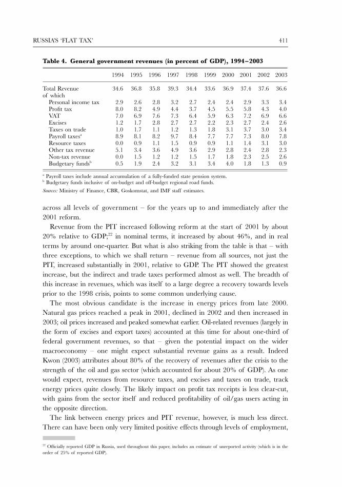
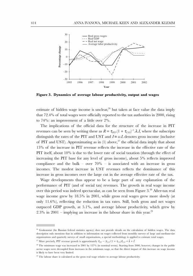
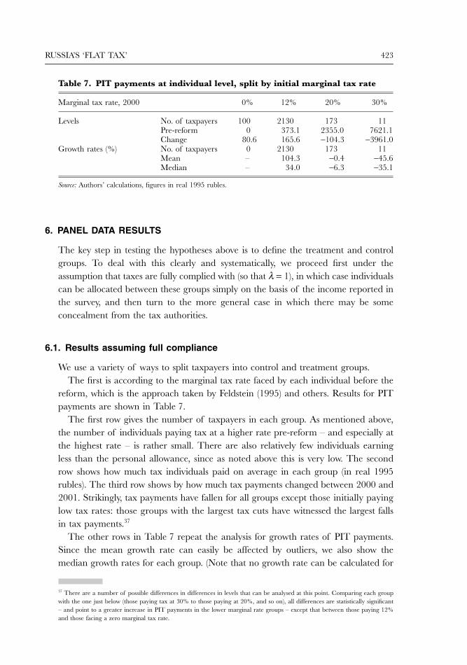
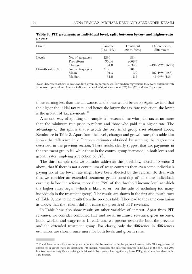
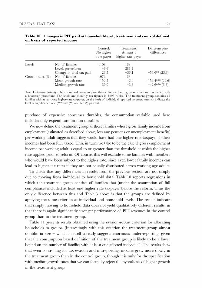
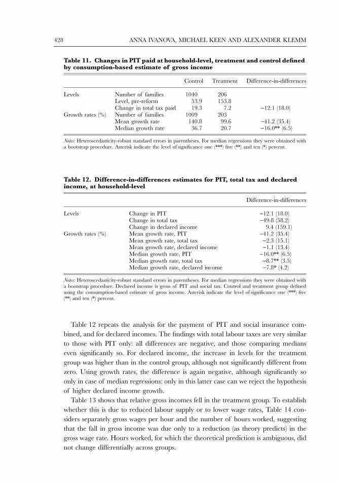
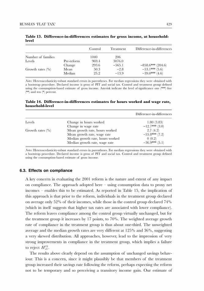
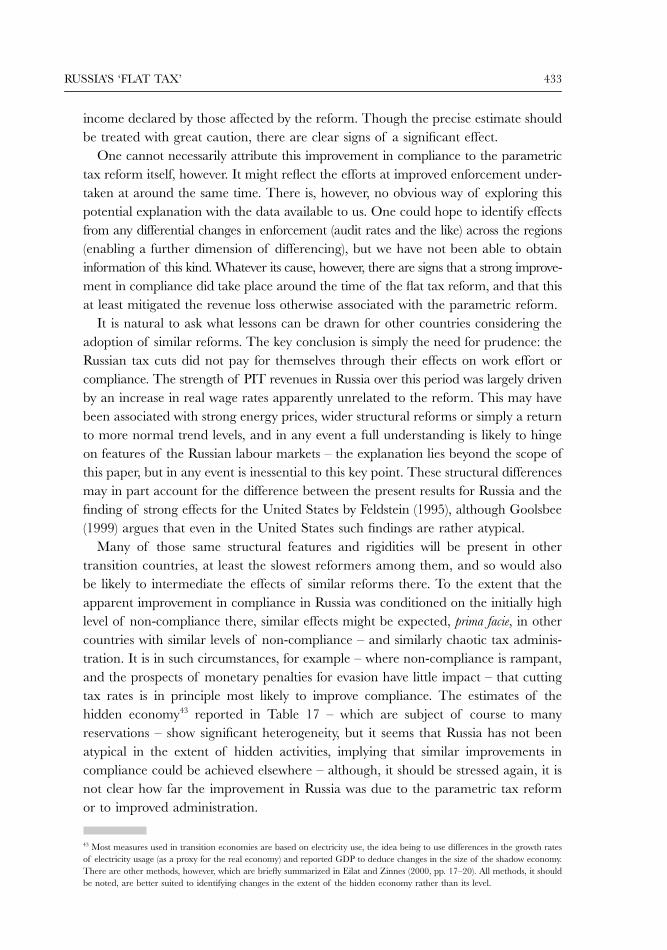
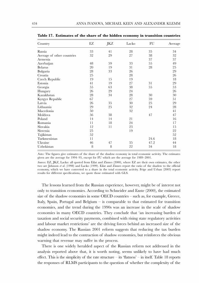
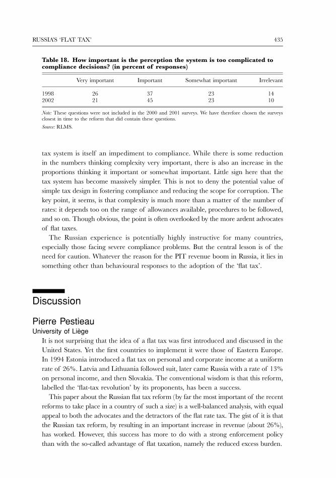
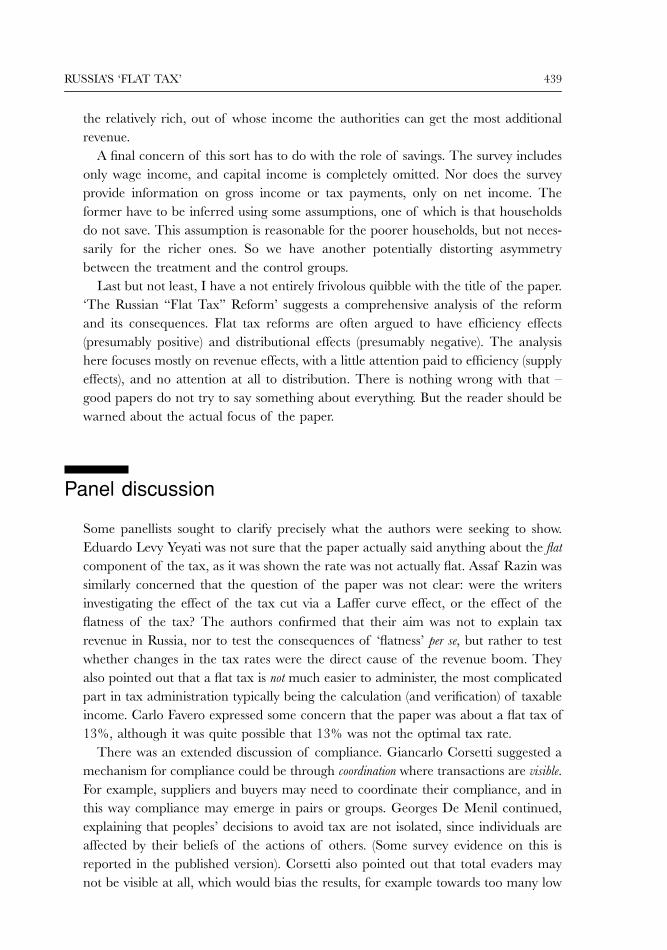Economic Policy July 2005 pp 397ndash444 Printed in Great Britaincopy CEPR CES MSH 2005


Anna Ivanova Michael Keen and Alexander Klemm

International Monetary Fund International Monetary Fund Institute for Fiscal Studies and University College London

1 INTRODUCTION

At the start of 2001 Russia unified its marginal rates of personal income taxation ndashpreviously at 12 20 and 30 ndash at the single rate of 13 In the year following theadoption of this lsquoflat taxrsquo

1

revenue from the personal income tax (PIT) increased byabout 46 (about 26 in real terms) relative to GDP PIT revenues increased bynearly one-fifth Such a strong revenue performance following a marked reduction ofmarginal tax rates quickly attracted attention and emulation in East Europe While theBaltic countries had preceded Russia in introducing single rate income tax structures

2

We thank Richard Blundell Dale Chua Bob Conrad Gohoon Kwon Victoria Perry Ian Preston John Odling Smee NienkeOomes David Owen Pierre Pestieau Carlos Silvani Stephen Smith Antonio Spilimbergo Victor Thuronyi Andreacutes Velascoand participants at the panel meeting for comments and suggestions Opinions expressed here are those of the authors and donot necessarily represent the views or policy of the IMF nor those of the Institute for Fiscal Studies which has no corporateviews At the IFS the work was partially funded by the ESRC Centre for the Microeconomic Analysis of Public Policy

The Managing Editor in charge of this paper was Paul Seabright

1

This term has come to be used extremely loosely The Russian version was not a flat tax in the sense of Hall and Rabushka(1995) which is essentially an expenditure tax implemented by combining a flat tax on wage income and a cash flow businesstax levied at the same rate (although Rabushka (2003) has spoken positively of the Russian experience) More generally thevarious lsquoflat taxesrsquo adopted in Russia and elsewhere differ quite markedly from one another including in whether the rate ofcorporation tax (or even VAT) is aligned with that of the PIT (with the Russian variant in this respect being one of the lessdramatic reforms) Hence the inverted commas in our title

2

Outside Europe Bolivia has had such a tax system since 1986 Other small states and territories (such as Jersey) have had flatrate income taxes for decades



3


4





5


et al

(2003)

6


3


4


The Economist


5


6





7








8


9


10

ndash were taxed at

7

Sinelnikov-Mourylev

et al


8


9


10




11




12


11


12









13

13


+

001

+

0385)(1385) and (013

+

0356)(1356)


Legal incidence



















Value Added Tax



Turnover taxes




14


et al





R

as

τ

λ

wL

where

τ


λ


λ

=


w


L


reg

asymp

3

+

+

w

+

L

(1)


τ


14




31 Gross wage rates


w


15


32 Work effort



16


15


D(w)


S

[

w

(1

minus

λτ


e

D

and

e

S




3

+

lt


16


w

( )=+

minus

+e

e e

S

S D

λτλτ1

3

reg 3 ( )

( )=

minus

+

minus

+

+e e

e e

S D

S D

1

11

λτλτ



a








33 Compliance












34 Income shifting
















1994 1995 1996 1997 1998 1999 2000 2001 2002 2003

















1999 2000 2001 2002


Reported 1408 2126 2826 3749Hidden 526 811 993 1246



















51 Data









52 Methodology























yi = γ0 + γ1Ti + ui (3)




(4)


(5)



H R RLR

T C0 ∆ ∆ge

HLR

0

HLR

0

HGR

T C0 reg regge






(6)







H I ILI

T T C C0λ λ λ ) ( )∆( ∆ge

( )HGI

0λ

HxI0λ

H I ILI

T C0 ∆ ∆ge


H Hxw

xL

0 0 and









I = c + τ (Iλ) (10)

(11)



H HxR

xI

0 0 and λ

λτ λ

( )

( )=

+

minusn Nc I

1




























HxR0






HxR0

HxI0λ

HLI

0λ



20ndash30


Treatment Group


Growth rates ()









(12)



I c Ij jk

k ( )= + sumτ λ









higher rate payer

































HxI0λ










Median 24 358 336 (65)











1998 26 39 21 132002 17 46 25 11


Source RLMS


























Discussion






1998 26 37 23 142002 21 45 23 10


Source RLMS






The Russian reform




Comments

























Panel discussion









DATA APPENDIX

Data sources



RLMS

















Cleaning






4516



3085 (4828)



WEB APPENDIX


REFERENCES
















743 (7791)



2092 (2492)

























3


4





5


et al

(2003)

6


3


4


The Economist


5


6





7








8


9


10

ndash were taxed at

7

Sinelnikov-Mourylev

et al


8


9


10




11




12


11


12









13

13


+

001

+

0385)(1385) and (013

+

0356)(1356)


Legal incidence



















Value Added Tax



Turnover taxes




14


et al





R

as

τ

λ

wL

where

τ


λ


λ

=


w


L


reg

asymp

3

+

+

w

+

L

(1)


τ


14




31 Gross wage rates


w


15


32 Work effort



16


15


D(w)


S

[

w

(1

minus

λτ


e

D

and

e

S




3

+

lt


16


w

( )=+

minus

+e

e e

S

S D

λτλτ1

3

reg 3 ( )

( )=

minus

+

minus

+

+e e

e e

S D

S D

1

11

λτλτ



a








33 Compliance












34 Income shifting
















1994 1995 1996 1997 1998 1999 2000 2001 2002 2003

















1999 2000 2001 2002


Reported 1408 2126 2826 3749Hidden 526 811 993 1246



















51 Data









52 Methodology























yi = γ0 + γ1Ti + ui (3)




(4)


(5)



H R RLR

T C0 ∆ ∆ge

HLR

0

HLR

0

HGR

T C0 reg regge






(6)







H I ILI

T T C C0λ λ λ ) ( )∆( ∆ge

( )HGI

0λ

HxI0λ

H I ILI

T C0 ∆ ∆ge


H Hxw

xL

0 0 and









I = c + τ (Iλ) (10)

(11)



H HxR

xI

0 0 and λ

λτ λ

( )

( )=

+

minusn Nc I

1




























HxR0






HxR0

HxI0λ

HLI

0λ



20ndash30


Treatment Group


Growth rates ()









(12)



I c Ij jk

k ( )= + sumτ λ









higher rate payer

































HxI0λ










Median 24 358 336 (65)











1998 26 39 21 132002 17 46 25 11


Source RLMS


























Discussion






1998 26 37 23 142002 21 45 23 10


Source RLMS






The Russian reform




Comments

























Panel discussion









DATA APPENDIX

Data sources



RLMS

















Cleaning






4516



3085 (4828)



WEB APPENDIX


REFERENCES
















743 (7791)



2092 (2492)


























7








8


9


10

ndash were taxed at

7

Sinelnikov-Mourylev

et al


8


9


10




11




12


11


12









13

13


+

001

+

0385)(1385) and (013

+

0356)(1356)


Legal incidence



















Value Added Tax



Turnover taxes




14


et al





R

as

τ

λ

wL

where

τ


λ


λ

=


w


L


reg

asymp

3

+

+

w

+

L

(1)


τ


14




31 Gross wage rates


w


15


32 Work effort



16


15


D(w)


S

[

w

(1

minus

λτ


e

D

and

e

S




3

+

lt


16


w

( )=+

minus

+e

e e

S

S D

λτλτ1

3

reg 3 ( )

( )=

minus

+

minus

+

+e e

e e

S D

S D

1

11

λτλτ



a








33 Compliance












34 Income shifting
















1994 1995 1996 1997 1998 1999 2000 2001 2002 2003

















1999 2000 2001 2002


Reported 1408 2126 2826 3749Hidden 526 811 993 1246



















51 Data









52 Methodology























yi = γ0 + γ1Ti + ui (3)




(4)


(5)



H R RLR

T C0 ∆ ∆ge

HLR

0

HLR

0

HGR

T C0 reg regge






(6)







H I ILI

T T C C0λ λ λ ) ( )∆( ∆ge

( )HGI

0λ

HxI0λ

H I ILI

T C0 ∆ ∆ge


H Hxw

xL

0 0 and









I = c + τ (Iλ) (10)

(11)



H HxR

xI

0 0 and λ

λτ λ

( )

( )=

+

minusn Nc I

1




























HxR0






HxR0

HxI0λ

HLI

0λ



20ndash30


Treatment Group


Growth rates ()









(12)



I c Ij jk

k ( )= + sumτ λ









higher rate payer

































HxI0λ










Median 24 358 336 (65)











1998 26 39 21 132002 17 46 25 11


Source RLMS


























Discussion






1998 26 37 23 142002 21 45 23 10


Source RLMS






The Russian reform




Comments

























Panel discussion









DATA APPENDIX

Data sources



RLMS

















Cleaning






4516



3085 (4828)



WEB APPENDIX


REFERENCES
















743 (7791)



2092 (2492)

























11




12


11


12









13

13


+

001

+

0385)(1385) and (013

+

0356)(1356)


Legal incidence



















Value Added Tax



Turnover taxes




14


et al





R

as

τ

λ

wL

where

τ


λ


λ

=


w


L


reg

asymp

3

+

+

w

+

L

(1)


τ


14




31 Gross wage rates


w


15


32 Work effort



16


15


D(w)


S

[

w

(1

minus

λτ


e

D

and

e

S




3

+

lt


16


w

( )=+

minus

+e

e e

S

S D

λτλτ1

3

reg 3 ( )

( )=

minus

+

minus

+

+e e

e e

S D

S D

1

11

λτλτ



a








33 Compliance












34 Income shifting
















1994 1995 1996 1997 1998 1999 2000 2001 2002 2003

















1999 2000 2001 2002


Reported 1408 2126 2826 3749Hidden 526 811 993 1246



















51 Data









52 Methodology























yi = γ0 + γ1Ti + ui (3)




(4)


(5)



H R RLR

T C0 ∆ ∆ge

HLR

0

HLR

0

HGR

T C0 reg regge






(6)







H I ILI

T T C C0λ λ λ ) ( )∆( ∆ge

( )HGI

0λ

HxI0λ

H I ILI

T C0 ∆ ∆ge


H Hxw

xL

0 0 and









I = c + τ (Iλ) (10)

(11)



H HxR

xI

0 0 and λ

λτ λ

( )

( )=

+

minusn Nc I

1




























HxR0






HxR0

HxI0λ

HLI

0λ



20ndash30


Treatment Group


Growth rates ()









(12)



I c Ij jk

k ( )= + sumτ λ









higher rate payer

































HxI0λ










Median 24 358 336 (65)











1998 26 39 21 132002 17 46 25 11


Source RLMS


























Discussion






1998 26 37 23 142002 21 45 23 10


Source RLMS






The Russian reform




Comments

























Panel discussion









DATA APPENDIX

Data sources



RLMS

















Cleaning






4516



3085 (4828)



WEB APPENDIX


REFERENCES
















743 (7791)



2092 (2492)

























13

13


+

001

+

0385)(1385) and (013

+

0356)(1356)


Legal incidence



















Value Added Tax



Turnover taxes




14


et al





R

as

τ

λ

wL

where

τ


λ


λ

=


w


L


reg

asymp

3

+

+

w

+

L

(1)


τ


14




31 Gross wage rates


w


15


32 Work effort



16


15


D(w)


S

[

w

(1

minus

λτ


e

D

and

e

S




3

+

lt


16


w

( )=+

minus

+e

e e

S

S D

λτλτ1

3

reg 3 ( )

( )=

minus

+

minus

+

+e e

e e

S D

S D

1

11

λτλτ



a








33 Compliance












34 Income shifting
















1994 1995 1996 1997 1998 1999 2000 2001 2002 2003

















1999 2000 2001 2002


Reported 1408 2126 2826 3749Hidden 526 811 993 1246



















51 Data









52 Methodology























yi = γ0 + γ1Ti + ui (3)




(4)


(5)



H R RLR

T C0 ∆ ∆ge

HLR

0

HLR

0

HGR

T C0 reg regge






(6)







H I ILI

T T C C0λ λ λ ) ( )∆( ∆ge

( )HGI

0λ

HxI0λ

H I ILI

T C0 ∆ ∆ge


H Hxw

xL

0 0 and









I = c + τ (Iλ) (10)

(11)



H HxR

xI

0 0 and λ

λτ λ

( )

( )=

+

minusn Nc I

1




























HxR0






HxR0

HxI0λ

HLI

0λ



20ndash30


Treatment Group


Growth rates ()









(12)



I c Ij jk

k ( )= + sumτ λ









higher rate payer

































HxI0λ










Median 24 358 336 (65)











1998 26 39 21 132002 17 46 25 11


Source RLMS


























Discussion






1998 26 37 23 142002 21 45 23 10


Source RLMS






The Russian reform




Comments

























Panel discussion









DATA APPENDIX

Data sources



RLMS

















Cleaning






4516



3085 (4828)



WEB APPENDIX


REFERENCES
















743 (7791)



2092 (2492)

































Value Added Tax



Turnover taxes




14


et al





R

as

τ

λ

wL

where

τ


λ


λ

=


w


L


reg

asymp

3

+

+

w

+

L

(1)


τ


14




31 Gross wage rates


w


15


32 Work effort



16


15


D(w)


S

[

w

(1

minus

λτ


e

D

and

e

S




3

+

lt


16


w

( )=+

minus

+e

e e

S

S D

λτλτ1

3

reg 3 ( )

( )=

minus

+

minus

+

+e e

e e

S D

S D

1

11

λτλτ



a








33 Compliance












34 Income shifting
















1994 1995 1996 1997 1998 1999 2000 2001 2002 2003

















1999 2000 2001 2002


Reported 1408 2126 2826 3749Hidden 526 811 993 1246



















51 Data









52 Methodology























yi = γ0 + γ1Ti + ui (3)




(4)


(5)



H R RLR

T C0 ∆ ∆ge

HLR

0

HLR

0

HGR

T C0 reg regge






(6)







H I ILI

T T C C0λ λ λ ) ( )∆( ∆ge

( )HGI

0λ

HxI0λ

H I ILI

T C0 ∆ ∆ge


H Hxw

xL

0 0 and









I = c + τ (Iλ) (10)

(11)



H HxR

xI

0 0 and λ

λτ λ

( )

( )=

+

minusn Nc I

1




























HxR0






HxR0

HxI0λ

HLI

0λ



20ndash30


Treatment Group


Growth rates ()









(12)



I c Ij jk

k ( )= + sumτ λ









higher rate payer

































HxI0λ










Median 24 358 336 (65)











1998 26 39 21 132002 17 46 25 11


Source RLMS


























Discussion






1998 26 37 23 142002 21 45 23 10


Source RLMS






The Russian reform




Comments

























Panel discussion









DATA APPENDIX

Data sources



RLMS

















Cleaning






4516



3085 (4828)



WEB APPENDIX


REFERENCES
















743 (7791)



2092 (2492)

























14


et al





R

as

τ

λ

wL

where

τ


λ


λ

=


w


L


reg

asymp

3

+

+

w

+

L

(1)


τ


14




31 Gross wage rates


w


15


32 Work effort



16


15


D(w)


S

[

w

(1

minus

λτ


e

D

and

e

S




3

+

lt


16


w

( )=+

minus

+e

e e

S

S D

λτλτ1

3

reg 3 ( )

( )=

minus

+

minus

+

+e e

e e

S D

S D

1

11

λτλτ



a








33 Compliance












34 Income shifting
















1994 1995 1996 1997 1998 1999 2000 2001 2002 2003

















1999 2000 2001 2002


Reported 1408 2126 2826 3749Hidden 526 811 993 1246



















51 Data









52 Methodology























yi = γ0 + γ1Ti + ui (3)




(4)


(5)



H R RLR

T C0 ∆ ∆ge

HLR

0

HLR

0

HGR

T C0 reg regge






(6)







H I ILI

T T C C0λ λ λ ) ( )∆( ∆ge

( )HGI

0λ

HxI0λ

H I ILI

T C0 ∆ ∆ge


H Hxw

xL

0 0 and









I = c + τ (Iλ) (10)

(11)



H HxR

xI

0 0 and λ

λτ λ

( )

( )=

+

minusn Nc I

1




























HxR0






HxR0

HxI0λ

HLI

0λ



20ndash30


Treatment Group


Growth rates ()









(12)



I c Ij jk

k ( )= + sumτ λ









higher rate payer

































HxI0λ










Median 24 358 336 (65)











1998 26 39 21 132002 17 46 25 11


Source RLMS


























Discussion






1998 26 37 23 142002 21 45 23 10


Source RLMS






The Russian reform




Comments

























Panel discussion









DATA APPENDIX

Data sources



RLMS

















Cleaning






4516



3085 (4828)



WEB APPENDIX


REFERENCES
















743 (7791)



2092 (2492)

























31 Gross wage rates


w


15


32 Work effort



16


15


D(w)


S

[

w

(1

minus

λτ


e

D

and

e

S




3

+

lt


16


w

( )=+

minus

+e

e e

S

S D

λτλτ1

3

reg 3 ( )

( )=

minus

+

minus

+

+e e

e e

S D

S D

1

11

λτλτ



a








33 Compliance












34 Income shifting
















1994 1995 1996 1997 1998 1999 2000 2001 2002 2003

















1999 2000 2001 2002


Reported 1408 2126 2826 3749Hidden 526 811 993 1246



















51 Data









52 Methodology























yi = γ0 + γ1Ti + ui (3)




(4)


(5)



H R RLR

T C0 ∆ ∆ge

HLR

0

HLR

0

HGR

T C0 reg regge






(6)







H I ILI

T T C C0λ λ λ ) ( )∆( ∆ge

( )HGI

0λ

HxI0λ

H I ILI

T C0 ∆ ∆ge


H Hxw

xL

0 0 and









I = c + τ (Iλ) (10)

(11)



H HxR

xI

0 0 and λ

λτ λ

( )

( )=

+

minusn Nc I

1




























HxR0






HxR0

HxI0λ

HLI

0λ



20ndash30


Treatment Group


Growth rates ()









(12)



I c Ij jk

k ( )= + sumτ λ









higher rate payer

































HxI0λ










Median 24 358 336 (65)











1998 26 39 21 132002 17 46 25 11


Source RLMS


























Discussion






1998 26 37 23 142002 21 45 23 10


Source RLMS






The Russian reform




Comments

























Panel discussion









DATA APPENDIX

Data sources



RLMS

















Cleaning






4516



3085 (4828)



WEB APPENDIX


REFERENCES
















743 (7791)



2092 (2492)

























a








33 Compliance












34 Income shifting
















1994 1995 1996 1997 1998 1999 2000 2001 2002 2003

















1999 2000 2001 2002


Reported 1408 2126 2826 3749Hidden 526 811 993 1246



















51 Data









52 Methodology























yi = γ0 + γ1Ti + ui (3)




(4)


(5)



H R RLR

T C0 ∆ ∆ge

HLR

0

HLR

0

HGR

T C0 reg regge






(6)







H I ILI

T T C C0λ λ λ ) ( )∆( ∆ge

( )HGI

0λ

HxI0λ

H I ILI

T C0 ∆ ∆ge


H Hxw

xL

0 0 and









I = c + τ (Iλ) (10)

(11)



H HxR

xI

0 0 and λ

λτ λ

( )

( )=

+

minusn Nc I

1




























HxR0






HxR0

HxI0λ

HLI

0λ



20ndash30


Treatment Group


Growth rates ()









(12)



I c Ij jk

k ( )= + sumτ λ









higher rate payer

































HxI0λ










Median 24 358 336 (65)











1998 26 39 21 132002 17 46 25 11


Source RLMS


























Discussion






1998 26 37 23 142002 21 45 23 10


Source RLMS






The Russian reform




Comments

























Panel discussion









DATA APPENDIX

Data sources



RLMS

















Cleaning






4516



3085 (4828)



WEB APPENDIX


REFERENCES
















743 (7791)



2092 (2492)


























33 Compliance












34 Income shifting
















1994 1995 1996 1997 1998 1999 2000 2001 2002 2003

















1999 2000 2001 2002


Reported 1408 2126 2826 3749Hidden 526 811 993 1246



















51 Data









52 Methodology























yi = γ0 + γ1Ti + ui (3)




(4)


(5)



H R RLR

T C0 ∆ ∆ge

HLR

0

HLR

0

HGR

T C0 reg regge






(6)







H I ILI

T T C C0λ λ λ ) ( )∆( ∆ge

( )HGI

0λ

HxI0λ

H I ILI

T C0 ∆ ∆ge


H Hxw

xL

0 0 and









I = c + τ (Iλ) (10)

(11)



H HxR

xI

0 0 and λ

λτ λ

( )

( )=

+

minusn Nc I

1




























HxR0






HxR0

HxI0λ

HLI

0λ



20ndash30


Treatment Group


Growth rates ()









(12)



I c Ij jk

k ( )= + sumτ λ









higher rate payer

































HxI0λ










Median 24 358 336 (65)











1998 26 39 21 132002 17 46 25 11


Source RLMS


























Discussion






1998 26 37 23 142002 21 45 23 10


Source RLMS






The Russian reform




Comments

























Panel discussion









DATA APPENDIX

Data sources



RLMS

















Cleaning






4516



3085 (4828)



WEB APPENDIX


REFERENCES
















743 (7791)



2092 (2492)































34 Income shifting
















1994 1995 1996 1997 1998 1999 2000 2001 2002 2003

















1999 2000 2001 2002


Reported 1408 2126 2826 3749Hidden 526 811 993 1246



















51 Data









52 Methodology























yi = γ0 + γ1Ti + ui (3)




(4)


(5)



H R RLR

T C0 ∆ ∆ge

HLR

0

HLR

0

HGR

T C0 reg regge






(6)







H I ILI

T T C C0λ λ λ ) ( )∆( ∆ge

( )HGI

0λ

HxI0λ

H I ILI

T C0 ∆ ∆ge


H Hxw

xL

0 0 and









I = c + τ (Iλ) (10)

(11)



H HxR

xI

0 0 and λ

λτ λ

( )

( )=

+

minusn Nc I

1




























HxR0






HxR0

HxI0λ

HLI

0λ



20ndash30


Treatment Group


Growth rates ()









(12)



I c Ij jk

k ( )= + sumτ λ









higher rate payer

































HxI0λ










Median 24 358 336 (65)











1998 26 39 21 132002 17 46 25 11


Source RLMS


























Discussion






1998 26 37 23 142002 21 45 23 10


Source RLMS






The Russian reform




Comments

























Panel discussion









DATA APPENDIX

Data sources



RLMS

















Cleaning






4516



3085 (4828)



WEB APPENDIX


REFERENCES
















743 (7791)



2092 (2492)






























1994 1995 1996 1997 1998 1999 2000 2001 2002 2003

















1999 2000 2001 2002


Reported 1408 2126 2826 3749Hidden 526 811 993 1246



















51 Data









52 Methodology























yi = γ0 + γ1Ti + ui (3)




(4)


(5)



H R RLR

T C0 ∆ ∆ge

HLR

0

HLR

0

HGR

T C0 reg regge






(6)







H I ILI

T T C C0λ λ λ ) ( )∆( ∆ge

( )HGI

0λ

HxI0λ

H I ILI

T C0 ∆ ∆ge


H Hxw

xL

0 0 and









I = c + τ (Iλ) (10)

(11)



H HxR

xI

0 0 and λ

λτ λ

( )

( )=

+

minusn Nc I

1




























HxR0






HxR0

HxI0λ

HLI

0λ



20ndash30


Treatment Group


Growth rates ()









(12)



I c Ij jk

k ( )= + sumτ λ









higher rate payer

































HxI0λ










Median 24 358 336 (65)











1998 26 39 21 132002 17 46 25 11


Source RLMS


























Discussion






1998 26 37 23 142002 21 45 23 10


Source RLMS






The Russian reform




Comments

























Panel discussion









DATA APPENDIX

Data sources



RLMS

















Cleaning






4516



3085 (4828)



WEB APPENDIX


REFERENCES
















743 (7791)



2092 (2492)



































1999 2000 2001 2002


Reported 1408 2126 2826 3749Hidden 526 811 993 1246



















51 Data









52 Methodology























yi = γ0 + γ1Ti + ui (3)




(4)


(5)



H R RLR

T C0 ∆ ∆ge

HLR

0

HLR

0

HGR

T C0 reg regge






(6)







H I ILI

T T C C0λ λ λ ) ( )∆( ∆ge

( )HGI

0λ

HxI0λ

H I ILI

T C0 ∆ ∆ge


H Hxw

xL

0 0 and









I = c + τ (Iλ) (10)

(11)



H HxR

xI

0 0 and λ

λτ λ

( )

( )=

+

minusn Nc I

1




























HxR0






HxR0

HxI0λ

HLI

0λ



20ndash30


Treatment Group


Growth rates ()









(12)



I c Ij jk

k ( )= + sumτ λ









higher rate payer

































HxI0λ










Median 24 358 336 (65)











1998 26 39 21 132002 17 46 25 11


Source RLMS


























Discussion






1998 26 37 23 142002 21 45 23 10


Source RLMS






The Russian reform




Comments

























Panel discussion









DATA APPENDIX

Data sources



RLMS

















Cleaning






4516



3085 (4828)



WEB APPENDIX


REFERENCES
















743 (7791)



2092 (2492)





































51 Data









52 Methodology























yi = γ0 + γ1Ti + ui (3)




(4)


(5)



H R RLR

T C0 ∆ ∆ge

HLR

0

HLR

0

HGR

T C0 reg regge






(6)







H I ILI

T T C C0λ λ λ ) ( )∆( ∆ge

( )HGI

0λ

HxI0λ

H I ILI

T C0 ∆ ∆ge


H Hxw

xL

0 0 and









I = c + τ (Iλ) (10)

(11)



H HxR

xI

0 0 and λ

λτ λ

( )

( )=

+

minusn Nc I

1




























HxR0






HxR0

HxI0λ

HLI

0λ



20ndash30


Treatment Group


Growth rates ()









(12)



I c Ij jk

k ( )= + sumτ λ









higher rate payer

































HxI0λ










Median 24 358 336 (65)











1998 26 39 21 132002 17 46 25 11


Source RLMS


























Discussion






1998 26 37 23 142002 21 45 23 10


Source RLMS






The Russian reform




Comments

























Panel discussion









DATA APPENDIX

Data sources



RLMS

















Cleaning






4516



3085 (4828)



WEB APPENDIX


REFERENCES
















743 (7791)



2092 (2492)



























52 Methodology























yi = γ0 + γ1Ti + ui (3)




(4)


(5)



H R RLR

T C0 ∆ ∆ge

HLR

0

HLR

0

HGR

T C0 reg regge






(6)







H I ILI

T T C C0λ λ λ ) ( )∆( ∆ge

( )HGI

0λ

HxI0λ

H I ILI

T C0 ∆ ∆ge


H Hxw

xL

0 0 and









I = c + τ (Iλ) (10)

(11)



H HxR

xI

0 0 and λ

λτ λ

( )

( )=

+

minusn Nc I

1




























HxR0






HxR0

HxI0λ

HLI

0λ



20ndash30


Treatment Group


Growth rates ()









(12)



I c Ij jk

k ( )= + sumτ λ









higher rate payer

































HxI0λ










Median 24 358 336 (65)











1998 26 39 21 132002 17 46 25 11


Source RLMS


























Discussion






1998 26 37 23 142002 21 45 23 10


Source RLMS






The Russian reform




Comments

























Panel discussion









DATA APPENDIX

Data sources



RLMS

















Cleaning






4516



3085 (4828)



WEB APPENDIX


REFERENCES
















743 (7791)



2092 (2492)







































yi = γ0 + γ1Ti + ui (3)




(4)


(5)



H R RLR

T C0 ∆ ∆ge

HLR

0

HLR

0

HGR

T C0 reg regge






(6)







H I ILI

T T C C0λ λ λ ) ( )∆( ∆ge

( )HGI

0λ

HxI0λ

H I ILI

T C0 ∆ ∆ge


H Hxw

xL

0 0 and









I = c + τ (Iλ) (10)

(11)



H HxR

xI

0 0 and λ

λτ λ

( )

( )=

+

minusn Nc I

1




























HxR0






HxR0

HxI0λ

HLI

0λ



20ndash30


Treatment Group


Growth rates ()









(12)



I c Ij jk

k ( )= + sumτ λ









higher rate payer

































HxI0λ










Median 24 358 336 (65)











1998 26 39 21 132002 17 46 25 11


Source RLMS


























Discussion






1998 26 37 23 142002 21 45 23 10


Source RLMS






The Russian reform




Comments

























Panel discussion









DATA APPENDIX

Data sources



RLMS

















Cleaning






4516



3085 (4828)



WEB APPENDIX


REFERENCES
















743 (7791)



2092 (2492)




























(6)







H I ILI

T T C C0λ λ λ ) ( )∆( ∆ge

( )HGI

0λ

HxI0λ

H I ILI

T C0 ∆ ∆ge


H Hxw

xL

0 0 and









I = c + τ (Iλ) (10)

(11)



H HxR

xI

0 0 and λ

λτ λ

( )

( )=

+

minusn Nc I

1




























HxR0






HxR0

HxI0λ

HLI

0λ



20ndash30


Treatment Group


Growth rates ()









(12)



I c Ij jk

k ( )= + sumτ λ









higher rate payer

































HxI0λ










Median 24 358 336 (65)











1998 26 39 21 132002 17 46 25 11


Source RLMS


























Discussion






1998 26 37 23 142002 21 45 23 10


Source RLMS






The Russian reform




Comments

























Panel discussion









DATA APPENDIX

Data sources



RLMS

















Cleaning






4516



3085 (4828)



WEB APPENDIX


REFERENCES
















743 (7791)



2092 (2492)































I = c + τ (Iλ) (10)

(11)



H HxR

xI

0 0 and λ

λτ λ

( )

( )=

+

minusn Nc I

1




























HxR0






HxR0

HxI0λ

HLI

0λ



20ndash30


Treatment Group


Growth rates ()









(12)



I c Ij jk

k ( )= + sumτ λ









higher rate payer

































HxI0λ










Median 24 358 336 (65)











1998 26 39 21 132002 17 46 25 11


Source RLMS


























Discussion






1998 26 37 23 142002 21 45 23 10


Source RLMS






The Russian reform




Comments

























Panel discussion









DATA APPENDIX

Data sources



RLMS

















Cleaning






4516



3085 (4828)



WEB APPENDIX


REFERENCES
















743 (7791)



2092 (2492)


















































HxR0






HxR0

HxI0λ

HLI

0λ



20ndash30


Treatment Group


Growth rates ()









(12)



I c Ij jk

k ( )= + sumτ λ









higher rate payer

































HxI0λ










Median 24 358 336 (65)











1998 26 39 21 132002 17 46 25 11


Source RLMS


























Discussion






1998 26 37 23 142002 21 45 23 10


Source RLMS






The Russian reform




Comments

























Panel discussion









DATA APPENDIX

Data sources



RLMS

















Cleaning






4516



3085 (4828)



WEB APPENDIX


REFERENCES
















743 (7791)



2092 (2492)




























HxR0

HxI0λ

HLI

0λ



20ndash30


Treatment Group


Growth rates ()









(12)



I c Ij jk

k ( )= + sumτ λ









higher rate payer

































HxI0λ










Median 24 358 336 (65)











1998 26 39 21 132002 17 46 25 11


Source RLMS


























Discussion






1998 26 37 23 142002 21 45 23 10


Source RLMS






The Russian reform




Comments

























Panel discussion









DATA APPENDIX

Data sources



RLMS

















Cleaning






4516



3085 (4828)



WEB APPENDIX


REFERENCES
















743 (7791)



2092 (2492)





























(12)



I c Ij jk

k ( )= + sumτ λ









higher rate payer

































HxI0λ










Median 24 358 336 (65)











1998 26 39 21 132002 17 46 25 11


Source RLMS


























Discussion






1998 26 37 23 142002 21 45 23 10


Source RLMS






The Russian reform




Comments

























Panel discussion









DATA APPENDIX

Data sources



RLMS

















Cleaning






4516



3085 (4828)



WEB APPENDIX


REFERENCES
















743 (7791)



2092 (2492)































higher rate payer

































HxI0λ










Median 24 358 336 (65)











1998 26 39 21 132002 17 46 25 11


Source RLMS


























Discussion






1998 26 37 23 142002 21 45 23 10


Source RLMS






The Russian reform




Comments

























Panel discussion









DATA APPENDIX

Data sources



RLMS

















Cleaning






4516



3085 (4828)



WEB APPENDIX


REFERENCES
















743 (7791)



2092 (2492)



















































HxI0λ










Median 24 358 336 (65)











1998 26 39 21 132002 17 46 25 11


Source RLMS


























Discussion






1998 26 37 23 142002 21 45 23 10


Source RLMS






The Russian reform




Comments

























Panel discussion









DATA APPENDIX

Data sources



RLMS

















Cleaning






4516



3085 (4828)



WEB APPENDIX


REFERENCES
















743 (7791)



2092 (2492)
































Median 24 358 336 (65)











1998 26 39 21 132002 17 46 25 11


Source RLMS


























Discussion






1998 26 37 23 142002 21 45 23 10


Source RLMS






The Russian reform




Comments

























Panel discussion









DATA APPENDIX

Data sources



RLMS

















Cleaning






4516



3085 (4828)



WEB APPENDIX


REFERENCES
















743 (7791)



2092 (2492)
































1998 26 39 21 132002 17 46 25 11


Source RLMS


























Discussion






1998 26 37 23 142002 21 45 23 10


Source RLMS






The Russian reform




Comments

























Panel discussion









DATA APPENDIX

Data sources



RLMS

















Cleaning






4516



3085 (4828)



WEB APPENDIX


REFERENCES
















743 (7791)



2092 (2492)
















































Discussion






1998 26 37 23 142002 21 45 23 10


Source RLMS






The Russian reform




Comments

























Panel discussion









DATA APPENDIX

Data sources



RLMS

















Cleaning






4516



3085 (4828)



WEB APPENDIX


REFERENCES
















743 (7791)



2092 (2492)




























The Russian reform




Comments

























Panel discussion









DATA APPENDIX

Data sources



RLMS

















Cleaning






4516



3085 (4828)



WEB APPENDIX


REFERENCES
















743 (7791)



2092 (2492)














































Panel discussion









DATA APPENDIX

Data sources



RLMS

















Cleaning






4516



3085 (4828)



WEB APPENDIX


REFERENCES
















743 (7791)



2092 (2492)





























DATA APPENDIX

Data sources



RLMS

















Cleaning






4516



3085 (4828)



WEB APPENDIX


REFERENCES
















743 (7791)



2092 (2492)
























RLMS

















Cleaning






4516



3085 (4828)



WEB APPENDIX


REFERENCES
















743 (7791)



2092 (2492)


























Cleaning






4516



3085 (4828)



WEB APPENDIX


REFERENCES
















743 (7791)



2092 (2492)

























WEB APPENDIX


REFERENCES
















743 (7791)



2092 (2492)





















