Taxation and International Migration of Superstars:Evidence from the European Football Market∗

Henrik Jacobsen Kleven, London School of Economics

Camille Landais, Stanford University

Emmanuel Saez, UC Berkeley

February 2011

Abstract

This paper analyzes the effects of top earnings tax rates on the international migra-tion of top football players in Europe. We construct a panel data set of top earnings taxrates, football player careers, and club performances in the first leagues of 14 Europeancountries since 1985. We identify the effects of top earnings tax rates on migration using anumber of tax and institutional changes: (a) the 1995 Bosman ruling which liberalized theEuropean football market, (b) top tax rate reforms within countries, and (c) special taxschemes offering preferential tax rates to immigrant football players. We start by present-ing reduced-form graphical evidence showing large and compelling migration responses tocountry-specific tax reforms and labor market regulation. We then set out a theoreticalmodel of taxation and migration, which is tested using all sources of tax variation simul-taneously. Our results show that (i) the overall location elasticity with respect to thenet-of-tax rate is positive and large, (ii) location elasticities are extremely large at the topof the ability distribution but negative at the bottom due to ability sorting effects, and(iii) cross-tax effects of foreign players on domestic players (and vice versa) are negativeand quite strong due to displacement effects. Finally, we estimate tax revenue maximizingrates and draw policy conclusions.

∗We would like to thank Raj Chetty, Caroline Hoxby, Larry Katz, Wojciech Kopczuk, Claus Kreiner, ThomasPiketty, James Poterba, Guttorm Schjelderup, Dan Silverman, Joel Slemrod, and numerous seminar participantsfor helpful comments and discussions. We are also grateful to Filip Rozsypal and Ben Eisenpress for outstandingresearch assistance. Financial support from the Center for Equitable Growth at UC Berkeley, the European TaxPolicy Forum, and NSF Grant SES-0850631 is gratefully acknowledged.

1 Introduction

Tax-induced international mobility of talent is a crucial public policy issue, especially when

tax rates differ substantially across countries and migration barriers are low as in the case

of the European Union. In this case, high tax rates on high-paid workers may induce such

workers to migrate to countries where the tax burden is lower. Therefore, international mobility

may severely limit the ability of governments to redistribute income through highly progressive

taxation. A theoretical literature, following on the seminal contribution by Mirrlees (1982),

has analyzed optimal taxation in the presence of international migration (e.g., Bhagwati and

Wilson, 1989; Cremer et al., 1996; Wildasin, 1998). In particular, concerns have been raised

that the mobility of skilled workers is generating harmful tax competition driving down the

progressivity of taxation in European countries.1 As a result, the mobility response to high

tax rates perhaps looms even larger in the policy debate on optimal tax progressivity than

traditional within-country labor supply responses.

While an enormous empirical literature has studied labor supply and taxable income re-

sponses to taxation (as surveyed by, e.g., Blundell and MaCurdy 1999, Slemrod 1998, and Saez,

Slemrod and Giertz 2011), there is very little empirical work on the effect of taxation on the

spatial mobility of people, and especially mobility among high-skilled workers. A small litera-

ture has considered the mobility of people across local jurisdictions within countries, including

Kirchgassner and Pommerehne (1996) and Liebig et al. (2007) on mobility across Swiss Cantons

in response to Canton taxes, Feldstein and Wrobel (1998) and Bakija and Slemrod (2004) on

mobility across U.S. states in response to state income taxes, and Meyer (2000) on mobility

across U.S. states in response to state welfare programs. However, empirical work on the effect

of taxation on international mobility appears to be virtually non-existent.2 The reason for this

is a lack of micro data containing citizenship information along with issues about how to identify

causal effects on migration. This paper takes a first step to fill this gap in the literature by

1There is a large theoretical literature on tax competition studying strategic tax setting across countries inorder to attract mobile production factors. Most of this literature has focused on capital income taxation (e.g.,Wilson, 1999), but some of it has analyzed labor income taxation with internationally mobile labor (e.g., Wilson,1995 and Wildasin, 2006).

2There is a very large literature on the effects of capital taxation on multinational corporations and inter-national capital mobility (surveyed by, e.g., Gordon and Hines, 2002). There is also an enormous literatureon wage differentials and international migration (see e.g., Borjas, 1999 for a survey). and some work on howinternational migration is affected by the generosity of social insurance and social welfare programs (see e.g.,Borjas, 1999).

1

focusing on the specific labor market for professional football players in Europe.

The European football market offers four important advantages for the study of mobility and

taxation. First, professional football is a small but highly visible segment of the high-skilled

labor market as a large fraction of the European population follows the sport closely. As a

result, tax-induced mobility of football players is of interest in its own right. Indeed, this topic

has recently been the subject of heated discussion in the UK in connection with the increase in

the top marginal tax rate from 40% to 50%. Supposedly, the star player Christiano Ronaldo

moved from Manchester United to Real Madrid in 2009 in part to avoid the announced 50% tax

in the U.K. and instead benefit from the so-called “Beckham Law” in Spain offering a flat tax of

24% to foreign residents.3 Arsene Wenger, the emblematic manager of Arsenal FC, commented

on the UK tax reform by saying that “with the new taxation system,..., the domination of the

Premier League will go, that is for sure” (The Sunday Times, April 25, 2009).4

Second, international mobility is relatively common in the professional football market,

making it a valuable laboratory to begin the study of tax-induced mobility across countries.

This market has a relatively high degree of cross-border mobility because the profession involves

very little country-specific human capital as the game is the same everywhere. We therefore

see this study as providing an upper bound on the migration response to taxation for the labor

market as a whole. Obtaining an upper bound is crucial to gauge the potential importance of

this policy question, especially in the long run as labor markets become more international and

country-specific human capital declines in importance.

Third and crucially, extensive data on the careers and mobility of professional football players

can be gathered for most countries over long time periods. For this project, we have gathered

exhaustive data on the career paths of all first-league football players (top 20 or so football teams

in each country) for 14 European countries over the past 30 years, as well as performance data

for all first-league teams. We have also collected top earnings tax rate data across countries and

over time, taking into account special tax rules applying to immigrant workers and sometimes

to athletes specifically. As top football players earn very high salaries, their average tax rate is

3Although the tax increase in the UK did not take effect until April 2010, the tax reform was passed inparliament in April 2009, several months prior to Ronaldo signing the contract with Real Madrid. The “BeckhamLaw” refers to a preferential tax scheme for foreign residents in Spain. The scheme was introduced in 2005, andgot its nickname after the superstar player David Beckham became one of the first foreigners to benefit fromthe scheme when he moved from Manchester United to Real Madrid.

4In the United States, the mobility of Baseball stars across states for tax reasons is also debated. Ross andDunn (2007) show that the salaries of baseball players adjust to offset the burden of state income taxes.

2

well approximated by the top marginal tax rate applying to earnings when combining (a) the

top statutory individual income tax rate, (b) social security contributions (of both employees

and employers) when such taxes apply to uncapped earnings, and (c) value-added taxes.

Fourth, there are many sources of variation in both tax policy and labor market regulation,

which can be exploited to identify the effect of taxation on mobility in the football market: (a)

top tax rates vary across countries and over time, and occasionally on a cohort basis within

countries. (b) A number of countries have experimented with special tax schemes offering sub-

stantially lower tax rates to immigrant football players.5 (c) The so-called Bosman ruling by the

European Court of Justice in 1995 liberalized the football market by lifting pre-existing restric-

tions on player mobility, which facilitates an analysis of the interaction between taxes and regu-

lation in determining mobility. Together, these policy changes create strong quasi-experimental

variation allowing us to compellingly identify causal impacts of taxation on location choice.

The paper consists of three main parts. The first part presents reduced-form graphical

evidence showing clear effects of taxation on migration. We start by considering cross-country

correlations between (a) the tax rate on foreign players and the fraction of foreigners in the

national league, (b) the tax rate on domestic players and the fraction of native players playing in

their home league, and (c) the tax rate on local players and the performance of first-league teams

in the country (in a Europe-wide ranking of teams). We find strong negative correlations in all

three cases, but only for the post-Bosman era. This suggests that, once mobility was set free, low-

tax countries were better able to attract good foreign players and keep good domestic players

at home, which in turn lead to an improvement of club performance. To provide conclusive

evidence, we turn to quasi-experimental evidence from preferential tax schemes to foreigners

in Belgium, Denmark, and Spain . In each case, we show compelling graphical evidence that

international mobility responds to taxation. For example, when Spain introduced the Beckham

Law in 2005, the fraction of foreigners in the Spanish league immediately and sharply starts to

diverge from the fraction of foreigners in the comparable Italian league.

The second part of the paper sets out a theoretical model of taxation and migration. A

central question for this theory is whether labor demand in the football sector should be viewed

as flexible (as in standard models) or rigid. Empirical evidence shows that squad sizes only

5For example, schemes of this type have been implemented in the Netherlands (1980s), Denmark (1991),Belgium (2002), Spain (2004), and France (2008). Turkey implemented a lower tax rate on all football players(domestic and foreign) in its first league in the 1990s.

3

vary slightly across clubs and countries suggesting that demand rigidities may be important.

We therefore consider both a flexible-demand model and a rigid-demand model. In the flexible-

demand model, cutting taxes on foreigners increase the number of foreign players at all ability

levels and has no cross effect on the number of domestic players in equilibrium. In the rigid-

demand model, equilibrium employment is fixed in each country and therefore tax policy affects

only the sorting of players across countries in equilibrium. A tax cut to foreigners has two effects

in equilibrium: (i) it attracts foreign players at high ability levels but crowds out foreign players

at low ability levels (“ability sorting effect”), (ii) the total number of foreigners increases and

this leads to displacement of domestic players (“displacement effect”).

The third part of the paper presents empirical tests of the flexible- and rigid-demand models,

using all sources of variation in top earnings tax rates across countries and years. Based on our

exhaustive data on player careers, we are able to construct rich measures of player ability and

estimate location elasticities at different quantiles of the ability distribution (ability sorting

effect). We also estimate cross-tax location elasticities for domestic players with respect to

the tax rate on foreigners, and vice versa (displacement effect). Our main findings are the

following. First, the elasticity of location with respect to the net-of-tax rate is about 0.4 on

the whole sample. This is based on a specification that controls for unobserved changes in

equilibrium wages, and should therefore be seen as a pure supply elasticity. Second, we provide

evidence on ability sorting by showing that location elasticities are negative at the bottom of the

ability distribution and strongly positive at the top. Since ability sorting is a general equilibrium

phenomenon operating through changes in equilibrium wages, we do not control for unobserved

wage variation in these specifications. Third, we provide evidence on displacement by showing

that the location elasticity of domestic players with respect to the net-of-tax rate on foreigners

is negative, and vice versa. Finally, we calibrate Laffer rates based on our estimated location

elasticities and theoretical model. Despite the substantial location elasticities we find, Laffer

rates tend to be quite high due to the presence of displacement effects.

The paper is organized as follows. Section 2 presents key facts on the European football

market and describes our data. Section 3 shows reduced-form graphical evidence. Section 4

lays out the theory of taxation and migration. Section 5 tests the models empirically and draws

policy implications.

4

2 Context and Data

2.1 The European Football Labor Market

Football clubs are attached to a particular city and a local stadium, and each club has about

25-40 players in its first team.6 Within each country, there is a top national league including

between 12 and 22 national clubs depending on country. On top of these national championships,

there are currently two European-wide competitions gathering a select number of the best clubs

from each league. Year t season starts from August/September of year t and ends in May/June

of year t + 1.7 In contrast, taxes are typically computed on an annual calendar basis. Because

the composition of the team for the year-t season is to a very large degree determined before

the beginning of the season, we will assume that the relevant tax rate for year t season is the

tax rate prevailing during calendar year t.8

Football players and clubs sign contracts, which specify a duration (typically 2-4 years) and

an annual salary. If a player under contract in club A wants to move to club B before the end

of his contract, the two clubs can negotiate a transfer fee whereby club A receives a transfer

from club B. This is typically a transfer from club to club. It is not paid by the player or to

the player, and is therefore not part of the taxable compensation of the player. In addition to

their salaries, the most famous players also obtain a share of club revenue from the sale of items

carrying their image (“image rights”).

Before the so-called Bosman ruling in 1995, the market for football players was heavily

regulated. Two rules are particularly important for our analysis. First, the three-player rule

stipulated that no more than three foreign players could be aligned in any game in the European

Football Association (UEFA) club competitions.9 This rule sharply limited international mo-

bility. Second, the transfer-fee rule allowed clubs to require a transfer fee when a player wanted

to move to another club even if the contract with the player had ended. Hence, out-of-contract

players were not allowed to sign a contract with a new team until a transfer fee had been paid or

a free transfer had been granted by the original club.10 This rule also limited mobility (within

6The game itself is played by 11 players, but the full team is much larger to allow for rotation of playerswithin and across games, and to insure against potential injuries.

7However, leagues in Sweden, Norway, Finland, and until 1991 Denmark, follow the calendar year.8International transfers take place during two so-called transfer windows. The longest transfer window (up to

12 weeks) where most transfers take place is placed in between seasons. A shorter transfer window that cannotexceed 4 weeks takes place in mid-season.

9The three-player rule was also imposed in most national competitions.10A few countries such as France and Spain prohibited these out-of-contract transfer fees.

5

and across countries) as any surplus resulting from a move had to be shared with the initial

club.

The European Court of Justice made the landmark Bosman ruling on December 15, 1995.11

According to the Bosman ruling, the three-player rule and the transfer-fee rule used by UEFA

placed restrictions on the free movement of labor and was prohibited by the European Com-

munity Treaty. As a result, the three-player rule and transfer fee rule were eliminated for all

European players in European clubs (where ”European” is here defined as being a UEFA mem-

ber) leading to completely free cross-border mobility within the UEFA system. As we come

back to below, foreign-player quotas still apply to non-European (e.g., South-American) players

playing in European clubs.

The first season for which the Bosman ruling can have an effect is the 1996 season.12 As

the ruling applied only when existing contracts came to an end, it took a few years to reach its

full impact. The existence of multi-year contracts also implies that we should expect gradual

mobility responses to tax changes as it is less costly to move at the end of a contract than in

the middle of a contract. This is an important point to keep in mind when interpreting the

empirical findings.

2.2 European Football Data

We have collected data on the universe of first-league football players and first-league clubs in 14

European countries since 1980. The countries are Austria, Belgium, Denmark, England, France,

Germany, Greece, Italy, Netherlands, Norway, Portugal, Spain, Sweden, and Switzerland. This

sample of countries includes all the top football leagues in Western Europe according to the

official UEFA rankings. The data has been collected from online resources and from data

provided directly by national leagues.13

Individual player information in the data include name, nationality, date of birth, club

affiliation, team position, number of games played, number of goals scored, and national team

11Jean-Marc Bosman was a Belgian player, whose contract with his Belgium club RFC Liege expired in 1990.Bosman wanted to move to a French club, Dunkerque, but the two clubs could not agree on a transfer fee. HisBelgian club refused to let him go, reduced his salary, and forced him to play in its B-team. Bosman took thecase to the European Court of Justice and won.

12The Court restricted the temporal effect of the ruling to transfers payable after the date of the judgment(15 december, 1995) in order to avoid the multiplication of retrospective claims.

13The main online source is the website playerhistory.com, which contains detailed information on players forall clubs and countries. For the countries in our dataset, information is available since the 1970s.

6

selection of each player in each first-league club in all 14 countries from 1980 to present. The

data therefore allow us to trace mobility patterns of players across countries over a long time

period. Unfortunately, individual salaries of football players are not publicly available for most

countries and years. While some information exists on the aggregate levels of salaries and club

revenues either at the club or league level for some countries and years,14 data on individual

football salaries are very scarce.15

We further restrict our sample to players who are citizens of one of the above-mentioned

14 countries and have played at least once in a first league of one of these countries. We

exclude all other players (primarily from Africa, Eastern Europe, and South America), because

following their early careers prior to arrival and subsequent to departure from the countries in

our sample is complicated, and we cannot compute proper counterfactual alternatives for their

location choices and top earnings tax rates. Notice that migration by non-European players

into the European football market is in any case severely constrained, because such players are

still subject to the foreign-player quotas that were imposed on all players in the pre-Bosman

era. We also exclude players with multiple nationalities. The reason is that a number of

scandals (especially in Italy) revealed that some players listed with multiple nationalities had

fake European passports in order to get around the quotas applying to non-European players.

In the appendix, we describe our club data and how we develop performance measures for

clubs and players using official UEFA rankings.

2.3 Top Earnings Tax Rate Data

In contrast to athletes in individual sports, football players cannot live far away from the

hometown of their club, because they have to train almost daily with their teammates. Barring

special rules, income and social security taxes on labor earnings are assessed on a residence

basis. Therefore, professional football players typically face the tax systems of the countries in

which they work.16 For migration decisions, the relevant tax rate is the average tax rate on

earnings. Using the actual average tax rate is problematic for two reasons. First, the average

14Such statistics are published by some football federations and compiled by Deloitte, Ernst & Young as wellas various websites.

15Only for Italy in 2001 do we have access to data on individual football salaries as the Italian governmenttemporarily disclosed individual income tax information for the full population.

16Exceptions can happen for clubs in cities very close to borders. But, in general, football players stand incontrast to other athletes such as tennis players or Formula 1 drivers, who are not tied to a specific country andoften choose to live in low-tax jurisdictions such as Monaco.

7

tax rate depends on earnings as taxes are nonlinear, creating an endogeneity issue. Second, in

practice it is not possible to observe individual earnings for all football players, which makes it

impossible to compute the actual average tax rate.

However, because professional football players in top leagues earn very high salaries (relative

to the top bracket thresholds of income and payroll taxes), the average tax rate on football

players’ earnings is closely approximated by the top marginal tax rate on labor income. The

top marginal tax rate has the double advantage of being computable and exogenous to the level

of earnings. Note that even if we could compute the exact average tax rate for each player, we

would still need to instrument this rate by the top marginal earnings tax rate. Importantly,

to the extent that the actual average tax rate and the top marginal tax rates differ, we will

always over-estimate variation in tax rates and therefore under -estimate the size of the elasticity

of migration with respect to the tax rate.17 But this bias is likely to be minimal as football

salaries are very high relative to the top bracket, especially in the post-Bosman era on which

our estimates in section 5 are based. Indeed, we have verified that this is true in the case of

Italy, where we have access to individual football salaries for the year 2001.

The top marginal tax rate is computed including all taxes on labor income: individual income

taxes, payroll taxes (social security contributions on both the employee and employer side), and

value-added taxes (VAT). We have computed such top tax rates on earnings since 1975 in our

14 countries of analysis. We provide details on our sources and computations in appendix.

For the income tax, we use the top statutory marginal income tax rate taking into account

all the tax rules and deductions that may apply in the calculation of the top income tax rate.

In cases where local income taxes apply, we have used the average top local income tax rate.18

Importantly, as several countries have special schemes offering preferential tax treatment to

immigrant workers, we have also computed alternative series of top earnings tax rates for foreign

players. Payroll tax rates include uncapped social security contributions both at the employer

and employee level as well as some additional specific taxes on wage earnings. Finally, we

include VAT rates in our computations, using the standard VAT rate applying to the broadest

set of goods. If players consume most of their income in the country in which they live and

17Using only the top marginal tax rate amounts to estimating the reduced-form effect of the top marginal taxrate on migration, which is smaller than the actual effect of the average tax rate on migration as the averagetax rate moves less than one-for-one with the top marginal tax rate.

18The countries in which such local rates apply are Belgium, Denmark, Portugal, and Switzerland.

8

play, then it is correct to include the VAT rate in the tax calculation. On the other hand, if

players consume most of their income abroad or save most of it for future consumption outside

the country in which they play, then the VAT rate should not be included. Whether or not the

VAT rate is included does not significantly impact our findings, because VAT rates are fairly

similar across European countries and because VAT variation is national and therefore fully

controlled for using country fixed effects.

We combine all three types of taxes into a single tax rate τ capturing the total tax wedge:

when the employer labor cost increases by 1 Euro, the employee can increase his consumption

by 1 − τ Euros. Denoting by τi, τpw, τpf , and τV AT , the top tax rates on earnings due to the

income tax, the employee (worker) portion of the payroll tax, the employer (firm) portion of

the payroll tax, and the VAT, respectively, we have

1− τ =(1− τi)(1− τpw)

(1 + τV AT )(1 + τpf ),

in the most typical case where the employer and employee payroll taxes apply to earnings net

of the employer payroll tax but before the employee payroll tax has been deducted, and where

the income tax applies to earnings net of all payroll taxes. We have adapted the computation

for each country to capture exactly the rules in that country.

The top earnings tax rate database is illustrated in Appendix Figures A1-A3, which plot

tax rates for the five largest European countries, the Scandinavian countries, and six smaller

European countries, respectively. In each case, we depict tax rates in two panels: the top panel

is for domestic players and the bottom panel is for foreign players playing in the given country.

As mentioned earlier, our analysis does not use individual salary data as such information

is not available for most players and years. As we discuss later on, our empirical analysis

controls for potential non-tax related differences in salary levels across countries, due for example

to the different sizes of football markets and fan bases across countries. As our theoretical

analysis shows, taxes may affect football salaries through demand and supply incidence effects.

Therefore, incorporating individual salaries in the analysis would require making very strong

assumptions about the nature of the incidence process. As we will show, our empirical strategy

captures the reduced-form elasticity of migration with respect to the tax rate, which could be

different from the elasticity of migration with respect to the net-salary if tax rates impact wages.

As we will discuss, under some assumptions, our reduced-form elasticity is the relevant one for

tax policy.

9

3 Reduced-Form Graphical Evidence

We start the analysis by showing visible graphical evidence of the impact of taxation on inter-

national migration. First, we study cross-country correlations between top earnings tax rates

and location, using the pre-Bosman period (when regulation severely hindered taxes to have

any effect) to establish a counter-factual cross-country correlation with limited tax effects. This

part provides suggestive evidence that taxes matter for country location. Second, we consider

a series of country-specific tax reforms that create very compelling identifying variation and

provide conclusive evidence of the relationship between taxes and migration.

3.1 Cross-Country Correlations: Bosman Ruling

We provide evidence on in-migration of foreign players across countries in Figure 1 and out-

migration of domestic players across countries in Figure 2. Each figure consists of two panels,

with Panel A showing the 11 years prior to the Bosman ruling (1985-1995) and Panel B showing

the 13 years following the Bosman ruling (1996-2008). Figure 1 plots the average fraction of

foreign players in the first league against the average top earnings tax rate on foreigners in

each country. There is a striking contrast between Panel A and B. In the pre-Bosman era, the

fraction of foreigners is generally very low (around 5% or lower for almost all countries), and

there is no correlation between the fraction of foreigners and tax rates. In the post-Bosman

era, the fraction of foreigners is much higher in every country (between 5 and 25% across the

entire sample), and there is a significant negative correlation with the top earnings tax rate. In

all cases, recall that we only include nationals from the 14 European countries we consider (as

nationals from other countries are fully excluded from the analysis).

A qualitatively similar picture is obtained in Figure 2, which plots the average fraction of

domestic players playing in their home league against the average top earnings tax rate applying

to domestic residents. In the pre-Bosman era, the fraction of players playing at home is very

high in all countries (between 90% and close to 100% across the entire sample).19 The fact

that there is a negative correlation between the fraction playing at home and tax rates in the

19The relatively low fraction of Dutch players playing at home may be due to the mandatory defined contri-butions Pension Fund System for football players instituted in 1972 (CFK), which requires compulsory pensioncontributions of 50% of earnings (and 100% of bonuses) above a relatively low threshold. Although contributionsearn market rates of return, they may be perceived as forced savings and heavily discounted by players, whichhave indeed traditionally complained about the system.

10

pre-Bosman era is not very interesting in itself; it is the change from before to after Bosman

that provides evidence of tax-driven migration. After Bosman, the share of domestic players

staying in the home league drops in almost all countries, and the negative correlation with tax

rates becomes much stronger.

Figure 3 explores whether tax-induced migration translates into an effect on club perfor-

mance. The figure plots average club performance against the domestic tax rate in each country

before and after the Bosman ruling. As described in Section 2, country-level club performance is

measured by the total number of points earned by all clubs in a given country in the UEFA com-

petitions. In the pre-Bosman period, the correlation between tax rates and club performance

is close to zero and insignificant, whereas in the post-Bosman period there is a strong negative

and significant correlation between tax rates and club performance. Together with Figures 1-2,

this suggests that low-tax countries experienced an improvement of club performances by being

better able to attract good foreign players and keep good domestic players at home.

The identifying assumption in the above cross-country analysis is that the pre-Bosman cor-

relations provide a good counterfactual for the post-Bosman correlations, because the tax mech-

anism was not allowed to operate freely in the pre-Bosman era. There are two threats to iden-

tification. The first is that the Bosman ruling could have had differential impacts on low-tax

and high-tax countries for non-tax reasons. For example, taxation levels display some corre-

lation with country size and therefore league quality, and if better leagues benefit more from

the Bosman ruling than poorer leagues this would contribute to a spurious correlation between

migration/performance and tax rates. A second issue is that something else could have changed

from the pre-Bosman to post-Bosman era that impacted low-tax and high-tax countries differ-

ently. One such factor is the ban on all English clubs from international competitions in the

period 1985-1990 as a result of the Heysel Stadium disaster.20 This biases down migration to

and from England in the pre-Bosman era. Although eliminating England from the sample does

reduce the effects of taxation on migration and performance, it does not change the overall

qualitative conclusions.

To conclude, the cross-country evidence presented in this section provides suggestive, if not

conclusive, evidence of a link between top earnings tax rates and the mobility of top foot-

ball players. In the following section, we consider quasi-experimental variation created by tax

20The Heysel Stadium disaster refers to a riot by English fans before the start of the 1985 European Cup Finalbetween Liverpool and Juventus of Torino as a result of which 39 people died and 600 people were injured.

11

reforms, which allows us to fully control for the identification problems discussed above and

provide conclusive evidence of a link between taxation and migration.

3.2 Country Case Studies: Tax Reforms

This section analyzes country-specific tax reforms in Spain, Denmark and Belgium, which in-

troduce preferential tax schemes to foreign residents that create sharp variation in the location

incentives of football players.

Spanish Reform in 2004: “Beckham Law”

The “Beckham Law” (Royal Decree 687/2005) is a special tax scheme passed in 2005, applicable

to foreign workers moving to Spain after January 1st, 2004. The scheme got its nickname after

the superstar footballer David Beckham moved from Manchester United to Real Madrid, and

became one of the first foreigners to take advantage of it. The law stipulates that foreigners

acquiring residence in Spain as a result of a labor contract may choose to be taxed according

to resident tax rules or non-resident tax rules in the year the option is exercised and for the

following five years. Under non-resident rules, a flat tax of 24% applies in lieu of the regular

progressive individual income tax with a top rate of 43% in 2008 (45% when the Beckham Law

was passed). Eligibility for the scheme requires that the individual has not been a tax resident

in Spain at any point during the preceding 10 years. Given the career span of football players,

the scheme is primarily relevant for foreign players making their first move to Spain (after 2004).

The first piece of evidence on this scheme is presented in Figure 4, which considers top-ability

players in Panel A and lower-ability players in Panel B. Top-ability players are here defined as

those who have been selected at least once for the national team of the home country, while

low-quality players are those who have not.21 Each panel shows the evolution over time in the

fraction of foreign players in the total number of players in Spain (treatment) and Italy (control)

on the left y-axis along with the top tax rate differential between Spain and Italy on the right

y-axis. This top tax rate differential is defined as τSpain/τItaly − 1. Italy is a natural control

country because its football league is ranked at about the same level as the Spanish league and

because the two countries are otherwise similar in terms of size, culture, etc. The two vertical

21In the empirical estimation in Section 5, we construct a more sophisticated continuous ability index usingour exhaustive data on player careers.

12

lines in each panel denote the Bosman ruling in 1996 and the Beckham Law in 2004.22 The

figure shows that the top tax rates were about equal in Spain and Italy in the period 1990 to

2003 but that a large 35% gap opened when the Beckham law became effective in 2004.

For top-quality players in Panel A, three findings are worth noting. First, there is a surge in

the fraction of foreign players in both Spain and Italy immediately following the Bosman ruling.

Spain experiences a larger surge but starts from a smaller base, so that the two countries have

about the same post-Bosman fraction of foreigners. Second, in between the Bosman ruling and

the Beckham law, the fraction of foreigners evolve almost identically in Spain and Italy (they

both fall slightly). Third, coinciding with the Beckham law, the two graphs diverge as the

fraction of foreigners starts to increase in Spain while it continues to fall in Italy.

For lower-quality players in Panel B, we find the following. First, the pre-Beckham evolution

of lower-quality foreigners is not as similar between the two countries as it is for top-quality

foreigners. In particular, Spain is on a flat trend while Italy is on a downward trend in the

years prior to the Beckham Law. Second, at the time of the Beckham Law, there is a break in

the Spanish series as the fraction of lower-quality foreigners starts increasing, while the Italian

series continues its decline. This suggests that there is a positive effect also on lower-quality

players even if we control for the non-parallel trends in the years prior to the reform. Third, the

effect on lower-quality players is not as clear and strong as the effect on higher-quality players,

which suggests that the scheme may have had different effects on different parts of the ability

distribution. We come back to this question in much more detail in the following sections.

As shown on the figure, the differences-in-difference (before and after and Spain vs. Italy) is

significant for top players but not for lower quality players.

The analysis in Figure 4 can be viewed in terms of two alternative identifying assumptions:

either we assume parallel trends (differences-in-differences) or we assume that differential trends

can be controlled by pre-reform differences in trends (triple-differences). In other words, iden-

tification requires that there is no contemporaneous change in the differential trend between

Spain and Italy. However, we can relax this assumption by exploiting the 10-year eligibility

rule in the Beckham Law. If our results in Figure 4 are confounded by a differential change in

non-reform related trends in the two countries, this would show up in the migration patterns of

22Although the Beckham Law was not passed until 2005 (but applying retroactively from 2004), the reformappears to have been anticipated earlier than this. Hence, the reform may have had an impact already from the2004/2005 season, and we therefore define 2004 as the reform year.

13

foreigners not eligible for the Beckham scheme. Figure 5 explores this hypothesis by comparing

foreigners not eligible for the Beckham scheme in Panel A to foreigners eligible for the Beckham

scheme in Panel B. Specifically, Panel A plots the fraction of foreigners playing in Spain (Italy)

in year t among those who played in Spain (Italy) 5-10 years earlier, while Panel B plots the

fraction of foreigners playing in Spain (Italy) in year t among those who never played there

before.23 There are two key points to note about Figure 5. First, among players ineligible for

the Beckham scheme, the fraction of foreigners playing in Spain and Italy, respectively, evolve in

parallel throughout the period and there is no visible indication of anything different happening

around the 2004 reform. Second, among those who are eligible for the Beckham scheme, the

fraction of foreigners playing in the two countries evolve in parallel until the introduction of the

Beckham scheme and then starts to diverge. Following the Beckham Law, the fraction playing

in Spain increases by about 50% while the fraction playing in Italy stays constant. Indeed, as

shown on the figure, the differences-in-difference (before and after and Spain vs. Italy) is large

and significant for eligible players but small and insignificant for non eligible players.

Finally, Figure 6 considers if tax-induced migration of foreign players leads to displacement

of domestic players. The figure shows the evolution over time in the total number of foreign

and domestic players in the Spanish league. There are three points to note about this figure.

First, in the years leading up to the Beckham Law, the number of domestic players is increasing

while the number of foreigners is falling. Then around the time of the Beckham Law, the two

series break: the number of foreign players starts to increase and the number of domestic players

starts to fall. These observations suggest that there is scheme-induced displacement of domestic

players by foreign players. Second, the fall in domestic players after the Beckham law is larger

than the increase in foreign players, which would seem to suggest that not all of the effect can

be driven by scheme-induced displacement. However, it is important to keep in mind that our

dataset includes only players from 14 European countries. The Beckham scheme may have

attracted players from all over the world, and in particular the Spanish league tend to attract

many top players from South-America. Hence, the relatively large drop in domestic players

could have been driven entirely by tax-induced displacement. Third, across the entire period

since the mid-1980s, there is a negative covariance between the number of domestic and foreign

23The 5-10 year window in Panel A is picked to ensure that we include only ineligible people even for the mostrecent years; if we considered the full 1-10 year window, we would include some people who arrived in Spain forthe first time after 2004 and hence were eligible for the scheme.

14

players, with the number of domestic players over-adjusting somewhat as discussed above. This

suggests that labor demand may be quite rigid in the football sector, a point which we come

back to below.

Danish Reform in 1992: “Tax Scheme for Foreign Researchers and Key Employees”

In 1992, Denmark enacted a preferential tax scheme for foreign researchers and high-income

foreigners in all other professions, who sign contracts for employment in Denmark after June 1st,

1991. The scheme is commonly known as the “Researchers’ Tax Scheme.” Under this scheme,

a flat tax of 30% (25% after 1995) is imposed in lieu of the regular progressive income tax with

a top rate above 60% (68% when the scheme was introduced). The scheme can be used for a

maximum period of 36 months after which the taxpayer becomes subject to the ordinary income

tax schedule. Moreover, when the scheme was first introduced, the law specified that a worker

who stayed in Denmark for another 48 months after having benefitted from the special tax

scheme would face a claw-back equal to the entire tax savings during the period of preferential

tax treatment. For a worker who had benefitted from the scheme for the maximum 3-year

period, this rule implied a very large retroactive tax bill after 7 years of residence. The rule

was eliminated for researchers in year 2000 and substantially relaxed for all other professions in

year 2002, so that today the retroactive tax applies to very few workers. Taken together, the

scheme rules provide very strong incentives to first move to Denmark and then to leave again

after 3 years or at the very latest after 7 years (until 2002).

There are two key requirements to become eligible for the preferential tax scheme. First,

the taxpayer cannot have been tax liable in Denmark in the 3 years prior to going on the

scheme. Even though the scheme is intended to attract foreigners, citizenship plays no role in

determining eligibility. Hence, Danish citizens who have been living and paying taxes abroad

for at least 3 years are eligible for the scheme, and conversely foreigners who have been living

and paying ordinary income tax in Denmark during the preceding 3 years are not eligible for

the scheme. Second, for non-researchers, eligibility requires an annual income of at least DKK

765,600 (about 103,000 Euros) in 2010.

Figure 7 provides evidence on the effects of this scheme on migration into Denmark, using

Sweden as a control country. Sweden is a good control country for Denmark as they are both

Scandinavian countries with almost the same language and culture as well as a similar football

15

league quality. The figure is constructed as the corresponding figure for the Spanish tax scheme:

we split the sample into top-ability players (Panel A) and lower-ability players (Panel B), and

show in each panel the evolution over time in the fraction of foreign players in the total number of

players in Denmark and Sweden along with the top tax rate differential on foreigners between

these two countries. The two vertical lines mark the 1992 tax reform and the 1996 Bosman

ruling. The 1992 tax reform widened significantly the tax differential from less than 10% to

about 40%. When interpreting the results, it is important to keep in mind that the Danish tax

scheme (unlike the Beckham scheme considered above) was introduced before the deregulation

of player migration following the Bosman ruling. For top players in Panel A, there are three

main findings. First, until the reform in 1992, there are very few top foreigners in Denmark

and only slightly more in Sweden. Second, immediately following the reform, the fraction of

top foreigners in the Danish league increases while the fraction of top foreigners in the Swedish

league falls, so that Denmark overtakes Sweden in terms of attracting good foreign players.

But the short-run effect is not very large as the pre-Bosman rules imposes tight bounds on the

potential migration impact of the Danish tax scheme. Third, after the Bosman ruling, the gap

in the fraction of foreigners in the two countries substantially widens and by 2008 the fraction

of top foreigners is about 6 times as large in the Danish first league than in the Swedish first

league.

Turning to lower-ability players in Panel B, our findings look very different. For those

players, there is no visible evidence of a migration effect in Denmark. If anything, the share of

lower-ability foreigners in Denmark dips below that of Sweden once the Bosman ruling allows

the tax mechanism to take full impact. Panels A and B together therefore suggest that the tax

cut to foreigners in Denmark did two things: (i) it increased the total share of foreign players in

the Danish league, (ii) it changed the ability composition of foreigners in favor of higher ability

players. In the following sections, the presence of such ability sorting effects will be analyzed

more rigorously from both the theoretical and empirical perspectives. We show theoretically

that tax cuts create such sorting effects in markets with rigid labor demand, and we then test for

the importance of these effects in Section 5. As shown on the figure, the differences-in-difference

(before and after and Denmark vs. Sweden) is large and highly significant for top players and

small and insignificant for lower quality players.

Figure 8 provides evidence on the effects of the tax scheme on duration of stay in Denmark,

16

using Sweden and Norway as control countries. The figure shows the density distribution of

duration among foreign players arriving between the 1991/92 and 1995/96 seasons in these three

Nordic countries. Because the 1992 reform applied retroactively from June 1991, it can affect

the duration of stay for players arriving already in the 1991/1992 season. Three points are worth

noting about the two panels. First, conditional on moving to one of these Nordic countries, the

probability of staying 2-3 years (i.e., within the period of preferential tax treatment in Denmark)

is much higher in Denmark than in the other countries. Second, almost no foreign players stay

in Denmark beyond year 3 when the preferential tax treatment ceases to apply, whereas in the

other countries a larger fraction stay more than 3 years. Third, there are no visible effects of

the 7-year claw-back rule as no foreign players stay that long in any country. As shown on the

figure, the difference between Denmark and other countries in the probability in staying more

than three years is significant.

Overall, the graphical evidence in this section shows that the Researchers’ Tax Scheme has

increased migration into Denmark and that the duration of stay responds to the structure of the

program. But the migration effect is not as clean for Denmark as it is for Spain, because the full

impact of the Danish scheme was delayed by the fact that it was introduced prior to the Bosman

ruling. It is therefore worth noting that our conclusions are corroborated by anecdotal evidence

and popular opinion among Danish policy makers, debaters, football managers, and players.

Indeed, the impact of the scheme on the football sector has been the subject of much public

debate over the past 10-15 years (coinciding with the scheme taking full impact as shown in

Figure 7). This debate has been based on a consensus that the scheme has been the key driver of

the influx of high-ability foreign players into the Danish league over this period, with the point of

contention being whether football players are worthy recipients of a scheme intended to attract

foreign experts and scientists and whether the influx of foreign players creates new jobs or simply

displace domestic players. Moreover, Swedish clubs have frequently been complaining that they

have a hard time competing with Danish clubs due to the scheme. It is also worth noting that

the widespread use of the scheme by football players was an unintended consequence of the

reform that has been criticized subsequently by some of the politicians and parties responsible

for passing the law in the first place.24 Recently, the Danish Minister of Taxation has been

working on a reform proposal that would abolish the tax scheme specifically for athletes. The

24This suggests that the reform could not have been an endogenous response to migration patterns in thefootball market.

17

manager of FC Copenhagen, currently the highest-ranked football club in Denmark, has said

that this would be “a disaster for the Danish Superleague.”25

Belgian Reform in 2002: Special Tax Scheme to Foreign Football and Basketball

Players

Since 2002, foreign football and basketball players in Belgium (playing in either the first or

second league) have the option of paying a flat income tax rate of 18% in lieu of the regular

progressive income tax schedule imposing very high rates at the top. The preferential tax

treatment can be maintained for a maximum of 4 years. As above, we study the effects of this

scheme by comparing Belgium to a control country. We consider Austria as a control country,

because it is a similar-sized country that did not introduce significant tax reforms around the

same time and with a football league ranked at roughly the same level as the Belgian one.

The results are shown in Figure 9, which plots the fraction of foreign players in the Belgian

and Austrian first leagues from 1988 to 2008, along with the top tax rate differential between the

two countries. The two vertical lines denote the 1996 Bosman ruling and the 2002 Belgian tax

scheme. Note on the Figure that the Belgian reform introduce a very large gap between top tax

rates in the two countries. Three findings emerge. First, both countries experience a surge in

the fraction of foreign players at the time of the Bosman ruling. Second, in between the Bosman

ruling and the Belgian tax reform, the two graphs follow each other very closely. Right before

the reform, the fraction of foreigners has started to fall in both countries. Third, following the

Belgian reform in 2002, the two graphs diverge as the fraction of foreigners starts to increase

in Belgium while it continues to fall in Austria. As shown on the figure, the differences-in-

difference (before and after and Belgium vs. Austria) is significant. These observations provide

again compelling evidence of a tax-induced migration response. Consistent with our earlier

discussion, in a setting where the tax scheme is introduced in the post-Bosman period (as in

Belgium and Spain, but not Denmark) the migration effect is immediately clear.

25See the article “En bombe under Superligaen” (in English: “A bomb under the Superleague”),www.sporten.dk, 14 July 2010.

18

4 A Theory of Taxation and Migration

4.1 Flexible or Rigid Labor Demand?

A key question for a theory of migration in the football market is whether labor demand should

be viewed as flexible or rigid. One the one hand, football involves exactly 11 players on the

field and a maximum of 3 substitutions per game (although picked from a pool of potential

substitutes that can be larger), suggesting that demand may be rigid. On the other hand, clubs

play many games over a season, and therefore require a much larger number of players to insure

themselves against injuries and fluctuations in player performance over time. This implies that

adding players does have value for the club, and therefore squad size may be flexible and respond

to tax incentives.

Figure 10 provides some descriptive cross-country evidence on this question. Panel A plots

the average number of players per team against the top earnings tax rate across different coun-

tries. The figure shows that team size does vary across countries (from about 25 to 40 players

across the entire sample), and is negatively correlated with tax rates. A caveat is that this

is strongly affected by England, where the number of players per team is much higher than

elsewhere and taxes are relatively low. If we exclude England, the variation is between 25 and

35 players and is no longer correlated with tax rates. Panel B plots the average number of

teams per league in each country against the tax rate. There is considerable variation, which is

correlated with tax rates. However, the variation is also strongly correlated with country size,

with large countries having more teams than small countries. The number of teams does not

vary much for any given country over time.

Overall, this evidence is mixed: there is clearly some flexibility in demand, mainly because

the number of players per club can vary, but this variation is not very large and therefore demand

rigidities may be important. We therefore proceed by first setting out a classical baseline model

with flexible demand, and then extend the analysis to account for rigid demand. The two models

lead to different theoretical predictions, which will be tested empirically in section 5.

Importantly, because our empirical analysis focuses on the effect of taxation on migration,

and does not explicitly incorporate salary levels which we cannot observe, the goal of the the-

oretical models is to link tax rates and migration rather than providing a realistic theory of

salary determination. Therefore, our models adopt a very simple and admittedly unrealistic

19

wage determination process. The models can be generalized to a more complex wage determi-

nation process, although this would come at the cost of complicating the theoretical exposition.

We discuss the implications of different generalizations of the theory in section 4.4, and the em-

pirical specifications in section 5 are robust to such generalizations. In particular, the empirical

analysis includes rich non-parametric controls for unobserved wage variation that allow for a

very general wage determination process. A more elaborate theory of the effects of taxes on

wages along with an empirical estimation using actual wage data is left for future work and for

a setting where wage data are available.26

4.2 A Baseline Model with Flexible Demand

We consider countries n = 1, ..., N . Each country is endowed with a continuum population

of potential football players, and each player is endowed with football ability a ≥ 0. If an

individual with ability a plays football, he generates value a for his club. Total production

in each football club is given by the sum of abilities of all players in the club, i.e. we work

with a linear perfect substitution technology as in the standard Mirrlees (1982) framework.

Under this technology and assuming perfect competition, the before-tax wage of each player is

equal to ability a (horizontal demand). Below we discuss the implications of generalizing the

production technology to allow for decreasing returns (downward-sloping demand), imperfect

substitutability, and productivity spillovers across players.

Besides ability a, a football player is characterized by a country of origin m and prefer-

ence parameters µm = (µ1m, ..., µNm) associated with each possible location 1, ..., N . A player

characterized by (a,m, µm) playing in country n obtains utility

u (a (1− τnm)) + µnm, ∀n,m, (1)

where τnm is the tax rate in country n on players from country m. The player chooses to play

in country n iff

u (a (1− τnm)) + µnm ≥ maxn′ 6=n{u (a (1− τn′m)) + µn′m} . (2)

This puts a lower bound on µnm consistent with a player of ability a from country m lo-

cating in country n. We write this lower bound as µnma = µnm (ωma, µ−n,m), where ωma =

(a (1− τ1m) , ..., a (1− τNm)) is a vector of net-of-tax wages for players of ability a from country

26Ross and Dunn (2007) propose a useful first step in this direction in the case of the US baseball players,where individual earnings data are available, using tax rate variation across states.

20

m in all countries, and µ−n,m is a vector of location preferences of player m for all countries

except country n. Players for whom µnm ≥ µnma for all m, a choose location n.

Among players from each country m, there is a joint distribution of (µm, a) described by a

smooth density function gm (µm, a) on the domain D = (0,∞) × ... × (0,∞). We assume that

the density is positive everywhere on its domain. The total number (measure) of players in

country n originating from country m at ability a is given by

pnma (ωma) ≡∫ ∞

0

...

∫ ∞0

∫ ∞µnma

gm(µ′nm, µ

′−n,m, a

)dµ′nmdµ′−n,m, (3)

where µnma = µnm(ωma, µ

′−n,m

).

In general, pnma depends on the entire vector of net-of-tax wages ωma and hence on the tax

rates in all countries on players from country m. If we assume that each country is small (i.e.,

that N is large), the effect on pnma of a tax change in another country n′ 6= n will be negligible.

This is because a tax change in country n′ 6= n affects pnma only through migration between

n and n′ by a small measure people at the point of indifference between these two (small)

countries. On the other hand, the effect on pnma of changing the tax rate in country n itself is of

course non-negligible as this affects pnma through migration between country n and every other

country. Hence, under a small-country assumption, we may write pnma = pnma (a (1− τnm)).

We define the total number (measure) of players in country n from country m at all ability

levels as pnm (1− τnm) ≡∫∞

0pnma (a (1− τnm)) da.

Consistent with the real-world tax policies discussed above, we allow each country to set

separate tax rates on domestic and foreign players, i.e. tax rates in country n are given by

τnn = τnd and τnm = τnf if m 6= n. In this case, the number of domestic and foreign players in

country n at ability a are given by

pnfa (a (1− τnf )) =∑m6=n

pnma (a (1− τnm)) , pnda (a (1− τnd)) = pnna (a (1− τnn)) . (4)

We also define the total number of foreign players as pnf ≡∫∞

0pnfa (a (1− τnf )) da and the total

number of domestic players as pnd ≡∫∞

0pnda (a (1− τnd)) da. In this simple baseline model, we

can state the following:

Remark 1 (Comparative Statics) Assuming that the density gm (µm, a) is smooth and pos-

itive everywhere on its domain D = (0,∞) × ... × (0,∞), we have pnda, pnfa > 0 for all n, a

where

21

(a) pnda is decreasing in τnd and unaffected by τnf for for all a,

(b) pnfa is decreasing in τnf and unaffected by τnd for for all a.

Hence, in this baseline model with flexible demand, the own-tax effect on the number of

domestic and foreign players locating in country n is negative at all ability levels, while the

cross-tax effect between domestic and foreign players is zero. We describe below how those

results are affected by generalizations, and the empirical analysis will allow for a variety of such

generalizations. We will also estimate revenue-maximizing tax rates (Laffer rates) on domestic

and foreign football players. We can state the following:

Proposition 1 (Laffer Rates) (a) For a uniform tax system (τnd = τnf = τn), the Laffer rate

τ ∗n is given by

τ ∗n =1

1 + εn, (5)

where εn is the ability-weighted average elasticity of the total number of players in country n

with respect to 1− τn.

(b) For a selective tax system (τnd, τnf ), the Laffer rates(τ ∗nd, τ

∗nf

)are given by

τ ∗nd =1

1 + εnd, τ ∗nf =

1

1 + εnf, (6)

where εnd (resp. εnf) is the ability-weighted average elasticity of the total number domestic (resp.

foreign) players in country n with respect to 1− τnd (resp. 1− τnf).

Proof: See Appendix A. �

4.3 Accounting for Rigid Demand

Starting from the framework above, we incorporate rigid labor demand by assuming that the

football market in each country hires a continuum of measure one of players. Players are hired

by a continuum of clubs of measure one (for example, each club hires a single player). There

is no entry of new clubs, which creates rigid labor demand in each country. We assume that

the population of potential football players in country n has measure Pn > 1, so that not all

potential football players will be able to play in equilibrium. Those who do not play football

work in a regular labor market, and without loss of generality we normalize the regular wage

outside football to zero.27

27The normalization of the regular wage to zero was implicit in the previous section (and also with no loss ofgenerality there) as we assumed that all players with a > 0 were willing to play football.

22

As before, if a club hires a single football player of ability a, this player generates total

value added a in the club. But now technology is such that the club always hires exactly one

player (for example, because the value added of a second player is always zero). The presence

of rigid demand allows the club to extract positive surplus in equilibrium. The value added of

a player-club relationship is divided between the player and the club in the following way:

Lemma 1 (Club Surplus and Wages) In any equilibrium, within any given country n, the

surplus sn ≥ 0 captured by each club is constant across all clubs and players in country n.

Hence, the before-tax wage paid out to a player of ability a in country n is a− sn. No player of

ability below sn plays in country n.

Proof: Suppose the surplus is not equalized across clubs within a given country n. Then a

low-surplus club can increase its surplus by hiring a player from a high-surplus club at a slightly

higher wage, and the player would accept this job offer as his tax rate and location-specific utility

are the same within country n. Hence, in equilibrium, the club surplus must be equalized within

country n. As the total value of the player-club relationship is a, if the club gets surplus sn,

then the salary to the player equals a − sn. The surplus sn has to be non-negative, because

otherwise clubs would not operate. No player of ability below sn plays as he would be better

off working in the regular labor market at a wage equal to zero. �

The characterization of individual preferences and optimization follows the earlier model,

except that the before-tax salary is now a − sn as opposed to a in the earlier model. From

above, and assuming that countries are small, the numbers of domestic and foreign players at

ability a in country n can be written as pnda ((a− sn) (1− τnd)) and pnfa ((a− sn) (1− τnf )),

respectively. Hence, the total number of domestic and foreign players across all ability lev-

els are obtained as pnd (sn, 1− τnd) ≡∫∞

0pnda ((a− sn) (1− τnd)) da and pnf (sn, 1− τnf ) ≡∫∞

0pnfa ((a− sn) (1− τnf )) da.

While the effects of taxes in partial equilibrium (i.e., given sn) are qualitatively similar to

the previous model, the general equilibrium will be different due to rigid demand. In the rigid-

demand model, the equilibrium has to satisfy pnd (sn, 1− τnd)+pnf (sn, 1− τnf ) = 1, which pins

down the club surplus as sn = sn (1− τnd, 1− τnf ). By inserting equilibrium surplus into the

player supply functions pnda, pnfa, pnd, and pnf , we obtain general equilibrium relationships that

are functions of (1− τnd, 1− τnf ). In the following, we work with these equilibrium relationships

23

and contrast the results we obtain with those of the previous model in presented in Remark 1

and Proposition 1. We have the following:

Remark 2 (Comparative Statics) Assume that countries are small and that the density

gm (µm, a) is smooth and positive everywhere on its domain D = (0,∞) × ... × (0,∞). Then

pnda, pnfa > 0 for all a ≥ sn, and we have:

(a) sn (1− τnd, 1− τnf ) decreases with τnd and τnf ,

(b) pnda (1− τnd, 1− τnf ) decreases with τnd at high abilities, increases with τnd at low abilities,

and increases with τnf at all abilities,

(c) pnfa (1− τnd, 1− τnf ) decreases with τnf at high abilities, increases with τnf at low abilities,

and increases with τnd at all abilities,

(d) pnd (1− τnd, 1− τnf ) decreases with τnd and increases with τnf ,

(e) pnf (1− τnd, 1− τnf ) decreases with τnf and increases with τnd.

Proof:

(a) If τnd (alternatively, τnf ) increases, then pnd (sn, 1− τnd) (alternatively, pnf (sn, 1− τnf ))

falls, which leads to excess demand in country n. The only way equilibrium can be restored is

by having sn fall. As country n is small, this does not affect the equilibrium in other countries.

(b) Consider first the effect of τnd. As τnd increases and sn falls as a consequence (part (a)),

we have that the net-of-tax salary (1− τnd) (a− sn) increases for low-ability domestic players

(a slightly above sn) and decreases for high-ability domestic players (a sufficiently above sn).

Hence, country n attracts fewer high-ability domestic players and more low-ability domestic

players in equilibrium. Consider then the effect of τnf . An increase in τnf affects domestic

players only through sn, which falls from part (a). The fall in sn increases salaries of domestic

players at any ability level, and hence attracts more domestic players at all abilities.

(c) Follows from a similar argument as in part (b).

(d, e) Consider first the effects of τnd. From part (c), we know that pnfa increases with τnd at

all abilities, and hence pnf is necessarily increasing in τnd. From the rigid-demand equilibrium

condition pnd + pnf = 1, we then have that pnd must be decreasing in τnd. The effects of τnf

follows from a similar argument. �

Compared to the classical flexible demand model (in Remark 1), we have two new sorting

24

effects related to the own-tax and the cross-tax effect, respectively. First, the effect of taxing

one group of individuals, say foreign players, on the number of foreign players playing in the

country is no longer negative across all ability levels. In equilibrium, the effect is positive at low

ability levels and negative at high ability levels, with the total effect being negative. Hence, the

type of preferential tax schemes to foreigners discussed earlier will attract high-ability foreigners

but push out low-ability foreigners, with the total amount of foreigners increasing. Second, due

to equilibrium sorting, there is now a cross-effect from taxing one group of players on the other

group of players. For example, if a country lowers the tax on foreigners and hence increases

the total amount of foreign players, domestic players will be displaced (at all ability levels).

Displaced domestic players will either drop out of the football sector and take a regular job, or

move to another country and play football there. The graphical evidence presented earlier did

suggest that selective tax cuts to foreigners may be associated with both of these sorting effects

(ability sorting and displacement of local players). In the empirical section 5 below, we present

evidence of both types of sorting.

We now turn to the tax revenue maximizing Laffer rates in the rigid-demand model. We

have:

Proposition 2 (Laffer Rates) Assuming that the tax rate on club surplus sn equals the (av-

erage) tax rate on player salaries (so that there are no mechanical revenue effects of a change

in sn). In this case,

(a) For a uniform tax system (τnd = τnf = τn), the Laffer rate τ ∗n is given by

τ ∗n =1

1 + εn, (7)

where εn is the ability-weighted average elasticity in general equilibrium of the total number of

players in country n with respect to 1− τn.

(b) For a selective tax system (τnd, τnf ), the Laffer rate on foreigners τ ∗nf given the tax rate on

locals τnd is given by

τ ∗nf =1

1 + εnf

{1− τndσnd

(zndznf

)}, (8)

where εnf ≥ 0 (resp. σnd ≤ 0) is the ability-weighted average elasticity in general equilibrium

of the number of foreign (resp. domestic) players in country n with respect to 1 − τnf , and

znd, znf denote total value-added from domestic and foreign players respectively. The Laffer rate

25

on locals τ ∗nd at a given tax rate on foreigners τnf is given by a symmetric condition. The two

conditions together describe a fully optimized tax system(τ ∗nd, τ

∗nf

).

Proof: See Appendix A. �

Consider first the uniform tax system in part (a). This result is relevant for countries

introducing special schemes for all football players, not distinguishing between domestic and

foreign tax residency status (corresponding to the Turkish case mentioned earlier). For a uniform

tax system, the Laffer rate is given by the same formula under rigid and flexible demand, but

with the important qualification that the result in eq. (7) is based on a general equilibrium

elasticity. This general equilibrium elasticity is different from the partial equilibrium elasticity

because of general equilibrium effects due to changing club surplus under rigid demand.

Consider then a selective tax system in part (b), in particular the Laffer rate on foreigners in

eq. (8) taking as given the tax rate on domestic residents. This result is relevant for countries

such as Spain, Denmark and Belgium, which have introduced preferential tax schemes to foreign

residents (specifically foreign footballers in the Belgian case) without changing the taxation of

domestic residents. The terms outside the brackets in eq. (8) correspond to the result for

the flexible-demand model (except that elasticities includes general equilibrium effects), while

the bracketed term is a new effect that captures displacement of local players. As σnd ≤ 0,

the bracketed term is always larger than 1 and therefore this effect raises the Laffer rate on

foreigners. For example, if country n attracts more foreign players by lowering their tax rate,

this will displace some domestic players and thereby reduce revenue collected from domestic

residents. For a given σnd, the displacement effect is larger in countries where the domestic

tax rate is large and where the value-added share of foreigners is relatively low. This captures

roughly the situation in a country such as Denmark. Hence, despite the large migration into

Denmark documented graphically in the previous section, the special tax scheme for foreigners is

not necessarily revenue raising. Finally, we may combine eq. (8) with the symmetric equation for

τ ∗nd to get two simultaneous equations determining separate Laffer rates on foreign and domestic

football players. This type of result would be relevant for countries combining a Turkey-style

policy (separate tax treatment for football players) with a Spain/Denmark/Belgium-style policy

(separate tax treatment for foreign vs. domestic residents), but we are not aware of any country

currently implementing such a policy.

26

4.4 Robustness to Generalizations

We have considered two simple benchmark models of wage determination in the football market:

(i) assuming a linear production technology and flexible demand, player salary is given by player

ability a in each country, (ii) adding a constraint on the number of players in each league, the

salary is given by player ability minus club surplus a − sn. While neither case is descriptively

realistic, they demonstrate the widely different implications of taxation for migration in markets

where migration can affect overall employment compared to markets where migration can affect

only the sorting of people across countries. As argued in the beginning, the football market is

likely to be a mix of those two settings.

Two generalizations of the linear production technology can be incorporated and will be

allowed for in the empirical analysis. First, we may consider a concave production function that

depends on the sum of abilities of all players. This would introduce downward-sloping demand,

but maintain the assumption of perfect substitutability between players of different ability. In

this case, it is easy to see that the equilibrium salary in country n of a player with ability a can be

written as wna = a ·wn, where wn reflects the overall wage level in country n and is endogenous

to taxes. It is straightforward to incorporate this generalization into the theoretical analysis.

Second, we may specify production as a general function of the number of players at each ability

level, thereby allowing in a flexible way for imperfect substitution between different skill levels.

This would include situations with skill complementarity in production such that tax-induced

migration of high-quality players to one country may induce more high-quality players to move

to the same country. In this general setting, the equilibrium salary wna is no longer separable in

ability as above, and taxes may affect not only the overall wage level but the wage distribution

in a country. This would be a general equilibrium model with many labor markets (one for each

skill) that may interact depending on technological complementarities across skill levels, and it

is extremely difficult to obtain analytical results on tax incidence in such general settings. While

we do not pursue this general formulation analytically, the empirical analysis will in fact allow

for a wage setting processes of this kind by including rich and flexible controls for unobserved

wages varying by country and ability level.

Another possibility is the presence of productivity spillovers across teammates. For example,

in-migration of high-ability foreign players may raise the performance of pre-existing players in

the country. In this case, a player’s salary depends not only on his own ability, but on the

27

abilities of all his teammates. With positive spillovers, an influx of high-ability foreigners may

benefit domestic players, and hence lead to positive cross-effects between the two groups. This

is in contrast to the negative cross-effect driven by displacement emphasized in the previous

section. In the empirical section, we find a negative cross-effect between domestic and foreign

players. If there are positive productivity spillovers between the two groups, the effect of such

spillovers would be captured by our estimate and work against the negative effect we find.

Finally, since the football market is structured as a tournament, there may be positional

externalities across clubs within a league. If one club improves its position by hiring good

players from abroad, this creates a loss on its competitors. The presence of such effects have

interesting normative implications, but do not appear to be crucial for the estimation of the

effect of taxation on migration. In particular, because tax rates are never club specific, taxation

does not have important effects on the competitive balance across clubs in a league. At the

normative level, the presence of negative externalities across clubs striving for league position

calls for a Pigouvian tax correction. Moreover, if the negative externality on competing clubs

is reflected in lower salaries and revenues in those clubs, it affects tax revenue and raises the

Laffer rates in Propositions 1 and 2. As the estimated Laffer rates in section 5 turn out to be

very high (due to displacement) even without positional externalites, this only reinforces our

policy conclusions.

5 Regression Based Empirical Analysis

In this section, we present empirical tests of the theoretical framework of taxation and migration

set out in the previous section. As opposed to the graphical evidence presented earlier, we now

we take advantage of all sources of variation in top earnings tax rate in all 14 countries over

time (depicted in Appendix Figures A1-A3). We focus on the post-Bosman era (1996-2008)

where mobility in the football market is not constrained by UEFA regulation.

We begin by presenting baseline estimates assuming flexible labor demand (model in Section

4.2), and then turn to the estimation of ability sorting and displacement effects arising from

rigidity in labor demand (model in Section 4.3). We finally estimate revenue-maximizing (Laffer)

rates and discuss policy implications. Importantly, we discuss in detail how a flexible set of

controls can be used to take care of country-time specific effects that were not included in the

theoretical model for simplicity of exposition and tractability, but that are certainly present

28

empirically.

5.1 Estimation of Baseline Model with Flexible Demand

Our baseline model is a multinomial discrete-choice model grounded in the additive random-

utility specification implicit in equation (1). Player i playing in country n at time t obtains

utility

U int = u(wint(1− τ int)) + µint

= α log(wint(1− τ int)) + homein + βnxit + γn + νint, (9)

where wint is the before-tax wage of player i in country n at time t, τ int is the tax rate on this player

in country n at time t, and µint is the idiosyncratic preference for country n at time t. We specify

u (.) as a log-function, and allow the following factors to influence the idiosyncratic preference

term: (a) a preference for home country captured by the dummy variable homein equal to one

if country n is the native country of player i, (b) individual characteristics xit such as age and

age-squared, the effect of which we allow to vary by country, and (c) unobservable characteristics

of country n captured by a country fixed effect γn. Note that those characteristics were not

included in our theoretical model for simplicity but are allowed in the empirical analysis.

Equation (9) implies that we need to control for variation in the wage variable. For the

flexible-demand model, we may distinguish between three cases.

First, in the simplest version of the model (as presented in Section 4.2), there is a linear

perfect substitution technology and the before-tax wage is then determined directly by player

ability, i.e. wint = ait where ait is the ability of player i at time t. In this case, wages are fully

controlled for by including in equation (9) a vector Ait of non-parametric controls for player

ability, the effect of which we allow to vary by country. This specification corresponds to results

displayed in column (2) of Table 1.

Second, as explained in section 4.4, our theoretical results can be generalized to allow for

a concave transformation of the perfect substitution technology, which generates downward-

sloping demand and endogenous wages. In this case, the wage will be given by wint = ait · wnt,

where wnt captures the overall wage level in equilibrium in the football market of country n at

time t. This specification also captures cross-country wage differences driven by differences in

demand for football (some countries have a richer and bigger fan base than other countries due

29

to heterogeneity in country size and preferences). As the equilibrium wage level is endogenous

to tax rates, it is no longer sufficient to control for ability. Although we do not observe the

wage level wnt, any variation in this variable will be fully controlled for by including country ×

year fixed effects. Moreover, under the log-specification in (9), country × year fixed effects and

ability should enter additively.28 This leads to the following specification explored in column

(3) of Table 1:

U int = α log

(1− τ int

)+ homein + βnx

it + γn + δnA

it + ηnt + νint, (10)

where ηnt are country × year fixed effects.

Third, as also discussed in section 4.4, if the assumption of perfect substitution between abil-

ity levels is not satisfied (e.g., because of skill complementarity), the effect of taxes on individual

wages is not simply channeled through a common wage term wnt, but will be heterogeneous

across individuals with different ability levels. In this case, wage variation can no longer be fully

controlled for by additive controls for ability and country × year fixed effects. To control for

this type of wage variation, we have to allow for country × year × ability fixed effects, and we

therefore replace δnAit + ηnt by ηntA

it leading to the following specification considered in column

(4) of Table 1:

U int = α log

(1− τ int

)+ homein + βnx

it + γn + ηntA

it + νint, (11)

To implement the strategy just described, we need measures of player ability. We use

three types of controls for player quality. First, the experience of the player in the football

market (number of years since starting the professional career) captures the life-cycle profile

of performance. Second, a dummy variable (denoted by top) equal to 1 if the player has ever

been selected for the national A-team of his home country. Third, a rich set of controls based

on a continuous quality index that we create using our exhaustive data on the club careers of

players. The computation of this quality index is presented in appendix. In our regressions, we

include a set of 5 dummy variables for being located (1) in the bottom 25% of the player-quality

distribution in a given year, (2) between the 25th percentile and the median, (3) between the

28Notice that a failure to control for unobserved wage variation through country × year fixed effects createsa downward bias on the estimated elasticity of location. Because an increase in the net-of-tax rate in country nleads to higher supply and therefore lower salaries in equilibrium, the variation in net-of-tax salaries is alwayssmaller than the variation in net-of-tax rates alone. Without controlling for salary variation, we would overstatevariation in incentives and hence understate elasticities.

30

median and the 75th percentile, (4) between the 75th and 95th percentile, and (5) in the top

5% of the quality distribution.

All the specifications of our additive random-utility model defined in equations (9), (10) and

(11) can be estimated as a multinomial discrete choice model. Defining Y int ≡ n if player i plays

in country n at time t, it follows that Pr(Y int = n) = Pr(U i

nt ≥ U imt) for all m. Assuming that

the error term νint is type I extreme value distributed, this leads to a mixed logit model that

can be estimated by maximum likelihood.

The first set of results are presented in Table 1. In all tables, we always report estimated

parameters of the model, not elasticities. A positive coefficient α on the term log(1− τ) implies

that an increase in the net-of-tax rate of a given country has a positive effect on the probability

of a player locating in this country. Elasticities can easily be computed as α (1− P int), where

P int is the probability that player i plays in country n in year t.29 As the number of countries is

large, P int tend to be small and therefore α (1− P i

nt) ≈ α. Hence, the coefficient estimates we

show are in fact very close to elasticity estimates.

Column (1) shows results for a basic specification without country fixed effects. This specifi-

cation is similar in spirit to the cross-country correlations presented in Figures 1-2, and obviously

does not control rigorously for non-tax characteristics of countries that may affect location de-

cisions. The coefficient on log(1 − τ) is positive and strongly significant and very large in

magnitude at 1.2 (.07). If the strong identification assumptions hold and the estimate is un-

biased, it captures the long-term elasticity of migration. Column (2) introduces country fixed

effects as well as rich controls for ability and other individual characteristics whose effects we

allow to vary by country. This specification controls for all unobserved time-invariant country

characteristics that affect location choice, and exploits primarily differential variation over time

in the net-of-tax rates on different players across countries. This is the type of difference-in-

differences approach exemplified by Figures 4, 7, and 9 that captures shorter-term migration

responses to tax rates. The coefficient on log(1 − τ) is positive and strongly significant, 0.36

(.11), but unsurprisingly much reduced compared to column (1). The specification in column (3)

introduces country × year fixed effects, and therefore exploits variation within country and year

in the net-of-tax rates on different players. This strategy is exemplified by Figure 5 (eligibility

rule in the Beckham Law) and Figure 8 (duration rule in the Danish scheme). Importantly,

29Notice therefore that elasticities vary with the point at which they are evaluated, as always in a non-linearmodel.

31

by controlling for unobserved time-varying country characteristics, we ensure that even if tax

reforms were endogenous, or if they impacted other societal aspects that in turn affect migra-

tion, this is not a concern for identification. Moreover, as already explained, this specification

also controls for potential general equilibrium effects of taxation on the wage level of football

players in country n. As shown in the table, the coefficient on log(1 − τ) in column (3) is

significantly positive at 0.40 (.15) and actually slightly larger than the coefficient in column

(2). This suggests that general equilibrium effects do occur, and that not taking them into

account leads to a downward-biased estimate of the location response. Finally, column (4) adds

controls for country × year fixed effects interacted with ability variables in order to test for

potential general equilibrium effects on wages that vary by ability, as in a model with imperfect

substitution across different ability levels. This has a very small impact on the estimates, which

suggests that the baseline specification with perfect substitution is not too far off. Moreover,

notice that the point estimate increases a bit, consistent with our earlier argument that not

controlling fully for general equilibrium effects leads to downward bias in the tax effect.

Note also that the coefficient on home preference (home) is always significantly positive

and large reflecting the existence of strong preferences for one’s native country or high costs

of moving out of the native country. We do not display the estimated coefficients on the

quality dummies interacted with the 14 country fixed effects, but unsurprisingly the estimates

show that top-quality players exhibit preferences for the five best European leagues (England,

France, Germany, Italy, and Spain).

Table 2 shows a series of robustness checks. Column (0) repeats our preferred baseline

specification (column (3) of Table 1). Column (1) is based on the same type of specification,

but using an alternative measure of player quality based on the average quality of a player’s

clubs over just the three preceding seasons, as opposed to over the whole career. This reduces

the effect of the net-of-tax rate somewhat, although the estimate is not significantly different

from the baseline.

Next, we relax the constraint we have imposed on the dynamics of location decisions. So

far, we have taken a very myopic view on migration choices, implicitly assuming that each year

a player makes a new location decision independently of his previous choices. In such a setting,

the only reason for path-dependence in choices is through serial correlation in the error terms,

which we control for by clustering standard errors by player. But in practice, there will be some

32

path-dependence in location choice arising from factors such as costs of breaking long contracts,

other moving costs, investments in location-specific human capital (e.g., language), and habit

formation. To control for such effects, we report in column (2) results from a specification that

controls for past choices through a dummy variable countryt−1 equal to 1 for the country in

which the player was playing in the previous year. Results show that past choices do matter

with a large positive coefficient on countryt−1. This variable absorbs part of the effect of home

bias (home), but it has only a very small impact on the estimated coefficient for the net-of-tax

rate, meaning that tax effects are actually quick to materialize.

Finally, column (3) investigates a more general model, which relaxes the independence of

irrelevant alternatives (IIA) assumption implicitly made in the baseline model. We focus on

a random-parameters logit model, which allows the parameters of the model to vary across

individuals according to a specified distribution. We assume that the errors are type II extreme

value distributed, and that the parameters on the net-of-tax rate and home preference are

normally distributed across individuals. This model allows the effect of taxation to vary across

players, but in a fully parametric way. We have

U int = αi log

(1− τ int

)+ homein + βnx

it + γn + δnA

it + ηnt + νint

= α1 log(1− τ int

)+ homein + βnx

it + γn + δnA

it + ηnt + αi2 log

(1− τ int

)+ νint, (12)

where αi = α1 + αi2 and αi2 ∼ N (0,Σ). The combined error term (αi2 log (1− τ int) + νint)

is now correlated across alternatives, while νint alone was not. We estimate this model via

maximum simulated-likelihood. The results in column (4) show that on average the parameter

on log (1− τ) is lower than in the baseline specification, but the effect is still large and strongly

significant.

5.2 Rigid-Demand Model: Estimation of Ability Sorting and Dis-placement

In the presence of rigid labor demand, ability sorting and displacement effects may occur as

shown in Section 4.3. Because of the ability sorting effect, the impact of the net-of-tax rate in

country n on the probability of locating in this country is positive at high ability levels, but

negative at low ability levels. Because of the displacement effect, an increase in the net-of-tax

rate on foreign (domestic) players has a negative cross-effect on domestic (foreign) players. In

this section, we empirically investigate the presence of such effects.

33

To begin with, note that the model of individual location choice underlying the rigid-demand

model is the same as the one underlying the flexible demand model; the difference in the

predictions of the two models is created entirely by general equilibrium effects on player salaries

driven by the rigid-demand constraint. This constraint allows clubs to extract positive surplus

that vary with tax rates in equilibrium, which drives the sorting and displacement results. Recall

from our theory that club surplus is uniform across players in a given country in a given year. To

test the rigid-demand model, we therefore proceed as follows. We consider only specifications

that do not control for country × year fixed effects (either alone or interacted with ability)

since such controls would absorb the equilibrium wage variation driving the effect we are trying

to identify. Then, for such specifications, we test the two main hypotheses of Remark 2. For

ability sorting, we allow the effect of the net-of-tax rate to vary with ability and test if the effect

is positive at high ability levels and negative at low abilities. Notice that in a flexible demand

model, the effect would always be positive at all ability levels even when including general

equilibrium wage effects in the estimates. For displacement, we include in the specification both

the net-of-tax rate on player i and the net-of-tax rate on the “opposite group” (foreign players

if player i is domestic, and vice versa), and test if the cross-effect is negative.

The results are reported in Table 3. Columns (1)-(2) and (5)-(6) test for sorting by inter-

acting the net-of-tax rate with different measures of player quality. First, in columns (1)-(2),

we interact with indicators for having been selected for the national team of the home country

at least once (dummy variable top) or never (dummy variable low). Second, in columns (5)-(6),

we interact with the 5 quality dummies based on the continuous quality index described above.

For each of these net-of-tax rate × ability interactions, we distinguish between specifications

including either a light set (columns (1) and (5)) or a full set (columns (2) and (6)) of non-

parametric controls for ability × country fixed effects. The preferred specification depends in

part on the type of sorting one wants to identify. In particular, if ability sorting does not happen

immediately but takes time, sorting effects may be partly absorbed by a very rich set of controls

for ability × country fixed effects. In this case, a specification with a light set of controls is

more likely to capture long-term sorting effects, while a specification with a full set of controls

captures shorter-term sorting effects.

The table shows two main findings for sorting. First, across all specifications, we find

negative effects of the net-of-tax rate at lower ability levels combined with positive effects at

34

high ability levels, consistent with the results of the rigid-demand model. Notice also that

the positive effects for high-quality players is extremely strong compared to the mean effects

shown earlier. Second, the negative sorting effect at the bottom is somewhat stronger under a

light set of controls than under a full set of controls. This is consistent with the notion that

the specification with a light set of controls is better able to capture longer-run effects. Of

course, one may also argue that the specification with a light set of controls is biased, because

it does not fully control for unobservable country characteristics that differentially affect low-

and high-quality players and are correlated with tax rates. In any case, the results under the

two specifications are qualitatively similar. Finally, note that we cannot properly control for

selective attrition driven by lower-quality players disappearing into lower leagues or taking jobs

in the regular labor market following a tax-induced reduction in salary. This implies that we

may be underestimating sorting effects at the bottom.

To investigate displacement effects, columns (3)-(4) and (7)-(8) introduce in our specifica-

tions the net-of-tax rate on foreign players in player i’s country of citizenship (log (1− τf )×dom)

and the net-of-tax rate on domestic players in all countries where player i is not a citizen

(log (1− τd)× for). Otherwise, the four different specifications are the same as above. Consis-

tent with the presence of displacement effects, we find negative cross-tax effects for all specifi-

cations. The coefficient on log (1− τf )× dom is large in absolute value and strongly significant,

while the coefficient on log (1− τd) × for is smaller and statistically insignificant. Notice that

we have much more power in the estimation of cross-effects of τf than in the estimation of

cross-effects of τd, because the strongest variation in the data comes from special tax schemes to

foreigners that reduce τf without affecting τd. Hence, there may also be significant displacement

effects of domestic players on foreigners that we do not have sufficient power to estimate.

To conclude, our results show clearly that preferential tax schemes for foreigners have a

strong positive impact on attracting (high-ability) foreign players, but at the same time have

strong displacement effects on domestic players. The presence of strong displacement effects is

very important for drawing policy conclusions as we shall see in the next section.

5.3 Tax Revenue Maximizing Laffer Rates and Policy Implications

In this section, we calibrate revenue-maximizing tax rates (Laffer rates) based on our estimated

location elasticities and the theoretical framework in Section 4. Laffer rates are central to the

35

policy implications of our study because they represent an upper bound on the optimal tax rates

on football players, and corresponds to the actual optimum if policy makers puts a zero weight

on the marginal consumption of (top) football players. Results are shown in Table 4 for all 14

countries in our sample. Columns (1)-(2) display the actual top earnings tax rates in 2008 on

domestic and foreign players, respectively. Column (3) considers the flexible demand model and

shows Laffer rates under uniform tax treatment of domestic and foreign players. These results

are based on the empirical specification in column (3) of Table 1 and the theoretical result in

Proposition 1, equation (5). Columns (4)-(5) turns to the rigid-demand model, and show Laffer

rates on all players (uniform taxation) and on foreign players only (selective taxation) taking as

given the tax rate on domestic players. These results are based on the empirical specification

in column (7) of Table 3 and the theoretical results in Proposition 2, equations (7)-(8).30

There are three main findings in the table. First, in the baseline model with flexible demand

where the location elasticity is around 0.4 on the whole sample, the Laffer rate on all players falls

in the narrow interval 75-80% across all countries. This is higher than the current top earnings

tax rates on both domestic and foreign players in every country. Second, in the rigid-demand

model, the Laffer rate on all players is higher than in the baseline and falls in the interval

of 85-99% across most of the sample. This is driven by ability sorting: any in-migration of

high-ability players comes with an offsetting out-migration of low-ability players, which reduces

the ability-weighted average location elasticity in the rigid-demand setting compared to the

baseline. But even under completely rigid demand, the total revenue effect of these offsetting

migration responses is not zero as the in-migration and out-migration occur at different ability

levels, and therefore Laffer rates are always below one. Third, the selective Laffer rate on foreign

players tends to be lower than the uniform Laffer rate (sometimes significantly so), and in a

few countries such as the UK and Germany the Laffer rate is in fact lower than the current top

earnings tax rate on foreigners.

The difference between the uniform Laffer rate and the foreigner Laffer rate reflects a tension

30A technical caveat is in place here. The theoretical Laffer rate results are based on ability-weighted elasticities,where ability captures the value added of each player. For the exercise in this section, the continuous index ofplayer quality that we have constructed is not sufficient to calculate these weights; we also need to know themapping of this quality index into value added. For this purpose, we use data on earnings for all players inthe Italian league in 2001 (this is the only country and year for which we have such data). Using the Italianearnings data, we can link relative positions in the distribution of player quality to relative earnings. Assumingthat relative earnings correspond roughly to relative value added, we are able to construct the elasticity weightsnecessary for the Laffer rate calculation.

36

between ability sorting and displacement effects. On the one hand, lowering the tax rate on

foreign players leads to displacement of domestic players, which raises the Laffer rate ceteris

paribus. On the other hand, the ability-weighted elasticity for foreigners is higher than for

the whole population for two reasons. First, foreign players tend to be of higher ability than

domestic players in any country, and so the positive sorting effect at the top has much more

force for foreign players. Second, the stock of foreigners is much lower than the stock of locals

in any country (due to home bias), and therefore a given estimated parameter on the net-of-tax

rate converts into a larger elasticity for foreigners. For those two reasons, the ability-weighted

location elasticity for foreigners is typically much higher than for the whole population, and

this effect dominates the displacement effect in most countries and makes Laffer rates lower.

This explains why the foreigner Laffer rate is particularly low in countries such as England,

Germany, Italy and Spain; these are countries with an ability distribution among foreigners

that is strongly skewed towards the top, and therefore the positive sorting effect at the top has

a large effect in those countries.

An important caveat is that the above analysis deals with uncoordinated tax setting across

countries. While the results provide some normative support for preferential tax schemes to for-

eigners within this setting, these are beggar-thy-neighbor policies that are not optimal from the

global perspective. Moreover, even within the uncoordinated setting and despite the large mi-

gration responses we estimate, the Laffer rates are perhaps surprisingly high in many countries.

This is due to displacement effects driven by rigid demand.

Three factors that we do not model and estimate may affect Laffer rates and policy im-

plications. First, we do not estimate potential productivity spillovers from high-ability foreign

players to domestic players. Such externalities would make preferential tax schemes to high-

income foreigners more desirable, and have indeed been part of the motivation for implementing

them. Second, a realistic feature of the European football market is that those who follow the

sport (which constitutes a large part of the European population) derive utility from the inter-

national standing of their national league. This is a pure public good that should be subsidized

other things equal. Third and finally, the presence of positional externalities across clubs (dis-

cussed in section 4.4) would call for additional Pigouvian taxes on football players and tend to

make Laffer rates higher.

37

ReferencesBakija, J. M., and J. B. Slemrod. (2004) “Do the Rich Flee from High State Taxes?

Evidence from Federal Estate Tax Returns,” NBER Working Paper No. 10645.

Bhagwati, J. and J. D. Wilson, eds., (1989). Income Taxation and International Mobility,

MIT Press, Cambridge.

Blundell, R. and T. MaCurdy (1999). “Labor Supply: A Review of Alternative Ap-

proaches,” in O. Ashenfelter and D. Card (eds.), Handbook of Labor Economics, Volume 3A,

North-Holland, Amsterdam.

Borjas, G. J. (1999). “The economic analysis of immigration.” In: Orley C. Ashenfelter and

David Card, Ed(s), Handbook of Labor Economics, Elsevier: Amsterdam, Volume 3A.

Borjas, G. J. (1999b). “Immigration and Welfare Magnets”, Journal of Labor Economics

17(4), Part 1, 607-637.

Cremer, H., V. Fourgeaud, M. Leite-Monteiro, M. Marchand, and P. Pestieau

(1996). “Mobility and Redistribution: A Survey.” Public Finance 51, 325-352.

Feldstein, M. and M. V. Wrobel (1998). “Can state taxes redistribute income?” Journal

of Public Economics 68, 369-396.

Gordon, R. H. and J. R. Hines (2002). “International taxation,” in A. Auerbach and M.

Feldstein (eds.), Handbook of Public Economics, Volume 4, North-Holland, Amsterdam.

Kirchgassner, G, and W. W. Pommerehne (1996). “Tax harmonization and tax com-

petition in the European Union: Lessons from Switzerland,” Journal of Public Economics 60,

351-371.

Liebig, T., P. A. Puhani, and A. Sousa-Poza (2007). “Taxation and Internal Migra-

tion: Evidence from the Swiss Census using Community-Level Variation in Income Tax Rates,”

Journal of Regional Science 47(4), 807–836.

Meyer, B. (2000). “Do the Poor Move to Receive Higher Welfare Benefits?”, Working Paper.

Mirrlees, J. A. (1982). “Migration and Optimal Income Taxes.” Journal of Public Economics

18, 319-41.

Ross, J. M. and R. Dunn (2007). “The Income Tax Responsiveness of the Rich: Evidence

from Free-Agent MLB All-Stars,” Contemporary Economic Policy 25(4), 639-648.

Saez, E., J. Slemrod, and S. Giertz (2011). “The Elasticity of Taxable Income with Respect

to Marginal Tax Rates: A Critical Review.”Journal of Economic Literature.

Slemrod, J. 1998. “Methodological Issues in Measuring and Interpreting Taxable Income

Elasticities,” National Tax Journal, 51(4), 773-788.

Wildasin, D. (1998). “Factor Mobility and Redistributive Policy: Local and International

Perspectives,” in P. B. Sørensen (ed.), Public Finance in a Changing World, MacMillan, London.

Wildasin, D. (2006). “Fiscal Competition,” in B. Weingast and D. Wittman (eds.), Handbook

of Political Economy, Oxford University Press, Oxford.

Wilson, J. D. (1995). “Mobile Labor, Multiple Tax Instruments, and Tax Competition.”

Journal of Urban Economics 38, 333-356.

Wilson, J. D. (1999). “Theories of tax competition.” National Tax Journal 52, 269-304.

38

Figure 1: Fraction of Foreign Players and Top Earnings Tax RatesA. Before the Bosman Ruling, 1985-1995

Austria

Belgium

Denmark

England

France

Germany

Greece

ItalyNetherlands

Norway

Portugal

Spain Sweden

Switzerland

Slope= .007 (.155)0

.05

.1.1

5.2

.25

Fra

ctio

n of

fore

igne

rs

.4 .5 .6 .7 .8top earnings tax rate on foreign players

B. After the Bosman Ruling, 1996-2008

Austria

Belgium

Denmark

England

France

Germany

Greece

Italy

Netherlands

NorwayPortugal

Spain

Sweden

Switzerland

Slope= −.2579 (.110)

0.0

5.1

.15

.2.2

5F

ract

ion

of fo

reig

ners

.4 .5 .6 .7 .8top earnings tax rate on foreign players

Note: Each dot stands for one country and represents the average top earnings tax rate for foreign players andthe average fraction of foreign players in the total number of players playing in the first league of the countryfor years 1985 to 1995 (panel A) and years 1996 to 2008 (panel B). The red line displays the regression fit. Incountries where top earnings tax rate may differ across individuals for a given year (because of special taxregimes, see text for details), the top earnings tax rate is a weighted average of the different top earnings taxrate faced by the individuals.

Figure 2: Fraction Playing Home and Top Earnings Tax RatesA. Before the Bosman Ruling, 1985-1995

Austria Belgium

Denmark

England

France

Germany

Greece

Italy

Netherlands

Norway

PortugalSpain

Sweden

Switzerland

Slope= −.281 (.108)

.75

.8.8

5.9

.95

1F

ract

ion

play

ing

hom

e

.55 .6 .65 .7 .75 .8top earnings tax rate on local players

B. After the Bosman Ruling, 1996-2008

Austria

Belgium

Denmark

England

France

Germany

Greece

Italy

Netherlands

Norway

Portugal

Spain

Sweden

Switzerland

Slope= −.77 (.216)

.75

.8.8

5.9

.95

1F

ract

ion

play

ing

hom

e

.55 .6 .65 .7 .75 .8top earnings tax rate on local players

Note: The dot for country c and depicts the average top earnings tax rate for domestic players playing incountry c and the average fraction of players nationals of country c playing in the first league of their homecountry c among all players nationals of country c playing in the first league of one of the 14 Europeancountries analyzed, for years 1985 to 1995 (panel A) and years 1996 to 2008 (panel B). The red line displaysthe regression fit. In countries where top earnings tax rate may differ across individuals for a given year(because of special tax regimes, see text for details), the top earnings tax rate is a weighted average of thedifferent top earnings tax rate faced by the individuals.

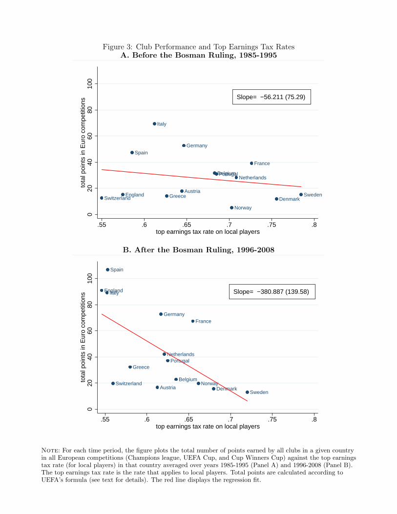
Figure 3: Club Performance and Top Earnings Tax RatesA. Before the Bosman Ruling, 1985-1995

Austria

Belgium

DenmarkEngland

France

Germany

Greece

Italy

Netherlands

Norway

Portugal

Spain

SwedenSwitzerland

Slope= −56.211 (75.29)0

2040

6080

100

tota

l poi

nts

in E

uro

com

petit

ions

.55 .6 .65 .7 .75 .8top earnings tax rate on local players

B. After the Bosman Ruling, 1996-2008

Austria

Belgium

Denmark

England

FranceGermany

Greece

Italy

Netherlands

Norway

Portugal

Spain

Sweden

Switzerland

Slope= −380.887 (139.58)

020

4060

8010

0to

tal p

oint

s in

Eur

o co

mpe

titio

ns

.55 .6 .65 .7 .75 .8top earnings tax rate on local players

Note: For each time period, the figure plots the total number of points earned by all clubs in a given countryin all European competitions (Champions league, UEFA Cup, and Cup Winners Cup) against the top earningstax rate (for local players) in that country averaged over years 1985-1995 (Panel A) and 1996-2008 (Panel B).The top earnings tax rate is the rate that applies to local players. Total points are calculated according toUEFA’s formula (see text for details). The red line displays the regression fit.

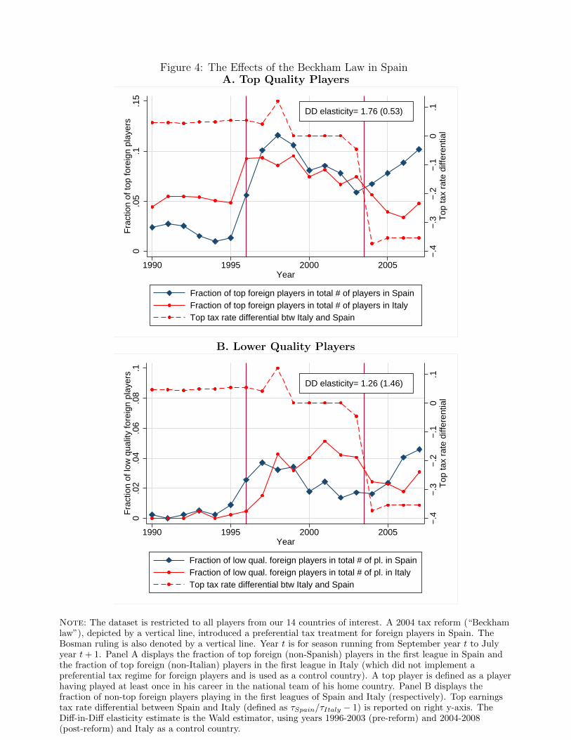
Figure 4: The Effects of the Beckham Law in SpainA. Top Quality Players

DD elasticity= 1.76 (0.53)

−.4

−.3

−.2

−.1

0.1

Top

tax

rate

diff

eren

tial

0.0

5.1

.15

Fra

ctio

n of

top

fore

ign

play

ers

1990 1995 2000 2005Year

Fraction of top foreign players in total # of players in SpainFraction of top foreign players in total # of players in ItalyTop tax rate differential btw Italy and Spain

B. Lower Quality Players

DD elasticity= 1.26 (1.46)

−.4

−.3

−.2

−.1

0.1

Top

tax

rate

diff

eren

tial

0.0

2.0

4.0

6.0

8.1

Fra

ctio

n of

low

qua

lity

fore

ign

play

ers

1990 1995 2000 2005Year

Fraction of low qual. foreign players in total # of pl. in SpainFraction of low qual. foreign players in total # of pl. in ItalyTop tax rate differential btw Italy and Spain

Note: The dataset is restricted to all players from our 14 countries of interest. A 2004 tax reform (“Beckhamlaw”), depicted by a vertical line, introduced a preferential tax treatment for foreign players in Spain. TheBosman ruling is also denoted by a vertical line. Year t is for season running from September year t to Julyyear t+ 1. Panel A displays the fraction of top foreign (non-Spanish) players in the first league in Spain andthe fraction of top foreign (non-Italian) players in the first league in Italy (which did not implement apreferential tax regime for foreign players and is used as a control country). A top player is defined as a playerhaving played at least once in his career in the national team of his home country. Panel B displays thefraction of non-top foreign players playing in the first leagues of Spain and Italy (respectively). Top earningstax rate differential between Spain and Italy (defined as τSpain/τItaly − 1) is reported on right y-axis. TheDiff-in-Diff elasticity estimate is the Wald estimator, using years 1996-2003 (pre-reform) and 2004-2008(post-reform) and Italy as a control country.

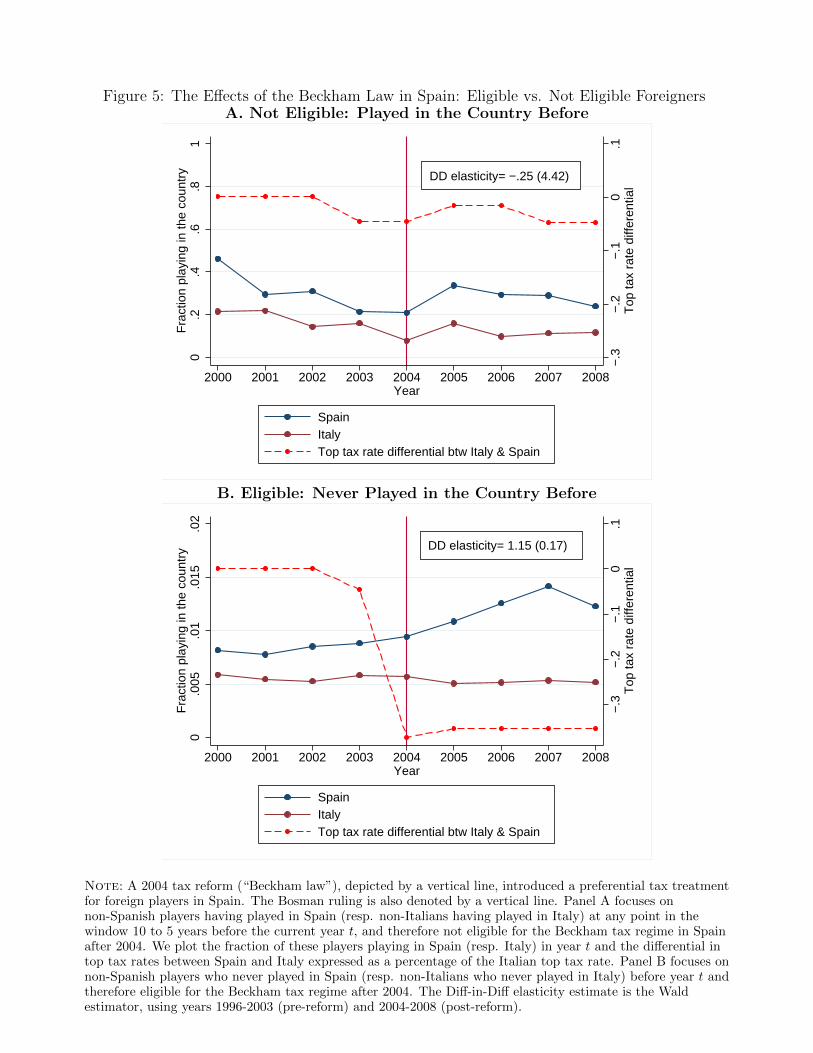
Figure 5: The Effects of the Beckham Law in Spain: Eligible vs. Not Eligible ForeignersA. Not Eligible: Played in the Country Before

DD elasticity= −.25 (4.42)

.10

−.1

−.2

−.3

Top

tax

rate

diff

eren

tial

0.2

.4.6

.81

Fra

ctio

n pl

ayin

g in

the

coun

try

2000 2001 2002 2003 2004 2005 2006 2007 2008Year

SpainItalyTop tax rate differential btw Italy & Spain

B. Eligible: Never Played in the Country Before

DD elasticity= 1.15 (0.17)

.10

−.1

−.2

−.3

Top

tax

rate

diff

eren

tial

0.0

05.0

1.0

15.0

2F

ract

ion

play

ing

in th

e co

untr

y

2000 2001 2002 2003 2004 2005 2006 2007 2008Year

SpainItalyTop tax rate differential btw Italy & Spain

Note: A 2004 tax reform (“Beckham law”), depicted by a vertical line, introduced a preferential tax treatmentfor foreign players in Spain. The Bosman ruling is also denoted by a vertical line. Panel A focuses onnon-Spanish players having played in Spain (resp. non-Italians having played in Italy) at any point in thewindow 10 to 5 years before the current year t, and therefore not eligible for the Beckham tax regime in Spainafter 2004. We plot the fraction of these players playing in Spain (resp. Italy) in year t and the differential intop tax rates between Spain and Italy expressed as a percentage of the Italian top tax rate. Panel B focuses onnon-Spanish players who never played in Spain (resp. non-Italians who never played in Italy) before year t andtherefore eligible for the Beckham tax regime after 2004. The Diff-in-Diff elasticity estimate is the Waldestimator, using years 1996-2003 (pre-reform) and 2004-2008 (post-reform).

Figure 6: Displacement Effects of the Beckham Law in Spain

050

100

150

200

250

Num

ber

of fo

reig

n pl

ayer

s

200

250

300

350

400

450

Num

ber

of d

omes

tic p

laye

rs

1985 1990 1995 2000 2005Year

Number of domestic players in SpainNumber of foreign players in Spain

Note: The dataset is restricted to all players from our 14 countries of interest. A 2004 tax reform (“Beckhamlaw”), depicted by a vertical line, introduced a preferential tax treatment for foreign players in Spain. TheBosman ruling is also denoted by a vertical line. Year t is for season running from September year t to Julyyear t+ 1. The graph displays the total number of local players who play in the first league of Spain and alsothe total number of foreign players (from the 14 European countries of interest) playing in the first league inSpain. Consistent with the existence of labor demand rigidity creating displacement effects, the total numberof Spanish players decreases after the Bosman ruling, and then after the introduction of the Beckham Law in2004, while the total number of foreign player increases. The Bosman Ruling and the Beckham Law haveattracted foreign players who have partially crowded-out local players.In 1995 and 1996, the Spanish League had 22 teams instead of the traditional 20 teams. To control for thisvariation in the size of the League, we removed from the sample the 2 lowest ranked teams in Spain in 1995and 1996, that would not have been part of the League had the number of teams remained the same.

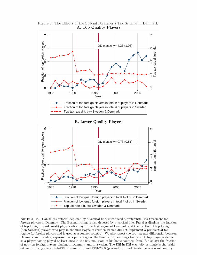
Figure 7: The Effects of the Special Foreigner’s Tax Scheme in DenmarkA. Top Quality Players

DD elasticity= 4.23 (1.03)

.20

−.2

−.4

−.6

Top

tax

rate

diff

eren

tial

0.0

25.0

5.0

75.1

Fra

ctio

n of

top

fore

ign

play

ers

1985 1990 1995 2000 2005Year

Fraction of top foreign players in total # of players in DenmarkFraction of top foreign players in total # of players in SwedenTop tax rate diff. btw Sweden & Denmark

B. Lower Quality Players

DD elasticity= 0.73 (0.51)

.20

−.2

−.4

−.6

Top

tax

rate

diff

eren

tial

0.0

5.1

.15

Fra

ctio

n of

low

qua

l. fo

reig

n pl

ayer

s

1985 1990 1995 2000 2005Year

Fraction of low qual. foreign players in total # of pl. in DenmarkFraction of low qual. foreign players in total # of pl. in SwedenTop tax rate diff. btw Sweden & Denmark

Note: A 1991 Danish tax reform, depicted by a vertical line, introduced a preferential tax treatment forforeign players in Denmark. The Bosman ruling is also denoted by a vertical line. Panel A displays the fractionof top foreign (non-Danish) players who play in the first league of Denmark and the fraction of top foreign(non-Swedish) players who play in the first league of Sweden (which did not implement a preferential taxregime for foreign players and is used as a control country). We also report the top tax rate differential betweenDenmark and Sweden, expressed as a percentage of the Swedish top earnings tax rate. A top player is definedas a player having played at least once in the national team of his home country. Panel B displays the fractionof non-top foreign players playing in Denmark and in Sweden. The Diff-in-Diff elasticity estimate is the Waldestimator, using years 1985-1990 (pre-reform) and 1991-2008 (post-reform) and Sweden as a control country.

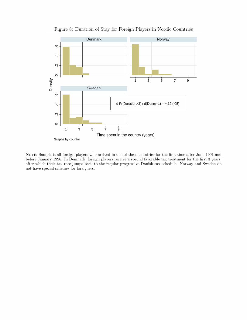
Figure 8: Duration of Stay for Foreign Players in Nordic Countries

0.2

.4.6

0.2

.4.6

1 3 5 7 9

1 3 5 7 9

Denmark Norway

Sweden

d Pr(Duration>3) / d(Denm=1) = −.12 (.05)

Den

sity

Time spent in the country (years)Graphs by country

Note: Sample is all foreign players who arrived in one of these countries for the first time after June 1991 andbefore January 1996. In Denmark, foreign players receive a special favorable tax treatment for the first 3 years,after which their tax rate jumps back to the regular progressive Danish tax schedule. Norway and Sweden donot have special schemes for foreigners.

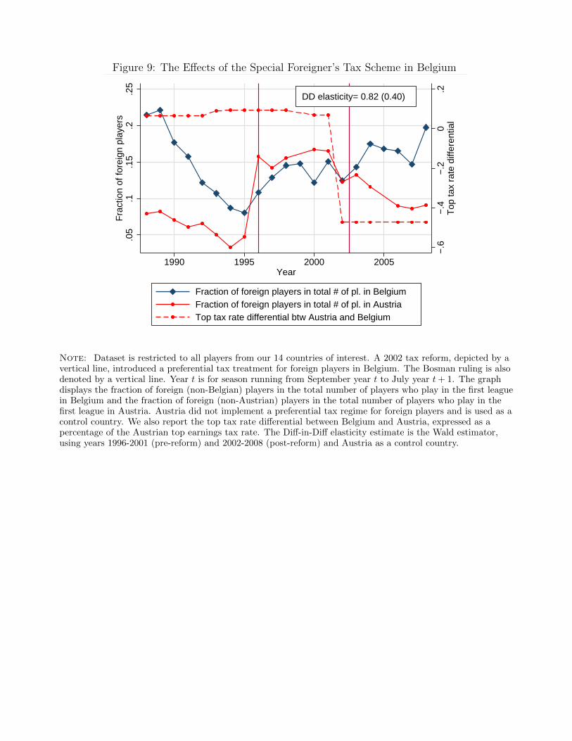
Figure 9: The Effects of the Special Foreigner’s Tax Scheme in Belgium

DD elasticity= 0.82 (0.40)

−.6

−.4

−.2

0.2

Top

tax

rate

diff

eren

tial

.05

.1.1

5.2

.25

Fra

ctio

n of

fore

ign

play

ers

1990 1995 2000 2005Year

Fraction of foreign players in total # of pl. in BelgiumFraction of foreign players in total # of pl. in AustriaTop tax rate differential btw Austria and Belgium

Note: Dataset is restricted to all players from our 14 countries of interest. A 2002 tax reform, depicted by avertical line, introduced a preferential tax treatment for foreign players in Belgium. The Bosman ruling is alsodenoted by a vertical line. Year t is for season running from September year t to July year t+ 1. The graphdisplays the fraction of foreign (non-Belgian) players in the total number of players who play in the first leaguein Belgium and the fraction of foreign (non-Austrian) players in the total number of players who play in thefirst league in Austria. Austria did not implement a preferential tax regime for foreign players and is used as acontrol country. We also report the top tax rate differential between Belgium and Austria, expressed as apercentage of the Austrian top earnings tax rate. The Diff-in-Diff elasticity estimate is the Wald estimator,using years 1996-2001 (pre-reform) and 2002-2008 (post-reform) and Austria as a control country.

Figure 10: Decreasing Labor Demand for Football PlayersA. Average Number of Players per Team and Top Earnings Tax Rates

Austria

BelgiumDenmark

England

France

Germany

Greece

Italy

Netherlands

Norway

Portugal

Spain

SwedenSwitzerland

2530

3540

Ave

rage

num

ber

of p

laye

rs b

y te

am

.55 .6 .65 .7 .75top earnings tax rate

B. Average Number of Teams per League and Top Earnings Tax Rates

Austria

Belgium

Denmark

England

France

Germany

Greece

Italy

Netherlands

Norway

Portugal

Spain

Sweden

Switzerland

1012

1416

1820

Ave

rage

num

ber

of te

ams

by c

ount

ry

.55 .6 .65 .7 .75top earnings tax rate

Note: Panel A: Each dot shows the average number of players per team and the weighted average of topearnings tax rate for local and foreign players for years 1995 to 2009.Panel B: Each dot shows the average number of teams per League and the weighted average of top earningstax rate for local and foreign players for years 1995 to 2009. The red line displays the regression fit.

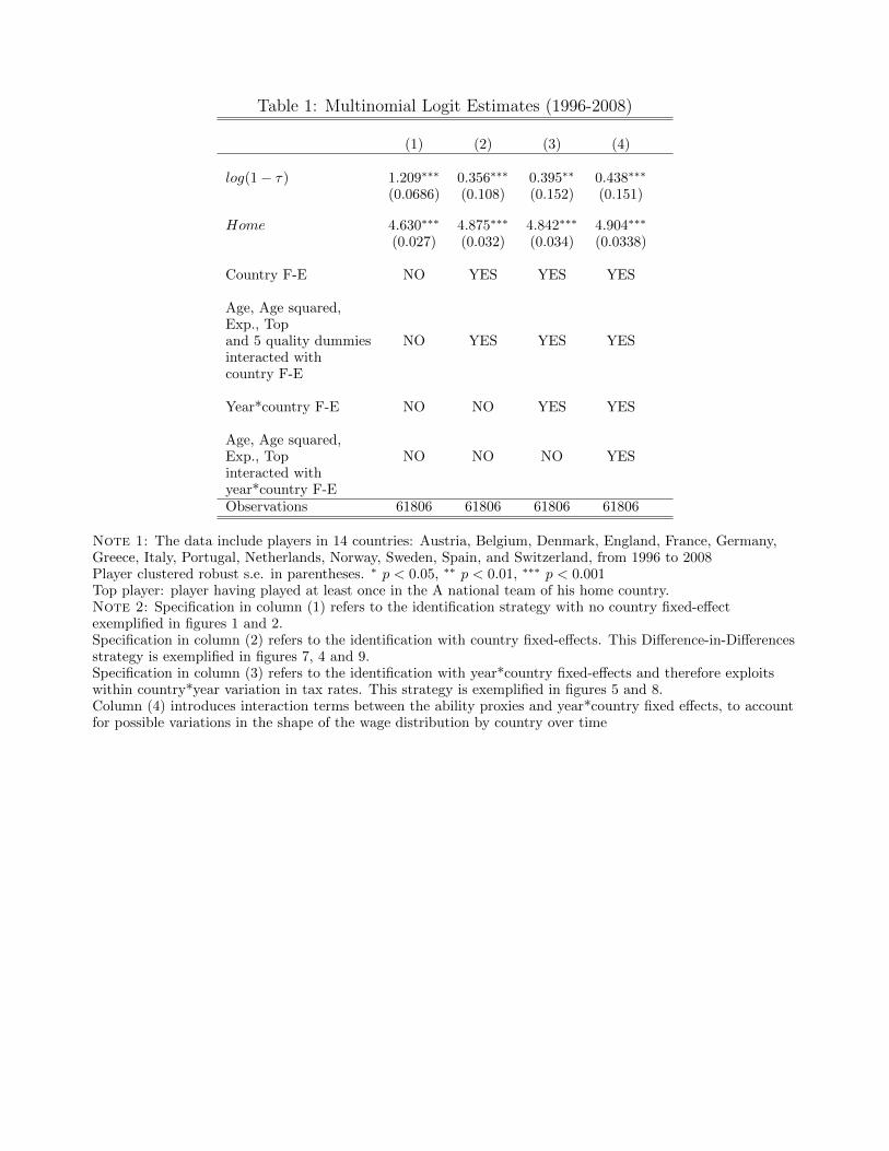
Table 1: Multinomial Logit Estimates (1996-2008)

(1) (2) (3) (4)

log(1− τ) 1.209∗∗∗ 0.356∗∗∗ 0.395∗∗ 0.438∗∗∗

(0.0686) (0.108) (0.152) (0.151)

Home 4.630∗∗∗ 4.875∗∗∗ 4.842∗∗∗ 4.904∗∗∗

(0.027) (0.032) (0.034) (0.0338)

Country F-E NO YES YES YES

Age, Age squared,Exp., Topand 5 quality dummies NO YES YES YESinteracted withcountry F-E

Year*country F-E NO NO YES YES

Age, Age squared,Exp., Top NO NO NO YESinteracted withyear*country F-EObservations 61806 61806 61806 61806

Note 1: The data include players in 14 countries: Austria, Belgium, Denmark, England, France, Germany,Greece, Italy, Portugal, Netherlands, Norway, Sweden, Spain, and Switzerland, from 1996 to 2008Player clustered robust s.e. in parentheses. ∗ p < 0.05, ∗∗ p < 0.01, ∗∗∗ p < 0.001Top player: player having played at least once in the A national team of his home country.Note 2: Specification in column (1) refers to the identification strategy with no country fixed-effectexemplified in figures 1 and 2.Specification in column (2) refers to the identification with country fixed-effects. This Difference-in-Differencesstrategy is exemplified in figures 7, 4 and 9.Specification in column (3) refers to the identification with year*country fixed-effects and therefore exploitswithin country*year variation in tax rates. This strategy is exemplified in figures 5 and 8.Column (4) introduces interaction terms between the ability proxies and year*country fixed effects, to accountfor possible variations in the shape of the wage distribution by country over time

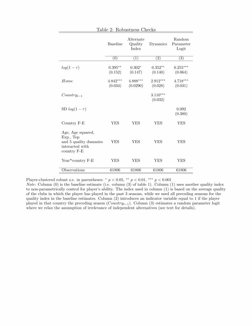
Table 2: Robustness Checks

Alternate RandomBaseline Quality Dynamics Parameter

Index Logit

(0) (1) (2) (3)

log(1− τ) 0.395∗∗ 0.302∗ 0.352∗∗ 0.255∗∗∗

(0.152) (0.147) (0.140) (0.064)

Home 4.842∗∗∗ 4.888∗∗∗ 2.912∗∗∗ 4.718∗∗∗

(0.034) (0.0290) (0.028) (0.031)

Countryt−1 3.110∗∗∗

(0.032)

SD log(1− τ) 0.092(0.380)

Country F-E YES YES YES YES

Age, Age squared,Exp., Topand 5 quality dummies YES YES YES YESinteracted withcountry F-E

Year*country F-E YES YES YES YES

Observations 61806 61806 61806 61806

Player-clustered robust s.e. in parentheses: ∗ p < 0.05, ∗∗ p < 0.01, ∗∗∗ p < 0.001Note: Column (0) is the baseline estimate (i.e. column (3) of table 1). Column (1) uses another quality indexto non-parametrically control for player’s ability. The index used in column (1) is based on the average qualityof the clubs in which the player has played in the past 3 seasons, while we used all preceding seasons for thequality index in the baseline estimates. Column (2) introduces an indicator variable equal to 1 if the playerplayed in that country the preceding season (Countryt−1). Column (3) estimates a random parameter logitwhere we relax the assumption of irrelevance of independent alternatives (see text for details).

Table 3: Multinomial Logit Estimates Including Sorting Effects and Displacement Effects

Sorting Sorting Sorting Sorting+ Displacement + Displacement

Long Short Long Short Long Short Long Shortterm term term term term term term term(1) (2) (3) (4) (5) (6) (7) (8)

log(1− τ) ∗ low -0.342∗∗ -0.251∗ -0.394∗∗ -0.285∗

(0.124) (0.123) (0.120) (0.119)

log(1− τ) ∗ top 1.539∗∗∗ 1.293∗∗∗ 1.409∗∗∗ 1.209∗∗∗

(0.182) (0.179) (0.179) (0.177)

log(1− τ) ∗Qual0−25 -0.233 -0.791∗∗∗ -0.329∗∗ -0.811∗∗∗

(0.126) (0.144) (0.126) (0.138)

log(1− τ) ∗Qual25−50 -0.609∗∗∗ 0.215 -0.722∗∗∗ 0.116(0.163) (0.171) (0.163) (0.172)

log(1− τ) ∗Qual50−75 0.453∗∗ 0.785∗∗∗ 0.332∗ 0.699∗∗∗

(0.171) (0.184) (0.169) (0.179)

log(1− τ) ∗Qual75−95 1.911∗∗∗ 1.356∗∗∗ 1.852∗∗∗ 1.379∗∗∗

(0.160) (0.256) (0.158) (0.247)

log(1− τ) ∗Qual95−100 2.275∗∗∗ 0.307 2.229∗∗∗ 0.487(0.335) (0.754) (0.329) (0.713)

log(1− τf ) ∗ domestic -0.875∗∗∗ -0.819∗∗∗ -0.956∗∗∗ -0.869∗∗∗

(0.128) (0.127) (0.127) (0.128)

log(1− τd) ∗ foreign -0.0447 -0.0291 -0.144 -0.136(0.177) (0.176) (0.174) (0.180)

Home 4.868∗∗∗ 4.792∗∗∗ 4.172∗∗∗ 4.127∗∗∗ 4.872∗∗∗ 4.798∗∗∗ 4.206∗∗∗ 4.196∗∗∗

(0.031) (0.032) (0.173) (0.176) (0.032) (0.032) (0.172) (0.177)

Age, Age squared,Exp., Topinteracted with YES YES YES YES YES YES YES YEScountry F-E

5 quality dummiesinteracted with NO YES NO YES NO YES NO YEScountry F-E

Observations 61806 61806 61806 61806 61806 61806 61806 61806

Player-clustered robust s.e. in parentheses: ∗ p < 0.05, ∗∗ p < 0.01, ∗∗∗ p < 0.001top is an indicator variable for having played at least once in the home country national team (proxy for beinga top quality player). Conversely low is defined as non-top. Qual0−25: Players with quality index below the25th percentile of the quality index that given year, etc. The quality index is defined in the text in detail. Theinteraction between quality and log(1− τ) captures the sorting effects.For the country c where the individual is currently playing, τf is the tax rate that applies in country c toforeign players and τd is the tax rate on local players in country c. domestic (resp. foreign) is an indicatorvariable for being a domestic (resp. foreign) player. Those variables capture the displacement effects that arisein the rigid labor demand model.

Table 4: Revenue Maximizing Tax Rates on Football Players

Top Earnings Revenue MaximizingTax Rates Tax Rates

(2008)Flexible RigidLabor Labor

Demand Demand

Domestic Foreign τ∗ τ∗ τ∗f(1) (2) (3) (4) (5)

Austria 0.612 0.612 0.764 0.843 0.799Belgium 0.616 0.322 0.769 0.888 0.516Denmark 0.698 0.448 0.768 0.791 0.667

UK 0.552 0.552 0.817 0.949 0.430France 0.611 0.524 0.769 0.860 0.999

Germany 0.593 0.593 0.773 0.934 0.539Greece 0.496 0.496 0.761 0.995 0.486Italy 0.534 0.534 0.776 0.951 0.568

Netherlands 0.597 0.466 0.769 0.888 0.545Norway 0.608 0.582 0.768 0.856 0.722Portugal 0.654 0.654 0.761 0.838 0.989

Spain 0.509 0.345 0.801 0.941 0.560Sweden 0.738 0.738 0.771 0.989 0.999

Switzerland 0.561 0.561 0.767 0.896 0.535

Notes: Columns (1) and (2) report the top earnings tax rate in each country in 2008 that apply to domesticand foreign players respectively. Column (3) computes the revenue maximizing tax rate on all football players(where both domestic and foreign players face the same tax rate) in the case of perfectly elastic labor demand.In this case, as shown in Proposition 1, the standard inverse supply elasticity rule applies. We compute thewage weighted supply elasticity according to our baseline estimates in column (3) of table 1. Wage weights foreach quality group are computed using data on all wages in the Italian League for the 2001 season. We wouldlike to thank Pr. Lucifora for sharing these data with us. The aggregate elasticity is the weighted average ofthe elasticity for the different quality groups.Column (4) computes the revenue maximizing tax rate on all football players (where both domestic and foreignplayers face the same tax rate) taking into account displacement and sorting effects, following the formulapresented in Proposition 2. The aggregate elasticity is the wage weighted average of the elasticity of foreignersand domestic players taking into account sorting effects and displacement effect estimates of column (7) oftable 3.Column (5) computes the revenue maximizing tax rate on foreign players specifically (and assuming that thetax rate on domestic players stays the same as it is in 2008 in each country) taking into account displacementand sorting effects, following the formula presented in Proposition 2. The elasticities of foreign and domesticplayers w.r.t foreigner tax rates are also wage weighted, and computed according to estimates of column (7) oftable 3.

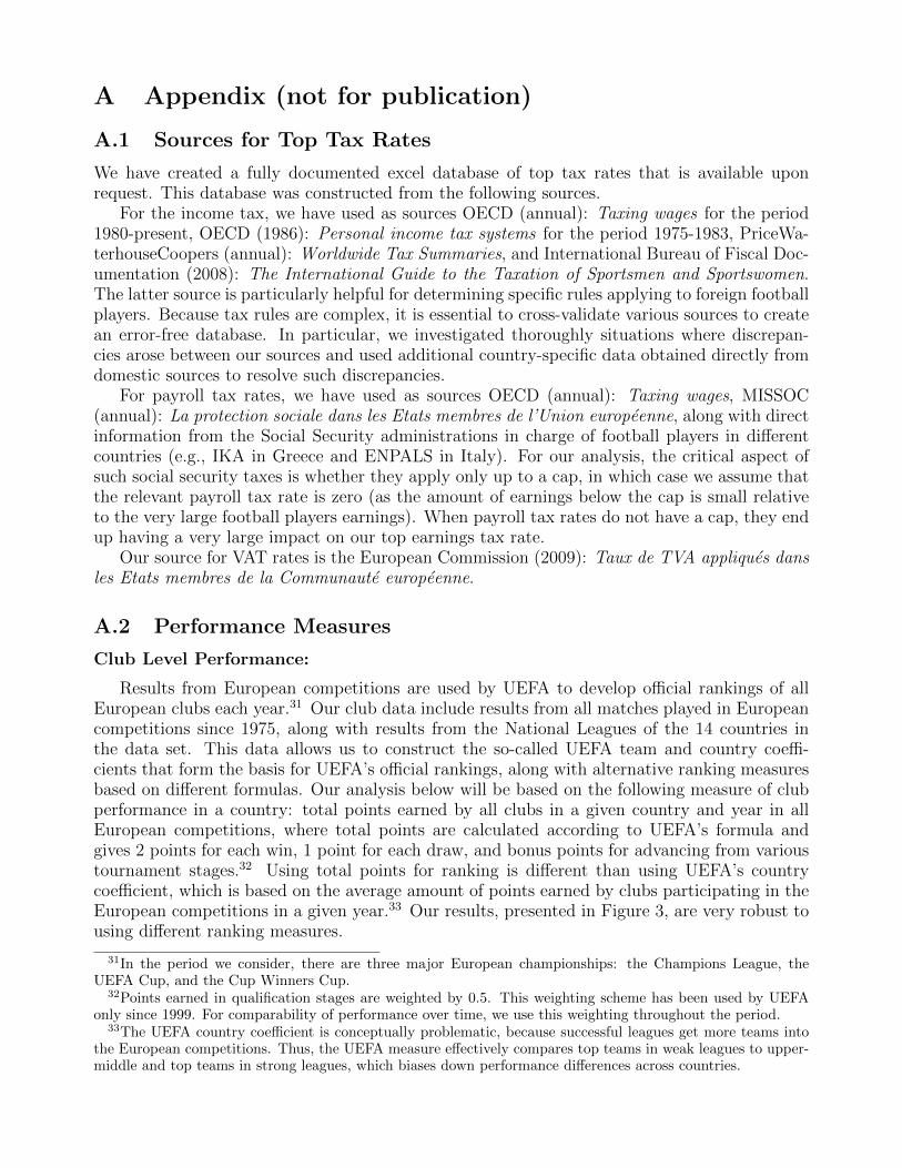
A Appendix (not for publication)

A.1 Sources for Top Tax Rates

We have created a fully documented excel database of top tax rates that is available uponrequest. This database was constructed from the following sources.

For the income tax, we have used as sources OECD (annual): Taxing wages for the period1980-present, OECD (1986): Personal income tax systems for the period 1975-1983, PriceWa-terhouseCoopers (annual): Worldwide Tax Summaries, and International Bureau of Fiscal Doc-umentation (2008): The International Guide to the Taxation of Sportsmen and Sportswomen.The latter source is particularly helpful for determining specific rules applying to foreign footballplayers. Because tax rules are complex, it is essential to cross-validate various sources to createan error-free database. In particular, we investigated thoroughly situations where discrepan-cies arose between our sources and used additional country-specific data obtained directly fromdomestic sources to resolve such discrepancies.

For payroll tax rates, we have used as sources OECD (annual): Taxing wages, MISSOC(annual): La protection sociale dans les Etats membres de l’Union europeenne, along with directinformation from the Social Security administrations in charge of football players in differentcountries (e.g., IKA in Greece and ENPALS in Italy). For our analysis, the critical aspect ofsuch social security taxes is whether they apply only up to a cap, in which case we assume thatthe relevant payroll tax rate is zero (as the amount of earnings below the cap is small relativeto the very large football players earnings). When payroll tax rates do not have a cap, they endup having a very large impact on our top earnings tax rate.

Our source for VAT rates is the European Commission (2009): Taux de TVA appliques dansles Etats membres de la Communaute europeenne.

A.2 Performance Measures

Club Level Performance:

Results from European competitions are used by UEFA to develop official rankings of allEuropean clubs each year.31 Our club data include results from all matches played in Europeancompetitions since 1975, along with results from the National Leagues of the 14 countries inthe data set. This data allows us to construct the so-called UEFA team and country coeffi-cients that form the basis for UEFA’s official rankings, along with alternative ranking measuresbased on different formulas. Our analysis below will be based on the following measure of clubperformance in a country: total points earned by all clubs in a given country and year in allEuropean competitions, where total points are calculated according to UEFA’s formula andgives 2 points for each win, 1 point for each draw, and bonus points for advancing from varioustournament stages.32 Using total points for ranking is different than using UEFA’s countrycoefficient, which is based on the average amount of points earned by clubs participating in theEuropean competitions in a given year.33 Our results, presented in Figure 3, are very robust tousing different ranking measures.

31In the period we consider, there are three major European championships: the Champions League, theUEFA Cup, and the Cup Winners Cup.

32Points earned in qualification stages are weighted by 0.5. This weighting scheme has been used by UEFAonly since 1999. For comparability of performance over time, we use this weighting throughout the period.

33The UEFA country coefficient is conceptually problematic, because successful leagues get more teams intothe European competitions. Thus, the UEFA measure effectively compares top teams in weak leagues to upper-middle and top teams in strong leagues, which biases down performance differences across countries.

Individual Quality Index:

The empirical estimation of Section 5 uses an individual player quality index. The compu-tation of this index requires the following three steps.

(i) For each club k in country n in year t, we compute a club quality measure (Qk,n,t) basedon the ranking of the club in the national league of country n (league rankk,n,t) combined witha country coefficient measuring the international standing of the league (country coefn,t). Asdescribed in Section 2, the country coefficient is equal to the total number of points earned byall clubs in the country in a given year in all UEFA competitions. Club quality is then measuredas

Qk,n,t =

[maxk(league rankk,n,t)− league rankk,n,t + 1

maxk(league rankk,n,t)

]2

× country coefn,t (13)

The term in brackets term runs from 1 for the best club to 1/maxk(league rankk,n,t) for theworst club in the league. We square this term to account for skewness in the distribution ofclub quality within countries.34

(ii) We then assign to each player in year t a value V it given by the average quality of all

the clubs he has played for from the beginning of his professional career until year t − 1. Forrobustness, we also construct a measure of V i

t equal to the average quality of the clubs he hasplayed for during the three preceding seasons t− 3, t− 2, and t− 1.35

(iii) We finally rank all players in year t according to V it , and assign to each player his

quantile position in the distribution of V it .36

A.3 Proofs of Theoretical Results

Proof of Proposition 1:

(a) Total revenue is given by

Rn = τn

∫ ∞0

apnada,

where pna = pna (a (1− τn)) ≡ pnda (a (1− τn)) + pnfa (a (1− τn)). The Laffer rate τ ∗n satisfies

dRn

dτn=

∫ ∞0

apnada−τ ∗n

1− τ ∗n

∫ ∞0

apnaεnada = 0,

where εna ≡ ∂pna

∂(1−τn)1−τnpna

. Hence,

τ ∗n1− τ ∗n

=1

εn,

where εn ≡∫∞0 apnaεnada∫∞

0 apnada. This corresponds to eq. (5).

34We have checked that our results are robust to a club-quality index that does not square the league rankingterm.

35We include club points only until year t − 1 to avoid correlation between the quality index V it of player i

in year t and the migration choice of this player in year t. Notice also that averaging club quality over a careerof course does not eradicate a correlation between our player quality index and age, because players tend toadvance to better clubs over the career path. This is the reason why we always control directly for age andexperience in our regressions.

36As mentioned earlier, we have data on player salaries for all players in the Italian league in 2001. Hence, forthis country and year, we can check the correlation between our ability index and actual salaries. Even withoutcontrolling for the other quality measures (age, experience, and national team selection), our quality index isstrongly positively correlated with player salaries, suggesting that we measure player ability quite well.

(b) Total revenue is given by

Rn = τnd

∫ ∞0

apndada+ τnf

∫ ∞0

apnfada,

where pnda = pnda (a (1− τnd)) and pnfa = pnfa (a (1− τnf )). For the Laffer rate τ ∗nd, we get

dRn

dτnd=

∫ ∞0

apndada−τ ∗nd

1− τ ∗nd

∫ ∞0

apndaεndada = 0,

where εnda ≡ ∂pnda

∂(1−τnd)1−τnd

pnda. Hence,

τ ∗nd1− τ ∗nd

=1

εnd,

where εnd ≡∫∞0 apndaεndada∫∞

0 apndada. This corresponds to the first part of eq. (6). The proof for τ ∗nf

follows symmetrically. �

Proof of Proposition 2:

(a) Given the presence of positive club surpluses, we have to make an assumption about thetaxation of these surpluses. We assume that club surplus is taxed at the same rate as playerearnings, so that the division of value added into club surplus sn and player earnings a − snhas no mechanical impact on government revenue (note though that changes in sn does havea behavioral revenue effect from changed migration). Under this simplifying assumption, totaltax revenue collected from the football sector is given by

Rn = τn

∫ ∞sn

apnada,

where pna = pna (1− τn) = pnda (1− τn) + pnfa (1− τn). We work with general equilibriumrelationships, which is why sn does not appear as an argument in pna (.). The Laffer rate τ ∗nsatisfies

dRn

dτn=

∫ ∞sn

apnada−τ ∗n

1− τ ∗n

∫ ∞sn

apnaεnada = 0,

where εna ≡ ∂pna

∂(1−τn)1−τnpna

. Hence,

τ ∗n1− τ ∗n

=1

εn,

where εn ≡∫∞snapnaεnada∫∞

snapnada

. This corresponds to eq. (7).

(b) As above, we eliminate mechanical revenue effects of changes in sn by assuming that thetax rate on club surplus corresponds to the (average) tax rate on earnings. For the case ofa selective tax system (τnd, τnf ) and denoting the tax rate on club surplus by tn, we assumetn = τnd · pnd + τnf · pnf . Under this simplifying assumption, total tax revenue collected fromthe football sector can be written as

Rn = τnd

∫ ∞sn

apndada+ τnf

∫ ∞sn

apnfada,

where pnda = pnda (1− τnd, 1− τnf ) and pnfa = pnfa (1− τnd, 1− τnf ). Consider the Laffer rateon foreigners τ ∗nf given the tax rate on locals τnd. We can write the first-order condition as∫ ∞

sn

apnfada−τ ∗nf

1− τ ∗nf

∫ ∞sn

apnfaεnfada−τnd

1− τ ∗nf

∫ ∞sn

apndaσndada = 0,

where εnfa ≡ ∂pnfa

∂(1−τnf )

1−τnf

pnfa≥ 0 and σnda ≡ ∂pnda

∂(1−τnf )

1−τnf

pnda≤ 0. Defining ability-weighted average

elasticities

εnf ≡∫∞snapnfaεnfada∫∞snapnfada

, σnd ≡∫∞snapndaσndada∫∞snapndada

,

as well as total value-added generated by domestic and foreign players

znd ≡∫ ∞sn

apndada, znf ≡∫ ∞sn

apnfada,

we obtain the following expression

1−τ ∗nf

1− τ ∗nfεnf −

τnd1− τ ∗nf

zndznf

σnd = 0,

which can be rewritten to

τ ∗nf =1

1 + εnf

{1− τndσnd

(zndznf

)},

as in eq. (8). The proof for τ ∗nd follows symmetrically. �

Appendix ReferencesEuropean Commission (2009). Taux de TVA appliques dans les Etats membres de la Com-munaute europeenne.International Bureau of Fiscal Documentation (2008). The International Guide to theTaxation of Sportsmen and Sportswomen.MISSOC (annual). La protection sociale dans les etats membres de l’union europeenne.OECD (annual). Taxing wages, OECD, Paris.OECD (1986). Personal income tax systems, OECD, Paris.PriceWaterhouseCoopers (annual). Worldwide Tax Summaries.

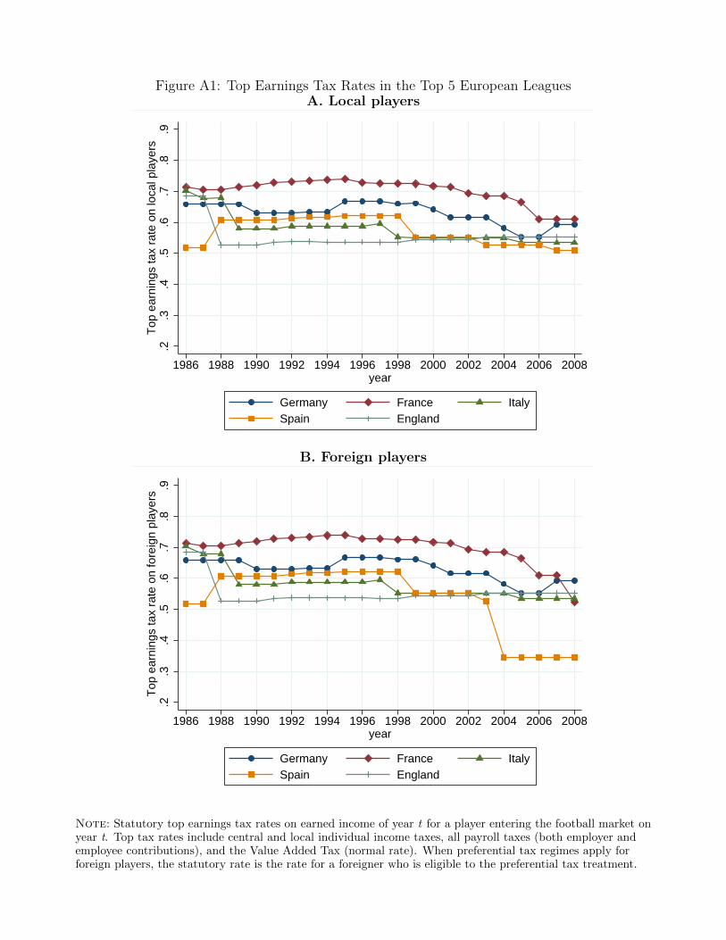
Figure A1: Top Earnings Tax Rates in the Top 5 European LeaguesA. Local players

.2.3

.4.5

.6.7

.8.9

Top

ear

ning

s ta

x ra

te o

n lo

cal p

laye

rs

1986 1988 1990 1992 1994 1996 1998 2000 2002 2004 2006 2008year

Germany France ItalySpain England

B. Foreign players

.2.3

.4.5

.6.7

.8.9

Top

ear

ning

s ta

x ra

te o

n fo

reig

n pl

ayer

s

1986 1988 1990 1992 1994 1996 1998 2000 2002 2004 2006 2008year

Germany France ItalySpain England

Note: Statutory top earnings tax rates on earned income of year t for a player entering the football market onyear t. Top tax rates include central and local individual income taxes, all payroll taxes (both employer andemployee contributions), and the Value Added Tax (normal rate). When preferential tax regimes apply forforeign players, the statutory rate is the rate for a foreigner who is eligible to the preferential tax treatment.

Figure A2: Top Earnings Tax Rates in Nordic CountriesA. Local players

.2.3

.4.5

.6.7

.8.9

Top

ear

ning

s ta

x ra

te o

n lo

cal p

laye

rs

1986 1988 1990 1992 1994 1996 1998 2000 2002 2004 2006 2008year

Denmark Norway Sweden

B. Foreign players

.2.3

.4.5

.6.7

.8.9

Top

ear

ning

s ta

x ra

te o

n fo

reig

n pl

ayer

s

1986 1988 1990 1992 1994 1996 1998 2000 2002 2004 2006 2008year

Denmark Norway Sweden

Note: Statutory top earnings tax rates on earned income of year t for a player entering the football market onyear t. Top tax rates include central and local individual income taxes, all payroll taxes (both employer andemployee contributions), and the Value Added Tax (normal rate). When preferential tax regimes apply forforeign players, the statutory rate is the rate for a foreigner who is eligible to the preferential tax treatment.

Figure A3: Top Earnings Tax Rates in the Smaller European LeaguesA. Local players

.2.3

.4.5

.6.7

.8.9

Top

ear

ning

s ta

x ra

te o

n lo

cal p

laye

rs

1986 1988 1990 1992 1994 1996 1998 2000 2002 2004 2006 2008year

Austria Belgium GreeceNetherlands Portugal Switzerland

B. Foreign players

.2.3

.4.5

.6.7

.8.9

Top

ear

ning

s ta

x ra

te o

n fo

reig

n pl

ayer

s

1986 1988 1990 1992 1994 1996 1998 2000 2002 2004 2006 2008year

Austria Belgium GreeceNetherlands Portugal Switzerland

Note: Statutory top earnings tax rates on earned income of year t for a player entering the football market onyear t. Top tax rates include central and local individual income taxes, all payroll taxes (both employer andemployee contributions), and the Value Added Tax (normal rate). When preferential tax regimes apply forforeign players, the statutory rate is the rate for a foreigner who is eligible to the preferential tax treatment.