Taxes on Tax-Exempt Bonds∗

Andrew Ang†

Columbia University and NBER

Vineer Bhansali‡

PIMCO

Yuhang Xing§

Rice University

This Version: 10 September 2008

JEL Classification: G12, G28, H20, H24Keywords: municipal bonds, income and capital gains tax,

de minimis boundary, public finance, implicit tax rate

∗We thank Mark McCray, Aron Gereben, Rick Green, Cam Harvey, Gur Huberman, Dan Li, BobMcDonald, Jeffrey Pontiff, and Andrew Schmidt for helpful discussions. We are especially gratefulto Jeff Strnad for providing detailed comments. The paper has benefited from truly excellent commentsfrom an anonymous referee and the editor. We thank seminar participants at the High Frequency Data andBond Markets Conference at the University of Cambridge, the Western Finance Association, BrighamYoung University, Columbia University, European Central Bank, Fordham University, Georgia StateUniversity, Ohio State University, Rutgers University, Shanghai JiaoTong University, UC Irvine, and UCSan Diego. We also thank Philippe Mueller for tabulating some of the data and Jihong Zang for checkingsome law sources.

†Columbia Business School, 3022 Broadway 413 Uris, New York, NY 10027. Ph: (212) 854-9154,Email: aa610@columbia.edu, WWW: http://www.columbia.edu/∼aa610.

‡PIMCO, 840 Newport Center Drive, Suite 100, Newport Beach, CA 92660. Ph: (949) 720-6333,Email: Vineer.Bhansali@pimco.com

§Jones School of Management, Rice University, Rm 342, MS 531, 6100 Main Street, Houston, TX77004. Ph: (713) 348-4167, Email: yxing@rice.edu.

Taxes on Tax-Exempt Bonds

Abstract

Implicit tax rates priced in the cross section of municipal bonds are approximately two to

three times as high as statutory income tax rates, with implicit tax rates close to 100% using

retail trades and above 70% for interdealer trades. These implied tax rates can be identified on

the cross section of municipal bonds because a portion of secondary market municipal bond

trades involve income taxes. After valuing the tax payments, market discount bonds, which

carry income tax liabilities, trade at yields around 25 basis points higher than comparable mu-

nicipal bonds not subject to any taxes. The high sensitivities of municipal bond prices to tax

rates can be traced to individual retail traders dominating dealers and other institutions.

1 Introduction

The issue of how taxes affect the prices of assets is an important issue in finance, accounting,

and economics. In theoretical models examining the effect of taxes on different assets and

different agents (for example, Auerbach and King, 1983; Dybvig and Ross, 1986; Dammon and

Green, 1987), taxes induce clientele effects in the asset holdings of agents and the existence of

different tax rates affects relative asset prices. In reality, estimating implicit tax rates on assets

is more difficult than theoretical models suggest because of the myriad ways the tax code can

be distorted, large investor heterogeneity, and the many different degrees of market frictions

faced by different investors. These real-world issues are especially true for investigating if the

tax rates faced by individual investors, as opposed to the tax rates faced by corporations, affect

asset prices because financial markets are often dominated by financial institutions and dealers.

For example, studies using equities find little evidence of implicit tax effects (see, among many

others, Boyd and Jagannathan, 1994; Fama and French, 1998; Erickson and Maydew, 1998). In

Treasury markets, Green and Ødegaard (1993) find that after the 1986 tax reform, the marginal

investor in Treasury bonds has a marginal tax rate of zero.

In contrast to government bonds and equities, the municipal bond market is well suited to

evaluate how individual tax rates affect asset prices. First, the municipal bond market is large;

the Flow of Funds data from the Federal Reserve show that at the end of the first quarter of 2007,

there were $2.5 trillion outstanding municipal securities compared to $4.8 trillion Treasuries.

Second, municipal bonds are attractive to high net worth individuals. Not surprisingly, individ-

ual holdings of municipal bonds dominate the holdings of other corporate entities. At the end of

the first quarter of 2007, individuals held 70% of all outstanding municipal bonds. Individuals

directly held 36% of all municipal securities outstanding and held 34% through mutual funds,

closed-end funds, and other taxable pass-through intermediaries.1

Third, individual investors are the marginal pricers in the municipal bond market at an ag-

gregate level, from the fact that the municipal yield curve trades lower than the Treasury yield

curve. Short-maturity municipal yields are equal to the Treasury yield times one minus the

income tax rate and the ratio between municipal and Treasury yields decreases with maturity.

These stylized facts are matched well by Green’s (1993) model, where after-tax yields on mu-

nicipal and Treasury bonds are equalized by individuals, in contrast to the Treasury market

1 The remainder was held mostly by banks and insurance companies. The proportion of municipal bonds held

directly and indirectly by individuals has been well above 70% over our post-1995 sample period, but was around

35% pre-1985. (See Hildreth and Zorn, 2005, for a history of developments in the municipal market.)

1

where tax-exempt institutions and dealers dominate pricing. Since at an asset class level indi-

vidual investors set the prices of municipal bonds relative to Treasury securities, we would also

expect individual tax rates to affect the cross-sectional pricing of municipal securities.

It would be impossible to study the effect of individual tax rates in the relative prices of

municipal bonds if all municipal securities had identical tax treatment with all cashflows exempt

from tax.2 Fortunately, this is not the case. A unique feature of the municipal bond market is

at any given time, an individual investor can purchase municipal bonds which are fully tax

exempt, where all the bond cashflows are not subject to tax, or municipal bonds subject to

income tax or capital gains tax. Municipal bonds bearing income tax liabilities are termed

market discount bonds. We exploit this cross-sectional heterogeneity to estimate the effects of

individual tax rates on municipal bond prices as well as to characterize how different investor

clienteles respond to different tax treatments. Furthermore, the same bond may change its

tax treatment over time, changing from say being subject to income tax to becoming fully tax

exempt. Thus, we can also identify the effect of taxes from the time series of these bonds as

they move across tax boundaries.

The existence of fully tax-exempt bonds together with municipal bonds subject to income

or capital gains tax arises from how the tax code defines market discount. When a municipal

bond is issued, the coupon payments and original issue discount (OID) are exempt from federal

income tax. However, the profits from trading municipal bonds in secondary markets are tax-

able. If market discount exists, which in most situations is defined as a large enough difference

between the market price and par value for a bond issued at par, the purchaser of the bond is

liable for income tax, otherwise taxes are levied at capital gains rates. These taxes depend on

the purchase price of the bond, the bond’s original issue yield or price, and original maturity.

While most municipal bond trades are not subject to tax, there is an important subset of munic-

ipal bond transactions involving bonds subject to income tax. In some years trades involving

market discount bonds represent over 30% of all transactions.

Since 1993, market discount is taxed at regular income tax rates. The Internal Revenue Code

(IRC) allows small amounts of market discount to be considered zero and be treated as capital

gains, which is termed the de minimis exemption. That is, below the de minimis boundary,

market discount is taxed as income. Above the de minimis boundary, bonds may be subject to

capital gains tax. If a par bond is trading above par all bond cashflows are not subject to tax.

2 A small number of municipal bonds do not have tax-exempt cashflows, such as private activity bonds subject

to the AMT. We do not consider these bonds in our analysis.

2

Thus, investors face a discontinuous tax treatment from these different tax boundaries. The no

tax, capital gains tax, and income tax boundaries provide an excellent venue to compute the

implicit tax rates priced by municipal bond market participants.

As expected, we find taxes matter in determining the cross-sectional and time-series prices

of tax-exempt bonds. Theoretically if the marginal investor is an individual, the tax burdens of

municipal bonds subject to income tax should cause market discount bonds to trade at higher

yields to compensate individuals for assuming the tax liabilities attached to these bonds com-

pared to municipal bonds with no tax or only capital gains tax liabilities. This is certainly true

empirically. However, the after-tax yields of municipal bonds with the highest tax burdens are

higher than can be explained with a present value model of after-tax cashflows constructed us-

ing the zero-coupon municipal yield curve. We build the municipal zero curve using only the

transactions of interdealer trades of municipal bonds which are fully tax exempt.

Investors purchasing market discount municipal bonds in A-grade credit classes would ob-

tain after-tax yields around 25 basis points higher than yields on comparable securities not sub-

ject to tax. The high yields on market discount bonds translate to very high implicit tax rates.

We estimate income tax rates of approximately 100% for retail trades and 70% for interdealer

trades. These high yields on municipal bonds subject to market discount taxation persist when

taking only insured bonds and are even higher, over 45 basis points, for bonds with short 1-2

year maturities. Our results are also robust to considering bonds from the same series trading

above or below the de minimis boundary, which makes default risk an unlikely explanation. We

also find that several liquidity measures, like trading frequency and the spreads between dealer

and customer trades, cannot account for the high yields on below de minimis bonds.

Since the de minimis boundary affects the payment of individual income tax, but not cor-

porate tax, the market discount effect should be concentrated in bonds more likely to be traded

by individuals rather than institutions. We confirm this is the case. The high yields on market

discount bonds are concentrated in retail trades, which we define as trades of bonds with par

value traded less than $100,000. We also show the effect is very small for bank qualified bonds,

which are primarily held by institutions, trading below the de minimis boundary. This does not

mean that institutions are unaffected by market discount taxation. In fact, institutions purchas-

ing bonds from dealers would obtain yields approximately 20 basis points higher by purchasing

market discount bonds, rather than bonds with fully tax-exempt cashflows. We believe dealers

and other institutions are unable to take advantage of low market discount bond prices because

of the decentralized opacity of the municipal market, the fact that many institutions, especially

3

mutual funds, shun market discount bonds, and the inability to short municipal bonds by dealers

to construct hedges.

Our paper falls into a large literature investigating how taxes matter for asset prices (see

Poterba, 2002, for a summary). We document very large implicit tax rates much larger than

statutory tax rates and much larger than the previous estimates of implicit tax rates made us-

ing equity, Treasury, and corporate bond markets. A unique feature of the municipal market

compared to stock and bond markets is that individuals dominate institutions and we trace the

high implicit tax rates to transactions likely to be conducted by individual investors. Thus, our

results are also consistent with a literature examining how taxes affect the financial decisions

of individuals (see Bernheim, 2002, for a summary). But, since the yields on market discount

bonds are much higher than can be accounted for by valuing the tax liabilities, our results show

individuals exhibit extreme sensitivity to these tax payments. There is also a large municipal

bond literature, which concentrates on how municipal bonds are priced relative to other assets,

like taxable Treasury debt, corporate securities, and equity securities (see, among many others,

Auerbach and King, 1983; McDonald, 1983). In contrast, we take advantage of the pricing of

municipal bonds relative to each other, rather than relative to other asset classes, to examine tax

effects.

Li (2006) is most related to our cross-sectional analysis. Li advocates prices just below

the de minimis boundary are dominated because a purchaser of the bond in this region would

be better off paying a slightly higher price to avoid market discount taxation. She shows that

although trades in this dominated region should not occur in theory, they do occur in practice.

In contrast, we track all below de minimis trades, not just trades in a theoretically dominated

region, compute yields for buying market discount bonds, estimate implicit tax rates, and ex-

amine the effect of retail clienteles. We also track bonds entering or leaving below de minimis

territory. These bonds are especially interesting because of their changing tax treatment.

The rest of this paper is organized as follows. Section 2 presents an overview of the tax

treatment of gains in municipal bond transactions. We describe the data and the benchmark yield

curve in Section 3. Section 4 contains the main results and shows market discount bonds do

carry higher yields than other municipal bonds, but these yields are higher than the zero-coupon

yield curve justifies. We discuss several implications of our findings in Section 5. Finally,

Section 6 concludes.

4

2 Income and Capital Gains Taxes on Municipal Bonds

We use the term “municipal bonds” to describe all tax-exempt bonds, which includes bonds

issued by municipalities, counties, states, other government authorities, and other entities en-

titled to issue tax-exempt debt. The interest paid on municipal bonds to any investor is not

subject to income tax levied by the federal government, but may be subject to state income tax

if an investor holds municipal bonds issued by states where the investor is not considered to

be a resident. The principle behind the federal tax exemption of municipal debt was that the

Supreme Court originally interpreted the U.S. constitution to not allow the Federal government

to tax states.3 When a municipal bond is first issued, OID and interest coupon payments are

equivalent because a municipal issuer can change the initial issue price and coupon in opposite

directions to produce the same yield. Thus, OID and coupon interest payments on municipal

bonds are not taxable. Consistent with the tax exemption of OID, initial issue premiums cannot

be deducted.4

While the coupons paid by municipal bonds are tax exempt, an investor may pay federal

income or capital gains tax when a municipal bond is purchased or sold in the secondary market,

just as in the case of a sale of a taxable Treasury or corporate bond. That is, while OID for

municipal bonds is non-taxable because the discount arises at issue and is equivalent to interest,

discounts from secondary market trades are taxable because the discount arises in a market

transaction, rather than from an original issuer. Investors pay income tax when purchasing any

municipal bond with market discount. The economic principle behind this is if the bond is

held to maturity, the bond price converges to par value. This convergence is deterministic if the

yield remains constant and, thus, the increase is considered income. Taxing market discount at

income tax rates is also consistent with the classification of OID on a taxable bond as income.

According to current tax law (IRC § 1278(a)(2)(A)), market discount is created when a par

3 IRC § 103(a) exempts any interest received from municipal bonds for all taxpayers as not counting towards

gross investment income that is subject to federal tax. The original constitutional basis for the federal exemption

for municipal bonds was affirmed by the Supreme Court in 1895 in the case of Pollack v. Farmers’ Loan and Trust

Company. But, in 1988, the Supreme Court overturned the constitutional basis for the tax exemption in South

Carolina v. Baker, so the tax exemption of municipal bonds is not protected by the U.S. constitution but now rests

with Congress. In May 2008 in Department of Revenue v. Davis, the U.S. Supreme Court upheld the practice of

states exempting interest on their own bonds from state tax and taxing residents for interest on bonds issued by

other states.4 A holder must amortize the premium on a municipal bond under IRC § 1.171-1(c)(1) for reporting purposes

and to determine the adjusted basis in the bond, but these are not deductible, unlike taxable bonds (see IRS Publi-

cation 550).

5

bond trades for a price less than par, or an OID bond is sold at a discount to the accrued (or

compounded accumulated) value of the OID. Bonds with less than one year of maturity are

considered to have no market discount. Under the Revenue Reconciliation Act of 1993, market

discount is taxed as ordinary income at the time a bond is sold or redeemed (IRC § 1276(a)(1)).5

To explain the taxation of market discount, we first show how market discount is computed for

a par bond. Then, we discuss the cases of a premium and an OID bond.

In our analysis, we do not consider the effect of state or city taxes on municipal bonds, or

in effect, we assume the marginal investor in a particular state’s bonds is an individual who is

a resident of that state (as shown by Cole, Liu and Smith, 1994). Our focus is on the effect

of federal income and capital gains taxes on municipal bonds faced by a person purchasing a

tax-exempt bond in the secondary market.

2.1 Case of a Par Bond

Consider a bond of par value $100 with an original 10-year maturity, paying semi-annual

coupons of 10%. We refer to this bond as Bond A. Suppose two years after issue, with

eight years to maturity, Bond A trades at a price of $95. The market discount on this bond

is 100− 95 = $5. If the bond is held to maturity, the investor owes ordinary income tax on $5,

which is paid when the bond matures. This does not imply the present value of the tax is small,

as we demonstrate in Section 2.4. For the investor purchasing Bond A, only the final cashflow

of the bond is affected because the investor pays no tax on the coupons of the municipal bond.

The tax code provides a de minimis exception in IRC § 1278(a)(2)(C), which states:

If the market discount is less than 14

of 1 percent of the stated redemption price of

the bond at maturity multiplied by the number of complete years to maturity (after

the taxpayer acquired the bond), then the market discount shall be considered to be

zero.

This de minimis rule imposes a discontinuity between income and capital gains tax rates at the

de minimis cut-off. The de minimis boundary is deterministic and is specific to each bond.

Bonds trading below the de minimis threshold are market discount bonds, which we also refer

to as below de minimis bonds, and we denote the de minimis boundary as DM .5 Prior to May 1, 1993, market discount was treated as a capital gain. Market discount of taxable bonds has

been taxed as income since July 18, 1984 under the Tax Reform Act of 1984. The Revenue Reconciliation Act

of 1993 made tax-exempt bonds purchased at a market discount after April 30, 1993 subject to the same ordinary

income classification rule as taxable bonds issued after July 18, 1984.

6

Applied to our example, the de minimis boundary of Bond A is 100−100×0.0025×8 = $98

at time t = 2 as Bond A has eight complete years to maturity. Thus, if Bond A trades for $98.50,

say, two years after issue, this price is above the de minimis boundary and Bond A is has no

market discount. If the investor holds Bond A to maturity, the investor would pay capital gains

tax on 100 − 98.50 = $1.50 when Bond A matures. Again, like the market discount case,

only the final cashflow of the bond is affected. Naturally, since the top federal income tax rate

is currently 35%, which is higher than the current long-term capital gains rate of 15%, once

a bond crosses the de minimis boundary, it becomes subject to the more onerous income tax

treatment.

2.2 Premium and OID Bonds

Municipal bond premiums as a result of secondary market transactions are not deductible under

IRC § 171(a)(2), but capital gains are subject to tax. This asymmetry in the tax law means a

premium bond has the same tax treatment as a par bond. Thus, for a par or premium bond, there

are two important tax boundaries. Above par, all the bond cashflows are not subject to tax. If

the purchase price falls between the de minimis boundary and par, the difference been par and

the purchase price is subject to capital gains tax. Below de minimis bonds purchased in the

secondary market have market discounts that are taxed at income tax rates.

OID bonds have the same no tax, capital gains tax, and income tax regions. But, since the

bond is not issued at par, the bounds need to be changed to take into account the effect of ac-

creted OID (also called the adjusted issue price), which decreases OID by interest accumulated

at the original issue yield. Briefly, instead of using the par value, the de minimis boundary is

defined relative to the revised issue price, which is the present value of the remaining cashflows

of the bond discounted at the bond’s original issue yield.6 A full treatment of the OID bond

case is given in Appendix A.

6 The bond’s original issue price is defined as the reoffering price, which is the bond price in the primary

offering when the bond is sold to the public. Green, Hollifield and Schürhoff (2007b) document that some ultimate

individual owners, especially small retail investors, often receive prices much higher than the reoffering price. For

a par or premium bond the revised price is simply par value.

7

2.3 Computing Municipal Bond Prices

To adjust for taxes, we define an “after-tax yield,” Yτ , on municipal bonds, assuming the bonds

are held to maturity. We implicitly define Yτ to solve

P =N∑

n=1

100× C/2

(1 + Yτ/2)n−1+w+

100− tax(1 + Yτ/2)N−1+w

− A

360100× C, (1)

where P is the price of a municipal bond on $100 par value, Y is the semi-annual yield-to-

maturity of the bond, C is the semi-annual coupon rate implying a six-month coupon rate of

C/2 every six months, and N is the number of remaining coupon payments occurring at 6-

month intervals. The fraction w is defined as:

w =180− A

180,

where A is the number of accrued days from the beginning of the interest payment period to the

settlement date. We follow the 30/360 convention in the municipal bond market to compute A,

so we count 30 days for each complete month to make 180 days in each interest rate period and

360 days in one calendar year.

The appropriate tax payment is payable at maturity and is given by

tax =

0 if P ≥ RP

τC × (RP − P ) if DM < P < RP

τI × (RP − P ) if P ≤ DM,

(2)

for RP the revised price of the bond (which is par value for a par or a premium bond), τC the

capital gains rate, and τI the income tax rate. The de minimis boundary is given by DM =

RP − 100 × 0.0025 × floor(N/2). The number of complete years of maturity is given by

floor(N/2), where floor(·) rounds the number of remaining cashflows downwards to the nearest

integer. In equation (1), taxes reduce the final cashflow, and hence increase the after-tax yield,

for bonds trading below the revised price. Taxes only affect the last cashflow of the bond as the

coupons are exempt from tax.

The standard definition of yield sets tax = 0, which is commonly referred to as the “tax-

exempt yield” because it is the yield computed on tax-exempt municipal bonds.7 We refer to

the yield computed under the assumption of tax = 0 as the “yield” and denote it as Y .7 When tax = 0, equation (1) simplifies to Rule G-33 of the Municipal Securities Rulemaking Board to compute

municipal bond prices. See http://www.msrb.org/msrb1/rules/ruleg33.htm

8

In computing the after-tax yield, Yτ , when tax 6= 0 we assume the income tax rate and

the capital gains rate applied at maturity are the top marginal federal tax rates in the year of

the trade. For example, a trade in 2006 would use τI = 0.35 and τC = 0.15. These rates

have changed across our sample and start at τI = 0.396 and τC = 0.28 in 1995.8 Municipal

bonds do respond to perceptions of future, and actual, changes in tax rates (see, for example,

the summary of Fortune, 1996) and agents may anticipate future changes in the tax schedule.

We also compute the tax rates implied from secondary market trades using equation (1). These

can be identified by bonds trading in different tax boundaries.

2.4 Calibrating the Effects of Taxes on Tax-Exempt Bonds

In this section we gauge the effect of taxes on municipal bond prices and show we should expect

to see large tax effects in data. Consider a $100 face value bond paying semi-annual coupons

of rate C with a maturity of N/2 years. This bond was originally issued at par. If the current

municipal yield curve is flat at the after-tax yield y, then the price of this bond, assuming the

bond is held to maturity, is given by:

P =

(1− τ

(1 + y/2)N

)−1[

N∑n=1

100× C/2

(1 + y/2)n+

100× (1− τ)

(1 + y/2)N

], (3)

which is derived by rearranging equation (1). The bond price P and the tax rate τ depend on

each other and must be solved jointly, with

τ =

0 if P ≥ 100

τC if DM < P < 100

τI if P ≤ DM

and the de minimis boundary DM = 100(1− 0.0025×N/2). An investor buying this bond at

price P would have an IRR of y. However, the quoted yield on this bond in order to produce an

IRR of y must be higher than y because of the effect of taxes. An investor buying this bond at

P would be quoted a tax-exempt yield y that satisfies the equation:

P =N∑

n=1

100× C/2

(1 + y/2)n+

100

(1 + y/2)N.

8 These rates are available from the IRS. See, for example, http://www.irs.gov/formspubs/article/0„id=

150856,00.html for the 2006 federal tax rate schedule.

9

For bonds where y > C the tax reduces the final bond payment and lowers the bond price.

Consequently, this raises the bond’s yield, y, relative to the fully tax-exempt municipal yield,

y. Thus, we can compute the additional yield required by bonds subject to tax, y − y, for these

bonds to have the same required return as a newly issued municipal security with yield y. The

yield difference y − y is the additional yield a municipal bond subject to tax needs to bear in

order for an investor buying that bond to have an IRR of y. Note the after-tax yield of buying this

bond is y but its quoted yield is y > y. The transaction yield y is higher than y to compensate

the investor for bearing the tax liability. In our empirical work, we construct a proxy for the

tax-exempt yield y using only fully tax-exempt bonds and compare it to the after-tax transaction

yield y of each bond.

To illustrate the effects of taxes, we choose C = 3.8%, which is the average yield on a

5-year bond over our sample, and maturities of 2, 5, and 10 years. In Figure 1, we graph the

additional yield y − y required by this bond to produce an IRR of y, which is the yield on

fully non-taxable municipal bonds. We conservatively assume τI = 0.35 and τC = 0.15, which

are the lowest tax rates in our sample. Naturally, as maturity shortens, the effect of taxes rises

because the final tax payment at maturity is worth more in present value terms. We vary y from

2% to 7%. The effect of taxes increases with y as there is a larger tax payment on the capital

gain as the purchase price of the bond decreases when y increases.

Figure 1 shows the effect of taxes cannot be ignored. Below y = 3.8%, there are no tax

effects, so y − y = 0. As the yield rises above 3.8%, the price of the bond falls below par and

the bond first becomes subject to capital gains taxes. The additional yields required are below

5 basis points in the capital gains region. As y further increases, income taxes now apply and

there is a discrete jump in y − y. The 10-year bond has the largest region in the capital gains

area because its long maturity causes its de minimis boundary to be lowest. For y = 0.045,

the additional yield required is 21 (33) basis points for a 10-year (2-year) maturity bond. We

should expect to see effects of this magnitude in data. As yields reach 7%, the additional yields

required are over 150 (80) basis points for a 10-year (2-year) bond, but this is an extreme case.

In summary, if individuals set marginal prices in municipal bond markets, we should expect to

see significant differences in cross-sectional municipal bond yields for market discount bonds

versus municipal bonds carrying no tax liabilities.

In our exposition, we considered only the effect of capital gains and income taxes on mu-

nicipal bonds for the case where a bond is held to maturity, similar to the literature estimating

implied tax rates on bond prices like Litzenberger and Rolfo (1984) and Green and Ødegaard

10

(1993). In Appendix B, we discuss the tax treatment of bonds sold before maturity. In the case

of an OID bond there is an ex-ante incentive to sell a bond early, but none for a par or a premium

bond. In Appendix B, we show this effect is neligible.9

3 Data

3.1 MSRB Municipal Bond Transactions

Our data on municipal bonds is the Municipal Securities Rulemaking Board (MSRB) dataset,

which contains all transactions of municipal bonds involving municipal bond dealers.10 The

MSRB database lists a price, a trade date, and the par value traded of each transaction. From

January 24, 1995 to August 25, 1998, only interdealer transactions are included in the data.

After August 25, 1998, all transactions between dealers and customers are recorded with an

indicator denoting whether the transaction is a sale or purchase.

Over our sample period from January 1995 to April 2007, the MSRB database contains

70,611,395 individual transactions involving 2,080,291 unique municipal securities, which are

identified through a CUSIP number. The MSRB database contains only the coupon, dated date

of issue, and maturity date of each security. We obtain other issue characteristics for all the

municipal bonds traded in the sample from Bloomberg. Specifically, we collect information on

the bond type (callable, putable, or sinkable, etc.); coupon type (floating, fixed, or OID); the

issue price and yield; the tax status (federal and/or state tax-exempt, or subject to the Alternative

Minimum Tax (AMT); the size of the original issue; the S&P rating; and whether the bond is

insured.

We focus on bonds issued in the 50 states that are exempt from federal and state income

taxes and which are not subject to the AMT. We first remove all transactions less than $10,000.

We take bonds rated by S&P with a rating of A- or higher, which we refer to as the “A-Grade”

class of municipal bonds. Over our sample period, there have been zero defaults in A-Grade

9 The value of a municipal bond may also be affected by other issues not easily captured in simple cashflow

discounting methods. Constantinides and Ingersoll (1984) and Strnad (1995), among others, demonstrate the value

of a bond should include implicit tax options, which are generated by trading the bonds to time the realizations of

capital gains and losses. Chalmers (2000) notes these effects are much less prevalent in the municipal bond market

because bond premium amortization cannot be deducted as an expense and it is hard to short municipal bonds.10 At initiation of the database these trades were originally made available with a one-month lag, but trades are

now made available with a one-day lag through the Bond Market Association and with a short lag of 15 minutes

through data vendors such as Bloomberg and Reuters.

11

municipal bonds.11 We take only straight bonds with maturities one to 10 years because market

discount does not apply for bonds with less than one year of maturity and there are relatively few

straight bonds with maturities longer than 10 years. Bonds with very long maturities are often

issued with call or sinking fund provisions. We also do not take transactions within a month of

issue because Green, Hollifield and Schürhoff (2007b) document significant aftermarket effects

on newly issued bonds. Appendix C contains a detailed descriptions of our data filters.

After merging our transactions data with the descriptive data and applying our data filters,

we are left with a sample of 6,753,847 transactions on 294,442 unique securities. Thus, each

bond trades 23 times, on average, over our 12 year sample. A small fraction (5.03%) of issues

trade only once. In the top panel of Figure 2, we plot the total number of trades each month. The

large jump in the number of trades in August 1998 is due to the inclusion of all trades between

dealers and customers being added to the database at this date.

In the bottom panel of Figure 2, we plot the proportion of bond transactions each month

involving bonds trading below their de minimis boundaries. The figure also overlays the 5-year

zero-coupon yield (see below). Naturally, as interest rates increase, bond prices decline and the

number of transactions involving bonds with prices below de minimis increases. This is clearly

seen in the large spike of market discount transactions (over 30%) taking place in 2000. In 1998

and over 2001-2003 as interest rates decreased, the number of market discount transactions

decreases. Nevertheless, because of the large amount of transactions in our database, there are

still a sizeable number of below de minimis trades in these years. For example, in 2002, there

are 12,803 transactions of below de minimis bonds, while there are 31,526 trades of bonds with

prices below de minimis in 2003. As interest rates started to increase since 2004, the proportion

of below de minimis trades increases to end above 10% at the end of our sample in April 2007.

In Table 1, we report proportions of the 6,753,847 transactions falling into various cate-

gories. We note this is a sample based on transactions, not issues, and municipal bonds that

are purchased directly at issue but never subsequently traded do not appear. Most of the trades

involve bonds issued in California (14%) and New York (13%). Florida, Texas, New Jersey,

and Michigan each represent around 5% of all trades. Approximately 45% of all transactions

11 Defaults of investment-grade municipal bonds have been much lower than investment-grade corporate bonds

(see studies on municipal defaults by, among others, Litvack and Rizzo, 2000; Woodell, Montrone and Brady,

2004). The famous defaults on the bonds of the Washington Public Power Supply System and Orange County, CA

occurred in 1990 and 1994, respectively, before our sample starts in 1995. Likewise, the downgrading of several

municipal bond insurers from their AAA ratings and the financial distress of Jefferson County, AL in 2008 is also

outside our sample period.

12

are general obligation bonds and 49% are revenue bonds. Most of the transactions (70%) are

AAA rated and 64% of all transactions are insured bonds.

Only a minority (11.6%) of the transactions involve par bonds, unlike corporate and U.S.

Treasury issues, which are issued almost exclusively at par. The large cross-section of original

issue prices is important for our analysis because the main reason bonds decline in price is

through increasing interest rates with the credit risk in our A-grade municipal bonds being

negligible.12 Bonds issued at different prices will decline at different amounts when interest

rates rise. Thus, at a given time when interest rates have risen, the bonds trading below de

minimis will not all have been issued at one particular point in time. This substantially reduces,

but does not eliminate, the fixed time effects of the dated dates of issue on our analysis.

Finally, municipal bond markets are generally illiquid. Downing and Zhang (2004), Hong

and Warga (2004), Harris and Piwowar (2006), and Green, Hollifield and Schürhoff (2007a),

among others, find large trading costs, especially for retail customers in the municipal bond

market. We purge all transactions with par amounts traded below $10,000 from our sample to

minimize these effects. The median par amount traded is $50,000 with par amounts of $820,000

lying at the 95th percentile. Even after removing small trades, liquidity may still be an important

determinant in pricing. To partially account for this, we treat inter-dealer transactions separately

from dealer transactions with customers. The proportion of transactions between dealers and

customers is 67.5% in our sample. The remainder of trades (32.5%) are interdealer trades.

3.2 Municipal Zero Yield Curves and Model-Implied Yields

To provide a benchmark for all municipal bond trades, we construct a daily municipal zero-

coupon yield. In constructing the zero curve, we use only interdealer trades of all fully-exempt

municipal bonds in our A-grade sample. Interdealer trades are reported continuously through

the sample and dealers, who are taxed symmetrically on capital gains and income, provide

liquidity between customers so interdealer trades lie between customer to dealer transactions.

Another benefit of not using customer to dealer transactions is that there is sometimes consider-

able price dispersion in customer to dealer types of trades (see, for example Harris and Piwowar,

2006; Green, Hollifield and Schurhoff, 2007b). We choose not to include the largest customer

to dealer trades in creating the zero curve because we later segregate customer trades by dif-

12 Most bonds issued at discount are issued slightly below par, but there are a large number of bonds issued at

deep discount. For bonds issued at premiums, many bonds (15% of all CUSIPs) carry substantial premiums of at

least $5 above par.

13

ferent transactions sizes to contrast their different behavior from the interdealer zero curve.

Appendix D provides further details on the construction of the zero yield curve.

Although strictly speaking the zero yield curve is model free and represents a fully tax-

exempt benchmark, we use the term model-implied to denote it would represent intrinsic value

for a valuation model that would take as given, or fit exactly, the estimated term structure of

municipal zero-coupon bonds. We do not take a stand that these model-implied yields represent

fundamental value. Our focus is on the relative cross-sectional prices of municipal bonds and

the model-implied yield curve serves as a way to express bond prices relative to a common

standard.13 Ultimately, many of our comparisons involve yields of bonds trading above or

below de minimis and in these relative yield spreads the effect of the zero curve cancels.

To benchmark the yields of bond transactions, we compute model-implied yields which we

denote as Y m. The model-implied yields are the corresponding empirical equivalent of the

tax-exempt IRR y in the model of Section 2.4. If a bond trades at par, then the appropriate

tax-exempt benchmark yield would be the par yield implied by the zero curve. However, as

municipal zero curves are not flat, the timing of coupon payments and maturity affect the cal-

culation of the yield. To create the tax-exempt benchmark yield, Y m, for a particular bond, we

treat the bond as if all its cashflows were tax exempt and value the cashflows using the tax-

exempt zero curve. We denote this price as Pm. The model-implied yield, Y m, is the yield

corresponding to Pm. This procedure creates an artificial bond with identical cashflows to the

original bond, except the cashflows are fully tax exempt and they are discounted using the tax-

exempt zero coupon curve. Thus, Y m is the theoretical tax-free yield the municipal bond should

be trading at using the zero curve. We refer to the difference between transactions yields and

model-implied yields, Y −Y m, as “yield spreads.” This is the empirical counterpart to the yield

spread y − y in the model of Section 2.4. We expect the yield on a market discount bond to be

greater than its model-implied yield, Y − Y m > 0, to compensate the investor for bearing the

tax liability in purchasing the market discount bond.

13 Green and Ødegaard (1997) and Liu et al. (2007), among others, estimate implicit tax rates assuming a term

structure model to represent fundamental value. Estimating term structure models on individual issues is hard

because of the paucity of trades for most individual bonds in the municipal market.

14

4 Tax Effects in Tax-Exempt Bonds

In Section 4.1 we show after-tax yields on below de minimis bonds are higher than the zero

curve predicts. Section 4.2 investigates two obvious explanations, default and liquidity risk,

neither of which can account for the effect. In Section 4.3 we show that the high yields are

concentrated among small retail trades, which we define as trades below $100,000 par value.

Section 4.4 examines below de minimis transactions between dealers and customers. In Sec-

tion 4.5 we examine the effect of taxes on bonds crossing into, or out of, taxable regions. We

estimate implied income tax rates in Section 4.6.

4.1 Tax Effects in the Cross Section

To characterize the effects of taxes on the cross-section of municipal bonds, we partition all

trades with transaction price P into one of three bins: (1) transactions not involving any tax

liability where bond prices are greater than par for par or premium bonds or revised price (RP )

for OID bonds, P ≥ RP ; (2) bonds trading between revised price and the de minimis (DM )

boundary, (DM, RP ), which are subject to capital gains tax; and (3) market discount transac-

tions where P ≤ DM , which are subject to income tax.

We first compare transaction yields, Y , against model-implied yields, Y m, described in

Section 3.2. We compute yield spreads each day for each bin and then average the yield spreads

across time. Table 2 reports the results. We report standard errors of the time-series averages in

parentheses similar to the method of Fama and MacBeth (1973) for computing standard errors

of factor risk premia with time-series estimates. Panel A shows the average yield spreads for

bonds trading above revised price is around 5 basis points below the zero curve. Trades in the

(DM, RP ) bin have a yield spread of 4 basis points. For bonds trading below de minimis,

transaction yields are 45 basis points higher than predicted by the zero yield curve. Looking

at all trades, the difference in yields between market discount bonds and their fully tax-exempt

counterparts is over 50 basis points. Similarly, for interdealer trades, the difference in yield

spreads between bonds trading above revised price and below de minimis is 37 basis points.

These spreads are economically large and close to our calibration in Section 2.4 predicted. In

summary, taxes matter for pricing the cross section of municipal bonds.

This result is perhaps not surprising, given evidence that individual investors react rationally

to tax effects in other asset pricing decisions, like allocations to mutual funds or tax-deferred

accounts (see, for example, Bergstresser and Poterba, 2002; Bernheim, 2002). Panel A of

15

Table 2 clearly demonstrates market discount bonds have higher yields than fully tax-exempt

bonds and this is consistent with investors requiring market discount bonds to have higher yields

to compensate them for bearing income tax liabilities associated with these bonds. However,

Panel A does not address the question of whether the higher yields are too low or too high

relative to the present value of the income taxes.

An investor buying a market discount bond, or a bond with a capital gains tax liability, will

receive an after-tax yield of Yτ , defined in equation (1). If the investor receives fair compensa-

tion for bearing the tax burden, the after-tax yield will be the same as the yields on comparable

fully non-taxable bonds and we expect, on average, Yτ − Y m = 0. To examine if the higher

yields on market discount bonds represent compensation for bearing the income taxes, we report

average after-tax yield spreads, Yτ − Y m, in Panel B of Table 2.

Not surprisingly, Panel B shows the after-tax yield spreads are smaller than the raw yield

spreads in Panel A. However, they are not zero on average. For bin 1 the after-tax yield spreads

are exactly the same as the tax-exempt yield spreads in Panel A since if P ≥ RP there are no tax

effects. For all trades, bonds in the capital gains region, (DM,RP ), are priced approximately

at intrinsic value, with an after-tax yield spread of one and zero basis points, respectively, for

all and interdealer trades. However, for market discount bonds, the after-tax yield spread is 21

basis points for all trades and 12 basis points for interdealer trades. Column 4 thus summarizes

that market discount bonds provide yields 26 basis points higher (13 basis points higher for

interdealer trades) higher than bonds trading above revised price. In summary, market discount

bonds seem to be trading at prices too low, or yields too high, after valuing their income tax

liabilities.

4.2 Default and Liquidity Risk

Two obvious explanations for the results in Table 2 are default and liquidity risk, which we now

examine.14 We focus on bonds above revised price and bonds trading below de minimis as

Table 2 shows that bonds with prices trading between (DM,RP ) have after-tax yields close to

zero.

We first measure the after-tax yield spread for bonds with short maturities between 1-2

years. There are two reasons for considering these short maturity bonds. First, short maturity

bonds have the lowest cumulative default risk. Second, investors may be unwilling to purchase

14 The higher after-tax yields of below de minimis bonds are not due to these bonds having higher empirical

duration than bonds trading above the de minimis boundary. These results are available upon request.

16

market discount bonds with high after-tax yields because they have shorter investment horizons

than the typical maturities of these bonds and are less willing to bear price risk. Such investors

would focus on short maturity bonds. The first row of Table 3 reports that for bonds with 1-2

year maturities, the difference in the after-tax yield spread for market discount bonds and bonds

trading above revised price is 46 basis points, which is larger than the corresponding after-tax

yield spread difference of 26 basis points using all bonds in Table 2. This is especially puzzling

because short maturity bonds are most likely to be held to maturity and these investments carry

the least cumulative default risk.

By construction, our sample is specifically constructed to minimize default risk by taking

only A-grade bonds. Nevertheless, as a second default risk control, we take only insured bonds

with the highest AAA credit ratings. The second row of Table 3 reports the after-tax yield

spreads on these bonds. The after-tax yield spread difference between bins 1 and 3 is 20 basis

points, which is a little lower than the raw 26 basis point spread reported in Table 2. This

indicates that insurance helps to reduce the after-tax yield spread but insurance per se does not

remove the de minimis premium.

The fact that we still observe high yields on bonds with market discount among insured

bonds does not rule out a default story if default is a Peso problem and the bond market is

pricing in an extremely rare event. To implement a very strict default control, we employ the

following strategy. Municipal bonds are usually issued in series, with many bonds of different

types and maturities being issued simultaneously by the same issuer. We consider above and

below de minimis bonds with different tax treatments issued in the same series. The third row

of Table 3 shows the yield differences on bonds with and without market discount are extremely

unlikely to be due to default risk. Bonds in the same series with different tax treatments have an

after-tax yield spread difference of 21 basis points between bonds above RP and bonds below

DM . Thus, it is highly unlikely that default risk is behind the high yields of market discount

bonds. This result is similar to the fact that default risk also cannot explain the declining ratio

of Treasury to municipal bond yields as maturity increases (see Chalmers, 1998).

In the fourth row we take a simple control for liquidity by taking only New York and Cal-

ifornia bonds. Municipal bonds from these states tend to be the most liquid, as noted by Biais

and Green (2005), because these states have high income tax rates and have many residents with

high marginal tax rates for whom in-state municipal bonds are attractive investments.15 Bonds

15 In a previous version, we also employ other liquidity controls such as matching on the basis of par value

traded. These results are available upon request.

17

issued in these states comprise 27% of all trades (see Table 1). For these states, the after-tax

yield spread difference between fully tax-exempt and market discount bonds is 24 basis points.

Thus, even in these more liquid markets, the high yields of below de minimis bonds persist.

In the final row of Table 3 we compute the premium excluding the years 1995, 1999-2000,

and 2006-2007. These periods coincided with a large proportion of de minimis trades. For

example, the path of 5-year municipal interest rates in bottom plot of Figure 2 rose from 4%

to 5% over 1999 to 2000 and there were a large proportion of trades that involved below de

minimis bonds in 2000. There are also large numbers of below de minimis trades in 1995 and

2006-7. Excluding these periods increases the after-tax yield spread difference between bins 1

and 3 to 37 basis points, which is a little larger than the raw yield spread difference of 26 basis

points in Table 2.

Taking only NY and CA bonds in Table 3 is a very crude proxy for liquidity. In Table 4,

we examine in more detail the liquidity characteristics of trading frequency and transactions

spreads. In Panel A, we first record the number of trades for all bonds in our sample and rank

the bonds into quartiles by trading frequency. Bonds in the first quintile trade, on average, 0.5

times per year while bonds in quartile 4 trade, on average, 18.0 times per year. Then, we divide

the transactions of the bonds in each quartile into above revised price and below de minimis bins

each day and compute average after-tax yield spreads, Yτ−Y m, for each bin. Table 4 reports the

average after-tax yield spreads for each quartile and bin. This procedure treats trading frequency

as a bond-specific characteristic as the bonds in each quartile are fixed over time. We estimate

the trading frequency variable ex-post on the full sample.

In Panel A, we observe the high yields on market discount bonds exist in all four trading

frequency quartiles. The average after-tax yield spread difference between bonds trading above

revised price and market discount bonds is highest, at 24 basis points, for bonds that are most

frequently traded and is lowest, at 13 basis points, for bonds that are least frequently traded. The

after-tax yields relative to the zero curve (column 2) are roughly equal, at 15-17 basis points, for

all trading frequency quartiles. What drives the spread in column 3 is that the most frequently

traded, fully tax-exempt bonds tend to trade slightly below the zero yield curve. Thus, trading

frequency as a measure of liquidity points to the largest de minimis premiums occurring in the

most liquid bonds.

However, trading frequency is not a complete picture of liquidity because a bond that trades

very frequently at disperse prices may be viewed as having less liquidity than a bond that trades

infrequently but in large sizes with similar prices for dealer sales to customers and dealer pur-

18

chases from customers (see comments by Green, Hollifield and Schürhoff, 2007a, 2007b).

Large price dispersion can be measured by looking at the average transaction spread, which

we define as the yield difference between dealer sales to customers and dealer purchases from

customers.16 We examine this in Panel B of Table 4.

In Panel B, we compute transactions spreads each day for each bond, and then we average

the transaction spreads over time. Using each bond’s average transaction spread over the sam-

ple, we rank the bonds into four quartiles and divide transactions of the bonds in each quartile

into the two price bins. We report the average after-tax yield spreads of each bin. On aver-

age, transaction spreads range from 3 basis points in quartile 1 to 68 basis points in quartile

4. Panel B does not uncover any monotonic relation between after-tax yield spreads on market

discount bonds and transaction spreads. In quartile 4 with the highest transaction spreads, mar-

ket discount bonds have yields 28 basis points higher than their fully-exempt counterparts. But,

in quartile 1 with the lowest transaction spreads, market discount bonds are trading with yields

20 basis points higher than bonds above revised price. Thus, the yield spreads on market dis-

count bonds are highest in both quartiles 1 and 4 containing bonds with the lowest and highest

transaction spreads, respectively.

In summary, the results of Table 4 suggest that high after-tax yields on market discount

bonds are not strongly related to trading frequency and transaction spread characteristics of

bonds. In particular, the de minimis premium persists in bonds which are most frequently

traded and bonds with the lowest and highest transaction spreads.

4.3 Retail Clienteles and the De Minimis Premium

By definition, market discount taxation is an issue affecting individual investors. Banks, bro-

ker/dealers, and corporations are taxed at corporate tax rates. Consequently, banks or corpora-

tions trading only with each other may not price a market discount bond at a yield higher than

implied by the zero curve.17 Thus, an alternative hypothesis to default or liquidity for the high

yields on market discount bonds is that they are driven, perhaps irrationally, by retail individual

investors. The high yields on market discount bonds may also reflect an inconvenience yield

to compensate retail investors for handling the taxation payments and computations associated

16 We use the term transaction spread rather than bid-ask spread because the municipal bond OTC market does

not have a conventionally defined bid-ask spread corresponding to a traditional centralised exchange.17 Market discount taxation may be an issue for mutual funds, which are pass-through taxation vehicles, which

we discuss in Section 5.

19

with these bonds. In this section we present evidence consistent with this interpretation.18

If retail investors are behind the de minimis premium, then trades of market discount bonds

more likely to be made by individual investors should, on average, have higher after-tax yields

than trades made by institutional investors. Unfortunately, identities behind municipal bond

trades are not available but retail investors are more likely to engage in certain types of transac-

tions, which we examine in Table 5.

Small investors are much more likely to trade in smaller amounts than institutional investors.

Even though we eliminate the smallest trades below $10,000 par value in our sample, Table 1

reports over 75% of trades are below $100,000 par value. The top 5% of trades constitute par

amounts above $820,000. We define a transaction as a retail trade if the par amount traded is

below $100,000 and transactions with par amounts above $100,000 as institutional trades.19

We define very small trades as those with par amounts traded between $10,000 and $25,000.

Panel A of Table 5 reports after-tax yield spreads of these different trade transaction sizes.

The after-tax yield spread between fully tax-exempt and market discount bonds is 25 basis

points for both very small and retail trades, which implies the de minimis premium for very

small trades and the vast proportion of retail trades is identical. In contrast, institutional trades

uniformly occur below the zero curve. Fully tax-exempt municipal bonds in institutional trans-

actions trade at 12 basis points below the zero curve. Corresponding institutional market dis-

count bonds trade at a premium of only 5 basis points above this level.

Thus, Panel A convincingly demonstrates that the yield premium on market discount bonds

occurs for smaller trades mostly likely to be conducted by retail investors. While holdings

information on municipal bonds is not available, we can use one particular bond type that should

be held largely by institutions as additional evidence. Institutions are much more likely to hold

bank qualified (BQ) issues. Under IRC § 265(b)(3)(B), banks can deduct 80% of the carrying

cost of a BQ municipal bond but there are no deductions for holding a non-bank qualified

municipal bond.20 Since almost all BQ bonds are held by institutions and are likely to be

traded primarily among institutions, the de minimis effect should be close to non-existent for

these bonds. Panel B of Table 5 confirms this is the case. For non-BQ issues, the de minimis18 We thank a referee for suggesting this analysis.19 We obtain very similar results if we define institutional trades as those transactions having par amounts traded

greater than $1 million.20 Prior to the Tax Reform Act of 1986, institutions could deduct up to 80% of the carrying cost for purchasing

any municipal bond. In order for an issue to be classified as BQ, the bonds must be issued by a qualified issuer (no

more than $10 million issued in a given year) and the issue must be for public purposes.

20

premium is 27 basis points whereas it is only 5 basis points for BQ issues. In fact, the after-tax

yield spread for BQ bonds trading below de minimis is zero.

Another bond characteristic that potentially separates retail investors from institutions is the

original issue price. Anecdotal evidence from several municipal bond portfolio managers and

dealers suggests retail investors are drawn more to original premium and par issues over OID

bonds. While these investor preferences are for bonds at issue, the yield spread between fully

tax-exempt and market discount bonds may be greater in the premium and par issues which are

preferred by retail clienteles. However, we find little evidence this is the case.

Table 6 reports after-tax yield spreads for retail and institutional transactions subdivided by

original issue price. Consistent with Table 5, institutional trades do not exhibit a de minimis

premium. Institutional trades of market discount bonds which are original issue par bonds have

yields 6 basis points lower than fully tax-exempt equivalent bonds. Table 6 shows there is little

effect of the original issue price. For retail trades, the after-tax yield difference between bonds

trading above revised price and bonds trading below de minimis is 21 basis points for original

issue premium bonds, 16 basis points for original issue par bonds, and 22 basis points for OID

bonds. In summary, even though retail clients may be initially attracted to premium and par

bonds at issue, when bond prices drop below the de minimis boundary, all bonds are assigned a

de minimis premium regardless of their original terms of issue.

4.4 Dealer and Customer De Minimis Transactions

The tax treatment of municipal bond dealers is similar to dealers in other securities markets

and so dealers treat capital gains the same as ordinary income. Suppose dealers simply facil-

itate trades between investors, take relatively small speculative positions, and do not arbitrage

the different tax regimes facing them and individual investors. Then, the differences in yields

between market discount bonds and bonds above revised price should persist in both customer

purchases from dealers and customer sales to dealers. We now examine these interactions be-

tween dealers and customers. We defer to Section 5 to discuss why dealers are unable, or

unwilling, to arbitrage the mispricing of below de minimis bonds.

Table 7 reports transactions spreads (the yield difference between dealer sales to customers

and dealer purchases from customers) of below de minimis and above revised price transactions

between dealers and customers averaged across the sample. We observe that for retail to dealer

transactions, retail investors pay a steep price in terms of the transaction spread, consistent with

21

the evidence documented by, among others, Downing and Zhang (2004), Harris and Piwowar

(2006), and Green, Hollifield Schürhoff (2007a). For fully tax-exempt bonds, the difference in

yields between retail sales to dealers and retail purchases from dealers is a large 18.74+18.99 =

38 basis points. The transaction spread is higher, at 42.03 + 3.26 = 45 basis points, for below

de minimis trades. The transactions spreads in our full sample are close to those estimated by

previous authors on smaller subsamples.

Table 7 demonstrates the de minimis puzzle exists for both retail purchases from dealers as

well as retail sales to dealers. The column 3 difference between the after-tax yield spreads of

market discount bonds and bonds above revised price is 16 basis points for retail purchases from

dealers and is 23 basis points for retail sales to dealers. This difference cannot be arbitraged by

a retail investor, as buying a below de minimis bond and selling a bond above revised price to a

dealer will net, on average, negative 18.74 + 3.26 = 22 basis points. The situation where the de

minimis premium comes into play is if a retail investor is purchasing a bond in the secondary

market, she is much better off buying a market discount bond, which trades at -3 basis points to

what the zero curve implies, rather than purchasing a bond trading above revised price for -19

basis points relative to the zero curve. Purchasing a market discount bond rather than a fully

tax-exempt bond yields the retail investor an extra 16 basis points. Similarly, if an investor must

sell a municipal bond, that investor should avoid selling a market discount bond and instead sell

a bond trading above revised price. Doing this saves her from losing 23 basis points.

We examine institutional purchases from and sells to dealers in the next two lines. Insti-

tutional transactions spreads are around half of retail transactions spreads, at around 25 basis

points. This is consistent with Harris and Piwowar (2006) who show transactions costs decrease

with trade size. Interestingly, institutions pay almost the same price as individuals, at -18 basis

points relative to the zero curve, when buying a fully tax-exempt bond from a dealer. Institu-

tions receive good prices, with a yield spread of -6 basis points when selling fully tax-exempt

bonds to dealers, especially compared to retail investors who lose 19 basis points relative to

the zero curve. Again, the de minimis premium is much smaller for institutional trades than

for retail trades. There is a difference of -5 basis points between market discount bond yields

and fully tax-exempt bond yields for institutional purchases from dealers and 7 basis points for

institutional sales to dealers.

In Table 7 institutions buying market discount bonds from a dealer receive an after-tax

yield spread of Yτ − Y m = −23 basis points relative to the zero curve, which appears to

be a much worse deal than retail investors obtain, at -3 basis points. However, banks, insurance

22

companies, and other corporations are not subject to individual income tax, so we examine

raw yield spreads, Y − Y m, in columns 4 and 5. Column 4 shows corporations unaffected by

personal income tax buying market discount bonds from dealers pay close to the model implied

price, at a very small one basis point above the zero curve and statistically insignificant at the

95% level.

Table 7 shows market discount taxation affects institutions even though market discount

taxation only involves individual income taxes. A corporation purchasing a municipal bond

in the secondary market would be better off purchasing a market discount bond, where Y −Y m = one basis point, as opposed to buying a fully tax-exempt bond with a yield spread of -18

basis points. Thus, institutions would obtain an extra 19 basis points of yield, on average, by

purchasing market discount bonds.

Similarly, the last row reports institutions potentially lose 34 basis points of yield if they

sell a market discount bond to a dealer rather than an above revised price bond. It is likely that

dealers purchasing market discount bonds from institutions set the prices of these transactions

as if they could be sold only to individuals, at an after-tax yield spread of 1 basis point. From

row 1 of Table 7, if these large trades are split into small trades, the dealer receives a spread

of only 1.48 + 3.26 = 5 basis points for buying the institutional-size market discount bond.

Column 5 shows the institution loses 28 basis points on a raw yield spread basis by selling the

market discount bond to a dealer. The institution would save 34 basis points by selling only

fully tax-exempt bonds and avoiding selling market discount bonds. Certainly, the pricing of de

minimis bonds also adversely affects institutional investors.

4.5 Events When Bonds Cross Taxable Regions

In this section we track individual bonds as they cross into or out of each of the taxable regions.

This event-study approach is useful because it gauges the effects of tax on the same bond, rather

than considering the prices of different bonds in the cross section. We examine events when a

bond crosses over the de minimis boundary, DM , in Table 8.21 We trace the effects of bonds

crossing down through DM and up through DM . We consider all such transactions in Panel A

and interdealer trades in Panel B. In the first two rows, “Crossing Down” and “Crossing Up,”

21 We find similar results for bonds crossing the revised price boundary so that as bonds cross into the capital

gains region their yields increase more than warranted by valuing the tax effects. Similarly, when bonds cross the

revised price boundary so they become fully tax-exempt bonds, agents give up too much yield relative to the zero

curve. These results are available upon request.

23

we track trades whose last trade prior to the cross occurred within the last five trading days, but

not on the same trading day, as the event trade. In the last two rows, “Crossing Down on the

Same Day,” and “Crossing Up on the Same Day,” we consider trades where the last trade prior

to the cross and the trade crossing DM occur on the same trading day.

Not surprisingly, Panel A shows yields of bonds entering (leaving) the income tax region

increase (decrease). Bonds entering the below de minimis region increase their yields by 54

basis points when their last trade occurred up to 5 days prior and 39 basis points crossing on the

same day. The theoretical changes in these yields, reported in the second last column labeled

“∆Y m0 ” for fully tax-exempt bonds are two orders of magnitude smaller than the reactions we

see in data.

In the column labeled “∆Y0,τ ,” we report the changes in the after-tax yields between the last

trade and the event trade. If we fully account for tax effects using the present value model in

equation (1), then these changes in after-tax yields should be close to the changes of the model-

implied yields. The changes in after-tax yields are smaller than the yields in the column labeled

“∆Y0,” but are clearly not zero. For bonds entering the below de minimis region, the change in

after-tax yields is 36 basis points. Similarly, as bonds cross over the DM to the capital gains or

no tax regions, the decrease in after-tax yields is 40 basis points for bonds where the last and

event trade are not on the same day. Thus, investors give up too much yield when the tax effects

are removed.

Similar patterns are also found for only interdealer trades in Panel B. Bonds crossing down

into de minimis territory increase their after-tax yields by 16 basis points compared to a pre-

dicted change of less than one basis point. Bonds crossing up through DM gain in price by

21 basis points on an after-tax basis, also compared to predicted changes of less than one basis

point.

Patterns like those observed in Table 8 suggest a trading strategy to exploit the mispricing

of market discount bonds relative to the yield curve. Investors could identify bonds trading

close, but slightly above, the de minimis boundary. If interest rates rise, these bonds are likely

to decrease in price much more than the typical bond giving large negative convexity. However,

shorting long-dated bonds in municipal markets is generally extremely hard. Nevertheless, if

an institution is benchmarked relative to a broad-based index, like the Lehman municipal bond

indices, then bonds trading slightly above their de minimis boundaries could be underweighted

in increasing interest rate environments. The converse strategy is to buy bonds trading slightly

below DM . These bonds decrease in yield, or increase in price, much more than their tax

24

effects justify when they cross the de minimis boundary.

In summary, bonds crossing into taxable thresholds suddenly trade at higher after-tax yields

than taxes seem to justify. Similarly, investors seem to be willing to give up after-tax yields

when bonds cross in regions with lower tax treatments. Thus, the de minimis boundary gives

rise to large negative convexity. We now turn to estimating the implicit tax rates priced by

individual investors by below de minimis bonds.

4.6 Implied Income Tax Rates

So far in our analysis we have computed the after-tax yield in equation (1) assuming the tax

rates in the year of trade. In this section, we use the prices of market discount bonds to compute

an implied tax rate. We denote the transaction price for a trade in the below de minimis region

as P . We assume the market discount on a bond trading below de minimis is paid at maturity

of the bond. Since the payment of income tax occurs only once at maturity, all the intermediate

cashflows of the bond are identical to a fully tax-exempt bond. We use Pm to denote the model-

implied price if the bond were not subject to tax, and the difference between P and Pm is the

present value of the tax liability:

P = Pm − (RP − P )× τI

(1 + rN/2)N−1+w(4)

using the same notation as equation (1) where τI is the income tax rate we wish to estimate.

We estimate implicit tax rates in two ways. First, we obtain direct estimates by inverting

τI using equation (4). We compute estimates of τI using all market discount bonds on each

trading day and then average the daily implicit tax rate estimates across days. This procedure

is analogous to the average yields reported in the analysis so far. Second, we observe in equa-

tion (4), the tax rate appears linearly. Thus, we can treat τI as a regression coefficient by placing

a rational expectations error on the RHS of equation (4). We run a cross-sectional regression

each day using market discount bond prices and then average the OLS coefficients τI across

time similar to the approach of Fama and MacBeth (1973). This approach has the advantage

that we can add other instruments to the regressions as controls. We use fixed effects for each

year, dummies for different bond types (general obligation or revenue), dummies for different

original issue prices (par or premium), and dummies for the eight most traded states (CA, NY,

FL, TX, NJ, MI, OH, and PA). On the other hand, the OLS estimates have a disadvantage since

by adding other instruments the implicit tax rates do not correspond to investable yields as in

the direct estimation method.

25

Table 9 reports the results. In the direct estimates in Panel A, the implied income tax rate that

equates the transaction price and the price implied by the zero curve is 88% across all trades.

Taking only interdealer trades results in an implicit income tax rate estimate of 71%. These

are much larger than historical tax rates during the sample. However, since the high yields on

below de minimis bonds are concentrated in retail trades, separating retail from institutional

trades results in implicit tax rates of 96% for retail trades and 24% for institutional trades.22

The implicit tax rate on retail trades is over twice as high as the highest personal income tax

in the sample at 39.6%, which applies in the pre-2000 period. Our estimate of the institutional

tax rate of 24% over the whole sample is close to the implicit tax rates of approximately 20%

in the corporate bond market estimated by Liu et al. (2007). Panel B reports OLS estimates of

the implicit tax rates. With additional controls, the implied income tax rate across all trades is

70%, but is a very high 129% for retail trades and 65% for institutional trades, respectively.

Over our sample, the statutory top income tax rate dropped from 39.6% to 35%. The largest

change occurred from 2002, where the tax rate was 38.6% to 2003, where the tax rate was

35%.23 Table 9 reports estimates of tax rates pre- and post-2003. Consistent with the fall in

statutory tax rates over these subsamples, implicit tax rates also decline from 108% to 51%

using all trades in Panel A. Taking only retail trades show implicit tax rates fall from 118%

to 54% pre- and post-2003. Interestingly, tax rates taking only institutional trades are quite

steady and decline only from 26% to 20%. This is consistent with Sullivan’s (2007) estimates

of modestly falling effective corporate tax rates over this period. The same pattern of lower

implicit tax rate estimates post-2003 is also observed in the OLS estimates in Panel B, where

implicit tax rates on retail trades decline from 137% to 89%.

5 Discussion

The reason there are high implicit tax rates priced in municipal market discount bonds is not

immediately clear. Our results show the effect is concentrated in retail trades, and the fact that

retail investors react to taxes is consistent with how taxes alter the financial decisions of in-

dividual investors in many other situations. But, the price reaction to these tax rates is many

22 If we take only institutional market discount bond trades for par value traded greater than $1 million, the

implied tax rate is 28%.23 During the early 2000’s, the Economic Growth and Tax Relief Reconciliation Act of 2001 progressively

reduced income tax rates from 39.6% in 2000, but The Jobs and Growth Tax Relief Reconciliation Act of 2003

accelerated these and reduced the income tax rate to its present level of 35% from 2003 onwards.

26

times greater than they should be according to a present value model. A rational story for the

abnormally high yields on market discount bonds is that the high yields represent an inconve-

nience yield demanded by individual investors to deal with the complexities of computing the

tax liabilities and tracking the de minimis boundary. An alternative story is that the extremely

high implicit tax rates are consistent with a behavioral story that individuals have a particular

aversion to tax not justified by rational models (see McCaffery, 1994).24

However, while individual investors may be acting as marginal pricers, another underlying

question is why dealers, corporations, and tax-exempt institutions, do not trade and profit from

the low prices on market discount bonds. The actions of these institutions should eliminate, or at

least mitigate, any tax effect. The high yields on market discount bonds suggest this process has

not occurred and individuals dominate dealers and other institutions in the municipal market.

There are three reasons why the de minimis premium may continue to persist. First, some

sophistication is required to identify which bonds are trading below de minimis. Many retail

investors would defer such computations, especially for the more complicated calculations for

OID bonds, to financial professionals, and most would not perform these calculations in a real-

time trading environment. Even for professional investors, specialized computer systems are

needed to track and compute de minimis boundaries for a very large number of municipal se-

curities. For example, over our sample period there are over 2 million unique CUSIPs. Initial

offering terms required to compute the de minimis boundaries are also harder to obtain than for

corporate issues. While the largest municipal mutual funds and most banks and insurance com-

panies are capable of performing these calculations, our conversations with municipal dealers

and large mutual municipal fund managers indicate that most large investors do not routinely

perform de minimis calculations.

Second, many mutual fund companies, which control around one third of investments in

municipal bonds, deliberately avoid market discount transactions even though purchasing these

bonds would be good deals for their investors. Many investors in municipal mutual funds place

their money with these funds expecting to receive distributions entirely exempt from tax, or

perhaps expecting to pay capital gains tax, which may be evidence of superior bond picking

ability by the mutual fund manager. Mutual fund managers picking up cheap market discount

bonds would pass through income tax liabilities onto their clients. While some mutual fund

24 Fennell and Fennell (2003) comment that studying the effects of tax aversion is difficult in many applications,

partly because tax evasion is illegal in the real world. Our findings possibly represent an example of tax aversion

in a legal market.

27

managers are permitted to do such trades, the largest municipal bond funds not holding AMT

bonds pass through income taxes only once every ten or so years, from our conversations with

mutual fund managers.

To illustrate the reluctance of many mutual fund managers to engage in transactions involv-

ing market discount bonds, we tabulate the 2006 distributions of the largest 20 mutual funds

listed in the Bond Buyer 2007 Yearbook. Of the largest 20 funds, 17 funds exclusively dis-

tributed only untaxed dividends. The three funds that distributed dividends subject to income

tax held high yield municipal bonds or municipal bonds subject to the AMT. The prospectuses

of these funds make clear that these funds distributed income dividends.25 Among the largest

10 funds, nine funds exclusively distributed untaxable dividends. The largest plain-vanilla mu-

nicipal bond offerings from Franklin, Fidelity, and Vanguard all do not distribute taxable divi-

dends.26 Thus, a large segment of active mutual fund managers deliberately do not buy market

discount bonds. Importantly, because of the underlying retail clientele of these funds, many mu-

nicipal bond funds are also unlikely to engage in transactions generating income tax liabilities

in the future.

The third reason we might expect the de minimis phenomenon to persist is that the mu-

nicipal bond market is opaque and decentralized, as Green, Hollifield, and Schürhoff (2007a)

emphasize. The dealer market is also very concentrated, with the five largest dealers out of over

1,600 dealers accounting for over 50% of all trades.27 This means that even if an investor is

aware of the high yields on market discount bonds and sophisticated enough to perform cal-

culations associated with the de minimis boundary, that investor may not be able to purchase

mispriced market discount bonds if dealers never offer that investor any suitable transactions.

Only the largest investors with good deal flow would have opportunity to take advantage of the

de minimis premium. Many of the large investors able to see a large amount of deal flow are

mutual funds who cannot take advantage of market discount deals.

If mutual funds generally avoid below de minimis trades, why do dealers and institutions

25 These funds were Franklin High Yield Tax-Free Income Fund, Eaton Vance National Municipal Fund, and

RiverSource Tax Exempt High Income Fund.26 We also search the CRSP mutual fund database with all funds names including the words “tax-free,” “tax-

exempt,” “municipal,” or “TE.” After removing equity funds and money market funds, we tabulate taxable and

untaxable distributions from the largest 100 funds at December 2006. In 2006, 82 of the largest 100 funds did

not distribute taxable dividends. For the other 18 funds most of the taxable dividends likely result from the funds

receiving interest from private activity bonds rather than from the funds buying market discount bonds.27 SEC report http://sec.gov/news/studies/munireport2004.pdf

28

not actively purchase more market discount bonds?28 In the Treasury bond market, Green

and Ødegaard (1997) show dealers and large tax-exempt institutions dominate because they

have lower trading costs and can take unlimited interest expenses and loss deductions. Their

estimates of implicit tax rates in the Treasury market are zero. Municipal dealers have the same

tax treatment as their Treasury counterparts. What prevents them, or the issuers of tax-exempt

debt, from eliminating the market discount effect?

Municipal issuers are unable to arbitrage the mispricing of market discount bonds. IRC

§ 148 specifically prohibits arbitrage across municipal bonds and other types of bonds (for ex-

ample, Treasury and corporate bonds) by tax-exempt institutions. Dealers, however, should still

view the taxation of market discount bonds by individuals as a profitable trading opportunity.

However, a major impediment is that dealers have little ability to hedge the purchase of market

discount bonds on their books. Unlike Treasury bonds, shorting municipal bonds is very hard

because only tax-exempt authorities and institutions can pay tax-exempt interest. An investor

lending a municipal bond to a dealer would receive a taxable dividend because that dividend is

paid by the dealer, not a tax-exempt institution. Even if an active repo municipal market ex-

isted, it may be hard to locate a suitable municipal bond as a hedge because of the sheer number

of municipal securities. Shorting related interest rate securities, like Treasuries and corporate

bonds, opens up potentially large basis risk. Another reason arbitrage may be limited is because

the trading costs are much higher than Treasury markets.

6 Conclusion

The municipal bond market is a unique place to study the effects of individual tax rates. Al-

though at issue, coupons and original issue discount of municipal bonds are exempt from federal

income tax, in secondary markets an individual investor can purchase a municipal bond that is

fully tax exempt, or have income or capital gains tax liabilities. The number of municipal

bonds subject to tax is not small; in some years the proportion of municipal bonds transactions

subject to income tax on market discount is above 30%. Municipal bonds bearing income tax

are termed market discount bonds. Since individuals dominate in municipal bond markets, the

28 Corporations are able to purchase municipal bonds and deduct the financing costs in a true tax arbitrage. While

IRC § 265 disallows tax arbitrage in principle, Rev. Proc. 72-18 sets a 2% de minimis threshold where firms are

allowed to hold municipal bonds up to two percent of assets. This applies to corporations and individuals, but not

dealers. Many corporations do not take advantage of this, as Erickson, Goolsbee and Maydew (2003) point out

and corporations besides banks and insurance companies are noticeably absent from the municipal bond market.

29

cross section of municipal bonds trading with and without tax allows us to investigate how asset

prices respond to individual tax rates.

We find taxation plays an important role in determining municipal bond prices. Not surpris-

ingly, yields on market discount bonds are higher than yields on corresponding municipal bonds

where all cashflows are exempt from tax to compensate individual investors for bearing the tax

when purchasing market discount bonds. These effects are both highly statistically and eco-

nomically significant. However, we find the yields on municipal bonds subject to tax are higher

than can be explained by valuing the after-tax cashflows of the bond using the zero-coupon mu-

nicipal yield curve. In particular, municipal bonds in A-grade credit classes bearing the highest

tax burdens have after-tax yields approximately 25 basis points higher than the tax-exempt yield

curve. The yields on short maturity market discount bonds are especially high.

Default risk and liquidity controls such as trading frequency and the spread between dealer

and customer transactions do not explain the de minimis premium. We find the high yields on

market discount bonds are concentrated in retail trades, which we define as transactions where

the par value traded is less than $100,000. Individual retail investors may demand significantly

more yield to hold market discount bonds as an inconvenience premium to pay income tax and

to track the boundaries between income tax, capital gains, and no tax regions. The implicit

tax rates implied by market discount bond prices are close to 100% using only retail trades

and are above 70% for interdealer trades. This effect of taxes in the municipal bond market is

much larger than previous estimates of implicit taxes, especially estimates of implicit tax rates

in equity, Treasury, and corporate bond markets.

It is likely that the high yields on market discount bonds could persist for some time, if indi-

viduals continue to demand higher yields to purchase market discount bonds. In municipal bond

markets, individuals dominate dealers and other financial institutions. Tax-exempt issuers are

prevented by law from arbitraging the effect. Many large mutual funds shun purchasing market

discount bonds because it would mean passing on income tax liabilities onto their clients. Fi-

nally, the hedging ability of dealers to offset long positions in market discount bonds is difficult

because it is hard to short municipal securities.

30

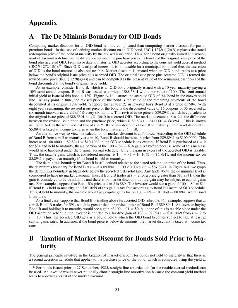
Appendix

A The De Minimis Boundary for OID BondsComputing market discount for an OID bond is more complicated than computing market discount for par orpremium bonds. In the case of defining market discount on an OID bond, IRC § 1278(a)(2)(B) replaces the statedredemption price of the bond at maturity by the revised issue price. Thus, for a bond originally issued at discount,market discount is defined as the difference between the purchase price of a bond and the original issue price of thebond plus accreted OID. From issue date to maturity, OID accretes according to the constant yield accrual method(IRC § 1272-1(b)).29 Since OID is original interest, it is not taxable for a municipal bond, and thus the accretionof OID as the bond matures is also not taxable. Market discount is created when an OID bond trades at a pricebelow the bond’s original issue price plus accreted OID. The original issue price plus accreted OID is termed therevised issue price (IRC § 1278(a)(4)) and can be computed as the present value of the remaining cashflows of thebond discounted at the bond’s original issue yield.

As an example, consider Bond B, which is an OID bond originally issued with a 10-year maturity paying a10% semi-annual coupon. Bond B was issued at a price of $88.5301 with a par value of 100. The semi-annualinitial yield at issue of this bond is 12%. Figure A-1 illustrates the accreted OID of this bond in the convex solidline. At any point in time, the revised price of the bond is the value of the remaining payments of the bonddiscounted at its original 12% yield. Suppose that at year 2, an investor buys Bond B at a price of $84. Witheight years remaining, the revised issue price of the bond is the discounted value of 16 coupons of $5 received atsix-month intervals at a yield of 6% every six months. This revised issue price is $89.8941, which is equivalent tothe original issue price of $88.5301 plus $1.3640 in accreted OID. The market discount at t = 2 is the differencebetween the revised issue price and the purchase price, which is 89.8941 − 84.0000 = $5.8941. This is shownin Figure A-1 as the solid vertical line at t = 2. If the investor holds Bond B to maturity, the market discount of$5.8941 is taxed at income tax rates when the bond matures at t = 10.

An alternative way to view the calculation of market discount is as follows. According to the OID scheduleof Bond B from t = 2 to maturity at t = 10, Bond B should increase in price from $89.8941 to $100.0000. Thisincrease of 100.0000 − 89.8941 = $10.1059 in the OID schedule is tax exempt. If Bond B is purchased at t = 2for $84 and held to maturity, then a portion of the 100 − 84 = $16 gain is tax-free because some of this increasewould have happened under the original accrual schedule. Only the gain in excess of the accreted OID is taxable.Thus, the taxable gain, which is considered income, is 100 − 84 − 10.1059 = $5.8941, and the income tax on$5.8941 is payable at maturity if the bond is held to maturity.

The de minimis boundary for Bond B is still defined relative to the stated redemption price of the bond. Thus,the de minimis boundary for Bond B at t = 2 is 89.8941−100×0.0025×8 = $87.8941. In Figure A-1, we graphthe de minimis boundary in black dots below the accreted OID solid line. Any trade above the de minimis level isconsidered to have no market discount. Thus, if Bond B trades at t = 2 for a price greater than $87.8941, then thegain is considered to be de minimis and there is no market discount, but the gain may be subject to capital gainstax. For example, suppose that Bond B’s price at t = 2 is $89. The investor would see a gain of 100 − 89 = $11if Bond B is held to maturity, and $10.1059 of this gain is tax-free according to Bond B’s accreted OID schedule.Thus, if held to maturity, the investor would pay capital gains tax on 100 − 89 − 10.1059 = $0.8941 when BondB matures.

As a final case, suppose that Bond B is trading above its accreted OID schedule. For example, suppose that att = 2, Bond B trades for $91, which is greater than the revised price of Bond B of $89.8941. An investor buyingBond B and holding it to maturity would see a gain of 100 − 91 = $9, but none of this is taxable since under theOID accretion schedule, the investor is entitled to a tax-free gain of 100 − 89.8941 = $10.1059 from t = 2 tot = 10. Thus, the accreted OID acts as a bound below which the OID bond becomes subject to tax, at least atcapital gains rates. In addition, if the bond price is below de minimis, the market discount is taxed at income taxrates.

B Taxation of Market Discount for Bonds Sold Prior to Ma-turity

The general principle involved in the taxation of market discount for bonds not held to maturity is that there isa second accretion schedule that applies to the purchase price of the bond, which is computed using the yield at

29 For bonds issued prior to 27 September, 1985, straight line amortization (or the ratable accrual method) canbe used. An investor would never rationally choose straight line amortization because the constant yield methodleads to a slower accrual of the market discount.

31

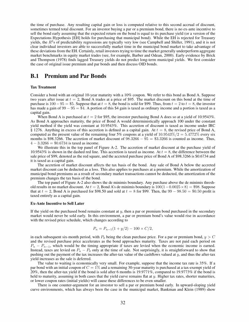
the time of purchase. Any resulting capital gain or loss is computed relative to this second accrual of discount,sometimes termed total discount. For an investor buying a par or a premium bond, there is no ex-ante incentive tosell the bond early assuming that the expected return on the bond is equal to its purchase yield (or a version of theExpectations Hypothesis [EH] holds for purchasing that municipal bond). While the EH is rejected for Treasuryyields, the R2s of predictability regressions are typically very low (see Campbell and Shiller, 1991), and it is notclear individual investors are able to successfully market time in the municipal bond market to take advantage ofthese deviations from the EH. Certainly, retail investors trying to time the market generally underperform aggregatemarket benchmarks in equity market trades (see, for example, Barber and Odean, 2000). Early evidence by Brickand Thompson (1978) finds lagged Treasury yields do not predict long-term municipal yields. We first considerthe case of original issue premium and par bonds and then discuss OID bonds.

B.1 Premium and Par Bonds

Tax Treatment

Consider a bond with an original 10-year maturity with a 10% coupon. We refer to this bond as Bond A. Supposetwo years after issue at t = 2, Bond A trades at a price of $95. The market discount on this bond at the time ofpurchase is 100− 95 = $5. Suppose that at t = 8, the bond is sold for $99. Thus, from t = 2 to t = 8, the investorhas made a gain of 99− 95 = $4. A portion of this $4 gain is taxed as ordinary income and a portion is taxed as acapital gain.

When Bond A is purchased at t = 2 for $95, the investor purchasing Bond A does so at a yield of 10.9543%.As Bond A approaches maturity, the price of Bond A would deterministically approach 100 under the constantyield method if the yield was constant at 10.9543%. This accretion of discount is taxed as income under IRC§ 1276. Anything in excess of this accretion is defined as a capital gain. At t = 8, the revised price of Bond A,computed as the present value of the remaining four 5% coupons at a yield of 10.9543%/2 = 5.4772% every sixmonths is $98.3266. The accretion of market discount of 98.3266 − 95 = $3.3266 is counted as income. Thus,4− 3.3266 = $0.6734 is taxed as income.

We illustrate this in the top panel of Figure A-2. The accretion of market discount at the purchase yield of10.9543% is shown in the dashed red line. This accretion is taxed as income. At t = 8, the difference between thesale price of $99, denoted as the red square, and the accreted purchase price of Bond A of $98.3266 is $0.6734 andit is taxed as a capital gain.

The accretion of market discount affects the tax basis of the bond. Any sale of Bond A below the accretedmarket discount can be deducted as a loss. This also applies to purchases at a premium. While the amortization ofmunicipal bond premiums as a result of secondary market transactions cannot be deducted, the amortization of thepremium changes the tax basis of the bond.

The top panel of Figure A-2 also shows the de minimis boundary. Any purchase above the de minimis thresh-old results in no market discount. At t = 2, Bond A’s de minimis boundary is 100(1−0.0025×8) = $98. Supposethat at t = 2, Bond A is purchased for $98.50 and sold at t = 8 for $99. Then, the 99 − 98.50 = $0.50 profit istaxed entirely as a capital gain.

Ex-Ante Incentive to Sell Later

If the yield on the purchased bond remains constant at y, then a par or premium bond purchased in the secondarymarket would never be sold early. In this environment, a par or premium bond’s value would rise in accordancewith the revised price schedule, which changes according to

Pn = Pn−1(1 + y/2)− 100× C/2,

in each subsequent six-month period, with P0 being the clean purchase price. For a par or premium bond, y > Cand the revised purchase price accelerates as the bond approaches maturity. Taxes are not paid each period onPn − Pn−1, which would be the timing appropriate if taxes are levied when the economic income is earned.Instead, taxes are levied on Pn − P0 only at the time of sale. Not surprisingly, it is straightforward to show thatpushing out the payment of the tax increases the after-tax value of the cashflows valued at y, and thus the after-taxyield increases as the sale is deferred.

The value to waiting is economically very small. For example, suppose that the income tax rate is 35%. If apar bond with an initial coupon of C = 1% and a remaining 30-year maturity is purchased at a tax-exempt yield of20%, then the after-tax yield if the bond is sold after 6 months is 19.9771%, compared to 19.9773% if the bond isheld to maturity, assuming in both cases that the yield curve remains flat at y. Higher tax rates, shorter maturities,or lower coupon rates (initial yields) will cause these differences to be even smaller.

There is one counter-argument for an investor to sell a par or premium bond early. In upward-sloping yieldcurve environments, which has always been the case in the municipal market, Bankman and Klein (1989) show

32

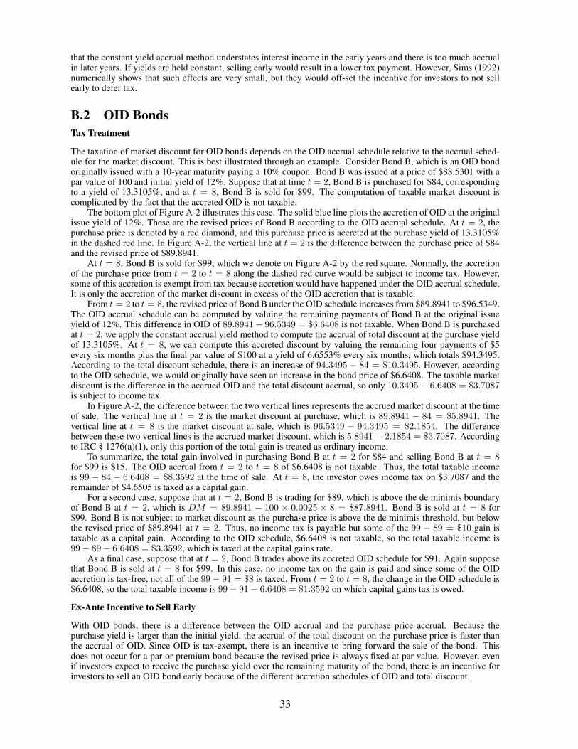
that the constant yield accrual method understates interest income in the early years and there is too much accrualin later years. If yields are held constant, selling early would result in a lower tax payment. However, Sims (1992)numerically shows that such effects are very small, but they would off-set the incentive for investors to not sellearly to defer tax.

B.2 OID BondsTax Treatment

The taxation of market discount for OID bonds depends on the OID accrual schedule relative to the accrual sched-ule for the market discount. This is best illustrated through an example. Consider Bond B, which is an OID bondoriginally issued with a 10-year maturity paying a 10% coupon. Bond B was issued at a price of $88.5301 with apar value of 100 and initial yield of 12%. Suppose that at time t = 2, Bond B is purchased for $84, correspondingto a yield of 13.3105%, and at t = 8, Bond B is sold for $99. The computation of taxable market discount iscomplicated by the fact that the accreted OID is not taxable.

The bottom plot of Figure A-2 illustrates this case. The solid blue line plots the accretion of OID at the originalissue yield of 12%. These are the revised prices of Bond B according to the OID accrual schedule. At t = 2, thepurchase price is denoted by a red diamond, and this purchase price is accreted at the purchase yield of 13.3105%in the dashed red line. In Figure A-2, the vertical line at t = 2 is the difference between the purchase price of $84and the revised price of $89.8941.

At t = 8, Bond B is sold for $99, which we denote on Figure A-2 by the red square. Normally, the accretionof the purchase price from t = 2 to t = 8 along the dashed red curve would be subject to income tax. However,some of this accretion is exempt from tax because accretion would have happened under the OID accrual schedule.It is only the accretion of the market discount in excess of the OID accretion that is taxable.

From t = 2 to t = 8, the revised price of Bond B under the OID schedule increases from $89.8941 to $96.5349.The OID accrual schedule can be computed by valuing the remaining payments of Bond B at the original issueyield of 12%. This difference in OID of 89.8941− 96.5349 = $6.6408 is not taxable. When Bond B is purchasedat t = 2, we apply the constant accrual yield method to compute the accrual of total discount at the purchase yieldof 13.3105%. At t = 8, we can compute this accreted discount by valuing the remaining four payments of $5every six months plus the final par value of $100 at a yield of 6.6553% every six months, which totals $94.3495.According to the total discount schedule, there is an increase of 94.3495 − 84 = $10.3495. However, accordingto the OID schedule, we would originally have seen an increase in the bond price of $6.6408. The taxable marketdiscount is the difference in the accrued OID and the total discount accrual, so only 10.3495− 6.6408 = $3.7087is subject to income tax.

In Figure A-2, the difference between the two vertical lines represents the accrued market discount at the timeof sale. The vertical line at t = 2 is the market discount at purchase, which is 89.8941 − 84 = $5.8941. Thevertical line at t = 8 is the market discount at sale, which is 96.5349 − 94.3495 = $2.1854. The differencebetween these two vertical lines is the accrued market discount, which is 5.8941− 2.1854 = $3.7087. Accordingto IRC § 1276(a)(1), only this portion of the total gain is treated as ordinary income.

To summarize, the total gain involved in purchasing Bond B at t = 2 for $84 and selling Bond B at t = 8for $99 is $15. The OID accrual from t = 2 to t = 8 of $6.6408 is not taxable. Thus, the total taxable incomeis 99 − 84 − 6.6408 = $8.3592 at the time of sale. At t = 8, the investor owes income tax on $3.7087 and theremainder of $4.6505 is taxed as a capital gain.

For a second case, suppose that at t = 2, Bond B is trading for $89, which is above the de minimis boundaryof Bond B at t = 2, which is DM = 89.8941 − 100 × 0.0025 × 8 = $87.8941. Bond B is sold at t = 8 for$99. Bond B is not subject to market discount as the purchase price is above the de minimis threshold, but belowthe revised price of $89.8941 at t = 2. Thus, no income tax is payable but some of the 99 − 89 = $10 gain istaxable as a capital gain. According to the OID schedule, $6.6408 is not taxable, so the total taxable income is99− 89− 6.6408 = $3.3592, which is taxed at the capital gains rate.

As a final case, suppose that at t = 2, Bond B trades above its accreted OID schedule for $91. Again supposethat Bond B is sold at t = 8 for $99. In this case, no income tax on the gain is paid and since some of the OIDaccretion is tax-free, not all of the 99− 91 = $8 is taxed. From t = 2 to t = 8, the change in the OID schedule is$6.6408, so the total taxable income is 99− 91− 6.6408 = $1.3592 on which capital gains tax is owed.

Ex-Ante Incentive to Sell Early

With OID bonds, there is a difference between the OID accrual and the purchase price accrual. Because thepurchase yield is larger than the initial yield, the accrual of the total discount on the purchase price is faster thanthe accrual of OID. Since OID is tax-exempt, there is an incentive to bring forward the sale of the bond. Thisdoes not occur for a par or premium bond because the revised price is always fixed at par value. However, evenif investors expect to receive the purchase yield over the remaining maturity of the bond, there is an incentive forinvestors to sell an OID bond early because of the different accretion schedules of OID and total discount.

33

For realistic cases, the additional advantage of selling early is worth less than 1 basis point. Consider an OIDbond with original coupon rate 2.35% with an original issue yield of 5% and a remaining maturity of 10 years.We assume the tax-exempt yield curve is flat at 6% and remains constant. If the income tax rate is 0.396, then theafter-tax yield assuming a sale in six months is 5.6971% compared to 5.6954% if the investor holds the bond to thefull 10-year maturity.

C Data FiltersFrom January 1995 to April 2007, the original MSRB database contains 70,611,395 individual transactions on2,080,291 unique municipal bonds. Our final sample consists of 6,753,847 trades on 294,442 unique securities.

1. Tax StatusWe consider only bonds that are exempt from federal and state income taxes. Some tax-exempt municipalbonds issued by state and local governments to finance capital projects are classified as private activitybonds and are subject to the AMT. These bonds comprise 3.33% of all CUSIPS and we exclude thesebonds from our analysis. We also limit our bond universe to bonds issued in one of the 50 states, and sowe exclude bonds issued in Puerto Rico, the Virgin Islands, other territories of the U.S. such as AmericanSamoa, the Canal Zone, and Guam. Bonds issued in these territories constitute less than 0.37% of all bonds.

2. High Credit RatingsTo focus only on the tax implications of municipal bond trades, we focus on bonds of the highest creditclasses. We take only bonds rated by S&P in the AAA, AA+, AA, AA-, A+, A, and A- categories. Many AGrade bonds obtain their credit rating because they are insured by a AAA-rated insurer. Slightly over 60%of all bonds are insured in the MSRB sample.30 Our S&P rating is collected at two points in time May2006 for transactions before November 2005 and July 2007 for the remainder. The S&P rating is relevantat the time of maturity for bonds that have expired, or or for current outstanding bonds at those two dates.31

3. Straight BondsWe further limit our sample to include only bonds paying fixed coupon rates (94.1% of all bonds in theMSRB sample). We also take only straight bonds with no embedded option features, so all our bonds arefixed maturity paying fixed semi-annual coupons. Straight municipal bonds constitute 50.35% of all thebond universe and they generally have shorter maturities than bonds with embedded options. The averagematurity at issue of straight bonds is 6.25 years while the average maturity at issue of option-embeddedbonds is 15.75 years. The exclusion of option-embedded bonds is to facilitate our computation of yield-to-maturity and market discounts. Including bonds with callable or sinking bond features would entailnumerically intensive option-adjusted spread computations involving binomial trees to correctly price theembedded options.After these first three requirements, we have transactions on 15,821,095 transactions on 604,118 uniquemunicipal bonds.

4. Avoiding Newly Issued BondsGreen, Hollifield and Schürhoff (2007b) document significant underpricing in new municipal bond issuesand interesting patterns in the aftermarket trading of these bonds between informed and uninformed cus-tomers. To avoid the effect of newly issued bonds, we exclude all the transactions that happened within30 days of issuance. Transaction of newly issued bonds constitute about 25.9% of the 15.8 million trans-actions, reflecting the fact that municipal bonds transactions are concentrated during the period right afterissuance. However, almost all of these transactions are not trades near de minimis because there is littlemovement in the yield curve over a 30 day period. We obtain nearly identical results when these trades areincluded in our sample.

30 Nanda and Singh (2004) provide a tax-based rationale of how insurance on municipal bonds is value-enhancingfor both insurers and municipal bond investors.

31 Unfortunately, neither S&P’s Ratings IQuery or Moody’s Ratings Delivery Service provide complete historicalrating information for public finance issues. Both these companies only provide past ratings changes for bonds thatthey currently cover. That is, for bonds that have defaulted, matured, or are no longer covered by analysts at S&Por Moody’s, past rating information on these individual bonds cannot be directly obtained from these companies.However, S&P and Moody’s do publish aggregate historical information on the default experience and transitionsbetween each credit class.

34

5. Maturities Between One and Ten YearsTransactions involving straight bonds with maturities longer than 10 years are scarce because most bondswith long maturities are issued with callable or sinking fund provisions. We use only transactions withmaturity shorter than 10 years in our analysis. We also take bonds only with maturities greater than oneyear because long-term capital gains rates apply only to securities held longer than one year and there is nomarket discount for bonds with a maturity less than one year.

6. Removing Very Small Trades and OutliersTo avoid the effect of extremely small trades, we exclude all transactions with par amounts traded less than$10,000. Finally, we take only transactions with prices between $80 and $130, and bonds with coupon ratesfrom 1% to 20%.

D Municipal Zero-Coupon Bond CurvesWe follow the method of Nelson and Siegel (1987), so the zero-coupon yield for maturity n half-years, rn, is givenby:

rn = β0 + (β1 + β2)1− exp(−n/τ)

n/τ− β2 exp(−n/τ), (D-1)

which is determined by the parameters θ = {β0, β1, β2, τ}. We estimate these parameters daily by fitting theNelson-Siegel curve to only interdealer trades traded each business day. We use only interdealer trades as they arethe trade type reported continuously over the sample (retail trades only are reported from August 1998) and repre-sent a mid-point between sales to customers or purchases from customers made by dealers. Thus, the interdealertrades avoid any distortions from transactions spreads between dealers and customers. We also take only trades ofbonds above revised price as these are fully tax-exempt municipal bonds. We also follow the same data screens asAppendix C, in particular removing any small trades below $10,000.

For each transaction price, we use the zero-coupon rate implied by equation (D-1) to discount the cashflowsof the bonds. This gives us a fitted price for each bond, Pm, which we compute by:

Pm =N∑

n=1

100× C/2(1 + rn/2)n−1+w

+100

(1 + rN/2)N−1+w− A

360100× C, (D-2)

where each cashflow is discounted by the zero-coupon yield. We denote bond prices computed using the fitted zeroyield curve as “model-implied” (or “zero-implied”) bond prices Pm with corresponding “model-implied” yieldsY m. By definition, Y m is the yield implied by valuing the bond cashflows using the municipal zero-coupon yieldcurve on that trading day.

Each trading day, we estimate the parameters θ to minimize the distance between actual transaction prices andthe predicted prices using the zero curve:

minθ

∑

i

(Pmi − Pi)2, (D-3)

where Pmi is the price of bond i computed using the Nelson-Siegel zero-coupon curve in equation (D-2) and Pi is

the transaction price of bond i in data. We take the summation over all bonds traded each day in our sample.32 Wefind that the differences between actual yields and zero-implied yields are very small, with the average differencebetween transactions yields and zero-implied yields over all bonds for our sample being 2 basis points.

Figure A-3 plots the time series of our estimated municipal zero-coupon curves for maturities of one, five, and10 years in the top two panels and the bottom left panel. Along with our estimates, we also plot the zero-couponcurve for municipal bonds from Bloomberg, which start in August 2001. Bloomberg’s method of computing zerorate curves is not made public, but Bloomberg’s sample includes bonds with callable and sinking fund features.Bloomberg’s estimation sample also relies on dealer quotations in addition to using transaction prices. Our zero-coupon rates are slightly lower than the Bloomberg data, which is expected because our sample excludes all bondswith embedded option features. Yields at the 1-year maturity hovered around 1% from 1995 to 1999, and roseto 5% in 2000 before declining to 1% in 2003. At the end of our sample in November 2005, the 1-year zeromunicipal yield was around 3%. At the long end of the yield curve, 10-year zero yields have been much morestable, generally around 4-5% over 1995 to 2007. These trends mirror the movements in Treasury yields.

In the lower right panel of Figure A-3, we plot the average term structure of municipal zero-coupon rates overour sample from one to 10 years. It is a well-known stylized fact that municipal yield curves have always been

32 In our estimations of the zero curve, there are some bonds that trade more than once per day. For these bonds,there will be more than one trading price per day, but there is only one zero-curve implied model price.

35

upward sloping (see Fabozzi and Feldstein, 1983). We find our estimated zero yield curves are upward sloping inevery trading day. The average term spread between one- and 10-year zero-coupon yields is 1.27%. To comparethis number to par coupon yields, we also plot the average par coupon yield curve implied from our zero yields.The corresponding par yield spread is 1.18%.

36

References[1] Auerbach, A. J., and M. A. King, 1983, “Taxation, Portfolio Choice, and Debt-Equity Ratios: A General

Equilibrium Model,” Quarterly Journal of Economics, 98, 587-609.

[2] Bankman, J., and W. A. Klein, 1989, “Accurate Taxation of Long-Term Debt: Taking into Account the TermStructure of Interest,” NYU Tax Law Review, 44, 335-348.

[3] Barber, B., and T. Odean, 2000, “Trading is Hazardous to Your Wealth: The Common Stock InvestmentPerformance of Individual Investors,” Journal of Finance, 55, 773-806.

[4] Bergstresser, D., and J. Poterba, 2002, “Do After-Tax Returns Affect Mutual Fund Inflows?” Journal ofFinancial Economics, 63, 381-414.

[5] Bernheim, B. D., 2002, “Taxation and Saving,” in in A. J. Auerbach and M. Feldstein, eds., Handbook ofPublic Economics Volume 3, Elsevier Science B.V., 1173-1249.

[6] Biais, B., and R. C. Green, 2005, “The Microstructure of the Bond Market in the 20th Century,” workingpaper, Carnegie Mellon University.

[7] Boyd, J. H., and R. Jagannathan, 1994, “Ex-Dividend Price Behavior of Common Stocks,” Review of Finan-cial Studies, 7, 711-741.

[8] Brick, J. R., and H. E. Thompson, 1978, “Time Series Analysis of Interest Rates: Some Additional Evidence,”Journal of Finance, 33, 93-103.

[9] Campbell, J. Y., and R. J. Shiller, 1991, “Yield Spreads and Interest Rate Movements: A BirdŠs Eye View,Review of Economic Studies,” 58, 495-514.

[10] Chalmers, J. M. R., 1998, “Default Risk Cannot Explain the Muni Puzzle: Evidence from Municipal Bondsthat are Secured by U.S. Treasury Obligations,” Review of Financial Studies, 11, 281-308.

[11] Chalmers, J. M. R., 2000, “The Muni Puzzle: Explanations and Implications for Investors,” in Jegadeesh, N.,and B. Tuckman, ed., Advanced Fixed-Income Valuation Tools, John Wiley and Sons, 302-319.

[12] Cole, C. S., P. Liu, and S. D. Smith, 1994, “The Capitalization of the State Tax Exemption Benefit in Munic-ipal Bond Yields,” Journal of Financial and Strategic Decisions, 7, 67-77.

[13] Constantinides, G. M., and J. E. Ingersoll, 1984, “Optimal Bond Trading with Personal Taxes,” Journal ofFinancial Economics, 13, 299-355.

[14] Dammon, R., and R. Green, 1987, “Tax Arbitrage and the Existence of Equilibrium Prices for FinancialAssets,” Journal of Finance, 42, 1143-1166.

[15] Downing, C. and F. Zhang, 2004, “Trading Activity and Price Volatility in the Municipal Bond Market,”Journal of Finance, 59, 899-931.

[16] Dybvig, P., and S. Ross, 1986, “Tax Clienteles and Asset Pricing,” Journal of Finance, 41, 751-763.

[17] Erickson, M., and E. L. Maydew, 1998, “Implicit Taxes in High Dividend Yield Stocks,” The AccountingReview, 73, 435-458.

[18] Erickson, M., A. Goolsbee, and E. Maydew, 2003, “How Prevalent is Tax Arbitrage? Evidence from theMarket for Municipal Bonds,” National Tax Journal, 56, 259-270.

[19] Fabozzi, F., and S. Feldstein, 1983, “Municipal Bonds,” in F. Fabozzi and T. M. Pollack, eds., Handbook ofFixed Income Securities, Dow Jones-Irwin, Homewood, IL.

[20] Fama, E. F., and K. R. French, 1998, “Taxes, Financing Decisions, and Firm Value,” Journal of Finance, 53,819-843.

[21] Fennell, C. C., and L. A. Fennell, 2003, “Fear and Greed in Tax Policy: A Qualitative Research Agenda,”Law and Economics Working Paper No. 1, University of Texas School of Law.

[22] Fama, E. F., and J. D. MacBeth, 1973, “Risk, Return, and Equilibrium: Empirical Tests,” Journal of PoliticalEconomy, 71, 607-636.

[23] Fortune, P., 1996, “Do Municipal Bond Yields Forecast Tax Policy?” New England Economic Review,Sep/Oct, 29-48.

[24] Green, R. C., 1993, “A Simple Model of the Taxable and Tax-Exempt Yield Curves,” Review of FinancialStudies, 6, 233-264.

37

[25] Green, R. C., and B. A. Ødegaard, 1997, “Are There Tax Effects in the Relative Pricing of U.S. GovernmentBonds?” Journal of Finance, 52, 609-633.

[26] Green, R. C., B. Hollifield, and N. Schürhoff, 2007a, “Financial Intermediation and Costs of Trading in anOpaque Market,” Review of Financial Studies, 20, 275-314.

[27] Green, R. C., B. Hollifield, and N. Schürhoff, 2007b, “Dealer Intermediation and Price Behavior in theAftermarket for New Bond Issues,” Journal of Financial Economics, 86, 643-682.

[28] Harris, L. E., and M. S. Piwowar, 2006, “Secondary Trading Costs in the Municipal Bond Market,” Journalof Finance, 61, 1361-97.

[29] Hong, G., and A. Warga, 2004, “Municipal Marketability,” Journal of Fixed Income, September, 86-95.

[30] Li, D., 2006, “Agreeing on a Higher Price,” working paper, Federal Reserve Board.

[31] Litvack, D., and F. Rizzo, 2000, “Municipal Default Risk,” Municipal Finance Journal, 21, 25-42.

[32] Litzenberger, R. H., and J. Rolfo, 1984, “Arbitrage Pricing, Transactions Costs and Taxation of Capital Gains:A Study of Government Bonds with the Same Maturity Date,” Journal of Financial Economics, 13, 337-351.

[33] Liu, S., J. Shi, J. Wang, and C. Wu, 2007, “How Much of the Corporate Bond Spread is due to PersonalTaxes?” Journal of Financial Economics, 85, 599-636.

[34] McCaffery, E. J., 1994, “Cognitive Theory and Tax,” UCLA Law Review, 41, 1861-1947.

[35] McDonald, R. L., 1983, “Government Debt and Private Leverage,” Journal of Public Economics, 22, 303-325.

[36] Nanda, V., and R. Singh, 2004, “Bond Insurance: What is Special about Munis?” Journal of Finance, 59,2253-79.

[37] Nelson, C. R., and A. F. Siegel, 1987, “Parsimonious Modeling of Yield Curves,” Journal of Business, 60,473-489.

[38] Poterba, J. M., 2002, “Taxation, Risk-Taking, and Household Portfolio Behavior,” in A. J. Auerbach and M.Feldstein, eds., Handbook of Public Economics Volume 3, Elsevier Science B.V., 1110-71.

[39] Sims, T. S., 1992, “Long-Term Debt, the Term Structure of Interest and the Case for Accrual Taxation,” NYUTax Law Review, 47, 313-375.

[40] Strnad, J., 1995, “The Taxation of Bonds: The Tax Trading Dimension,” Virginia Law Review, 81, 47-116.

[41] Sullivan, M., 2007, “The Effective Corporate Tax Rate is Falling,” Tax Analysts Tax Notes, Jan 22, 2007.

[42] Woodell, C., W. Montrone, and B. Brady, 2004, “U.S. Municipal Rating Transitions and Defaults, 1986-2003,” Municipal Finance Journal, 24, 49-78.

38

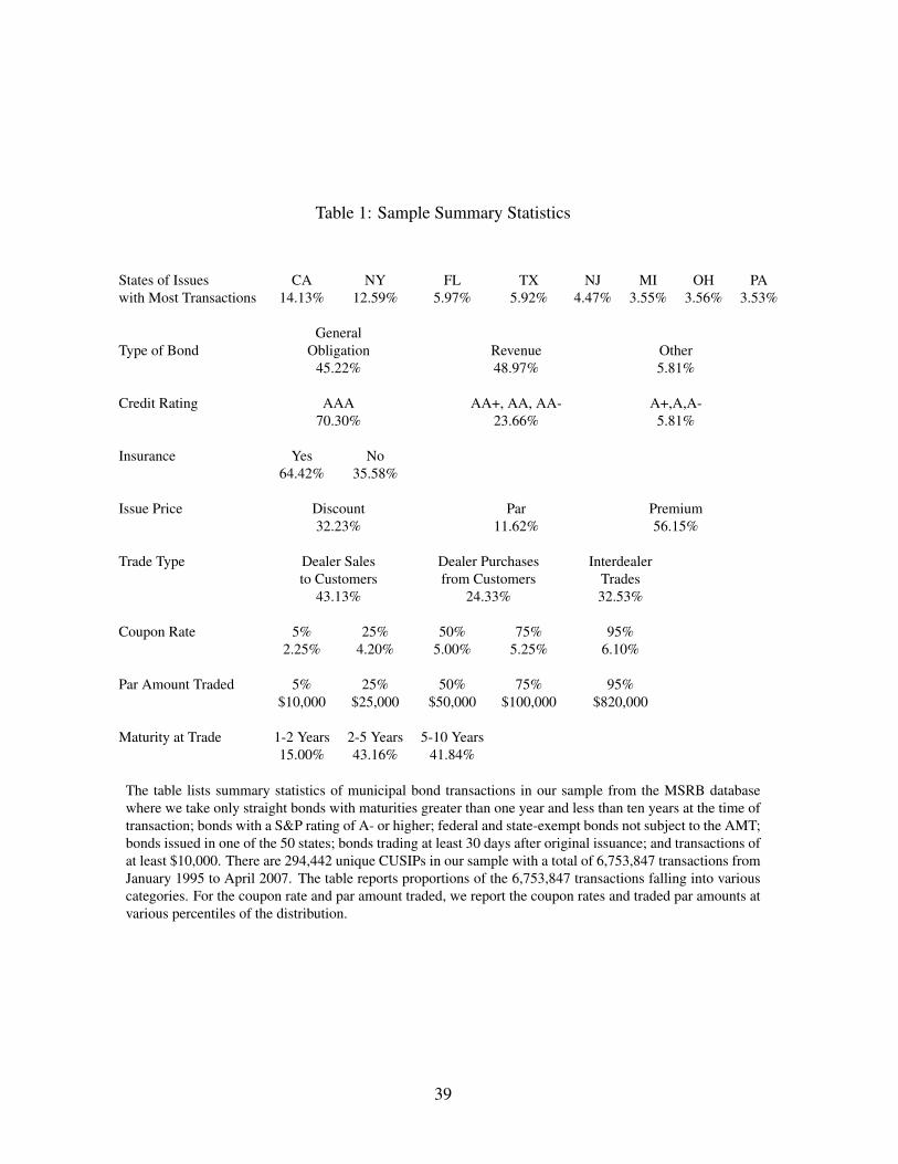
Table 1: Sample Summary Statistics

States of Issues CA NY FL TX NJ MI OH PAwith Most Transactions 14.13% 12.59% 5.97% 5.92% 4.47% 3.55% 3.56% 3.53%

GeneralType of Bond Obligation Revenue Other

45.22% 48.97% 5.81%

Credit Rating AAA AA+, AA, AA- A+,A,A-70.30% 23.66% 5.81%

Insurance Yes No64.42% 35.58%

Issue Price Discount Par Premium32.23% 11.62% 56.15%

Trade Type Dealer Sales Dealer Purchases Interdealerto Customers from Customers Trades

43.13% 24.33% 32.53%

Coupon Rate 5% 25% 50% 75% 95%2.25% 4.20% 5.00% 5.25% 6.10%

Par Amount Traded 5% 25% 50% 75% 95%$10,000 $25,000 $50,000 $100,000 $820,000

Maturity at Trade 1-2 Years 2-5 Years 5-10 Years15.00% 43.16% 41.84%

The table lists summary statistics of municipal bond transactions in our sample from the MSRB databasewhere we take only straight bonds with maturities greater than one year and less than ten years at the time oftransaction; bonds with a S&P rating of A- or higher; federal and state-exempt bonds not subject to the AMT;bonds issued in one of the 50 states; bonds trading at least 30 days after original issuance; and transactions ofat least $10,000. There are 294,442 unique CUSIPs in our sample with a total of 6,753,847 transactions fromJanuary 1995 to April 2007. The table reports proportions of the 6,753,847 transactions falling into variouscategories. For the coupon rate and par amount traded, we report the coupon rates and traded par amounts atvarious percentiles of the distribution.

39

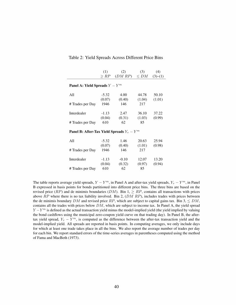
Table 2: Yield Spreads Across Different Price Bins

(1) (2) (3) (4)≥ RP (DM RP ) ≤ DM (3)–(1)

Panel A: Yield Spreads Y − Y m

All -5.32 4.00 44.78 50.10(0.07) (0.40) (1.04) (1.01)

# Trades per Day 1946 146 217

Interdealer -1.13 2.47 36.10 37.22(0.04) (0.31) (1.03) (0.99)

# Trades per Day 610 62 85

Panel B: After-Tax Yield Spreads Yτ − Y m

All -5.32 1.46 20.63 25.94(0.07) (0.40) (1.01) (0.98)

# Trades per Day 1946 146 217

Interdealer -1.13 -0.10 12.07 13.20(0.04) (0.32) (0.97) (0.94)

# Trades per Day 610 62 85

The table reports average yield spreads, Y − Y m, in Panel A and after-tax yield spreads, Yτ − Y m, in PanelB expressed in basis points for bonds partitioned into different price bins. The three bins are based on therevised price (RP ) and de minimis boundaries (DM ). Bin 1, ≥ RP , contains all transactions with pricesabove RP where there is no tax liability involved. Bin 2, (DM RP ), includes trades with prices betweenthe de minimis boundary DM and revised price RP , which are subject to capital gains tax. Bin 3, ≤ DM ,contains all the trades with prices below DM , which are subject to income tax. In Panel A, the yield spreadY −Y m is defined as the actual transaction yield minus the model-implied yield (the yield implied by valuingthe bond cashflows using the municipal zero-coupon yield curve on that trading day). In Panel B, the after-tax yield spread, Yτ − Y m, is computed as the difference between the after-tax transaction yield and themodel-implied yield. All spreads are reported in basis points. In computing averages, we only include daysfor which at least one trade takes place in all the bins. We also report the average number of trades per dayfor each bin. We report standard errors of the time-series averages in parentheses computed using the methodof Fama and MacBeth (1973).

40

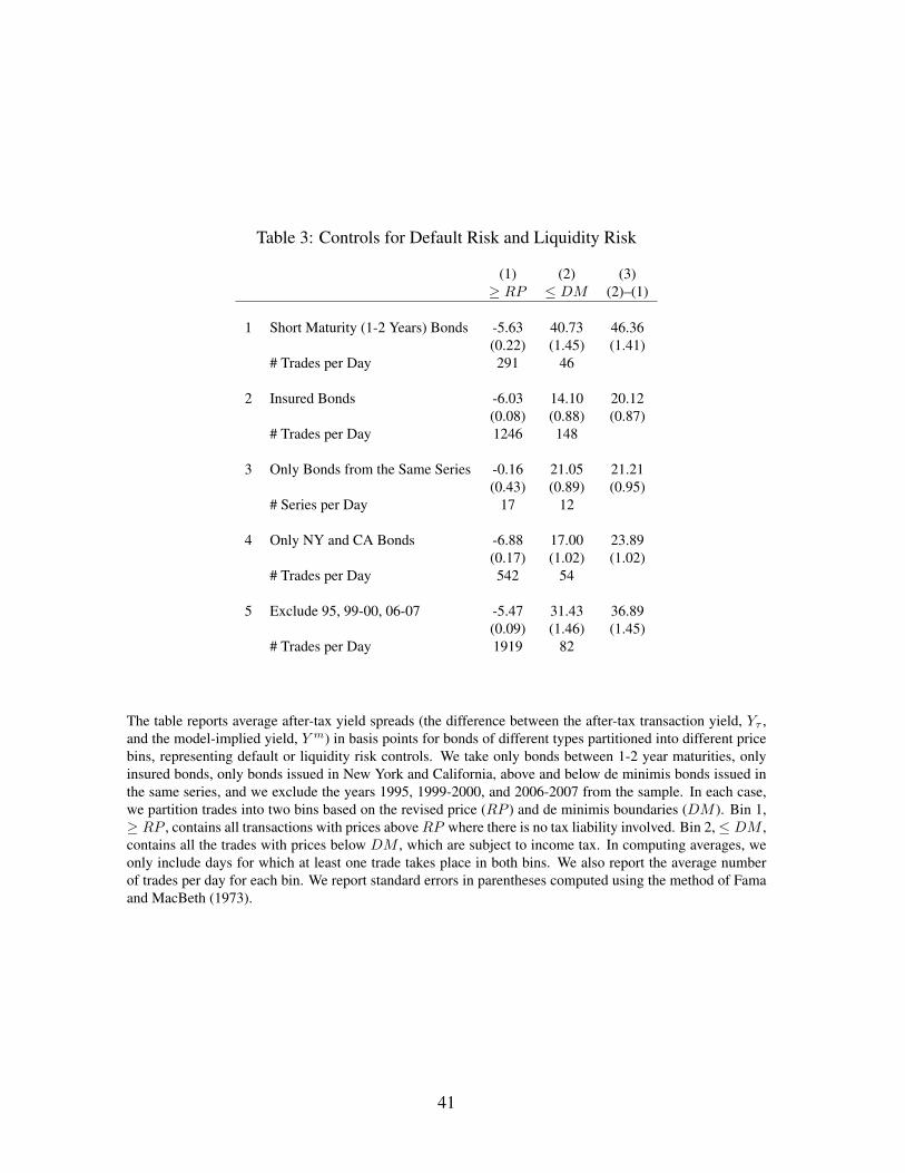
Table 3: Controls for Default Risk and Liquidity Risk

(1) (2) (3)≥ RP ≤ DM (2)–(1)

1 Short Maturity (1-2 Years) Bonds -5.63 40.73 46.36(0.22) (1.45) (1.41)

# Trades per Day 291 46

2 Insured Bonds -6.03 14.10 20.12(0.08) (0.88) (0.87)

# Trades per Day 1246 148

3 Only Bonds from the Same Series -0.16 21.05 21.21(0.43) (0.89) (0.95)

# Series per Day 17 12

4 Only NY and CA Bonds -6.88 17.00 23.89(0.17) (1.02) (1.02)

# Trades per Day 542 54

5 Exclude 95, 99-00, 06-07 -5.47 31.43 36.89(0.09) (1.46) (1.45)

# Trades per Day 1919 82

The table reports average after-tax yield spreads (the difference between the after-tax transaction yield, Yτ ,and the model-implied yield, Y m) in basis points for bonds of different types partitioned into different pricebins, representing default or liquidity risk controls. We take only bonds between 1-2 year maturities, onlyinsured bonds, only bonds issued in New York and California, above and below de minimis bonds issued inthe same series, and we exclude the years 1995, 1999-2000, and 2006-2007 from the sample. In each case,we partition trades into two bins based on the revised price (RP ) and de minimis boundaries (DM ). Bin 1,≥ RP , contains all transactions with prices above RP where there is no tax liability involved. Bin 2,≤ DM ,contains all the trades with prices below DM , which are subject to income tax. In computing averages, weonly include days for which at least one trade takes place in both bins. We also report the average numberof trades per day for each bin. We report standard errors in parentheses computed using the method of Famaand MacBeth (1973).

41

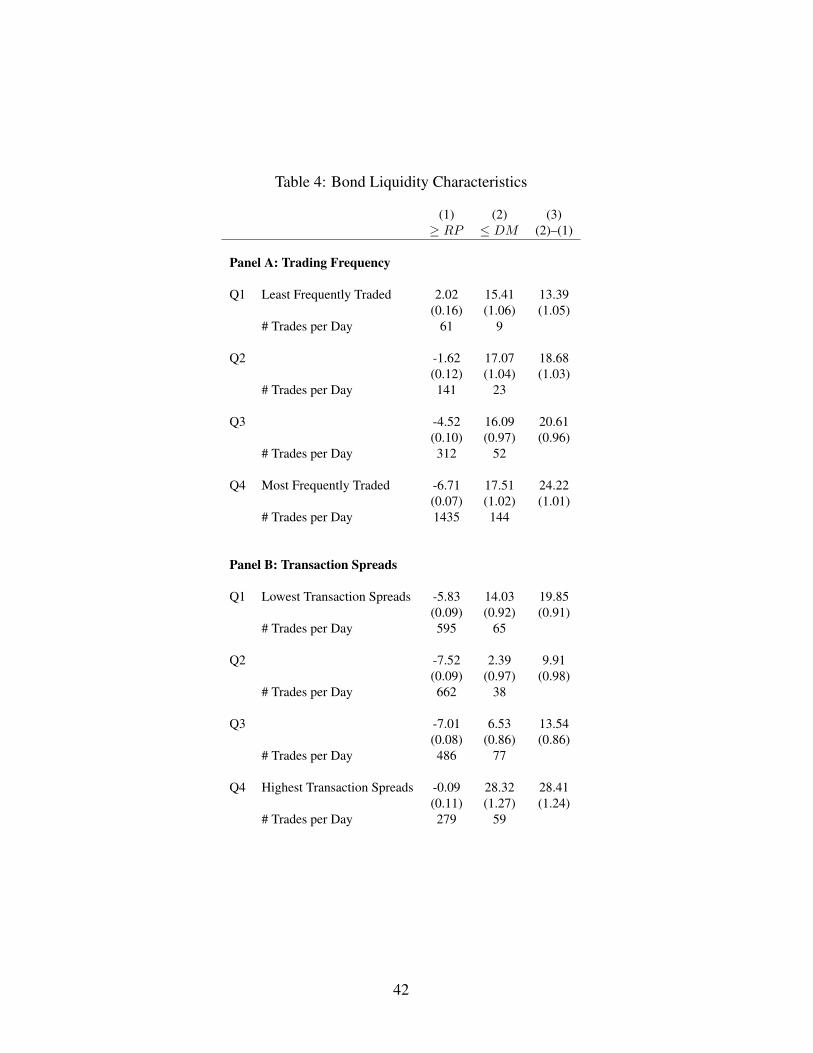
Table 4: Bond Liquidity Characteristics

(1) (2) (3)≥ RP ≤ DM (2)–(1)

Panel A: Trading Frequency

Q1 Least Frequently Traded 2.02 15.41 13.39(0.16) (1.06) (1.05)

# Trades per Day 61 9

Q2 -1.62 17.07 18.68(0.12) (1.04) (1.03)

# Trades per Day 141 23

Q3 -4.52 16.09 20.61(0.10) (0.97) (0.96)

# Trades per Day 312 52

Q4 Most Frequently Traded -6.71 17.51 24.22(0.07) (1.02) (1.01)

# Trades per Day 1435 144

Panel B: Transaction Spreads

Q1 Lowest Transaction Spreads -5.83 14.03 19.85(0.09) (0.92) (0.91)

# Trades per Day 595 65

Q2 -7.52 2.39 9.91(0.09) (0.97) (0.98)

# Trades per Day 662 38

Q3 -7.01 6.53 13.54(0.08) (0.86) (0.86)

# Trades per Day 486 77

Q4 Highest Transaction Spreads -0.09 28.32 28.41(0.11) (1.27) (1.24)

# Trades per Day 279 59

42

Note to Table 4The table reports average after-tax yield spreads (the difference between the after-tax transaction yield, Yτ ,and the model-implied yield, Y m) in basis points for bonds sorted by trading frequency and by transactionspreads. In Panel A, we record the number of trades for all bonds in our sample and rank them into quartilesby trading frequency, defined as the number of trades of each bond per annum. Then, for the bonds in eachquartile we divide transactions into above revised price and below de minimis bins and compute after-taxyield spreads, Yτ −Y m, for each quartile. The table reports the average after-tax yield spread of each quartileand bin over the sample. Panel B defines the transaction spread as the difference between dealer sales tocustomers and dealer purchases from customers. We compute transactions spreads for each day for eachbond, and then we average the transaction spreads over time. Using each bond’s average transaction spreadover the sample, we rank the bonds into quartiles and divide the transactions into the two above revised priceand below de minimis price bins. In computing averages, we only include days for which at least one tradetakes place in both bins. We also report the average number of trades per day for each bin. We report standarderrors in parentheses computed using the method of Fama and MacBeth (1973).

43

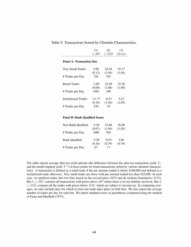
Table 5: Transactions Sorted by Clientele Characteristics

(1) (2) (3)≥ RP ≤ DM (2)–(1)

Panel A: Transaction Size

Very Small Trades 3.00 28.38 25.37(0.13) (1.04) (1.04)

# Trades per Day 744 102

Retail Trades -2.80 22.48 25.28(0.09) (1.00) (1.00)

# Trades per Day 1485 189

Institutional Trades -11.77 -6.53 5.23(0.10) (1.04) (1.05)

# Trades per Day 476 35

Panel B: Bank Qualified Issues

Non-Bank Qualified -5.29 21.68 26.98(0.07) (1.04) (1.03)

# Trades per Day 1880 204

Bank Qualified -5.58 -0.53 5.06(0.16) (0.79) (0.79)

# Trades per Day 67 17

The table reports average after-tax yield spreads (the difference between the after-tax transaction yield, Yτ ,and the model-implied yield, Y m) in basis points for bond transactions sorted by various clientele character-istics. A transaction is defined as a retail trade if the par amount traded is below $100,000 and defined as ainstitutional trade otherwise. Very small trades are those with par amount traded less than $25,000. In eachcase, we partition trades into two bins based on the revised price (RP ) and de minimis boundaries (DM ).Bin 1, ≥ RP , contains all transactions with prices above RP where there is no tax liability involved. Bin 2,≤ DM , contains all the trades with prices below DM , which are subject to income tax. In computing aver-ages, we only include days for which at least one trade takes place in both bins. We also report the averagenumber of trades per day for each bin. We report standard errors in parentheses computed using the methodof Fama and MacBeth (1973).

44

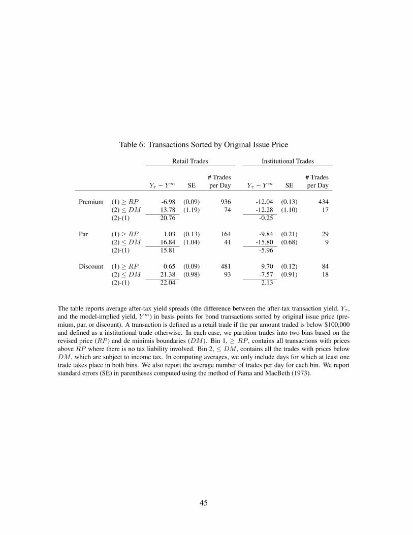
Table 6: Transactions Sorted by Original Issue Price

Retail Trades Institutional Trades

# Trades # TradesYτ − Y m SE per Day Yτ − Y m SE per Day

Premium (1) ≥ RP -6.98 (0.09) 936 -12.04 (0.13) 434(2) ≤ DM 13.78 (1.19) 74 -12.28 (1.10) 17(2)-(1) 20.76 -0.25

Par (1) ≥ RP 1.03 (0.13) 164 -9.84 (0.21) 29(2) ≤ DM 16.84 (1.04) 41 -15.80 (0.68) 9(2)-(1) 15.81 -5.96

Discount (1) ≥ RP -0.65 (0.09) 481 -9.70 (0.12) 84(2) ≤ DM 21.38 (0.98) 93 -7.57 (0.91) 18(2)-(1) 22.04 2.13

The table reports average after-tax yield spreads (the difference between the after-tax transaction yield, Yτ ,and the model-implied yield, Y m) in basis points for bond transactions sorted by original issue price (pre-mium, par, or discount). A transaction is defined as a retail trade if the par amount traded is below $100,000and defined as a institutional trade otherwise. In each case, we partition trades into two bins based on therevised price (RP ) and de minimis boundaries (DM ). Bin 1, ≥ RP , contains all transactions with pricesabove RP where there is no tax liability involved. Bin 2, ≤ DM , contains all the trades with prices belowDM , which are subject to income tax. In computing averages, we only include days for which at least onetrade takes place in both bins. We also report the average number of trades per day for each bin. We reportstandard errors (SE) in parentheses computed using the method of Fama and MacBeth (1973).

45

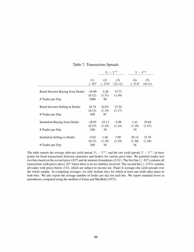
Table 7: Transactions Spreads

Yτ − Y m Y − Y m

(1) (2) (3) (4) (5)≥ RP ≤ DM (2)–(1) ≤ DM (4)-(1)

Retail Investor Buying from Dealer -18.99 -3.26 15.73(0.12) (1.51) (1.49)

# Trades per Day 1006 98

Retail Investor Selling to Dealer 18.74 42.03 23.30(0.13) (1.19) (1.17)

# Trades per Day 450 87

Institution Buying from Dealer -18.03 -23.11 -5.08 1.41 19.44(0.15) (1.24) (1.24) (1.18) (1.47)

# Trades per Day 240 10 10

Institution Selling to Dealer -5.62 1.48 7.09 28.14 33.76(0.13) (1.18) (1.19) (1.38) (1.38)

# Trades per Day 168 16 16

The table reports the average after-tax yield spread, Yτ − Y m, and the raw yield spread, Y − Y m, in basispoints for bond transactions between customers and dealers for various price bins. We partition trades intotwo bins based on the revised price (RP ) and de minimis boundaries (DM ). The first bin (≥ RP ) contains alltransactions with prices above RP where there is no tax liability involved. The second bin (≤ DM ) containsall trades with prices below DM , which are subject to income tax. Panel A averages the yield spreads overthe whole sample. In computing averages, we only include days for which at least one trade takes place inboth bins. We also report the average number of trades per day for each bin. We report standard errors inparentheses computed using the method of Fama and MacBeth (1973).

46

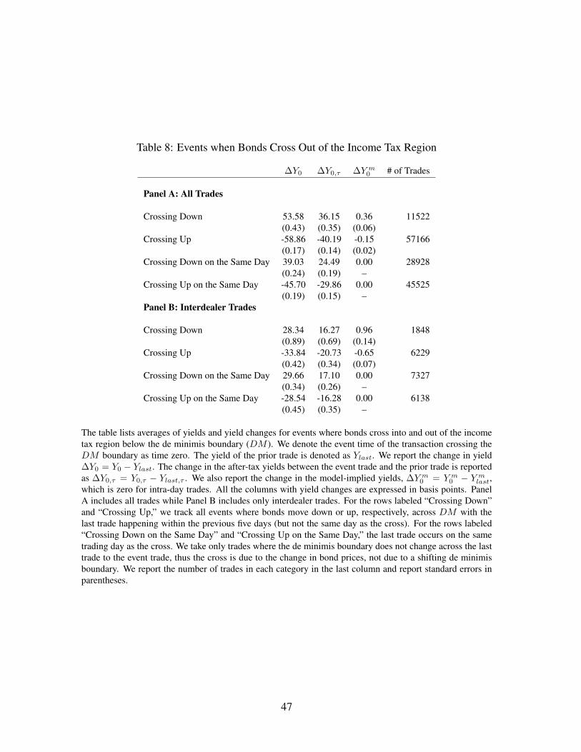
Table 8: Events when Bonds Cross Out of the Income Tax Region

∆Y0 ∆Y0,τ ∆Y m0 # of Trades

Panel A: All Trades

Crossing Down 53.58 36.15 0.36 11522(0.43) (0.35) (0.06)

Crossing Up -58.86 -40.19 -0.15 57166(0.17) (0.14) (0.02)

Crossing Down on the Same Day 39.03 24.49 0.00 28928(0.24) (0.19) –

Crossing Up on the Same Day -45.70 -29.86 0.00 45525(0.19) (0.15) –

Panel B: Interdealer Trades

Crossing Down 28.34 16.27 0.96 1848(0.89) (0.69) (0.14)

Crossing Up -33.84 -20.73 -0.65 6229(0.42) (0.34) (0.07)

Crossing Down on the Same Day 29.66 17.10 0.00 7327(0.34) (0.26) –

Crossing Up on the Same Day -28.54 -16.28 0.00 6138(0.45) (0.35) –

The table lists averages of yields and yield changes for events where bonds cross into and out of the incometax region below the de minimis boundary (DM ). We denote the event time of the transaction crossing theDM boundary as time zero. The yield of the prior trade is denoted as Ylast. We report the change in yield∆Y0 = Y0 − Ylast. The change in the after-tax yields between the event trade and the prior trade is reportedas ∆Y0,τ = Y0,τ − Ylast,τ . We also report the change in the model-implied yields, ∆Y m

0 = Y m0 − Y m

last,which is zero for intra-day trades. All the columns with yield changes are expressed in basis points. PanelA includes all trades while Panel B includes only interdealer trades. For the rows labeled “Crossing Down”and “Crossing Up,” we track all events where bonds move down or up, respectively, across DM with thelast trade happening within the previous five days (but not the same day as the cross). For the rows labeled“Crossing Down on the Same Day” and “Crossing Up on the Same Day,” the last trade occurs on the sametrading day as the cross. We take only trades where the de minimis boundary does not change across the lasttrade to the event trade, thus the cross is due to the change in bond prices, not due to a shifting de minimisboundary. We report the number of trades in each category in the last column and report standard errors inparentheses.

47

Table 9: Implicit Income Tax Rates

Full Sample Pre-2003 Post-2003

Income Income IncomeTrade Type Tax Rate T-stat Tax Rate T-stat Tax Rate T-stat

Panel A: Direct Estimates

All 0.88 39.7 1.08 38.1 0.51 15.8Interdealer 0.71 32.2 0.87 33.6 0.40 10.5Retail 0.96 43.0 1.18 42.0 0.54 16.7Institutional 0.24 12.5 0.26 11.2 0.20 6.15

Panel B: OLS Estimation

All 0.70 9.25 0.79 7.05 0.53 9.20Interdealer 0.80 9.07 0.96 6.97 0.52 18.8Retail 1.29 7.74 1.37 1.45 0.89 6.04Institutional 0.65 30.4 0.74 22.8 0.53 21.8

The table reports estimates of implicit tax rates from the prices of market discount bonds. In Panel A,we invert the estimated tax rate τI directly from equation (4). We compute estimates of τI using all marketdiscount bonds on each trading day and then report the mean and t-statistics of the daily time-series estimates.In Panel B, we treat τI as an OLS coefficient and add fixed year effects and other controls to the regressionimplied from equation (4). We use fixed effects for each year, dummies for different bond types (generalobligation or revenue), dummies for different original issue prices (par or premium), and dummies for theeight most traded states (CA, NY, FL, TX, NJ, MI, OH, and PA). Panel B reports time-series estimates of theOLS coefficient τI following Fama and MacBeth (1973). Retail trades refer to trades with par value smallerthan $100,000.

48

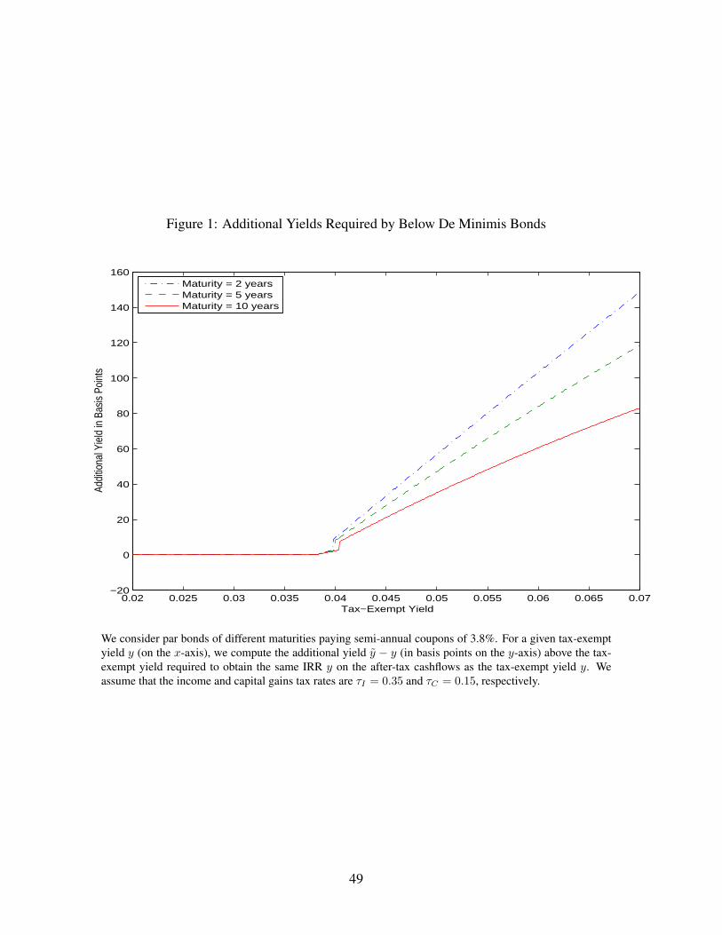
Figure 1: Additional Yields Required by Below De Minimis Bonds

0.02 0.025 0.03 0.035 0.04 0.045 0.05 0.055 0.06 0.065 0.07−20

0

20

40

60

80

100

120

140

160

Tax−Exempt Yield

Addi

tiona

l Yie

ld in

Bas

is Po

ints

Maturity = 2 yearsMaturity = 5 yearsMaturity = 10 years

We consider par bonds of different maturities paying semi-annual coupons of 3.8%. For a given tax-exemptyield y (on the x-axis), we compute the additional yield y − y (in basis points on the y-axis) above the tax-exempt yield required to obtain the same IRR y on the after-tax cashflows as the tax-exempt yield y. Weassume that the income and capital gains tax rates are τI = 0.35 and τC = 0.15, respectively.

49

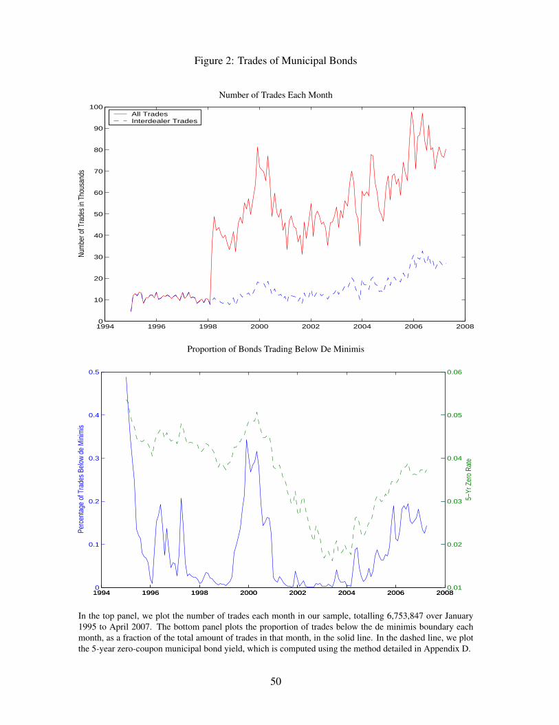
Figure 2: Trades of Municipal Bonds

Number of Trades Each Month

1994 1996 1998 2000 2002 2004 2006 20080

10

20

30

40

50

60

70

80

90

100

Num

ber o

f Tra

des

in T

hous

ands

All TradesInterdealer Trades

Proportion of Bonds Trading Below De Minimis

1994 1996 1998 2000 2002 2004 2006 20080

0.1

0.2

0.3

0.4

0.5

Perc

enta

ge o

f Tra

des

Belo

w de

Min

imis

1994 1996 1998 2000 2002 2004 2006 20080.01

0.02

0.03

0.04

0.05

0.06

5−Yr

Zer

o Ra

te

In the top panel, we plot the number of trades each month in our sample, totalling 6,753,847 over January1995 to April 2007. The bottom panel plots the proportion of trades below the de minimis boundary eachmonth, as a fraction of the total amount of trades in that month, in the solid line. In the dashed line, we plotthe 5-year zero-coupon municipal bond yield, which is computed using the method detailed in Appendix D.

50

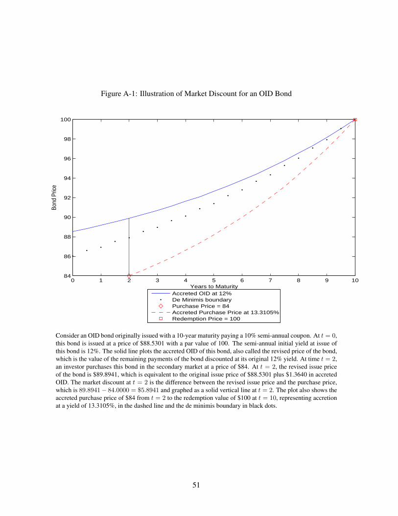
Figure A-1: Illustration of Market Discount for an OID Bond

0 1 2 3 4 5 6 7 8 9 1084

86

88

90

92

94

96

98

100

Years to Maturity

Bond

Pric

e

Accreted OID at 12%De Minimis boundaryPurchase Price = 84Accreted Purchase Price at 13.3105%Redemption Price = 100

Consider an OID bond originally issued with a 10-year maturity paying a 10% semi-annual coupon. At t = 0,this bond is issued at a price of $88.5301 with a par value of 100. The semi-annual initial yield at issue ofthis bond is 12%. The solid line plots the accreted OID of this bond, also called the revised price of the bond,which is the value of the remaining payments of the bond discounted at its original 12% yield. At time t = 2,an investor purchases this bond in the secondary market at a price of $84. At t = 2, the revised issue priceof the bond is $89.8941, which is equivalent to the original issue price of $88.5301 plus $1.3640 in accretedOID. The market discount at t = 2 is the difference between the revised issue price and the purchase price,which is 89.8941− 84.0000 = $5.8941 and graphed as a solid vertical line at t = 2. The plot also shows theaccreted purchase price of $84 from t = 2 to the redemption value of $100 at t = 10, representing accretionat a yield of 13.3105%, in the dashed line and the de minimis boundary in black dots.

51

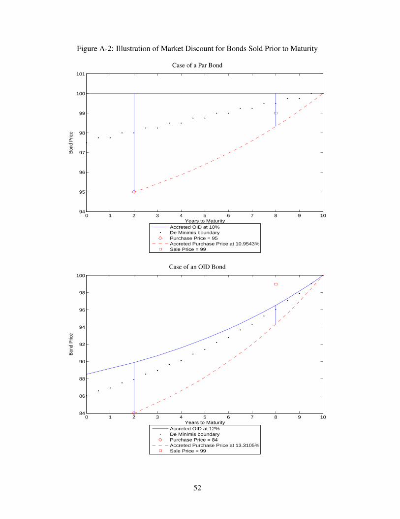
Figure A-2: Illustration of Market Discount for Bonds Sold Prior to Maturity

Case of a Par Bond

0 1 2 3 4 5 6 7 8 9 1094

95

96

97

98

99

100

101

Years to Maturity

Bond

Pric

e

Accreted OID at 10%De Minimis boundaryPurchase Price = 95Accreted Purchase Price at 10.9543%Sale Price = 99

Case of an OID Bond

0 1 2 3 4 5 6 7 8 9 1084

86

88

90

92

94

96

98

100

Years to Maturity

Bond

Pric

e

Accreted OID at 12%De Minimis boundaryPurchase Price = 84Accreted Purchase Price at 13.3105%Sale Price = 99

52

Note to Figure A-2The figure illustrates the taxation of market discount for a bond sold prior to maturity. We consider thecase of a par bond in the top panel and an OID bond in the bottom panel. In the top panel, consider a parbond originally issued with a 10-year maturity paying a 10% semi-annual coupon (Bond A). The top panelillustrates the case of a market transaction comprising both income and capital gain components. At t = 2,Bond A is sold at a price of $95 representing a yield of 10.9543%. This point is denoted as a diamond in thefigure. The dashed line plots the accreted discount of the $95 purchase price (the revised price) to maturity ata yield of 10.9543%. This accretion is taxed as income. At t = 8, the bond is sold for a price of $99, which isdenoted by a square. The revised price of Bond A at t = 8 is $98.3266. The gain in excess of the accretion ofmarket discount is the distance between the red square and the dashed line, which is $0.6734, which is taxedas a capital gain. The remaining $3.3266, which is the accretion of market discount, is taxed as income. Inthe bottom panel, consider Bond B, which is an OID bond originally issued with a 10-year maturity payinga 10% coupon. Bond B was issued at a price of $88.5301 with a par value of 100 with an initial yield of12%. The accretion of OID from t = 0 is shown in the solid blue line. Suppose that at time t = 2, BondB is purchased for $84 at a yield of 13.3105%, which is denoted by the red diamond. The accretion of thispurchase price at 13.3105% is shown in the dashed red line. At t = 8, Bond B is sold for $99, denoted in thefigure as a red square. The first vertical line at t = 2 represents the market discount at purchase. The secondvertical line at t = 8 represents the market discount at sale. The difference between the two vertical linesrepresents the accrued market discount at the time of sale, which is taxed as income at the time of sale.

53

Figure A-3: Municipal Zero-Coupon Yield Curves

1996 1998 2000 2002 2004 2006 20080

0.01

0.02

0.03

0.04

0.05

0.06

0.07

0.08

0.09

0.11 Year Zero Rate

0 2 4 6 8 100.03

0.032

0.034

0.036

0.038

0.04

0.042

0.044

0.046

0.048

0.05

Maturity in Years

Average Zero Curve and Par Yield Curve

1996 1998 2000 2002 2004 2006 20080

0.01

0.02

0.03

0.04

0.05

0.06

0.07

0.08

0.09

0.15 Year Zero Rate

1996 1998 2000 2002 2004 2006 20080

0.01

0.02

0.03

0.04

0.05

0.06

0.07

0.08

0.09

0.110 Year Zero Rate

Zero RatePar Yield

The plot displays the estimated municipal zero-coupon yield curves for our A-grade municipal bond sample.The construction method is outlined in Appendix D. In the top two plots, as well as the bottom left plot, wedisplay the estimated zero curves in solid, heavy lines for various maturities. For comparison, we overlayBloomberg’s AAA yields in the red, light lines from August 2001. In the bottom right plot, we graph theaverage zero yield curve and the average par yield curve over the January 1995 to April 2007 sample.

54