tch-13-190: supplements

TCH-13-190: Supplements

In this supplementary document, Section1 includes the derivations for the optimal so-lutions of SIS1 and SIS2 with a multivariate input vector. Sections 2 and 3 present thenumerical examples with a univariate input variable and a multivariate input vector, respec-tively, which are used to investigate the impacts of various factors on the performance ofthe proposed methods. Section 4 discusses the implementation details with the wind turbinesimulators.

1 Derivations for Optimal Stochastic Important Sam-

pling

This section details the derivations of the optimal allocation size, Ni, i = 1, 2, · · · ,M , andthe optimal IS density, qSIS1, for SIS1 and the optimal IS density, qSIS2, for SIS2, presentedin Section 3 of the paper. In the sequel, we consider a multivariate input vector, X ∈ Rp.Note that a univariate input vector is a special case with p = 1.

1.1 Optimal Important Sampling density and allocations in SIS1

First, we consider the SIS1 estimator,

P̂SIS1 =1

M

M∑i=1

P̂ (Y > l | Xi)f(Xi)

q(Xi)

=1

M

M∑i=1

(1

Ni

Ni∑j=1

I(Y

(i)j > l

)) f(Xi)

q(Xi). (S.1)

We decompose the variance of this estimator into two components, the expectation ofconditional variance and the variance of conditional expectation, as

V ar[P̂SIS1

]= V ar

[1

M

M∑i=1


q(Xi)

]

=1

M2Eq

[V ar

[M∑i=1


q(Xi)

∣∣∣∣∣ X1, · · · ,XM

]]

+1

M2V arq

[E

[M∑i=1


q(Xi)

∣∣∣∣∣ X1, · · · ,XM

]]. (S.2)

1

For simplicity, let s(X) denote the conditional POE, P (Y > l | X). Using the fact that

Xii.i.d∼ q for i = 1, 2, · · · ,M , we simplify V ar

[P̂SIS1

]in (S.2) to

V ar[P̂SIS1

]=

1

M2Eq

[V ar

[M∑i=1

(1

Ni

Ni∑j=1

I(Y

(i)j > l

)) f(Xi)

q(Xi)

∣∣∣∣∣ X1, · · · ,XM

]]

+1

M2V arq

[M∑i=1

s(Xi)f(Xi)

q(Xi)

]

=1

M2Eq

[M∑i=1

(1

N2i

Ni∑j=1

s(Xi) (1− s(Xi))

)f(Xi)

2

q(Xi)2

]+

1

MV arq

[s(X)

f(X)

q(X)

]

=1

M2Eq

[M∑i=1

1

Ni

s(Xi) (1− s(Xi))f(Xi)

2

q(Xi)2

]+

1

MV arq

[s(X)

f(X)

q(X)

]. (S.3)

We express the allocation size, Ni, at Xi as a proportion of the total simulation budget,NT ,

Ni = NT ·c(Xi)∑Mj=1 c(Xj)

, i = 1, 2, · · · ,M, (S.4)

where c(X) is a non-negative function. Lemma 1 presents the optimal assignment of simu-lation replications, Ni, to each Xi for given q.

Lemma 1 Given q, the variance in (S.3) is minimized if and only if

Ni =

√s(Xi) (1− s(Xi))f(Xi) /q(Xi)∑M

j=1

√s(Xj) (1− s(Xj))f(Xj) /q(Xj)

·NT for i = 1, 2, · · · ,M. (S.5)

Proof. We want to find Ni, i = 1, 2, · · · ,M , that minimizes the variance in (S.3) forany given function, q(X). Note that the second term in (S.3) is constant, provided that thefunction q(X) is given, and the other functions, f(X) and s(X), are fixed. Thus, we find Ni

2

that minimizes the first term in (S.3),

1

M2Eq

[M∑i=1

1

Nis(Xi) (1− s(Xi))

f(Xi)2

q(Xi)2

]

=1

M2

M∑i=1

Eq

[1

Nis(Xi) (1− s(Xi))

f(Xi)2

q(Xi)2

]

=1

MEq

[1

N1s(X1) (1− s(X1))

f(X1)2

q(X1)2

](S.6)

=1

M

1

NTEq

[∑Mj=1 c(Xj)

c(X1)s(X1) (1− s(X1))

f(X1)2

q(X1)2

](S.7)

=1

M

1

NT

M∑j=1

Eq

[c(Xj)

c(X1)s(X1) (1− s(X1))

f(X1)2

q(X1)2

]=

1

M

1

NT

Eq [s(X1) (1− s(X1))f(X1)

2

q(X1)2

]+

M∑j=2

Eq

[c(Xj)

c(X1)s(X1) (1− s(X1))

f(X1)2

q(X1)2

]=

1

M

1

NT

(Eq

[s(X) (1− s(X))

f(X)2

q(X)2

]+ (M − 1) · Eq [c(X)] · Eq

[1

c(X)s(X) (1− s(X))

f(X)2

q(X)2

])(S.8)

≥ 1

M

1

NT

(Eq

[s(X) (1− s(X))

f(X)2

q(X)2

]+ (M − 1) ·

(Eq

[√s(X) (1− s(X))

f(X)

q(X)

])2)

(S.9)

The equalities in (S.6) and (S.8) are due to the fact that Xi, i = 1, 2, · · · ,M , is independentand identically distributed. We use the definition in (S.4) for (S.7). The inequality in (S.9)follows by applying the Cauchy-Schwarz inequality to the second term in (S.8). The equalityin (S.9) holds if and only if c(X) = k

√s(X) (1− s(X))f(X) /q(X), where k is a positive

constant. Therefore, by the definition in (S.4), the optimal allocation size in (S.5) follows.�

3

Plugging Ni’s in (S.5) into the estimator variance in (S.3) leads to

V ar[P̂SIS1

]=

1

M

1

NT

(Eq

[s(X) (1− s(X))

f(X)2

q(X)2

]+ (M − 1)

(Ef

[√s(X) (1− s(X))

])2)

+1

MV arq

[s(X)

f(X)

q(X)

](S.10)

=1

M

1

NT

(Ef

[s(X) (1− s(X))

f(X)

q(X)

]+ (M − 1)

(Ef

[√s(X) (1− s(X))

])2)+

1

M

(Eq

[s(X)2

f(X)2

q(X)2

]−(Eq

[s(X)

f(X)

q(X)

])2)

=1

M

1

NT

(Ef

[s(X) (1− s(X))

f(X)

q(X)

]+ (M − 1)

(Ef

[√s(X) (1− s(X))

])2)+

1

M

(Ef

[s(X)2

f(X)

q(X)

]− P (Y > l)2

), (S.11)

where we obtain the equation in (S.10) using the expression in (S.9). Please note that

Eq

[√s(X) (1− s(X))f(X)

q(X)

]= Ef

[√s(X) (1− s(X))

].

Recall that s(X) denotes P (Y > l | X). Thus, only the following terms in (S.11) containq,

1

M

1

NT

Ef

[s(X) (1− s(X))

f(X)

q(X)

]+

1

MEf

[s(X)2

f(X)

q(X)

]=

1

M

∫Xf

(1

NT

s(x) · (1− s(x)) + s(x)2)f 2(x)

q(x)dx, (S.12)

where Xf = {x ∈ Rp : f (x) > 0} is the support of f . Finding q that minimizes (S.12) isa functional minimization problem. To specify the boundary conditions, we define the jointcumulative distribution function (CDF) of X ∈ Rp with the IS density, q, as

Q (x1, x2, · · · , xp) ≡∫ x1

−∞

∫ x2

−∞· · ·∫ xp

−∞q (x̃1, x̃2, · · · , x̃p) dx̃1dx̃2 · · · , dx̃p.

Then, we impose the boundary conditions,

Q (−∞,−∞, · · · ,−∞) = 0,

Q (∞,∞, · · · ,∞) = 1.

Therefore, we minimize the functional in (S.12) over the set of functions,

{q : Q (−∞,−∞, · · · ,−∞) = 0; Q (∞,∞, · · · ,∞) = 1; q (x) ≥ 0,∀x ∈ Rp}.

In the following, we use principles of the calculus of variations. The integrand in (S.12) is theLagrangian function, L(x1, x2, · · · , xp, q). The optimal q should satisfy the Euler-Lagrange

4

equation [3],

0 = (−1)p∂p

∂x1∂x2 · · · ∂xp

(∂L∂q

(x1, x2, · · · , xp, q))

= (−1)p∂p

∂x1∂x2 · · · ∂xp

(−L(x1, x2, · · · , xp, q)

q(x1, x2, · · · , xp)

).

This Euler-Lagrange equation is satisfied if the function q satisfies

C2q1 =

(1

NT

s(x) (1− s(x)) + s(x)2)f 2(x)

q2 (x),

where Cq1 is a positive constant. Rearranging the above equation gives

q(x) =1

Cq1f (x)

√1

NT

s(x) (1− s(x)) + s(x)2. (S.13)

This function q also satisfies the boundary conditions on Q by setting Cq1 to satisfy thenormalizing constraint of the joint IS density, q, as follows.

Cq1 =

∫ ∞−∞

∫ ∞−∞· · ·∫ ∞−∞

f(x)

√1

NT

s(x) · (1− s(x)) + s(x)2 dx1dx2 · · · dxp

≡∫Xf

f(x)

√1

NT

s(x) · (1− s(x)) + s(x)2 dx. (S.14)

To guarantee that the resulting q is a minimizer of the functional in (S.12), we verify thatthe following second variation [3] is positive definite,

J [Q;R] =

∫Xq

R2 ∂2L∂Q2

+ 2Rr∂2L∂Q∂q

+ r2∂2L∂q2

dx, (S.15)

where Xq = {x ∈ Rp : q (x) > 0} is the support of q. The function, R (x1, x2, · · · , xp), in(S.15) represents a variation that should satisfy the boundary conditions,

R (−∞,−∞, · · · ,−∞) = 0,

R (∞,∞, · · · ,∞) = 0,

so that the varied function, Q̃ (x1, x2, · · · , xp) ≡ Q (x1, x2, · · · , xp) + R (x1, x2, · · · , xp), sat-isfies the prescribed boundary conditions,

Q̃ (−∞,−∞, · · · ,−∞) = 0,

Q̃ (∞,∞, · · · ,∞) = 1.

5

The function, r (x1, x2, · · · , xp), in (S.15) is

r (x1, x2, · · · , xp) ≡∂pR

∂x1∂x2 · · · ∂xp(x1, x2, · · · , xp) .

We note that

∂2L∂Q2

(x1, x2, · · · , xp, q) = 0,

∂2L∂Q∂q

(x1, x2, · · · , xp, q) = 0,

∂2L∂q2

(x1, x2, · · · , xp, q) = 2

(1

NT

s(x) (1− s(x)) + s(x)2)f 2(x)

q3 (x)

> 0 for all x ∈ Xq = {x̃ ∈ Rp : q(x̃) > 0}.

Therefore, the second variation in (S.15) is reduced to

J [Q;R] =

∫Xq

r2∂2L∂q2

dx,

where ∂2L∂q2

is positive. Therefore, J [Q;R] vanishes if and only if r (x) = 0 for all x ∈Xq. The latter condition implies that R (x) is a constant function of 0, since R (x) is 0 at(x1, x2, · · · , xp) = (−∞,−∞, · · · ,−∞) and (x1, x2, · · · , xp) = (∞,∞, · · · ,∞). Therefore,for all allowable nonzero variations, R (x), the second variation is positive definite (i.e.,J [Q;R] > 0). This verifies that the IS density, q, in (S.13) with the normalizing constant in(S.14) is the minimizing function of the variance in (S.3). We also plug this q into (S.5) toobtain the optimal allocation size, which leads to Theorem 1.

Theorem 1 (a) The variance of the estimator in (S.1) is minimized if the following ISdensity and the allocation size are used.

qSIS1(x) =1

Cq1f(x)

√1

NT

s(x) (1− s(x)) + s(x)2, (S.16)

Ni = NT

√NT (1−s(xi))

1+(NT−1)s(xi)∑Mj=1

√NT (1−s(xj))

1+(NT−1)s(xj)

, i = 1, 2, · · · ,M, (S.17)

where Cq1 is∫Xff(x)

√1NTs(x) · (1− s(x)) + s(x)2 dx and s(x) is P (Y > l|X = x).

(b) With qSIS1 and Ni, i = 1, 2, · · · ,M , the estimator in (S.1) is unbiased.Proof. (a) We already derived the optimal qSIS1 in (S.16) from the above discussion.

6

Plugging the optimal qSIS1 into the formula of Ni in (S.5) gives

Ni ∝√s(xi) (1− s(xi))

f(xi)

qSIS1(xi)

=√s(xi) (1− s(xi))f(xi)

(1

Cq1f(xi)

√1

NT

s(xi) (1− s(xi)) + s(xi)2

)−1∝√

s(xi) (1− s(xi))1NTs(xi) (1− s(xi)) + s(xi)

2

=

√NT (1− s(xi))

1− s(xi) +NT s(xi)

=

√NT (1− s(xi))

1 + (NT − 1) s(xi).

By imposing the normalizing constraint of NT =∑M

i=1Ni, the expression of the optimalallocation size in (S.17) follows.

(b) The estimator in (S.1) is unbiased if qSIS1(xi) = 0 implies

P̂ (Y > l | X = xi) f(xi) =

(1

Ni

Ni∑j=1

I(Y

(i)j > l

))f(xi)

= 0

for any xi. Note that qSIS1(x) = 0 holds only if f(x) = 0 or s(x) = 0. If s(x) = 0, thenP̂ (Y > l | X = x) = 0. Therefore, if qSIS1(x) = 0, then P̂ (Y > l | X = x) f(x) = 0, whichconcludes the proof. �

1.2 Optimal Important Sampling density in SIS2

Now we consider the SIS2 estimator with a multivariate input vector, X ∈ Rp,

P̂SIS2 =1

NT

NT∑i=1

I (Yi > l)f(Xi)

q(Xi), (S.18)

where Yi is an output at Xi, i = 1, 2, · · · , NT . Theorem 2 presents the optimal IS density, q,for the estimator in (S.18). Similar to the derivation of qSIS1 in (S.16), we first decomposethe estimator variance and apply the principles of the calculus of variation.

Theorem 2 (a) The variance of the estimator in (S.18) is minimized with the density,

qSIS2(x) =1

Cq2

√s(x)f(x) , (S.19)

where Cq2 is∫Xff(x)

√s(x)dx and s(x) is P (Y > l|X = x). (b) With qSIS2, the estimator

7

in (S.18) is unbiased.Proof. (a)

V ar[P̂SIS2

]= V ar

[1

NT

NT∑i=1

I (Yi > l)f(Xi)

q(Xi)

]

=1

N2T

Eq

[V ar

[NT∑i=1

I (Yi > l)f(Xi)

q(Xi)

∣∣∣∣∣ X1, · · · ,XNT

]]

+1

N2T

V arq

[E

[NT∑i=1

I (Yi > l)f(Xi)

q(Xi)

∣∣∣∣∣ X1, · · · ,XNT

]]

=1

N2T

Eq

[NT∑i=1

s(Xi) · (1− s(Xi))f(Xi)

2

q(Xi)2

]

+1

N2T

V arq

[NT∑i=1

s(Xi)f(Xi)

q(Xi)

]

=1

NT

Eq

[s(X) · (1− s(X))

f(X)2

q(X)2

]+

1

NT

(Eq

[s(X)2

f(X)2

q(X)2

]−(Eq

[s(X)

f(X)

q(X)

])2)

=1

NT

Eq

[s(X)

f(X)2

q(X)2

]− 1

NT

(Eq

[s(X)

f(X)

q(X)

])2

=1

NT

Ef

[s(X)

f(X)

q(X)

]− 1

NT

P (Y > l)2 . (S.20)

To find the optimal IS density which minimizes the functional in (S.20), we apply the similarprocedure discussed for SIS1. Since only the first term of (S.20) involves q, we consider thefollowing Lagrangian function,

L(x, q) = s(x)f 2(x)

q(x).

Note that the Lagrangian function for SIS2 replaces(1

NT

s(x) · (1− s(x)) + s(x)2)

in the Lagrangian function for SIS1 (i.e., the integrand in (S.12)) with s(x). Therefore,the Euler-Lagrange equation and the second variation for SIS2 are analogous to those forSIS1. They lead to the minimizing function in (S.19) for SIS2, which is also analogous tothe minimizing function in (S.16) for SIS1.

(b) The estimator in (S.18) is unbiased if qSIS2(x) = 0 implies I (Y > l) f(x) = 0 forany x. Note that Y is an output corresponding to x. qSIS2(x) = 0 holds only if f(x) = 0 or

8

s(x) = 0. Also, if s(x) = 0, then I (Y > l) = 0. Therefore, it follows that I (Y > l) f(x) = 0if qSIS2(x) = 0. �

2 Univariate Example

To design a univariate stochastic example, we take a deterministic simulation example inCannamela et al. [2] and modify it to have stochastic elements. Specifically, we have thefollowing data generating structure.

X ∼ N(0, 1) ,

Y |X ∼ N(µ(X) , σ2(X)

),

where the mean, µ(X), and the standard deviation, σ(X), are

µ(X) = 0.95δX2 (1 + 0.5 cos(10κX) + 0.5 cos(20κX)) ,

σ(X) = 1 + 0.7 |X|+ 0.4 cos(X) + 0.3 cos(14X),

respectively. The metamodel of the conditional distribution, Y |X, is N(µ̂(X) , σ̂2(X)), where

µ̂(X) = 0.95βδX2 (1 + 0.5ρ cos(10κX) + 0.5ρ cos(20κX)) ,

σ̂(X) = 1 + 0.7 |X|+ 0.4ρ cos(X) + 0.3ρ cos(14X).

We vary the following parameters to test different aspects of our proposed methods comparedto alternative methods.

• PT , the magnitude of target failure probability: By varying PT = P (Y > l), where l isa threshold for the system failure, we want to see how the proposed methods performat different levels of PT . Based on 1 million CMC simulation replications, we decide lthat corresponds to the target failure probability, PT . We consider the three levels ofPT , namely, 0.10, 0.05, and 0.01.

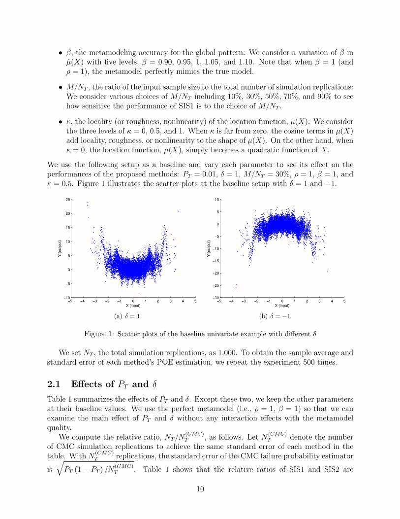
• δ, the difference between the original input density, f , and the optimal IS density,qSIS1 (or qSIS2): We want to investigate how the computational gains of SIS1 and SIS2change when the optimal IS density is more different from the original input density,f . Note that the original input density, f , is a standard normal density with a modeat 0. When δ = 1, qSIS1 and qSIS2 will focus their sampling efforts on the input regionsfar from 0, since the response variable, Y , tends to be large in such regions due tothe term, 0.95X2, in µ(X). Conversely, when δ = −1, qSIS1 and qSIS2 will focus theirsampling efforts on the regions close to 0.

• ρ, the metamodeling accuracy for the oscillating pattern: We vary ρ in µ̂(X) and σ̂(X)to control the quality of the metamodel in capturing the oscillating pattern of thetrue model with µ(X) and σ(X). We consider ρ of 0, 0.5, and 1. When ρ = 1, themetamodel mimics the oscillating pattern perfectly in both the mean and standarddeviation, whereas ρ = 0 means that the metamodel fails to capture the oscillatingpattern.

9

• β, the metamodeling accuracy for the global pattern: We consider a variation of β inµ̂(X) with five levels, β = 0.90, 0.95, 1, 1.05, and 1.10. Note that when β = 1 (andρ = 1), the metamodel perfectly mimics the true model.

• M/NT , the ratio of the input sample size to the total number of simulation replications:We consider various choices of M/NT including 10%, 30%, 50%, 70%, and 90% to seehow sensitive the performance of SIS1 is to the choice of M/NT .

• κ, the locality (or roughness, nonlinearity) of the location function, µ(X): We considerthe three levels of κ = 0, 0.5, and 1. When κ is far from zero, the cosine terms in µ(X)add locality, roughness, or nonlinearity to the shape of µ(X). On the other hand, whenκ = 0, the location function, µ(X), simply becomes a quadratic function of X.

We use the following setup as a baseline and vary each parameter to see its effect on theperformances of the proposed methods: PT = 0.01, δ = 1, M/NT = 30%, ρ = 1, β = 1, andκ = 0.5. Figure 1 illustrates the scatter plots at the baseline setup with δ = 1 and −1.

−5 −4 −3 −2 −1 0 1 2 3 4 5−10

−5

0

5

10

15

20

25

X (input)

Y (

outp

ut)

(a) δ = 1

−5 −4 −3 −2 −1 0 1 2 3 4 5−30

−25

−20

−15

−10

−5

0

5

10

X (input)

Y (

outp

ut)

(b) δ = −1

Figure 1: Scatter plots of the baseline univariate example with different δ

We set NT , the total simulation replications, as 1,000. To obtain the sample average andstandard error of each method’s POE estimation, we repeat the experiment 500 times.

2.1 Effects of PT and δ

Table 1 summarizes the effects of PT and δ. Except these two, we keep the other parametersat their baseline values. We use the perfect metamodel (i.e., ρ = 1, β = 1) so that we canexamine the main effect of PT and δ without any interaction effects with the metamodelquality.

We compute the relative ratio, NT/N(CMC)T , as follows. Let N

(CMC)T denote the number

of CMC simulation replications to achieve the same standard error of each method in thetable. With N

(CMC)T replications, the standard error of the CMC failure probability estimator

is

√PT (1− PT ) /N

(CMC)T . Table 1 shows that the relative ratios of SIS1 and SIS2 are

10

comparable to each other and clearly better than BIS, and that they generally decreaseas PT gets smaller. That is, the efficiencies of the SIS methods against CMC improve asPT gets close to zero. For example, when δ = 1 and PT are 0.10, 0.05, and 0.01, SIS1requires 51%, 32%, and 2.5% of the CMC simulation efforts to achieve the same estimationaccuracy, respectively (in other words, CMC needs about twice, three times, and forty timesmore simulation efforts than SIS1, respectively.) These remarkable computational savingsare also observed in our case study with the wind turbine simulators (see Table 5 of thepaper). Specifically, SIS1 and SIS2 respectively lead to 4.9% and 5.9% of the relative ratiosfor edgewise bending moments with l = 9,300 kNm. Note that the corresponding sampleaverages, namely 0.00992 and 0.01005, are close to the failure probability of PT = 0.01.

Table 1 also shows that the computational gains of SIS1 and SIS2 are much more signif-icant when δ = 1 (i.e., when f and qSIS1 (or qSIS2) are quite different) than when δ = −1.This finding is intuitive and also consistent with the observation in the wind turbine simu-lation that the computational gains of SIS1 and SIS2 for the edgewise bending moments aremuch more remarkable than those for the flapwise bending moments. Interestingly, whenδ = −1, BIS has no advantage over CMC, whereas the proposed methods still lead to lowerstandard errors than CMC.

Table 1: POE estimation results with different δ and PT

δ = 1 δ = −1Method PT PT

0.10 0.05 0.01 0.10 0.05 0.01

SIS1 Sample Average 0.1004 0.0502 0.0100 0.1001 0.0500 0.0100Standard Error 0.0068 0.0039 0.0005 0.0090 0.0062 0.0026Relative Ratio 51% 32% 2.5% 90% 81% 68%

SIS2 Sample Average 0.0999 0.0501 0.0100 0.1001 0.0500 0.0099Standard Error 0.0069 0.0042 0.0006 0.0086 0.0064 0.0028Relative Ratio 53% 37% 3.6% 82% 86% 79%

BIS Sample Average 0.1002 0.0505 0.0101 0.1009 0.0503 0.0101Standard Error 0.0089 0.0068 0.0014 0.0095 0.0067 0.0031Relative Ratio 88% 97% 20% 100% 95% 97%

CMC Sample Average 0.1005 0.0506 0.0100 0.1005 0.0498 0.0100Standard Error 0.0092 0.0070 0.0030 0.0096 0.0071 0.0031

2.2 Effects of metamodel accuracy

Now, we consider how computational efficiency varies when the metamodel accuracy changes.First, we study the effect of ρ, the metamodeling accuracy for the oscillating pattern. Wekeep all other parameters at their baseline values. The results in Table 2 suggest that thestandard errors for SIS1, SIS2, and BIS increase as ρ decreases (i.e., the metamodel qualitydeteriorates). However, the standard errors for both SIS1 and SIS2 increase more slowly thanfor BIS as ρ decreases. Also, SIS1 and SIS2 produce lower standard errors than BIS by 50-85% and CMC by 40-85%. Interestingly, the increase of the SIS2’s standard error is minimal,

11

indicating that SIS2 is the least sensitive to the metamodel quality. The performance of BISdiffers significantly depending on the metamodel quality, and BIS generates an even higherstandard error than CMC when ρ = 0.

Table 2: POE estimation results with different ρ

Methodρ

1.00 0.50 0

SIS1Sample Average 0.0100 0.0100 0.0101Standard Error 0.0005 0.0008 0.0017


BISSample Average 0.0101 0.0100 0.0102Standard Error 0.0014 0.0018 0.0063

CMCSample Average 0.0099 0.0099 0.0099Standard Error 0.0030 0.0030 0.0030

Second, we consider the effect of β, the metamodeling accuracy for the global pattern.We keep all other parameters at their baseline values. The results in Table 3 do not showany clear patterns to explain the impact of the metamodel accuracy of the global patternon the performances of SIS1 and SIS2. However, in all cases, SIS1 and SIS2 outperform BISand CMC, reducing the standard errors by 45-70% and 80-85%, respectively.

Table 3: POE estimation results with different β

Methodβ

0.90 0.95 1.00 1.05 1.10

SIS1Sample Average 0.0101 0.0101 0.0100 0.0101 0.0101Standard Error 0.0005 0.0005 0.0005 0.0005 0.0005

SIS2Sample Average 0.0101 0.0100 0.0100 0.0100 0.0101Standard Error 0.0006 0.0006 0.0006 0.0006 0.0006

BISSample Average 0.0101 0.0100 0.0101 0.0101 0.0101Standard Error 0.0013 0.0016 0.0014 0.0013 0.0011

CMCSample Average 0.0100 0.0100 0.0099 0.0100 0.0099Standard Error 0.0031 0.0031 0.0030 0.0030 0.0030

Third, we investigate the effect of the metamodel quality on the computational gains ofthe proposed methods as the failure probability gets smaller, when the metamodel is poor.Specifically, we consider the cases of (ρ = 0.5, β = 1), (ρ = 0, β = 0.6), and (ρ = 0, β = 1.2).We keep all other parameters at their baseline values. Table 4 shows that the computationalefficiencies of SIS1 and SIS2 are substantially better than BIS in all cases. Similar to thepattern in Table 2, SIS2 tends to perform better than SIS1 when the metamodel is inaccurate,and when PT changes from 0.10 to 0.01, the efficiencies of SIS1 and SIS2 improve remarkably.However, we note that there are some cases (e.g., SIS1 with ρ = 0, β = 1.2 and SIS2 withρ = 0, β = 0.6) where the efficiency slightly diminishes when PT changes from 0.10 to 0.05.

12

This result indicates that if the metamodel is inaccurate, the efficiencies of SIS1 and SIS2do not necessarily improve when smaller PT is estimated. Even so, SIS1 and SIS2 performmuch better than BIS.

Table 4: POE estimation results with different ρ and β

ρ = 0.5, β = 1 ρ = 0, β = 0.6 ρ = 0, β = 1.2Method PT PT PT

0.10 0.05 0.01 0.10 0.05 0.01 0.10 0.05 0.01

SIS1 Ave. 0.0998 0.0503 0.0100 0.0998 0.0503 0.0100 0.1001 0.0503 0.0102S.E. 0.0080 0.0046 0.0008 0.0104 0.0066 0.0016 0.0120 0.0090 0.0024

Ratio 71% 44% 6.4% 120% 91% 26% 160% 170% 58%SIS2 Ave. 0.0999 0.0503 0.0101 0.0999 0.0506 0.0100 0.0993 0.0503 0.0101

S.E. 0.0068 0.0045 0.0007 0.0082 0.0064 0.0009 0.0078 0.0054 0.0010Ratio 51% 42% 4.9% 75% 86% 8.1% 67% 61% 10%

BIS Ave. 0.1007 0.0502 0.0100 0.1014 0.0493 0.0105 0.1028 0.0511 0.0105S.E. 0.0134 0.0078 0.0018 0.0355 0.0086 0.0082 0.0665 0.0184 0.0104

Ratio 199% 128% 32% 1398% 155% 673% 4905% 710% 1082%CMC Ave. 0.1004 0.0506 0.0099 0.1005 0.0504 0.0100 0.1001 0.0504 0.0099

S.E. 0.0091 0.0071 0.0030 0.0093 0.0071 0.0030 0.0093 0.0070 0.0030

Notes: ‘Ave.’ denotes the sample average, ‘S.E.’ denotes the standard error, and ‘Ratio’ denotes the

relative ratio of NT /NCMCT .

2.3 Effects of the ratio, M/NT

Here, we want to see how sensitive SIS1 is to the choice of M/NT . We keep all otherparameters at their baseline values. The results in Table 5 suggest that the standard errorof the SIS1 estimator is generally insensitive to the choice of M/NT . This result is consistentwith the result of the wind turbine simulations. Note that the standard error in Table 5 ispresented up to 5 digits (not 4 digits).

Table 5: Effect of different M/NT ratios in the univariate example

M/NT Sample Average Standard Error

10% 0.0100 0.0005530% 0.0100 0.0005050% 0.0101 0.0005970% 0.0101 0.0006390% 0.0100 0.00076

13

2.4 Effects of locality, κ

We consider the effect of κ, the locality (or roughness, nonlinearity) of the location function,µ(X). We keep all other parameters at their baseline values. The results in Table 6 show thatthe standard errors for SIS1 and SIS2 slightly increase as κ increases. However, regardlessof κ, SIS1 and SIS2 outperform BIS and CMC, lowering the standard errors by 30-65% and75-90%, respectively.

Table 6: POE estimation results with different κ

Methodκ

0 0.50 1.00





2.5 Effects of variation of ε

Theoretically, SIS1 and SIS2 are reduced to deterministic importance sampling (DIS) whenthe simulator is deterministic. Recall that the standard error for DIS with qDIS is zero.Thus, in a stochastic computer model, if the uncontrollable randomness represented by ε hasa smaller level of variation, then the standard errors for SIS1 and SIS2 will get closer to zero.We conduct a numerical study to illustrate the impact of the variance of ε. We consider thesame data generating structure as before except that the variance of ε does not depend onthe input, X, but is constant:

σ2(X) = τ 2.

Equivalently, we consider Y = µ(X) + ε, where ε follows a normal distribution with meanzero and standard deviation, τ . We use the optimal IS densities for SIS1 and SIS2 with theperfect knowledge of s(X). We consider τ of 0.5, 1, 2, 4, and 8. In Figure 2, we can seethe scatter plots of Y versus X for τ of 0.5, 2, and 8, by which the variation of Y givenX is controlled. We set all other parameters at their baseline values: PT = 0.01, δ = 1,M/NT = 30%, and κ = 0.5.

Table 7 shows that as τ gets close to zero (please see from right to left), so do the standarderrors of SIS1 and SIS2. The results indicate that the proposed methods practically reduceto DIS, since the optimal DIS density makes the standard error zero for the deterministicsimulation (i.e., the case with τ = 0).

Also, Figure 3 illustrates that the optimal SIS1 and SIS2 densities are almost the sameas the BIS density when the variation of ε is very small (in the figure, we use τ = 0.5).

14

−5 −4 −3 −2 −1 0 1 2 3 4 5−40

−30

−20

−10

0

10

20

30

40

X (input)

Y (

outp

ut)

(a) τ = 0.5

−5 −4 −3 −2 −1 0 1 2 3 4 5−40

−30

−20

−10

0

10

20

30

40

X (input)

Y (

outp

ut)

(b) τ = 2

−5 −4 −3 −2 −1 0 1 2 3 4 5−40

−30

−20

−10

0

10

20

30

40

X (input)

Y (

outp

ut)

(c) τ = 8

Figure 2: Scatter plots of the baseline case with different τ

Table 7: POE estimation results with different τ = Var(ε)

Methodτ

0.50 1.00 2.00 4.00 8.00

SIS1 Sample Average 0.0102 0.0101 0.0101 0.0102 0.0100Standard Error 0.0001 0.0001 0.0005 0.0021 0.0028

SIS2 Sample Average 0.0102 0.0101 0.0101 0.0104 0.0100Standard Error 0.0001 0.0002 0.0006 0.0023 0.0028

BIS Sample Average 0.0102 0.0101 0.0100 0.0103 0.0101Standard Error 0.0002 0.0003 0.0010 0.0033 0.0033

CMC Sample Average 0.0100 0.0100 0.0099 0.0101 0.0101Standard Error 0.0030 0.0031 0.0030 0.0032 0.0031

Notes: SIS1’s standard errors for τ = 0.50 and τ = 1.00 are 0.00007 and 0.00013, respectively, in one more

digit.

Since the BIS density theoretically reduces to the DIS density for deterministic simulationand closely mimics the DIS density when τ is negligibly small, we can see that the proposedmethods practically reduce to DIS when the variation of the uncontrollable randomness isvery small.

2.6 Precision of numerical integration

When we use the numerical integration to compute the normalizing constant of an IS density,we make sure that the numerical precision is accurate enough so that the POE estimationaccuracy is unaffected. We present POE estimation results up to 5 digits after the decimalpoint. Given that we bound the numerical error by -7 orders of magnitude or smaller, thenumerical integration does not contribute to the error of POE estimation. To check theprecision, we also conduct numerical studies with the same data generating structure usedin Section 2.5. In Table 8, the sample averages and standard errors are based on 500 POEestimates. The POEs in the last column are estimated by CMC with 100 million replications.We note that the estimated POE values from SIS1 and SIS2 are the same as the values fromCMC.

15

−5 0 50

0.5

1

1.5

2

2.5

x

Den

sity

OriginalSIS1SIS2BIS

Figure 3: Density plots for SIS1, SIS2, and BIS optimal densities when τ = 0.50 along withthe original input density

3 Multivariate Example

We also design a multivariate stochastic example. We take an example in Huang et al.[4], which adds a normal stochastic noise to a deterministic example originally in Ackley[1]. We slightly revise the example in Huang et al. [4] by adding more complexity to thestochastic elements, and use the following data generating structure where the input vector,X = (X1, X2, X3), follows a multivariate normal distribution:

X ∼MVN(0, I3) ,

Y |X ∼ N(µ(X) , σ2(X)

),


µ(X) = 20δ

(1− exp

(−0.2

√1

3‖X‖2

))+ δ

(exp (1)− exp

(1

3

3∑i=1

cos(2πκXi)

)),

σ(X) = 1 + 0.7

√1

3‖X‖2 + 0.4

(1

3

3∑i=1

cos(3πXi)

),

respectively. The output, Y , with the above µ(X) and σ(X) presents a very complicatedpattern over the input domain. The metamodel for the conditional distribution, Y |X, is

16

Table 8: POE estimation results for SIS1 and SIS2, compared to the POE estimated byCMC with 100 million replications, for different τ = Var(ε)

Sample Averageτ (Standard Error) CMC

SIS1 SIS2

0.500.0102 0.0102 0.0102

(0.0001) (0.0001)

1.000.0101 0.0101 0.0101

(0.0001) (0.0002)

2.000.0101 0.0101 0.0101

(0.0005) (0.0006)

N(µ̂(X) , σ̂2(X)), where

µ̂(X) = 20βδ

(1− exp

(−0.2

√1

3‖X‖2

))+ ρδ

(exp (1)− exp

(1

3

3∑i=1

cos(2πκXi)

)),

σ̂(X) = 1 + 0.7

√1

3‖X‖2 + 0.4ρ

(1

3

3∑i=1

cos(3πXi)

).

The parameters in the above equations take similar roles in the univariate example. Weuse the same baseline setup we used in the univariate example, namely, PT = 0.01, δ = 1,M/NT = 30%, ρ = 1, β = 1, and κ = 0.5. We explain each parameter as follows.

• PT , the magnitude of target failure probability: Based on 10 million CMC simu-lation replications, we decide l that corresponds to the target failure probability,PT = P (Y > l). We consider the three levels of PT , 0.10, 0.05, and 0.01.

• δ, the difference between the original input density, f , and the optimal IS density,qSIS1(or qSIS2): We consider δ of 1 or−1. The densities, f and qSIS1 (or qSIS2), are moredifferent from each other when δ = 1 than when δ = −1. Note that the original inputdensity, f , has the highest likelihood at the origin. When δ = 1, qSIS1 and qSIS2 will fo-cus their sampling efforts on the regions far from the origin, since the response variable,

Y , tends to be large in such regions due to the term, 20(

1− exp(−0.2

√13‖X‖2

)), in

µ(X). Conversely, when δ = −1, qSIS1 and qSIS2 will focus their sampling efforts onthe regions close to the origin.

• ρ, the metamodeling accuracy for the oscillating pattern: We consider ρ of 0, 0.5, and1. When ρ = 1, the metamodel mimics the oscillating pattern perfectly, whereas ρ = 0implies that the metamodel captures no oscillating term.

• β, the metamodeling accuracy for the global pattern: We consider β = 0.95, 1, and1.05. Note that when β = 1 (and ρ = 1), the metamodel perfectly mimics the truemodel.

17

• M/NT , the ratio of the input sample size to the total number of simulation replications:We consider M/NT of 10%, 30%, 50%, 70%, and 90%.

• κ, the locality (or roughness, nonlinearity) of the location function, µ(X): We considerthe four levels of κ, 0, 0.5, 1, and 2. When κ is far from zero, the cosine terms in µ(X)add locality, roughness, or nonlinearity to the shape of µ(X). On the other hand,when κ = 0, the location function, µ(X), simply becomes a monotonically increasingfunction of ‖X‖.

3.1 Effects of PT and δ

Table 9 summarizes the effects of PT and δ. We keep all other parameters at their baselinevalues. Similar to the univariate example, the experiment results suggest that the compu-tational gains of SIS1 and SIS2 against CMC increase as PT gets smaller. We also see thatthe computational gains of SIS1 and SIS2 are more significant when δ = 1 (i.e., f and qSIS1(or qSIS2) are quite different) than when δ = −1. In all cases, SIS1 and SIS2 perform betterthan BIS and CMC.

We note that when δ = 1, the relative ratios of SIS1 and SIS2 decrease more slowly thanthe univariate input example results in Table 1. Specifically, for PT = 0.01, SIS1 and SIS2yield 2.5% and 3.6% of the relative ratios in Table 1; but, both methods give 29% of therelative ratio in Table 9. We attribute such differences in the two example results to thedifferences in the data generating structures. The data generating structure of the univariateexample in Section 2 and the multivariate example in Section 3 are different not only in theinput dimension but also in the mean function, µ(x), and the standard deviation function,σ(X). We detail this point in Section 3.5.

Table 9: POE estimation results with different δ and PT for the multivariate example

δ = 1 δ = −1Method PT PT

0.10 0.05 0.01 0.10 0.05 0.01

SIS1 Sample Average 0.1002 0.0501 0.0100 0.1000 0.0500 0.0100Standard Error 0.0070 0.0046 0.0017 0.0072 0.0051 0.0020Relative Ratio 54% 45% 29% 58% 55% 40%




18

3.2 Effects of metamodel accuracy

We consider the effect of ρ, the metamodeling accuracy for the oscillating pattern. We keepall other parameters at their baseline values. Similar to the univariate example, Table 10shows that the standard errors of the SIS1 and SIS2 estimators increase as ρ decreases. Also,the standard error for SIS2 increases more slowly than that for SIS1, which shows that SIS2is less sensitive than SIS1 to the metamodel quality. It appears that the performance of BISis the most sensitive to the metamodel quality. In all cases, SIS1 and SIS2 lead to smallerstandard errors than BIS and CMC by 20–60% and 20–50%, respectively.

Table 10: POE estimation results with different ρ in the multivariate example

Methodρ

1.00 0.50 0





Notes. At ρ = 1, standard errors for SIS1 and SIS2 are 0.00167 and 0.00163, respectively, in one more digit.

We consider the effect of β, the metamodeling accuracy for the global pattern. We keepall other parameters at their baseline values. Table 11 shows that the standard errors of theSIS1 and SIS2 estimators do not vary significantly, so the performances of SIS1 and SIS2are insensitive to the metamodeling accuracy for the global pattern in this example. In allcases, SIS1 and SIS2 outperform BIS and CMC, providing lower standard errors than BISand CMC by 25–40% and 45-50%, respectively. .

Table 11: POE estimation results with different β in the multivariate example

Methodβ

0.95 1.00 1.05





19

3.3 Effects of the ratio, M/NT

We want to see how sensitive SIS1 is to the choice of M/NT . We keep all other parametersat their baseline values. The results in Table 12 suggest that the standard error of the SIS1estimator is generally insensitive to the choice of M/NT as we observed in the univariateexample and the wind turbine simulations. Note that the standard error is presented up to5 digits (not 4 digits).

Table 12: Effect of different M/NT ratios in the multivariate example

M/NT Sample Average Standard Error

10% 0.0100 0.0016830% 0.0100 0.0016750% 0.0100 0.0016870% 0.0100 0.0017390% 0.0100 0.00185

3.4 Effects of locality, κ

We consider the effect of κ, the locality (or roughness, nonlinearity) of the location function,µ(X). We keep all other parameters at their baseline values. The results in Table 13 suggestthat κ has little effect on the standard errors of the SIS1 and SIS2 estimators in this specificexample. For all κ values, SIS1 and SIS2 lead to smaller standard errors than BIS and CMCby 20–50% and 45–50%, respectively.

Table 13: POE estimation results with different κ in the multivariate example

Methodκ

0 0.5 1 2

SIS1Sample Average 0.0099 0.0100 0.0101 0.0099Standard Error 0.0017 0.0017 0.0016 0.0016

SIS2Sample Average 0.0101 0.0100 0.0100 0.0100Standard Error 0.0017 0.0017 0.0016 0.0016

BISSample Average 0.0101 0.0100 0.0101 0.0100Standard Error 0.0031 0.0022 0.0033 0.0031

CMCSample Average 0.0102 0.0101 0.0102 0.0103Standard Error 0.0031 0.0031 0.0031 0.0032

3.5 Analysis with the univariate input

In Section 3.1, as PT gets smaller, we observe that the relative ratio of SIS1 and SIS2 withδ = 1 decreases more slowly than those in the univariate example (see Tables 1 and 9 withδ = 1). These different patterns in the two numerical examples are mainly due to thedifferent data generating structure not only in the input dimension but also in the mean

20

function, µ(x), and the standard deviation function, σ(X). For the univariate example inSection 2, we take a deterministic simulation example in Cannamela et al. [2] and modify itby adding stochastic elements to it, whereas for the multivariate example in Section 3, weadd a normal stochastic noise to a deterministic multivariate example originally in Ackley[1]. In the sequel, we call these univariate and multivariate examples as Cannamela1D andAckley3D, respectively, based on their respective sources [1, 2].

To clarify the different patterns in Cannamela1D and Ackley3D, we devise a new univariateexample which is one-dimensional version of Ackley3D, and we call this new example asAckley1D. Specifically, we consider the following data generating structure:

X ∼ N(0, 1) ,

Y |X ∼ N(µ(X) , σ2(X)

),


µ(X) = 20δ (1− exp (−0.2|X|)) + δ (exp (1)− exp (cos(2πκX))) ,

σ(X) = 1 + 0.7|X|+ 0.4 (cos(3πX)) ,

respectively.The metamodel for the conditional distribution, Y |X, is N(µ̂(X) , σ̂2(X)), where

µ̂(X) = 20βδ (1− exp (−0.2|X|)) + ρδ (exp (1)− exp (cos(2πκX))) ,

σ̂(X) = 1 + 0.7|X|+ 0.4ρ (cos(3πX)) .

For the experiments of Ackley1D, we use the same baseline setup used in Cannamela1D andAckley3D, namely, PT = 0.01, δ = 1, M/NT = 30%, ρ = 1, β = 1, and κ = 0.5. Notethat ρ = 1, β = 1 imply that the metamodel is perfect so that the optimal IS densities andallocations can be used.

Table 14 below compares the results of Ackley1D and Ackley3D. We note that the relativeratios of SIS1 and SIS2 for Ackley1D, namely, 15% and 17%, are smaller than those ofAckley3D, namely, 29% and 29%. Yet, the performances for Ackley1D are not as remarkableas those for Cannamela1D in Table 1, namely, 2.5% and 3.6%. Such performance differencesin Cannamela1D and Ackley1D can be explained mainly by the difference in their underlyingdata generating structures: See Figure 4 below, where we plot the optimal SIS1 density alongwith the original input density for both examples. Apparently, the optimal SIS1 density forCannamela1D is deviating much more from the original input density than that for Ackley1Dis. We observe the similar pattern for SIS2. This explains the better performances of SIS1and SIS2 for Cannamela1D.

Obviously, the computational gain of SIS1 and SIS2 over CMC largely depends on thegeneral trend represented by the location parameter functions, µ(X). In addition, the scaleparameter functions, σ(X), also make a difference in the performance of SIS1 and SIS2 forCannamela1D and Ackley1D. We plot 20,000 input-output pairs, (X, Y )’s, generated fromthe baseline setups for Cannamela1D and Ackley1D in Figures 5(a) and (b), respectively. Wedraw the solid horizontal line in each plot to indicate the resistance level, l, correspondingto PT = 0.01. We observe that the location parameter functions, µ(X), in both examples

21

tend to have large values at the regions where f(X) is small. However, the scale parameterfunctions, σ(X), lead to a major difference around the region, (−2,−1)∪ (1, 2), where µ(X)itself is not yet close to l but many responses of Ackley1D in Figure 5(b) exceed l unlikeCannamela1D in Figure 5(a). Accordingly, we observe the relevant peaks at (−2,−1)∪ (1, 2)in Figure 4(b), which disperse sampling efforts in a larger input area and make qSIS1 (andqSIS2) more overlapped with f for Ackley1D.

Table 14: POE estimation results with different input dimension and target failure proba-bility, PT , for the numerical examples based on Ackley [1]

Ackley1D Ackley3DMethod PT PT

0.10 0.05 0.01 0.10 0.05 0.01





−5 −4 −3 −2 −1 0 1 2 3 4 50

0.2

0.4

0.6

0.8

1

1.2

1.4

1.6

1.8

2

x

De

nsity

Original

SIS1

(a) Cannamela1D

−5 −4 −3 −2 −1 0 1 2 3 4 50

0.2

0.4

0.6

0.8

1

1.2

1.4

1.6

1.8

2

x

De

nsity

Original

SIS1

(b) Ackley1D

Figure 4: Comparison of the optimal SIS1 density and the original input density for the twoexamples

In summary, the performance of the proposed methods will depend on the characteristicsof the simulation model. Note that the variances of the proposed estimators depend only on

22

−5 −4 −3 −2 −1 0 1 2 3 4 5−10

−5

0

5

10

15

20

25

X (input)

Y (

outp

ut)

(a) Cannamela1D

−5 −4 −3 −2 −1 0 1 2 3 4 5−10

−5

0

5

10

15

20

25

X (input)

Y (

outp

ut)

(b) Ackley1D

Figure 5: Scatter plots of the data generated from the baseline data generating structures: thesolid horizontal line is the quantile, l, corresponding to PT = 0.01

the functions, s(x) and f(x), according to Theorems 1 and 2 (note that the SIS1 and SIS2densities are also expressed in s(x) and f(x)) and both functions are determined by the truedata generating structure. Lastly, we remark that the higher relative ratios of SIS1 and SIS2for Ackley3D compared to those for Ackley1D should not be generalized as that the inputdimension negatively affects the performance of SIS1 and SIS2. In the case of Ackley3D, dueto the highly oscillating response over the three dimensional input space, the sampling effortsare more distributed in the larger input space and the resulting qSIS1 (and qSIS2) is moreoverlapped with f , compared to the case of Ackley1D. However, even with high dimensionalinput vectors, significant computational reduction can be achieved when the joint density ofthe input vector, f , and the optimal SIS1 (and SIS2) density, qSIS1 (and qSIS2), are different.

3.6 Summary

Overall, we observe similar patterns both in the univariate example and the multivariateexample. These patterns are also consistent with the wind turbine simulation results. Fora wide range of parameter settings, the performances of SIS1 and SIS2 are superior to BISand CMC.

4 Implementation Details with Wind Turbine Simula-

tors

In this section, we present the implementation details with wind turbine simulators.

23

4.1 NREL simulators and the original input distribution

The NREL simulators used in this study include TurbSim [6] and FAST [7]. Given awind condition (e.g., 10-minute average wind speed), TurbSim produces a three-dimensionalstochastic wind profile. FAST, taking the generated wind profile as an input, simulates loadresponses (or loads) at turbine subsystems such as blades and shafts. Noting that there aremany types of load responses, we limit our study to consider edgewise and flapwise bendingmoments at a blade root as output variables, where edgewise (flapwise) bending momentsimply structural loads parallel (perpendicular) to the rotor span at a blade root. These twoload types are of great concern in ensuring a wind turbine’s structural reliability [10].

As in [10], we use the same turbine specification for an onshore version of an NREL5-MW baseline wind turbine [8]. The target turbine operates within a specified wind speedrange between the cut-in speed, xin = 3 meter per second (m/s), and the cut-out speed,xout = 25 m/s. Following wind industry practice and the international standard, IEC 61400-1 [5], we use a 10-minute average wind speed as an input, X, to the simulators. We use aRayleigh density for X with a truncated support of [xin, xout] as in [10]:

f(x) =fR(x)

FR(xout)− FR(xin),

where FR (x) = 1− e−x2/2τ2 denotes the cumulative distribution function of Rayleigh distri-bution with a scale parameter, τ =

√2/π · 10 (unit: m/s). Also, fR denotes the Rayleigh

density function with the same scale parameter.

4.2 Acceptance rates of the acceptance-rejection algorithm

We use the acceptance-rejection algorithm in the implementation. The algorithm’s accep-tance rate is equal to the normalizing constant of each IS density because we use the originalinput density, f , as an instrumental (or auxiliary) density for the algorithm [9]. Note thatthe normalizing constants are Cq1 for SIS1, Cq2 for SIS2, and P (Y > l) for BIS.

The acceptance rates differ, depending on POE, P (Y > l). In our implementation, whenPOE is around 0.05 (i.e., edgewise moments with l = 8,600 kNm or flapwise moments withl = 13,800 kNm), the acceptance rates are 5–21%. When POE is around 0.01 (i.e., edgewisemoments with l = 9,300 kNm or flapwise moments with l = 14,300 kNm), the acceptancerates are 1–14%. In practice, the computational cost of the acceptance-rejection algorithmwould be insignificant. For example, sampling thousands of inputs from the IS densities is amatter of seconds, whereas thousands of the NREL simulation replications can take days.

4.3 Goodness-of-fit test for the model

In constructing the metamodel, we assume no prior information on important area, so sam-pling X from the uniform distribution would be generally suitable. We use the GEV distribu-tion for approximating the conditional POE given X regardless of the choice of distributionfor X, and the GEV distribution is employed over the entire input space with varying loca-tion and scale parameters, µ(X) and σ(X). In our implementation, we use the metamodelbased on the GEV distribution to approximate the theoretically optimal IS density, qSIS1 (or

24

qSIS2). That is, the GEV distribution is used as a means to find the good IS density. Then,we run the real simulators (not the metamodel) to gather Y for each X sampled from qSIS1(or qSIS2).

Obviously, the metamodel quality affects the performance of the proposed approach.Therefore, in our study, we used the GEV goodness-of-fit to check if the GEV provides agood approximation of the conditional distribution over the entire input space as shown inthe paper. In this section, we additionally check if the GEV is suitable in the area whereX is likely sampled. Noting that high edgewise (flapwise) bending loads are most likelyobserved when wind speeds are between 17 and 25 (11 and 19), we take 50 observations eachat 17, 19, · · · , 25 (11, 13, · · · , 19) m/s and conduct Kolmogorov-Smirnov (KS) tests to assessthe goodness-of-fit of the GEV distribution at each wind speed. The results in Table 15below support the use of GEV distribution for edgewise and flapwise bending moments, asthe p-values are greater than a reasonable significance level, say, 5%.

Table 15: KS tests for GEV at imporant wind speeds

Edgewise bending moments Flapwise bending momentsx (m/s) p-value x (m/s) p-value

17 0.34 11 0.3119 0.60 13 0.5221 0.89 15 0.3523 0.19 17 0.5725 0.64 19 0.36

4.4 CMC simulations

We want to ensure that the estimations of N(CMC)T are accurate, which are used to compute

the relative ratios in Tables 5 and 6 of the paper. Thus, we run CMC simulations withN

(CMC)T corresponding to SIS1 and SIS2 for the flapwise moment with l = 13, 800 kNm and

compute the standard errors based on 50 repetitions. The correspondingN(CMC)T for SIS1 and

SIS2 are 6,219 and 4,762, respectively. In addition, we run simulations with N(CMC)T = 5, 000

and N(CMC)T = 6, 000. With N

(CMC)T of 6,000 and 6,219, we obtain the CMC’s standard

error of 0.0028, which is the same with the SIS1’s standard error with NT = 2, 000. WithN

(CMC)T = 4, 762 and N

(CMC)T = 5, 000, we obtain the CMC’s standard errors of 0.0036 and

0.0033, respectively, which are close to the SIS2’s standard error of 0.0032. We omit theCMC implementation for other cases due to the intensive computational requirement.

References

[1] Ackley, D. H. (1987). A connectionist machine for genetic hillclimbing. Boston: KluwerAcademic Publishers.

[2] Cannamela, C., Garnier, J., and Iooss, B. (2008). Controlled stratification for quantileestimation. The Annals of Applied Statistics, 2(4):1554–1580.

25

[3] Courant, R. and Hilbert, D. (1989). Methods of Mathematical Physics. New York: Wiley.[4] Huang, D., Allen, T. T., Notz, W. I., and Zeng, N. (2006). Global optimization of stochas-

tic black-box systems via sequential kriging meta-models. Journal of global optimization,34(3):441–466.

[5] International Electrotechnical Commission (2005). IEC/TC88, 61400-1 ed. 3, Wind Tur-bines - Part 1: Design Requirements.

[6] Jonkman, B. J. (2009). TurbSim user’s guide: version 1.50. Technical Report NREL/TP-500-46198, National Renewable Energy Laboratory, Golden, Colorado.

[7] Jonkman, J. M. and Buhl Jr., M. L. (2005). FAST User’s Guide. Technical ReportNREL/EL-500-38230, National Renewable Energy Laboratory, Golden, Colorado.

[8] Jonkman, J. M., Butterfield, S., Musial, W., and Scott, G. (2009). Definition of a 5-MWreference wind turbine for offshore system development. Technical Report NREL/TP-500-38060, National Renewable Energy Laboratory, Golden, Colorado.

[9] Kroese, D. P., Taimre, T., and Botev, Z. I. (2011). Handbook of Monte Carlo Methods.New York: John Wiley and Sons.

[10] Moriarty, P. (2008). Database for validation of design load extrapolation techniques.Wind Energy, 11(6):559–576.

26

tch-13-190: supplements

Documents