tcmullet_dissertation_final
TRANSCRIPT


EFFECTS OF SNOWMOBILE NOISE AND ACTIVITY
ON A BOREAL ECOSYSTEM IN SOUTHCENTRAL ALASKA
A
DISSERTATION
Presented to the Faculty
of the University of Alaska Fairbanks
in Partial Fulfillment of the Requirements
for the Degree of
DOCTOR OF PHILOSOPHY
By
Timothy Carl Mullet, M.S.
Fairbanks, AK
December 2014
v
Abstract
Snowmobiling is a popular winter activity in northern regions of North America.
Although snowmobiles are important utility vehicles and serve as a means of outdoor recreation,
their activity is known to affect plants and animals. These effects have been a growing concern
over the past 20 years as a result of increased snowmobile activity into once inaccessible natural
areas. Minimizing the impacts of snowmobiles on biota, preserving the quality and character of
wilderness areas, and providing adequate access to snowmobilers for traditional activities has
been a challenge for public land managers in Alaska. To address the effects that snowmobiles
have on ecological systems at site-specific and landscape-level scales, I conducted a study in the
Kenai National Wildlife Refuge, a boreal ecosystem located in southcentral Alaska, to determine
1) the response of woody wetland plants to snowmobile traverses at varying snow depths, 2) the
temporal and spatial variation of a winter soundscape with emphasis on anthrophony, in general,
and snowmobile noise, specifically, 3) the effects of snowmobile noise on wilderness character
and naturalness, and 4) the spatial and physiological response of moose (Alces alces) to
snowmobile activity and noise. I used a combination of traditional experimental designs and
statistics, machine learning, and spatially-explicit predictive modeling to assess the effects
snowmobile activity has on these four issues. I found that snowmobile activity reduced the
number of living stems and inhibited the growth of woody wetland plants by direct contact with
protruding vegetation above the snow and indirectly from snow compaction. Snowmobile noise
was not a large contributor of noise to the soundscape but was pervasive in remote areas.
Snowmobile noise affected a significant area of Congressionally-designated wilderness altering
the naturalness and character of the wilderness soundscape. Moose exhibited a distinct spatial
partitioning and avoidance from snowmobile activity and developed areas (i.e., oil and gas

vi
compressors) at the landscape-level but at a site-specific scale snowmobile traffic and noise had
no apparent affect on the stress hormone levels of moose that were selecting habitats close to
snowmobile trails. I detected these impacts at both site-specific locations and across large spatial
scales indicating that snowmobile effects are more than just localized disturbances. Based on
these findings, I conclude that snowmobile noise and activity is an additional and unnatural
forcing function on a boreal ecosystem already stressed by the harsh environmental conditions of
winter.

vii
This dissertation is dedicated to the three most important people in my life:
Monica, Thera, and Emma

ix
Table of Contents
Page
Signature Page ................................................................................................................................. i
Title Page ....................................................................................................................................... iii
Abstract ............................................................................................................................................v
Dedication Page ............................................................................................................................ vii
Table of Contents ........................................................................................................................... ix
List of Figures ................................................................................................................................xv
List of Tables ............................................................................................................................... xxi
List of Appendices .......................................................................................................................xxv
Acknowledgements ................................................................................................................... xxvii
Chapter 1 An Introduction to the Ecological Effects of Snowmobiles ............................................1
1.1 Why Study the Ecological Effects of Snowmobiles? ..........................................1
1.2 A Systems Approach to Understanding the Ecological Effects of
Snowmobiles .......................................................................................................3
1.3 Snowmobile Effects on Environmentally-Stressed State Variables ....................6
1.3.1 Snow and Vegetation ..........................................................................6
1.3.2 Wildlife ...............................................................................................8
1.3.2.1 Small Mammals .............................................................10
1.3.2.2 Ungulates .......................................................................11
1.3.2.2.1 White-tailed Deer ....................................11
1.3.2.2.2 Caribou....................................................12
1.3.2.2.3 Moose......................................................13

x
1.3.2.2.4 Elk and Bison ..........................................14
1.3.2.3 Coyotes ..........................................................................14
1.4 Snowmobile Effects on Specific Aspects of Wildlife Physiology ....................15
1.5 Soundscape Ecology, Wilderness, and Snowmobile Noise Effects on
Wildlife ..............................................................................................................17
1.5.1 Soundscape Ecology ...........................................................................17
1.5.2 Congressionally-Designated Wilderness and Sound ..........................19
1.5.3 Snowmobile Noise and its Effects on Wildlife ..................................22
1.6 Summary ...........................................................................................................24
1.7 Objectives ..........................................................................................................25
1.8 Study Area .........................................................................................................28
1.9 Organization of Dissertation .............................................................................29
Chapter 2 Effects of Snowmobile Traffic on Three Species of Wetland Shrubs in Southcentral
Alaska ..........................................................................................................................31
2.1 Abstract .............................................................................................................31
2.2 Introduction .......................................................................................................32
2.3 Methods .............................................................................................................37
2.3.1 Hypotheses .........................................................................................37
2.3.2 Sampling Design ................................................................................38
2.3.3 Statistical Analysis .............................................................................40
2.4 Results ...............................................................................................................41
2.4.1 Snow Compaction ..............................................................................41
2.4.2 Vegetation Response at Snow Depths ≥50 cm ...................................41

xi
2.4.3 Vegetation Response at Snow Depths <50 cm ..................................47
2.4.4 Comparison between Treatment Groups ............................................48
2.5 Discussion .........................................................................................................48
Chapter 3 Temporal and Spatial Variation of a Winter Soundscape in Alaska .............................51
3.1 Abstract .............................................................................................................51
3.2 Introduction .......................................................................................................52
3.3 Methods and Materials ......................................................................................55
3.3.1 Sample Design ....................................................................................55
3.3.1.1 Spatial Sampling .............................................................55
3.3.1.2 Sound Sampling and Data Acquisition ...........................56
3.3.1.3 Discriminating Soundscape Components .......................59
3.3.2 Soundscape Analysis ..........................................................................63
3.3.3 Building Spatially Explicit Predictive Models and Mapping
Soundscape Components....................................................................64
3.4 Results ...............................................................................................................67
3.4.1 Composition of Soundscape Components..........................................67
3.4.2 Soundscape Power by Frequency .......................................................69
3.4.3 Temporal Variation of Soundscape Components...............................73
3.4.4 Spatial Variation of Soundscape Components ...................................81
3.4.4.1 Biophony .........................................................................81
3.4.4.2 Anthrophony ...................................................................86
3.4.4.3 Geophony ........................................................................90
3.4.4.4 Silence .............................................................................94

xii
3.5 Discussion .........................................................................................................97
Chapter 4 Snowmobile Noise Effects on Naturalness and Wilderness Character in the Kenai
National Wildlife Refuge, Alaska ..............................................................................105
4.1 Abstract ...........................................................................................................105
4.2 Introduction .....................................................................................................107
4.3 Methods and Materials ....................................................................................115
4.3.1 Sound Sampling and Sound Data Acquisition .................................115
4.3.2 Modeling Snowmobile Noise and Natural Quiet .............................116
4.3.3 Quantifying the Area of Snowmobile Noise and Natural Quiet in
Wilderness ........................................................................................118
4.4 Results .............................................................................................................118
4.4.1 Proportion of Snowmobile Noise and Natural Quiet in Wilderness
and Non-wilderness Areas ...............................................................118
4.4.2 Model Predictions and Spatial Distribution of Snowmobile Noise
and Natural Quiet .............................................................................120
4.4.2.1 Snowmobile Noise Model and Affected Area of
Wilderness ....................................................................120
4.4.2.2 Natural Quiet Model and Areas of Quiet Wilderness
Hotspots ........................................................................125
4.5 Discussion .......................................................................................................127
Chapter 5 Spatial and Physiological Responses of Moose to Snowmobile Activity and
Noise ............................................................................................................................135
5.1 Abstract ...........................................................................................................135

xiii
5.2 Introduction .....................................................................................................137
5.3 Methods and Materials ....................................................................................144
5.3.1 Determining the Spatial Response of Moose to
Snowmobile Activity ........................................................................144
5.3.1.1 Aerial Surveys and Quantifying Moose and Snowmobile
Activity .........................................................................144
5.3.1.2 Building Spatially Explicit Models of Moose and
Snowmobile Activity ....................................................145
5.3.1.3 Spatial Comparison of Predicted Moose and Snowmobile
Activity .........................................................................146
5.3.2 Determining the Physiological Response of Moose to Snowmobile
Activity and Noise ............................................................................146
5.3.2.1 Sampling Moose Pellets for Immunoassay and Hormone
Analysis.........................................................................146
5.3.2.2 Monitoring Snowmobile Traffic ...................................149
5.3.2.3 Sound Sampling, Sound Data Acquisition, and Modeling
Snowmobile Noise ........................................................149
5.3.2.4 Data Analysis of Stress, Snowmobile Traffic,
and Noise ......................................................................149
5.4 Results .............................................................................................................153
5.4.1 Spatial Response of Moose to Snowmobile Activity .......................153
5.4.2 Moose Physiological Response to Snowmobile Traffic ...................162
5.4.3 Moose Physiological Response to Snowmobile Noise ....................162
xiv
5.5 Discussion .......................................................................................................171
Chapter 6 Assessment of the Ecological Effects of Snowmobiles ..............................................181
6.1 Conclusions .....................................................................................................181
6.2 Management Recommendations .....................................................................186
Literature Cited ............................................................................................................................191
Appendices ...................................................................................................................................217

xv
List of Figures
Page
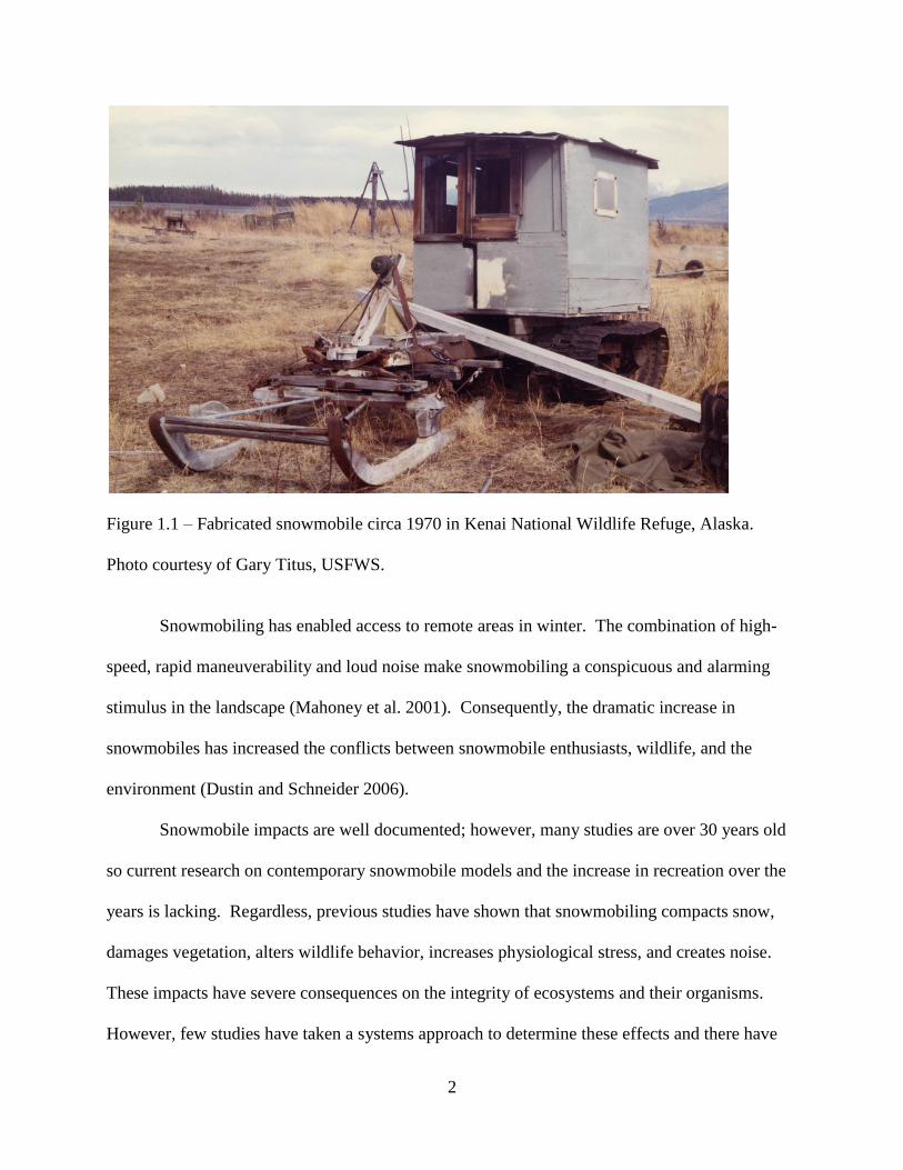
Figure 1.1: Fabricated snowmobile circa 1970 in Kenai National Wildlife Refuge, Alaska.
Photo courtesy of Gary Titus, USFWS .......................................................................2
Figure 1.2: Framework of a snowmobile-affected system. Key state variables such as plants,
wildlife, soundscape, and wilderness character are all components of an ecological
system susceptible to the effects of snowmobile activity .........................................28
Figure 1.3: Geographical orientation and associated landcover classes of the Kenai National
Wildlife Refuge, Alaska based on 2002 Landsat7 ETM+, USGS DEM, and ground
location data (KENWR Geodatabase) ......................................................................30
Figure 2.1: Graphical results of an a priori power analysis of 100 simulations of woody plant
stem declines following snowmobile traverses .........................................................39
Figure 2.2: Mean plant height and 95% confidence intervals from three woody shrub species
(dwarf birch, shrubby cinquefoil, and sweet gale) in comparison between control
and treatment plots (Transect 2 is ≥50 cm snow depth; Transect 3 is <50 cm snow
depth) before (Pretreatment) and after (Post-treatment) 10 snowmobile
traverses ....................................................................................................................43
Figure 2.3: Mean number of living stems and 95% confidence intervals from three woody
shrub species (dwarf birch, shrubby cinquefoil, and sweet gale) in comparison
between control and treatment plots (Transect 2 is ≥50 cm snow depth; Transect 3
is <50 cm snow depth) before (Pretreatment) and after (Post-treatment) 10
snowmobile traverses ................................................................................................45

xvi
Figure 2.4: Mean number of dead stems and 95% confidence intervals from three woody shrub
species (dwarf birch, shrubby cinquefoil, and sweet gale) in comparison between
control and treatment plots (Transect 2 is ≥50 cm snow depth; Transect 3 is <50 cm
snow depth) before (Pretreatment) and after (Post-treatment) 10 snowmobile
traverses ....................................................................................................................47
Figure 3.1: Spatial distribution of sound recording stations in relation to a grid partition
separating the Kenai National Wildlife Refuge study area into six sample
areas ..........................................................................................................................57
Figure 3.2: Example of a spectrogram generated in the Remote Environmental Assessment
Laboratory digital sound library of a recording of light wind (wash of light blue in
the 1 kHz band width at 0-30 secs), a boreal chickadee chirping (intermittent light
blue points in the 2-3 kHz band widths at 5-20 secs), and a red squirrel chattering
(light blue series of lines between the 1-6 kHz band widths at 35-45 secs). Yellow
lines indicate separations into 1 kHz frequency band widths with their associated
normalized power spectral density values (watts/kHz) calculated from Welch
(1967) algorithm .......................................................................................................59
Figure 3.3: Proportion of sound recordings of soundscape components.....................................68
Figure 3.4: Proportion of sound recordings of anthrophonic and biophonic sound sources .......69
Figure 3.5: Mean soundscape power (watts/kHz) and 95% confidence intervals of biophony for
10 frequency intervals ...............................................................................................70
Figure 3.6: Mean soundscape power (watts/kHz) and 95% confidence intervals of anthrophony
for 10 frequency intervals .........................................................................................71
xvii
Figure 3.7: Mean soundscape power (watts/kHz) and 95% confidence intervals of geophony for
10 frequency intervals. ..............................................................................................72
Figure 3.8: Mean soundscape power (watts/kHz) and 95% confidence intervals of silence for 10
frequency intervals ....................................................................................................73
Figure 3.9: Temporal pattern of mean soundscape power and 95% confidence intervals for the
six lowest frequency intervals of biophony over a 24 hr period ...............................74
Figure 3.10: Temporal pattern of mean soundscape power and 95% confidence intervals at the
1-2 kHz interval of anthrophony over a 24 hr period ...............................................75
Figure 3.11: Temporal pattern of mean soundscape power and 95% confidence intervals at the
1-2 kHz interval of geophony over a 24 hr period. ...................................................76
Figure 3.12: Temporal pattern of mean total soundscape power and 95% confidence intervals for
all frequency intervals of silence over a 24 hr period. ..............................................77
Figure 3.13: Temporal pattern of mean total and 95% confidence intervals of soundscape power
for all frequency intervals of biophony over monthly time intervals. Letters indicate
significant differences (p < 0.05) ..............................................................................78
Figure 3.14: Temporal pattern of mean soundscape power for the 1-2 kHz frequency interval and
95% confidence intervals of anthrophony over monthly time intervals. Letters
indicate significant differences (p < 0.05) ................................................................79
Figure 3.15: Temporal pattern of mean soundscape power for the 1-2 kHz frequency interval and
95% confidence intervals of geophony over monthly time intervals. Letters indicate
significant differences (p < 0.05) ..............................................................................80

xviii
Figure 3.16: Temporal pattern of mean total soundscape power for all frequency intervals and
95% confidence intervals of silence over monthly time intervals. Letters indicate
significant differences (p < 0.05) ..............................................................................81
Figure 3.17: One predictor dependence for the top three environmental variables predicting
biophony: a) distance to urban areas, b) distance to deciduous forest, and c) distance
to rivers .....................................................................................................................83
Figure 3.18: Predicted spatial distributions of biophony in the Kenai National Wildlife Refuge
over winter 2011-2012 ..............................................................................................85
Figure 3.19: One predictor dependence for the top three environmental variables predicting
anthrophony: a) distance to urban areas, b) distance to rivers, and c) distance
to lakes ......................................................................................................................88
Figure 3.20: Predicted spatial distributions of anthrophony in the Kenai National Wildlife Refuge
over winter 2011-2012 ..............................................................................................89
Figure 3.21: One predictor dependence for the top three environmental variables predicting
geophony: a) distance to conifer forest, b) elevation, and c) distance to
urban areas ................................................................................................................92
Figure 3.22: Predicted spatial distributions of geophony in the Kenai National Wildlife Refuge
over winter 2011-2012. .............................................................................................93
Figure 3.23: One predictor dependence for the top five environmental variables predicting
silence: a) distance to rivers, b) distance to shrubland, c) distance to barren land, d)
distance to lakes, and e) distance to snowmobile trails ............................................96
xix
Figure 3.24: Predicted spatial distribution of silence in the Kenai National Wildlife Refuge over
winter 2011-2012. High values in white and purple indicate hotspots of the
quietest areas .............................................................................................................98
Figure 4.1: Geographical orientation of the Kenai National Wildlife Refuge, Alaska and
associated geographic features, wilderness designations (Dave Spencer, Mystery
Creek, and Andrew Simons Wilderness Units), and snowmobile restrictions .......112
Figure 4.2: Proportion of soundscape components and anthrophony sound sources in non-
Wilderness areas .....................................................................................................119
Figure 4.3: Proportion of soundscape components and anthrophony sound sources in Kenai
Wilderness...............................................................................................................120
Figure 4.4: One predictor dependence for the top three environmental variables predicting
snowmobile noise: a) distance to rivers, b) distance to wetlands, and c) distance to
snowmobile trails ....................................................................................................122
Figure 4.5: Predicted spatial distribution of snowmobile noise in the Kenai National Wildlife
Refuge. Highlighted cross-hatched areas include Kenai Wilderness in association
with areas restricted to snowmobiles. .....................................................................124
Figure 4.6: One predictor dependence for the top four environmental variables predicting
natural quiet: a) distance to wetlands, b) distance to rivers, c) distance to shrubland,
and d) snow depth. ..................................................................................................127
Figure 4.7: Predicted spatial distribution of natural quiet (i.e., biophony and periods of silence)
in the Kenai National Wildlife Refuge. Highlighted cross-hatched areas include
Kenai Wilderness in association with areas restricted to snowmobiles. .................128

xx
Figure 5.1: Distribution of female moose progesterone levels (ng/g) and the selected
segregation of pregnant females from non-pregnant females. Normal distribution
curves are presented to show the separation between groups .................................152
Figure 5.2: Partial dependence plots of the top four most important environmental predictors of
snowmobile activity: a) distance to roads, b) elevation, c) distance to seismic lines,
and d) distance to willow stands .............................................................................156
Figure 5.3: Predicted spatial distribution of snowmobile and moose activity in Kenai National
Wildlife Refuge in March .......................................................................................157
Figure 5.4: Partial dependence plots of the top four environmental predictors of moose activity:
a) distance to burned areas, b) snow depth, c) snowmobile activity, and d) distance
to oil and gas compressors ......................................................................................160
Figure 5.5: Areas where predicted high levels of moose activity overlap with predicted high
levels of snowmobile activity (red) and areas where predicted high and medium
levels of moose activity overlap with predicted high levels of snowmobile
activity (yellow) ......................................................................................................161
Figure 5.6: Mean moose fecal cortisol levels in response to the number of snowmobile passes
within a 10 day period from sample collection. Bars indicate Bonferroni corrected
95% confidence intervals ........................................................................................163
Figure 5.7: One predictor dependence for the top three environmental variables predicting
snowmobile noise: a) distance to rivers, b) distance to wetlands, and c) distance to
snowmobile trails ....................................................................................................165
Figure 5.8: Predicted distribution of snowmobile noise and the locations where fecal samples
were collected .........................................................................................................166

xxi
List of Tables
Page
Table 1.1: Summary of findings of snowmobile effects on plants and animals from available
literature ....................................................................................................................26
Table 2.1: Model estimates of the response of plant height measured from three wetland shrub
species to snowmobile traffic and associated p-values when compared to control
and pre-treatment conditions at snow depths ≥50 cm and <50 cm ...........................42
Table 2.2: Model estimates of the response of living stems counted from three wetland shrub
species to snowmobile traffic and associated p-values when compared to control
and pre-treatment conditions at snow depths ≥50 cm and <50 cm ...........................44
Table 2.3: Model estimates of the response of dead stems counted from three wetland shrub
species to snowmobile traffic and associated p-values when compared to control
and pre-treatment conditions at snow depths ≥50 cm and <50 cm ...........................46
Table 3.1: Percentage of correctly discriminated sounds within each soundscape component
calculated by a linear discriminate function analysis (LDFA) using 270 sound files
recorded from 17 sound stations. All sounds within each sound file were identified
by ear. Number in parentheses indicates the percentage of wind events
misidentified as anthrophony and silence by the LDFA ...........................................62
Table 3.2: Environmental covariates used to predict soundscape components. Distances are
Euclidean distances measured in meters from the source. Biophony = B;
Anthrophony = A; Geophony = G, and Silence = S. ................................................65
Table 3.3: Variable importance of 10 environmental covariates used to predict the spatial
distribution of biophony ............................................................................................82

xxii
Table 3.4: Variable importance of 17 environmental covariates used to predict the spatial
distribution of anthrophony.......................................................................................86
Table 3.5: Variable importance of 11 environmental covariates used to predict the spatial
distribution of geophony ...........................................................................................90
Table 3.6: Variable importance of 16 environmental covariates used to predict the spatial
distribution of silence ................................................................................................94
Table 4.1: Spatial layers used as covariates to generate predictive models of snowmobile noise
and natural quiet ......................................................................................................116
Table 4.2: Variable importance of 10 environmental covariates used to predict the spatial
distribution of snowmobile noise ............................................................................121
Table 4.3: Variable importance of 14 environmental covariates used to predict the spatial
distribution of natural quiet .....................................................................................125
Table 5.1: List of a priori selected environmental and physiological variables and their
expected response when tested for their relationship to moose fecal glucocorticoid
levels .......................................................................................................................153
Table 5.2: Variable importance of 11 environmental covariates used to predict the spatial
distribution of snowmobile activity in the Kenai National Wildlife Refuge ..........154
Table 5.3: Variable importance of 12 environmental covariates used to predict the spatial
distribution of moose activity in the Kenai National Wildlife Refuge ...................158
Table 5.4: Variable importance of 10 environmental covariates used to predict the spatial
distribution of snowmobile noise ............................................................................163
xxiii
Table 5.5: AICc model averages for 11 regression models used to determine the relationship of
physiological and environmental variables (including snowmobile noise) with
moose fecal glucocorticoid stress hormone levels. The eighth ranked model is the
full model including all a priori variables and interaction between percent area of
willow with sex status .............................................................................................168
Table 5.6: Results of the top AICc weighted (0.37) regression model for the response of moose
fecal glucocorticoid stress hormone levels to physiological and environmental
variables (R2 = 0.507) .............................................................................................169
Table 5.7: Results of the second ranked AICc weighted (0.22; ΔAICc = 1.01) regression
model for the response of moose fecal glucocorticoid stress hormone levels to
physiological and environmental variables (R2 = 0.511) ........................................170
Table 5.8: Results of the third ranked AICc weighted (0.14; ΔAICc = 1.97) regression model
for the response of moose fecal glucocorticoid stress hormone levels to
physiological and environmental variables (R2 = 0.508) ........................................170
Table 6.1: Response of four key state variables (i.e., vegetation, wildlife, soundscape, and
Wilderness character) to snowmobile-related effects in the boreal ecosystem of
Kenai National Wildlife Refuge, Alaska ................................................................185
Table A1.1: Two-way interaction results of three predictor variables for each quantified
measurement to determine the response of dwarf birch to snowmobile
traffic .......................................................................................................................220
Table A1.2: Two-way interaction results of three predictor variables for each quantified
measurement to determine the response of shrubby cinquefoil to snowmobile
traffic .......................................................................................................................222

xxiv
Table A1.3: Two-way interaction results of three predictor variables for each quantified
measurement to determine the response of sweet gale to snowmobile
traffic ......................................................................................................................224
Table A3.1: Table of identified sound sources recorded in the Kenai National Wildlife Refuge
during the winter of 2011-2012 ..............................................................................229
Table A4.1: Results from a survey of parking lots located at snowmobile trailheads in the
Caribou Hills region conducted for six consecutive Saturdays over winter 2010-
2011 and 2011-2012. Snowmobiles were identified to at least make and to model
when possible ..........................................................................................................231
xxv
List of Appendices
Page
Appendix 1: Exercise for Using Machine Learning Analysis of the Response of Three Wetland
Shrub Species to Snowmobile Traffic to Explain the Results of General Linear
Mixed-effects Model Analysis Results ...................................................................217
Appendix 2: Deriving a Spatially Explicit Predictive Model of Snow Depth as a Covariate in
Soundscape and Snowmobile Activity Modeling ...................................................227
Appendix 3: Identified Sound Sources ........................................................................................229
Appendix 4: Snowmobile Parking Lot Survey Results ...............................................................231


xxvii
ACKNOWLEDGEMENTS
Funding for the completion of this dissertation was provided by the U.S. Fish and
Wildlife Service, Kenai National Wildlife Refuge, graduate fellowships through the University
of Alaska Fairbanks Graduate School, and travel grants through the Graduate School, Institute of
Arctic Biology, and the College of Natural Science and Mathematics. I thank Dr. Falk
Huettmann for accepting me into the EWHALE lab as his Ph.D. student, providing significant
technical, statistical, and academic support throughout the process of this dissertation. His
knowledge, expertise, and willingness and availability to always help contributed a great deal to
my accomplishments in the field, lab, and academics. I thank Dr. John Morton for accepting me
as a graduate student to take on this project, generously providing me funding through the Kenai
Refuge’s biology program, for challenging me to achieve a high standard of science in all aspects
of my graduate work, never giving up on me, and all of his helpful criticism and advice. John
has had a great impact on my life. I thank Dr. Stuart Gage for mentoring me into the world of
soundscape ecology, teaching me the invaluable skills of sampling, analyzing, and interpreting
sound in the ecosystem. Stuart provided me the outstanding opportunity to network with many
of the leading scientists in the field of soundscape ecology. I also thank Stuart for opening my
ears and broadening my perception and appreciation of nature in an entirely different way. I will
never listen to the world in the same way again. I thank Dr. Perry Barboza for his much-needed
expertise in animal physiology and stress. Discussions with Perry were imperative to
synthesizing the most difficult chapter of this dissertation. Perry also made me realize the true
complexities of life processes, the many aspects of the environment that shape an animal’s
behavior, and the importance of scientific scrutiny. I thank Dr. Kris Hundertmark for his insight
and well-developed knowledge of moose behavior in the context of ecological systems and

xxviii
human disturbance. His openness and support of my work played an important role in
interpreting my data. I thank Matt Bowser for always being available to help me throughout my
field work and data analysis. Matt was an invaluable person in many aspects of how this
dissertation came to be. His positive attitude and kindness were great encouragements for me
during some very difficult and tedious field and lab work. I give a special thank you to Bennie
Johnson, Ryan Park, and Ben Shryock for assisting me with field data collection. I also thank
the great and diligent work of Bennie Johnson and Mandy Salminen while listening to tens-of-
thousands of sound files. This dissertation would not have happened without their hard work,
positive attitude, and patience. I thank Bill Briscoe for maintaining my field vehicles, for his
patience, and always making time to fix whatever problem I had at the time despite his busy
schedule. My field work would not have been accomplished without him. I thank Mark Laker
and Rick Ernst for conducting aerial surveys for photograph analysis and acquiring accurate
snow depth data. I give a special thanks to pilot, Shay Hurd, who safely flew me into the most
remote locations in the Refuge to set up sound stations. Shay’s professionalism, knowledge of
the Refuge and its environmental conditions, and excellent skills as a pilot provided me an
exceptional spatial data set. Those same characteristics also got me out of one very dangerous
situation. I thank Debbie Perez for her administrative assistance dealing with Refuge business,
her great personality, constant willingness to help, and being a good friend. I thank Gary Titus
and Rob Barto for leading me into the backcountry on snowmobile to set up sound stations in
some of the more difficult places to access. I thank Gary Titus and Rick Johnston for
specifically provided me a great deal of insight into the history and nature of snowmobiling in
the Refuge. I thank Toby Burke for his outstanding ability to identify bird species by ear. Toby
helped me acquire a great deal of data on the biophony in the Refuge. I thank Todd Eskelin for

xxix
his contribution to field data collection. I thank Dr. Rebecca Booth and Dr. Sam Wasser
(University of Washington) for running the moose fecal immunoassays and providing important
advice on the interpretation of results. I thank Dr. Eric Kasten for providing me support on
sound analysis. I thank Dr. Scott Creel for providing me advice on sample design for collecting
moose scat. I thank Dr. Ron Barry, Dr. Margaret Short, Tyler Lewis, and Amanda Benson for
their significant help with analyzing my vegetation data. I give a special thank you to Andy
Baltensperger, Tyler Lewis, Dr. Katie Christie, Dr. Grant Humphries, Casey Brown, and Dr.
Kim Jochum for their unconditional friendship and support through the ups and downs that came
along with the demands of graduate school. I thank Carol Piser for help with all my school-
related responsibilities in the Biology and Wildlife Department. I thank Juan Goula for always
being available to help with the requirements I needed to fulfill through the Graduate School. I
thank Bernie Krause, Almo Farina, and Bryan Pijanowski for accepting me into their soundscape
network and providing me a national and international audience to present my data. I give a
special thank you to my parents, Nancy and Vaughn Mullet for providing me much-needed
support throughout my life and especially through graduate school. I give my sincerest thanks to
Pauline and the late Carl Theaker. They both provided me with an incredible amount of support
to reach high and work hard towards my goals and aspirations in life. Pauline has provided me
with the most valuable advice I will ever receive in life. I give a very special thank you to my
two daughters, Thera and Emma Mullet. Thera and Emma were my inspiration for working so
hard in all that I do and persevere through the more difficult times. Their smiles and laughter
still get me through every day. I give the most important thank you to my wife, Monica Mullet.
Her unconditional love, support, and advice are the concrete foundations of my life and all that I

xxx
did to finish this dissertation. She deserves to take credit for this accomplishment just as much
as I do. I will work the rest of my life to repay her for all her sacrifice.

1
CHAPTER 1
AN INTRODUCTION TO THE ECOLOGICAL EFFECTS OF SNOWMOBILES
1.1 Why Study the Ecological Effects of Snowmobiles?
Snowmobiling is a popular recreational activity in North America that can promote the
use and appreciation of wilderness areas and serve as an important tool for trappers, hunters, and
others (Simpson 1987). However, the intrusion of motorized activity and human development
into areas formally dominated by natural processes has resulted in the degradation of ecosystems
around the world (Hannah et al. 1994, Ceballos and Ehrlich 2002). Similarly, snowmobile
activity also causes a variety of effects on wildlife and the environment during winter when
resources are limited and environmental conditions are severe. It is therefore important to
improve our understanding of how snowmobiles affect the environment in order to make
informed decisions to prevent the degradation of ecological systems.
The first snowmobile was developed in the early 1900’s by Robert and Charles Mathison
who sought an easier way to access trap lines in Alaska’s remote wilderness (Fig 1.1). By the
1960s, snowmobiles were used by utility companies, forest rangers, doctors, and others who
needed reliable transportation over land during winter (Heath 1968). However, by the late
1960s, demand for snowmobiles as a means for outdoor recreation increased (Butler 1970). The
number of snowmobiles produced and sold increased from 10,000 in 1962‒1963 to over 400,000
by 1970 (Butler 1970). Today, there are nearly 2 million snowmobiles registered in North
America (International Snowmobile Manufacturers Association 2014) and as of 2004 there were
over 11.9 million people that participated in snowmobile activities in the United States (USDA
Forest Service 2004). This number has likely increased since then.
2
Figure 1.1 – Fabricated snowmobile circa 1970 in Kenai National Wildlife Refuge, Alaska.
Photo courtesy of Gary Titus, USFWS.
Snowmobiling has enabled access to remote areas in winter. The combination of high-
speed, rapid maneuverability and loud noise make snowmobiling a conspicuous and alarming
stimulus in the landscape (Mahoney et al. 2001). Consequently, the dramatic increase in
snowmobiles has increased the conflicts between snowmobile enthusiasts, wildlife, and the
environment (Dustin and Schneider 2006).
Snowmobile impacts are well documented; however, many studies are over 30 years old
so current research on contemporary snowmobile models and the increase in recreation over the
years is lacking. Regardless, previous studies have shown that snowmobiling compacts snow,
damages vegetation, alters wildlife behavior, increases physiological stress, and creates noise.
These impacts have severe consequences on the integrity of ecosystems and their organisms.
However, few studies have taken a systems approach to determine these effects and there have
3
only been a handful of studies that have considered snowmobile impacts spatially, cumulatively,
and ecologically.
1.2 A Systems Approach to Understanding the Ecological Effects of Snowmobiles
Ecosystems are the interactions between plants, animals, and abiotic factors such as
temperature, soil, and nutrients that function together as one complex system. Ecosystems are
dynamic and always in a constant state of stochastic flux that are only able to maintain a steady
state under undisturbed conditions. The species component of ecological systems varies by
region based on climatic conditions. Climate within a particular region is oftentimes the
selective force that dictates which species will be present and how they will survive and
reproduce. In regions where snow fall accumulates and winter temperatures drop below
freezing, plants and animals have evolved adaptive strategies to cope and interact with such
environmental conditions. It is under these conditions that snowmobiles become an unnatural
disturbance of winter ecosystems which may have additive effects on biotic communities that are
already seasonally stressed.
Systems ecology focuses on the properties of ecosystems and attempts to reveal them by
using a systems theory approach (Jørgensen 2012). Systems theory is a transdisciplinary study
of the complex interactions between systems components, their emergent properties, and the
interactions among systems (Von Bertalanffy 1950). Systems theory and systems ecology are
strongly associated with holism, the philosophy that the whole is greater than its parts. Systems
ecology attempts to explain the characteristic processes and reactions of ecosystems as a whole
through mechanistic models. These models are essentially the synthesis of every known
component important to a system’s function (Jørgensen 2012). Because models are simplified
versions of the complex entirety of ecosystems, models give scientists a more practical method

4
for understanding their functions. Understanding these functions requires unifying concepts
explained by well-established theories of how ecosystems work (Odum 1983).
Systems ecology can be applied to explain an ecosystem’s ability to resist change (i.e.,
disturbance) by means of its buffer capacity (Jørgensen 2012). The terms, forcing functions and
state variables, are used to describe the external variables that drive the system (e.g., human
disturbance, precipitation, temperature) and the internal variables that determine the system (e.g.,
the presence and behavior of species, concentration of nitrogen, community composition),
respectively. The development and function of ecosystems are dependent on the initial
conditions of forcing functions and the ability to adapt to changing states (Jørgensen 2012). The
numerous forcing functions in ecological systems have resulted in equally numerous and diverse
solutions. The diversity-stability hypothesis proposes that ecosystems are functionally more
stable when there is a higher diversity of species (McNaughton 1977). Even though this
hypothesis has been criticized, several studies have supported the hypothesis (Naeem et al. 1994,
Tilman et al. 1996).
Conversely, Paine (1969) suggested that certain ecosystems can be strongly influenced by
a single keystone species. Walker (1992, 1995) and Holling et al. (1995) described these
keystone species as “drivers” of ecosystem function. The behaviors of these species are thought
to determine the stability of an ecosystem despite its diversity (Paine 1969). In subarctic regions
where species diversity is low, ecosystem stability is naturally dependent on one or a few species
(e.g., moose (Alces alces), wolves (Canis lupus), and caribou (Rangifer tarandus)).
The harsh environmental conditions of winter are strong selective forces for adaptation of
species. Should an unnatural perturbation be added to the severity of winter, it could negatively
affect these species, ultimately affecting the ecosystem as a whole. The response of keystone

5
species to human disturbance can therefore be an indication of an ecosystem’s stability and
overall ability to resist such disturbances. However, there are other levels and attributes of
subarctic systems that human disturbances affect which have overreaching impacts on ecological
systems.
For instance, wetlands are widespread throughout the subarctic and serve as significant
contributors to the balance of CO2 and CH4 in the atmosphere (Panikov and Gorbenko 1992,
Christensen et al. 1999. Oechel et al. 2000, Ström and Christensen 2007). Wetland vegetation
plays an important role in maintaining wetland integrity and function. Unnatural disturbances to
wetland vegetation can therefore alter the composition of wetland communities and their
function. Additionally, the sound of human-made mechanized activity in the landscape
ultimately indicates the spatial extent of human disturbance. Although often overlooked, human-
made sounds not only have the potential to directly affect keystone wildlife species at a
behavioral and physiological level but can also alter natural ecological processes across a
landscape where sound plays a role (Krause et al. 2011).
To understand the ecological effects of snowmobiles as a forcing function, I developed a
conceptual model of the interactions of plants and animals (i.e., state variables) with their natural
winter environment and the effects snowmobiles may have on these interactions. I hypothesized
that the disturbance of snowmobiles in an ecosystem is an additional stressor to its ecological
components, which ultimately affects the system as a whole and sound produced by
snowmobiles is an indicator of their direct and indirect effects on ecological systems.
I focused my efforts on explaining the ecological effects of snowmobiles through models
that predict how the system functions under human-disturbed conditions. It is the intention of
6
this introduction to explain those interactions indicated in peer-reviewed literature and my
rationale of how snowmobiles affect ecological systems.
1.3 Snowmobile Effects on Environmentally-Stressed State Variables
1.3.1 Snow and Vegetation
During winter, plants change at the cellular level to enable tissue to withstand freezing
temperatures. Although snow offers some insulative properties that protect plants in the
subnivean environment, plants must acclimate to changes in the amount of daylight, a decrease
in air temperature, and water stress in order to prevent tissue damage caused by freezing and ice
formation (Kacperska-Palacz 1978). As air temperature decreases, the temperature of plant
tissue also decreases at the same rate until a plant’s internal temperature reaches approximately
-5° to -8°C. Eventually ice crystals are formed but only in the intercellular space. This results in
the reduction of the molecular vibration of water at the surface of ice crystals creating an energy
gradient where water molecules within the cell possess more energy than outside the cell. The
liquid molecules within the cell then migrate out of the cell adding to the intercellular ice. This
loss of water increases the solute concentration within the cell which decreases the freezing
temperature of the cytoplasm, and thereby preserves plant tissue (Marchand 1996). Woody
plants of the arctic and subarctic are among the most cold-resistant plants in the world.
In addition to plants’ adaptations to the transition from fall to winter, plants must also
cope with the mechanical damage of plant tissue caused by snow load, animal browsing, and
direct and indirect impacts of human activity. Low-lying shrubs are especially at risk of damage
caused by snow loading because they typically must support the accumulation of snow all winter
long. Luckily, most small shrubs have evolved flexible branches to prevent tissue damage and
breakage. This adaptation is advantageous because branches that remain beneath the snow pack

7
are generally protected from the harsher conditions above the snow as well as browsing
herbivores.
Snow cover provides insulation. This subnivean environment is typically warmer than
the ambient temperatures depending on the density of snow (Marchand 1982). When snow
depths are ≥50 cm, the subnivean temperatures become stable (i.e., less variable than
temperatures above the snow) regardless of snow density (Marchand 1996). The subnivean
environment essentially provides a protection zone for plants against the harsh winter elements
above the snow, even providing temperatures substantial enough for cell division (Kimball and
Salisbury 1974). Consequently, when this subnivean environment is disturbed it stresses the
underlying vegetation.
Wanek (1971) and Neumann and Merriam (1972) found that temperature gradients and
thermal insulation of snow are drastically reduced by the compaction of snow caused by
snowmobiles. The specific gravity of snow doubles below the surface, and triples at the surface
by the passage of snowmobiles compared to areas without snowmobile passages, ultimately
increasing thermal conductivity below and at the surface by four and nine times, respectively
(Neumann and Merriam 1972).
Changes in snow structure caused by compaction also reduce its water holding capacity
by 70% near the surface, and 40% below the surface (Neumann and Merriam 1972). In general,
snowmobile trails melt more slowly than areas without snowmobile compaction, as can be seen
widely in early spring on snowmobile trails. These effects would significantly reduce the ability
of snow to slow runoff and to moderate the effects of thawing during snow melt, as well as affect
vegetative growth and composition (Neumann and Merriam 1972).

8
Snowmobiles have direct and indirect effects on vegetation. Direct effects of
snowmobiles to vegetation occur when snowmobile skis and treads come in contact with
individual plants (typically woody species) protruding above the snow surface (Roland 2000).
This results in direct physical damage of plant tissue that may inhibit growth or kill the plant
(Wanek 1971, Neumann and Merriam 1972, Wanek and Schumacher 1975). Indirect effects of
snowmobiles are caused by their tendency to compact the snow surface, which changes the
environment to which plants have adapted. The changes in temperature gradients and thermal
conductivity of snowmobile-compacted snow create a colder environment for plants during
winter months thus increasing the susceptibility of the plant to winter mortality (Wanek 1971,
Neumann and Merriam 1972, Ryerson et al. 1977).
In areas that have both protruding vegetation above the snow surface and underlying
vegetation in the subnivean environment, the direct and indirect effects of snowmobiles are
cumulative thus making a more substantial impact on plant communities. These cumulative
impacts can lower plant density and composition (Neumann and Merriam 1972), reduce
productivity and growth (Wanek and Potter 1974, Wanek and Schumacher 1975, Ryerson et al.
1977, Keddy et al. 1979, Pesant et al. 1985, Caissie 1991), and delay seed germination and
flowering (Keddy et al. 1979). However, snowmobiles have changed considerably since studies
addressing the effects they have on vegetation were conducted. More contemporary research is
obviously needed to assess the potential effects of current snowmobile models.
1.3.2 Wildlife
Wildlife has evolved at least three general strategies that enable them to survive through
the winter: migration, hibernation, and resistance (Marchand 1996). For the purpose of this
study, the wildlife of most interest here are those that are resistant to cold temperatures and snow
9
enabling them to remain active through winter. These species must cope with the accumulation
of snow and ice that impede their daily activities and change food availability. It takes a
significant amount of energy to move through snow. Therefore, overwintering species have
evolved morphological and behavioral strategies to reduce this expenditure of energy (LeResche
1974, Bunnell et al. 1990). For example, caribou (Rangifer tarandus), snowshoe hare (Lepus
americanus), and lynx (Lynx canadensis) all have high foot-surface-to-body-weight ratios that
reduces foot loading otherwise decreasing the sinking depth of each step. This attribute enables
these species to move over snow efficiently (Telfer and Kelsall 1984, Murray and Boutin 1991).
Moose (Alces alces), on the other hand, have a low foot-surface-to-body-weight ratio but have
the tallest chest height of any ungulate in North America and Eurasia which is advantageous for
maneuvering through deep snow (Telfer and Kelsall 1984). Species not as adapted to
maneuvering in deep snow, such as coyotes, typically select areas with lower snow depths or
hard-packed, crusted snow (Murray and Boutin 1991).
Food is a driving force for the survival of any animal. Survival of herbivores in winter is
especially difficult because of the cessation of plant productivity. Since many woody plants
have evolved ways to reduce their palatability during winter, certain animal species have also
evolved ways to identify more palatable plants and utilize their limited nutrient content. Moose
are a prime example of how an animal can effectively utilize the availability and quality of food
in winter. The size and morphology of moose enables them to reach many strata of vegetation
from small shrubs to tree branches. As ruminants, they also have a selective advantage for
consuming many different types of plants. Ruminating in itself is a benefit in winter because the
process of digestion and the generation of heat caused by fermentation raise the animal’s body
temperature above basal levels (Marchand 1996). Moose are also able to identify more palatable
10
plants to avoid those with high resin content (Bryant and Kuropat 1980). Despite these
adaptations though, moose, like many species, cannot cope with all the challenges of winter,
making them subject to increased mortality during severe winters (Ballard et al. 1991).
Peer-reviewed literature on the subject of snowmobile impacts on wildlife is sparse but,
relative to other ecological components, is the most studied. Several studies have been
conducted in the United States, Canada, Norway, Sweden, and Svalbard, some with conflicting
results. Boyle and Samson (1985) noted that 13 of 166 articles with original data on recreational
impacts to wildlife actually addressed snowmobile-related effects; of these, eight showed a
negative impact, one a positive impact and four showed an undetermined or no impact.
A thorough review of the available literature regarding wildlife responses to snowmobile
activity shows that most interactions between wildlife and snowmobiles cause direct mortality,
increase an animal’s energy expenditure, or displaces animals to areas without snowmobile
activity.
1.3.2.1 Small Mammals
Jarvinen and Schmid (1971) studied the survival of small mammals living in subnivean
environments following snow compaction caused by snowmobile traffic. Their study was
conducted on a 50 m X 60-m grid where half the grid was an experimental area that was
traversed by snowmobiles, while the other half served as the control without snowmobile traffic.
A total of 143 small mammals were captured across the entire grid prior to treatment. Post-
treatment captures revealed 103 small mammals on the control plot but none on the compacted
plot. Of 21 individuals captured on pre-treatment plots, none were recaptured after treatment.
The authors concluded that snow compaction caused by snowmobile traverses increased the
winter mortality of small mammals due to the elimination of the subnivean environment.

11
1.3.2.2 Ungulates
Snowmobile disturbance can be perceived by wildlife as a form of predation risk.
Predation risk can be defined as a decision made by prey that compromises the rate of resource
acquisition or other activities to reduce the probability of death (Frid and Dill 2002). Throughout
evolutionary time, prey have developed anti-predator responses to generalized stimuli, such as
loud noises and rapidly approaching objects. Therefore, encountering stimuli such as
snowmobiles, animals are likely to have the same behavioral responses elicited as when
encountering predators. These anti-predator responses may include vigilance, fleeing, and
selection of habitats without the perceived risk. All of these behaviors affect an animal’s health
and survival without direct predation (Frid and Dill 2002). The literature on wildlife behavioral
responses to snowmobiles reflects these anti-predator behaviors.
1.3.2.2.1 White-tailed Deer
Bollinger and Rongstad (1973) found that white-tailed deer (Odocoileus virginianus)
significantly avoided active snowmobile trails. These findings were similar to Dorrance et al.
(1975) whose study revealed that white-tailed deer in Minnesota increased their home range size,
movements, and distance from the nearest snowmobile trail with increasing snowmobile activity
in an area where snowmobiles had previously been prohibited. Numbers of deer along
snowmobile trails also decreased with increasing snowmobile activity in areas that had been
open to snowmobiling. Deer immediately adjacent to trails were displaced by light snowmobile
traffic. Conversely, Richens and Lavigne (1978) found that snowmobile trail use was correlated
with deer densities and winter severity. Their results showed that most deer followed
snowmobile trails for short distances especially those trails near major bedding sites. Deer were
not disturbed from their preferred bedding and feeding sites due to snowmobile activity.
12
1.3.2.2.2 Caribou
Tyler (1991) studied the short-term, immediate responses of Svalbard reindeer (R. t.
platyrhynchus) to snowmobile provocation. He found that minimum reaction distance of the
group to the direct approach of a snowmobile was 640 m, disturbance distance was 410 m, and
actual distance at initial flight was 80 m. Disturbed reindeer experienced an increase in daily
energy expenditure and a loss in grazing time. Reindeer tended to display bunching behavior
when provoked by snowmobile, a typical anti-predator behavior that was unexpected in this
protected and predator-free population.
Similarly, Mahoney et al. (2001) tested the response of caribou (R. t. terranovae) to direct
snowmobile provocation in Gros Morne National Park, Newfoundland, after the methods
designed by Tyler (1991). They found that distance at minimum reaction was 205 m,
disturbance distance was 172 m, and distance at initial flight was 100 m. Although they
suggested that caribou in this region were, to some extent, habituating to snowmobile activity,
their results indicate that approaching snowmobiles displaced caribou from resting activities and
initiated avoidance reactions that interrupted feeding bouts and increased locomotion rates.
Both Tyler (1991) and Mahoney et al. (2001) support the findings of Powell (2004) who
found that maternal caribou groups in Coast Mountains, Yukon would flee from approaching
snowmobiles. Powell also found that snowmobiling frequently interrupted feeding bouts by
increasing vigilance and movement. Caribou who ran from snowmobiles required nearly triple
the amount of time needed to resume the behavior they exhibited prior to treatment than when
they did not run. In some instances, maternal groups abandoned their winter range.
Simpson (1987) found that fewer mountain caribou (R. t. caribou) in Revelstoke, British
Columbia used areas of high snowmobile activity and caribou tended to move away from areas

13
of intensive use where snowmobiling averaged 22 hours per day. Caribou avoided high
snowmobile use areas related to the presence of human scent and large groups of rapidly-moving
snowmobiles. Simpson concluded that the current levels of snowmobile activity were
incompatible with the continued occupancy of mountain caribou.
Similar to the findings of Simpson (1987), Seip et al. (2007) found few to no mountain
caribou in an area intensely used by snowmobiles in central British Columbia despite the
presence of similar habitat in neighboring mountains that supported hundreds of caribou. Seip et
al. used a Resource Selection Function based on telemetry data to quantify the relative value of
habitats for caribou. In most years, caribou were completely absent from the snowmobile use
areas even though the model predicted high-quality habitat in this area and estimated that 53 to
96 caribou could be supported by the available habitat. Therefore, the low level of caribou use in
the snowmobile survey block could not be attributed to poorer habitat quality. They concluded
that intensive snowmobiling displaced caribou from an area of high-quality habitat because
snowmobile use was concentrated on these habitat types. These authors also suggested that
snowmobilers appeared to be selecting for the same features preferred by mountain caribou.
1.3.2.2.3 Moose
Colescott and Gillingham (1998) studied the effects of snowmobile traffic on moose in
Greys River Valley, Wyoming during winter 1994. Moose bedding within 300 m and feeding
within 150 m of active snowmobile trails altered their behavior in response to snowmobile
disturbance. The response was more pronounced when moose were within 150 m of active
snowmobile trails. Moose appeared to move away from snowmobile trails as the day progressed.
Although snowmobile activity did not cause moose to permanently leave their preferred habitat,

14
it did influence moose behavior within 300 m of snowmobile traffic and temporarily displaced
moose to less favorable habitats.
Harris et al. (2014) studied the effects of snowmobile activity on moose in southcentral
Alaska, concluding that disturbance to moose was higher when snowmobile activity was
unpredictable in time and geographical location and longer in duration (e.g., months). While
observing moose flight response to mechanical transports such as snowmobiles, Anderson et al.
(1996) found that moose flight distance was >1 km when a snowmobile approached within 5 m.
Neumann et al. (2011) found that snowmobile disturbance of moose resulted in expanded diurnal
activity ranges and spatial reorganization.
1.3.2.2.4 Elk and Bison
Burkowski et al. (2006) studied the response of elk (Cervus elaphus) and bison (Bison
bison) in Yellowstone National Park to snowmobile activity. Both species increased their
duration of vigilance, time traveled, and flight response during snowmobile activity. Elk were
three times more likely to exhibit increased vigilance than bison. Bison and elk significantly
increased their behavioral response when they were on or near roads and in smaller groups.
Similarly, Bjornlie and Garrott (2001) found that 60% of encounters of bison with over-snow
vehicles resulted in negative responses.
1.3.2.3 Coyotes
Bunnell et al. (2006) tested the hypothesis that snowmobile-packed trails would facilitate
coyote (Canis latrans) incursions into deep snow areas causing a negative impact to lynx
populations through interference of exploitation competition. They used aerial track and ground
counts to compare coyote activity in deep snow to areas with and without snowmobile trails in
the intermountain west to test their hypothesis. They found that snowmobile-packed trails were
15
good predictors of coyote activity in deep snow with over 90% of coyote tracks found within 350
m of a snowmobile trail. Their results suggest that during periods of deep snow coyotes require
persistent trails to exploit an area.
Kolbe et al. (2007) also investigated how coyotes interacted with compacted snowmobile
trails by conducting track surveys and by tracking radio-collared adult coyotes in areas of
western Montana where lynx and snowmobile use were both present. Coyotes remained in lynx
habitat with deep snow throughout the winter but used snowmobile trails only 7.69% of the time.
In general, coyotes did use shallower and more supportive snow surfaces when traveling, but
snowmobile trails were not selected more than randomly expected. Overall, Kolbe et al.
concluded that snowmobile trails did not influence coyote movements and foraging success in
their study area.
1.4 Snowmobile Effects on Specific Aspects of Wildlife Physiology
Perceived risk of predation by an animal can cause stress. Stress is defined as a
significant deviation from homeostasis caused by marked or unpredictable environmental change
(Wingfield and Raminofsky 1999, Nelson 2000). In mammals, the perception of a stimulus as
threatening, such as a predator or an approaching vehicle, activates the hypothalamo–pituitary–
adrenal axis which stimulates the secretion of adrenocorticotropic hormone from the anterior
pituitary. Adrenocorticotropic hormone then stimulates the secretion of adrenal cortex steroids
such as glucocorticoids (GC) that regulate glucose metabolism (Harder 2005). The secretion of
GC alters an animal’s behavior and physiology consistent with an emergency response (i.e., fight
or flight; Wingfield et al. 1998).
Prolonged exposure to a frequent stimulus can result in habituation or stress (Cyr and
Romero 2009). When a stimulus is chronic, the brain mobilizes cardiac, vascular, and renal
16
mechanisms to raise blood pressure. At least in humans, this high pressure can cause damage,
which typically leads to end stage diseases such as coronary heart disease, stroke, and kidney
disease, all of which can be fatal to an individual (Sterling and Eyer 1981). Wildlife exposed to
chronic stress may also exhibit similar patterns of physiological response.
A stimulus that is infrequent is typically perceived as threatening causing an animal or
group to experience acute stress levels. Acute stress levels can cause animals to be temporarily
or permanently displaced from an area (Cyr and Romero 2009). Complete displacement from
preferred wintering habitats likely forces animals into inferior habitats where animals may
expend more energy but experience less foraging opportunities and incur a greater risk of
mortality (Seip et al. 2007).
Circulating levels of GC such as cortisol and corticosterone provide a direct measure of
the endocrine response to acute stress. These hormones are secreted into the blood and
continuously metabolized in the liver and eventually excreted in urine and feces. The
concentrations of GC accumulate between the hours between defecation and therefore, in fecal
samples, GC is represented as an average concentration of stress hormone within the animal
(Harder 2005). These concentrations of stress hormones can be correlated with environmental
stimuli providing information of how disturbance is physiologically affecting wildlife.
Creel et al. (2002) tested associations between snowmobile activity and fecal GC levels
in elk and wolves (Canis lupus) from fecal pellets in the Greater Yellowstone Area of Wyoming.
Glucocorticoid levels in both species were positively correlated with snowmobile usage on both
daily and annual time scales.
Likewise, Tomeo (2000) studied the response of fecal GC levels in moose to the presence
of snowmobiles in central Alaska. She found that moose had higher fecal GC levels in areas

17
with snowmobile activity than in areas where snowmobiles were not present. Similarly,
Freeman (2008) found that mountain caribou had higher stress levels in snowmobile use areas
compared to non-use areas. These hormones can affect an animal’s reproductive and territorial
behavior, immune function, foraging efficiency, glucose metabolism, and locomotion, all of
which help an individual cope with unpredictable situations (Lynn et al. 2010).
The changes in wildlife behavior and physiology have been linked to the presence of
snowmobiles in the landscape. In addition to the visual presence and movements of
snowmobiles across the landscape, snowmobiles also create non-visual disturbances in the form
of noise. Cumulatively, these affects can be detrimental to wildlife populations which alter
ecosystem processes that naturally occur in the absence of snowmobiling.
1.5 Soundscape Ecology, Wilderness, and Snowmobile Noise Effects on Wildlife
1.5.1 Soundscape Ecology
The emerging field of soundscape ecology is currently focused on the temporal and
spatial arrangement of sound within the landscape (Pijanowski et al. 2011, Farina 2014). A
soundscape is the collection of biological, geophysical and anthropogenic sounds that emanate
throughout the landscape or seascape (Pijanowski et al. 2011, Farina 2014). Biophony is the
collection of sounds produced by biological organisms whereas anthrophony is specifically
produced by humans (Krause 1998, Krause 2001, Krause 2002, Qi et al. 2008, Pijanowski et al.
2011, Farina 2014). Geophony are the sounds originating from the geophysical environment
(e.g., wind, rain, thunder; Krause 1998, Krause 2001, Krause 2002, Qi et al. 2008, Pijanowski et
al. 2011, Farina 2014).
A soundscape possesses four measurable properties: acoustic composition, temporal
patterns, spatial variability, and acoustic interactions (Pijanowski et al. 2011). Acoustic
18
composition is the frequency (measured in hertz) and amplitude (measured in decibels) of all
sounds occurring at the same location. Temporal patterns are the biological events that occur in
the landscape over a given time period. The heterogeneity of the biophysical environment makes
up the spatial variability of sounds. The relationships between biophony, geophony, and
anthrophony are essentially acoustic interactions.
The amplitude of sound, or decibels (dB), are logarithmic units indicating the ratio of a
physical quantity (usually power or intensity) relative to a specified reference level. Decibels are
usually expressed in relation to the human ability to hear sounds. Therefore, the lowest
detectible sound of a human ear is 0 dB while the loudest sound at which point hearing loss
occurs is 120 dB at an exposure of <15 min (Occupational Health and Safety Administration
2008). Since decibels are based on a logarithmic scale, an increase of 10 means that a sound is
10 times more intense or twice as loud to human ears. Normal conversation sound levels are
approximately 60 dB whereas the sound of a jet taking off is approximately 150 dB (Pepper et al.
2003). Hertz (Hz), on the other hand, is the unit used to measure frequency of sound. Sound
travels as a wave caused by an oscillation of pressure which is perceived by humans as pitch.
Humans typically hear frequencies from 20 Hz to 20,000 Hz (or 20 kHz).
The amplitude of sound levels has important implications to wildlife and the
environments they occupy. Anthropogenic sound levels caused by motor vehicles and
equipment can mask the sounds usually attributed to natural environments (Bowles 1995, Barber
and Fristrup 2010). This effect may inhibit the ability of animals to effectively utilize “acoustic
niches” (Krause 2012) or identify meaningful sounds important for their survival. It is difficult,
however, to interpret sound levels alone as anthropogenic or natural because decibels do not
define a sound source, they simply provide information on loudness from a human perspective.

19
For instance, road traffic and a river can both emit similar decibels. Whereas sound levels from
both sources have the ability to mask sounds in the environment, each are perceived differently
by wildlife and wilderness visitors. These sound sources are also distributed throughout the
landscape in very different ways.
The other component of most interest is the source of those sound levels. Are they
anthropogenic or natural? The frequency of a sound can give more insight into the origin of the
sound. Anthropogenic sound sources such as motor vehicles and stationary machines (e.g., oil
compressors) typically occur at low frequencies <4 kHz. Geophysical sounds such as wind, rain,
and running water occur between frequencies of 100 Hz to 8 kHz, while biological sound sources
like the songs of birds and frogs typically occur at high frequencies > 4 kHz (Pijanowski et al.
2011). Understanding how biophony, geophony, and anthrophony are composed temporally and
spatially provides an indication of the naturalness of a landscape and the presence of human
disturbance.
1.5.2 Congressionally-Designated Wilderness and Sound
The unprecedented advancements of mechanized transport have enabled humans to
access areas of the world never before explored or exploited, drastically altering the Earth’s
ecosystems (Vitousek et al. 1997). The results of these advancements have augmented the
population of the United States and the world. Since the invention of the steam engine in the late
18th
century, the population of the U.S. has grown from 7.2 million to 308.7 million (U.S. Census
2010). This exponential growth has resulted in the expansion of human settlements into more
rural areas.
As early as the 1850s, the growing population of inner cities persuaded people to settle
more rural areas and commute to the city enabled by the use of their motor vehicles. During the

20
1950s, the development of the road system and affordability of motor vehicles popularized the
expansion of suburban development. This intensive sprawl of human development and
mechanization into more rural areas sparked an awareness of its potential to affect all parts of the
country. In order to protect some of the country’s more beautiful, pristine, and valuable
landscapes, the U.S. Congress passed into law the Wilderness Act in 1964.
The Wilderness Act was specifically intended “to secure for the American people of
present and future generations the benefits of an enduring resource of wilderness (Section 2(a)).”
The Wilderness Act defines wilderness by four distinct characteristics. According to Section
2(c), wilderness is recognized as an area: 1) “where the earth and its community of life are
untrammeled by man, where man himself is a visitor who does not remain,” 2) “of undeveloped
Federal land retaining its primeval character and influence, without permanent improvements or
human habitation,” 3) that “generally appears to have been affected primarily by the forces of
nature, with the imprint of man's work substantially unnoticeable,” and 4) that provides
“outstanding opportunities for solitude or a primitive and unconfined type of recreation.”
Inherent in this definition is the preservation of ecological processes that have shaped
wilderness areas in the absence of man. This state of “naturalness” provides the foundation for
wilderness areas in that ecological processes have developed over evolutionary time and the
components of these ecosystems in their natural condition are what the Act places value on and
is intended to preserve.
The Wilderness Act specifically states that there shall be no use of motorized equipment,
landing aircraft, use of motor vehicles, or other forms of mechanical transport except to meet
minimum requirements for the administration of the area (Section 4(c)). However, in Alaska,
provisions of the Alaska National Interests Lands Conservation Act of 1980 (ANILCA; Sections

21
1110(a) and 811(b)) state that access on conservation units (including designated wilderness)
allows, “the use of [snowmobiles], motorboats, airplanes, and nonmotorized surface
transportation methods for traditional activities and for travel to and from villages and
homesites,” as well as, “use for subsistence purposes of snowmobiles, motorboats, and other
means of surface transportation traditionally employed for such purposes by local residents.”
The passing of ANILCA was a monumental movement for land preservation and an exemplary
attempt to balance that preservation with the rights and needs of Alaskans. However, the
provisions of motorized access into wilderness could have considerable effects on wilderness
character and naturalness.
Sound is an intrinsic component of ecosystems and studies have shown that sound plays
an important role in how plants and wildlife interact with each other and with their surroundings
(Retallack 1973, Popper and Fay 1980, Hongbo et al. 2008). It is also known that the human
experience of wilderness areas is greatly affected by sound (Mace et al. 1999). The soundscape
can therefore be attributed to the naturalness and solitude of wilderness. The effects of
motorized sound allowed in wilderness by ANILCA and its effects on wilderness character are
likely more prevalent in areas of Alaska where the human population is high and wilderness
areas are easily accessible. It is these areas that need the most attention.
Motorized sound can be perceived as annoying or simply unwanted sound, otherwise
defined as noise. There have been many studies on the health affects noise has on humans,
confirming that human-made noise is a stressor on the human body (Westman and Walters
1981). Studies have shown that noise increases blood pressure (Zhao et al. 1991, Lang et al.
1992), heart disease (Rosenlund et al. 2001, Babisch et al. 1999, Babisch 2000), and stress
hormone levels (Brandenberger et al. 1980), and impairs memory selectivity (Smith and

22
Broadbent 1992) and cognitive performance (Clark and Sörqvist 2012). These health risks from
exposure to noise have even brought about Congressional action. In 1972, the U.S. Congress
passed the Noise Control Act because “inadequately controlled noise presents a growing danger
to the health and welfare of the Nation’s population (Section 2 [42 U.S.C 4901]).” If the
mechanical noise produced by humans is significant enough to risk the health of the human
population then it is conceivable that wildlife is also at risk. Understanding the way all
environmental sounds are arranged and interact is vital to conserving what is left of natural
soundscapes in wilderness areas, as well as the organisms that they affect.
1.5.3 Snowmobile Noise and its Effects on Wildlife
Snowmobiles have the capacity to alter the soundscape. Areas devoid of snowmobiles
are usually composed of biophonic and geophonic sounds, as well as long periods of natural
quiet during winter months when biological organisms are less active. However, when
snowmobiling is introduced to those areas they transform the landscape by creating an acoustic
footprint. Snowmobiles can therefore change the spatial variability and acoustic composition of
the landscape otherwise altering landscape patterns. Snowmobiles and other anthrophony (e.g.,
aircraft and road traffic) have distinct sound properties that can affect wildlife and recreationists
seeking to experience solitude without the influence of man-made noise (Barber and Fristrup
2010, Shannon et al. 2014).
Wanek (1971) found that 2-stroke snowmobiles traveling 10‒30 mph had noise emissions
of 100 dB with some even approaching 120 dB, a level that may permanently damage the human
ear when it is exposed to such noise levels for <15 min (Occupational Health and Safety
Administration 2008). He also found that groups of snowmobiles did not appreciably add to the
noise emission of a single snowmobile and vegetation was not found to muffle the noise across
23
the landscape. However, newer models of snowmobiles (e.g., 4-stroke) have been developed to
reduce noise emissions (Miers et al. 2000). Recent snowmobile sound levels have been
substantially lowered to 71 dB at 50 m from the source (Fussell 2002, Burson 2008), a sound
level equivalent to that of a vacuum cleaner (Burson 2008).
The manner in which snowmobiles move across the landscape and the noise they emit
may have compounding effects on wildlife stress and distribution. Simpson (1987) suggested
that animals surrounded by fast-moving stimuli may panic as they are unable to locate multiple
threats. Moen et al. (1982) mentioned that snowmobilers roaming through the landscape may
unintentionally “chase” animals in response to noise.
Wanek (1971) studied the response of white-tailed deer to snowmobile noise. Deer
appeared to lose their wariness of snowmobiles after frequent exposure; however, when deer
were exposed to snowmobiles infrequently they reacted “violently.” Dorrance et al. (1975)
similarly found that deer in heavy snowmobile use areas habituated to snowmobile noise while
deer in areas without snowmobiles increased their home-range size when introduced to
snowmobile activity. Simpson (1987) also found that mountain caribou elicited greater flight
distances related to snowmobile noise than when snowmobilers were visible.
Eckstein et al. (1979) studied the effects of snowmobiles on the movements of white-
tailed deer in Chequamegon National Forest, Wisconsin. They found that snowmobile traffic
had little effect on overall winter movements and did not alter deer home ranges in this region.
The authors presumed that deer probably became accustomed to the noise of machinery due to
logging in the area which decreased their reaction to snowmobiles. Bollinger and Rongstad
(1973) also recorded no change in white-tailed deer home range or daily movement patterns
when exposed to snowmobile noise. It should also be considered though that the winter of this

24
experiment was mild and pulping operations provided a constant supply of food. The presence
of a constant and accessible food resource could confuse interpretation of animal behavior
because some ungulates are known to select food availability despite the presence of human
activity (Wasser et al. 2011).
It is difficult to account for all environmental factors that may be associated with an
animal’s response to a stimulus. Although the studies mentioned have found mixed behavioral
responses of wildlife to snowmobile noise these data are based on older and louder models of
snowmobiles and have other environmental factors such as food availability and previous
exposure to noise confounding their results. This gives a clear indication that more research is
needed on this subject.
1.6 Summary
Snowmobiles have the capacity to access remote wilderness areas thereby altering natural
soundscapes, influencing wildlife behavior and physiology, and impacting vegetation, all of
which can affect ecological systems (Table 1). Many previous researchers have concluded these
effects are negative. However, most studies have only focused on a single aspect of snowmobile
impacts (e.g., species-specific behavioral responses, vegetative responses) without getting a more
holistic sense of how these impacts affect the entire system. Very few studies have taken a
spatially explicit approach to address landscape-scale considerations. Although these studies
have important implications to resource managers, the manner in which snowmobiles are
regulated, and the attitudes and behavior of individual riders, tend to have varying effects on
wildlife and their habitats. The purpose of this study was to determine how snowmobiles affect
an ecological system at multiple levels within a region where snowmobiles are regulated to
minimize their impacts.

25
1.7 Objectives
The objectives of this dissertation were specifically to determine:
1. The response of woody wetland plants to snowmobile traverses at varying snow
depths.
2. The temporal and spatial variation of a winter soundscape with emphasis on
anthrophony, in general, and snowmobile noise, specifically.
3. The effects of snowmobile noise on wilderness character and naturalness.
4. The spatial and physiological response of moose to snowmobile activity and
noise.
It is the combined response of all four of these components that provide an assessment of a
snowmobile-affected ecosystem (Fig 1.2).

26
Table 1.1 – Summary of findings of snowmobile effects on plants and animals from available literature.
State Variable Authors
Snowmobile-related Effect
Vegetation Wanek (1971)
physical damage (abrasions, broken stems and trunks)
Neumann and Merriam (1972) physical damage (abrasions, broken stems, and trunks)
Wanek (1974) physical damage (abrasions, broken stems, and trunks)/reduced forage
yields
Wanek and Schumacher (1975) physical damage (abrasions, broken stems, and trunks)
Pesant et al. (1985) retarded growth/reduced forage yields
Foresman et al. (1973) reduced forage yields
Keddy et al. (1979) reduction in standing crops/marsh plants not affected
Small mammals Jarvinen and Schmid (1971) snow compaction/animal mortality
White-tailed deer Bollinger and Rongstad (1973) avoided snowmobile trails
Dorrance et al. (1975) increased home range size, movements, and distance to snowmobile
trails
Richens and Lavigne (1978) deer densities correlated with snowmobile trails/not disturbed from
bedding sites
Caribou Tyler (1991) displayed anti-predator behavior/increased daily energy
expenditure/loss of grazing time
Mahoney (2001) exhibited flight response/interrupted feeding bout/increased
locomotion/displaced from resting activity/suggested habituation
Powell (2004) fled from approaching snowmobile/interrupted feeding bouts/increased
vigilance and movement
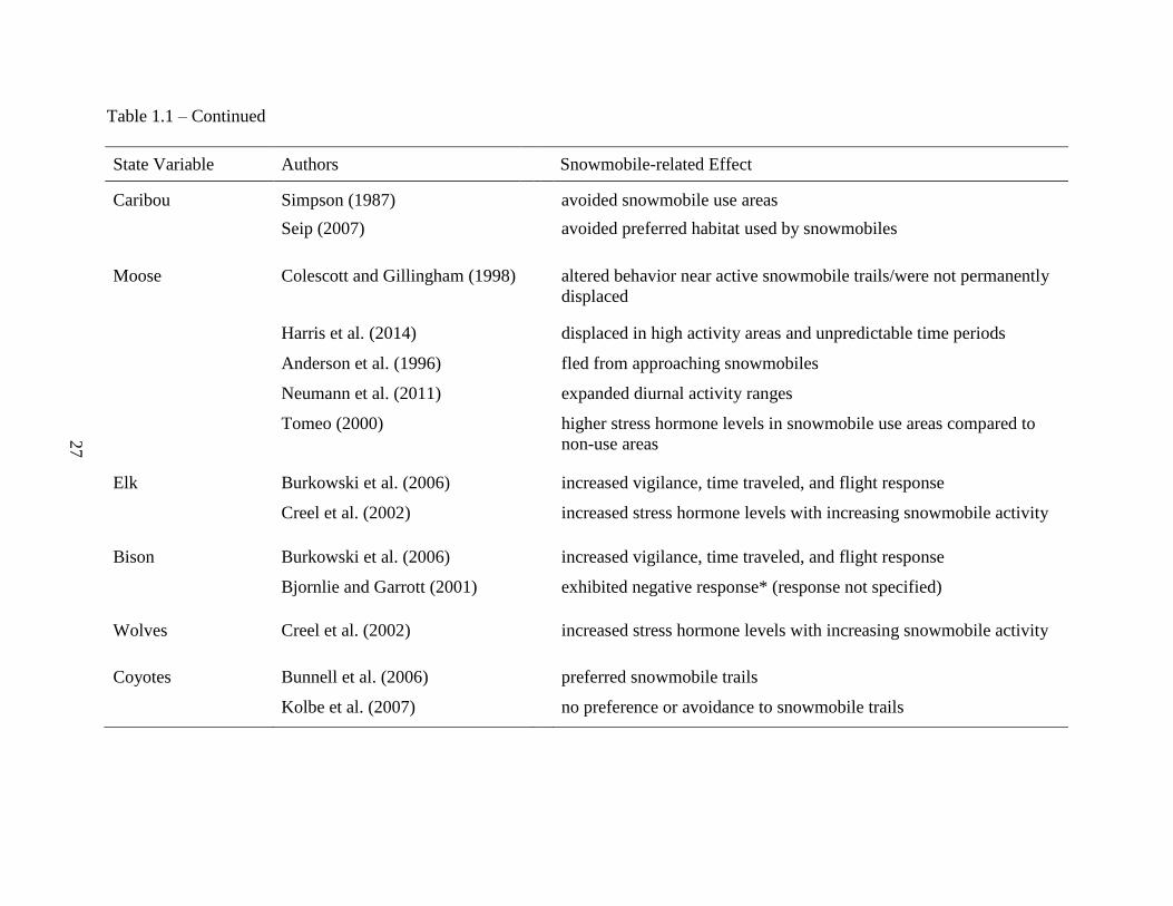
27
Table 1.1 – Continued
State Variable Authors
Snowmobile-related Effect
Caribou Simpson (1987)
avoided snowmobile use areas
Seip (2007) avoided preferred habitat used by snowmobiles
Moose Colescott and Gillingham (1998) altered behavior near active snowmobile trails/were not permanently
displaced
Harris et al. (2014) displaced in high activity areas and unpredictable time periods
Anderson et al. (1996) fled from approaching snowmobiles
Neumann et al. (2011) expanded diurnal activity ranges
Tomeo (2000) higher stress hormone levels in snowmobile use areas compared to
non-use areas
Elk Burkowski et al. (2006) increased vigilance, time traveled, and flight response
Creel et al. (2002) increased stress hormone levels with increasing snowmobile activity
Bison Burkowski et al. (2006) increased vigilance, time traveled, and flight response
Bjornlie and Garrott (2001) exhibited negative response* (response not specified)
Wolves Creel et al. (2002) increased stress hormone levels with increasing snowmobile activity
Coyotes Bunnell et al. (2006) preferred snowmobile trails
Kolbe et al. (2007) no preference or avoidance to snowmobile trails
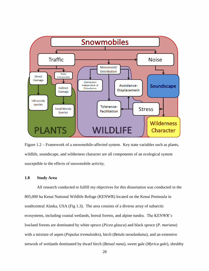
28
Figure 1.2 – Framework of a snowmobile-affected system. Key state variables such as plants,
wildlife, soundscape, and wilderness character are all components of an ecological system
susceptible to the effects of snowmobile activity.
1.8 Study Area
All research conducted to fulfill my objectives for this dissertation was conducted in the
805,000 ha Kenai National Wildlife Refuge (KENWR) located on the Kenai Peninsula in
southcentral Alaska, USA (Fig 1.3). The area consists of a diverse array of subarctic
ecosystems, including coastal wetlands, boreal forests, and alpine tundra. The KENWR’s
lowland forests are dominated by white spruce (Picea glauca) and black spruce (P. mariana)
with a mixture of aspen (Populus tremuloides), birch (Betula neoalaskana), and an extensive
network of wetlands dominated by dwarf birch (Betual nana), sweet gale (Myrica gale), shrubby

29
cinquefoil (Dasiphora floribunda), bog rosemary (Andromeda polifolia), labrador tea (Ledum
palustre), sedges (Carex spp.) and mosses. Temperatures rarely exceed 26°C in the summer or
drop below -18° C in the winter. Annual precipitation on the Kenai Peninsula ranges from 43
cm in the lowlands to 502 cm in the Kenai Mountains.
1.9 Organization of Dissertation
This dissertation is separated into four distinct chapters, each addressing the objectives
stated in Section 1.7. Every chapter includes an abstract summarizing my findings and list of
literature cited at the end of each chapter. In order to emphasize the relevance of peer-reviewed
literature to each chapter, some information provided in this introduction (Chapter 1) is
reemphasized. Following these chapters is an overall discussion of my findings and management
recommendations.

30
Figure 1.3 – Geographical orientation and associated landcover classes of the Kenai National
Wildlife Refuge, Alaska based on 2002 Landsat7 ETM+, USGS DEM, and ground location data
(KENWR Geodatabase).

31
CHAPTER 2
EFFECTS OF SNOWMOBILE TRAFFIC ON THREE SPECIES OF
WETLAND SHRUBS IN SOUTHCENTRAL ALASKA
2.1 Abstract
Snowmobiling is a popular winter activity throughout North America. Although
snowmobiles are an important utility vehicle and serve as a means of outdoor recreation, their
activity causes a number of effects to wildlife and vegetation. Southcentral Alaska is rich with
wetland habitats. Many of these areas are open to snowmobiling where vegetation may be
susceptible to negative impacts. Under undisturbed conditions, vegetation beneath the snow is
protected from harsh winter conditions. However, snowmobile snow compaction can alter this
protective environment, stressing underlying vegetation. I conducted an experiment to determine
how plant height and the number of living and dead stems of three potentially affected wetland
shrub species (dwarf birch; Betula nana, shrubby cinquefoil; Dasiphora floribunda, and sweet
gale; Myrica gale) responded to snowmobile traffic at snow depths of ≥50 cm and <50 cm in
four wetlands on the Kenai Peninsula. I used a Before-After-Control-Impact (BACI) design to
test my hypotheses that snowmobile traffic would have a negative effect on the morphology of
these three species, especially at snow depths <50cm. I established control and two treatment
groups (one with snow depths of ≥50 cm and the other <50 cm). In summer 2011, I tallied living
and dead stems and measured plant height of 150 dwarf birch, 90 shrubby cinquefoil, and 90
sweet gale plants that were individually tagged along three transects. The treated transects were
each traversed 10 times with a snowmobile during winter 2012. I re-measured and recounted all
plants the following summer. Snowmobile traffic at snow depths ≥50 cm reduced the number of
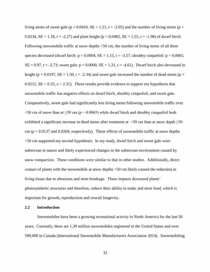
32
living stems of sweet gale (p = 0.0410, SE = 1.21, t = -2.05) and the number of living stems (p =
0.0234, SE = 1.18, t = -2.27) and plant height (p = 0.0482, SE = 1.55, t = -1.98) of dwarf birch.
Following snowmobile traffic at snow depths <50 cm, the number of living stems of all three
species decreased (dwarf birch: p = 0.0004, SE = 1.15, t = -3.57; shrubby cinquefoil: p = 0.0065,
SE = 0.97, t = -2.73; sweet gale: p = 0.0000, SE = 1.21, t = -4.61). Dwarf birch also decreased in
height (p = 0.0197, SE = 1.50, t = -2.34) and sweet gale increased the number of dead stems (p =
0.0212, SE = 0.33, z = 2.31). These results provide evidence to support my hypothesis that
snowmobile traffic has negative effects on dwarf birch, shrubby cinquefoil, and sweet gale.
Comparatively, sweet gale had significantly less living stems following snowmobile traffic over
<50 cm of snow than at ≥50 cm (p = 0.0065) while dwarf birch and shrubby cinquefoil both
exhibited a significant increase in dead stems after treatment at <50 cm than at snow depth ≥50
cm (p = 0.0137 and 0.0204, respectively). These effects of snowmobile traffic at snow depths
<50 cm supported my second hypothesis. In my study, dwarf birch and sweet gale were
subnivean in nature and likely experienced changes in the subnivean environment caused by
snow compaction. These conditions were similar to that in other studies. Additionally, direct
contact of plants with the snowmobile at snow depths <50 cm likely caused the reduction in
living tissue due to abrasions and stem breakage. These impacts decreased plants’
photosynthetic structures and therefore, reduce their ability to make and store food, which is
important for growth, reproduction and overall longevity.
2.2 Introduction
Snowmobiles have been a growing recreational activity in North America for the last 50
years. Currently, there are 1.39 million snowmobiles registered in the United States and over
590,000 in Canada (International Snowmobile Manufacturers Association 2014). Snowmobiling

33
has its benefits for promoting the use and appreciation of wilderness areas and as an important
utility vehicle for trappers, hunters, and others (Simpson 1987). However, snowmobile activity
also causes a variety of effects to wildlife and vegetation during winter when resources are
limited and environmental conditions are severe (Wanek 1971, Neumann and Merriam 1972,
Boyle and Samson 1985, Burkowski et al. 2006, Seip et al. 2007).
Wetlands in southcentral Alaska are important resources for many wildlife species and
are known to contribute to the global uptake of carbon dioxide (Panikov and Gorbenko 1992,
Christensen et al. 1999, Oechel et al. 2000). Additionally, wetlands are also widely used by
snowmobilers for accessing trapping sites and in-holdings, in addition to joy-riding. In winter
when wetland plants are under physical and physiological stress, snowmobile activity could
decrease their productivity and longevity. Such impacts could therefore alter wetland plant
community composition and ecological processes.
I found only two peer-reviewed studies that had specifically examined the effects of
snowmobile traffic on wetland vegetation (Caissie 1991, Keddy et al. 1979). However, there are
several studies that have assessed the effects of snowmobile traffic on other species of plants
(Pesant et al. 1985, Wanek and Schumacher 1975, Wanek 1974, Neumann and Merriam 1972,
Wanek 1971), although these studies are outdated with today’s advancements in snowmobile
technology which now encompasses a variety of makes and models, some being heavier or
lighter, as well as possessing thinner and wider tracks. Based on the lack of sufficient research
and the potential significance of snowmobile impacts, it is important to assess how wetland
vegetation is specifically being affected by this type of activity in order for resource managers to
make informed decisions to limit snowmobile impacts in these important habitats.

34
The direct effects of snowmobiles on vegetation occur when snowmobile skis and tread
come into contact with individual plants (typically woody species) protruding above or just
beneath the snow surface. This results in physical damage to plant tissue inhibiting growth or
causing mortality (Wanek 1971, Neumann and Merriam 1972, Wanek and Schumacher 1975).
Young trees that have been run over by snowmobiles have been found to be significantly
damaged in the form of broken stems or trunks (Wanek 1971). Neumann and Merriam (1972)
observed that over 78% of tree saplings were damaged by a single pass of a snowmobile
compared to 10% of naturally damaged saplings in control transects. Wanek and Schumacher
(1975) found that 93% of Norway spruce were damaged by snowmobile traffic during a year of
low snowfall. Over 8% of those damaged plants died while 45% had received heavy damage.
Shrubs are also known to be heavily damaged by snowmobile traffic (Wanek 1971, Wanek
1974). Such damage generally increases with increasing snowmobile traffic. The direct effects
of snowmobile activity on woody plants could adversely affect their subsequent reproduction,
growth, and longevity.
Snow creates an insulated subnivean environment that is typically warmer than the air
above snow (Marchand 1996). The subnivean environment therefore provides a protection zone
for plants against the harsh winter elements above the snow that may provide temperatures warm
enough for cell division (Kimball and Salisbury 1974). When the subnivean environment is
disturbed, its physical and insulative properties are altered which ultimately stresses the
underlying vegetation. Therefore, indirect effects of snowmobiles can be caused by their
tendency to compact the snow surface, otherwise degrading the subnivean environment.
Pesant et al. (1985) found that temperatures beneath the snow in their experimental area
rarely fell below -1°C at an average depth of 20 cm during undisturbed conditions. Conversely,

35
compaction by snowmobile increased heat conduction to decrease snow temperatures to -6°C at
20 cm. This change in environmental condition led to reductions in soil temperatures that
reduced food reserves stored in plants’ roots which prevented them from growing the following
spring (Bolduc et al. 1977). Wanek (1971) and Neumann and Merriam (1972) found that
temperature gradients and thermal insulation of snow beneath the surface are drastically reduced
by the compaction of snow caused by snowmobiles. Their experiments showed that the specific
gravity of snow doubled below the surface, and tripled at the surface by snowmobile traffic
compared to areas without snowmobile traffic, ultimately increasing thermal conductivity below
and at the surface by four and nine times, respectively (Neumann and Merriam 1972). Changes
in snow structure caused by compaction can also reduce its water holding capacity by 70% near
the surface, and 40% below the surface (Neumann and Merriam 1972). In general, snowmobile
trails melt more slowly than areas without snowmobile compaction, as can be seen widely in
early spring on snowmobile trails. These effects would significantly reduce the ability of snow
to slow runoff and to moderate the effects of thawing during snow melt, as well as affect
vegetative growth and composition (Neumann and Merriam 1972). Similarly, Keddy et al.
(1979) found that most snow compaction occurred after a single pass and treatment areas melted
slower than control areas.
Experiments conducted by Pesant et al. (1985) on the effects of snowmobile traffic on
legume species and forage stands in agricultural fields in Quebec found that snowmobile traffic
retarded early season plant growth and reduced forage yields and legume stands due to decreased
insulation of snow caused by snowmobile snow compaction. Snowmobile use has also been
known to significantly reduce yields of bluegrass (Poa patensis; Foresman et al. 1973) and
alfalfa (Medicago sativa; Wanek 1974) depending on snow conditions. Wanek (1974)

36
demonstrated that early spring flowers were smaller and bog plant species decreased after
snowmobile treatments relative to control plots. Keddy et al. (1979) found that snowmobile
traffic significantly reduced standing crops in old fields in Nova Scotia, Canada, yet marsh plants
were not affected. In other studies conducted in Wisconsin and Maine, Ryerson et al. (1977) and
Whitaker and Wentworth (1972) found that snowmobiling had no negative effects on forage
stands.
Based on the findings of the aforementioned studies, it is clear that plant communities’
susceptibility to damage by snowmobiles depends on the depth of snow on which snowmobiles
travel and the types of landcover where their activity occurs. In areas that have both protruding
vegetation above the snow surface and underlying vegetation below the surface, the direct and
indirect effects of snowmobiles are additive, thus making a more substantial impact on plant
communities. These cumulative impacts can lower plant density and composition (Neumann and
Merriam 1972), reduce productivity and growth (Wanek and Potter 1974, Wanek and
Schumacher 1975), and delay seed germination (Keddy et al. 1979). However, the mixed results
of snowmobile effects on vegetation provide evidence that not all species of plant respond the
same; further, woody species likely respond differently than forbs and grasses.
Until now, no study has considered the effect of snow depth on the vulnerability of
wetland species to snowmobile activity. This information is essential for assessing whether
wetlands subjected to snowmobile activity are threatened and therefore of conservation concern.
The aim of this study was to determine the effects snowmobile traffic has on woody wetland
plants at varying snow depths.
37
2.3 Methods
2.3.1 Hypotheses
Snow depth can play an important role in protecting woody vegetation from damage by
snowmobiles. Marchand (1982) found that snow depths of ≥50 cm provide stable temperatures
to protect underlying vegetation from environmental conditions above the snow regardless of
snow density. Furthermore, snow depths ≥50 cm could also protect taller shrubs from direct
damage by snowmobile traffic. Wetlands, however, are typically at lower elevations where snow
depth may not meet or maintain ≥50 cm of snow over the entire winter.
The KENWR has over 6,500 ha of shrub-dominated wetlands (KENWR Geodatabase)
much of which is accessible to snowmobilers (Fig 1.3). The KENWR Manager is charged with
making decisions that will protect natural resources such as wetlands while allowing access to
snowmobiles. Without sufficient information to reference, KENWR managers over the years
have opened KENWR to snowmobiling only when snow depths are ≥30 cm (R. West and A.
Loranger, KENWR, pers comms.). Knowledge regarding the insulative properties of snow
depths ≥50 cm and the potential for wetland plants to be more susceptible to the effects of snow
compaction at snow depths <50 cm begs the question of whether a snow depth of 30 cm is
sufficient enough to protect vegetation from snowmobile impacts.
The height, number of living stems, and number of dead stems on a given plant are all
good indicators of plant health (Sachs 2006) as well as a measure of potential impacts to direct
and indirect effects of snowmobile traffic. I hypothesized that shrub height and number of living
stems would be significantly reduced after snowmobile traffic and that the impact would be
greater at snow depths <50 cm than snow depths ≥50 cm. Conversely, I expected the number of
dead stems to increase after snowmobile traffic.

38
2.3.2 Sampling Design
I used a Before-After-Control-Impact (BACI) design to test my hypotheses (Smith 2002).
I established three transects 50 m long, 2 m wide, and 1 m apart. I set aside Transect 1 as the
control with no snowmobile traffic and Transects 2 and 3 were set as treatment groups (i.e.,
impact groups). I treated Transect 2 with 10 snowmobile traverses over ≥50 cm of snow and
Transect 3 with 10 snowmobile traverses over <50 cm of snow. Treatments for ≥50 cm of snow
were conducted on 23 January 2012 while treatments for <50 cm of snow were conducted on 17
April 2012. I measured snow depth at 5-m intervals in each transect just before treatment and
then again following treatment. Temperatures between treatments ranged from -33 to 9°C. I
conducted all snowmobile traverses with a 2009 Ski Doo Skandic, an average size model of
snowmobile. The 2009 Skandic has a total width of 1.15 m from ski to ski, a track width of 0.6
m and a dry weight of 326 kg. The rider was approximately 100 kg and traveled at a rate of 2
km/h over treatment groups.
To determine the appropriate sample size for detecting a ≥10% effect size, I conducted an
a priori, balanced one-way ANOVA power analysis in program R (R Core Team 2012). I took
several steps to calculate the power analysis using data obtained from a previous pilot study. I
first generated simulated pre-treatment data based on the mean and variance. Second, I applied a
rate of stem decline for each shrub. I initially set the decline at 5% to represent a natural decline
in the number of stems. I also set a rate of stem decline for post-treatment at a rate of 6 to 80%
to see if the simulation could detect a difference in treatments. Third, I simulated pre-treatment
and post-treatment data and calculated the percent decline for each plant. Fourth, I used a nested
ANOVA based on the percent decline where the fixed effect was the three treatments and the
random effect was the number of sample sites (n = 3). I ran an ANOVA without the fixed effects
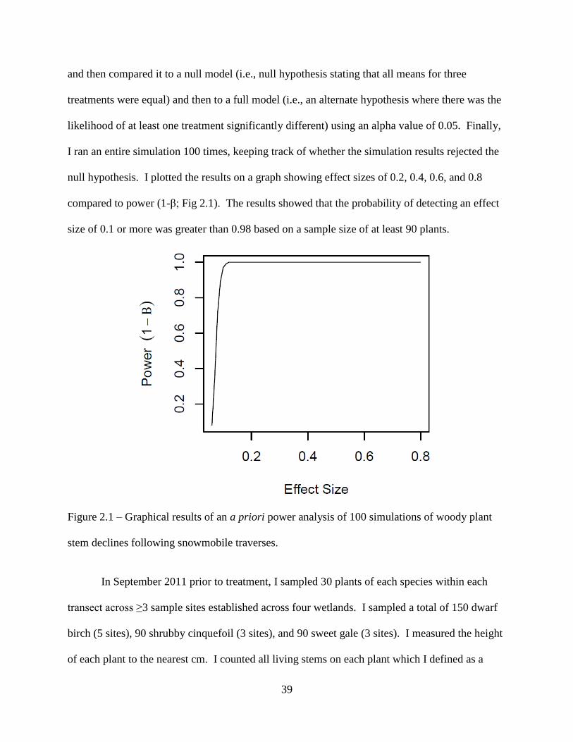
39
and then compared it to a null model (i.e., null hypothesis stating that all means for three
treatments were equal) and then to a full model (i.e., an alternate hypothesis where there was the
likelihood of at least one treatment significantly different) using an alpha value of 0.05. Finally,
I ran an entire simulation 100 times, keeping track of whether the simulation results rejected the
null hypothesis. I plotted the results on a graph showing effect sizes of 0.2, 0.4, 0.6, and 0.8
compared to power (1-β; Fig 2.1). The results showed that the probability of detecting an effect
size of 0.1 or more was greater than 0.98 based on a sample size of at least 90 plants.
Figure 2.1 – Graphical results of an a priori power analysis of 100 simulations of woody plant
stem declines following snowmobile traverses.
In September 2011 prior to treatment, I sampled 30 plants of each species within each
transect across ≥3 sample sites established across four wetlands. I sampled a total of 150 dwarf
birch (5 sites), 90 shrubby cinquefoil (3 sites), and 90 sweet gale (3 sites). I measured the height
of each plant to the nearest cm. I counted all living stems on each plant which I defined as a
40
stem that was green and/or flexible, had the presence of leaves and/or terminal flowers, or
fruiting bodies branching from the main stem. I also counted the number of dead stems on each
plant. I marked each plant with a color-coded zip-tie and an identification number to ensure that
the same plants were counted the following summer. In August 2012, I re-measured the height
of all marked plants and recounted all living and dead stems
2.3.3 Statistical Analysis
The primary aim of my study was to determine the effects of snowmobile traffic at
varying snow depths on three wetland shrub species measured by the parameters of: 1) plant
height, 2) number of living stems, and 3) number of dead stems. Plant height and log-
transformed living stem counts for all species were normally distributed. For these data I tested
a set of a priori general linear mixed effects models (GLMM) using the “nlme” package in
program R (Pinheiro et al. 2013). Dead stem data were not normally distributed even when
transformed and were zero-inflated and overdispersed when comparing the variance to the mean.
Because these data were counts and over dispersed, they fit a zero-inflated negative binomial
distribution. Therefore, I fit zero-inflated negative binomial generalized linear mixed models
using the ‘glmmADMB’ package in program R (Skaug et al. 2012).
I built my model based on the predictors of ‘Time’ (i.e., pre- and post-treatment) and
‘Treatment’ (i.e., Control, Transect 2, and Transect 3). In BACI study designs, a significant
effect of ecological impacts appear via the interaction between treatment and time; thus I tested
for an effect of snowmobile traffic at varying snow depths on the three measured parameters by
including the interaction between ‘Treatment’ and ‘Time (Eq. 2.1).’ All models included the
random effects of sample site (Eq. 2.1). Equation 2.1 is the general linear mixed-effects model I
used to determine the effects of snowmobile traffic on wetland shrubs:

41
(2.1) yi = b0 + b1(Time) + b2(Treatment) + b3(Time*Treatment) + Site + ei
To determine whether there was a difference of snowmobile effects between snow depths, I used
a Welch 2-sample t-test for normally distributed data and a non-parametric Mann-Whitney U test
for data that were not normally distributed. Model and test results with p ≤ 0.05 (α = 0.05) were
considered significant.
2.4 Results
2.4.1 Snow Compaction
Average snow depth for Transect 2 pre-treatment was 52 cm (sd = 9.71, n = 28).
Following snowmobile treatment, the snow depth for Transect 2 was 32 cm (sd = 7.94). Average
snow depth for Transect 3 before snowmobile treatment was 34 cm (sd = 8.02, n = 28). Snow
depth for Transect 3 following treatment was 24 cm (sd = 7.04). Snowmobile snow compaction
resulted in a 38 and 29% reduction in snow depth for Transects 2 and 3, respectively.
2.4.2 Vegetation Response at Snow Depths ≥50 cm
The heights of dwarf birch (p = 0.0582, SE = 1.55, t = -1.98), shrubby cinquefoil (p =
0.4485, SE = 2.87, t = -0.74), and sweet gale (p = 0.3628, SE = 1.40, t = -0.91) height were not
affected by snowmobile traffic at snow depths ≥50 cm when compared to pre-treatment heights
and control following snowmobile traffic (Table 2.1, Fig 2.2).

42
Table 2.1 – Model estimates of the response of plant height measured from three wetland shrub
species to snowmobile traffic and associated p-values when compared to control and pre-
treatment conditions at snow depths ≥50 cm and <50 cm.
Treatment Estimate Std Error t-value p-value
Dwarf Birch
Intercept 30.54 1.79 17.02 0.0000**
≥50 cm -3.06 1.55 -1.98 0.0582
<50 cm -3.50 1.50 -2.34 0.0197*
Shrubby Cinquefoil
Intercept 52.21 2.69 19.4 0.0000**
≥50 cm -2.18 2.87 -0.74 0.4485
<50 cm -1.86 2.87 -0.65 0.5184
Sweet Gale
Intercept 27.77 1.24 22.4 0.0000**
≥50 cm -1.28 1.40 -0.91 0.3628
<50 cm -1.64 1.40 -1.17 0.2411
* Significant at α = 0.05
** Significant at α = 0.01

43
Figure 2.2 – Mean plant height and 95% confidence intervals from three woody shrub species
(dwarf birch, shrubby cinquefoil, and sweet gale) in comparison between control and treatment
plots (Transect 2 is ≥50 cm snow depth; Transect 3 is <50 cm snow depth) before (Pretreatment)
and after (Post-treatment) 10 snowmobile traverses.
The number of living stems of dwarf birch (p = 0.0234, SE = 1.18, t = -2.27) and sweet
gale (p = 0.0410, SE = 1.21, t = -2.05) were significantly lower following snowmobile traffic
when compared to pre-treatment and control while shrubby cinquefoil did not exhibit a
significant difference (p = 0.2134, SE = 0.97, t = -1.25) in the number of living stems following
treatment when compared to pre-treatment and control (Table 2.2; Fig 2.3).
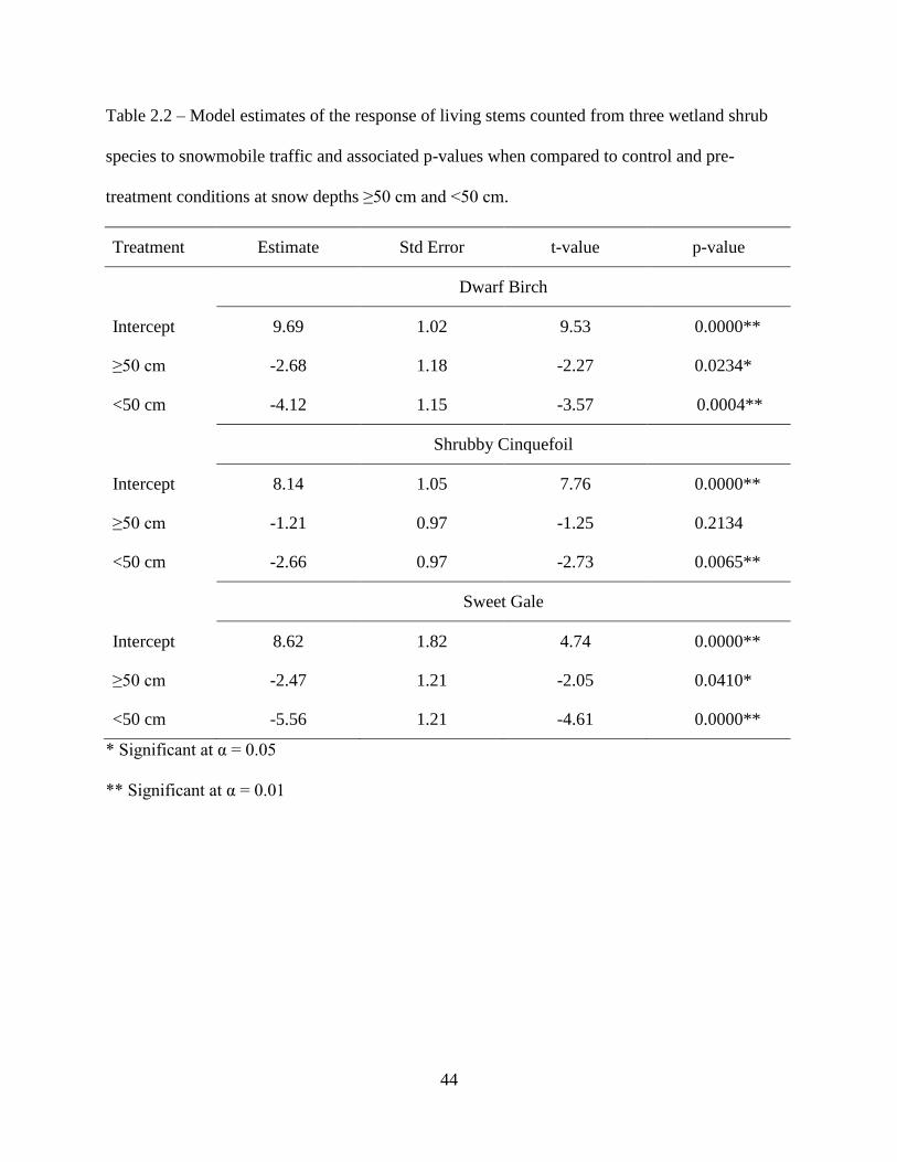
44
Table 2.2 – Model estimates of the response of living stems counted from three wetland shrub
species to snowmobile traffic and associated p-values when compared to control and pre-
treatment conditions at snow depths ≥50 cm and <50 cm.
Treatment Estimate Std Error t-value p-value
Dwarf Birch
Intercept 9.69 1.02 9.53 0.0000**
≥50 cm -2.68 1.18 -2.27 0.0234*
<50 cm -4.12 1.15 -3.57 0.0004**
Shrubby Cinquefoil
Intercept 8.14 1.05 7.76 0.0000**
≥50 cm -1.21 0.97 -1.25 0.2134
<50 cm -2.66 0.97 -2.73 0.0065**
Sweet Gale
Intercept 8.62 1.82 4.74 0.0000**
≥50 cm -2.47 1.21 -2.05 0.0410*
<50 cm -5.56 1.21 -4.61 0.0000**
* Significant at α = 0.05
** Significant at α = 0.01

45
Figure 2.3 – Mean number of living stems and 95% confidence intervals from three woody shrub
species (dwarf birch, shrubby cinquefoil, and sweet gale) in comparison between control and
treatment plots (Transect 2 is ≥50 cm snow depth; Transect 3 is <50 cm snow depth) before
(Pretreatment) and after (Post-treatment) 10 snowmobile traverses.
The number of dead stems on dwarf birch (p = 0.3043, SE = 0.25, z = -1.03) and shrubby
cinquefoil (p = 0.9973, SE = 0.24, z = 0.00) did not increase following snowmobile treatments
although dead stems were more prevalent on sweet gale plants (p = 0.0179, SE = 0.36, z = 2.37)
when compared to pre-treatment counts and those of control (Table 2.3; Fig 2.4).

46
Table 2.3 – Model estimates of the response of dead stems counted from three wetland shrub
species to snowmobile traffic and associated p-values when compared to control and pre-
treatment conditions at snow depths ≥50 cm and <50 cm.
Treatment Estimate Std Error z-value p-value
Dwarf Birch
Intercept 0.90 0.26 3.43 0.0006**
≥50 cm -0.26 0.25 -1.03 0.3043
<50 cm 0.21 0.24 0.88 0.3800
Shrubby Cinquefoil
Intercept 1.46 0.13 11.39 0.0000**
≥50 cm 0.00 0.24 0 0.9973
<50 cm 0.50 0.27 1.87 0.0615
Sweet Gale
Intercept 0.46 0.17 2.73 0.0063**
≥50 cm 0.86 0.36 2.37 0.0179*
<50 cm 0.75 0.33 2.31 0.0212*
* Significant at α = 0.05
** Significant at α = 0.01

47
Figure 2.4 – Mean number of dead stems and 95% confidence intervals from three woody shrub
species (dwarf birch, shrubby cinquefoil, and sweet gale) in comparison between control and
treatment plots (Transect 2 is ≥50 cm snow depth; Transect 3 is <50 cm snow depth) before
(Pretreatment) and after (Post-treatment) 10 snowmobile traverses.
2.4.3 Vegetation Response at Snow Depths <50 cm
The height of dwarf birch plants decreased (p = 0.0197, SE = 1.50, t = -2.34) following
snowmobile traffic at snow depths <50 cm when compared to pre-treatment and control (Table
2.1, Fig 2. 2). Conversely, the height of shrubby cinquefoil (p = 0.5184, SE = 2.87, t = -0.65)
and sweet gale (p = 0.2411, SE = 1.40, t = -1.17) plants were not affected (Table 2.1, Fig 2.2).

48
Dwarf birch (p = 0.0004, SE = 1.15, t = -3.57), shrubby cinquefoil (p = 0.0065, SE = 0.97, t = -
2.73), and sweet gale (p = 0.0000, SE = 1.21, t = -4.61) all decreased in the number of living
stems following snowmobile traffic at <50 cm snow depth (Table 2.2, Fig 2.3). Dwarf birch (p =
0.3800, SE = 0.24, z = 0.88) and shrubby cinquefoil (p = 0.0615, SE = 0.27, z = 1.87) did not
increase in the number of dead stems following snowmobile treatments (Tables 2.3, Fig 2.4).
However, sweet gale plants did show an increase in the number of dead stems (p = 0.0212, SE =
0.33, z = 2.31) when compared to pre-treatment and control (Table 2.3, Fig 2.4).
2.4.4 Comparison between Treatment Groups
Comparatively, the effects of snowmobile traffic at snow depths <50 cm on the height of
all three species were not significantly different from that at snow depths ≥50 cm (dwarf birch: p
= 0.121; shrubby cinquefoil: p = 0.8727; sweet gale: p = 0.9266). Sweet gale plants experienced
more dieback (p = 0.0065) following snowmobile traffic over <50 cm of snow than that of snow
depths ≥50 cm but such effects were not apparent for living stems of dwarf birch (p = 0.1624)
and shrubby cinquefoil (p = 0.0710). Conversely, dwarf birch (p = 0.0137) and shrubby
cinquefoil (p = 0.0204) both showed more dead stems after snowmobile traffic over <50 cm of
snow than ≥50 cm while sweet gale did not (p = 0.2424).
2.5 Discussion
These results support my hypothesis that snowmobile traffic has negative effects on
dwarf birch, shrubby cinquefoil, and sweet gale, three common woody shrub species growing in
wetlands on the Kenai Peninsula. Dwarf birch and sweet gale exhibited negative effects to
snowmobile traffic over both snow depths while shrubby cinquefoil appeared to be more
resistant to the effects of snowmobile traffic at snow depths ≥50 cm. The effects of snowmobile

49
traffic at snow depths <50 cm were significantly more than those at snow depths ≥50 cm,
supporting my second hypothesis.
During this study, dwarf birch and sweet gale did not protrude above the snow pack at
either depth prior to snowmobile traverses and were therefore subnivean in nature. I noted that
plants of both species remained within the subnivean layer following snowmobile traverses over
snow ≥50 cm in depth. Although I did not measure changes in the subnivean environment, other
studies have found that snow compaction (and increased snow density) caused by snowmobiles
does increase thermal conductivity, thereby reducing the snow’s insulative properties (Wanek
1971, Neumann and Merriam 1972, Bolduc et al. 1977, Pesant et al. 1985). These changes to the
subnivean environment are known to retard growth and reduce the densities of subnivean plants
(Foresman et al. 1973, Wanek 1974, Pesant et al. 1985).
Since my study’s design and results were similar to those mentioned above, the results
support that the compaction of snow following snowmobile traverses over snow ≥50 cm in depth
likely changed the subnivean environment enough to reduce the number of living stems of dwarf
birch and sweet gale. Dwarf birch is known to be fairly resistant to cold temperatures and
frosting (de Groot et al. 1997) and my results suggest that changes to the subnivean environment
in my experiment could have exceeded the limits of this plant’s ability to resist colder
temperatures below the surface. Further study on this subject could support this hypothesis.
All three shrub species were negatively affected by snowmobile traffic at snow depths
<50 cm. Many shrubby cinquefoil plants were found protruding above the snow pack at this
snow depth prior to treatment and therefore experienced direct contact with the snowmobile.
Conversely, dwarf birch and sweet gale plants remained buried in the snow pack prior to
snowmobile traverses yet many plants of both species were found protruding above the snow

50
pack following treatment, suggesting that dwarf birch and sweet gale plants also came in contact
with the snowmobile during treatment. This is likely the reason why all three species had
significant losses of living stems (i.e., dieback). I noted during the summer following treatments
that plants of shrubby cinquefoil within Transect 3 had noticeable abrasions on the main stems,
and all three species had stems that were broken. Several studies have found that woody plants
that protrude above the snow pack or remain just below the surface experience significant
damage from snowmobile traffic in the form of broken stems which is known to inhibit growth
(Wanek 1971, Neumann and Merriam 1972, Wanek and Schumacher 1975). My results are
consistent with these studies.
The combination of direct and indirect effects of snowmobile traffic on these three
species may have broader ecological effects. Dwarf birch serves as an important browse species
for moose during winter (Renecker and Schwartz 1997, Collins 2002). Moose have even been
observed foraging on dwarf birch in place of willow species (Salix sp.) due to its similar
nutritional content but lower levels of tannins (Collins 2002). Shrubby cinquefoil is a prolific
wetland species and is important for maintaining wetland substrates for the establishment of
other wetland species (Ladyman 2003). Sweet gale has also been known as a browse species for
moose but also serves as an important plant for gas exchange and nitrogen fixation in wetland
communities (Schwintzer 1979). The impacts of snowmobiles to these three species decrease
photosynthetic structures and therefore, reduce plants’ ability to make and store food which is
important for growth, reproduction and overall longevity. Should snowmobile traffic occur over
a larger area, over a longer period of time, and more frequently than what I tested, the possibility
of significant changes to wetland communities and impacts to wildlife are conceivable.
51
CHAPTER 3
TEMPORAL AND SPATIAL VARIATION OF A WINTER SOUNDSCAPE IN ALASKA
3.1 Abstract
Sound is an intrinsic component of ecosystems and studies have shown that sound plays a
significant role in how plants and animals interact with each other and with their surroundings.
The same is true for human-wildlife interactions. Soundscapes vary temporally and across
space. Winter possesses unique seasonal soundscape attributes because of a substantial decrease
in wildlife vocalizations (biophony), an increase in wind events (geophony), and motorized noise
from winter recreation like snowmobiling (anthrophony). I introduce a fourth soundscape
component, silence, as an additional and significant attribute of winter soundscapes. My
objectives were to quantify and visualize the temporal and spatial variation of these winter
soundscape components. I sampled 62 locations across KENWR between December 2011 and
April 2012. I recorded ambient sounds for one minute every 30 mins. I quantified the power
spectral density (i.e., soundscape power) within 1 kHz frequency intervals of spectrograms for
each sound recording using the Remote Environmental Assessment Laboratory. I identified the
sounds of 59,597 sound recordings by ear and used those sound files for my analysis. I
visualized the temporal variation (hourly and monthly) of all soundscape components and
generated spatially explicit predictive models of each using machine learning algorithms
(stochastic gradient boosting; TreeNet). Silence was the most prevalent soundscape component
making up 65% of all recordings and occurring predominantly at night. Anthrophony, biophony,
and geophony were all more prevalent during the day. Anthrophony and biophony had similar
temporal patterns over monthly time frames with April having the highest average soundscape

52
power (biophony: n = 137, mean = 0.149, sd = 0.556; anthrophony: n = 991, mean = 0.354, sd =
0.470). Geophonic soundscape power was highest during February (n = 5104, mean = 0.437, sd
= 0.466) and maintained relatively the same power over March (n = 2573, mean = 0.242, sd =
0.408, 95% CI [0.236, 0.249]) and April (n = 783, mean = 0.260, sd = 0.411, 95% CI [0.248,
0.273]). January was the quietest month of winter. Spatially, biophony was predicted further
from urban areas and closer to deciduous forest and rivers. Anthrophony occurred primarily
closer to urban areas and rivers and further from lakes. Rivers were likely corridors for both
vocal wildlife and snowmobile activity. Geophony occurred further from conifer forest and
urban areas and at high elevations. Although silence was recorded at 95% of my sound stations,
it primarily occurred further from rivers and shrubland and closer to or within areas of barren
land. Although my quantification of biophony, anthrophony, geophony, and silence were based
on a frequency of 1-11 kHz, my results shed light on the temporal and spatial variation of
winter’s soundscape components, providing evidence that silence at this frequency range is a
significant part of winter soundscape ecology.
3.2 Introduction
The emergent properties of ecosystems extend beyond that which can be seen. Plants and
animals perceive and interact with their environment using all their senses (Kare 1970, Doty
1976, Wells and Lehner 1978, Nolte et al. 1994, Voigt et al. 2008) and therefore attention should
be given to these interactions to have a more holistic understanding of their roles in ecological
processes. Sound is an intrinsic component of ecosystems and studies have shown that sound
plays a significant role in how plants and animals interact with each other and with their
surroundings (Retallack 1973, Popper and Fay 1980, Hongbo et al. 2008). However, measures
of sound in ecosystems have been primarily focused on small temporal and spatial scales. The
53
field of soundscape ecology focuses its attention on the broader ecological significance of sound
in the landscape (Pijanowski et al. 2011) and landscape-scale soundscape research is proving
useful in assessing the way wildlife interact with their environment (Tucker et al. 2014). The
study of sound as an emergent property of ecosystems over extended periods of time and across a
larger spatial extent contributes to a broader understanding of sound’s role in the environment.
There are three general components to a soundscape: biophony, geophony, and
anthrophony (Krause 1998, Krause 2001, Krause 2002, Qi et al. 2008, Pijanowski et al. 2011).
All sounds made by animals (other than humans) like bird and frog songs make up biophony.
All sounds made by geophysical phenomena such as rain, wind, and flowing water make up
geophony and all human-made sounds like those made by vehicle traffic, airplanes, and ATVs
are anthrophony. Here I introduce a fourth component to the soundscape: silence, or what I
define as no detectable signal by a receiver. Although perhaps rare, I postulate that in certain
wild places during certain times of the day and especially during the winter season there are
periods when animals do not call, wind does not blow, and human activity cannot be heard. I
realize this phenomenon is a matter of a receiver’s sensitivity to sound (e.g., threshold of sound
detection by a microphone or animals hearing) but I will later confirm that, based on my
equipment and the analysis I conducted, silence does exist and can be quantified.
Biophony, geophony, and anthrophony all produce detectable and perceivable signals to
that of a receiver (e.g., an animal’s ear). These signals are interpreted by the receiver to elicit a
physiological and behavioral response (Westman and Walters 1981). Wildlife has adapted to the
natural variation in the soundscape over millions of years. Several hypotheses have attempted to
explain how wildlife use and interpret their sonic environment based on their physical,
behavioral, and cognitive adaptations (see Farina 2014 for a review). In particular, Krause’s
54
(1987, 2012) Spectral Niche Hypothesis suggests that vocal species have evolved the ability to
vocalize within a specific frequency band width (i.e., spectral niche) where their calls can be
distinguished from that of other species in order to maximize their intentions. In this case, sound
can serve as a proxy for determining the level of biodiversity of an area, measured by the number
of occupied acoustic frequencies.
Sound generally serves as a means of communication between individuals, detecting
predators, prey, or competitors (Quinn et al. 2006, Slabbekoorn and Ripmeester 2008, Barber et
al. 2010), or locating suitable habitats or territories (Slabbekoorn and Smith 2002, Wood and
Yezerinac 2006, Barber et al. 2010). Natural soundscapes maintain these relationships and
interactions which allows communication and interpretation to occur unimpeded. When
anthrophony is introduced to a natural soundscape, significant changes can occur in the sonic
environment which can indicate degradation of natural systems (Stone 2000, Dooling and Popper
2007, Habib et al. 2007, Krause et al. 2011, Francis et al. 2012, Ortega 2012, Ortega and Francis
2012). Because of the role sound plays in natural systems and the impacts human activity can
have, conservation efforts must be taken to preserve soundscapes as an inherent property and
valuable environmental resource (Dumyahn and Pijanowski 2011). For this to occur,
conservation biologists and soundscape ecologists should have an understanding of the spatial
and temporal context of sound within these threatened environments.
Soundscapes vary temporally and spatially. Much like that of a symphony, the spring
and fall chorus could be considered the forte of the soundscape while winter would be the piano.
Similarly, soundscapes including urban environments have a different sound configuration than
soundscapes in rural or wilderness areas (Joo et al. 2011). Much of the research in soundscape
ecology has been conducted during the most active acoustic time periods, especially in spring,
55
summer, and fall (Krause and Gage 2003, Joo et al. 2011, Pieretti et al. 2011, Gage and Axel
2014). However, winter possesses unique soundscape attributes.
During winter in northern latitudes, the diversity of wildlife is reduced by the fall
migration southwards. The reduction of daylight hours and the decrease in temperature also
reduce the activity and associated sounds of wildlife that remain. Geophony also changes. The
babbling and rush of water is halted by the freezing of rivers and streams. The impacting sound
of rain falling on leaves, water, and the earth’s surface is transformed into the soft muffle of
falling snow. Even the presence of snow on the ground is known to reduce the propagation of
sound in the landscape (Nicolas et al. 1985). Wind is also strongest during winter due to the
increase in temperature gradients. Human activity is reduced and altered by winter’s influences.
However, in some areas, motorized noise from airplanes and winter recreational vehicles like
snowmobiles is still prevalent. Because of the lack of research on winter soundscapes, their
unique attributes, and the potential for anthrophony to impact the natural sonic environment, the
aim of this study was to capture and describe variations in the winter soundscape of a subarctic
ecosystem over space and time.
3.3 Methods and Materials
3.3.1 Sample Design
3.3.1.1 Spatial Sampling
I partitioned KENWR into six spatially explicit regions. I established a permanent
sample site within each region. To maximize my spatial sampling, I established a mixed number
of temporary sample sites distributed throughout accessible areas of each region. Accessibility
throughout much of KENWR in winter was limited to roads, snowmobile trails, rivers, and lakes
accessible by snowmobile or ski plane. I sampled a total of 62 locations within a variety of
56
environments, including urban areas, wetlands, mixed coniferous forests, deciduous forests,
lakes, rivers, streams, alpine, and glacier. I recorded the latitude and longitude (decimal degrees)
of each sample site with a Geographical Positioning System (WGS 1984 coordinate system)
which associated each sound record to a spatially explicit location in the landscape (Fig 3.1).
3.3.1.2 Sound Sampling and Data Acquisition
I recorded ambient sounds from December 2011 to April 2012 using Song Meter SM2TM
autonomous recorders (Wildlife Acoustics, Inc, Massachusetts). I scheduled my song meters to
record for 1 min at 30-min intervals for a total of 48 samples per day. I recorded in monaural at
16 bits in a Waveform Audio File Format (WAV) at a frequency of 22,050 Hz for a total useable
frequency range of 11 kHz. I stored my sound data onto two, 2-GB SD cards and transferred to a
2-TB hard drive in the lab. Due to the battery life in cold temperatures (-35 to 0°C), I visited
each permanent sound recorder every 7-10 days to replace batteries and SD cards. Temporary
sound recorders sampled ambient sounds for 10 days, at which point I exchanged the SD cards
and batteries and redeployed the recorder to a new location.
I uploaded and archived a total of 120,500 sound files into the Remote Environmental
Assessment Laboratory’s (REAL) digital sound library located at Michigan State University
(www.real.msu.edu) as described by Kasten et al. (2012). The REAL sound library stores sound
recordings, computes and displays soundscape metrics, and enables users to access and query
soundscape information for analysis. Kasten et al. (2012) provides details on how REAL
uploads, processes, archives, and accesses sound recordings and derives soundscape metrics.

57
Figure 3.1 – Spatial distribution of sound recording stations in relation to a grid partition
separating the Kenai National Wildlife Refuge study area into six sample areas.

58
Each type of sound present in the environment emits its own frequency and recordings of
these sound frequencies and their energy can be visualized in a spectrogram, where frequency is
indicated on the Y-axis and time on the X-axis. The energy of a sound within a spectrogram is
indicated by the brightness of the color representing that sound. Louder sounds (i.e., sounds with
more energy) have brighter, more intense colors. This sound energy is termed Power Spectral
Density (PSD), as developed by Welch (1967), a measure of soundscape power expressed in
watts/kHz. In order to quantify the PSD within each spectrogram and isolate the frequencies of
soundscape components, spectrograms were partitioned into 1 kHz frequency intervals. Matlab
(2006) code was developed to compute PSD values. PSD values were standardized across 10
frequency intervals (1-11 kHz) and sound recordings by calculating a vector normalization of
PSD values (nPSD) between 0 and 1 (Kasten et al. 2012). The nPSD values were computed in
Matlab prior to translating to PHP scripting language for the REAL web site. I term this nPSD
value as soundscape power (Gage and Axel 2014; Fig 3.2).

59
Figure 3.2 – Example of a spectrogram generated in the Remote Environmental Assessment
Laboratory digital sound library of a recording of light wind (wash of light blue in the 1 kHz
band width at 0-30 secs), a boreal chickadee chirping (intermittent light blue points in the 2-3
kHz band widths at 5-20 secs), and a red squirrel chattering (light blue series of lines between the
1-6 kHz band widths at 35-45 secs). Yellow lines indicate separations into 1 kHz frequency
band widths with their associated normalized power spectral density values (watts/kHz)
calculated from Welch (1967) algorithm.
3.3.1.3 Discriminating Soundscape Components
In order to describe what I identified as four soundscape components (biophony,
anthrophony, geophony, and silence), it was important to discriminate these components from
one another. Gage and Axel (2014) found that most anthrophony and a few biophonic sounds
(e.g., the calls of the common loon (Gavia immer) and Canada goose (Branta canadensis
maxima)) occur in the 1-2 kHz range, whereas passerines, such as the American robin (Turdus
60
migratorius) and smaller species like the common yellowthroat (Geothlypis trichas) within their
study, occurred between 3-6 kHz. The higher frequencies (>6 kHz) were occupied by insects.
Geophony was generally found throughout all frequency intervals (1-11 kHz). Gage and Axel’s
(2014) study was conducted during April through October in Michigan. After initial analysis of
sound data I collected from a pilot project over the winter of 2010-2011, I found that my suite of
organisms, although much different, had similar variation in the frequencies they occupied.
Because biophony, anthrophony, and geophony overlapped in their frequencies, I could not rely
on an automated system to discriminate and precisely describe KENWR’s winter soundscape.
To overcome this obstacle, I listened to a subset of my sound recordings. Due to the
extent of my data set, I had to make this process as efficient as possible. The REAL website
allows the user to query and download any amount of data by using a number of options. I
filtered sound data using soundscape power by frequency. To determine what sound frequency
intervals most sound sources occupied, I listened to and identified the sounds recorded within
270 random sound files taken from 17 sound stations. I downloaded all data from each sound
file from the REAL sound library where a spreadsheet was produced providing the soundscape
power values for each sound file across 10 frequency band widths. Each identified sound was
added to the appropriate record. I then ran a linear discriminate function analysis (LDFA) using
the MASS package in R (R Development Core Team 2012) for each frequency interval and I
produced a prediction table indicating how well each interval discriminated sound sources from
one another.
I found that anthrophonic sound sources including automobiles, airplanes, and
snowmobiles, were not discriminated from one another because their soundscape power
overlapped one another within each frequency interval. However, all anthrophonic sound

61
sources identified had predominantly high soundscape power values in the 1-2 kHz range.
Silence was discriminated from all other sound events 100% of the time within the 4-5 kHz band
width and when adding the total soundscape energy across all frequency intervals. Several
biophonic sounds, like those made by ravens (Corvus corax) and great horned owls (Bubo
virginianus), occur at low frequency levels and, consequently, were not easily discriminated
from anthrophony. Other biophonic sounds made by the high frequency vocalization of
common redpolls (Carduelis flammea) and chickadees (Poecile sp.) were difficult to fully
discriminate from silence, perhaps due to the quietness of the recordings. Wind was the most
confounding sound event for all frequency band widths. Wind’s soundscape power values
overlapped anthrophony and silence considerably.
After evaluating how well I could discriminate specific sound sources by frequency
interval, I conducted an additional LDFA for each soundscape component. I grouped
automobiles, airplanes, and snowmobiles into anthrophony, ravens and chickadees as biophony,
wind as geophony, and sound files with no detected signal as silence. The high soundscape
power values within the 1-2 kHz interval had the highest percentage of correctly discriminated
anthrophony with the least amount of overlap from other soundscape components (Table 3.1).
Most biophony was discriminated by two frequency intervals (1-2 and 6-7 kHz),
indicating some organisms call at lower frequencies while others higher. One-hundred percent
of the sound files I identified as silence were correctly discriminated within the 4-5 kHz interval
and when adding soundscape power values across all intervals (i.e., total energy). Geophony
was correctly discriminated from other sound files 70% of the time within the 1-2 kHz interval
(Table 3.1). The LDFA provided sufficient information to enable selective queries of sound data
archived in REAL.

62
Table 3.1 – Percentage of correctly discriminated sounds within each soundscape component
calculated by a linear discriminate function analysis (LDFA) using 270 sound files recorded
from 17 sound stations. All sounds within each sound file were identified by ear. Number in
parentheses indicates the percentage of wind events misidentified as anthrophony and silence by
the LDFA.
kHz Interval Anthrophony Biophony Geophony Silence
1-2 71 (6) 13 70 98 (24)
2-3 77 (17) 0 41 99 (41)
3-4 75 (34) 0 29 99 (37)
4-5 75 (37) 0 26 100 (37)
5-6 73 (34) 0 27 99 (39)
6-7 68 (30) 13 31 98 (39)
7-8 79 (40) 0 23 96 (37)
8-9 79 (39) 0 23 90 (39)
9-10 79 (34) 0 26 88 (26)
10-11 79 (34) 0 26 88 (40)
Total Energy 75 (36) 0 24 100 (40)
I queried all sound files with a soundscape power value of ≥0.8 in the 1-2 kHz interval to
acquire anthrophonic sound events. This query produced 19,813 sound files. To capture higher
frequency biophony, I searched all sound files with a total energy soundscape power ≥1.8 and
soundscape power in the 1-2 kHz interval which was <0.4. This query was intended to capture
sound events with high soundscape power in the higher frequencies (e.g., passerine calls other
than corvids) and attempt to eliminate sound events in lower frequencies with high soundscape

63
power. This query produced 1,826 total files. The LDFA I conducted indicated silence sound
files were effectively identified using high values of total soundscape power but a high
percentage of wind events were also misclassified using this discriminate category. I made my
search for silence sound files more efficient by using an alternative search criterion. I used the
ksax code for sound files identified as silence. Ksax codes are assigned to each sound file and
sound files with the same attributes of soundscape power are given the same ksax code (Kasten
et al. 2012). Therefore, sound files I identified as having no detected signal had the same ksax
code. I queried all sound files with the ksax code starting with %jig with a soundscape power in
the 1-2 kHz interval <0.6. This latter filter was used to attempt to eliminate any wind events.
This final query produced 37,958 sound files of silence. A sound technician listened to and
verified the identity of all 59,597 sound files, 49.5% of the total sound records I recorded over
the entire winter.
3.3.2 Soundscape Analysis
I summarized and graphed soundscape power metrics from the 59,597 recordings in
which soundscape elements had been identified using Minitab v16 (Minitab 16 Statistical
Software, 2010). I treated the sound records for each station as a temporal and spatial sample of
the winter soundscape and were therefore summarized as the mean soundscape power for all of
winter and the entire study area. I calculated and visualized the amount of soundscape power
within each frequency interval for each soundscape component. I also visualized the temporal
variation of each soundscape component over hourly and monthly time frames. I conducted a
Pearson correlation test to determine how soundscape components were significantly temporally
correlated with one another. I calculated a one-way ANOVA and 95% confidence interval (CI)
to determine whether there was a significant difference of soundscape power for each

64
soundscape component between months. Additionally, I calculated the proportional contribution
of each soundscape component to the winter soundscape, as well as the proportion of specific
biophonic and anthrophonic sound sources present in my recordings. I determined there to be a
significant correlation if p-values were less than α = 0.05. I used a Bonferroni correction for
calculating the differences between months.
3.3.3 Building Spatially Explicit Predictive Models and Mapping
Soundscape Components
I used machine learning to model each soundscape component. Machine-learning
algorithms (e.g., boosted regression trees, CART, RandomForests, TreeNet) have become
increasingly useful tools for quantifying the spatial distribution of plants and animals (Guisan
and Zimmermann 2000, Elith et al. 2006, Prasad et al. 2006, Cutler et al. 2007, Craig and
Huettmann 2009, Drew et al. 2011). My hypothesis was that sound, in a spatial context, could
also be modeled using these tools. These algorithms do not require a priori assumptions
regarding explanatory variables which allow the models to be more flexible than traditional
generalized linear or additive models.
I used stochastic gradient boosting (TreeNet; Salford Systems, Inc., San Diego, CA) to
build predictive models of each soundscape component using a weighted average (WA) of
soundscape power for each sound station. Because each sound station and each sound
component had a different number of sound records, I weighted the average amount of
soundscape power for all recordings of each soundscape component by its proportion to the total
number of recordings (59,597). The WA of each soundscape component at each sound station
had a latitude and longitude associated with it. I input the coordinates of each sound station into
ArcGIS 10.2.1 and overlaid those locations with 11 to 17 associated environmental layers using
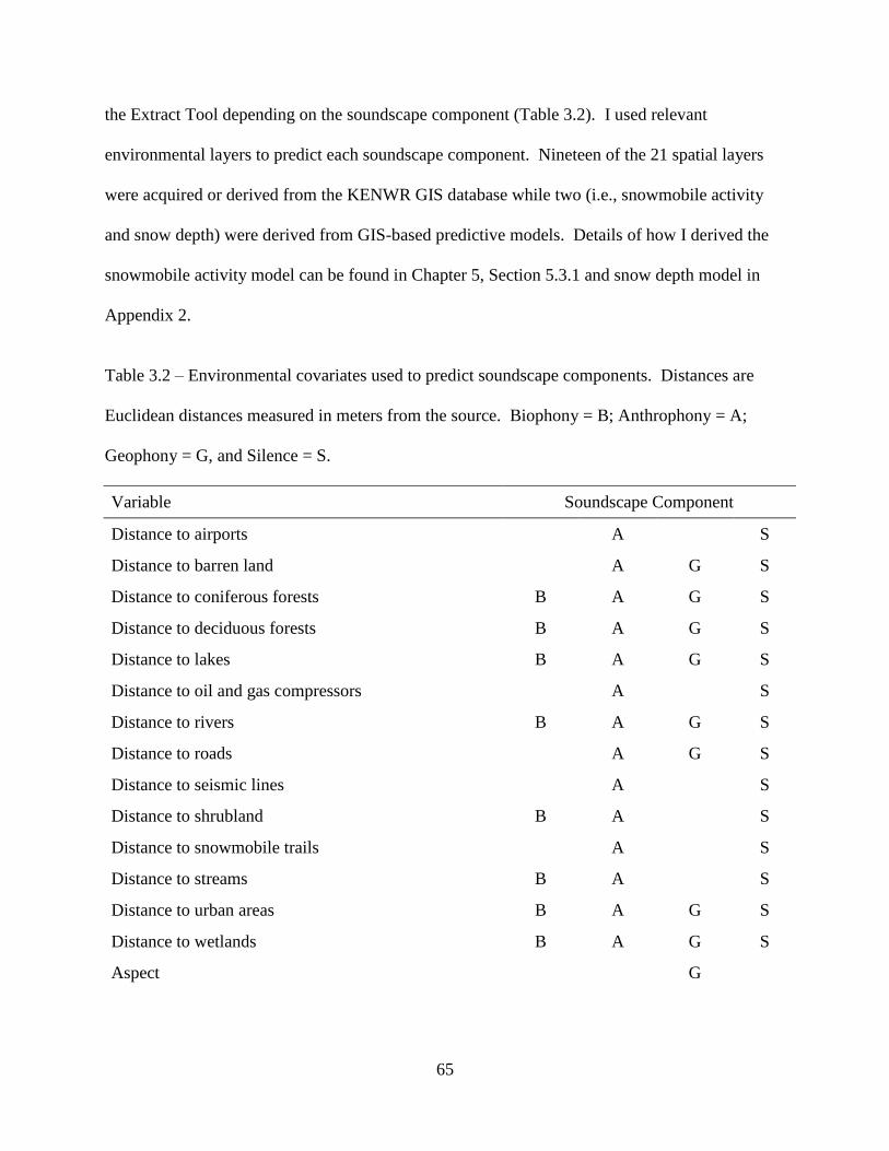
65
the Extract Tool depending on the soundscape component (Table 3.2). I used relevant
environmental layers to predict each soundscape component. Nineteen of the 21 spatial layers
were acquired or derived from the KENWR GIS database while two (i.e., snowmobile activity
and snow depth) were derived from GIS-based predictive models. Details of how I derived the
snowmobile activity model can be found in Chapter 5, Section 5.3.1 and snow depth model in
Appendix 2.
Table 3.2 – Environmental covariates used to predict soundscape components. Distances are
Euclidean distances measured in meters from the source. Biophony = B; Anthrophony = A;
Geophony = G, and Silence = S.
Variable Soundscape Component
Distance to airports
A
S
Distance to barren land
A G S
Distance to coniferous forests B A G S
Distance to deciduous forests B A G S
Distance to lakes B A G S
Distance to oil and gas compressors
A
S
Distance to rivers B A G S
Distance to roads
A G S
Distance to seismic lines
A
S
Distance to shrubland B A
S
Distance to snowmobile trails
A
S
Distance to streams B A
S
Distance to urban areas B A G S
Distance to wetlands B A G S
Aspect
G
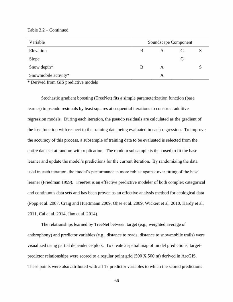
66
Table 3.2 – Continued
Variable Soundscape Component
Elevation B A G S
Slope
G
Snow depth* B A
S
Snowmobile activity*
A
* Derived from GIS predictive models
Stochastic gradient boosting (TreeNet) fits a simple parameterization function (base
learner) to pseudo residuals by least squares at sequential iterations to construct additive
regression models. During each iteration, the pseudo residuals are calculated as the gradient of
the loss function with respect to the training data being evaluated in each regression. To improve
the accuracy of this process, a subsample of training data to be evaluated is selected from the
entire data set at random with replication. The random subsample is then used to fit the base
learner and update the model’s predictions for the current iteration. By randomizing the data
used in each iteration, the model’s performance is more robust against over fitting of the base
learner (Friedman 1999). TreeNet is an effective predictive modeler of both complex categorical
and continuous data sets and has been proven as an effective analysis method for ecological data
(Popp et al. 2007, Craig and Huettmann 2009, Ohse et al. 2009, Wickert et al. 2010, Hardy et al.
2011, Cai et al. 2014, Jiao et al. 2014).
The relationships learned by TreeNet between target (e.g., weighted average of
anthrophony) and predictor variables (e.g., distance to roads, distance to snowmobile trails) were
visualized using partial dependence plots. To create a spatial map of model predictions, target-
predictor relationships were scored to a regular point grid (500 X 500 m) derived in ArcGIS.
These points were also attributed with all 17 predictor variables to which the scored predictions

67
could be applied with the appropriate target-predictor relationship. I then added the scored
prediction data to a map of KENWR in ArcGIS. For a better continuous spatial visualization, the
predicted relative index values of each soundscape component at each point in the grid were then
interpolated between neighboring points across the extent of the study area using the Interpolate-
to-Raster and Inverse Distance Weighting (IDW) tools in ArcGIS Spatial Analyst. This yielded
a continuous raster of the predicted distribution of each soundscape component in KENWR over
winter. The accuracy of each predictive model was interpreted by calculating the normalized
root mean squared error (nRMSE).
3.4 Results
3.4.1 Composition of Soundscape Components
Out of the 59,597 sound files that I identified to specific sound sources, 65% were
recordings of silence (n = 38,554). Geophonic sound events were the second most prevalent
record (19%; n = 11,587), followed by anthrophonic sounds (15%, n = 8,742) and an assortment
of biophonic sounds (1%; n = 714; Fig 3.3).

68
Figure 3.3 – Proportion of sound recordings of soundscape components.
Vocalizations made by corvids made up 42% of biophony sound records (n = 300), 30%
by other passerines (n = 211). The remaining 28% of biophony sound records consisted of vocal
raptors (e.g., owls (Strigiformes), bald eagles (Heliaeetus leucocephalus)), ducks (Anatidae),
woodpeckers (Picoides sp.), wolves (Canis lupus), coyotes (Canis latrans), ptarmigan (Lagopus
sp.), and red squirrels (Tamiasciurus hudsonicus; Fig 3.4).
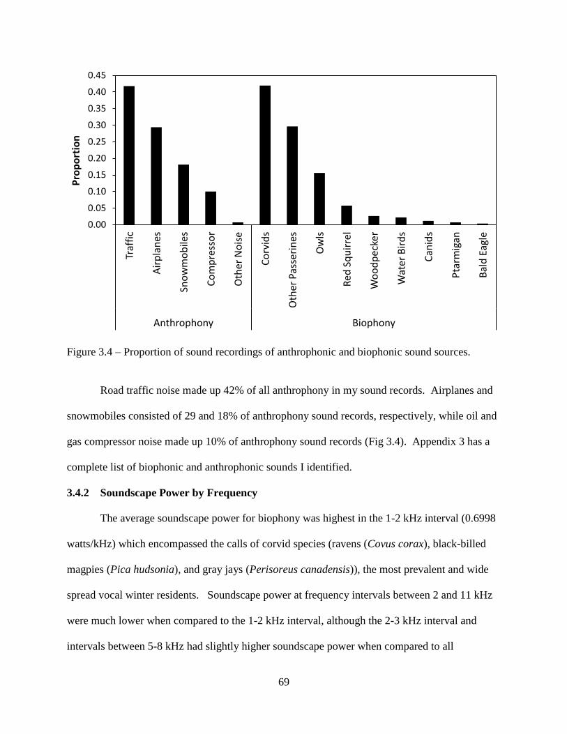
69
Figure 3.4 – Proportion of sound recordings of anthrophonic and biophonic sound sources.
Road traffic noise made up 42% of all anthrophony in my sound records. Airplanes and
snowmobiles consisted of 29 and 18% of anthrophony sound records, respectively, while oil and
gas compressor noise made up 10% of anthrophony sound records (Fig 3.4). Appendix 3 has a
complete list of biophonic and anthrophonic sounds I identified.
3.4.2 Soundscape Power by Frequency
The average soundscape power for biophony was highest in the 1-2 kHz interval (0.6998
watts/kHz) which encompassed the calls of corvid species (ravens (Covus corax), black-billed
magpies (Pica hudsonia), and gray jays (Perisoreus canadensis)), the most prevalent and wide
spread vocal winter residents. Soundscape power at frequency intervals between 2 and 11 kHz
were much lower when compared to the 1-2 kHz interval, although the 2-3 kHz interval and
intervals between 5-8 kHz had slightly higher soundscape power when compared to all
0.00
0.05
0.10
0.15
0.20
0.25
0.30
0.35
0.40
0.45
Traf
fic
Air
pla
nes
Sno
wm
ob
iles
Co
mp
ress
or
Oth
er N
ois
e
Co
rvid
s
Oth
er P
asse
rin
es
Ow
ls
Red
Sq
uir
rel
Wo
od
pec
ker
Wat
er B
ird
s
Can
ids
Pta
rmig
an
Bal
d E
agle
Anthrophony Biophony
Pro
po
rtio
n

70
remaining frequencies. These intervals consisted of other passerine species such as common
redpolls (Carduelis flammea) and black-capped chickadees (Poecile atricapillus), as well as red
squirrels (Fig 3.5).
Figure 3.5 – Mean soundscape power (watts/kHz) and 95% confidence intervals of biophony for
10 frequency intervals.
Soundscape power of anthrophony was largely within the 1-2 kHz interval where it
averaged 0.9588 watts/kHz, with a slight intrusion into the 2-3 kHz frequency interval (Fig 3.6).
There were a variety of human-made sounds (e.g., ice augers, gunshots, fireworks) but noise
from road traffic, oil and gas compressors, airplanes, and snowmobiles were predominant sound
sources (Fig 3.4). Most anthrophony power was emitted in the 1-2 kHz interval with the
exception of the revving engine of snowmobiles and propeller noise of low-flying, fixed-winged
aircraft whose soundscape power often peak at 3-4 kHz.
10-11 kHz9-10 kHz8-9 kHz7-8 kHz6-7 kHz5-6 kHz4-5 kHz3-4 kHz2-3 kHz1-2 kHz
0.8
0.7
0.6
0.5
0.4
0.3
0.2
0.1
0.0
Sound Frequency Intervals
So
un
dsca
pe
Po
we
r (w
att
s/
kH
z)
Biophony

71
Figure 3.6 – Mean soundscape power (watts/kHz) and 95% confidence intervals of anthrophony
for 10 frequency intervals.
Geophony had similar distribution and magnitude of soundscape power over frequency
intervals as anthrophony. Soundscape power for geophony was highest in the low frequency
interval of 1-2 kHz (mean = 0.9034 watts/kHz). Although there was a dramatic decrease in
soundscape power from the 1-2 kHz interval to the 2-3 kHz interval, soundscape power
gradually decreased from the intervals between 2-11 kHz (Fig 3.7). A majority of geophony was
wind, with intermittent sounds of rain and snow, flow of melting water, and cracking ice.
10-11 kHz9-10 kHz8-9 kHz7-8 kHz6-7 kHz5-6 kHz4-5 kHz3-4 kHz2-3 kHz1-2 kHz
1.0
0.8
0.6
0.4
0.2
0.0
Sound Frequency Intervals
So
un
dsca
pe
Po
we
r (w
att
s/
kH
z)
Anthrophony

72
Figure 3.7 – Mean soundscape power (watts/kHz) and 95% confidence intervals of geophony for
10 frequency intervals.
Average soundscape power of silence was highest within the 1-2 kHz interval and
gradually declined as sound frequency increased (Fig 3.8). However, soundscape power of
silence was generally much lower when compared to all other soundscape components.
Although it may seem contradictory to have soundscape power for sound files with no
recorded signal, such values are a product of the REAL method of normalizing soundscape
power. Normalization of soundscape power is done to mitigate the effects distance has on
soundscape power so that the relative energy levels between similar recordings that are different
distances from the source are similar. Since all silence sound recordings have no sound
reference and the resulting action of normalization changes the actual soundscape power value
into a relative index (based on the strength of the recordings energy), the relative soundscape
10-11 kHz9-10 kHz8-9 kHz7-8 kHz6-7 kHz5-6 kHz4-5 kHz3-4 kHz2-3 kHz1-2 kHz
0.9
0.8
0.7
0.6
0.5
0.4
0.3
0.2
0.1
0.0
Sound Frequency Intervals
So
un
dsca
pe
Po
we
r (w
att
s/
kH
z)
Geophony

73
power will automatically assign values to a silent recording. Since all silent sound files are the
same (variance = 0.0259), the normalization of these particular recordings has distinctive values
within each frequency interval (E. Kasten, pers comm.). The results of normalization therefore
enabled me to quantify silence within the frequency range I evaluated (1-11 kHz).
Figure 3.8 – Mean soundscape power (watts/kHz) and 95% confidence intervals of silence for 10
frequency intervals.
3.4.3 Temporal Variation of Soundscape Components
Daily patterns of soundscape power revealed that daylight hours (0800 – 1600 h) had the
highest amounts of sound activity. When compared across the six lowest frequencies, biophony
occurred mainly between the hours of 0800 and 1600 h (Fig 3.10).
10-11 kHz9-10 kHz8-9 kHz7-8 kHz6-7 kHz5-6 kHz4-5 kHz3-4 kHz2-3 kHz1-2 kHz
0.5
0.4
0.3
0.2
0.1
0.0
Sound Frequency Interval
So
un
dsca
pe
Po
we
r (w
att
s/
kH
z)
Silence
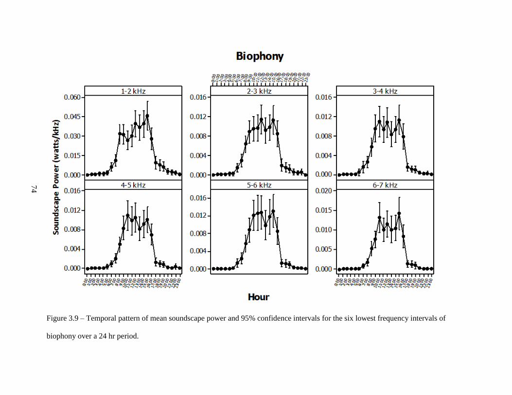
74
Figure 3.9 – Temporal pattern of mean soundscape power and 95% confidence intervals for the six lowest frequency intervals of
biophony over a 24 hr period.
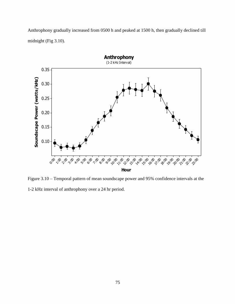
75
23:00
22:00
21:00
20:0
0
19:0
0
18:00
17:00
16:00
15:0
0
14:0
0
13:00
12:00
11:00
10:0
09:00
8:00
7:00
6:00
5:00
4:00
3:00
2:00
1:00
0:00
0.35
0.30
0.25
0.20
0.15
0.10
Hour
So
un
dsca
pe
Po
we
r (
wa
tts/
kH
z)
Anthrophony(1-2 kHz Interval)
Anthrophony gradually increased from 0500 h and peaked at 1500 h, then gradually declined till
midnight (Fig 3.10).
Figure 3.10 – Temporal pattern of mean soundscape power and 95% confidence intervals at the
1-2 kHz interval of anthrophony over a 24 hr period.
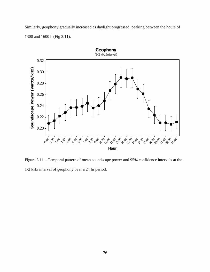
76
23:00
22:00
21:00
20:0
0
19:0
0
18:00
17:00
16:00
15:0
0
14:0
0
13:00
12:00
11:00
10:0
09:00
8:00
7:00
6:00
5:00
4:00
3:00
2:00
1:00
0:00
0.32
0.30
0.28
0.26
0.24
0.22
0.20
Hour
So
un
dsca
pe
Po
we
r (
wa
tts/
kH
z)
Geophony(1-2 kHz Interval)
Similarly, geophony gradually increased as daylight progressed, peaking between the hours of
1300 and 1600 h (Fig 3.11).
Figure 3.11 – Temporal pattern of mean soundscape power and 95% confidence intervals at the
1-2 kHz interval of geophony over a 24 hr period.

77
23:0
0
22:0
0
21:0
0
20:0
0
19:00
18:00
17:00
16:00
15:00
14:00
13:0
0
12:0
0
11:0
0
10:0
09:00
8:00
7:00
6:00
5:00
4:00
3:00
2:00
1:00
0:00
2.8
2.6
2.4
2.2
2.0
Hour
So
un
dsca
pe
Po
we
r (w
att
s/
kH
z)
Silence(Total Energy)
In contrast, periods of silence occurred during nighttime hours between 1800 to 0600 h (Fig
3.12).
Figure 3.12 – Temporal pattern of mean total soundscape power and 95% confidence intervals
for all frequency intervals of silence over a 24 hr period.
When compared, the occurrence of silence was negatively correlated to that of
anthrophony (Pearson = -0.995, p = 0.000). Additionally, despite the timing of biophony being
positively correlated with that of anthrophony (Pearson = 0.879, p = 0.000), only 18% of
biophonic sound events occurred during the same recording as anthrophony, while 8% occurred
during geophony.
The mean soundscape power of biophony (total energy) and anthrophony (1-2 kHz
interval) were positively correlated (Pearson = 0.886, p = 0.046) when soundscape power was
summarized by month (Figs 3.13 and 3.14). December and February had similar values of mean

78
soundscape power for biophony (December: n = 182, mean = 0.0559, sd = 0.3594, 95% CI
[0.045, 0.067]; February: n = 148, mean = 0.0467, sd = 0.3178, 95% CI [0.036, 0.057]) and
anthrophony (December: n = 2,466, mean = 0.2509, sd = 0.4223, 95% CI [0.240, 0.262];
February: n = 2,269, mean = 0.2556, sd = 0.4273, 95% CI [0.244, 0.268]) and were higher than
January and March (Figs. 3.13 and 3.14). April had higher soundscape power than all other
months for both biophony and anthrophony (Figs 3.13 and 3.14).
Figure 3.13 – Temporal pattern of mean total and 95% confidence intervals of soundscape power
for all frequency intervals of biophony over monthly time intervals. Letters indicate significant
differences (p < 0.05).
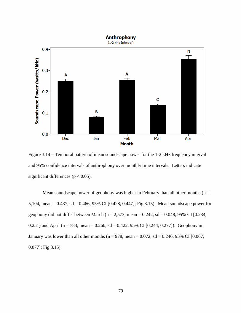
79
Figure 3.14 – Temporal pattern of mean soundscape power for the 1-2 kHz frequency interval
and 95% confidence intervals of anthrophony over monthly time intervals. Letters indicate
significant differences (p < 0.05).
Mean soundscape power of geophony was higher in February than all other months (n =
5,104, mean = 0.437, sd = 0.466, 95% CI [0.428, 0.447]; Fig 3.15). Mean soundscape power for
geophony did not differ between March (n = 2,573, mean = 0.242, sd = 0.048, 95% CI [0.234,
0.251) and April (n = 783, mean = 0.260, sd = 0.422, 95% CI [0.244, 0.277]). Geophony in
January was lower than all other months (n = 978, mean = 0.072, sd = 0.246, 95% CI [0.067,
0.077]; Fig 3.15).

80
AprMarFebJanDec
3.0
2.5
2.0
1.5
1.0
0.5
0.0
Month
So
un
dsca
pe
Po
we
r (w
att
s/
kH
z)
Silence(Total Energy)
Figure 3.15 – Temporal pattern of mean soundscape power for the 1-2 kHz frequency interval
and 95% confidence intervals of geophony over monthly time intervals. Letters indicate
significant differences (p < 0.05).
Soundscape power for silence records was higher in January (n = 15,021, mean = 2.699,
sd = 0.861, 95% CI [2.682, 2.716]) than all other months (Fig 3.16). Soundscape power was
similar for December (n = 6,789, mean = 2.174, sd = 1.343, 95% CI [2.139, 2.209]) and
February (n = 6,033, mean = 2.1505, sd = 1.344, 95% CI [2.113, 2.188]) which were
significantly lower than January and March (n = 9,030, mean = 2.544, sd = 1.081, 95% CI
[2.512, 2.565]). April had the least mean soundscape power than all other months (n = 1,681,
mean = 1.818, sd = 1.468, 95% CI [1.748, 1.889]; Fig 3.16). The occurrence of silence was
inversely correlated with that of the mean soundscape power of biophony (Pearson = -0.895, p =
0.040) and anthrophony (Pearson = -0.999, p = 0.000).
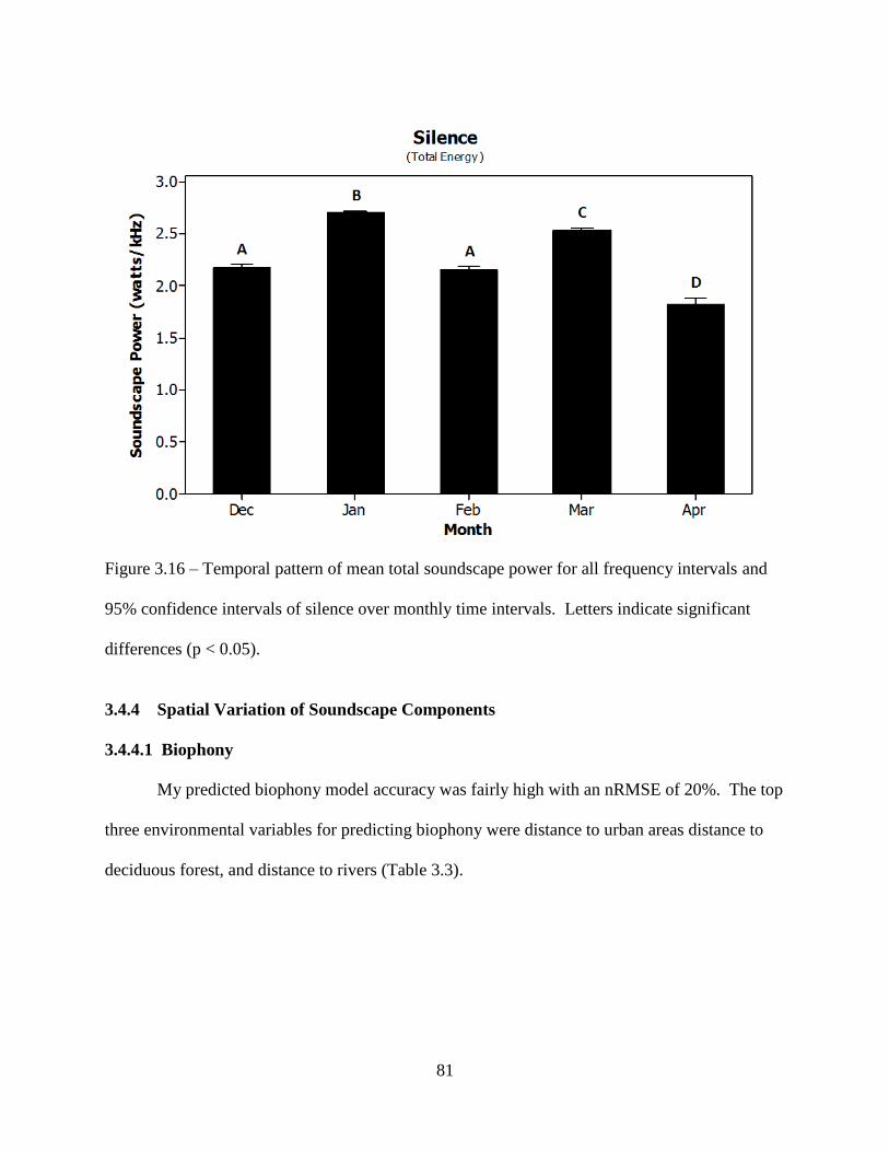
81
Figure 3.16 – Temporal pattern of mean total soundscape power for all frequency intervals and
95% confidence intervals of silence over monthly time intervals. Letters indicate significant
differences (p < 0.05).
3.4.4 Spatial Variation of Soundscape Components
3.4.4.1 Biophony
My predicted biophony model accuracy was fairly high with an nRMSE of 20%. The top
three environmental variables for predicting biophony were distance to urban areas distance to
deciduous forest, and distance to rivers (Table 3.3).

82
Table 3.3 - Variable importance of 10 environmental covariates used to predict the spatial
distribution of biophony.
Variable Score Response
Distance to urban areas 100.00 +
Distance to deciduous forest 88.42 -
Distance to rivers 81.98 -
Distance to wetlands 74.39 +
Elevation 67.38 -
Distance to Lakes 61.54 +
Snow depth* 59.11 -
Distance to streams 45.68 -
Distance to shrubland 42.25 -
Distance to conifer forest 23.05 -
* Derived from GIS predictive models
Soundscape power of biophony increased as distance to urban areas increased with much
of the soundscape power occurring ≥10 km from urban areas (Fig 3.17A). Biophony soundscape
power had an inverse relationship with distance to deciduous forest and distance to rivers.
Biophony dramatically decreased at approximately 1500 and 800 m from these landscape
features, respectively (Fig 3.17B and C).

83
Figure 3.17 – One predictor dependence for the top three environmental variables predicting
biophony: a) distance to urban areas, b) distance to deciduous forest, and c) distance to rivers.
B
A
C

84
Biophony occurred predominantly in the northern region of KENWR (Fig 3.18). There
are six major waterways in this region that were strongly spatially associated with predicted
biophony. Biophony predictions were high along the Swanson River, its tributaries, and Beaver
Creek in the northwest, Moose River and Beaver Creek in the north central, and Chickaloon
River and Big Indian Creek in the north-northeast of KENWR. South of the Sterling Highway,
biophony predictions were spatially associated with the Killey and Funny rivers. Further south,
my model predicted high biophony values along Crooked Creek and the Fox River.
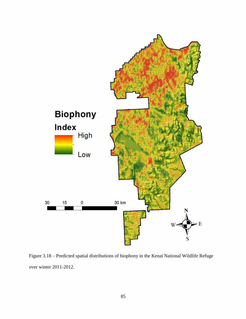
85
Figure 3.18 – Predicted spatial distributions of biophony in the Kenai National Wildlife Refuge
over winter 2011-2012.

86
3.4.4.2 Anthrophony
My anthrophony model had an nRMSE of 21% when comparing predicted soundscape
power of anthrophony to those in my sample. The top three environmental predictors of
anthrophony were distance to urban areas, distance to rivers, and distance to lakes (Table 3.4).
Table 3.4 – Variable importance of 17 environmental covariates used to predict the spatial
distribution of anthrophony.
Variable Score Response
Distance to urban areas 100.00 -
Distance to rivers 93.89 -
Distance to lakes 71.27 +
Snowmobile activity* 59.29 +
Distance to roads 56.17 -
Distance to snowmobile trails 53.09 -
Distance to oil and gas compressors 51.62 -
Elevation 36.03 -
Snow depth* 30.76 -
Distance to streams 29.40 -
Distance to wetlands 25.56 -
Distance to seismic lines 21.08 +
Distance to shrubland 20.60 +
Distance to deciduous forests 17.88 +
Distance to airports 17.43 -
Distance to coniferous forests 15.35 +
Distance to areas with no vegetation 14.08 +
* Derived from GIS predictive models
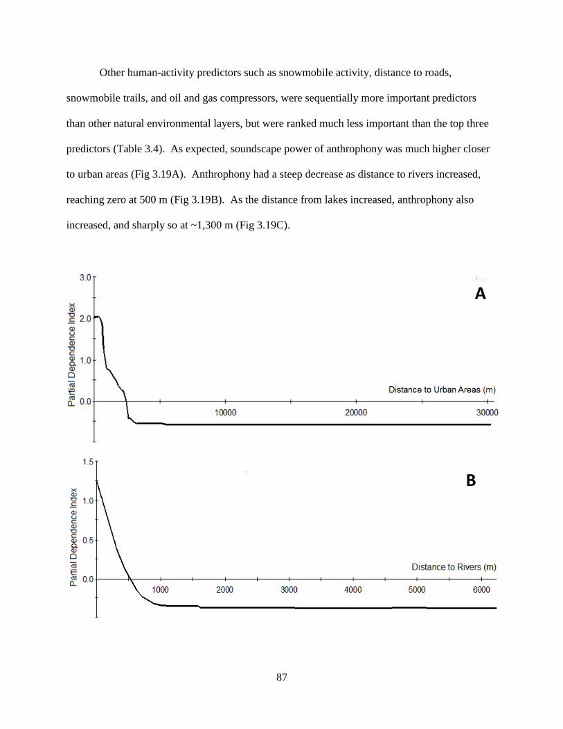
87
Other human-activity predictors such as snowmobile activity, distance to roads,
snowmobile trails, and oil and gas compressors, were sequentially more important predictors
than other natural environmental layers, but were ranked much less important than the top three
predictors (Table 3.4). As expected, soundscape power of anthrophony was much higher closer
to urban areas (Fig 3.19A). Anthrophony had a steep decrease as distance to rivers increased,
reaching zero at 500 m (Fig 3.19B). As the distance from lakes increased, anthrophony also
increased, and sharply so at ~1,300 m (Fig 3.19C).
A
B

88
Figure 3.19 – One predictor dependence for the top three environmental variables predicting
anthrophony: a) distance to urban areas, b) distance to rivers, and c) distance to lakes.
Spatially, anthrophony was strongly associated with roads and infrastructure around oil
and gas compressors in the northwest of KENWR (Fig 20). The Sterling Highway and parts of
Skilak Lake Road in the central part of KENWR had high soundscape power index values.
Relatively lower soundscape power index values were associated along rivers in the north
(Swanson River, Moose River, Mystery Creek, and Chickaloon River). In the southern part of
KENWR, Funny River, Killey River, Crooked Creek, Nikolai Creek, and Fox River were all
strongly associated with anthrophony. These landscape features are all commonly used corridors
for snowmobile-related activity (Fig 3.20).
C
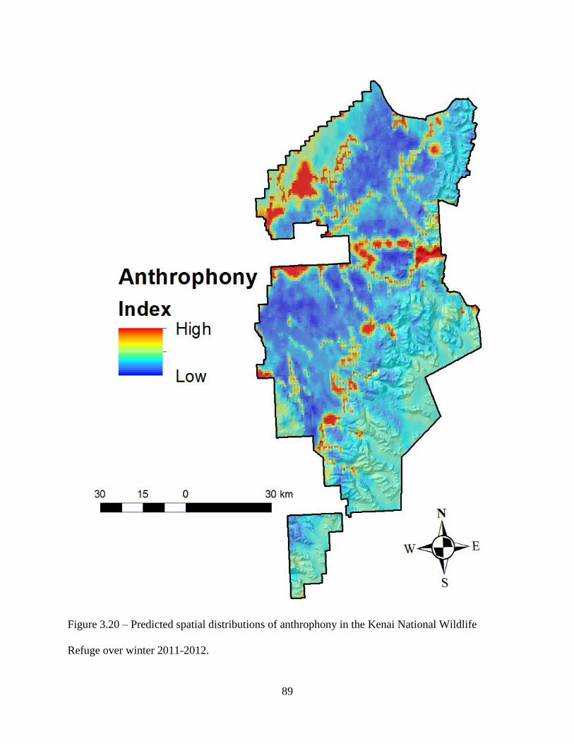
89
Figure 3.20 – Predicted spatial distributions of anthrophony in the Kenai National Wildlife
Refuge over winter 2011-2012.

90
3.4.4.3 Geophony
My geophony model was less accurate than my biophony or anthrophony models
(nRMSE = 0.28) yet still had a relative accuracy of 72%. The top three environmental variables
predicting the distribution of geophony were distance to conifer forest, elevation, and distance to
urban areas (Table 3.5).
Table 3.5 – Variable importance of 11 environmental covariates used to predict the spatial
distribution of geophony.
Variable Score Response
Distance to conifer forest 100.00 +
Elevation 84.32 +
Distance to urban areas 80.41 +
Distance to barren land 71.99 -
Distance to deciduous forest 71.35 +
Aspect 70.94 -
Distance to wetlands 67.09 +
Distance to rivers 66.68 +
Distance to roads 61.91 +
Slope 60.31 +
Distance to lakes 43.74 +
I expected conifer forests to stifle the occurrence of my most prevalently recorded
geophonic sound source, wind. Soundscape power of geophony sharply increased at 2,500 m
from conifer forests and maintained those values as distance increased (Fig 3.21A). Geophonic
power was also higher at higher elevations, increasing around 200 m above sea level (Fig 3.21B).
Distance to urban areas had a positive relationship with soundscape power of geophony with a

91
sharp increase at 10 km (Fig 3.21C). My models showed areas above treeline, such as Caribou
Hills in the southwest and the Kenai Mountains in the east, had the highest predicted values of
geophonic soundscape power (see Fig 3.22).
A
B

92
Figure 3.21 – One predictor dependence for the top three environmental variables predicting
geophony: a) distance to conifer forest, b) elevation, and c) distance to urban areas.
C
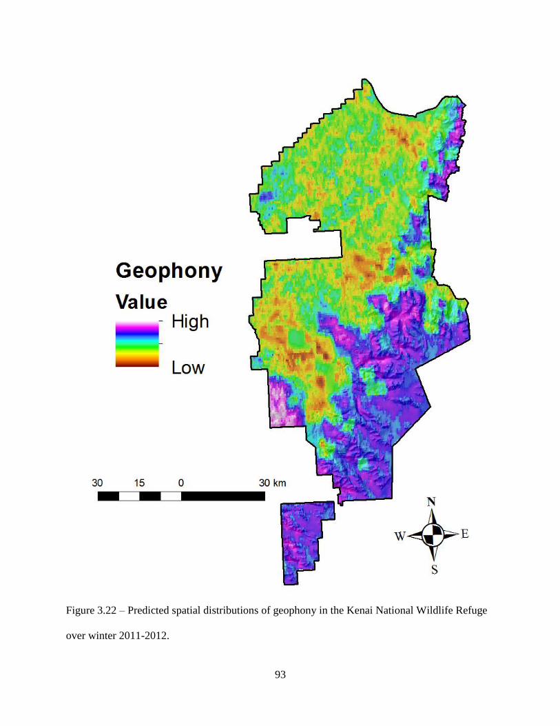
93
Figure 3.22 – Predicted spatial distributions of geophony in the Kenai National Wildlife Refuge
over winter 2011-2012.

94
3.4.4.4 Silence
The prediction accuracy of my silence model was lower than all other models (nRMSE =
0.30) although it was still 70% accurate at predicting my observed soundscape power data. The
top three predictors of silence were distance to rivers, distance to shrubland, and distance to
barren land (Table 3.6).
Table 3.6 – Variable importance of 16 environmental covariates used to predict the spatial
distribution of silence.
Variable Score Response
Distance to rivers 100.00 +
Distance to shrubland 93.62 +
Distance to barren land 82.92 -
Distance to lakes 79.42 -
Distance to snowmobile trails 79.26 -/+/-
Snow depth* 78.11 -
Distance to wetlands 74.63 -
Distance to urban areas 74.28 +
Distance to streams 73.76 +
Elevation 57.39 -
Distance to airports 54.11 +
Distance to deciduous forest 54.01 +
Distance to roads 51.90 +
Distance to oil and gas compressors 47.60 +
Distance to conifer forest 41.56 +
* Derived from GIS predictive models

95
Distance to lakes and snowmobile trails had similar rankings to distance to barren land and
therefore, shared some of the importance at predicting silence (Table 3.6). The soundscape
power of silence recordings increased with increasing distance from rivers and shrubland (Fig
3.23A and B).
B
A
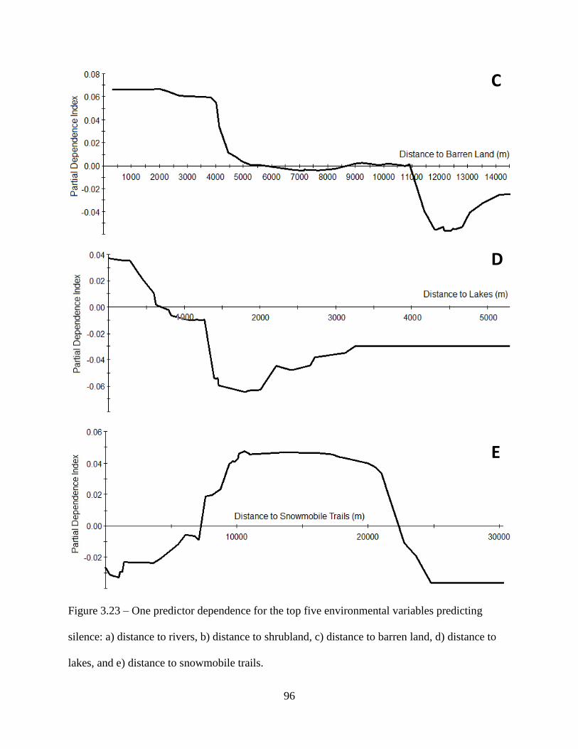
96
Figure 3.23 – One predictor dependence for the top five environmental variables predicting
silence: a) distance to rivers, b) distance to shrubland, c) distance to barren land, d) distance to
lakes, and e) distance to snowmobile trails.
D
E
C
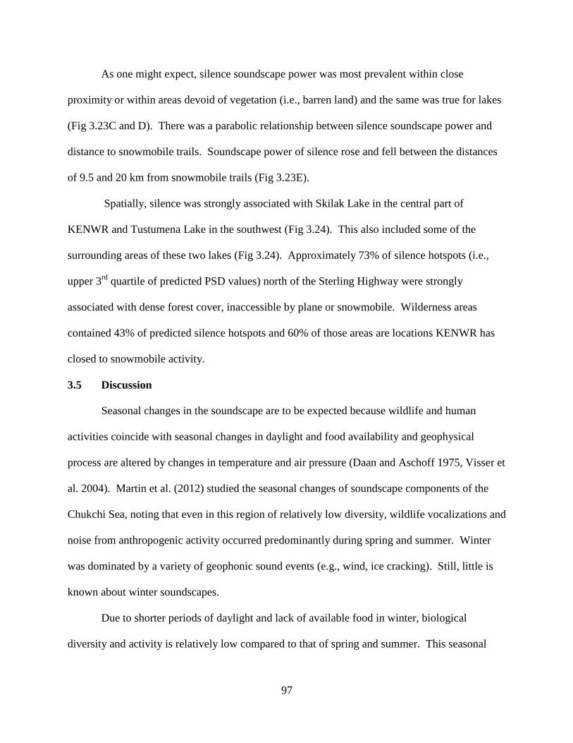
97
As one might expect, silence soundscape power was most prevalent within close
proximity or within areas devoid of vegetation (i.e., barren land) and the same was true for lakes
(Fig 3.23C and D). There was a parabolic relationship between silence soundscape power and
distance to snowmobile trails. Soundscape power of silence rose and fell between the distances
of 9.5 and 20 km from snowmobile trails (Fig 3.23E).
Spatially, silence was strongly associated with Skilak Lake in the central part of
KENWR and Tustumena Lake in the southwest (Fig 3.24). This also included some of the
surrounding areas of these two lakes (Fig 3.24). Approximately 73% of silence hotspots (i.e.,
upper 3rd
quartile of predicted PSD values) north of the Sterling Highway were strongly
associated with dense forest cover, inaccessible by plane or snowmobile. Wilderness areas
contained 43% of predicted silence hotspots and 60% of those areas are locations KENWR has
closed to snowmobile activity.
3.5 Discussion
Seasonal changes in the soundscape are to be expected because wildlife and human
activities coincide with seasonal changes in daylight and food availability and geophysical
process are altered by changes in temperature and air pressure (Daan and Aschoff 1975, Visser et
al. 2004). Martin et al. (2012) studied the seasonal changes of soundscape components of the
Chukchi Sea, noting that even in this region of relatively low diversity, wildlife vocalizations and
noise from anthropogenic activity occurred predominantly during spring and summer. Winter
was dominated by a variety of geophonic sound events (e.g., wind, ice cracking). Still, little is
known about winter soundscapes.
Due to shorter periods of daylight and lack of available food in winter, biological
diversity and activity is relatively low compared to that of spring and summer. This seasonal
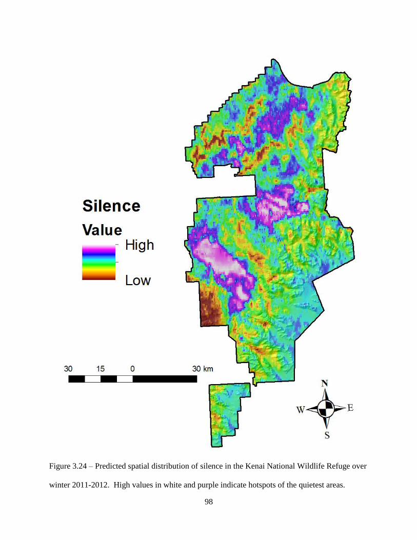
98
Figure 3.24 – Predicted spatial distribution of silence in the Kenai National Wildlife Refuge over
winter 2011-2012. High values in white and purple indicate hotspots of the quietest areas.
99
change in animal activity results in decreased biophony. This study showed that biophony had
the lowest proportion of sound records when compared to all other soundscape components.
Despite this, sound recordings effectively captured a number of vocal winter residents (Appendix
3). Of the biophony recorded, the vocalizations of corvids (ravens especially) were the most
prevalent. The soundscape power of these species occurred at low frequencies between 1-2 kHz
while other passerines (e.g., chickadees and redpolls) and squirrels occurred at higher
frequencies. I expected total soundscape power to capture the occurrence of these species for
modeling. As a result, the biophony model showed a distinct positive relationship between total
biophony soundscape power and distance further from the urban areas that border the western
edge of KENWR.
Studies have found ravens are commonly associated with human-subsidized food
resources, typically located in urban areas (Engel and Young 1992, Restani et al. 2001, Boarman
2003, Marzluff and Neatherlin 2006, Baltensberger et al. 2012) yet ravens and other passerines
in my study area were commonly recorded at sound stations far from urban areas. However, my
sample sites were biased more towards the interior of the study area rather than within urban
settings. A pilot study done of the occurrence of ravens in the Soldotna-Kenai area over January
and February 2010 revealed that raven occurrence was much higher closer to these two urban
areas around restaurants and dumpsters than in rural areas (T. Mullet, unpubl data). The ability
of ravens to utilize both natural and human-subsidized food resources on the Kenai Peninsula
over winter area is likely what enable them to be so prolific.
Biophony was also strongly associated with deciduous forests and rivers. My sample
locations were typically along forest edges. My study design and results suggest that edge
habitat close to rivers and deciduous forests are important predictors of vocal organisms. These

100
areas likely serve as travel corridors and feeding locations for wintering birds (Desrochers and
Fortin 2000).
Interestingly, I found very few sound recordings where biophony overlapped with
anthrophony and geophony, despite the similarity in their temporal occurrence and the presence
of each at respective sound stations. It is possible that vocal organisms at my sample locations
intentionally called at times when anthrophony and geophony did not occur to avoid the effects
of masking (Dooling and Popper 2007, Habib et al. 2007, Barber et al. 2010,Ortega 2012, Ortega
and Francis 2012). This behavior has been documented by Ficken et al. (1974), Brumm (2006),
and Fuller et al. (2007) on bird species that have shifted their temporal singing patterns to avoid
interference with other sounds. Considering my findings showed that anthrophony and
geophony primarily occurred at lower frequencies, wildlife who communicate at these
frequencies are probably the most affected.
Although vocalizations in winter are less likely to be territorial or play a role in
reproduction, it is known that birds, specifically, vocalize in winter to communicate with other
individuals (Ficken et al. 1978). Communication can be important for locating food during
winter when food is less abundant (Ficken 1981). Therefore, behavioral adaptations to noise are
likely to occur to increase winter survival. Certainly more research could verify this hypothesis.
The rapid increase and expansion of mechanized human activity has led to an escalation
in anthropogenic noise in the environment. Noise is expected in areas of human development
but there is evidence that anthropogenic noise is encroaching evermore into natural areas (Krause
2001, Krause and Gage 2003, Barber et al. 2010). The most common sources of anthrophony in
KENWR’s winter soundscape were those emitted by road traffic, aircraft, and motorized

101
recreation (e.g., snowmobiles), and resource extraction/development (i.e., oil and gas compressor
stations).
Road traffic and compressors in this study area were restricted to the locations in which
they were intended. However, the low frequency noise they emitted was found to extend to areas
>1 km from the source. This effect zone has been found to occur in other areas of North
America (Barber et al. 2010). In more remote locations of KENWR, noise from airplanes and
snowmobiles were the most pervasive. Over 75% of my sample locations had at least one or
more records of airplane noise and nearly 50% had one or more records of snowmobile noise.
Areas predicted by the anthrophony model indicated a strong spatial relationship to
rivers. Forests dominate most areas of KENWR where snowmobiling is allowed and frozen
rivers can serve as effective corridors into remote locations. Much of the snowmobile activity
along rivers in KENWR is speculated to be related to trapping (N. Olson, Pilot Biologist,
KENWR). Although never quantified, snowmobile activity in KENWR has noticeably increased
in the last 20 yrs and is thought to be largely related to recreational activities rather than an
increase in subsistence and trapping activity (KENWR Compatibility Determination 2007).
My models predicted the spatial extent of anthrophony and its temporal overlap with the
acoustic activity of wildlife. Anthrophony clearly has the potential to interfere with acoustic
processes or simply the quality and nature of the sonic environment (Chapter 4). Additionally,
because natural acoustic signals are less frequent in winter and remote wilderness, noise from
snowmobiles can be an alarming disturbance to unsuspecting wildlife, potentially contributing to
their physiological stress (Creel et al. 2002; Chapter 5). These results indicate that
anthropogenic noise extends well beyond the spatial footprint of infrastructure in and around
KENWR.
102
Despite the encroachment of anthrophony into remote areas of KENWR, silence
dominated most of my sound recordings and occurred at 95% of my sample sites. The
occurrence of silence in the soundscape was primarily nocturnal with few recordings during
daylight hours as a result of biological, human, or geophysical activity. However, the number of
sound recordings and the spatial distribution of silence indicate that KENWR is remarkably quiet
this time of year. An exploratory study of sound levels in KENWR during the last three weeks
of June 2004 and 2006 indicated an average A-weighted sound pressure level (dBa) from 257
sample locations was 45.1 dBa (SE = 0.68), a sound level equivalent to those recorded in
wilderness areas (EPA 1974, National Park Service 2000, Comprehensive Conservation Plan
2010).
The significance of silence has often been associated with human perception. Silence can
be meaningful in a spiritual sense as a means of respecting religious settings, meditation, and
prayer (Assagioli and Anglada 2013). Silence is also an attribute associated with respect for the
dead and is often expected during funeral ceremonies (Ehrenhaus 1988). Additionally, silence is
known to psychologically activate certain human behaviors in public buildings (Aarts and
Dijksterhuis 2003) or initiate a physiological response to induce a relaxed state of mind (Cmiel et
al. 2004). The human experience alone may be significant enough to qualify the importance of
silence as a resource to protect in some wilderness settings.
Unfortunately, the significance of silence in an ecological sense is not well understood.
Should silence have an impact on human behavior and health, it is feasible to think that such
would be the case for wildlife. Even plants have been found to be affected by sound (Retallack
1973). I know that true silence, the absence of sound, is not entirely likely as it is known that
even activity in soils create sound waves (Tornel et al. 2010, Farina 2014). Yet organisms

103
audibly perceive their sonic environment at different thresholds (Fay 1988). What one organism
or species may be able to hear is not the same as another. Therefore, silence may be perceived,
experienced, and significant at multiple levels of organization from individuals to communities.
This component of the soundscape would ultimately affect the patterns and processes of
ecological systems throughout the landscape.
The dominance of silence in my sound sampling at the frequencies I quantified provides
substantial evidence that it is just as important to the soundscape as biophony, anthrophony, and
geophony. The occurrence of silence alone could serve as a measure of wilderness quality,
levels of biodiversity, and wildlife behavior (Krause et al. 2011). With the ever encroaching
sounds of human-mechanized activity and the reduction in biodiversity around the world,
measuring silence could prove useful in evaluating conservation needs in the biosphere.
Silence could also indicate a variety of processes occurring in the landscape. Given that
my models showed a high occurrence of silence in lakes and barren lands suggests that silence is
an indicator of a lack of resources available for vocal terrestrial animals. Similarly, quiet areas
within forested areas may indicate vacancies in acoustic niches. These acoustic niches may then
be filled by migrant birds during spring, summer, and fall when resources become more
available. The discovery of silence as a significant soundscape component gives rise to many
possibilities to test its ecological significance. It is certain that quantifying silence sound records
at lower frequencies <1 kHz would prove useful to interpreting a broader frequency range of this
soundscape component.
Sound is inherent to every ecosystem (Farina 2014). Natural soundscape components
such as biophony, geophony, and silence all play roles in the dynamic processes of ecological
systems. The significance of soundscape components in winter has yet to be understood.

104
However, my results shed light on the temporal and spatial variation of winter’s soundscape
components in subarctic ecosystems. It is my intention for this study to provide an initial
understanding of sound as an important component to ecosystems in winter and to broaden our
knowledge of ecological processes in the context of sound.
105
CHAPTER 4
SNOWMOBILE NOISE EFFECTS ON
NATURALNESS AND WILDERNESS CHARACTER IN THE
KENAI NATIONAL WILDLIFE REFUGE, ALASKA
4.1 Abstract
Snowmobile recreation in the United States has been growing over the past 50 years and
has become a contentious issue in the arena of public use on federal lands. Technical
advancements in snowmobiles have enabled users to access once remote and inaccessible
wilderness areas. The Wilderness Act of 1964 has protected many of these wilderness areas
from the intrusion of snowmobiles. However, in Alaska, the Alaska National Interests Lands
Conservation Act of 1980 allows snowmobiles to be used in Congressionally-designated
Wilderness for traditional activities. The Kenai National Wildlife Refuge is one of two national
wildlife refuges in Alaska on the highway system and the only one with a significant urban
interface. Kenai National Wildlife Refuge manages the three subunits of the 525,000-ha Kenai
Wilderness (Dave Spencer, Mystery Creek, and Andrew Simons Wilderness Units) with some of
the most diverse ecological systems in the state. Accessibility to wilderness is especially high
during winter when snowmobiling is permitted. In some areas, a noticeable increase in
snowmobile activity over the years has raised concerns over the potential degradation of
wilderness character. Although snowmobile activity is known to have direct effects on wildlife
and vegetation, the noise they emit can extend to a much wider area. The detection of
snowmobile noise in wilderness areas is an indicator of degrading wilderness characteristics such
as naturalness and opportunities for solitude described in the Wilderness Act. I sought to

106
determine the spatial extent to which snowmobile noise affects Kenai Wilderness and identify
areas where natural quiet dominates. My objectives were to 1) sample the acoustic composition
of the Kenai Wilderness soundscape in winter, 2) identify the proportion to which snowmobile
noise and natural quiet contribute to the Kenai Wilderness soundscape, 3) model the spatial
distributions of snowmobile noise and natural quiet in Kenai Wilderness, and 4) quantify the
spatial extent to which snowmobile noise affects Kenai Wilderness. I recorded ambient sounds
at a total of 25 Wilderness and 37 non-Wilderness areas from December 2011 to April 2012. I
used the Remote Environmental Assessment Laboratory to calculate sound metrics which were
used to generate predictive spatial models of snowmobile noise and natural quiet using machine
learning software (TreeNet). I listened to 59,597 sound recordings to identify the proportion of
snowmobile noise and natural quiet in wilderness and non-wilderness areas. Snowmobile noise
made up 1% (n = 224) of all non-wilderness recordings (n = 32,418) but 5% (n = 1,359) of all
wilderness recordings (n = 27,179). Natural quiet made up 62% (n = 20,157) of non-wilderness
recordings and predominantly occurred at night. Natural quiet made up 70% (n = 19,111) of all
wilderness sound recordings and occurred during both day and night. Snowmobile noise
affected 32% of Kenai Wilderness where snowmobiles were permitted but did not affect
wilderness areas closed to snowmobiles. Snowmobile noise was highest closer to rivers,
wetlands, and snowmobile trails. Wilderness rivers and wetlands were accessible by
snowmobile trails along the urban interface with KENWR. Seventy-five percent of areas
predicted as hotspots where natural quiet was most prevalent were within wilderness areas. Over
half of natural quiet hotspots were within areas in which snowmobiles were prohibited. Natural
quiet was most commonly associated with areas further from wetlands, rivers, and shrublands,
and locations with snow depths <40 cm. These results provide evidence that snowmobile noise
107
extends well beyond the boundaries of infrastructure, leaving an acoustic imprint on areas where
its effects are expected to be limited. However, I also found that natural quiet shares a majority
of the acoustic environment in both wilderness and non-wilderness areas, albeit on different
temporal and spatial arrangements. Most areas of Kenai Wilderness where natural quiet
dominates still remain where snowmobiles are both permitted and restricted.
4.2 Introduction
Over the past 200 years, man’s innovations in technology and advancements in machines
have enabled mankind to significantly influence Earth’s Ecosphere (Hannah et al. 1994, Ceballos
and Ehrlich 2002). Crutzen (2006) has proposed that the evolution of the Earth has even entered
a new geological epoch called the Anthropocene. Unfortunately, this influence is not defined by
the positive, symbiotic relationship we have with the Ecosphere, but rather the negative impacts
we have forced upon the Earth. Population growth, urban sprawl, mechanization, pollution,
deforestation, desertification, species extinctions, and climate change are just some of the
consequences of our actions. One could consider these activities as the globalization of
ecological destruction. However, public laws and philosophies in human-nature interactions
have attempted to protect certain areas of the Earth from many of these destructive activities.
In the United States during the mid-19th
century and early 20th
century, philosophers like
Ralph Waldo Emerson and Henry David Thoreau brought on a new awakening of perspectives to
the separation between mankind and nature, expressing a need to become reconnected and
assigning a new ethical value to nature (Emerson 1849, Thoreau 1904). This philosophy was
reiterated by John Muir who emphasized the intrinsic values of nature and the reduction of man’s
imprint on the land (Muir 1912). Muir and President Theodore Roosevelt in the early 1900s
considered a land conservation philosophy in the U.S. which led to the formation of national

108
parks and wildlife refuges, whose purposes are to preserve the values of nature and conservation
of wildlife. However, the human land ethic to value nature for its intrinsic value was slow to
develop and the environmental philosophies of the mid-19th
century were again reemphasized in
Aldo Leopold’s A Sand County Almanac (1949) but not yet fully realized.
By the 1960s the human population in the United States had grown to more than 170
million with over 74 million motor vehicles expanding across millions of miles of paved roads.
The expansion of the road system had provided Americans motor access to many parts of the
country as well as a means to expand their imprint further from cities into more rural areas. As a
result, America’s wilderness areas were becoming increasingly at risk from anthropogenic
effects as people ironically gravitated towards recreating in nature.
In order to prevent human population growth, suburban sprawl, and mechanization from
occupying and modifying all areas within the United States, Congress passed the Wilderness Act
in 1964. This Act was an unprecedented movement towards a land ethic where nature and the
wild had intrinsic value and benefit for mankind as a non-monetary resource. The Wilderness
Act was specifically intended “to secure for the American people of present and future
generations the benefits of an enduring resource of wilderness (Section 2(a)).” Although no
additional lands were acquired by the Wilderness Act, it did designate 3.7 million hectares of
federal land as wilderness.
The Wilderness Act defines wilderness by four distinct characteristics. According to
Section 2(c), wilderness is recognized as an area “where the earth and its community of life are
untrammeled by man, where man himself is a visitor who does not remain,” 2) “of undeveloped
Federal land retaining its primeval character and influence, without permanent improvements or
human habitation,” 3) that “generally appears to have been affected primarily by the forces of

109
nature, with the imprint of man's work substantially unnoticeable,” and 4) that provides
“outstanding opportunities for solitude or a primitive and unconfined type of recreation.”
Inherent in this definition is the preservation of ecological processes that have shaped
wilderness areas in the absence of man. This state of “naturalness” provides the foundation for
wilderness areas, in that ecological processes have developed over evolutionary time and the
components of these ecosystems in their natural condition are what the Act places value on and
is intended to preserve. The human experience in wilderness is intended to contrast sharply with
that of our busy, machine-dominated society.
Alaska is unique compared to that of the contiguous United States in that it possesses
tens-of-millions of hectares of undeveloped land. In 1980, President Jimmy Carter signed into
law the Alaska National Interests Lands Conservation Act (ANILCA). This Act established
more than 42 million ha of new and expanded public land (i.e., conservation system units) into
13 national parks, 17 national wildlife refuges, several scenic rivers, recreation areas, national
monuments, and conservation areas. Over half of these conservation system units were
designated as wilderness. The purpose of ANILCA is to:
preserve for the benefit, use, education, and inspiration of present and future
generations certain lands and waters in the State of Alaska that contain nationally
significant natural, scenic, historic, archeological, geological, scientific,
wilderness, cultural, recreational, and wildlife values.
The Alaska National Interests Lands Conservation Act was a compromise by federal land
managers who needed to balance the national interests of Alaska’s unique scenic and wildlife
resources with that of Alaska’s developing economy, infrastructure, and rural way of life (Public
110
Law 96-487). Because of this, ANILCA has specific provisions for motorized access into
Alaska wilderness areas that conflict with the mandates of the Wilderness Act.
The Wilderness Act specifically states that there shall be no use of motorized equipment,
landing aircraft, use of motor vehicles, or other forms of mechanical transport except to meet
minimum requirements for the administration of the area (Section 4(c)). The provisions of
ANILCA (Sections 1110(a) and 811(b)) on the other hand, state that access on conservation units
(including designated wilderness) allows,
the use of [snowmobiles], motorboats, airplanes, and nonmotorized surface
transportation methods for traditional activities and for travel to and from villages
and homesites, [as well as], use for subsistence purposes of snowmobiles,
motorboats, and other means of surface transportation traditionally employed for
such purposes by local residents.
Although the laws assigned by ANILCA overwrite those of the Wilderness Act, it is clear that
these provisions contradict the preservation of wilderness characteristics of naturalness and
opportunities of solitude defined by the Wilderness Act.
The effects from the conflicting mandates of ANILCA and the Wilderness Act on
wilderness character are more prevalent in areas of Alaska where the human population is high
and wilderness areas are easily accessible. The Kenai National Wildlife Refuge contains over
525,000 ha of Congressionally-designated wilderness (Dave Spencer, Mystery Creek, and
Andrew Simons Wilderness Units; hereby referred to as Wilderness) with some of the
most diverse ecological systems in Alaska (Fig 4.1). The Kenai National Wildlife Refuge is
exposed to many sources of anthropogenic activities and the sounds they produce. It is one of

111
two national wildlife refuges on the highway system and the only one with a significant urban
interface.
The Sterling Highway, the only route from Homer to Anchorage, AK, bisects KENWR
making a distinct north/south separation. Along this same line the city of Soldotna borders
KENWR to the west. The northwest portion of KENWR is a site of leased oil and gas
development and is bordered closely by the communities of Kenai and Nikiski.
Additionally, Kenai Municipal Airport is a hub for small commuter aircraft flying to and from
Anchorage and Homer, whose flight path passes through KENWR’s airspace. There are also
several small airports around the peninsula that allow private pilots and commercial charter
services to explore KENWR’s wildlife and landscapes. Much of KENWR’s lands south of the
Sterling Highway are inaccessible by car. However, roads leading to boat launches are easy
access points to Skilak and Tustumena lakes (Fig 4.1).
Summer is the season with the most anthropogenic activities, with sounds generated from
an estimated one million visitors per year (KENWR Comprehensive Conservation Plan 2010).
Although out-of-state tourism greatly decreases in winter, residents from both the Kenai
Peninsula and Anchorage area come to KENWR to recreate in various activities. One of the
most wide-spread activities and sources of winter anthrophony is snowmobiling. The KENWR
currently allows snowmobiling access to over 500,000 ha (63%), over half being Wilderness (Fig
4.1).

112
Figure 4.1 – Geographical orientation of the Kenai National Wildlife Refuge, Alaska and
associated geographic features, wilderness designations (Dave Spencer, Mystery Creek, and
Andrew Simons Wilderness Units), and snowmobile restrictions.
113
To reduce the impacts snowmobiling has on wildlife and the environment, KENWR
established basic regulations to restrict the size of machines to < 101.6 cm wide, the time of use
to take place from December to April (provided there is adequate snowfall), the type of use (e.g.,
no racing or road use), and the exclusion of alpine areas (with the exception of the Caribou Hills
in the southwest; Fig 4.1). However, enforcement of these regulations is circumstantial and
judged accordingly by KENWR law enforcement making it difficult and sporadic (R. Barto,
KENWR Law Enforcement, pers comm.).
Areas north of the Sterling Highway can be accessed by snowmobile via the Swanson
River Oil Field and Mystery Creek Road. Mystery Creek Road is an unpaved road, closed to car
traffic in winter but open to snowmobilers, allowing access to 85 km of trail running north from
the Sterling Highway and southwest to northeast from Soldotna to the Chickaloon Flats on the
southern edge of Turnagain Arm (Fig 4.1). Wetlands and various small rivers also allow access
to the northeastern portion of KENWR. Snowmobile activity in the northwest can occur along
the Swanson River and surrounding wetlands accessible through the Swanson River Oil Field
and Swanson River Road (Fig 4.1).
The southern portion of KENWR can be accessed by snowmobile from several locations.
The frozen Skilak and Tustumena lakes are accessible by public boat launches off of Skilak Lake
Road and Johnson Lake Road, respectively. Both roads are secondary to the Sterling Highway
and the lakes are popular sites for trappers and recreationists. The central part of KENWR is
accessible by two horse trails (Hansen and Funny River Horse Trails) running from north to
south from Funny River Road, another secondary road from the Sterling Highway. There are
several wetlands and lakes accessible from these trails which serve primarily as trap lines and
access to a cabin in-holding. Additionally, many of the 2,900 km of seismic lines that were cut

114
through the forests of KENWR during oil and gas exploration serve as additional access points to
the interior of KENWR.
The most utilized area of KENWR by snowmobilers is the Caribou Hills (Fig 4.1).
Largely used for recreation, the Caribou Hills is the only alpine area of the KENWR open to
snowmobiling. Bisected by KENWR, state, and native land, the Caribou Hills is accessed by
multiple snowmobile trailheads that split into eight established and well maintained trails leading
straight into the hills themselves. The eastern portion of KENWR is bordered by the Kenai
Mountains where snowmobiling is restricted above treeline (Fig 4.1).
Despite the level of human activity and the noise associated with it, KENWR is relatively
quiet. Sound levels of KENWR were measured during the last three weeks of June 2004 and
2006. Ambient sound pressure levels were recorded in the absence of high wind and rain for five
minutes between 0500 and 1000 h at 5-km intervals across the entire refuge (n = 257). The data
indicated that the mean A-weighted sound pressure level was 45.1 dBa (SE = 0.68), a sound
level equivalent to whispers in a quiet library (KENWR Comprehensive Conservation Plan
2010). Although these findings suggest that KENWR is generally quiet during the mornings of
mid-summer, the low hum of an oil compressor or distant road noise can also produce the same
results. Similarly, the rushing of a river or the territorial calls of birds can produce sound
pressure levels over 70 dBa, a sound level KENWR biologists also measured along the Sterling
Highway (Brumm 2004, KENWR Comprehensive Conservation Plan 2010). The differences in
sound pressure levels and their sources can be quite dramatic and therefore inconclusive to how
“natural” an environment may be.
All things being equal, Wilderness areas in which snowmobiles are allowed are likely to
have locations dominated by natural quiet (i.e., sources of biophony and periods of silence).
115
However, the noise emitted from snowmobiles can extend to a much wider area than where they
are permitted. The detection of snowmobile noise in Wilderness would indicate the degradation
of the wilderness characteristics of naturalness and solitude defined by the Wilderness Act.
Based on this information, I sought to determine the spatial extent to which snowmobile
noise affects Kenai Wilderness and identify areas where natural quiet dominates. My objectives
were to 1) sample the acoustic composition of the Kenai Wilderness soundscape in winter, 2)
identify the proportion to which snowmobile noise and natural quiet contribute to the Kenai
Wilderness soundscape, 3) model the spatial distribution of snowmobile noise and natural quiet
in Kenai Wilderness, and 4) quantify the spatial extent to which snowmobile noise affects Kenai
Wilderness.
4.3 Methods and Materials
4.3.1 Sound Sampling and Sound Data Acquisition
I used the methods and materials outlined in Chapter 3 (Section 3.3.1) to sample
KENWR’s wilderness and non-wilderness soundscape, acquire sound data, and discriminate
soundscape components. A total of 37 sound stations were in non-Wilderness and 25 were
within Wilderness. To meet the objectives of this study, I identified sound files that were
specific recordings of snowmobile noise and natural quiet. I categorized sound recordings of all
biophony and silence as natural quiet. I excluded geophony from my definition of natural quiet
for this study because most of my geophony sound recordings were primarily of wind events and
techniques to discriminate sound files that were of varying intensities of wind, rain, and rushing
water were not practical in this case. Although I consider attributes of geophony such as light
breezes, the babbling of a creek, and light rain as components of natural quiet, they were not
included in this particular analysis.
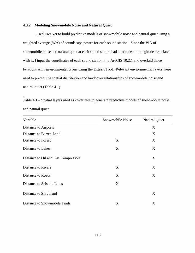
116
4.3.2 Modeling Snowmobile Noise and Natural Quiet
I used TreeNet to build predictive models of snowmobile noise and natural quiet using a
weighted average (WA) of soundscape power for each sound station. Since the WA of
snowmobile noise and natural quiet at each sound station had a latitude and longitude associated
with it, I input the coordinates of each sound station into ArcGIS 10.2.1 and overlaid those
locations with environmental layers using the Extract Tool. Relevant environmental layers were
used to predict the spatial distribution and landcover relationships of snowmobile noise and
natural quiet (Table 4.1).
.
Table 4.1 – Spatial layers used as covariates to generate predictive models of snowmobile noise
and natural quiet.
Variable Snowmobile Noise Natural Quiet
Distance to Airports X
Distance to Barren Land X
Distance to Forest X X
Distance to Lakes X X
Distance to Oil and Gas Compressors X
Distance to Rivers X X
Distance to Roads X X
Distance to Seismic Lines X
Distance to Shrubland X
Distance to Snowmobile Trails X X

117
Table 4.1 – Continued
Variable Snowmobile Noise Natural Quiet
Distance to Stream X
Distance to Urban Areas X X
Distance to Wetlands X X
Elevation X X
Snow Depth* X X
*Derived from a GIS predictive model
The relationships learned by TreeNet between target (e.g., WA of snowmobile noise) and
predictor variables (e.g., distance to roads, distance to snowmobile trails) were visualized using
partial dependence plots. To create a spatial map of model predictions, target-predictor
relationships were scored to a regular point grid (500 X 500 m) derived in ArcGIS. These points
were also attributed with all predictor variables to which the scored predictions could be applied
with the appropriate target-predictor relationship. I then added the scored prediction data to a
map of KENWR in ArcGIS. For a better continuous spatial visualization, the predicted index
values of snowmobile noise and natural quiet at each point in the grid were then interpolated
between neighboring points across the extent of the study area using the Interpolate-to-Raster
and Inverse Distance Weighting (IDW) tools in ArcGIS Spatial Analyst. This yielded a
continuous raster of the predicted distribution of snowmobile noise and natural quiet in KENWR
over winter. The accuracy of each predictive model was interpreted by calculating the
normalized root mean squared error (nRMSE).

118
4.3.3 Quantifying the Area of Snowmobile Noise and Natural Quiet in Wilderness
To quantify the amount of Wilderness affected by snowmobile noise and the proportion
of Wilderness where natural quiet dominates, I separated the values of my models’ predictions
(grid points) into quartiles and defined “hotspots” of snowmobile noise and natural quiet as
values greater than or equal to the 3rd
quartile. I then calculated the proportion of snowmobile
noise hotspots in Wilderness areas as a measure of the affected area and the proportion of natural
quiet hotspots as acoustic refugia where the Wilderness characteristics of naturalness and
solitude remain.
4.4 Results
4.4.1 Proportion of Snowmobile Noise and Natural Quiet in Wilderness and Non-
Wilderness Areas
Out of the 32,418 non-Wilderness sound recordings, anthrophony made up 20% (n =
6,591) with noise emitted from road traffic and airplanes being the most prevalent (Fig 4.2).
Snowmobile noise was identified in 1% of non-Wilderness recordings (n = 224; Fig 4.2). There
was a high proportion of natural quiet (62%; n = 20,950) in non-Wilderness areas which
predominantly occurred at night between 2100 and 0400 h, whereas anthrophony occurred
mostly during the day between the hours of 1000 and 1600 h. Geophony (primarily wind) made
up 17% (n = 5,671) of non-Wilderness recordings.
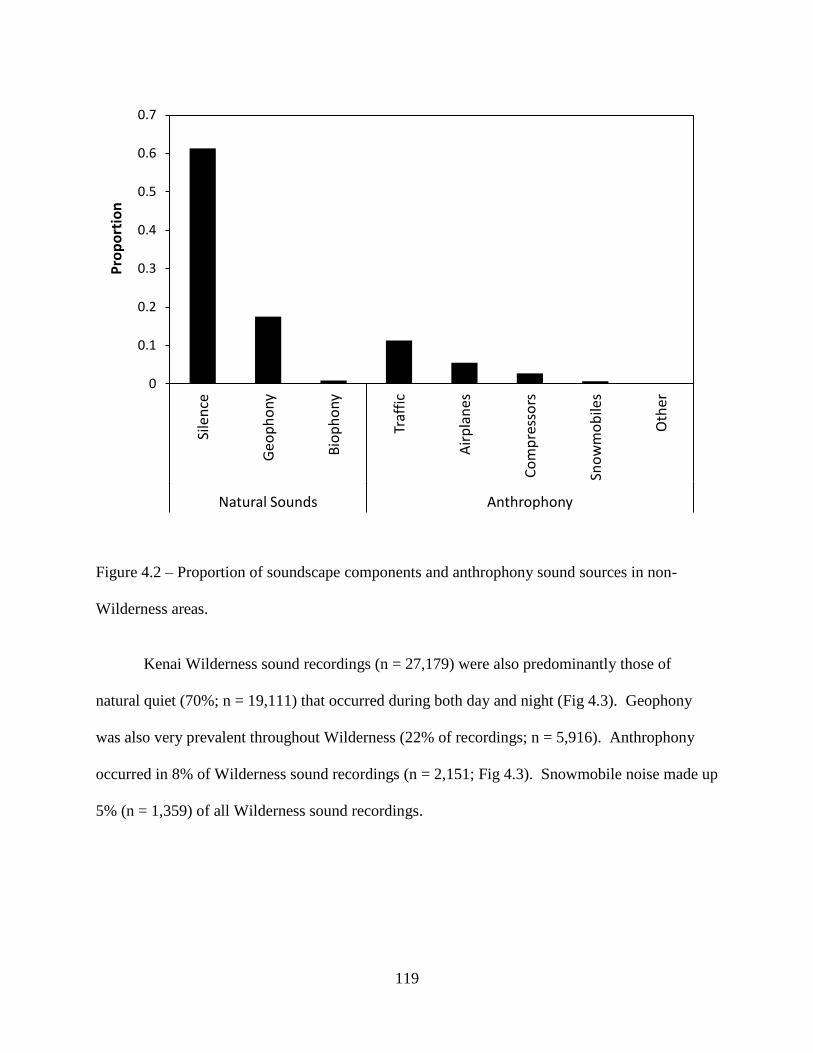
119
Figure 4.2 – Proportion of soundscape components and anthrophony sound sources in non-
Wilderness areas.
Kenai Wilderness sound recordings (n = 27,179) were also predominantly those of
natural quiet (70%; n = 19,111) that occurred during both day and night (Fig 4.3). Geophony
was also very prevalent throughout Wilderness (22% of recordings; n = 5,916). Anthrophony
occurred in 8% of Wilderness sound recordings (n = 2,151; Fig 4.3). Snowmobile noise made up
5% (n = 1,359) of all Wilderness sound recordings.
0
0.1
0.2
0.3
0.4
0.5
0.6
0.7
Sile
nce
Geo
ph
on
y
Bio
ph
on
y
Traf
fic
Air
pla
nes
Co
mp
ress
ors
Sno
wm
ob
iles
Oth
er
Natural Sounds Anthrophony
Pro
po
rtio
n

120
Figure 4.3 – Proportion of soundscape components and anthrophony sound sources in Kenai
Wilderness.
4.4.2 Model Predictions and Spatial Distribution of Snowmobile Noise and Natural Quiet
4.4.2.1 Snowmobile Noise Model and Affected Area of Wilderness
My snowmobile noise model had a relatively low error (nRMSE = 15%) when comparing
the predicted WA of soundscape power values to those recorded in my sample. Distance to
rivers, wetlands, and snowmobile trails were the top three most important environmental
predictors of snowmobile noise (Table 4.2). Predictions of snowmobile noise were highest
within 250 m of rivers, 600 m of wetlands, and 5 km from snowmobile trails (Fig 4.4).
0
0.1
0.2
0.3
0.4
0.5
0.6
0.7
0.8
Silence Geophony Biophony Snowmobiles Airplanes
Natural Sounds Anthrophony
Pro
po
rtio
n
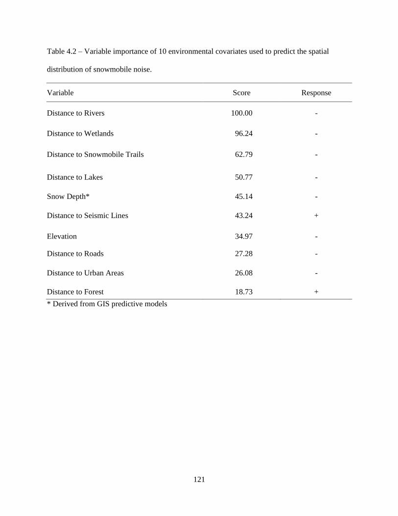
121
Table 4.2 – Variable importance of 10 environmental covariates used to predict the spatial
distribution of snowmobile noise.
Variable Score Response
Distance to Rivers 100.00 -
Distance to Wetlands 96.24 -
Distance to Snowmobile Trails 62.79 -
Distance to Lakes 50.77 -
Snow Depth* 45.14 -
Distance to Seismic Lines 43.24 +
Elevation 34.97 -
Distance to Roads 27.28 -
Distance to Urban Areas 26.08 -
Distance to Forest 18.73 +
* Derived from GIS predictive models
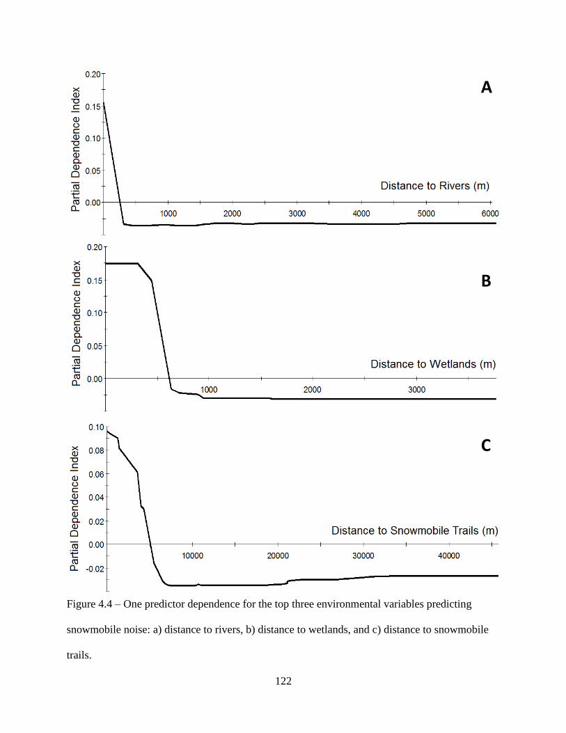
122
Figure 4.4 – One predictor dependence for the top three environmental variables predicting
snowmobile noise: a) distance to rivers, b) distance to wetlands, and c) distance to snowmobile
trails.
A
B
C
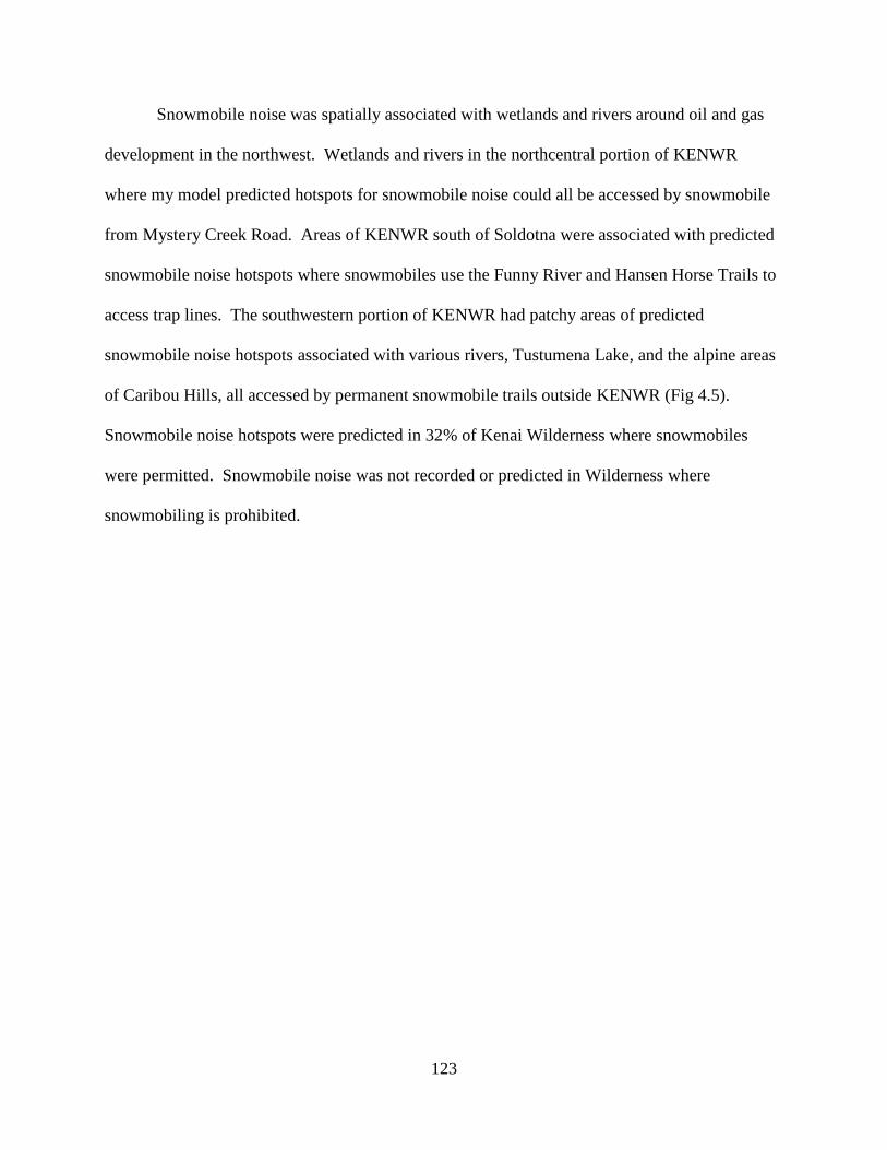
123
Snowmobile noise was spatially associated with wetlands and rivers around oil and gas
development in the northwest. Wetlands and rivers in the northcentral portion of KENWR
where my model predicted hotspots for snowmobile noise could all be accessed by snowmobile
from Mystery Creek Road. Areas of KENWR south of Soldotna were associated with predicted
snowmobile noise hotspots where snowmobiles use the Funny River and Hansen Horse Trails to
access trap lines. The southwestern portion of KENWR had patchy areas of predicted
snowmobile noise hotspots associated with various rivers, Tustumena Lake, and the alpine areas
of Caribou Hills, all accessed by permanent snowmobile trails outside KENWR (Fig 4.5).
Snowmobile noise hotspots were predicted in 32% of Kenai Wilderness where snowmobiles
were permitted. Snowmobile noise was not recorded or predicted in Wilderness where
snowmobiling is prohibited.
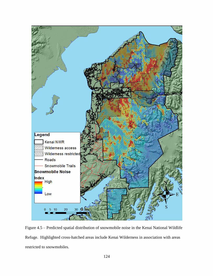
124
Figure 4.5 – Predicted spatial distribution of snowmobile noise in the Kenai National Wildlife
Refuge. Highlighted cross-hatched areas include Kenai Wilderness in association with areas
restricted to snowmobiles.

125
4.4.2.2 Natural Quiet Model and Areas of Quiet Wilderness Hotspots
My natural quiet model was less accurate than my snowmobile noise model (nRMSE =
34%) yet still had a prediction accuracy of 66% and was more accurate than if natural quiet were
randomly predicted. Distance to wetlands, rivers, shrubland, and snow depth were the top four
important predictors of natural quiet areas (Table 4.3). Natural quiet occurred most often in
areas >1.5 km from wetlands, >700 m from rivers, >2 km from shrubland, and in areas where
snow depth was <38 cm (Fig 4.6).
Table 4.3 – Variable importance of 14 environmental covariates used to predict the spatial
distribution of natural quiet.
Variable Score Response
Distance to Wetlands 100.00 +
Distance to Rivers 95.93 +
Distance to Shrubland 87.70 +
Snow Depth* 83.18 -
Distance to Barren Land 76.57 -
Distance to Urban Areas 76.50 +
Distance to Snowmobile Trails 70.01 +
Distance to Lakes 68.22 -
Distance to Streams 67.76 +
Distance to Forest 57.77 -
Elevation 54.60 +
Distance to Airports 51.87 +
Distance to Roads 47.70 +
Distance to Oil and Gas Compressors 44.85 +
* Derived from GIS predictive model

126
A
B
C
127
Figure 4.6 – One predictor dependence for the top four environmental variables predicting
natural quiet: a) distance to wetlands, b) distance to rivers, c) distance to shrubland, and d) snow
depth.
Seventy-five percent of areas my model predicted as hotspots of natural quiet were within
Kenai Wilderness and 56% of those natural quiet Wilderness areas were areas where
snowmobiling is prohibited. North of the Sterling Highway, my model predicted hotspots of
natural quiet in areas where snowmobiles were prohibited south of Swan Lake Road as well as in
small patches south of Mystery Creek Pipeline in non-Wilderness and unrestricted areas. The
snowmobile restricted region of Skilak Lake Recreation Area, south of Sterling Highway, was
also predicted as a natural quiet hotspot, as well as, a wooded region to the southwest of Skilak
Lake. Larger areas of predicted natural quiet hotspots were located on Tustumena Lake, a
heavily wooded area of mixed conifer forest to the lake’s southeast shore, and the Harding Ice
Field in the south and southeast of KENWR (Fig 4.7).
4.5 Discussion
Since the Wilderness Act was passed in 1964 the area of Wilderness in the United States
has grown from 3,600,000 ha at its inception to 42,900,000 ha today. The Alaska National
Interest Lands Conservation Act is a monument to the preservation of some of the most beautiful
D

128
Figure 4.7 – Predicted spatial distribution of natural quiet (i.e., biophony and periods of silence)
in the Kenai National Wildlife Refuge. Highlighted cross-hatched areas include Kenai
Wilderness in association with areas restricted to snowmobiles.
129
landscapes in the United States. To attest the value Americans give to these wild and scenic
landscapes, ANILCA set aside 22,700,000 ha of Alaskan Wilderness, over half the Wilderness
administered in the entire United States.
Opposition by many Alaskans over ANILCA and the establishment of “instant
wilderness” was thought to cater to “conservation faddists” and prevent Alaskans the right to
access and develop the state’s rich natural resources (Norris 2007). However, visitors from the
lower 48 states and many who only knew of Alaska’s wild majesty by word of mouth and media
thought of the state as the icon of wilderness (Norris 1985). Through ANILCA, lawmakers
attempted to reconcile the public interest to preserve Alaska’s landscapes and the many
unresolved issues in the state over native Alaskan land claims, subsistence lifestyle, energy
development, economic growth, and transportation (Willis 1985). However, ANILCA assigned
provisions to access and use of Wilderness that deviate from the original intentions of the
Wilderness Act, specifically the use of motorized vehicles for subsistence (Section 811 (b)) and
other traditional activities (Section 1110(a)). This conflicting mandate has raised issues over the
ever-growing rate of human activity in Wilderness areas (Nickas 1999).
Public lands in Alaska on the highway system, like Denali National Park and Preserve
(DENPP) and KENWR, are popular places for both in-state and out-of- state visitors.
Throughout summer, most of the Wilderness areas in these two federal land units are
inaccessible and motorized access is restricted to aircraft. However, in winter, Wilderness areas
are often accessible and readily used by snowmobiles. This activity, whether it is for subsistence
or recreation, traditionally employed or not, has remained protected under Sections 811 (b) and
1110(a) of ANILCA. The Act itself leaves the wording “traditional activities” ambiguous so the

130
interpretation of this provision by federal land managers and snowmobile users often differs, or
simply remains undefined.
With the seemingly unprecedented growth and popularity of snowmobile activity,
managers at DENPP were concerned about the effect snowmobile activity was having on
Wilderness character in the former Mount McKinley National Park (an area designated as
Wilderness by ANILCA; Denali National Park and Preserve 2000). In order to protect
Wilderness values like natural sounds and solitude and the health of plants and wildlife in the old
park from the effects of snowmobiles, DENPP defined “traditional activities” in Section 1110(a)
of ANILCA to mean any activity involving consumptive use of one or more natural resources,
such as hunting, trapping, fishing, berry picking, or similar activity and that the recreational use
of snowmobiles was not a traditional activity (CFR 36 Section 13.950). This definition
prohibited snowmobile activity in the old park of DENPP. Public feedback on DENPP’s
definition and prohibition of snowmobiling was overwhelmingly positive with 96% of all public
comments supporting the decision (Tranel 2001). However, the decision was not faced without
opposition and snowmobile associations sued the Department of Interior, standing on the rights
of ANILCA, only to drop the lawsuit a few years later. Currently, the old park remains closed to
snowmobiling.
The actions of DENPP in defining “traditional activities” of motorized transport to
protect Wilderness values opens the possibility for other federal land managers to do the same
where they see snowmobiles as a threat to Wilderness character or as an incompatible activity
with their mission. The geographical location of Kenai National Wildlife Refuge makes it a
popular and accessible location for snowmobile-related recreation. The same values of natural
sounds and solitude that were being degraded in DENPP are now of concern in KENWR (A.

131
Loranger, KENWR Manager, pers comm.). Regardless of snowmobile restrictions, the results of
my study give evidence that snowmobile noise affects a large area of Kenai Wilderness. One in
20 sound recordings in Wilderness areas were of snowmobiles and over 30% of Wilderness areas
open to snowmobiles were affected by the noise they emit. This evidence indicates that the
effects of snowmobile activity on Wilderness character extend to a much larger area than the
trammeling effects of snowmobile tracks.
I do not suggest here that recreational snowmobiling devalues an individual’s perception
of Wilderness. Rather, snowmobiling in Wilderness areas can enhance the user’s appreciation
for Wilderness, albeit a different form than what the author of the Wilderness Act, Howard
Zahniser, had envisioned in the mid twentieth century. Unfortunately, this kind of activity in
Wilderness comes at a cost to the naturalness of its character. “Traditional activities” remains
undefined by KENWR and debate over its definition to restrict snowmobile use in Wilderness,
should the KENWR manager choose to address it, will certainly be met with opposition from
snowmobile users.
In light of these findings, I found that snowmobile noise did not extend beyond the
confines of where they are permitted. Additionally, a majority of natural quiet occurred in Kenai
Wilderness, confirming that natural sounds still remain where they are expected. Interestingly
though, my model showed that over half of natural quiet hotspots were in areas where
snowmobiles were prohibted. Also, in areas inaccessible but unrestricted to snowmobiling, such
as heavily wooded areas and the interior of Tustumena Lake, were also predicted as natural quiet
hotspots. These findings indicate that 1) snowmobile restrictions preserve those Wilderness
characteristics of naturalness and solitude and 2) inaccessible areas of Kenai Wilderness where
snowmobiles are not restricted are locations of natural quiet refugia.

132
Soundscape conservation has become a growing focus in public lands in the U.S. (Pilcher
et al. 2009, Miller 2008), as well as in endangered ecosystems around the world (Monacchi
2013, Dumyahn and Pijanowski 2011, Irvine et al. 2009). The U.S. National Park Service (NPS)
has specifically identified natural soundscapes as a resource and under mandates of various
Congressional acts and policies such as the Organic Act of 1916, National Parks Air Tour
Management Act of 2000, NPS Management Policies of 2006, NPS Soundscape Management
Policy, NPS Cultural Soundscape Management Policy, and NPS Director’s Order #47
(Soundscape Preservation and Noise Management), national parks must manage natural
soundscapes as a resource for human benefits. Although the National Wildlife Refuge System
lacks these mandates to specifically manage for soundscapes, studies have shown that natural
quiet has psychological benefits to humans and influences human perceptions and values of
wilderness (Mace et al. 2004, Mace et al. 1999). Ecologically, natural sounds also play a
significant role in natural processes (Retallack 1973, Popper and Fay 1980, Hongbo et al. 2008,
Tucker et al. 2004, Farina 2014).
Under the National Wildlife Refuge System Improvement Act of 1997, the mission of the
National Wildlife Refuge System (System) is to:
administer a national network of lands and waters for the conservation,
management, and where appropriate restoration of the fish, wildlife, and plant
resources and their habitats within the United States for the benefit of present and
future generations of Americans (Sec. 4(2)) [and] each refuge shall be managed to
fulfill the mission of the System, as well as the specific purposes for which that
refuge was established (Sec. 5(3)(A)).
133
Under Title III, Sec. 301(4) (B) (i) of ANILCA, the purpose of the Kenai National Wildlife
Refuge is to conserve fish and wildlife populations and habitats in their natural diversity. It is
conceivable to consider natural quiet as a component of these habitats, as well as the diversity of
natural sounds in which they are a part.
The high proportion of natural quiet in Kenai Wilderness attests to its significance. Yet,
the character of naturalness and solitude that natural quiet helps define is isolated to areas where
snowmobiles do not typically occur or are restricted. Whether KENWR’s resource managers
choose to define “traditional activities” or identify natural quiet as a resource to manage in order
to fulfill its purpose, these results provide information that can be used and critically considered
in any management decisions they choose to make concerning snowmobiles, natural quiet, and
Wilderness.

134

135
CHAPTER 5
SPATIAL AND PHYSIOLOGICAL RESPONSES OF
MOOSE TO SNOWMOBILE ACTIVITY AND NOISE
5.1 Abstract
Snowmobiling is a popular winter activity in North America that provides a number of
human-related benefits. Over the past 20 years, the conflicts between snowmobile activity and
its effects on wildlife have been a growing concern. The combination of high-speed, rapid
maneuverability and loud noise makes snowmobiling a conspicuous and alarming stimulus in the
landscape. Wildlife are known to respond to snowmobile activity with predator-avoidance
behavior. This has resulted in increased stress levels and displacement from preferred habitats.
Moose (Alces alces) is a keystone species in KENWR that influences many ecological processes.
Not only is KENWR mandated to preserve a healthy moose population but is also required to
provide access to snowmobiling. The objectives of my study were to determine how
snowmobile activity and moose activity were spatially distributed across KENWR and whether
moose exhibited a physiological response to snowmobile traffic and noise with elevated stress
hormone levels. I quantified moose and snowmobile activity by developing an index of moose
and snowmobile tracks by overlaying a grid of 40 cells onto aerial photographs taken during
March 2011 and 2012 and tallying the number of cells where tracks were present. I created
spatially explicit predictive models of moose and snowmobile activity using the machine
learning software TreeNet and interpolated those predictions to the entire Refuge in ArcGIS. I
calculated the percent area of predicted high ( ≥17 cells with tracks) and medium moose activity
(8-16 cells with tracks) that overlapped with predicted high snowmobile activity (≥17 cells with
136
tracks) to determine whether moose were active in areas of snowmobile activity or whether
moose were selecting areas of KENWR where snowmobiles did not occur. I quantified
snowmobile traffic along trails used by snowmobilers using traffic counters. I quantified
snowmobile noise by recording the ambient sonic conditions at 62 locations across KENWR for
1 min every 30 min during the winter of 2011 and 2012 and by calculating the power spectral
density (PSD) within spectrograms using the Remote Environmental Assessment Laboratory
sound library. I identified 1,583 sound events of snowmobiles whose PSD values were primarily
within the 1-2 kHz range. I created a spatially explicit predictive model of snowmobile noise
using those PSD values in TreeNet and interpolated predictions to KENWR in ArcGIS. I
determined moose physiological response to snowmobile traffic and noise by testing their
relationship to moose glucocorticoid (GC) levels obtained from feces collected over the winters
of 2010-2011 and 2011-2012. Only 13.71% of high moose activity and 6.80% of high and
medium moose activity overlapped with high snowmobile activity. Burn areas ≤20 yrs old, snow
depths <60 cm, and areas of low snowmobile activity were the top three most important
predictors of moose activity. Snowmobile activity was strongly associated with roads, high
elevations, distance from seismic lines, and within 1 km and further than 6 km of willow stands.
Moose fecal GC levels were not significantly different (p = 0.251) when snowmobile traffic
varied from <5, 5-10, and >10 snowmobile passes within 10 days of sampling. Moose fecal GC
levels had a negative relationship with snowmobile noise (p = 0.00) but were positively related to
T3 levels (p = 0.00), percent area of willow (p = 0.02), and sex status (i.e., males, non-pregnant
females, and pregnant females; p = 0.03). My results indicate that 1) moose were spatially
avoiding areas of high snowmobile activity, 2) moose did not exhibit a significant increase in
stress response to varying intensities of snowmobile traffic, and 3) moose fecal GC was not

137
affected by snowmobile noise associated with snowmobile trails but rather, other environmental
and physiological variables.
5.2 Introduction
The continued intrusion of motorized activity and human development into areas
formally dominated by natural processes has resulted in the degradation of ecosystems around
the world (Hannah et al. 1994, Ceballos and Ehrlich 2002). These dramatic changes to the
landscape have caused a need to know where human disturbance is located and how those
locations are specifically being affected. Snowmobiling is a popular winter activity in North
America. It can have its benefits for promoting the use and appreciation of wilderness areas and
as an important utility for trappers, hunters, and others (Simpson 1987). However, snowmobile
activity also causes a variety of effects to wildlife and the environment during winter when
resources are limited and environmental conditions are severe.
Snowmobiling has enabled an increasing number of people to access formerly remote
areas in winter. The combination of high-speed, rapid maneuverability and loud noise makes
snowmobiling a conspicuous and alarming stimulus in the landscape (Mahoney et al. 2001).
Consequently, the dramatic increase in snowmobiles has increased the conflicts between
snowmobile enthusiasts and wildlife (Dustin and Schneider 2006).
Peer-reviewed literature on the subject of snowmobile impacts on wildlife is sparse but,
relative to other ecological components, is the most studied. Several studies have been
conducted in the United States, Canada, Norway, Sweden, and Svalbard, some with conflicting
results. Boyle and Samson (1985) cited that 13 of 166 articles with original data on recreational
impacts to wildlife actually addressed effects of snowmobiles on wildlife; of these articles, eight
were stated as having a negative impact, one had a positive impact, and four stated an
138
undetermined or no impact. My review of peer reviewed literature published after 1985 found
that of 19 articles specifically addressing snowmobile affects on wildlife, 16 found negative
effects while the remaining three had a positive or no effect (Table 1.1). These studies suggest
that most interactions between snowmobiles and wildlife have adverse affects.
Snowmobile disturbance, which I define as an interruption, interference, or change in an
animal’s natural behavior or physiological state caused by the presence of, or noise from,
snowmobile activity, can be perceived by wildlife as a form of predation risk (Tyler 1991,
Mahoney et al. 2001, Frid and Dill 2002). Predation risk can elicit a decision made by prey that
compromises the rate of resource acquisition or other activities to reduce the probability of death
(Frid and Dill 2002). Throughout evolutionary time, prey have developed anti-predator responses
to generalized stimuli, such as loud noises and rapidly approaching objects. Therefore,
encountering stimuli such as snowmobiles, animal responses are likely to follow the same
behavioral responses used by prey encountering predators. These anti-predator responses may
include vigilance, fleeing, and selection of habitats without the perceived risk (Frid and Dill
2002). These behaviors are typically initiated by a physiological stress response.
Stress is defined as a significant disturbance of homeostasis caused by marked or
unpredictable environmental change (Wingfield and Raminofsky 1999, Nelson 2000). In
mammals, the perception of a stimulus as threatening, such as an approaching predator or
vehicle, activates the hypothalamo–pituitary–adrenal axis which stimulates the secretion of
adrenocorticotropic hormone from the anterior pituitary. Adrenocorticotropic hormone then
stimulates the secretion of adrenal cortex steroids such as glucocorticoids (GC) that regulate
glucose metabolism (Harder 2005). The secretion of GC alters an animal’s behavior and
physiology consistent with an emergency response (i.e., fight or flight; Wingfield et al. 1998). A
139
stimulus that is infrequent, like the intermittent noise or passing of a snowmobile, may cause an
acute rise in stress hormone levels that in turn can cause animals to react behaviorally to the
perceived threat (Cyr and Romero 2009). All of these responses can affect an animal’s health
and survival without direct predation (Frid and Dill 2002).
Moose is a keystone species in northern regions of North America and Eurasia. Moose
are significant contributors to ecosystem processes. Moose browsing alone significantly alters
vegetative growth, nutrient cycling, vegetation composition, and forest development making
them a considerable factor in ecological processes (McInnes et al. 1992, Molvar et al. 1993,
Keilland et al. 1997, Kielland and Bryant 1998, Pastor and Danell 2003). Moose have evolved
specialized responses to natural environmental disturbances but have only recently been exposed
to human-caused disturbance created by machines.
Tomeo (2000) studied the response of fecal GC levels in moose to the presence of
snowmobiles in central Alaska. She found that moose in areas with snowmobile activity had
higher fecal GC levels than moose in areas where snowmobiles were not present. Colescott and
Gillingham (1998) studied the effects of snowmobile traffic on wintering moose (Alces alces) in
Greys River Valley, Wyoming. They found that moose bedding within 300 m and feeding
within 150 m of active snowmobile trails altered their behavior in response to snowmobile
disturbance. The response was more pronounced when moose were within 150 m of active
snowmobile trails. Moose appeared to move away from snowmobile trails as the day progressed.
Although snowmobile activity did not cause moose to permanently leave their preferred habitat,
it did influence moose behavior within 300 m of snowmobile traffic and temporarily displaced
moose to less favorable habitats.

140
While observing moose flight response to mechanical transports such as snowmobiles,
Anderson et al. (1996) found that moose flight distance was >1 km when a snowmobile
approached ≤5 m. Neumann et al. (2011) found that snowmobile disturbance of moose resulted
in expanded diurnal activity ranges and spatial reorganization. Harris et al. (2014) studied the
effects of snowmobile activity on moose in southcentral Alaska. Moose in their study area
moved away from areas of high snowmobile activity. They concluded that disturbance to moose
was higher when snowmobile activity was unpredictable in time and geographical location and
longer in duration (e.g., months).
Senft et al. (1987) hypothesized that decisions made on a larger spatial scale would have
a higher impact to an animal’s fitness than at finer scales. Rettie and Messier (2000) and
Dussault et al. (2005) suggested that animals and moose in particular will select habitats based
on limiting factors such as food availability and predation. Van Ballenberghe and Ballard (1998)
found that the natural limiting factors to moose in North America were predation, food
availability, weather conditions, parasites, and disease, in that order. Dussault et al. (2005)
proposed two ways that moose can select habitats to escape the effects of these limiting factors:
1) they may avoid the effect of a limiting factor directly (e.g., avoiding areas where predator
encounters are high; Rettie and Messier 2000, Mahoney and Virgil 2003) or 2) they may select
habitats where the effect of the limiting factor is reduced (e.g., use habitats with less snow fall;
Hundertmark et al. 1990).
Dussault et al.’s (2005) study of limiting factors on moose in winter found that food
availability, snow conditions, and predation were of primary importance in the selection of
habitats at both home range and landscape scales. Because of the high energetic cost of survival
in winter, moose selected habitats with more available food resources over deep snow and risk of
141
predation. Secondarily, moose selected shelter from snow but would optimize their habitat by
selecting areas where food was abundant and shelter from snow was close. Moose avoided areas
of shallow snow where wolves were predominately present (Dussault et al. 2005).
Snowmobiles can be considered an additional limiting factor that influences moose stress
response and habitat selection. Although snowmobiles do not pose a direct threat of mortality to
moose, there is evidence that moose respond to snowmobile activity by exhibiting changes in
behavior similar to other animals exposed to a threatening disturbance (Anderson et al. 1996,
Colescott and Gillingham 1998, Neumann et al. 2011). These reactions to perceived risk can be
considered a behavioral response to reduce stress (Reeder and Kramer 2005).
The decision to move away from human disturbance and its cost to the animal’s fitness
are dependent on the quality of the disturbed habitat and that of alternative habitats (Gill et al.
2001). Areas with high snowmobile activity could create a higher cost of energy to moose due to
increased energy spent on avoidance behavior and stress reduction. If this cost of avoidance
exceeds the energy they gain by staying in a particular area, moose may be displaced to less
favorable habitats (e.g., further from willow stands; Risenhoover 1989, Renecker and Schwartz
1997). This would not only affect the health of the moose population but also alter broader
ecological processes.
Conversely, moose are commonly found feeding on the secondary growth along
roadsides and in urban areas despite the higher risk of moose-vehicle collisions (Risenhoover
1989, Rea 2003, Laurian et al. 2008). In this instance, moose are likely trading off human-
related risks for food (Wasser et al. 2011). This trade off could also be attributed to the
predictability of human activity. Although human activity in urban areas is predictable,
glucocorticoid stress hormone levels of moose in urban areas was observed by Tomeo (2000) to
142
be significantly higher when compared to rural moose populations. A possible explanation for
this stress response may be related to noise.
There have been many studies on the health affects noise has on humans, confirming that
machine-generated noise is a stressor on the human body (Westman and Walters 1981). Studies
on humans have shown that noise increases blood pressure (Zhao et al. 1991, Lang et al. 1992),
heart disease (Babisch et al. 1999, Babisch 2000, Rosenlund et al. 2001), and stress hormone
levels (Brandenberger et al. 1980), and impairs memory selectivity (Smith and Broadbent 1992)
and cognitive performance (Clark and Sörqvist 2012). According to Westman and Walters
(1981), the primary role of hearing is to alert and warn. For this reason, sound evokes emotions
and actions that are directly linked to the inner ear’s connection with the “fight or flight”
mechanism of the autonomic nervous system which ultimately controls the stress response. Over
time, the auditory system of animals has evolved ways to process frequencies and intensities to
ensure survival in the sonic environments of nature. However, the recent onset of mechanical
noise in the environment has not enabled human ears sufficient time to adapt to its effects, let
alone wildlife (Westman and Walters 1981).
The meaning of a sound and its association with known or novel stimuli is important to
an animal’s reaction. A sound that is related to something threatening will have a more
significant impact on an animal’s behavior and physiology than a sound that is not. This
perception is dependent on the cognitive state of the individual and can therefore vary within a
population (Westman and Walters 1981). Differential response of an animal to noise may also
be based on its frequency and predictability (Glass et al. 1969). For example, noise from a free-
ranging snowmobile may be less predictable than the noise emitted from road traffic and more

143
threatening than the noise associated with an airplane. Therefore, an animal’s response to
snowmobile noise may be more pronounced than that of other man-made noises.
Moose have excellent hearing because of the size of the reflective surface of the outer ear
(60 times larger than the human ear). Moose also have better stereophony as a result of the
distance between the ears (twice the distance than that of humans). Additionally, because the
ears can move independently, the thresholds for calls or programmed noises may be extremely
low (Bubenik 1997). For example, moose have been known to communicate at distances of over
>1 km, using call frequencies below the threshold of human hearing (Bubenik unpubl.). It is
possible then that moose are more sensitive to low-frequency mechanical noise than humans.
The effect snowmobile noise has on wildlife has only marginally been addressed (Wanek 1971,
Dorrance et al. 1975, Moen et al. 1982). The effect of snowmobile noise on moose has not been
considered until now.
Although there is likely variability of moose response to snowmobile activity at a local
level which could be detected by measuring their stress response, moose distributions based on
habitat selection has significant effects on their overall fitness and therefore should be detected at
larger spatial scales (i.e., landscape level; Senft et al. 1987). The objectives of my study were to
determine how snowmobile activity and moose activity were spatially distributed across
KENWR and whether moose exhibited a physiological response to snowmobile traffic and noise
with elevated stress hormone levels.

144
5.3 Methods and Materials
5.3.1 Determining the Spatial Response of Moose to Snowmobile Activity
5.3.1.1 Aerial Surveys and Quantifying Moose and Snowmobile Activity
Areas of snowmobile and moose activity in KENWR were identified by creating a spatial
index of snowmobile and moose tracks from aerial photographs. Aerial photographs were taken
with a NikonTM
D700 camera, a professional grade, full-frame, digital single-lens reflex camera
with a 36 x 23.9 mm, 12.1 megapixel sensor. The D700 has a built-in, Multi-CAM 3500FX
autofocus sensor module featuring 51 AF points with 3D focus tracking. The D700 also
possesses an electronic rangefinder function, automatic correction of lateral chromatic aberration
for JPEGs, ISO sensitivity from 200 to 6400, and a GPS interface for direct “geotagging”. The
extent of each photographic frame was 300 X 210 m (0.063 km2).
Aerial surveys were conducted along seven flight transects approximately 100 km in
length that were flown in a north to south direction across KENWR. Transects were flown in a
Cessna 185 at an average above ground distance of 834 m at an average rate of 132 km/h.
Survey flights were conducted on 28 March 2011 and 29 March 2012. Snow depths within the
survey area in March 2011 ranged between 20 and 69 cm. Snow depths in March 2012 ranged
between 33 and 112 cm.
Aerial photographs (JPEGs) were input into ArcMap 10 and a grid of 8 X 5 cells were
overlaid onto each photograph. The presence or absence of snowmobile tracks and moose tracks
was determined for each grid cell and the number of presences was tallied for the entire
photograph. This provided a relative index of snowmobile and moose tracks for each 300 X 210
m photograph. Cells with dense tree cover were also tallied to account for non-detection.
145
5.3.1.2 Building Spatially Explicit Models of Moose and Snowmobile Activity
I defined a site of moose or snowmobile activity as any photograph with one or more
cells with a moose or snowmobile track, respectively. The total number of cells with moose
and/or snowmobile tracks in each georeferenced photograph was overlaid with associated
environmental layers using the Extract Tool in ArcGIS 10.2.1. I then input a spreadsheet of
these data into TreeNet to build my predictive models.
The relationships learned by TreeNet between the number of cells with
moose/snowmobile tracks and predictor variables (e.g., distance to roads, distance to
snowmobile trails, etc.) were calculated in TreeNet and visualized using partial dependence
plots. I included snowmobile activity as a predictor variable of moose activity to determine the
relationship between the two. If snowmobile activity was a strong predictor of moose activity I
accepted that snowmobile activity had some effect on moose activity and I determined whether
this was a positive or negative relationship by visualizing the partial dependence plots. If
snowmobile activity was not a strong predictor of moose activity I accepted this to mean that
moose activity was not significantly influenced by that of snowmobiles and was likely
independent.
To create a spatial map of model predictions and analyze the spatial relationship between
moose and snowmobile activity, target-predictor relationships were scored to a regular point grid
(500 X 500 m) derived in ArcGIS. These points were also attributed with all environmental
predictor variables to which the scored predictions could be applied with the appropriate target-
predictor relationship. I then added the scored prediction data to a map of KENWR in ArcGIS.
For a better continuous spatial visualization, the predicted relative index values of moose and
snowmobile activity at each point in the grid were then interpolated between neighboring points
146
across the extent of the study area using the IDW tools in ArcGIS Spatial Analyst. This yielded
a continuous raster of the predicted distributions of moose and snowmobile activity in KENWR
during March. The accuracy of each predictive model was interpreted by calculating the
normalized root mean squared error (nRMSE).
5.3.1.3 Spatial Comparison of Predicted Moose and Snowmobile Activity
To compare the distribution of moose activity to that of snowmobiles I reclassified my
predictive models into classes of high, medium, and low activity. I focused primarily on areas
predicted to be high and medium activity. High activity areas were areas predicting locations
with ≥17 cells (≥45% of all cells) with moose or snowmobile tracks and medium activity areas
between 8-16 cells (20-40% of all cells). I then converted the reclassified rasters into polygon
shapefiles and calculated the percent of total area of predicted high moose activity overlapping
with high snowmobile activity and high and medium moose activity overlapping with high
snowmobile activity. This allowed me to determine the spatial association of snowmobile
activity with that of moose.
5.3.2 Determining the Physiological Response of Moose to Snowmobile Activity and Noise
5.3.2.1 Sampling Moose Pellets for Immunoassay and Hormone Analysis
The level of glucocorticoid hormone (GC) can be used as a measure of the intensity of
environmental stress (Franzmann et al. 1975). Therefore, determining the GC levels of an
animal can give insight into how a stimulus is affecting an animal’s physiological condition
which ultimately affects an animal’s ability to adapt behaviorally. Fecal analysis of GC
secretions is an effective and non-invasive alternative to the invasive measures of stress such as
blood analysis, heart rate monitoring, respiratory rate, and body temperature (Creel 1997,
Millspaugh et al. 2001, Creel et al. 2002, Wasser et al. 2011). Creel (1997) found that fecal GC

147
analysis also provides a better measure of stress levels in an individual over a longer period of
time. Fecal GC levels typically indicate the level of hormone 12 to 24 hours prior to defecation
(Millspaugh 1999). Fecal hormone analysis is often the most practical, non-invasive method for
establishing normative endocrine data and is the preferred method for examining baseline
hormone measurements in the wild (Creel 1997, Millspaugh et al. 2001, Creel et al. 2002,
Wasser et al. 2011).
Fecal samples were searched for and collected where present en route to sound recording
stations which took place every 7-10 days over the course of two winters (December 2010-April
2011 and December 2011-April 2012). Once a fecal pile was found, a GPS coordinate was taken
for that location. Ten pellets were then collected from the pile at random.
Fecal GC samples have been known to remain stable for at least two weeks following
defecation (S. Creel pers comm., Montana State University). Because I sampled during winter,
pellets remained frozen over the course of my sample period which preserved samples in the
field from rapid desiccation. Therefore, I was not overly concerned about the age of the samples
I collected and because I visited locations multiple times within a short interval, samples were
likely ≤10 days old. I stored fecal samples in a freezer at -20°C.
Several physiological factors are known to affect the levels of GC in fecal samples in
addition to environmental factors (Goyman 2012). In order to incorporate these physiological
factors, DNA for sexual identification, progesterone for pregnancy status, and triiodothryronine
(T3) as a measure of nutritional stress were extracted from fecal samples.
Immunoassays were conducted by the Center for Conservation Biology, University of
Washington. All fecal samples were swabbed for DNA using foam swabs saturated in PBS
buffer to remove mucosal cells from the surface of the moose pellets, in duplicate. Two different

148
pellets of the same sample were used for each swab, and both of the swabbed pellets plus an
additional pellet were kept intact in labeled bags in case re-swabbing was necessary (R. Booth,
University of Washington).
All remaining moose pellets of each sample were homogenized, and a portion of that was
freeze-dried. All samples were freeze-dried for 24-48 hours in a Labconco Freeze-Dry system at
-50˚C, and then thoroughly homogenized into fine powder. Approximately 0.1 g was weighed
from each sample, and a pulse-vortex double extraction with 15mL 70% ethanol was performed.
Ethanol extracts were then stored at -20˚C until assay. Radioimmunoassays (RIA) were
performed on ethanol extracts at previously validated dilutions for both fecal metabolites of
cortisol and progesterone, using MP Biomedicals’ 125-I corticosterone kit, 125-I Total T3 kit &
an in-house 3-H progesterone assay, respectively. Fecal hormone levels were then reported as ng
per gram of dried feces (R. Booth, University of Washington).
DNA was extracted from each swab using a modified version of Qiagen’s DNeasy Tissue
kit in a PCR-product free lab, with negative controls included. All samples were PCRed on
duplicate extracts to determine gender using primers SE47 & SE48, and were run 3-5 times
depending on success rate. Both positive and negative controls were included in the PCR assay.
PCR products were run with capillary electrophoresis on an ABI 3100 Genetic Analyzer and data
was analyzed using SoftGenetics’ GeneMarker software. All hormone extracts were run in
duplicate in each assay, and only those with intra-assay variation (%CV) <10% were accepted,
and controls were included in each assay to track inter-assay variation (R. Booth, University of
Washington).

149
5.3.2.2 Monitoring Snowmobile Traffic
I monitored snowmobile traffic along snowmobile trails within KENWR to determine
whether moose stress response is also related to the intensity of snowmobile activity in areas
where moose and snowmobile activity overlapped and fecal pellets were collected. I used
TRAFxTM
(TRAFx Research Ltd., Canmore, Alberta, Canada) traffic counters placed beneath
the snow of snowmobile trails to count the number of snowmobile passes over the course of my
sample periods. These traffic counters detect the electromagnetic signature of passing vehicles
and have a detection radius of 5 m. Data were stored digitally to the traffic counter. I
downloaded data from the counters every two weeks and then uploaded data into TRAFx
Communicator v2 software. I calculated the intensity of snowmobile traffic within 10 days of
each moose fecal sample I collected with respect to its location as the amount of snowmobile
activity along snowmobile trails a moose could be exposed to within my sample area.
5.3.2.3 Sound Sampling, Sound Data Acquisition, and Modeling Snowmobile Noise
Methods for sound sampling and sound data acquisition are detailed in Chapter 3, Section
3.3.1. I used the same model of snowmobile noise used in Chapter 4 to determine its effects on
moose stress hormone levels. Methods to create this snowmobile noise model are outlined in
Chapter 4, Section 4.3.2.
5.3.2.4 Data Analysis of Stress, Snowmobile Traffic, and Noise
I performed a Kruskal-Wallis Test to determine whether varying amounts of snowmobile
traffic (i.e., <5, 5-10, and >10 passes within 10 days prior to sample collection) had a significant
effect on moose fecal GC levels. I determined there to be a significant effect if p-values were
less than α = 0.05.

150
The combination of the physiological condition of an animal, and the environment it is
exposed to, has varying effects on fecal GC levels (Goyman 2012). I made an a priori list of
factors that I was able to measure to incorporate into my interpretation of the stress response of
moose (Table 5.1). Dussault et al. (2005) found that food and shelter are driving forces for
moose habitat selection and winter survival. Willow is known to be an important browse species
for Alaskan moose in winter (Oldemeyer et al. 1977, Risenhoover 1989) and the presence of
forested areas for shelter from deep snow and predators within the vicinity of preferred food
resources has been documented by Hundertmark et al. (1990) and Dussault et al. (2005). The
availability of these habitats within the vicinity of the daily activities of moose is likely to affect
stress due to their tendency to increase the area in which they move with the number of feeding
bouts (Risenhoover 1986). Given this information, a lack of these resources within a moose’s
daily winter activity range (~1 km2; Risenhoover 1986) suggests an increase in energy
expenditure to find new resources resulting in decreased feeding bouts. Therefore, the area of
preferred habitat (e.g., willow) within the vicinity of a moose is likely to decrease hormone stress
and an increase area of less preferred or non-habitat would increase a hormonal stress response
(Table 5.1).
Temperature has been known to have significant physiological effects on moose and an
important variable in the interpretation of fecal hormone response to particular environmental
variables (Goyman 2012). Belovsky and Jordan (1978), Renecker and Hudson (1986), and
Lenarz et al. (2009) have found that temperatures above a certain threshold (>-5°C in winter and
>14°C in summer) have caused significant changes in moose metabolism, respiration rates,
reduced feed intake and body weight, and increased mortality as a result of heat stress. The

151
number of days in winter when moose are exposed to temperatures >-5°C would likely increase
the level of fecal GC (Table 5.1).
Corticosterone levels vary significantly between sexes and can be associated with the
increasing levels of progesterone in females during the luteal phase (Handa et al. 1994, Kejantie
2006). Higher levels of progesterone typically found in pregnant females are also known to
result in elevated corticosterone (Oettel and Mukhopadhyay 2004). Therefore, it was important
to consider how males, non-pregnant females, and pregnant females affected the results of fecal
GC analysis. Pregnancy status was interpreted by graphing the frequency distribution of
progesterone of female moose. As a result of a distinct separation in progesterone levels, I
divided females into those who were pregnant (progesterone levels >6,000 ng/g) and not
pregnant (progesterone levels <6,000 ng/g; Fig 5.1). Males were identified through DNA
analysis.
To analyze the relationship between fecal GC and snowmobile traffic and noise with
respect to additional explanatory environmental covariates (i.e., habitat variables), I created a 1
km radius buffer around the coordinate where each group of fecal pellets was collected and
calculated the percent area of habitat covariates (e.g., percent area of willow) in ArcGIS. I also
overlaid my sample points onto my snowmobile noise model (Chapter 4) and interpolated those
values around each point within a 1 km radius using the Extract Tool in ArcToolbox. Heat stress
was interpreted as the number of days within a 10 day period of sampling that a moose could
have been exposed to temperatures >-5°C.
I performed a multiple linear regression in R to determine what physiological (i.e., T3,
sex status) and environmental covariates (including snowmobile noise) had a significant effect
on moose fecal GC levels. I selected eight predictor variables to explain the variation in

152
Figure 5.1 – Distribution of female moose progesterone levels (ng/g) and the selected
segregation of pregnant females from non-pregnant females. Normal distribution curves are
presented to show the separation between groups.
fecal GC levels (Table 5.1). I used an iterative process using Akaike’s Information Criterion
(AIC) to select which covariates best fit my regression models which I calculated in R (Burnham
and Anderson 2002). I averaged all models (from a null model to a full model using all a priori
covariates) and ranked them using a corrected AIC (AICc) in R with the package ‘AICcmodavg’
(Mazerolle 2014). I then created a table of the linear regression results for the top ranked
model(s). I determined covariates to have a significant effect on moose fecal GC levels if their
p-values were less than α = 0.05.
200001200060000
0.00030
0.00025
0.00020
0.00015
0.00010
0.00005
0.00000
Progesterone
De
nsit
yNot Pregnant
Pregnant
Status
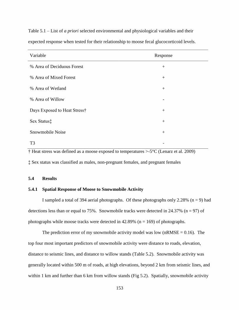
153
Table 5.1 – List of a priori selected environmental and physiological variables and their
expected response when tested for their relationship to moose fecal glucocorticoid levels.
Variable Response
% Area of Deciduous Forest +
% Area of Mixed Forest +
% Area of Wetland +
% Area of Willow -
Days Exposed to Heat Stress† +
Sex Status‡ +
Snowmobile Noise +
T3 -
† Heat stress was defined as a moose exposed to temperatures >-5°C (Lenarz et al. 2009)
‡ Sex status was classified as males, non-pregnant females, and pregnant females
5.4 Results
5.4.1 Spatial Response of Moose to Snowmobile Activity
I sampled a total of 394 aerial photographs. Of these photographs only 2.28% (n = 9) had
detections less than or equal to 75%. Snowmobile tracks were detected in 24.37% (n = 97) of
photographs while moose tracks were detected in 42.89% (n = 169) of photographs.
The prediction error of my snowmobile activity model was low (nRMSE = 0.16). The
top four most important predictors of snowmobile activity were distance to roads, elevation,
distance to seismic lines, and distance to willow stands (Table 5.2). Snowmobile activity was
generally located within 500 m of roads, at high elevations, beyond 2 km from seismic lines, and
within 1 km and further than 6 km from willow stands (Fig 5.2). Spatially, snowmobile activity
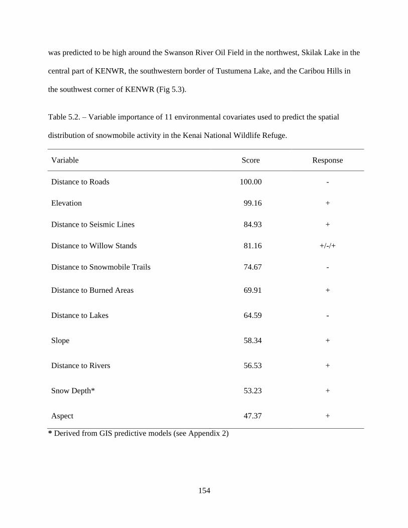
154
was predicted to be high around the Swanson River Oil Field in the northwest, Skilak Lake in the
central part of KENWR, the southwestern border of Tustumena Lake, and the Caribou Hills in
the southwest corner of KENWR (Fig 5.3).
Table 5.2. – Variable importance of 11 environmental covariates used to predict the spatial
distribution of snowmobile activity in the Kenai National Wildlife Refuge.
Variable Score Response
Distance to Roads 100.00 -
Elevation 99.16 +
Distance to Seismic Lines 84.93 +
Distance to Willow Stands 81.16 +/-/+
Distance to Snowmobile Trails 74.67 -
Distance to Burned Areas 69.91 +
Distance to Lakes 64.59 -
Slope 58.34 +
Distance to Rivers 56.53 +
Snow Depth* 53.23 +
Aspect 47.37 +
* Derived from GIS predictive models (see Appendix 2)

155
A
B
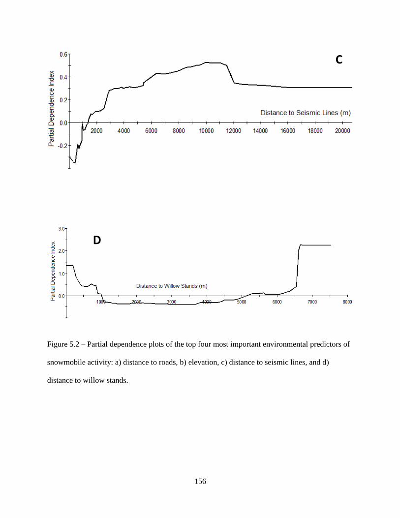
156
Figure 5.2 – Partial dependence plots of the top four most important environmental predictors of
snowmobile activity: a) distance to roads, b) elevation, c) distance to seismic lines, and d)
distance to willow stands.
D
C

157
Figure 5.3 – Predicted spatial distribution of snowmobile and moose activity in Kenai National
Wildlife Refuge in March.
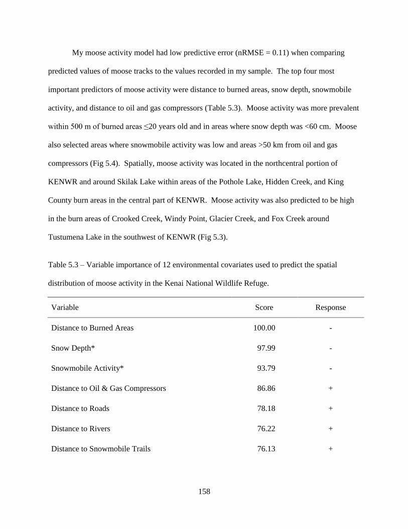
158
My moose activity model had low predictive error (nRMSE = 0.11) when comparing
predicted values of moose tracks to the values recorded in my sample. The top four most
important predictors of moose activity were distance to burned areas, snow depth, snowmobile
activity, and distance to oil and gas compressors (Table 5.3). Moose activity was more prevalent
within 500 m of burned areas ≤20 years old and in areas where snow depth was <60 cm. Moose
also selected areas where snowmobile activity was low and areas >50 km from oil and gas
compressors (Fig 5.4). Spatially, moose activity was located in the northcentral portion of
KENWR and around Skilak Lake within areas of the Pothole Lake, Hidden Creek, and King
County burn areas in the central part of KENWR. Moose activity was also predicted to be high
in the burn areas of Crooked Creek, Windy Point, Glacier Creek, and Fox Creek around
Tustumena Lake in the southwest of KENWR (Fig 5.3).
Table 5.3 – Variable importance of 12 environmental covariates used to predict the spatial
distribution of moose activity in the Kenai National Wildlife Refuge.
Variable Score Response
Distance to Burned Areas 100.00 -
Snow Depth* 97.99 -
Snowmobile Activity* 93.79 -
Distance to Oil & Gas Compressors 86.86 +
Distance to Roads 78.18 +
Distance to Rivers 76.22 +
Distance to Snowmobile Trails 76.13 +

159
Table 5.3 – Continued.
Variable Score Response
Distance to Willow Stands 75.61 +
Distance to Wetlands 74.81 +
Slope 74.70 -
Elevation 71.88 -
Aspect 70.40 -
* Derived from GIS predictive models
My models predicted there to be a 244.48 km2 area of high moose activity, 1,994.79 km
2
of high and medium moose activity combined, and 579.64 km2 area of high snowmobile activity.
Only 13.71% (33.53 km2) of predicted high moose activity areas overlapped with that of high
snowmobile activity areas and 6.80% (135.65 km2) of predicted high and medium moose activity
areas overlapped with that of high snowmobile activity (Fig 5.5). Areas of overlapping activity
were on average 3.5 km from roads and 20.6 km from snowmobile trails.
A
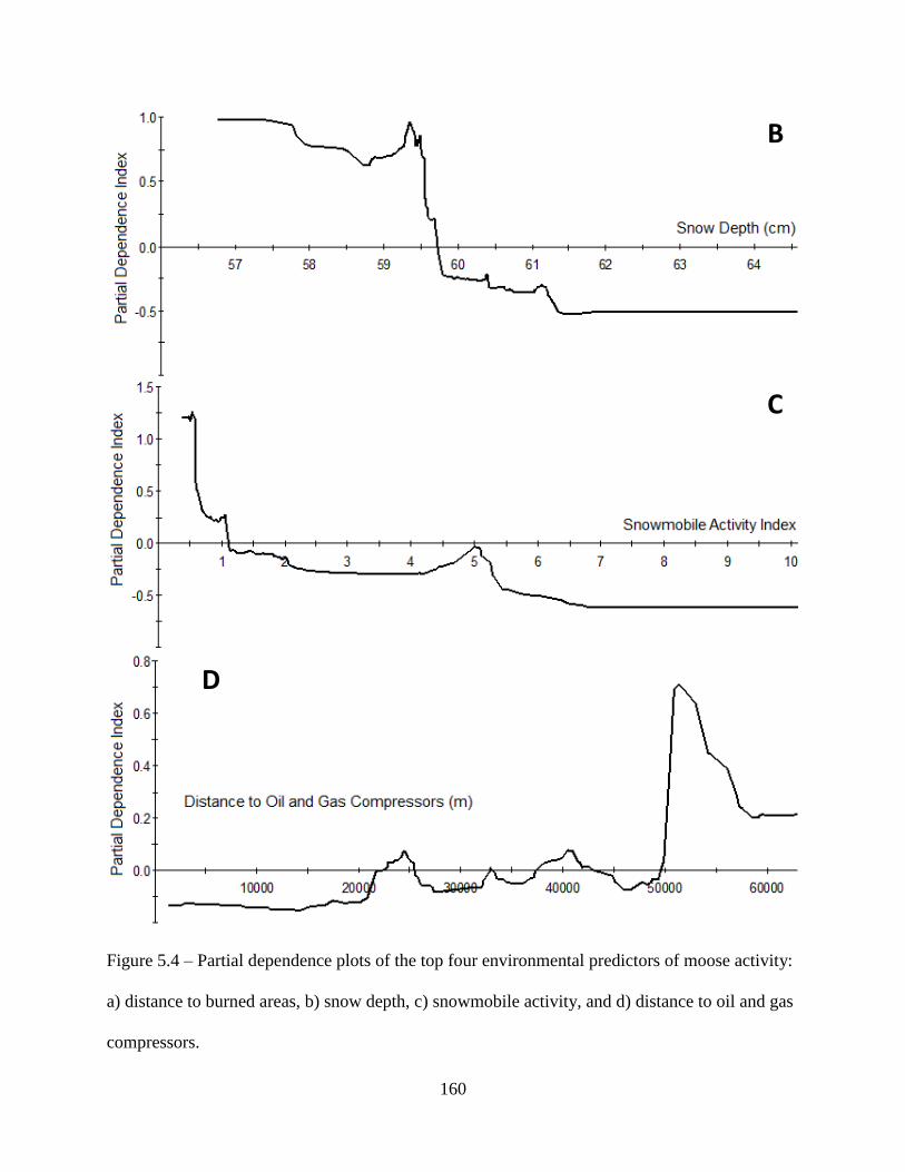
160
Figure 5.4 – Partial dependence plots of the top four environmental predictors of moose activity:
a) distance to burned areas, b) snow depth, c) snowmobile activity, and d) distance to oil and gas
compressors.
B
C
D

161
Figure 5.5 – Areas where predicted high levels of moose activity overlap with predicted high
levels of snowmobile activity (red) and areas where predicted high and medium levels of moose
activity overlap with predicted high levels of snowmobile activity (yellow).

162
5.4.2 Moose Physiological Response to Snowmobile Traffic
I collected a total of 130 moose fecal samples. Of these samples, 87% were collected on
or near a snowmobile trail. Male moose had an average fecal GC level of 163.62 ng/g (SD =
42.5; Range = 308 – 102 ng/g; n = 65). Non-pregnant females had an average fecal GC of
204.65 ng/g (SD = 56.56; Range = 324 – 119; n = 23) while pregnant females had an average
fecal GC of 192.77 ng/g (SD = 56.12; Range = 314 – 69; n = 43). As comparison, fecal GC
samples taken in the urban area of Kenai, AK, male fecal GC levels averaged 116.44 ng/g (SD =
17.38; Range = 136 – 102 ng/g; n = 3) and pregnant females averaged 248.34 ng/g (SD = 206.04;
Range = 546 – 91 ng/g; n = 7). When moose fecal GC was compared to varying intensities of
snowmobile traffic along snowmobile trails (i.e., <5, 5-10, and >10 snowmobile passes within 10
days of sampling), I found there to be no significant difference between moose fecal GC levels
and traffic intensities (p = 0.251; Fig 5.6).
5.4.3 Moose Physiological Response to Snowmobile Noise
My snowmobile noise model had a relatively low error (nRMSE = 0.15) when comparing
predicted soundscape power values to those recorded in my sample. Distance to rivers,
wetlands, and snowmobile trails were the top three most important environmental predictors of
snowmobile noise (Table 5.4). Predictions of snowmobile noise were highest within 250 m of
rivers, 600 m of wetlands, and 5 km from snowmobile trails (Fig 5.7).
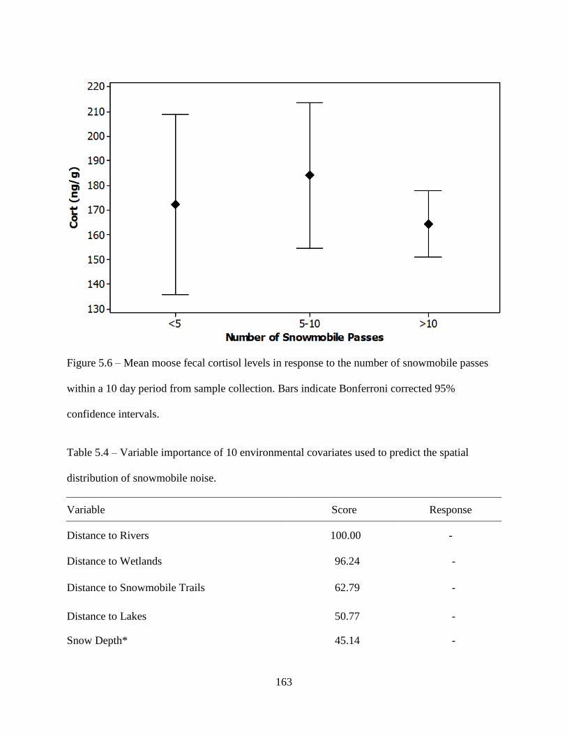
163
Figure 5.6 – Mean moose fecal cortisol levels in response to the number of snowmobile passes
within a 10 day period from sample collection. Bars indicate Bonferroni corrected 95%
confidence intervals.
Table 5.4 – Variable importance of 10 environmental covariates used to predict the spatial
distribution of snowmobile noise.
Variable Score Response
Distance to Rivers 100.00 -
Distance to Wetlands 96.24 -
Distance to Snowmobile Trails 62.79 -
Distance to Lakes 50.77 -
Snow Depth* 45.14 -

164
Table 5.4 – Continued
Variable Score Response
Distance to Seismic Lines 43.24 +
Elevation 34.97 -
Distance to Roads 27.28 -
Distance to Urban Areas 26.08 -
Distance to Forest 18.73 +
* Derived from GIS predictive models (see Appendix 2)
Snowmobile noise was spatially associated with wetlands and rivers around oil and gas
compressors in the northwest. Wetlands and rivers in the north-central portion of KENWR
where areas of high snowmobile noise were predicted were accessible by snowmobile from
Mystery Creek Road. Areas of KENWR south of Soldotna were associated with high
snowmobile noise predictions where snowmobiles use the Funny River and Hansen Horse Trails
to access trap lines. The southwestern portion of KENWR had patchy areas of high snowmobile
noise predictions associated with various rivers, Tustumena Lake, and the alpine areas of
Caribou Hills, all accessible by permanent snowmobile trails outside KENWR (Fig 5.8).
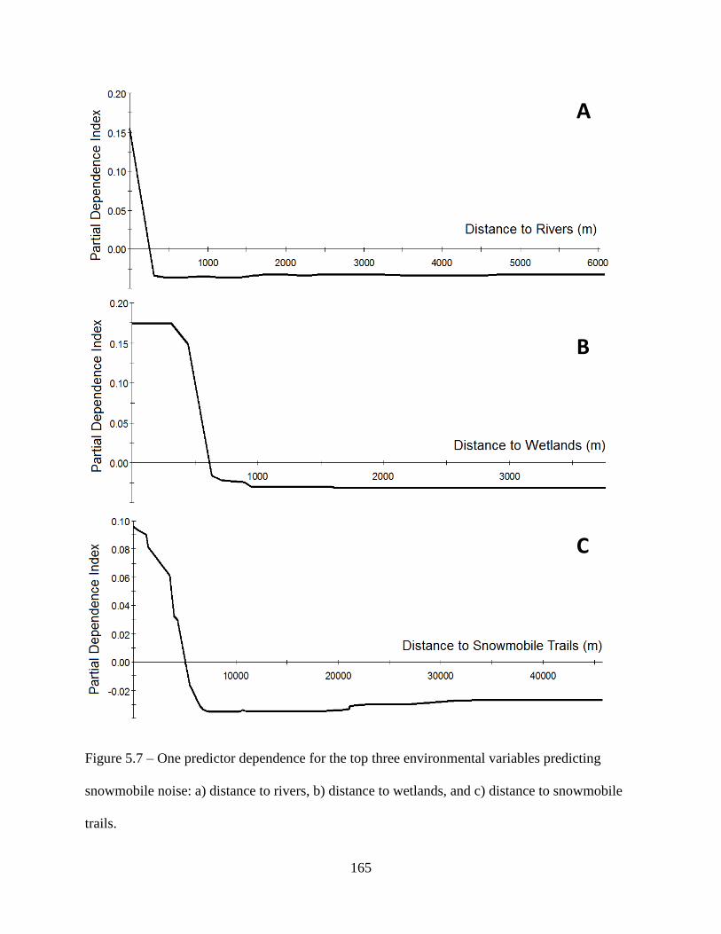
165
Figure 5.7 – One predictor dependence for the top three environmental variables predicting
snowmobile noise: a) distance to rivers, b) distance to wetlands, and c) distance to snowmobile
trails.
A
B
C

166
Figure 5.8 – Predicted distribution of snowmobile noise and the locations where moose fecal
samples were collected.

167
The AICc model averaging I conducted for my regression models to determine the
relationship between fecal GC and physiological and environmental variables indicated that 81%
of the weight was distributed between three similar models (AICc Weight <2.00; Table 5.5).
Within the top two weighted models, moose fecal GC had a significant positive relationship with
T3 (p < 0.01) and sex status (p < 0.05; Tables 5.6 and 5.7). Conversely, moose fecal GC had a
significant negative relationship with snowmobile noise for all three models (p < 0.01; Tables
5.6, 5.7, and 5.8). Moose fecal GC had a positive relationship with percent area of willow in the
top AICc weighted model (p = 0.02; Table 5.6) but did not have a significant response (p = 0.12)
in the second AICc weighted model when percent area of deciduous forest was incorporated into
the regression model. Percent area of willow was positively correlated with sex status (Pearson
= 0.298, p = 0.001) suggesting that sample locations of pregnant females had a relatively higher
percentage of willow within 1 km of the sample than males and non-pregnant females. When
percent area of willow was incorporated as an interaction term in regression models (Table 5.5),
sex status, percent area of willow, and the interaction term had a positive relationship with fecal
GC levels, although these relationships were not significantly different than zero (p > 0.05; Table
5.8). All three regression models had an R2 = 0.51.
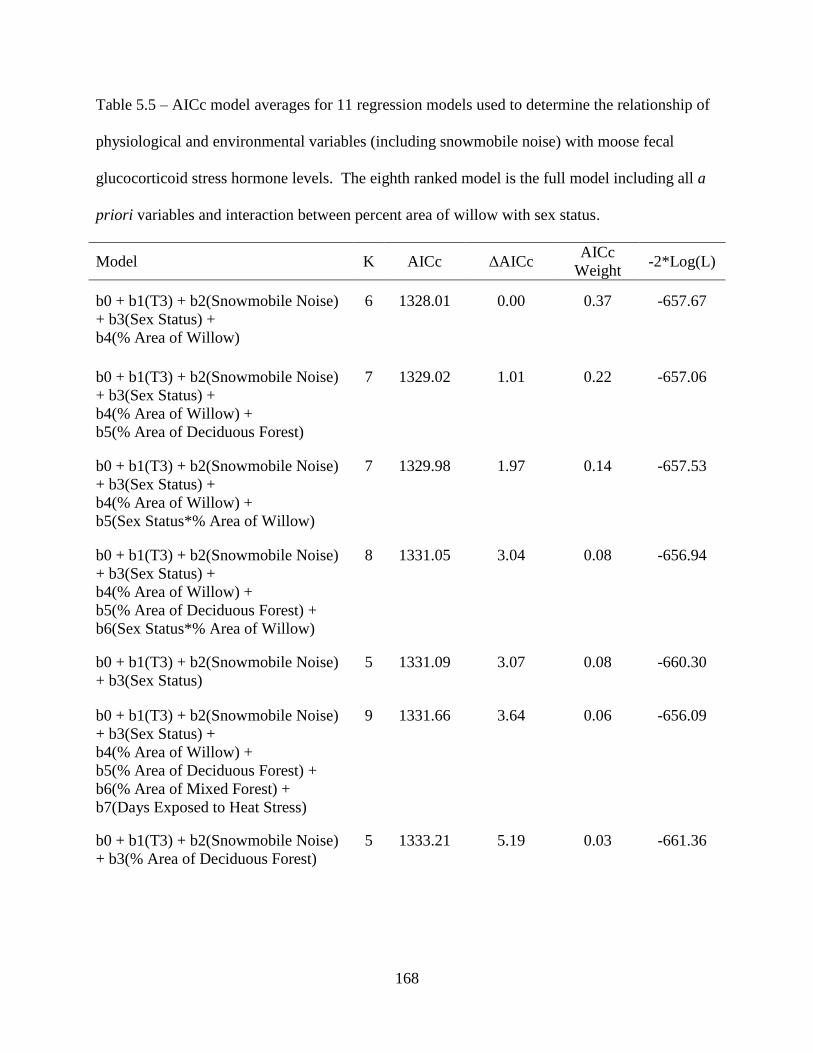
168
Table 5.5 – AICc model averages for 11 regression models used to determine the relationship of
physiological and environmental variables (including snowmobile noise) with moose fecal
glucocorticoid stress hormone levels. The eighth ranked model is the full model including all a
priori variables and interaction between percent area of willow with sex status.
Model K AICc ΔAICc AICc
Weight -2*Log(L)
b0 + b1(T3) + b2(Snowmobile Noise)
+ b3(Sex Status) +
b4(% Area of Willow)
6 1328.01 0.00 0.37 -657.67
b0 + b1(T3) + b2(Snowmobile Noise)
+ b3(Sex Status) +
b4(% Area of Willow) +
b5(% Area of Deciduous Forest)
7 1329.02 1.01 0.22 -657.06
b0 + b1(T3) + b2(Snowmobile Noise)
+ b3(Sex Status) +
b4(% Area of Willow) +
b5(Sex Status*% Area of Willow)
7 1329.98 1.97 0.14 -657.53
b0 + b1(T3) + b2(Snowmobile Noise)
+ b3(Sex Status) +
b4(% Area of Willow) +
b5(% Area of Deciduous Forest) +
b6(Sex Status*% Area of Willow)
8 1331.05 3.04 0.08 -656.94
b0 + b1(T3) + b2(Snowmobile Noise)
+ b3(Sex Status)
5 1331.09 3.07 0.08 -660.30
b0 + b1(T3) + b2(Snowmobile Noise)
+ b3(Sex Status) +
b4(% Area of Willow) +
b5(% Area of Deciduous Forest) +
b6(% Area of Mixed Forest) +
b7(Days Exposed to Heat Stress)
9 1331.66 3.64 0.06 -656.09
b0 + b1(T3) + b2(Snowmobile Noise)
+ b3(% Area of Deciduous Forest)
5 1333.21 5.19 0.03 -661.36
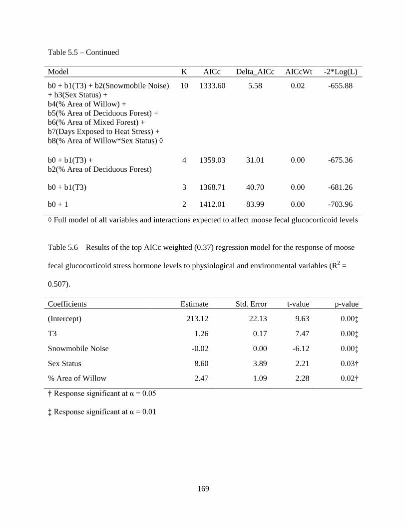
169
Table 5.5 – Continued
Model K AICc Delta_AICc AICcWt -2*Log(L)
b0 + b1(T3) + b2(Snowmobile Noise)
+ b3(Sex Status) +
b4(% Area of Willow) +
b5(% Area of Deciduous Forest) +
b6(% Area of Mixed Forest) +
b7(Days Exposed to Heat Stress) +
b8(% Area of Willow*Sex Status) ◊
10 1333.60 5.58 0.02 -655.88
b0 + b1(T3) +
b2(% Area of Deciduous Forest)
4 1359.03 31.01 0.00 -675.36
b0 + b1(T3) 3 1368.71 40.70 0.00 -681.26
b0 + 1 2 1412.01 83.99 0.00 -703.96
◊ Full model of all variables and interactions expected to affect moose fecal glucocorticoid levels
Table 5.6 – Results of the top AICc weighted (0.37) regression model for the response of moose
fecal glucocorticoid stress hormone levels to physiological and environmental variables (R2 =
0.507).
Coefficients Estimate Std. Error t-value p-value
(Intercept) 213.12 22.13 9.63 0.00‡
T3 1.26 0.17 7.47 0.00‡
Snowmobile Noise -0.02 0.00 -6.12 0.00‡
Sex Status 8.60 3.89 2.21 0.03†
% Area of Willow 2.47 1.09 2.28 0.02†
† Response significant at α = 0.05
‡ Response significant at α = 0.01
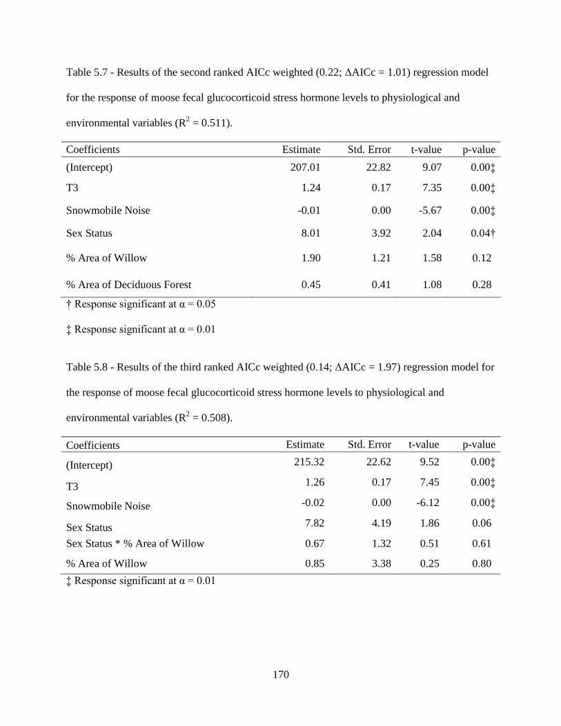
170
Table 5.7 - Results of the second ranked AICc weighted (0.22; ΔAICc = 1.01) regression model
for the response of moose fecal glucocorticoid stress hormone levels to physiological and
environmental variables (R2 = 0.511).
Coefficients Estimate Std. Error t-value p-value
(Intercept) 207.01 22.82 9.07 0.00‡
T3 1.24 0.17 7.35 0.00‡
Snowmobile Noise -0.01 0.00 -5.67 0.00‡
Sex Status 8.01 3.92 2.04 0.04†
% Area of Willow 1.90 1.21 1.58 0.12
% Area of Deciduous Forest 0.45 0.41 1.08 0.28
† Response significant at α = 0.05
‡ Response significant at α = 0.01
Table 5.8 - Results of the third ranked AICc weighted (0.14; ΔAICc = 1.97) regression model for
the response of moose fecal glucocorticoid stress hormone levels to physiological and
environmental variables (R2 = 0.508).
Coefficients Estimate Std. Error t-value p-value
(Intercept) 215.32 22.62 9.52 0.00‡
T3 1.26 0.17 7.45 0.00‡
Snowmobile Noise -0.02 0.00 -6.12 0.00‡
Sex Status 7.82 4.19 1.86 0.06
Sex Status * % Area of Willow 0.67 1.32 0.51 0.61
% Area of Willow 0.85 3.38 0.25 0.80
‡ Response significant at α = 0.01

171
5.5 Discussion
Moose exhibited a distinct spatial partitioning from areas of high snowmobile activity
and developed areas that also produce noise (i.e., oil and gas compressors). Snowmobile activity
was strongly associated with roads which provide snowmobilers access to remote areas from
multiple locations on the western borders of KENWR with urban areas and the Sterling highway.
Areas where moose and snowmobile activity overlapped were within close proximity to roads.
These areas may be sites of compounding risk to moose from the presence of both snowmobile
activity and road traffic although moose in these locations may be more behaviorally tolerant to
such activity despite the risk of disturbance. Risenhoover (1989), Rea (2003), and Laurian et al.
(2008) found this behavioral response to be true for moose commonly found browsing next to
roads. Such behavior could also be a response to direct predation risk. Some research suggests
that roads may serve to reduce moose predation by wolves (Kunkel and Pletscher 2000) and
therefore certain individuals may utilize these areas for that very reason. Regardless of the
observations in these studies, my models indicated that distance to roads was not an important
predictor of moose activity in general providing evidence that roads are not preferred areas of
activity for moose this time of year.
Snowmobile activity was also associated with high elevations. This was largely due to
the detection of a high number of snowmobile tracks in the alpine area of the Caribou Hills
located in the southwest corner of KENWR. All other areas of KENWR at high elevations
(above treeline), like those in the Kenai Mountains to the east, are restricted to snowmobiles.
Because of this restriction, I excluded the Kenai Mountains from my aerial surveys so I have no
record of illegal snowmobile activity in this region.
172
Elevation was not an important predictor of moose activity in my study area. In winter,
moose are known to move to lower elevations in response to increases in snow depth (Edwards
and Ritcey 1956). My study also supported this finding and that of others (Hundertmark et al.
1990, Dussault et al. 2005) in that moose activity was strongly associated with shallower snow
depths at lower elevations. Judging by my models’ results, with support of other studies, it is
unlikely that snowmobile activity in the Caribou Hills is affecting moose in KENWR during the
month of March.
Interestingly, I found that snowmobile activity was associated closer to willow stands.
Willow is known to be an important browse species for Alaskan moose in winter (Oldemeyer et
al. 1977, Risenhoover 1989). However, my moose activity model indicated that distance to
willow stands was not an important predictor of moose activity. Rather, moose were strongly
associated with burned areas ≤20 years old which, in turn, was not an important predictor of
snowmobile activity.
The importance of post-fire succession to moose has been documented by a number of
studies throughout their range in North America, including the Kenai Peninsula (Aldous and
Krefting 1946, Peterson 1953, Spencer and Chatelain 1953, Edwards and Ritcey 1956, Lutz
1960, Spencer and Hakala 1964, Gasaway et al. 1989, Loranger et al. 1991, and Weixelman et al.
1997). Hatter (1949) and Cowan et al. (1950) reported that the seral brush fields of post-fire
succession provided moose in British Columbia with a variety of palatable browse species.
MacCracken and Viereck (1990) found that high quality browse for moose occurred within a few
years post-fire yet nutrient content declined as years post-fire progressed. It is evident from
these models that moose are generally selecting relatively early seral stages of post-fire habitat
where snowmobiles do not occur. Due to the proximity of snowmobile activity to willow stands

173
and the association of moose to burn areas indicated in my models suggests that willow stands in
areas of snowmobile activity are not preferred by moose. These results may imply that willow
habitats are not available to moose in the presence of snowmobile disturbance.
Moose are known to select habitats based on limiting factors such as food availability,
snow conditions, and predation (Dussault et al. 2005). Given that my models predicted moose
were strongly selecting burn areas and sites where snow depth was <60 cm support the findings
of Dussault et al. (2005). However, moose were also found to select areas with little to no
snowmobile activity and further away from oil and gas compressors. These latter results suggest
that moose are avoiding these areas and perhaps add an additional factor in how moose are
selecting winter habitats in March.
It should be noted that my snowmobile activity model does not reflect the amount of
snowmobile activity along established trails or along rivers but represents the activity of less
restricted free-ranging snowmobiles. Free-ranging snowmobile activity could be more pervasive
and threatening to moose than predictable activity along trails. This may explain one of the
factors involved in moose habitat selection this time year.
Despite my snowmobile activity model’s representation of such activity along
established trails, I was able to sample the physiological response of moose to varying intensities
of snowmobile traffic along established trails. My results indicate that moose fecal GC levels
did not significantly differ between snowmobile traffic levels of <5 passes, 5-10 passes, and >10
passes within a 10 day period of sample collection. Colescott and Gillingham (1998) found that
moose do respond to snowmobile activity along trails by moving away from the area in response
to oncoming traffic. In their study, moose typically moved away from trails as the day
progressed but not necessarily in response to snowmobile traffic. This observed behavior may
174
be due to a shift in normal daily activity. My results in comparison to that of Colescott and
Gillingham (1998) suggest that moose response to snowmobile traffic along trails is short-lived
and likely less susceptible to more chronic effects of snowmobile disturbance if their activity is
not centered within the vicinity of the trail itself. This would account for the lack of
comparatively higher fecal GC levels than moose in quieter areas. I recognize that the time
interval of snowmobile passes could also have some affect on fecal GC levels where 10
snowmobile passes within a short period of time (e.g., one day) could have a different affect on
moose stress response than a single snowmobile pass everyday for 10 days. This would also be
true for the vicinity of moose to such differences in activity along trails. Regardless, the amount
of snowmobile activity did not exceed 12 snowmobile passes within a 10 day period. This level
of activity is quite low compared to very active trails in the Caribou Hills that can have triple this
amount of activity within a 10-day period.
My snowmobile noise model predicted a much wider area affected by snowmobiles
compared to my snowmobile activity model, making it a more realistic depiction of where
snowmobiles occur throughout the entire winter. This is evidence that sound is a good indicator
of human disturbance. My analysis of moose fecal GC response to snowmobile noise revealed
that noise was not a significant factor in elevating stress hormone levels in areas I sampled.
Many of my samples were located along snowmobile trails where snowmobile noise was
strongly associated. Although moose exhibited comparatively lower fecal GC levels than moose
in quieter areas, they were typically within areas with less preferred food (i.e., willow) and had
lower T3 concentrations, an indicator of nutritional stress.
Conversely, moose in quieter areas exhibited higher fecal GC levels but were within
areas with higher percent area of willow and higher T3 concentrations. This finding contradicts

175
those of others where higher fecal GC levels were associated with lower T3 (Wasser et al. 2011).
However, Taillon and Côté (2008) found that white-tailed deer fawns who fed on a higher
quality control diet exhibited higher fecal GC levels than fawns feeding on low quality diet.
They supposed that fawns feeding on the control were evidently nutritionally stressed despite the
quality of the diet. Since T3 is known to be a direct measure of nutritional status (Wasser et al.
2011) my results do not fully support the logic of Taillon and Côté (2008).
It is known that the concentrations of GC affect an animal’s food intake (Wingfield 2005,
Barboza et al. 2009). Mild distress resulting in slight rises in GC can cause an animal to increase
feeding in order to meet the anticipated demand. Overfeeding and obesity has also been
associated with chronic low elevations in GC (Wingfield 2005). However, high concentrations
of GC will suppress food intake as well as other physiological effects on the immune response
otherwise decreasing the energy needed to maintain homeostasis (Barboza et al.2009) which
ultimately results in nutritional stress (i.e., lower T3).
One possibility of why my results contradict that of the literature may be due to the type
of assay used to acquire fecal GC concentrations. In particular, the high concentrations of T3
suggest that moose in these quieter areas have a higher quality diet than those moose in areas
where snowmobile noise is high. This would indicate that moose in quieter areas are consuming
more digestible food matter. If moose are therefore excreting less food waste but normal levels
of GC then fecal GC concentrations would be considered higher than that of GC concentrations
in pellets consisting of more food waste (i.e., less digestible material) from individuals with a
lower quality diet (P. Barboza, University of Alaska Fairbanks, pers comm.). Unfortunately, my
samples were destroyed before I could have an additional analysis done on the amount of
digestible material in my samples to test this hypothesis post hoc.
176
Conversely, sex status was also significantly positively related to increasing fecal GC
levels. Handa et al. (1994) and Kejantie (2006) reported that corticosterone levels vary
considerably between males and females and increase with increasing levels of progesterone.
Pregnant females are especially known to have higher corticosterone levels when compared to
non-pregnant individuals (Oettel and Mukhopadhyay 2004). I had categorized my sex status
based on progesterone levels. Progesterone in males was not necessarily a factor in determining
sex but was specifically identified during the immunoassay using DNA. Therefore, I categorized
my sex status by giving males a value of 1, non-pregnant females a value of 2, and pregnant
females a value of 3. The latter two categories were assigned based on a distinct separation
between low and high progesterone levels (Fig 5.1). Given these categories and the positive
relationship between fecal GC and sex status, I can conclude that pregnant moose were
exhibiting higher fecal GC levels when incorporated with other environmental and physiological
variables in my models. These results support the findings of others (Handa et al. 1994, Oettel
and Mukhopadhyay 2004, Kejantie 2006). Additionally, sex status of the moose I sampled was
positively correlated with percent area of willow suggesting that pregnant females were within
proximity to more available willow habitat in areas in quieter areas. Although T3 was not
correlated with sex status, the known increases in fecal GC levels that coincide with
progesterone levels and pregnancy status could be confounding the relationship between fecal
GC levels with T3 and percent area of willow that were indicated in my regression models.
Gill et al. (2001) postulated that wildlife in a human disturbed environment will make
decisions to move to alternative habitats with low or no disturbance based on the quality of their
present habitat and that of alternative habitats. Also, Webb and Blumstein (2005) found that
there was individual variation in animal response to various levels of human disturbance. They
177
concluded that more tolerant individuals of disturbance are less likely to leave the disturbed area
than individuals who were less tolerant. These conclusions indicate that an individual’s
perception of risk and the quality of their habitat is highly dependent on their tolerance to
disturbance and thus influences their decision to move to alternative areas.
Based on my findings, moose closer to snowmobile trails exhibited a higher
physiological tolerance (i.e., habituation) to snowmobile disturbance of both traffic exposure and
noise but their decision to stay in a lower quality habitat, in terms of nutritional forage, was
confounded by factors other than the ones I measured, such as the availability of alternative
habitats and risk of predation. The true quality of habitats along snowmobile trails and that of
alternative habitats, in addition to the activity patterns of predators and rate of predation on
moose in these areas, would prove a useful measure to understanding the behavior of moose who
select habitats within the vicinity of snowmobile trails. The same information would also be
useful in understanding the nutritional and stress status of moose further from snowmobile trails
and in areas with less snowmobile noise.
Interestingly though, in a broader spatial context of moose activity across the landscape
of KENWR in relation to snowmobile activity, my results provide evidence that the distribution
of moose is influenced by the less restricted activity of free-ranging snowmobiles. The
physiological response of the particular moose I sampled within the vicinity of snowmobile trails
may only reflect individual variation in habitat selection rather than broader population-level
responses. This broader spatial effect could have more overreaching impacts on KENWR’s
moose population, as well as ecological processes (Senft et al. 1987).
The Kenai National Wildlife Refuge encompasses Game Management Unit 15 (GMU)
which consists of three subunits (15A, 15B, and 15C). Historically, environmental conditions

178
have been favorable for moose. The near absence of predators and a large 130,000 ha fire in
1947 contributed to favorable habitat and low mortality through the 1950s and 1960s in GMU
15A. Despite evidence that moose populations have been relatively stable over the years in
GMU 15B, more recently moose populations in GMU 15A and 15C have seen considerable
declines (Harper 2011). This decline is largely due to loss of habitat and low frequency and area
of fire. Preferred browse species associated with post-fire succession has been lacking in recent
years while forests take over historic burn areas, pressure from predators persists, and human
population growth and development continue to increase.
The potential for moose populations to grow will largely depend on fire and the
succession of vegetation of preferred browse. My moose activity model is a good indication that
moose are utilizing burn areas that have occurred within the last 20 years. Several fires in GMU
15B were predicted as high activity areas for moose and are likely contributing to the stability of
moose populations in this area. More recently, a 78,000 ha fire burned the Funny River region in
May 2014 between Skilak and Tustumena Lakes of GMU 15B. High and medium levels of
moose activity were predicted in this area two winters prior to this fire. Although immediate
effects of this fire on moose could be negative, this burn area will likely contribute to the moose
population in GMU 15B in the future.
Harper’s (2011) report on the status of moose in GMU 15C suggested that the Fox Creek
Fire that burned in 2005 would likely become an important site for moose by 2015. My model
results support this projection in that moose activity was high within this specific burn area.
Unfortunately, fire in GMU 15A has been extremely low within the last 20 years contributing to
the decline of moose in this region.

179
Snowmobile activity may be an additional factor to moose habitat selection in winter but
there are many other variables involved that are affecting the KENWR’s moose population.
Stress in these animals is also dependent on a number of factors. Several studies have reported
the benefits of fecal GC analysis as a non-invasive measure of the effects of human disturbance
on wildlife (Tomeo 2000, Creel et al. 2002, Möstl and Palme 2002, Freeman 2008, Sherriff et al.
2011, Wasser et al. 2011). However, a few publications have raised questions on the validity of
fecal GC metabolites as an effective metric of wildlife hormonal responses to specific stimuli
due to the variety of factors that influence fecal GC levels (Millspaugh and Washburn 2004,
Touma and Palme 2005, Goyman 2012).
I attempted to account for as much variation in my moose stress response with
environmental and physiological predictor variables with the resources I had available. The
variables I used in my analysis accounted for 51% of the variation in my samples for the top
AICc weighted regression models. Although I am confident that the results of my models
captured an important interpretation of the response of moose fecal GC levels to snowmobile
noise, I recognize that there were additional variables that influenced my moose stress levels that
I did not measure.
Particularly, I did not obtain data on the exact number of individuals I collected from.
Presumably, since many of my samples were within the vicinity of snowmobile trails, it is
possible that the number of individuals I was sampling from was small. I cannot assume,
however, that my results reflect individual variation. Second, I did not account for predator
activity or predation risk although all my samples were collected within the boundaries of known
wolf territories. Third, my fecal samples were not randomly distributed. My study design was to
sample moose pellets within the vicinity of my sound stations which were spatially stratified.

180
Nevertheless, only a few areas where I recorded did I find moose pellets, otherwise limiting the
area I could infer my results. Fourth, I did not have samples from a control population that could
presumably be used as a reference for natural variation in fecal GC without disturbance. Finally,
I had a relatively small sample size.
Combined with the lack of knowledge on the number of individuals I had collected from,
my small sample size may not be representative to the larger moose population. Conversely, the
amount of variation I was able to capture with the physiological and environmental variable
relationships with moose fecal GC suggest there is evidence that moose located next to
snowmobile trails generally have lower levels of stress hormone yet are nutritionally stressed in
these areas. This study should at least attest to the need for further, more intensive study in order
to make broader inferences.

181
CHAPTER 6
ASSESSMENT OF THE ECOLGICAL EFFECTS OF SNOWMOBILES
6.1 Conclusions
Winter is a time period when plants and animals must adapt to the stressors of freezing
temperatures (Kacperska-Palacz 1978, Marchand 1996), snow (Marchand 1996, LeResche 1974,
Bunnell et al. 1990, Hundertmark et al. 1990), and the reduction and altered nutritional state of
food (Bryant and Kuropat 1980). These forcing functions have been strong selective factors in
the evolution of plants and animals in subarctic boreal ecosystems. These species have only
recently been subjected to the forcing functions of human-mechanized disturbance.
Furthermore, disturbance to plants and wildlife by snowmobiles has only become of concern
within the last 50 yrs which is not nearly enough time for species to evolve effective adaptive
strategies to counter its effects. Rather, plants and wildlife must rely solely on the physiological
and behavioral adaptations that natural processes have currently selected for.
The results of this study indicate that dwarf birch, shrubby cinquefoil, and sweet gale
were not resilient to the effects of snowmobile traffic as one might expect with snow depths
reaching an excess of 67 cm. The site-specific impacts of snowmobile traverses on wetland
shrubs could extend further to other wetland areas used by snowmobilers. The KENWR has
approximately 6,509 ha of shrub-dominated wetlands, much of which is affected by snowmobile
activity, as detected by sound monitoring. In these areas, snowmobiles not only have the
potential to directly affect the vegetation community but also indirectly affect other ecological
components through disturbance of the sonic environment.

182
Moose appeared to be affected at a landscape-level by the activity of free-ranging
snowmobiles based on their distinct spatial separation. However, moose located closer to
snowmobile trails did not exhibit a marked physiological response to varying degrees of
snowmobile traffic intensity or snowmobile noise associated with these areas. The physiological
stress response of moose to disturbance, whether human-related or by predators, is an adaptive
strategy to increase survival (Wingfield et al. 1998). This emergency life-history response to
changes in the environment is what allows moose to adapt to changes in homeostasis caused by a
stressor (Wingfield et al. 1998). The noise and presence of a snowmobile along an established
trail could be perceived as less threatening to moose than the same disturbance in an open, less
restricted and less predictable environment. Therefore, differential response to snowmobile
activity is expected due to an individual’s or group’s perception of the disturbance as threatening
or previous experience with the same source of disturbance (Westman and Walters 1981).
Furthermore, an animal’s decision to leave an area to avoid snowmobile disturbance is also
dependent on the availability of surrounding, alternative habitats (Gill et al. 2001). Areas where
moose occur within areas of snowmobile activity beyond snowmobile trails where there activity
is less predictable are probably sites where the impact from snowmobile activity is most
pronounced perhaps resulting in animal’s spatial reorientation to other available habitats (e.g.,
burn areas) to avoid the disturbance as winter progresses.
Despite these effects of snowmobile activity on plants and wildlife, it was interesting to
find that the winter soundscape of KENWR was dominated by silence and geophony, indicating
that KENWR was primarily quiet and acoustically uneventful (in terms of biological activity)
throughout much of winter. Relative to other anthrophonic sound sources, snowmobile noise
was not a large contributor to the entire winter soundscape of KENWR. However, unlike the
183
anthrophonic sound sources derived from infrastructure (e.g., road and compressor noise), I
found that the acoustic footprint of snowmobile noise extends well into wilderness areas where
natural sounds typically dominate. Certainly this acoustic disturbance is not continuous but
occurs intermittently making the disturbance that much more unexpected although short-lived.
The natural processes that are being affected by this noise are not yet realized. My results do
show, however, that 17% of all Congressionally-designated Wilderness areas were affected by
snowmobile noise and 32% of Wilderness areas open to snowmobiling were disturbed by
snowmobile noise. Most of these Wilderness areas were typically within 15 km from roads or
snowmobile trails. This is further support that roads and trails used for access into and
throughout KENWR by snowmobilers contributes to a broader spatial effect to Kenai Wilderness
and the sonic environment than the confines of developed areas. Additionally, other studies that
have focused on noise affects on wildlife indicate anthrophony has significant negative effects on
vocal species (Ortega 2012, Ortega and Francis 2012, Barber et al. 2010, Dooling and Popper
2007, Habib et al. 2007). The fact that I found a small proportion of biophony occurring
simultaneously with anthrophony suggests that further study could reveal similar results.
Of all the outdoor recreational vehicles, snowmobiles may be thought of as the most
benign to the environment because they traverse over a snow covered substrate that melts in the
spring suggesting that their impression and impact on the environment is erased. However, the
results of my research provide evidence that snowmobile activity does affect the environment. I
found that snowmobile activity reduced the number of living stems and inhibited the growth of
woody wetland plants by direct contact with protruding vegetation above the snow and indirectly
from snow compaction. Snowmobile noise was not a large contributor of noise to the
soundscape but was pervasive in remote natural areas. Snowmobile noise affected a significant

184
area of Congressionally-designated wilderness altering the naturalness and character of the
wilderness soundscape. Moose exhibited a distinct spatial partitioning and avoidance from
snowmobile activity and developed areas (i.e., oil and gas compressors) at the landscape-level
but at a site-specific scale snowmobile traffic and noise had no apparent affect on the stress
hormone levels of moose that were selecting habitats close to snowmobile trails (Table 6.1). I
detected these impacts at both site-specific locations and across large spatial scales indicating
that snowmobile effects are more than just localized disturbances.
It should be noted that my work on vegetation responses to snowmobile traverses and
moose spatial and physiological responses to snowmobile activity and noise can be considered
conservative outcomes to the long-term, varying intensities of snowmobile use across KENWR.
Snowmobile activity has been occurring in the area for nearly 50 yrs and my results are just a
snapshot of the site-specific and landscape-scale impacts that have already formed over the
course of this time frame. Hence, vegetation communities may already be altered and moose
populations may have already made behavioral decisions to counter act the effects of this already
disturbed environment. Projections on population growth in the area are increasing and the use
of snowmobiles in KENWR is likely to increase as well, ultimately compounding the effects I
found (Comprehensive Conservation Plan 2010).
I conclude that snowmobile activity in the Kenai National Wildlife Refuge is an
additional forcing function on important state variables such as wetland vegetation and moose
winter distributions that are both significant components in ecological systems. My results show
that the state of snowmobile activity in KENWR not only has a lower impact to moose along
snowmobile trails and the alpine region of the Caribou Hills, but the effects of free-ranging
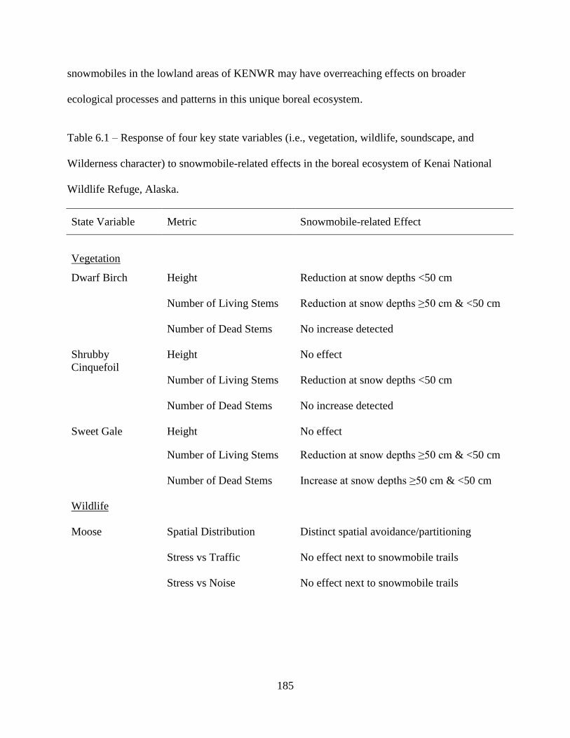
185
snowmobiles in the lowland areas of KENWR may have overreaching effects on broader
ecological processes and patterns in this unique boreal ecosystem.
Table 6.1 – Response of four key state variables (i.e., vegetation, wildlife, soundscape, and
Wilderness character) to snowmobile-related effects in the boreal ecosystem of Kenai National
Wildlife Refuge, Alaska.
State Variable Metric Snowmobile-related Effect
Vegetation
Dwarf Birch Height Reduction at snow depths <50 cm
Number of Living Stems Reduction at snow depths ≥50 cm & <50 cm
Number of Dead Stems No increase detected
Shrubby
Cinquefoil
Height No effect
Number of Living Stems Reduction at snow depths <50 cm
Number of Dead Stems No increase detected
Sweet Gale Height No effect
Number of Living Stems Reduction at snow depths ≥50 cm & <50 cm
Number of Dead Stems Increase at snow depths ≥50 cm & <50 cm
Wildlife
Moose Spatial Distribution Distinct spatial avoidance/partitioning
Stress vs Traffic No effect next to snowmobile trails
Stress vs Noise No effect next to snowmobile trails

186
Table 6.1 – Continued
State Variable Metric Snowmobile-related Effect
Soundscape Proportion of Soundscape Contributed to 3% of entire soundscape
Wilderness
Character
Proportion of Area
Affected
Affected 32% of unrestricted Wilderness
Affected 0% of restricted Wilderness
Affected 17% of total Wilderness
6.2 Management Recommendations
The Kenai National Wildlife Refuge is under mandate of the National Wildlife Refuge
System Administration Act of 1966, as amended (16 U.S.C. 668dd-668ee) and the National
Wildlife Refuge System Improvement Act of 1997 (Public Law 105-57) to assess the
compatibility of recreational activities with that of its mission. The Alaska National Interests
Lands Conservation Act of 1980 also states that one of the purposes of KENWR is to provide in
a manner compatible with the management of fish and wildlife resources, opportunities for fish
and wildlife oriented recreation (Sections 303(4)(i) and 303(4)(v)). ANILCA also specifies the
allowable use of snowmobiles in KENWR and Kenai Wilderness (Sections 1110(a) and 811(b)).
Current regulations on snowmobiles in KENWR are: 1) prohibited use of Swanson River
and Swan Lake Canoe Routes and alpine areas of the eastern Kenai Mountains, 2) snowmobiles
are not allowed for assistance in big game hunting, 3) no use of maintained roads, 4) the size of
snowmobiles is restricted to be less than 100 cm wide, and 5) no racing or harassment of
wildlife.
One of the most potentially useful restrictions to limit the impacts of snowmobiles to
plants and animals is the time of use and judgment of adequate snowfall by the KENWR

187
Manager. Currently KENWR does not consider opening to snowmobiling until December 1st
and closes no later than April 30th
. These decisions are weighted heavily on what law
enforcement officers judge to be adequate snow conditions (R. Barto, KENWR law enforcement
officer, per comm.). Unfortunately, due to the enthusiasm of many snowmobile club members
and public recreationists the KENWR Manager is oftentimes subject to considerable social
pressure to open KENWR despite what would be considered adequate snow fall (2007
Compatibility Determination).
The results of my study suggest that what has typically been considered to be adequate
snow depth (≥30 cm) for protecting underlying vegetation is not entirely sufficient for prevalent
wetland shrub species. Additionally, the fact that snow depth varies considerably throughout the
landscape and over time suggests that “adequacy” is more subjective to an individual’s or
group’s interpretation. Should the KENWR Manager continue to open snowmobiling based on
adequate snow depth he/she must strongly consider the spatial distribution of snow, areas of
potentially high snowmobile use (namely wetlands and the Caribou Hills), the vegetative species
he/she deems important for conservation efforts, and a continued monitoring effort of snow
depth across all areas open to snowmobiling throughout winter.
This suggestion is certainly a possibility due to the presence of aerial snow markers I
distributed throughout KENWR in 2009 (Appendix 2). Monitoring the spatial distribution of
snow depth along with on-site measurements by law enforcement would provide a more reliable
assessment of the adequacy of snow depth to ensure that underlying vegetation is provided
sufficient protection from free-ranging snowmobile activity.
A second option is to establish trails where snowmobile users can conduct “fish and
wildlife oriented recreation.” My study supports the hypothesis that snowmobile-related effects

188
are more pronounced when their activity ranges freely throughout the landscape along rivers and
throughout wetlands than when snowmobile activity is restricted and predictable on already
available snowmobile trails (e.g., Mystery Creek Road and Hansen and Funny River Horse
Trails). I believe wildlife and vegetation in the lowland areas of KENWR would benefit the
most from designated trails due largely on the tendency of snow depths to be more variable and
wildlife to be more prevalent in areas further from snowmobile trails. This would otherwise
minimizing the impact zone by designating areas for snowmobile use that can be easily
maintained, managed, and monitored.
The Caribou Hills region of KENWR in the southwest has been an area of growing
snowmobile recreational activity. The region outside KENWR consists of a very well-
maintained network of trails lined with a growing number of cabins constructed by a cohesive
community of snowmobile users. With the vast, treeless landscape of Caribou Hills managed by
KENWR, snowmobilers are free to maneuver unimpeded. This well-sought after experience has
become the foundation of a growing subculture of recreational snowmobile users called the
Caribou Hills Cabin Hoppers.
Parking lot surveys I conducted in the Caribou Hills over the course of six weekends for
two winters along Oil Well Road showed that 68% of the snowmobiles I was able to identify to
model were high-performance vehicles (51% of these were Polaris RMKs; Appendix 4). The
main purpose of these high-performance machines is to maneuver through deep snow in
backcountry settings for recreational purposes. According to www.polaris.com/en-
us/snowmobiles/rmk, Polaris RMKs are advertised as giving the user a snowmobile that is the
“lightest, strongest, and most flickable” and provides the opportunity to “ride harder and own the
mountain like never before (accessed 2014 September 12).” The popularity of this machine for

189
use in the Caribou Hills and the growing population of users is a strong indication that the
Caribou Hills is not necessarily being used for fish and wildlife oriented recreation.
Despite this evidence, I found that moose were not affected by snowmobile activity in
this area and that the soundscape in this region was largely dominated by high winds, perhaps
mitigating the effects by masking the noise snowmobiles emit. Additionally, the Caribou Hills
gets a considerable amount of snow fall compared to the lowland areas of KENWR making
snowmobile effects on vegetation less likely than what I observed in my wetland shrub
experiment. It is conceivable that the direct effects of snowmobile activity to plants and moose
in the Caribou Hills are minimal. However, that is not to say that other species may be affected.
In close regard to this situation, I recommend that the KENWR Manager define “traditional
activities,” as mentioned in ANILCA, to make his/her mission on the management of
snowmobile activity in the Caribou Hills clear to KENWR staff and the public. By minimizing
impacts within the management capabilities of KENWR staff and clarifying the mandates of
KENWR for public access is imperative to successfully fulfill the mission and purposes of this
unique and diverse system of human-nature relationships.
Finally, The National Wildlife Refuge System Administration Act of 1966, as amended
(16 U.S.C. 668dd-668ee) states that:
The Secretary is authorized, under regulations as [s]he may prescribe, to permit
the use of any area within the [National Wildlife Refuge] System for any purpose,
including but not limited to hunting, fishing, public recreation and
accommodations, and access wherever [s]he determines that such uses are
compatible.
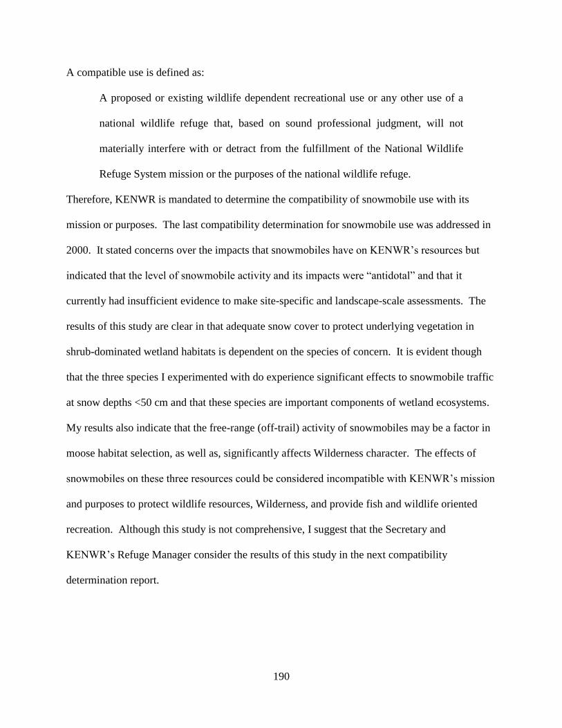
190
A compatible use is defined as:
A proposed or existing wildlife dependent recreational use or any other use of a
national wildlife refuge that, based on sound professional judgment, will not
materially interfere with or detract from the fulfillment of the National Wildlife
Refuge System mission or the purposes of the national wildlife refuge.
Therefore, KENWR is mandated to determine the compatibility of snowmobile use with its
mission or purposes. The last compatibility determination for snowmobile use was addressed in
2000. It stated concerns over the impacts that snowmobiles have on KENWR’s resources but
indicated that the level of snowmobile activity and its impacts were “antidotal” and that it
currently had insufficient evidence to make site-specific and landscape-scale assessments. The
results of this study are clear in that adequate snow cover to protect underlying vegetation in
shrub-dominated wetland habitats is dependent on the species of concern. It is evident though
that the three species I experimented with do experience significant effects to snowmobile traffic
at snow depths <50 cm and that these species are important components of wetland ecosystems.
My results also indicate that the free-range (off-trail) activity of snowmobiles may be a factor in
moose habitat selection, as well as, significantly affects Wilderness character. The effects of
snowmobiles on these three resources could be considered incompatible with KENWR’s mission
and purposes to protect wildlife resources, Wilderness, and provide fish and wildlife oriented
recreation. Although this study is not comprehensive, I suggest that the Secretary and
KENWR’s Refuge Manager consider the results of this study in the next compatibility
determination report.

191
Literature Cited
Aarts H, Dijksterhuis A. 2003. The silence of the library: environment, situational norm, and
social behavior. J of Pers Soc Psychol 84:18-28.
Aldous SE, Krefting LW. 1946. The present status of moose on Isle Royale. Transactions of the
North American Wildlife and Natural Resources Conference 11:296-308.
Anderson R, Linnell JDC, Langvatn R. 1996. Short term behavioural and physiological response
of moose Alces alces to military disturbance in Norway. Biol Conserv 77:169-176.
Assagioli R, Anglada VB. 2013. The spiritual significance of silence: two writings. Esoteric
Quart. 9:77-84.
Babisch W. 2000. Traffic noise and cardiovascular disease: Epidemiological review and
synthesis. Nois Health 8:9-32.
Babisch W, Ising H, Gallacher JE, Sweetnam PM, Elwood PC. 1999. Traffic noise and
cardiovascular risk: The Caerphilly and Speedwell studies, third phase—10 year follow
up. Arch Environ Health 54:210-216.
Ballard WB, Whitman JS, Reed DJ. 1991. Population dynamics of moose in south-central
Alaska. Wildlife Monogr 114:3-49.
Baltensperger AP, Mullet TC, Schmid MS, Humphries GRW, Kövér L, Huettmann F. 2012.
Seasonal observations and machine-learning-based spatial model predictions for the
common raven (Corvus corax) in the urban, sub-arctic environment of Fairbanks, Alaska.
Polar Biol. DOI 10.1007/s00300-013-1376-7.
Barber JR, Fristrup KM. 2010. Evaluating the prevalence of masking as a causal factor in
wildlife responses to noise. J Acoust Soc Am 127:1802.
192
Barber JR, Crooks KR, Fristrup KM. 2010. The costs of chronic noise exposure for terrestrial
organisms. Trends Ecol Evol 25:180-189.
Barboza PS, Parker KL, Hume ID. 2009. Integrative wildlife nutrition. Berlin, Germany:
Springer-Verlag. 342 p.
Belovsky GE, Jordan PA. 1978. The time-energy budget of moose. Theor Popul Biol 14:76-104.
Bjornlie DD, Garrott RA. 2001. Ecological effects of winter road grooming on bison in
Yellowstone National Park. J Wildlife Manage 65:423-435.
Boarman WI. 2003. Managing a subsidized predator population: reducing common raven
predation on desert tortoises. J Environ Manage 32:205-217.
Bolduc R, Pesant A, Drapeau R. 1977. Adaptation à l’hiver et rendement potential de quelques
luzernières du Québec au cours de l’hiver 1973-74 et 1974-75. Can J Plant Sci 57:883-
889.
Bollinger JG, Ronsgstad OJ. 1973. Snowmobile Noise effects on wildlife. Engineering and
Experiment Station. Madison(WI): University of Wisconsin. 85 p.
Bowles AE. 1995. Response of wildlife to noise. Knight, RL, Gutzwiller KJ, editors. Wildlife
and recreationists: Coexistence through management and research. Washington (D.C.):
Island Press. 109-156 p.
Boyle SA, Samson FB. 1985. Effects of nonconsumptive recreation on wildlife: a review.
Wildlife Soc B 13:110-116.
Brandenberger G, Follenius M, Wittersheim G, Salame P. 1980. Plasma catecholamines and
pituitary adrenal hormones related to mental task demand under quiet and noise
conditions. Biol Psychol 10:239-252.

193
Brumm H. 2004. The impact of environmental noise on song amplitude in a territorial bird. J
Anim Ecol 73:434-440.
Brumm, H. 2006. City birds have changed their tune. Curr Biol 16:1003-1004.
Bryant JP, Kuropat PJ. 1980. Selection of winter forage by subarctic browsing vertebrates: the
role of plant chemistry. Annu Rev Ecol Syst 11:261-285.
Bubenik AB. 1997. Behavior. Fanzmann, W, Schwartz CC, editors. Ecology and management of
the North American moose. Washington (D.C.): Wildlife Management Institute. 173-221
p.
Bunnell FL, Parker KL, McNay RS, Hovey FW. 1990. Sinking depths of black-tailed deer in
snow, and their indices. Can J Zoolog 68:917-922.
Bunnell KD, Flinders JT, Wolfe ML. 2006. Potential impact of coyotes and snowmobile on lynx
conservation in the Intermountain West. Wildlife Soc B 34:828-838.
Burkowski JJ, White PJ, Garrott RA, Davis T, Hardy AR, Reinhart DJ. 2006. Behavioral
responses of bison and elk in Yellowstone to snowmobiles and snow coaches. Ecol Appl
16:1911-1925.
Burnham KP, Anderson DR. 2002. Model selection and multimodel inference: a practical
information-theoretic approach. 2nd
ed. New York (NY): Springer-Verlag. 488 p.
Burson S. 2008. Natural soundscape monitoring in Yellowstone National Park December 2007-
March 2008. Yellowstone Center for Resources. USGS. 106 p.
Butler J. 1970. Snowmobile Sales Up-Swing Defies Slowing Economy. Michigan Snowmobiler.
194
Cai T, Huettmann F, Guo Y. Using stochastic gradient boosting to infer stopover habitat
selection and distribution of Hooded Cranes Grus monacha during spring migration in
Lindian, Northeast China. PLoS ONE 9 [Internet]: 2014 [cited 2014 August 8]; 9.
Available from: doi: 10.1371/journal.pone.0097372
Caissie A. 1991. Effects of snowmobile traffic on the vegetation of coastal plain Sphagnum bog
in Gros Morne National Park, western Newfoundland. M.S. Thesis. University of New
Brunswick. 266 p.
Ceballos G, Ehrlich PR. 2002. Mammal population losses and the extinction crisis. Science
296:904-907.
Christensen TR, Jonasson S, Callaghan TV, Havström M. 1999. On the potential CO2 release
from tundra soils in a changing climate. Appl Soil Ecol 11:127-134.
Clark C, Sörqvist P. 2012. A 3 year update on the influence of noise on performance and
behavior. Nois Health 14:292-296.
Cmiel CA, Karr DM, Gasser DM, Oliphant LM, Neveau AJ. 2004. Noise control: A nursing
team’s approach to sleep promotion: respecting the silence creates a healthier
environment for your patients. Am J Nurs 104:40-48.
Colescott JH, Gillingham MP. 1998. Reaction of moose (Alces alces) to snowmobile traffic in
the Grays River Valley, Wyoming. Alces 34:329-338.
Collins WB. 2002. Interrelationship of forage and moose in game management unit 13, 1 July
1995-30 June 2001. Alaska Department of Fish and Game Research Federal aid in
wildlife restoration research final performance report. Juneau, Alaska. 22 p.

195
Compatibility Determination. 2007. Kenai National Wildlife Refuge determination of the
compatibility of snowmachine use with Refuge mission. Soldotna (AK): Department of
Interior, U.S. Fish and Wildlife Service, Kenai National Wildlife Refuge, Region 7.
Comprehensive Conservation Plan. 2010. Soldotna (AK): Department of Interior, U.S. Fish and
Wildlife Service, Kenai National Wildlife Refuge, Region 7.
Cowan IM, Hoar VC, Hatter J. 1950. The effect of forest succession upon the quantity and upon
the nutritive values of woody plants used as forage by moose. Can J Zoolog 28:249-271.
Craig E, Huettmann F. 2009. Using “blackbox” algorithms such as TreeNet and Random Forests
for data-mining and for meaningful patterns, relationships and outliers in complex
ecological data: an overview, an example using golden eagle satellite data and an outlook
for a promising future. In Wang, HF, editor. Intelligent data analysis: developing new
methodologies through pattern discovery and recovery. Hershey (PA): Idea Group Inc.
65-67 p.
Creel S. 1997. Handling of African wild dogs and chronic stress: Reply to East et al. Conserv
Biol 11:1454-1456.
Creel S, Fox JE, Hardy A, Sands J, Garrott B, Peterson RO. 2002. Snowmobile activity and
glucocorticoid responses in wolves and elk. Conserv Biol 16:809-814.
Crutzen PJ. 2006. The anthropocene. Ehlers, E, Krafft T, editors. Earth System Science in the
Anthropocene: Emerging issues and problems. New York (NY): Springer. 13-18 p.
Cutler DR, Edwards TC, et al. 2007. Random forests for classification in ecology. Ecology
88:2783-2792.
Cyr NE, Romero LM. 2009. Identifying hormonal habituation in field studies of stress. Gen
Comp Endocr 161:295-303.
196
Daan S, Aschoff J. 1975. Circadian rhythms of locomotor activity in captive birds and
mammals: their variations with season and latitude. Oecologia 18:269-316.
de Groot WJ, Thomas PA, Ross WW. 1997. Betula nana and Betula glandulosa Michx. J Ecol
85:241-264.
Denali National Park and Preserve. 2000. Finding of no significant impact for proposed
permanent closure of the former Mount McKinley Park to snowmachine use. Healy
(AK): Department of Interior, National Park Service, Denali National Park and Preserve.
Desrochers A, Fortin M. 2000. Understanding avian responses to forest boundaries: a case
study with chickadee flocks. Oikos 91:376-384.
Dooling RJ, Popper AN. 2007. The effects of highway noise on birds. Environmental
Bioacoustics, LLC. Rockville (MD): The California Department of Transportation of
Environmental Analysis. Report. 74 p.
Dorrance MJ, Savage PJ, Huff DE. 1975. Effects of snowmobiles on white-tailed deer. J Wildlife
Manage 39:563-569.
Doty R. 1976. Mammalian olfaction, reproductive processes, and behavior. London, England.
Academic Press. 356 p.
Drew AC, Wiersma YF, Huettmann F, editors. 2011. Predictive species and habitat modeling in
landscape ecology. New York (NY): Springer. 313 p.
Dumyahn SL, Pijanowski BC. 2011. Soundscape conservation. Landscape Ecol 26:1327-1344.
Dussault C, Oullet JP, Courtois R, Hunt J, Breton L, Jolicoeur H. 2005. Linking moose habitat
selection to limiting factors. Ecography 28:619-628.
Dustin DL, Schneider IE. 2006. The science of politics/the politics of science: examining the
snowmobile controversy in Yellowstone National Park. Environ Manage 34:761-767.
197
Eckstein RG, O'Brien TF, Rongstad OJ, Bollinger JG. 1979. Snowmobile effects on movements
of white-tailed deer: A case study. Environ Conserv 6:45-51.
Edwards RY, Ritcey RW. 1956. The migrations of a moose herd. J Mammal 37:486-494.
Ehrenhause P. 1988. Silence and symbolic expression. Commun Monogr 55:41-57.
Elith J, Graham CH, Ferrier S et al. 2006. Novel methods improve prediction of species’
distributions from occurrence data. Ecography 29:129-151.
Emerson RW. 1849. Nature. Boston (MA): James Munroe and Company. 383 p.
Engel KA, Young LS. 1992. Movements and habitat use by common ravens from roost sites in
Southwestern Idaho. J Wildlife Manage 56:596-602.
[EPA] United States Environmental Protection Agency. 1974. Information on levels of
environmental noise requisite to protect public health and welfare with an adequate
margin of safety. Washington (D.C.): United States Environmental Protection Agency.
Report. EPA/ONAC 550/9-72-004.
Farina A. 2014. Soundscape ecology: principles, patterns, methods and applications. Dordrecht,
Netherlands. Springer. 328 p.
Fay RR. 1988. Hearing in vertebrates: a psychophysics databook. Chicago (IL): Hill-Fay
Assoc. 359 p.
Ficken MS. 1981. Food finding in black-capped chickadees: altruistic communication?
Wilson Bull 93:393-394.
Ficken MS, Ficken RW, Witkin SR. 1978. Vocal repertoire of the black-capped chickadee.
Auk 95:34-48.
Ficken RW, Ficken MS, Hailman JP. 1974. Temporal pattern shifts to avoid acoustic
interference in singing birds. Science 183:762-763.
198
Foresman CL, Ryerson DK, Johannes RF, Paulson WH, Rand RE, Tenpas GH, Schlough DA,
Pendelton JW. 1973. Effect of snowmobile traffic on non-forest vegetation: second
report. Madison (WI): University of Wisconsin, College of Agricultural and Life
Sciences, School of Natural Resources. 47 p.
Francis CD, Kleist NJ, Davidson BJ, Ortega CP, Cruz A. 2012. Behavioral responses by two
song birds to natural-gas-well compressor noise. Ornith Monogr 74:36-46.
Franzmann AW, Flynn A, Arneson PD. 1975. Serum corticoid levels relative to handling stress
in Alaskan moose. Can J Zoolog 53:1424-1426.
Freeman N. 2008. Motorized backcountry recreation and stress response in mountain caribou
(Rangifer tarandus caribou). M.S. Thesis. University of British Columbia. 75 p.
Frid A, Dill L. 2002. Human-caused disturbance stimuli as a form of predation risk. Conserv
Ecol 6:11.
Friedman JH. Stochastic gradient boosting. Technical Report [Internet]. 1999. [cited 2014 June
6]; Available from: http://statweb.stanford.edu/~jhf/ftp/stobst.pdf
Fuller RA, Warren PH, Gaston KJ. 2007. Daytime noise predicts nocturnal singing in urban
robins. Biol Letters 3:368-370.
Fussell LM. The Society of Automotive Engineers Clean Snowmobile Challenge 2002. Final
Report. Institute of Sceince, Ecology, and the Environment. [Internet]. 2002 [cited 10
May 2014]. Available from:
http://deq.mt.gov/cleansnowmobile/publications/Reports/pdf/CSC2002%20Final%20repo
rt-14%20point%20font.pdf
Gage SH, Axel AC. 2014. Visualization of temporal change in soundscape power of a Michigan
lake habitat over a 4-year period. Ecol Inform 21:100-109.

199
Gasaway WC, Dubois SD, Boertje RD, Reed DL, Simpson DT. 1989. Response of radio-
collared moose to a large burn in central Alaska. Can J Zoolog 67:325-329.
Gill JA, Norris K, Sutherland WJ. 2001. Why behavioral responses may not reflect the
population consequences of human disturbance. Biol Conserv 97:265-268.
Glass DC, Singer JE, Friedman LN. 1969. Psychic cost of adaptation to an environmental
stressor. J Pers Soc Psychol 12:200-210.
Goyman W. 2012. On the use of non-invasive hormone research in uncontrolled, natural
environments: the problem with sex, diet, metabolic rate and the individual. Methods
Ecol Evol 3:757-765.
Guisan A, Zimmermann NE. 2000. Predictive habitat distribution models in ecology. Ecol Model
135:147-186.
Habib L, Bayne EM, Boutin S. 2007. Chronic industrial noise affects pairing success and age
structure of ovenbirds Seiurus aurocapilla. J Appl Ecol 44:176-184.
Handa RJ, Burgess LH, Kerr JE, O’Keefe JA. 1994. Gonadal steriod hormone receptors and sex
differences in the hypothalamo-pituitary-adrenal axis. Horm Behav 28:464-476.
Hannah L, Lohse D, Hutchinson C, Carr JL, Lankerani A. 1994. A preliminary inventory of
human disturbance of world ecosystems. Ambio 23:246-250.
Harder JD. 2005. Reproduction and hormones. Braun CE, editor. Techniques for wildlife
investigations and management. 6th
edition. Bethesda (MD): The Wildlife Society. 569-
615 p.
Hardy SM, Lindgren M, Konakanchi H, Huettmann F. 2011. Predicting the distribution and
ecological niche of unexploited snow crab (Chionoecetes opilio) populations in Alaskan
waters: a first open-access ensemble model. Integr Comp Biol 51: 608-622.

200
Harper P, editor. Moose management report of survey-inventory activities 1 July 2007-30 June
2009. Alaska Department of Fish and Game. [Internet] 2011. [cited 2014 September 15].
Available from:
http://www.adfg.alaska.gov/static/home/library/pdfs/wildlife/mgt_rpts/10_moose.pdf
Harris G, Nielson RM, Rinaldi T, Lohuis T. 2014. Effects of winter recreation on northern
ungulates with focus on moose (Alces alces) and snowmobiles. Eur J Wildlife Res 60:45-
58.
Hatter J. 1949. The status of moose in North America. Transactions of the North American
Wildlife and Natural Resources Conference 14:492-501.
Heath J. 1968. Winter fun vehicle: the snowmobile. Consumer Bulletin. 31-35 pp.
Holling CS, Schindler DW, Walker BW, Roughgarden J. 1995. Biodiversity in the functioning of
ecosystems: an ecological synthesis. Perrings C, Ma¨ ler K-G, Folke C, Holling CS,
Jansson B-O, editors. Biodiversity loss: economic and ecological issues. New York (NY):
Cambridge University. 347-364 p.
Hongbo S, Bao L, Bochu W, Kun T, Yilong L. 2008. A study on differentially expressed gene
screening of Chrysanthemum plants under sound stress. C R Biol 331:329-333.
Hundertmark KJ, Eberhardt WL, Ball RE. 1990. Winter habitat use by moose in southeastern
Alaska: implications for forest management. Alces 26:108-114.
International Snowmobile Manufacturers Association. [Internet]. Facts and statistics about
snowmobiling [cited 2014 April 20]. Available from:
http://www.snowmobile.org/pr_snowfacts.asp
201
Irvine KN, Devine-Wright P, Payne SR, Fuller RA, Painter B, Gaston KJ. 2009. Green space,
soundscape and urban sustainability: an interdisciplinary, empirical study. Int J Just Sust
14:155-172.
Jarvinen JA, Schmid WD. 1971. Snowmobile use and winter mortality of small mammals.
Chubb J, editor. Proceedings of the snowmobile and off the road vehicle research
symposium. College of Agriculture and Natural Resources, Department of Park and
Recreation Resources, Recreation Resources and Planning Unit. East Lansing (MI):
Michigan State University. 131-141 p.
Jiao S, Guo Y, Huettmann F, G Lei. 2014. Nest-site selection analysis of Hooded Crane (Grus
monacha) in Northeastern China based on a multivariate ensemble model. Zool Sci
31:430-437.
Joo W, Gage SH, Kasten EP. 2011. Analysis and interpretation of variability in soundscapes
along an urban-rural gradient. Landscape Urban Plan 103:259-276.
Jørgensen SE. 2012. Introduction to systems ecology. Boca Raton (FL): CRC Press, Taylor and
Francis Group, LLC. 360 p.
Kacperska-Palacz A. 1978. Mechanism of cold acclimation in herbaceous plants. Li, PH, Sakai
A, editors. Plant Cold Hardiness and Freezing Stress: mechanisms and crop implications.
New York (NY): Academic Press. 81-87 p.
Kare MR. The chemical senses of birds. Internet Center for Wildlife Damage Management, Bird
Control Seminars Proceedings [Internet] 1970. [cited 2014 July 15]; 184. Available from:
https://www.lib.washington.edu/help/guides/42CBE.pdf
Kasten EP, Gage SH, Fox J, Joo W. 2012. The remote environmental assessment laboratory's
acoustic library: an archive for studying soundscape ecology. Ecol Inform 12:50-67.

202
Keddy PA, Spavold AJ, Keddy CJ. 1979. Snowmobile impact on old field and marsh vegetation
in Nova Scotia Canada: an experimental study. Environ Manage 3:409-415.
Kejantie E. 2006. The effects of sex and hormonal status on the physiological response to acute
psychosocial stress. Psychoneuroendocrino 31:151-178.
Kielland K, Bryant JP. 1998. Moose herbivory in taiga: Effects on biogeochemistry and
vegetation dynamics in primary succession. Oikos 82:377-383.
Kielland K, Bryant JP, Ruess RW. 1997. Moose herbivory and carbon turnover of early
successional stands in interior Alaska. Oikos 80:25-30.
Kimball SL, Salisbury FB. 1974. Plant development under snow. Bot Gaz 135:147-149.
Kolbe JA, Squires JR, Pletscher DH, Ruggiero LF. 2007. The effects of snowmobile trails on
coyote movements within lynx home ranges. J Wildlife Manage 71:1409-1418.
Krause BL. 1987. Bioacoustics, habitat ambience in ecological balance. Whole Earth Review 57.
Krause BL. 1998. Into a wild sanctuary. Berkeley (CA): Heyday. 148 p.
Krause BL. 2001. Loss of natural soundscape: global implications of its effect on humans and
other creatures. San Francisco World Affairs Council. San Francisco (CA).
Krause BL. 2002. Wild soundscapes: discovering the voice of the natural world. Berkeley (CA):
Wilderness Press. 168 p.
Krause BL. 2012. The great animal orchestra: finding the origins of music in the worlds wild
places. New York (NY): Little, Brown and Company, Hatchette Book Group, Inc. 304 p.
Krause BL, Gage SH. 2003. Testing biophony as an indicator of habitat fitness and dynamics.
SEKI Natural Soundscape Vital Signs Pilot Program Report.
Krause BL, Gage SH, Woo J. 2011. Measuring and interpreting the temporal variability in the
soundscape at four places in Sequoia National Park. Landscape Ecol 26:1247-1256.
203
Kunkel KE, Pletscher DH. 2000. Habitat factors affecting the vulnerability of moose to predation
by wolves in southeastern British Columbia. Can J Zoolog 78:150-157.
Ladyman JAR. 2003. Dasiphora floribunda (Pursh) Kertesz, inedit. U.S. Forest Service [cited
2013 October 15]. Available from:
http://fs.fed.us/globa/iitf/pdf/Dasiphora%20floribunda.pdf
Lang T, Fouriaud C, Jacquinet MC. 1992. Length of occupational noise exposure and blood
pressure. Arch Occup Environ Health 63:369-372.
Laurian C, Dussault C, Ouellet JP, Courtois R, Poulin M, Breton L. 2008. Behavior of moose
relative to a road network. J Wildlife Manage 72:1550-1557.
Lenarz MS, Nelson ME, Schrage MW, Edwards AJ. 2009. Temperature mediated moose
survival in Northern Minnesota. J Wildlife Manage 73:502-510.
Leopold A. 1949. A Sand County Almanac and Sketches Here and There. New York (NY):
Oxford University Press. 192 p.
LeResche RE. 1974. Moose migrations in North America. Nat Can 101:393-415.
Loranger AJ, Bailey TN, Larned WW. 1991. Effects of forest succession after fire in moose
wintering habitats on the Kenai Peninsula, Alaska. Alces 27:100-109.
Lutz HJ. 1960. History of the early occurrence of moose on the Kenai Peninsula and in other
sections of Alaska. U.S. Department of Agriculture, U.S. Forest Service, Alaska Forest
Research Center. Miscellaneous Publication 1.
Lynn SE, Prince LE, Phillips MM. 2010. A single exposure to an acute stressor has lasting
consequences for the hypothalamo–pituitary–adrenal response to stress in free-living
birds. Gen Comp Endocr 165:337-344.

204
MacCracken JG, Viereck LA. 1990. Brows regrowth and use by moose after fire in interior
Alaska. Northwest Sci 64:11-18.
Mace BL, Bell PA, Loomis RJ. 1999. Aesthetic, affective, and cognitive effects of noise on
natural landscape assessment. Soc Nat Res 12:225-242.
Mace BL, Bell PA, Loomis RJ. 2004. Visibility and silence in national parks and wilderness
areas: psychological considerations. Environ Behav 36:5-31.
Mahoney SP, Mawhinney K, McCarthy C, Anions D, Taylor S. 2001. Caribou reactions to
provocation by snowmobiles in Newfoundland. Rangifer 21:35-43.
Mahoney SP, Virgil JA. 2003. Habitat selection and demography of a nonmigratory woodland
caribou population in Newfoundland. Can J Zoolog 81:321-334.
Marchand PJ. 1982. An index for evaluating the temperature stability of a subnivean
environment. J Wildlife Manage 46:518-520.
Marchand PJ. 1996. Life in the cold: an introduction to winter ecology. Lebenon (NH):
University Press of New England.
Martin B, Delarue J, Hannay D. 2012. Soundscape of the north-eastern Chukchi Sea. J
Acoust Soc Am 132:1948.
Marzluff JM, Neatherlin E. 2006. Corvid response to human settlements and campgrounds:
causes, consequences, and challenges for conservation. Biol Conserv 130:301-314.
Mazerolle MJ. 2014. AICcmodavg: Model selection and multimodel inference based on
(Q)AIC(c). R package version 2.0-1.
McInnes PF, Naiman RJ, Pastor J, Cohen Y. 1992. Effects of moose browsing on vegetation and
litter of the boreal forest, Isle Royale, Michigan, USA. Ecology 73:2059-2075.
205
McNaughton SJ. 1977. Diversity and stability of ecological communities: a comment on the role
of empiricism in ecology. Am Nat 111:515-525.
Miers SA, Chalgren RD, Anderson CL. 2000. Noise and emission strategies for a snowmobile.
SAE Technical Paper Series 2000-01-2573.
Miller NP. 2008. U.S. National Parks and management of park soundscapes: a review. Appl
Acoust 69:77-92.
Millspaugh JJ. 1999. Behavioral and physiological responses of elk to human disturbance in the
Black Hills, South Dakota. Ph.D. dissertation. University of Washington.
Millspaugh JJ, Washburn BE. 2004. Use of fecal glucocorticoid metabolite measures in
conservation biology research: considerations for application and interpretation. Gen
Comp Endocrinol 138:189-199.
Millspaugh JJ, Woods RJ, Hunt KE, Raedeke KJ, Brundige GC, Washburn BE, Wasser SK.
2001. Fecal glucocorticoid assays and the physiological stress response in elk. Wildlife
Soc B 29:899-907.
Moen AN, Whittemore S, Buxton B. 1982. Effects of disturbance by snowmobiles on heart rate
of captive white-tailed deer. NY Fish Wildlife J 29:176-183.
Molvar EM, Bowyer RT, Van Ballenberghe V, Van Brauenberone V. 1993. Moose herbivory,
browse quality, and nutrient cycling in an Alaskan treeline community. Oecologia
94:472-479.
Monacchi D. 2013. Fragments of extinction: acoustic biodiversity of primary rainforest
ecosystems. Leonardo Music J 23:23-25.
Möstl E, R Palme. 2002. Hormones as indicators of stress. Domes Anim Endocrin 23: 67-74.
Muir J. 1912. The Yosemite. New York (NY): The Century Co. 320 p.

206
Murray DL, Boutin S. 1991. The influence of snow on lynx and coyote movements: does
morphology affect behavior? Oecologia 88:463-469.
Naeem S, Thompson LJ, Lawler SP, Lawton JH, Woodfin RM. 1994. Declining biodiversity can
alter the performance of ecosystems. Nature 368:734-737.
National Park Service. 2000. Merced Wild and Scenic River Comprehensive Management Plan
and Final Environmental Impact Statement. San Francisco (CA): U.S. Department of the
Interior, National Park Service, Yosemite National Park.
Nelson RJ. 2000. An introduction to behavioral endocrinology. 2nd
edition. Sunderland (MA):
Senauer Associates. 933 p.
Neumann PW, Merriam HG. 1972. Ecological effects of snowmobiles. Can Field Nat 86:209-
212.
Neumann W, Ericsson G, Dettki H. 2011. The impact of human recreational activities: moose as
a case study. Alces 47:17-25.
Nickas G. 1999. Preserving an enduring wilderness: challenges and threats to the National
Wilderness Preservation System. 76 Denv. U. L. Rev. 449 p.
Nicolas J, Berry JL, Daigle GA. 1985. Propagation of sound above a finite layer of snow. J
Acoust Soc Am 77:67-77.
Nolte DL, Mason JR, Epple G, Aronov E, Campbell DL. 1994. Why are predator urines aversive
to prey? J Chem Ecol 20:1505-1516.
Norris F. 1985. Gawking at the midnight sun: the tourist in early Alaska. Anchorage (AK).
Alaska Historical Commission studies in history no. 170. 203 p.
Norris F. 2007. A history of Alaska wilderness. U.S. Department of Agriculture, U.S. Forest
Service, Rocky Mountain Research Station. Proceedings RMRS-P-49.

207
Occupational Health and Safety Administration. Occupational noise exposure. United States
Department of Labor [Internet]. 2008. [Accessed 2014 October 10]. Available from:
https://www.osha.gov/pls/oshaweb/owadisp.show_document?p_table=standards&p_id=9
735
Odum HT. 1983. Ecological and general systems: an introduction to systems ecology. Denver
(CO): University Press of Colorado. 644 p.
Oechel WC, Vourlitis GL, Hastings SJ, Zulueta RC, Hinzman L, Kan D. 2000. Acclimation of
ecosystem CO2 exchange in the Alaskan arctic in response to decadal climate warming.
Nature 406:978-980.
Oettel M, Mukhopadhyay AK. 2004. Progesterone: The forgotten hormone in men? Aging Male
7:236-257.
Ohse B, Huettmann F, Ickert-Bond SM, Juday GP. 2009. Modeling the distribution of white
spruce (Picea glauca) for Alaska with high accuracy: an open access role-model for
predicting tree species in last remaining wilderness areas. Polar Biol 32:1717-1729.
Oldemeyer JL, Franzmann AW, Brundage AL, Arneson PD, Flynn A. 1977. Browse quality and
the Kenai moose. J Wildlife Manage 41:533-542.
Ortega CP. 2012. Effects of noise pollution on birds: a brief review of our knowledge. Ornithol
Monogr 74:6-22.
Ortega CP, Francis CD. 2012. Effects of gas-well-compressor noise on the ability to detect birds
during surveys in northwest New Mexico. Ornithol Monogr 74:78-90.
Paine RT. 1969. A note on trophic complexity and community stability. Am Nat 103:91-93.

208
Panikov NS, Gorbenko AJ. 1992. The dynamics of gas exchange between soil and atmosphere in
relation to plant–microbe interactions: fluxes measuring and modeling. Ecol Bull 42:280-
287.
Pastor J, Danell K. 2003. Moose-vegetation-soil interactions: a dynamic system. Alces 39:177-
192.
Pepper CB, Nascarella MA, Kendall RJ. 2003. A review of the effects of aircraft noise on
wildlife and humans, current control mechanisms, and the need for further study. Environ
Manage 32:418-432.
Pesant AR, Fernet C, Belzie L, Dionne JL. 1985. Effects of snowmobile traffic on yield and
botanical composition of forage stands in Quebec. Can J Plant Sci 65:543-552.
Peterson RL. 1953. Studies on the food habits and the habitat of moose in Ontario. Ottawa,
Canada. Ontario Museum of Zoology and Paleontology. Report No. 36.
Pieretti N, Farina A, Morri D. 2011. A new methodology to infer the singing activity of an avian
community: the Acoustic Complexity Index (ACI). Ecol Indic 11:868-873.
Pijanowski BC, Villanueva-Rivera LJ, Dumyahn SL, Farina A, Krause BL, Napoletano BM,
Gage SH, Pieretti N. 2011. Soundscape ecology: the science of sound in the landscape.
Bioscience 3:203-216.
Pilcher EJ, Newman P, Manning RE. 2009. Understanding and managing experiential aspects of
soundscapes at Muir Woods National Monument. Environ Manage 43:425-435.
Pinheiro J, Bates D, DebRoy S, Sarkar D. 2013. nlme: linear and nonlinear mixed effects
models. R package version 1.
209
Popp JN, Neubauer D, Paciulli LM, Huettmann F. Using TreeNet for identifying management
thresholds of mantled howling monkeys’ habitat preferences on Ometepe Islands,
Nicaragua, on a tree and home range scale. J Med Biol Sci [Internet]. 2007 [cited 2014
June 6]; 1. Available from: http://www.salford-systems.com/library/animal-science-
vetinary/using-treenet-for-identifying-management-thresholds-of-mantled-howling-
monkeys-habitat-preferences-on-ometepe-island-nicaragua-on-a-tree-and-home-range-
scale
Popper AN, Fay RR, editors. 1980. Comparative studies of hearing in vertebrates. Proceedings in
Life Sciences. New York (NY): Springer. 457 p.
Powell T. 2004. Résponse comportementale des caribou des bois au harcèlement par les
motoneiges. M.S. Thesis. Quebec, Canada. Univerité de Sherbrooke. 65 p.
Prasad AM, Iverson LR, Liaw A. 2006. Newer classification and regression tree techniques:
bagging and random forests for ecological prediction. Ecosystems 9:181-199.
Qi J, Gage SH, Joo W, Napoletano B, Biswas S. 2008. Soundscape characteristics of an
environment: a new ecological indicator of ecosystem health. Ji W, editor. Wetland and
Water Resource Modeling and Assessment. New York (NY): CRC Press. 201-211 p.
Quinn JL, Whittingham MJ, Butler SJ, Cresswell W. 2006. Noise, predation risk compensation
and vigilance in the chaffinch Fringilla coelebs. J Avian Biol 37:601-608.
R Core Team. 2012. R: A language and environment for statistical computing. Vienna, Austria.
R Foundation for Statistical Computing.
Rea RV. 2003. Modifying roadside vegetation management practices to reduce vehicular
collisions with moose Alces alces. Wildlife Biol 9:81-91.

210
Reeder DM, Kramer KM. 2005. Stress in free-ranging mammals: integrating physiology,
ecology, and natural history. J Mammal 86:225-235.
Renecker LA, Hudson, RJ. 1986. Seasonal energy expenditure and thermoregulatory response of
moose. Can J Zoolog 64:322-327.
Renecker LA, Schwartz CC. 1997. Food habits and feeding behavior. Fanzmann W, Schwartz
CC, editors. Ecology and management of the North American moose. Washington
(D.C.): Wildlife Management Institute. 403-440 p.
Restani M, Marzluff JM, Yates RE. 2001. Effects of anthropogenic food sources on movements,
survivorship, and sociality of common ravens in the Arctic. Condor 103:399-404.
Retallack DL. 1973. The sound of music and plants. Santa Monica (CA): DeVross and Co. 96 p.
Rettie JW, Messier F. 2000. Hierarchical habitat selection by woodland caribou: its relationship
to limiting factors. Ecography 23:466-478.
Richens VB, Lavigne GR. 1978. Response of white-tailed deer to snowmobiles and snowmobile
trails. Can Field Nat 92:334-344.
Risenhoover KL. 1986. Winter activity patterns in interior Alaska. J Wildlife Manage 50:727-
734.
Risenhoover KL. 1989. Composition and quality of moose winter diets in interior Alaska. J
Wildlife Manage 53:568-577.
Roland C. 2000. Brief summary of impacts of snowmachine traffic on vegetation in Denali
National Park. U.S Department of the Interior, National Park Service, Denali National
Park and Preserve. 11 p.
Rosenlund M, Berglind N, Pershagen G, Jarup L, Bluhm G. 2001. Increased prevalence of
hypertension in a population exposed to aircraft noise. Occup Environ Med 58:769-773.
211
Ryerson DK, Schlough DA, Foresman CL, Tenpas GH, Pendleton JW. 1977. Effects of
snowmobile traffic on several forage species and winter wheat. Agron J 69:769-772.
Sachs T. 2006. The plasticity of organ size and anatomy. Israel J Plant Sci 54:257-264.
Schwintzer CR. 1979. Nitrogen fixation by Myrica gale root nodules Massachusetts wetland.
Oecologia 43:283-294.
Seip DR, Johnson CJ, Watts GS. 2007. Displacement of mountain caribou from winter habitat by
snowmobiles. J Wildlife Manage 71:1539-1544.
Senft RL, Coughenour MB, Bailey DW, Rittengouse LR, Sala OE, Swift DM. 1987. Large
herbivore foraging and ecological hierarchies. BioScience 37:789-799.
Shannon G, Angeloni LM, Wittemeyer G, Fristrup KM, Crooks KR. 2014. Road traffic noise
modifies behavior of a keystone species. Anim Behav 94:135-141.
Sherriff MJ, Krebs CJ, Boonstra R. 2011. From process to pattern: how fluctuating predation risk
impacts the stress axis of snowshoe hares during the 10-year cycle. Oecologia 166:593-
605.
Simpson K. 1987. The effects of snowmobiling on winter range use by mountain caribou.
Ministry of Environment and Parks, Wildlife Branch. Wildlife Working Report WR-25.
Skaug H, Fournier D, Nielson A. 2012. glmmADMB: generalized linear mixed models using AD
Model Builder. R package version 0.7.
Slabbekoorn H, Ripmeester EAP. 2008. Birdsong and anthropogenic noise: implications and
applications for conservation. Mol Ecol 17:72-83.
Slabbekoorn H, Smith TB. 2002. Habitat-dependent song divergence in the little greenbul: an
analysis of environmental selection pressures on acoustic signals. Evolution 56:1849-
1858.
212
Smith AP, Broadbent DE. 1992. Non-auditory effects of noise at work: a review of the literature.
London, England. HSE Contract Research. Report No 30.
Smith EP. 2002. BACI design. El-Shaarawi AH, Piegorsch WW, editors. Encyclopedia of
Environmetrics. Vol 1. Somerset (NJ): John Wiley and Sons, Ltd. 141-148 p.
Spencer DL, Chatelain EF. 1953. Progress in the management of the moose in south central
Alaska. Transactions of the North American Wildlife and Natural Resources Conference
18:539-552.
Spencer DL, Hakala JB. 1964. Moose and fire on the Kenai. Proceedings of the Tall Timbers
Fire Ecology Conference 3:11-33.
Sterling P, Eyer J. 1981. Biological basis of stress-related mortality. Social Science & Medicine.
Part E. Med Psychol 15:3-42.
Stone E. 2000. Separating the noise from the noise: a finding in support of the “niche
hypothesis,” that birds are influenced by human-made noise in natural habitats.
Anthrozoos 13:225-231.
Ström L, Christensen TR. 2007. Below ground carbon turnover and greenhouse gas exchanges in
a sub-arctic wetland. Soil Biol Biochem 39: 1689-1698.
Taillon J, Côté SD. 2008. Are faecal hormone levels linked to winter progression, diet quality
and social rank in young ungulates? an experiment with white-tailed deer (Odocoileus
vriginianus) fawns. Behav Ecol Sociobiol 62:1591-1600.
Telfer ES, Kelsall JP. 1984. Adaptation of some large North American mammals for survival in
snow. Ecology 65:1828-1834.
Thoreau HD. 1904. Walden. New York (NY): George Routledge and Sons Limited. 256 p.
213
Tilman D, Wedin D, Knops J. 1996. Productivity and sustainability influenced by biodiversity in
grasslands ecosystems. Nature 379:718-720.
Tomeo MA. 2000. Fecal measurement of stress response to snowmobiles in moose (Alces alces).
M.S. Thesis. Alaska Pacific University. 47 p.
Tornel MQ, Bird G, Gage S. 2010. Impact of microwaves and water on acoustical signatures of
yard and kitchen refuse compost. Compost Sci Util 18:140-144.
Touma C, Palme R. 2005. Measuring fecal glucocorticoid metabolites in mammals and birds: the
importance of validation. Ann NY Acad Sci 1046:54-74.
Tranel MJ. 2001. Winning and losing in court: the great Denali snowmachine debate. Harmon D,
editor. Crossing Boundaries in Park Management: Proceedings of the 11th
Conference on
Research and Resource Management in Parks and on Public Lands. Hancock (MI): The
George Wright Society, Inc. 181-186.
Tucker D, Gage SH, Williamson I, Fuller S. 2014. Linking ecological condition and the
soundscape in fragmented Australian forests. Landscape Ecol 29:745-758.
Tyler NJC. 1991. Short-term responses of Svalbard reindeer Rangifer tarandus platrhynchus to
direct provocation by a snowmobile. Biol Conserv 56:179-194.
U.S. Census. 2010 [Internet] United States census 2010. [cited 2012 March 12]. Available from:
http://www.census.gov/2010census/
USDA Forest Service. 2004 [Internet]. Recreation statistics update. Update Report No. 2. [cited
2012 January 2]. Available from:
http://www.srs.fs.usda.gov/recreation/RECUPDATES/recupdate0907.pdf
214
Van Ballenberghe V, Ballard WB. 1998. Popultion dynamics. Franzmann AW, Schwartz CC,
editors. Ecology and management of the North American moose. Washington (D.C.):
Wildlife Management Institute. 223-245 p.
Visser ME, Both C, Lambrechts MM. 2004. Global climate change leads to mistimed avian
reproduction. Adv Ecol Res 35:89-110.
Vitousek PM, Mooney HA, Lubechenco J, Melillo JM. 1997. Human domination of Earth’s
ecosystems. Science 277:494-499.
Voigt CC, Behr O, Caspers B, von Helversen O, Knörnschild M, Mayer F, Nagy M. 2008.
Songs, scents, and senses: sexual selection in the greater sac-winged bat, Saccopteryx
bilineata. J Mammal 89:1401-1410.
Von Bertalanffy L. 1950. An outline of general systems theory. Brit J Philos Sci 1:134-165.
Walker B. 1992. Biological diversity and ecological redundancy. Conserv Biol 6:18-23.
Walker B. 1995. Conserving biological diversity through ecosystem resilience. Conserv Biol
9:747-52.
Wanek WJ. 1971. Observations on snowmobile impact. Minn Volunt. 34:1-9.
Wanek WJ. 1974. The ecological impact of snowmobiling in northern Minnesota. Holecek DF,
editor. Proceedings of the 1973 Snowmobile and Off the Road Vehicle Research
Symposium. Bemidji (MN): Bemidji State College.
Wanek WJ, Potter DV. 1974. A continuing study of the ecological impact of snowmobiling in
northern Minnesota. Final Research Report for 1973-1974.
Wanek WJ, Schumacher LH. 1975. A continuing study of the ecological impact of
snowmobiling in northern Minnesota. Final Research Report for 1974-75. The Center for
Environmental Studies, Bemidji (MN): Bemidji State College.

215
Wasser SK, Keim JL, Taper ML, Lele SR. 2011. The influences of wolf predation, habitat loss,
and human activity on caribou and moose in the Alberta oil sands. Front Ecol Environ
9:546-551.
Webb NV, Blumstein DT. 2005. Variation in human disturbance differentially affects predation
risk assessment in western gulls. Condor 107:78-181.
Weixelman DA, Bowyer RT, VanBallenberghe V. 1997. Diet selection by Alaskan moose during
winter: effects of fire and forest succession. Alces 34:213-238.
Welch P. 1967. The use of fast Fourier transform for the estimation of power spectra: a method
based on time averaging over short, modified periodograms. Audio Electroacoust 15:70-
73.
Wells MC, Lehner PN. 1978. The relative importance of the distance senses in coyote predatory
behaviour. Anim Behav 26:251-258.
Westman JC, Walters JR. 1981. Noise and stress: a comprehensive approach. Environ Health
Persp 41:291-309.
Whitaker JC, Wentworth DS. 1972. Snowmobile compaction and forage grass yield in Maine.
Life Sciences and Agricultural Experiment Station. Orono (ME). University of Maine.
Miscellaneous Report Volume 143.
Wickert C, Wallschläger D, Huettmann F. 2010. Spatially predictive habitat modeling of a White
Stork (Ciconia ciconia) population in former East Prussia in 1939. Open Ornithol J 3:1-
12.
Willis GF. 1985. Do things right the first time: administrative history of the National Park
Service and the Alaska National Interest Lands Conservation Act of 1980 [Internet]. U.S.
216
Department of the Interior, National Park Service. [cited 2013 January 10]. Available
from: http://www.cr.nps.gov/history/online_books/williss/adhi.htm
Wingfield JC. 2005. The concept of allostasis: coping with a capricious environment. J Mammal
86:248-254.
Wingfield JC, Maney DL, Breuner CW, Jacobs JD, Lynn S, Ramenofsky M, Richardson RD.
1998. Ecological bases of hormone-behavior interactions: The "Emergency Life History
Stage.” Am Zoolog 38:191-206.
Wingfield JC, Raminofsky M. 1999. The impact of stress on animal reproductive activities.
Balm PH, editor. Stress physiology in animals. Boca Raton (FL): CRC Press LLC. 199-
227 p.
Wood WE, Yezerinac SM. 2006. Song Sparrow (Melospiza melodia) song varies with urban
noise. Auk 123:650-659.
Zhao Y, Zhang S, Selin S, Spear RCA. 1991. A dose response relation for noise induced
hypertension. Brit J Ind Med 48:179-184.
217
Appendix 1: Exercise for Using Machine Learning Analysis of the Response of Three
Wetland Shrub Species to Snowmobile Traffic to Explain the Results of General Linear
Mixed-effects Model Analysis Results
I conducted an exercise to use machine learning analysis of the data I obtained from
Chapter 2 as a way to explain the results of the more traditionally used general linear mixed-
effects model (glmm) for BACI-designed experiments I reported in the chapter. I used the
machine learning program TreeNet to conduct my comparative analysis. I input the same data
used in Chapter 2 into TreeNet and selected the predictor variables of Treatment, Time, and Site
for each quantified variable (plant height, number of living stems, and number of dead stems). I
programmed TreeNet to consider the interactions between predictor variables.
The initial difference in using the selected analytical criteria in TreeNet and glmm is that
TreeNet automatically considers the interactions between predictor variables, whereas the
formula I used for the glmm in Chapter 2 considered only the interactions between Time and
Treatment, leaving Site as a random effects variable. Random effects variables account for the
difference between the average quantified measurement (i.e., height, number of living stems,
number of dead stems) in the experiment and that of the true population. It is considered the
deviation from the individual plant’s quantified measurement and the average for quantified
measurement from the site the plant was located. TreeNet’s error-correcting decision trees are
an attempt to correct for this deviation with each iteration to make the most accurate prediction
of plant response to snowmobile treatment in the true population. TreeNet also considers Site as
an interaction variable with Treatment and Time. I ran a two-way interaction between predictors
to determine what variables had the most interaction.
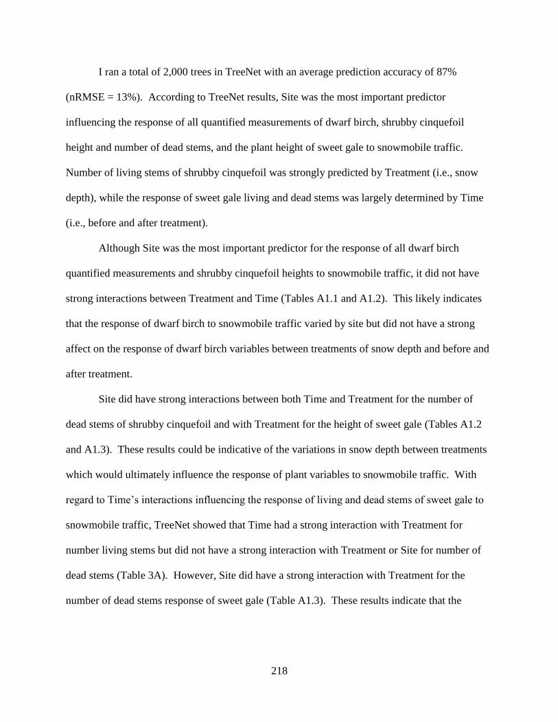
218
I ran a total of 2,000 trees in TreeNet with an average prediction accuracy of 87%
(nRMSE = 13%). According to TreeNet results, Site was the most important predictor
influencing the response of all quantified measurements of dwarf birch, shrubby cinquefoil
height and number of dead stems, and the plant height of sweet gale to snowmobile traffic.
Number of living stems of shrubby cinquefoil was strongly predicted by Treatment (i.e., snow
depth), while the response of sweet gale living and dead stems was largely determined by Time
(i.e., before and after treatment).
Although Site was the most important predictor for the response of all dwarf birch
quantified measurements and shrubby cinquefoil heights to snowmobile traffic, it did not have
strong interactions between Treatment and Time (Tables A1.1 and A1.2). This likely indicates
that the response of dwarf birch to snowmobile traffic varied by site but did not have a strong
affect on the response of dwarf birch variables between treatments of snow depth and before and
after treatment.
Site did have strong interactions between both Time and Treatment for the number of
dead stems of shrubby cinquefoil and with Treatment for the height of sweet gale (Tables A1.2
and A1.3). These results could be indicative of the variations in snow depth between treatments
which would ultimately influence the response of plant variables to snowmobile traffic. With
regard to Time’s interactions influencing the response of living and dead stems of sweet gale to
snowmobile traffic, TreeNet showed that Time had a strong interaction with Treatment for
number living stems but did not have a strong interaction with Treatment or Site for number of
dead stems (Table 3A). However, Site did have a strong interaction with Treatment for the
number of dead stems response of sweet gale (Table A1.3). These results indicate that the

219
response of living tissue of sweet gale to snowmobile traffic is affected both by differences in
time before and after treatment as well as the depth of snow in which the snowmobiles traverse.
Although the calculations of glmm account for the interactions between Time and
Treatment and the variation between individual measurements at Sites and the average for the
population, machine learning provides a more detailed explanation of what variables are
affecting the outcome of glmms. With Site being such an influential factor in these results, it is
expected that the response of plants species would not only vary from wetland to wetland but
also be dependent on the variations of snow depth and intensity of snowmobile traffic on specific
wetlands. However, overall, the results of both the glmm and machine learning indicate that
dwarf birch, shrubby cinquefoil, and sweet gale in general do respond to the compaction of snow
caused by snowmobiles.

220
Table A1.1 – Two-way interaction results of three predictor variables for each quantified
measurement to determine the response of dwarf birch to snowmobile traffic.
Dwarf Birch
Height
Predictor: SITE
Measure1 Measure2 Predictor
22.38 24.96 TREATMENT
21.86 23.33 TIME
Predictor: TREATMENT
Measure1 Measure2 Predictor
22.38 24.96 SITE
15.71 43.01 TIME
Predictor: TIME
Measure1 Measure2 Predictor
21.86 23.33 SITE
15.71 43.01 TREATMENT
Number of Living Stems
Predictor: SITE
Measure1 Measure2 Predictor
33.75 39.78 TIME
31.70 38.74 TREATMENT
Predictor: TIME
Measure1 Measure2 Predictor
33.75 39.78 SITE
19.66 38.41 TREATMENT
Number of Living Stems
Predictor: TREATMENT
Measure1 Measure2 Predictor
31.70 38.74 SITE
19.66 38.41 TIME

221
Table A1.1 – Continued
Dwarf Birch
Number of Dead Stems
Predictor: SITE
Measure1 Measure2 Predictor
27.76 48.90 TREATMENT
25.69 29.73 TIME
Predictor: TREATMENT
Measure1 Measure2 Predictor
27.76 48.90 SITE
21.94 28.93 TIME
Predictor: TIME
Measure1 Measure2 Predictor
25.69 29.73 SITE
21.94 28.93 TREATMENT
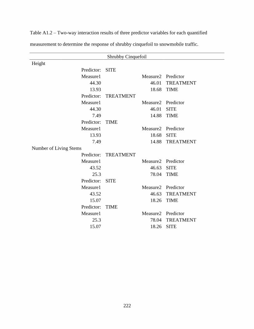
222
Table A1.2 – Two-way interaction results of three predictor variables for each quantified
measurement to determine the response of shrubby cinquefoil to snowmobile traffic.
Shrubby Cinquefoil
Height
Predictor: SITE
Measure1 Measure2 Predictor
44.30 46.01 TREATMENT
13.93 18.68 TIME
Predictor: TREATMENT
Measure1 Measure2 Predictor
44.30 46.01 SITE
7.49 14.88 TIME
Predictor: TIME
Measure1 Measure2 Predictor
13.93 18.68 SITE
7.49 14.88 TREATMENT
Number of Living Stems
Predictor: TREATMENT
Measure1 Measure2 Predictor
43.52 46.63 SITE
25.3 78.04 TIME
Predictor: SITE
Measure1 Measure2 Predictor
43.52 46.63 TREATMENT
15.07 18.26 TIME
Predictor: TIME
Measure1 Measure2 Predictor
25.3 78.04 TREATMENT
15.07 18.26 SITE

223
Table A1.2 - Continued
Shrubby Cinquefoil
Number of Dead Stems
Predictor: SITE
Measure1 Measure2 Predictor
52.59 61.5 TIME
34.93 70.82 TREATMENT
Predictor: TIME
Measure1 Measure2 Predictor
52.59 61.5 SITE
27.43 41.85 TREATMENT
Predictor: TREATMENT
Measure1 Measure2 Predictor
34.93 70.82 SITE
27.43 41.85 TIME

224
Table A1.3 – Two-way interaction results of three predictor variables for each quantified
measurement to determine the response of sweet gale to snowmobile traffic.
Sweet Gale
Height
Predictor: SITE
Measure1 Measure2 Predictor
71.51 73.24 TREATMENT
12.18 26.35 TIME
Predictor: TREATMENT
Measure1 Measure2 Predictor
71.51 73.24 SITE
7.79 14.5 TIME
Predictor: TIME
Measure1 Measure2 Predictor
12.18 26.35 SITE
7.79 14.50 TREATMENT
Number of Living Stems
Predictor: TIME
Measure1 Measure2 Predictor
36.74 42.17 SITE
33.79 75.78 TREATMENT
Predictor: SITE
Measure1 Measure2 Predictor
36.74 42.17 TIME
18.52 23.65 TREATMENT
Predictor: TREATMENT
Measure1 Measure2 Predictor
33.79 75.78 TIME
18.52 23.65 SITE

225
Table A1.3 – Continued
Sweet Gale
Number of Dead Stems
Predictor: SITE
Measure1 Measure2 Predictor
52.59 61.5 TIME
34.93 70.82 TREATMENT
Predictor: TIME
Measure1 Measure2 Predictor
52.59 61.5 SITE
27.43 41.85 TREATMENT
Predictor: TREATMENT
Measure1 Measure2 Predictor
27.41 31.64 TIME
25.34 57.29 SITE

135

227
Appendix 2: Deriving a Spatially Explicit Predictive Model of Snow Depth as a Covariate
in Soundscape and Snowmobile Activity Modeling
To obtain a spatial layer of snow depth for the entire KENWR, I deployed 30 aerial snow
depth markers (i.e., snow benchmarks) throughout KENWR during the summer of 2009. Aerial
snow depth markers are 12 ft tall poles with reflective black and orange horizontal plates placed
12 inches apart. Snow depth is recorded by flying over the snow benchmark and documenting
the lowest visible horizontal bar above the snow.
I determined the spatial distribution of snow benchmarks by overlaying a grid of 15 km2
cells evenly distributed across the Kenai Peninsula. I selected cells with greater than half their
area within the borders of KENWR. I then eliminated cells with more than half their area
consisting of a body of water or glacier. Specific sample sites were chosen for deployment by 1)
identifying a location representing the average elevation of the cell within two standard
deviations and 2) overlaying Digital Orthophoto Quadrangles (DOQs) onto the grid and choosing
sites that were open enough for visual recording from aircraft, had a safe landing area for
helicopter deployment, and were isolated enough to prevent vandalism or collisions with
snowmobilers.
Snow benchmarks were surveyed once a month between December and April for three
winters (2009-2012). Snow depth was estimated to the nearest 0.5 decimeter for all 30 snow
benchmarks where and when possible. In instances when snow benchmarks had either fallen
over or were buried beneath snow, no data were recorded for that site. Those particular snow
benchmarks were re-erected or moved to a new site within the cell the following fall depending
on the circumstance.
228
The latitude and longitude coordinates and the average snow depth for each snow
benchmark were overlaid with spatial layers of elevation, slope, and aspect. These data were
then uploaded into TreeNet machine learning software. To create a spatial map of model
predictions, snow depth-predictor relationships were scored to a regular point grid (500 X 500
m) derived in ArcGIS. These points were also attributed with the same predictor variables to
which the scored predictions could be applied with the appropriate snow depth-predictor
relationship. I then added the scored prediction data to a map of KENWR in ArcGIS. For a
better continuous spatial visualization, the predicted relative index values of each soundscape
component at each point in the grid were then interpolated between neighboring points across the
extent of the study area using the Interpolate-to-Raster and Inverse Distance Weighting (IDW)
tools in ArcGIS Spatial Analyst. This yielded a continuous raster of the predicted distribution of
snow depth in KENWR. The accuracy of our snow depth model was interpreted by calculating
the normalized root mean squared error (nRMSE).
The snow depth model I used for my modeling had an nRMSE = 23%. The order of
importance of predictor variables was elevation, slope, and aspect, respectively. Snow depth was
predicted to be higher at higher elevations, slopes between 7 and 25 degrees, and southeast
aspects.

229
Appendix 3: Identified Sound Sources
Table A3.1 – Table of identified sound sources recorded in the Kenai National Wildlife Refuge
during the winter of 2011-2012.
Biophony Count
Anthrophony Count
Geophony Count
Raven 252
Traffic 3,654
Wind 10,940
Chickadees 114
Airplanes 2,568
Rain 502
Great Horned Owl 85
Snowmobiles 1,583
Running
Water
118
Common Redpoll 42
Compressors 874
Creaking
Branches
27
Red Squirrel 41
Ice Auger 18
4 Sources 11,587
Dark-eyed Junco 33
People Talking 18
Gray Jay 32
Unknown Motor
Noise
12
Boreal Owl 26
Gunshots 11
Woodpeckers 19
Chainsaw 3
Black-billed
Magpie
16
Car Alarm 1
Pine Grosbeak 12
10 Sources 8,742
Goldeneye 8
Ruby-crowned
Kinglet
6
Domestic Dog 5
Ptarmigan 5
Varied Thrush 4
Mallard 4
Bald Eagle 3
Swans 3
Coyote 2
Wolf 1
Wigeon 1
22 Species 714

227

231
Appendix 4: Snowmobile Parking Lot Survey Results
Table A4.1 – Results from a survey of parking lots located at snowmobile trailheads in the
Caribou Hills region conducted for six consecutive Saturdays over winter 2010-2011 and 2011-
2012. Snowmobiles were identified to at least make and to model when possible.
Make Model No. present
Arctic Cat 1M KingCat 1
340 Panther 1
Cougar 3
Crossfire 1
EXT 1
Jag 2
M7 3
M8 1
M1000 2
Powder Special EXT 1
Polaris 550 Sport Touring 1
Classis 1
Indy 5
RMK 30
RXL 1
Short 1
Toury 1
Vertical Edge Trail 1
Vertical Escape 800 1
Vortec 3 1
Ski Doo 380 1
500 1
LE 3
RS 1
Skandic 1
Summit 5
Tundra 3

232
Table A4.1 - Continued
Make Model No. present
Yamaha 550 1
Enticer II 1
Ovation 1
Venture 2
VK550 II 1
Triple 1