TEAM 4 PDR

Kai Jian CheongRichard B. Choroszucha*

Lynn LauMathew MarcucciJasmine Sadler

Sapan ShahChongyu ”Brian” Wang

22.X.2008

Contents

List of Figures . . . . . . . . . . . . . . . . . . . . . . . . . . . . . . . . . . . . . . . . . . . . . . . 3List of Tables . . . . . . . . . . . . . . . . . . . . . . . . . . . . . . . . . . . . . . . . . . . . . . . . 4Abstract . . . . . . . . . . . . . . . . . . . . . . . . . . . . . . . . . . . . . . . . . . . . . . . . . . . 5Executive Summary . . . . . . . . . . . . . . . . . . . . . . . . . . . . . . . . . . . . . . . . . . . . 5

1 Introduction 6

2 Blue Aeroplane Design (FEMA) 72.1 Weight Estimates and Sensitivities . . . . . . . . . . . . . . . . . . . . . . . . . . . . . . . . . 72.2 Wing Loading and Thrust-to-Weight Ratio . . . . . . . . . . . . . . . . . . . . . . . . . . . . 82.3 Aerodynamic Coefficients . . . . . . . . . . . . . . . . . . . . . . . . . . . . . . . . . . . . . . 82.4 Vehicle Performance . . . . . . . . . . . . . . . . . . . . . . . . . . . . . . . . . . . . . . . . . 92.5 Wing Design Characterstics . . . . . . . . . . . . . . . . . . . . . . . . . . . . . . . . . . . . . 102.6 General Fuselage Parameters . . . . . . . . . . . . . . . . . . . . . . . . . . . . . . . . . . . . 102.7 Empennage Placement and Characteristics . . . . . . . . . . . . . . . . . . . . . . . . . . . . 102.8 Landing Gear . . . . . . . . . . . . . . . . . . . . . . . . . . . . . . . . . . . . . . . . . . . . . 112.9 Control Surfaces . . . . . . . . . . . . . . . . . . . . . . . . . . . . . . . . . . . . . . . . . . . 122.10 High Lift System . . . . . . . . . . . . . . . . . . . . . . . . . . . . . . . . . . . . . . . . . . . 122.11 Engine Performance and Placement . . . . . . . . . . . . . . . . . . . . . . . . . . . . . . . . . 132.12 Load Path Layout . . . . . . . . . . . . . . . . . . . . . . . . . . . . . . . . . . . . . . . . . . 142.13 Longitudinal Center of Gravity Position and Excursion . . . . . . . . . . . . . . . . . . . . . . 142.14 Feasibility Study . . . . . . . . . . . . . . . . . . . . . . . . . . . . . . . . . . . . . . . . . . . 14

2.14.1 Tip-Over Analysis . . . . . . . . . . . . . . . . . . . . . . . . . . . . . . . . . . . . . . 142.14.2 Static Margin Analysis . . . . . . . . . . . . . . . . . . . . . . . . . . . . . . . . . . . . 152.14.3 One Engine Inoperative . . . . . . . . . . . . . . . . . . . . . . . . . . . . . . . . . . . 15

2.15 Cost . . . . . . . . . . . . . . . . . . . . . . . . . . . . . . . . . . . . . . . . . . . . . . . . . . 15

3 Red Aeroplane Design (FEMA) 173.1 Weight Estimates and Sensitivity . . . . . . . . . . . . . . . . . . . . . . . . . . . . . . . . . . 173.2 Sizing to Mission Requirements . . . . . . . . . . . . . . . . . . . . . . . . . . . . . . . . . . . 183.3 Aerodynamic Wing Design with a High Lift System . . . . . . . . . . . . . . . . . . . . . . . 183.4 Control Surfaces . . . . . . . . . . . . . . . . . . . . . . . . . . . . . . . . . . . . . . . . . . . 193.5 Aerodynamic Coefficients . . . . . . . . . . . . . . . . . . . . . . . . . . . . . . . . . . . . . . 203.6 Vehicle Performance . . . . . . . . . . . . . . . . . . . . . . . . . . . . . . . . . . . . . . . . . 203.7 Engine Selection and Disposition . . . . . . . . . . . . . . . . . . . . . . . . . . . . . . . . . . 203.8 Fuel System . . . . . . . . . . . . . . . . . . . . . . . . . . . . . . . . . . . . . . . . . . . . . . 203.9 Empennage . . . . . . . . . . . . . . . . . . . . . . . . . . . . . . . . . . . . . . . . . . . . . . 213.10 Landing Gear . . . . . . . . . . . . . . . . . . . . . . . . . . . . . . . . . . . . . . . . . . . . . 213.11 Load Path Layout . . . . . . . . . . . . . . . . . . . . . . . . . . . . . . . . . . . . . . . . . . 223.12 CG Position and Excursion . . . . . . . . . . . . . . . . . . . . . . . . . . . . . . . . . . . . . 233.13 Feasibility Study . . . . . . . . . . . . . . . . . . . . . . . . . . . . . . . . . . . . . . . . . . . 233.14 Cost Estimate . . . . . . . . . . . . . . . . . . . . . . . . . . . . . . . . . . . . . . . . . . . . . 23

1

4 White Aeroplane Design (USAF) 254.1 Weight Estimates and Sensitivities . . . . . . . . . . . . . . . . . . . . . . . . . . . . . . . . . 254.2 Power Loading and Wing Loading . . . . . . . . . . . . . . . . . . . . . . . . . . . . . . . . . 264.3 Aerodynamic Coefficients . . . . . . . . . . . . . . . . . . . . . . . . . . . . . . . . . . . . . . 274.4 Vehicle Performance . . . . . . . . . . . . . . . . . . . . . . . . . . . . . . . . . . . . . . . . . 274.5 Propulsion Selection and Disposition . . . . . . . . . . . . . . . . . . . . . . . . . . . . . . . . 27

4.5.1 Propulsion Selection . . . . . . . . . . . . . . . . . . . . . . . . . . . . . . . . . . . . . 274.5.2 Propulsion Disposition . . . . . . . . . . . . . . . . . . . . . . . . . . . . . . . . . . . . 274.5.3 Fuel System . . . . . . . . . . . . . . . . . . . . . . . . . . . . . . . . . . . . . . . . . . 28

4.6 Wing Aerodynamic Design . . . . . . . . . . . . . . . . . . . . . . . . . . . . . . . . . . . . . 284.6.1 Wing Disposition and Sizing . . . . . . . . . . . . . . . . . . . . . . . . . . . . . . . . 284.6.2 High Lift System . . . . . . . . . . . . . . . . . . . . . . . . . . . . . . . . . . . . . . . 29

4.7 Empennage Aerodynamic Design . . . . . . . . . . . . . . . . . . . . . . . . . . . . . . . . . . 294.8 Landing Gear . . . . . . . . . . . . . . . . . . . . . . . . . . . . . . . . . . . . . . . . . . . . . 304.9 Longitudinal Center of Gravity Position and Excursion . . . . . . . . . . . . . . . . . . . . . . 304.10 Feasibility Studies . . . . . . . . . . . . . . . . . . . . . . . . . . . . . . . . . . . . . . . . . . 31

4.10.1 Static Longitudinal Stability . . . . . . . . . . . . . . . . . . . . . . . . . . . . . . . . 314.10.2 One-Engine-Out Minimum Control Speed . . . . . . . . . . . . . . . . . . . . . . . . . 31

4.11 Cost . . . . . . . . . . . . . . . . . . . . . . . . . . . . . . . . . . . . . . . . . . . . . . . . . . 31

5 Conclusions 33

A Bibliography 35

B Code 37B.1 Blue Aeroplane Code . . . . . . . . . . . . . . . . . . . . . . . . . . . . . . . . . . . . . . . . . 37

B.1.1 Wing Loading Sizing Code . . . . . . . . . . . . . . . . . . . . . . . . . . . . . . . . . 37B.1.2 Professor Powell’s parasiteDragCoeff Code . . . . . . . . . . . . . . . . . . . . . . . . . 38B.1.3 Blue: Static Margin . . . . . . . . . . . . . . . . . . . . . . . . . . . . . . . . . . . . . 38B.1.4 Blue: Weights Estimation . . . . . . . . . . . . . . . . . . . . . . . . . . . . . . . . . . 39B.1.5 Blue: Weight Sensitivity . . . . . . . . . . . . . . . . . . . . . . . . . . . . . . . . . . 40

B.2 White Aeroplane Code . . . . . . . . . . . . . . . . . . . . . . . . . . . . . . . . . . . . . . . . 42B.2.1 Weight and Sensitivity . . . . . . . . . . . . . . . . . . . . . . . . . . . . . . . . . . . . 42B.2.2 Cost . . . . . . . . . . . . . . . . . . . . . . . . . . . . . . . . . . . . . . . . . . . . . . 46

C Dimensioned Drawings 48C.1 Red . . . . . . . . . . . . . . . . . . . . . . . . . . . . . . . . . . . . . . . . . . . . . . . . . . 48C.2 White . . . . . . . . . . . . . . . . . . . . . . . . . . . . . . . . . . . . . . . . . . . . . . . . . 49

2

List of Figures

1.1 FEMA Mission Profile . . . . . . . . . . . . . . . . . . . . . . . . . . . . . . . . . . . . . . . . 6

2.1 Blue Design: Aeroplane . . . . . . . . . . . . . . . . . . . . . . . . . . . . . . . . . . . . . . . 72.2 Blue Design: Basis for T/W and W/S parameters . . . . . . . . . . . . . . . . . . . . . . . . 82.3 Blue Design: Isometric View of T-Tail . . . . . . . . . . . . . . . . . . . . . . . . . . . . . . . 112.4 Blue Design: Top View of Control Surfaces On Aeroplane . . . . . . . . . . . . . . . . . . . . 122.5 Blue Design: Sectional Lift Coefficient According to Normalized Wing Span Location . . . . 132.6 Blue Design: GE CF34-10 turbofan engine . . . . . . . . . . . . . . . . . . . . . . . . . . . . . 142.7 Blue Design: CG Excursion . . . . . . . . . . . . . . . . . . . . . . . . . . . . . . . . . . . . . 15

3.1 Red Design: Aeroplane . . . . . . . . . . . . . . . . . . . . . . . . . . . . . . . . . . . . . . . . 173.2 Red Design: Sizing to Various Conditions . . . . . . . . . . . . . . . . . . . . . . . . . . . . . 193.3 Red Design: Rough Sketch of Fuel Tank Locations . . . . . . . . . . . . . . . . . . . . . . . . 213.4 Red Design: Rough Sketch of Load Path . . . . . . . . . . . . . . . . . . . . . . . . . . . . . 223.5 Red Design: Plot of CG Excursion . . . . . . . . . . . . . . . . . . . . . . . . . . . . . . . . . 233.6 Red Design: Plot of Static Margin . . . . . . . . . . . . . . . . . . . . . . . . . . . . . . . . . 24

4.1 White Design: Aeroplane . . . . . . . . . . . . . . . . . . . . . . . . . . . . . . . . . . . . . . 254.2 White Design: Plot of Power Loading and Wing Loading . . . . . . . . . . . . . . . . . . . . 264.3 White Design: Propulsion System Speed Limits . . . . . . . . . . . . . . . . . . . . . . . . . . 284.4 White Design: Sectional Lift Coefficient According to Normalized Wing Span Location . . . . 294.5 White Design: Plot of CG Excursion . . . . . . . . . . . . . . . . . . . . . . . . . . . . . . . . 31

C.1 Red Design: Dimensioned CAD Drawing . . . . . . . . . . . . . . . . . . . . . . . . . . . . . . 48C.2 White Design Design: Dimensioned CAD Drawing . . . . . . . . . . . . . . . . . . . . . . . . 49

3

List of Tables

2.1 Blue Design: Weight Estimates . . . . . . . . . . . . . . . . . . . . . . . . . . . . . . . . . . . 82.2 Blue Design: Refined Weight Estimates . . . . . . . . . . . . . . . . . . . . . . . . . . . . . . 92.3 Blue Design: Weight Sensitivity Analysis Results . . . . . . . . . . . . . . . . . . . . . . . . . 92.4 Blue Design: Aerodynamic Performance Parameters . . . . . . . . . . . . . . . . . . . . . . . 92.5 Blue Design: Aeroplane Performance Parameters . . . . . . . . . . . . . . . . . . . . . . . . . 102.6 Blue Design: Key Wing Geometry Parameters . . . . . . . . . . . . . . . . . . . . . . . . . . 102.7 Blue Design: Key Fuselage and Aeroplane Parameters . . . . . . . . . . . . . . . . . . . . . . 102.8 Blue Design: Horizontal and Vertical Empennage Characteristics . . . . . . . . . . . . . . . . 112.9 Blue Design: Tire Sizing . . . . . . . . . . . . . . . . . . . . . . . . . . . . . . . . . . . . . . . 122.10 Blue Design: Control Surface Locations . . . . . . . . . . . . . . . . . . . . . . . . . . . . . . 132.11 Blue Design: Landing Gear Location From the Nose . . . . . . . . . . . . . . . . . . . . . . . 152.12 Blue Design: Estimated Cost . . . . . . . . . . . . . . . . . . . . . . . . . . . . . . . . . . . . 162.13 Blue Design: Planned Sale Price . . . . . . . . . . . . . . . . . . . . . . . . . . . . . . . . . . 16

3.1 Red Design: Weight Estimates . . . . . . . . . . . . . . . . . . . . . . . . . . . . . . . . . . . 183.2 Red Design: Detailed Weight Estimates . . . . . . . . . . . . . . . . . . . . . . . . . . . . . . 183.3 Red Design: Sensitivity data . . . . . . . . . . . . . . . . . . . . . . . . . . . . . . . . . . . . 183.4 Red Design: Wing Parameters . . . . . . . . . . . . . . . . . . . . . . . . . . . . . . . . . . . 193.5 Red Design: Lift Device Locations . . . . . . . . . . . . . . . . . . . . . . . . . . . . . . . . . 193.6 Red Design: Control Surface Location . . . . . . . . . . . . . . . . . . . . . . . . . . . . . . . 193.7 Red Design: Aerodynamic Coefficients . . . . . . . . . . . . . . . . . . . . . . . . . . . . . . . 203.8 Red Design: Performance . . . . . . . . . . . . . . . . . . . . . . . . . . . . . . . . . . . . . . 203.9 Red Design: Engine Specifications . . . . . . . . . . . . . . . . . . . . . . . . . . . . . . . . . 203.10 Red Design: Empennage Parameters . . . . . . . . . . . . . . . . . . . . . . . . . . . . . . . . 213.11 Red Design: Tire Dimensions . . . . . . . . . . . . . . . . . . . . . . . . . . . . . . . . . . . . 223.12 Red Design: Landing Gear Location from Nose . . . . . . . . . . . . . . . . . . . . . . . . . . 223.13 Red Design: Estimated Cost . . . . . . . . . . . . . . . . . . . . . . . . . . . . . . . . . . . . . 233.14 Red Design: Planned Sale Price . . . . . . . . . . . . . . . . . . . . . . . . . . . . . . . . . . . 24

4.1 White Design: Weight Estimates . . . . . . . . . . . . . . . . . . . . . . . . . . . . . . . . . . 264.2 White Design: Sensitivity Data . . . . . . . . . . . . . . . . . . . . . . . . . . . . . . . . . . . 264.3 White Design: Parasitic Drag Values for Different Configurations . . . . . . . . . . . . . . . . 274.4 White Design: Performance . . . . . . . . . . . . . . . . . . . . . . . . . . . . . . . . . . . . . 274.5 White Design: CF6-80C2A1 Engine Specifications . . . . . . . . . . . . . . . . . . . . . . . . 284.6 White Design: Wing Specifications . . . . . . . . . . . . . . . . . . . . . . . . . . . . . . . . . 294.7 White Design: Empennage Parameters . . . . . . . . . . . . . . . . . . . . . . . . . . . . . . . 304.8 White Design: Landing Gear Size . . . . . . . . . . . . . . . . . . . . . . . . . . . . . . . . . . 304.9 White Design: Approximate CG Locations of Major Components . . . . . . . . . . . . . . . . 304.10 White Design: Estimated Cost . . . . . . . . . . . . . . . . . . . . . . . . . . . . . . . . . . . 324.11 White Design: Planned Sale Price . . . . . . . . . . . . . . . . . . . . . . . . . . . . . . . . . 32

5.1 Table of Comparisons . . . . . . . . . . . . . . . . . . . . . . . . . . . . . . . . . . . . . . . . 335.2 Comparing to Similar Aircraft . . . . . . . . . . . . . . . . . . . . . . . . . . . . . . . . . . . . 34

4

Abstract

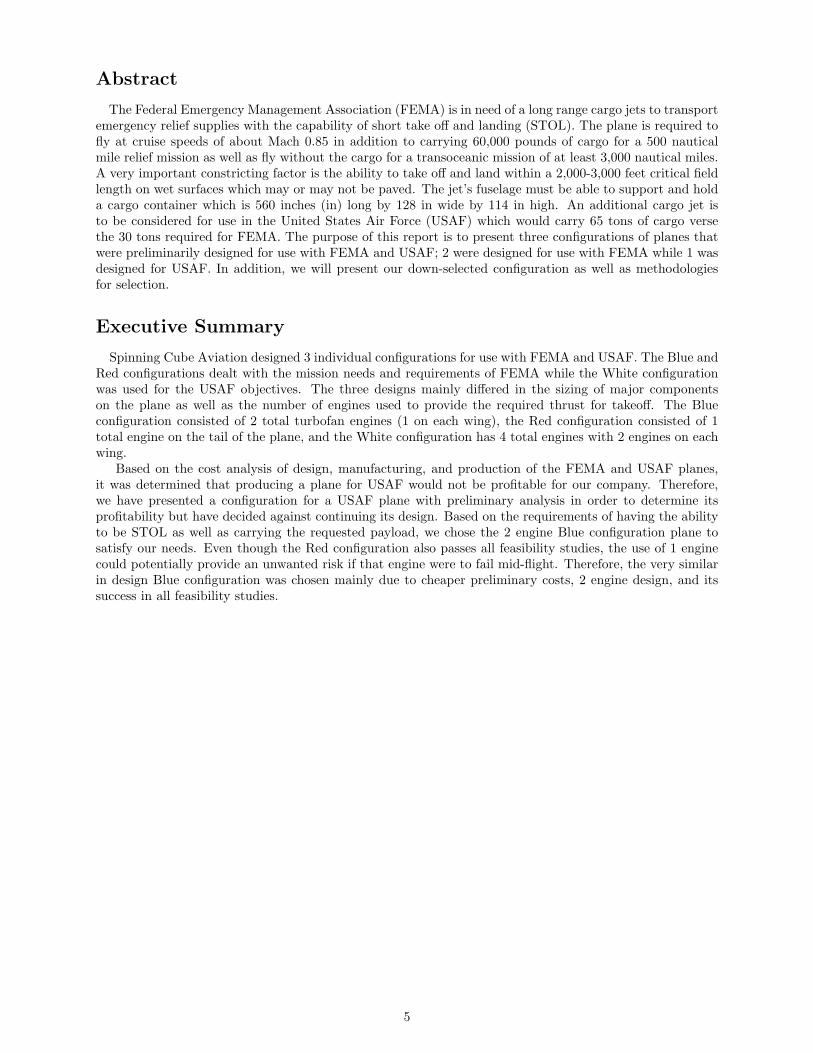
The Federal Emergency Management Association (FEMA) is in need of a long range cargo jets to transportemergency relief supplies with the capability of short take off and landing (STOL). The plane is required tofly at cruise speeds of about Mach 0.85 in addition to carrying 60,000 pounds of cargo for a 500 nauticalmile relief mission as well as fly without the cargo for a transoceanic mission of at least 3,000 nautical miles.A very important constricting factor is the ability to take off and land within a 2,000-3,000 feet critical fieldlength on wet surfaces which may or may not be paved. The jet’s fuselage must be able to support and holda cargo container which is 560 inches (in) long by 128 in wide by 114 in high. An additional cargo jet isto be considered for use in the United States Air Force (USAF) which would carry 65 tons of cargo versethe 30 tons required for FEMA. The purpose of this report is to present three configurations of planes thatwere preliminarily designed for use with FEMA and USAF; 2 were designed for use with FEMA while 1 wasdesigned for USAF. In addition, we will present our down-selected configuration as well as methodologiesfor selection.

Executive Summary

Spinning Cube Aviation designed 3 individual configurations for use with FEMA and USAF. The Blue andRed configurations dealt with the mission needs and requirements of FEMA while the White configurationwas used for the USAF objectives. The three designs mainly differed in the sizing of major componentson the plane as well as the number of engines used to provide the required thrust for takeoff. The Blueconfiguration consisted of 2 total turbofan engines (1 on each wing), the Red configuration consisted of 1total engine on the tail of the plane, and the White configuration has 4 total engines with 2 engines on eachwing.

Based on the cost analysis of design, manufacturing, and production of the FEMA and USAF planes,it was determined that producing a plane for USAF would not be profitable for our company. Therefore,we have presented a configuration for a USAF plane with preliminary analysis in order to determine itsprofitability but have decided against continuing its design. Based on the requirements of having the abilityto be STOL as well as carrying the requested payload, we chose the 2 engine Blue configuration plane tosatisfy our needs. Even though the Red configuration also passes all feasibility studies, the use of 1 enginecould potentially provide an unwanted risk if that engine were to fail mid-flight. Therefore, the very similarin design Blue configuration was chosen mainly due to cheaper preliminary costs, 2 engine design, and itssuccess in all feasibility studies.

5

Chapter 1

Introduction

Spinning Cube has developed three configurations for the FEMA aircraft to perform the relief payloaddelivery and transoceanic ferry mission. They are namely the Red, White and Blue configurations that willbe covered in greater detail later in this report. We arrived at these configurations based on considerationsfor the following parameters and requirements: weight, sizing to mission, wing and empennage design,aerodynamic characteristics, performance aspects, fuel systems, engine selection, landing gear design, loadpath layout, center of gravity excursion, static margin feasibility, tip-over analysis and one-engine-inoperativeanalysis. These subsystems determined the designs we came up with. Of course, we kept to the requirementsgiven for the cruise speed and altitude, as well as the balanced field length and landing zone given.

Our plane was mostly designed around the following mission profile.

Figure 1.1: FEMA Mission Profile

The other mission profiles for a commercial transport can be found in Raymer [4] page 19.

6

Chapter 2

Blue Aeroplane Design (FEMA)

This section of the report discusses the Blue configuration design of the FEMA mission aeroplane. Thecargo plane consists of a high wing structure with 2 General Electric turbofan engines and a T-tail. Theinitial design of the plane was meant to take effective designs from other successful planes while makingmore efficient changes to fulfill the special Short Take Off and Landing (STOL) requirements set forth byFEMA. The Blue configuration can be seen in Figure 2.1 below.

Figure 2.1: Blue Design: Aeroplane

2.1 Weight Estimates and Sensitivities

Preliminary weight estimation was obtained initially by considering historical data of similar types ofplanes, specifically military cargo jets. Using Raymer’s regression data, an approximate weight was obtained.These results are summarized in Table 2.1 below.

This value was used to initially size the different components of the aeroplane. After which a moreaccurate weight analysis was done. This resulted in a gross take-off weight of 253,594 lbs. A detailedbreakdown of the aeroplane’s weight is shown below in Table 2.2.

7

2.2 Wing Loading and Thrust-to-Weight Ratio

Both the wing loading of the aeroplane and its thrust-to-weight (T/W) ratio are strongly dependenton the mission specifications and the certification base (FAR’s). Using methods outlined by Raymer andRoskam, a sizing matching graph was constructed based on individual sizing calculations in order to selectan appropriate wing loading and thrust-to-weight ratio. Individual sizing calculations consisted of sizing theaeroplane to the mission specific take-off, climb, cruise, and landing requirements. A plot of these restrictionson the wing loading and the thrust-to-weight ratio is shown below in Figure 2.2.

Figure 2.2: Blue Design: Basis for T/W and W/S parameters

A high wing loading is desirable in order to reduce the wing size and thus reduce the weight. Low T/Wis advantageous because it also allows for a lower weight due to the use of smaller engines. The sizing plotabove shows a large area where the various requirements are all met; however, choosing a wing loading nearthe maximum allowable value that corresponds to a minimum thrust-to-weight ratio will result in an optimaldesign. Therefore, a wing loading of 72 psf and a thrust-to-weight ratio of 0.37 were chosen to meet thesizing requirements. In this sizing presented, the CLmax for the take-off and landing mission segments wereassumed to be 2.8 and 3.2, respectively. A more detailed explanation of these aerodynamic coefficients isgiven below in § 2.3.

2.3 Aerodynamic Coefficients

Using the data acquired through our weights estimation and wing loading sizing, we were able to obtainan estimation of the maximum coefficient of lift (CLmax

) values at various stages of flight. The values ofCLmax

for take-off, cruise and landing stages are 3, 1.0 and 3.2, respectively. The values for take-off and

Item Weight (lbs)Empty Aircraft 88949Available Fuel 47282Trapped Fuel 1464

Crew 615Payload 60000

Gross Takeoff Weight 198310

Table 2.1: Blue Design: Weight Estimates

8

Item Weight (lbs) Item Weight (lbs)Fuselage 51885 Installed Engines 23311Wing 27540 “All-Else Empty” 31431

Horizontal Tail 6050 Crew 615Vertical Tail 1925 Payload 60000

Front Landing Gear 2385 Trapped Fuel 2427Main Landing Gear 5565 Fuel Available 40459

Gross Takeoff Weight 253594

Table 2.2: Blue Design: Refined Weight Estimates

Parameter varied Abs. Change in WTO (lbs) Relative change in WTO

Payload Weight 2.57 0.84Cruise L/D -2838 -0.25

Range 65.88 0.18Empty Weight 2.09 1.12

Fuel Consumption 69708 0.27Flight Speed -84.6 -0.23

Table 2.3: Blue Design: Weight Sensitivity Analysis Results

landing take into consideration a slat system to increase the CLmaxby about 0.3 and a triple-slated flap on

the main wings to increase the CLmax by about 1.0 past the limits of the supercritical airfoil’s lift.A sensitivity study was also performed in order to better understand which parameters drive the design.

The results of this analysis are shown below in Table 2.3.

Flight Stage Clmaxe Cdo L/D

Take-off 2.8 0.75 0.0352 5.21Cruise 0.173 0.8 0.0152 10.17

Landing 3.2 0.7 0.1902 3.58

Table 2.4: Blue Design: Aerodynamic Performance Parameters

The study shows that empty weight will be one of the most critical parameters to optimize. By doingso, it will be possible to reduce the take-off weight of the aeroplane. Despite the payload weight also havinga significant effect on the take-off weight, little can be done to optimize this value due to the missionrequirements.

2.4 Vehicle Performance

Taking the take-off and landing weight for a particular mission as well as the specific fuel consumption(SFC) we are able to utilize the Breguet Range Equation to determine the range of the FEMA aeroplane tobe 3,563 nmi. Along with the range of the cargo plane, it was important to consider the thrust-to-weightratio of the aeroplane as a function of the wing loading (W/S). In order to obtain a preliminary design curveto determine both T/W and W/S, it was assumed that the flight ceiling be held constant at 30,000 ft aswell as the cruise Mach to be 0.85. Both of these constants fulfill the requirements set forth by FEMA fortransoceanic and relief mission flights. As can be seen in Table 2.5 below, the relatively low value of W/Sprovides the aeroplane with a moderate T/W ratio.

The determination of a T/W and W/S was based on the sizing of the aeroplane at take-off, cruise,landing, and climb. The most restrictive stages in flight were take-off and landing, and they both providedus with the values needed to ensure proper sizing of wings and turbojet engine parameters. Figure 2.2 onpage 8 shows the plot used to find the appropriate value for T/W and W/S based on the most restrictivestage of flight as determined by Roskam’s equations coded in Matlab in Appendix B.1.

9

Range Altitude Take-off T/W Take-off W/S1924 nm 30000 ft 0.369 72 lbs/ft2

Table 2.5: Blue Design: Aeroplane Performance Parameters

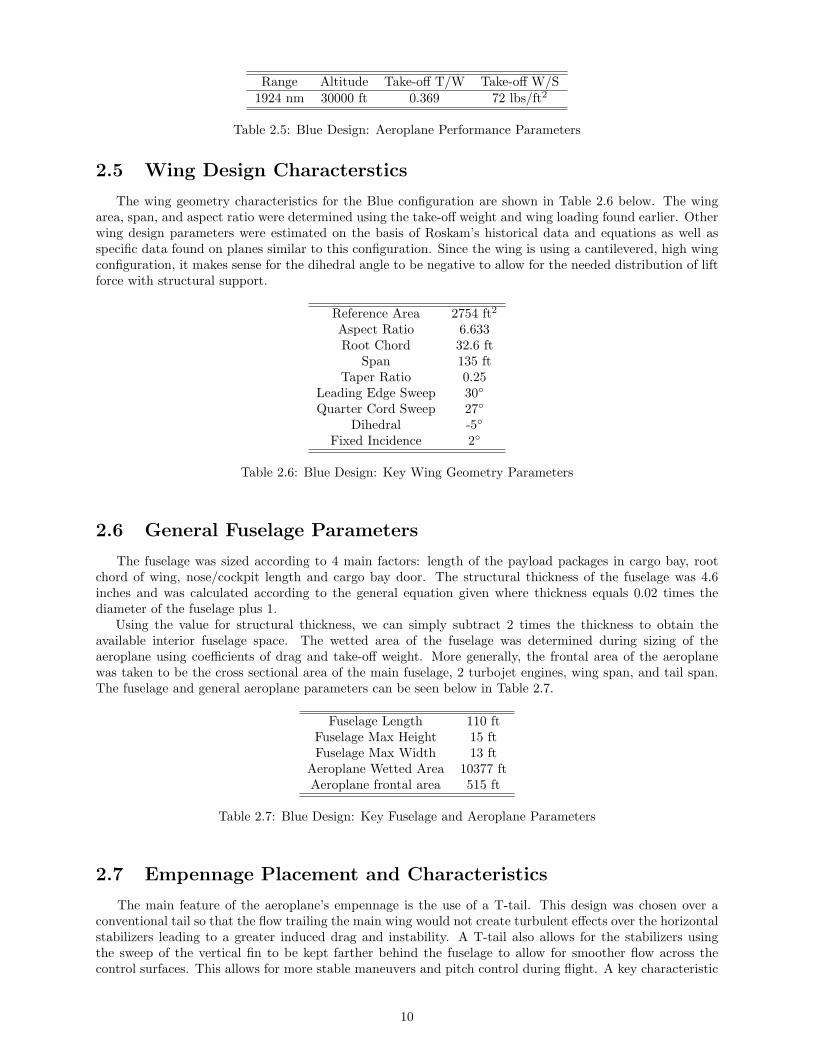
2.5 Wing Design Characterstics

The wing geometry characteristics for the Blue configuration are shown in Table 2.6 below. The wingarea, span, and aspect ratio were determined using the take-off weight and wing loading found earlier. Otherwing design parameters were estimated on the basis of Roskam’s historical data and equations as well asspecific data found on planes similar to this configuration. Since the wing is using a cantilevered, high wingconfiguration, it makes sense for the dihedral angle to be negative to allow for the needed distribution of liftforce with structural support.

Reference Area 2754 ft2

Aspect Ratio 6.633Root Chord 32.6 ft

Span 135 ftTaper Ratio 0.25

Leading Edge Sweep 30◦

Quarter Cord Sweep 27◦

Dihedral -5◦

Fixed Incidence 2◦

Table 2.6: Blue Design: Key Wing Geometry Parameters

2.6 General Fuselage Parameters

The fuselage was sized according to 4 main factors: length of the payload packages in cargo bay, rootchord of wing, nose/cockpit length and cargo bay door. The structural thickness of the fuselage was 4.6inches and was calculated according to the general equation given where thickness equals 0.02 times thediameter of the fuselage plus 1.

Using the value for structural thickness, we can simply subtract 2 times the thickness to obtain theavailable interior fuselage space. The wetted area of the fuselage was determined during sizing of theaeroplane using coefficients of drag and take-off weight. More generally, the frontal area of the aeroplanewas taken to be the cross sectional area of the main fuselage, 2 turbojet engines, wing span, and tail span.The fuselage and general aeroplane parameters can be seen below in Table 2.7.

Fuselage Length 110 ftFuselage Max Height 15 ftFuselage Max Width 13 ft

Aeroplane Wetted Area 10377 ftAeroplane frontal area 515 ft

Table 2.7: Blue Design: Key Fuselage and Aeroplane Parameters

2.7 Empennage Placement and Characteristics

The main feature of the aeroplane’s empennage is the use of a T-tail. This design was chosen over aconventional tail so that the flow trailing the main wing would not create turbulent effects over the horizontalstabilizers leading to a greater induced drag and instability. A T-tail also allows for the stabilizers usingthe sweep of the vertical fin to be kept farther behind the fuselage to allow for smoother flow across thecontrol surfaces. This allows for more stable maneuvers and pitch control during flight. A key characteristic

10

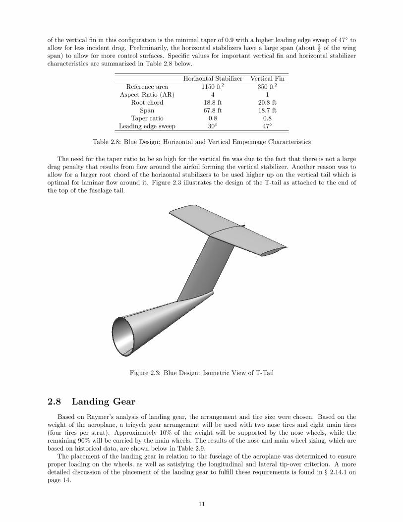
of the vertical fin in this configuration is the minimal taper of 0.9 with a higher leading edge sweep of 47◦ toallow for less incident drag. Preliminarily, the horizontal stabilizers have a large span (about 2

3 of the wingspan) to allow for more control surfaces. Specific values for important vertical fin and horizontal stabilizercharacteristics are summarized in Table 2.8 below.

Horizontal Stabilizer Vertical FinReference area 1150 ft2 350 ft2

Aspect Ratio (AR) 4 1Root chord 18.8 ft 20.8 ft

Span 67.8 ft 18.7 ftTaper ratio 0.8 0.8

Leading edge sweep 30◦ 47◦

Table 2.8: Blue Design: Horizontal and Vertical Empennage Characteristics

The need for the taper ratio to be so high for the vertical fin was due to the fact that there is not a largedrag penalty that results from flow around the airfoil forming the vertical stabilizer. Another reason was toallow for a larger root chord of the horizontal stabilizers to be used higher up on the vertical tail which isoptimal for laminar flow around it. Figure 2.3 illustrates the design of the T-tail as attached to the end ofthe top of the fuselage tail.

Figure 2.3: Blue Design: Isometric View of T-Tail

2.8 Landing Gear

Based on Raymer’s analysis of landing gear, the arrangement and tire size were chosen. Based on theweight of the aeroplane, a tricycle gear arrangement will be used with two nose tires and eight main tires(four tires per strut). Approximately 10% of the weight will be supported by the nose wheels, while theremaining 90% will be carried by the main wheels. The results of the nose and main wheel sizing, which arebased on historical data, are shown below in Table 2.9.

The placement of the landing gear in relation to the fuselage of the aeroplane was determined to ensureproper loading on the wheels, as well as satisfying the longitudinal and lateral tip-over criterion. A moredetailed discussion of the placement of the landing gear to fulfill these requirements is found in § 2.14.1 onpage 14.

11

Diameter (in) Width (in)Nose Wheels 33 12Main Wheels 29 8

Table 2.9: Blue Design: Tire Sizing

2.9 Control Surfaces

Control surfaces of this FEMA mission aeroplane play a vital role in the functionality of the plane in asafe and efficient manner. Due to the unusual take-off and landing terrain as well as possible unsafe weatherconditions, it is highly necessary to implement the most advanced system of control surfaces on the mainwing as well as T-tail. The 5 main surfaces are flaps, slats, ailerons, elevators and rudders. The flaps andslats were discusses previously in the aerodynamic characteristics section while the ailerons, elevators andrudder will be discusses in more detail in this section. In order to understand the benefits and geometricparameters involved with these 3 control surfaces, Figure 2.4 is shown below to illustrate where all surfacesare located in relation to the plane.

Figure 2.4: Blue Design: Top View of Control Surfaces On Aeroplane

The ailerons are placed at what is about the last third of the wing (near the tip) on the trailing edge inorder to allow for more control of the aeroplane’s ability to roll. The pilot is able to operate the aileronsin order to roll for turn or to stabilize the aeroplane back to a natural state after a small disturbance. Thesame idea is applied to the rudder which is attached to the vertical fin on the T-tail. The rudder is usedto control the yaw of the aeroplane so that if a disturbance impacts the aeroplane, the pilot can correct itusing a minor deflection in the rudder to change the horizontal location of the nose. The elevator is locatedon the horizontal stabilizers to allow for more control of the pitch angle of the aeroplane so that the planecan either generate more lift when in need or less when not. The elevators on this configuration will coverclose to 90% of the horizontal stabilizers span. Table 2.10 summarizes the locations of all control surfacesincluding flaps and slats in relation to the inboard and outboard span location and chord fraction.

2.10 High Lift System

The wing requires a high lift system in order to obtain the Cl values given in § 2.3 on page 8 giventhe constraints for a short take and landing (STOL). In the preliminary design stage, the intent is to use aleading edge slat to increase the Cl at a particular angle of attack by about 0.4 and triple-slotted flaps to

12

Flaps Slats Ailerons Elevator RudderInboard span location (normalized) 0.05 0.05 0.6 0.05 0.05

Outboard span location (normalized) 0.6 0.95 0.97 0.9 0.9Inboard chord fraction 0.2 0 0.25 0.25 0.32

Outboard chord fraction 0.2 0.1 0.25 0.25 0.32

Table 2.10: Blue Design: Control Surface Locations

increase the Cl by about 1.9. With these two wing modifications intact, the wing can effectively have anincrease of little under 2.3 above the wing geometry Clmax

. A model of the slat and flap combination on thewing can be seen in Section 2.3 as well.

We were able to determine the location of the flaps along the half span of the wing using a wing loadingcode provided by Professor Powell. After iterations of the code using our wing geometry we were able todetermine the inboard and outboard span-wise location of the trailing edge flaps based on wing stalling atthe particular Cl values. The values of Cl that fall in the shaded box are the only acceptable values to beused because they are the locations where the wing will not stall due to a higher sectional lift to overall liftcoefficient. Figure 2.5 shows the plot used to determine span-wise location of the triple-slotted flaps.

Figure 2.5: Blue Design: Sectional Lift Coefficient According to Normalized Wing Span Location

The leading edge slats are being placed across 90% of the half span wing because there are no othercontrol surfaces placed on the leading edge to interfere with the slats. The slats will allow the aeroplaneto create a higher angle of attack to increase lift without having to actually increase the whole aeroplane’sangle of attack.

2.11 Engine Performance and Placement

In order to power the aircraft based on the iterative estimates for gross takeoff weight and calculated T/Was explained earlier, we chose a 2 engine configuration; 1 turbojet engine on each half-span of the wing. Thetotal required thrust to takeoff is 68,224 lbs, therefore, each engine is only responsible for half that force innormal operable conditions. The General Electric (GE) CF6-6 turbofan engine was chosen because it hada maximum thrust output of 41,500 lbs. This engine provided the closest characteristics to what the Blueconfiguration aircraft needs to operate with a safety cushion of about 6,000 lbs incase of need for extra poweroperation. The engine provides a specific fuel consumption (SFC) of 0.35 lb/(lbf*hour) with a dry weight of8,500 lbs per engine. The diameter is 8.75 ft and the length is 15.67 ft.

13

The placement of the engines will have to be at least 8 ft from the fuselage since the engine diameter is8.75 ft. An estimate of the center point of the engine location along the wing span is 12 ft from the fuselageor .203 inboard half span fraction. The 7.625 ft space between one end of the engine to the main fuselagewill allow for more laminar flow characteristics in that region in order to not create any circulation dueto the colliding flows coming from the engine nacelle and fuselage. Another common feature of the enginelocation is 80% of the engine (inlet to exhaust) will be forward of the leading edge of the wing in order tohelp increase the speed of gas under the wing. Figure 2.6 displays the GE CF34-10 turbofan engine as wellas same key features and dimensions.

Figure 2.6: Blue Design: GE CF34-10 turbofan engine

2.12 Load Path Layout

A load path layout was done for preliminary structural analysis. The layout shows where we expect theappropriate structural supports to carry the specific loads of the aeroplane. As recommended by Raymer fortransport aeroplanes, the fuselage will be constructed with a large number of stringers, which are distributedaround the circumference of the fuselage. Also, necessary structural support was considered on the wingsfor the engines.

2.13 Longitudinal Center of Gravity Position and Excursion

The center of gravity changes as the aeroplane’s overall weight and loading changes. In order to determinehow different scenarios affect the position of the aeroplane’s center of gravity, a CG excursion study wasperformed. Results of this study are in Figure 2.7, below.

The aeroplane’s center of gravity ranges from about 52 to 54 ft from the nose. Thus, the maximumexcursion is approximately 2 ft and corresponds to difference between the aeroplane when it is fully loadedand when it has unloaded the payload, including the appropriate adjustment for fuel burn.

2.14 Feasibility Study

The feasibility of the Blue aeroplane was determined by evaluating the design based on three studies: (1)Tip-Over Analysis, (2) Static Margin Analysis, and (3) One Engine Inoperative. These studies are discussedbelow.

2.14.1 Tip-Over Analysis

The main landing gear must be 15◦ aft of the center of gravity in order to ensure the aeroplane islongitudinally stable. The most aft center of gravity was used to make certain this requirement is fulfilledeven in the most restrictive position. Thus the landing gear must be located at least 4 ft. behind theaeroplane’s center of gravity. The current position of the landing gear places the main wheels about 8 ft.behind the center of gravity, in order to prevent the aeroplane from tipping over. Lateral tip over analysis

14

Figure 2.7: Blue Design: CG Excursion

uses the most forward center of gravity and resulted in approximately 10 ft away from the centerline. Asummary of the landing gear locations are shown in Table 2.11 below.

Nose Gear Location 8 ftMain Gear Location 63 ft, 10 ft away from centerline

Table 2.11: Blue Design: Landing Gear Location From the Nose

2.14.2 Static Margin Analysis

An analysis of the Static Margin was done in order to determine the aircraft’s ability to recover from smalldisturbances in normal flight. Using the method outlined by Raymer resulted in a static margin of 8.8%.This corresponds to the historical data provided by Raymer, which states most transport aircraft have apositive static margin of 5-10%.

2.14.3 One Engine Inoperative

Given the condition that one engine fails, the vertical tail and rudder control surface, for nominaldeflections, must be large enough to compensate for the resulting large yawing moment. The yawing momentthat results from one engine failing is expected to be 591,754 lb-ft. The rudder of the Blue design is capableof providing a counteracting moment of 1,599,600 lb-ft, in order to neutralize the affects of an engine failure.

Therefore, the blue aircraft is considered a feasible design based on the results of the three studies above.

2.15 Cost

A cost estimate of the Blue aeroplane was determined based on the DAPCA IV model, which took intoconsideration the empty weight of the engine, the quantity of aeroplane to be produced and many otherfactors. This estimation is shown below in Table 2.12.

A breakdown of the cost of each plane needed to break even is shown below in Table 2.13. The numberof planes needed to break even corresponds to the number of planes we were asked to produce.

15

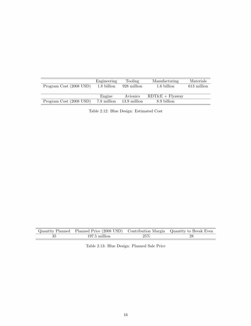
Engineering Tooling Manufacturing MaterialsProgram Cost (2008 USD) 1.8 billion 928 million 1.6 billion 613 million

Engine Avionics RDT&E + FlyawayProgram Cost (2008 USD) 7.8 million 13.9 million 8.9 billion

Table 2.12: Blue Design: Estimated Cost

Quantity Planned Planned Price (2008 USD) Contribution Margin Quantity to Break Even35 197.5 million 25% 28

Table 2.13: Blue Design: Planned Sale Price

16

Chapter 3

Red Aeroplane Design (FEMA)

The Red design is a military cargo category airplane that is designed to carry out the FEMA relief missionwith a maximum payload of 60,000 lbs. It has Short Take-Off and Landing (STOL) field capabilities, andis designed to take off with a balanced field length of 2,500 ft and within a landing field of 3,250 ft. Theaeroplane is powered by a single GE CF6-6 engine that is in a pusher configuration on the tail.

Figure 3.1: Red Design: Aeroplane

3.1 Weight Estimates and Sensitivity

The initial weights estimation reflects the historical statistics of the sizes of the planes that have similarmissions. Using Raymer’s regression data for military cargo planes, we arrived at an approximate weightestimate, as shown in Table 3.1.

The estimate was generated solely based on knowledge from the mission description. As we shaped ourdesign with inclusion of more parts of the aeroplane, we arrived at a more accurate detailed breakdownoutlined in Table 3.2.

Subsequently, we did a quick sensitivity studies to understand what aspects of the airplane affected thetake-off weight significantly.

As we can see from Table 3.3, it will be our empty weight that we have to optimize to reduce the grosstake-off weight.

17

Item Weight (lbs)Empty Aeroplane 136000

Available Fuel 67000Trapped Fuel 4020

Crew 615Payload 60000

Gross Take-off Weight 264000

Table 3.1: Red Design: Weight Estimates

Item Weight (lbs) Item Weight (lbs)Fuselage 25000 Wing 21620

Horizontal Tail 1540 Vertical Tail 913Landing Gear (nose) 1260 Landing Gear (main) 7110

Installed Engines 10600 ’All Else’ 31100Empty Weight 101100Trapped Fuel 1970 Crew 615

Operating Empty Weight 101700Fuel Available 32700 Payload 60000

Gross Take Off Weight 194500

Table 3.2: Red Design: Detailed Weight Estimates

Parameter Varied Abs. Change In WTO (lbs) Rel. Change In WTO

Payload Weight 2.61 0.836Cruise L/D -3730 -0.291

Range 76.9 0.206Empty Weight 2.09 1.12

Fuel Consumption 81300 0.304Flight Speed -98.8 -0.264

Table 3.3: Red Design: Sensitivity data

3.2 Sizing to Mission Requirements

The aeroplane wing loading and thrust to weight ratio are heavily dependent on the mission specifications.Using the mission requirements, we have delineated the limits on our aeroplane design according to take-off,climb, cruise, maneuver, ceiling, stall speed, and landing requirements.

In our design, it will be desirable to reduce wing size and thrust to weight ratio as it will reduce the costof the aeroplane. Thus we need to have high wing loading and low thrust to weight ratio. As such, we havemade assumptions of a CLmax of 3.0 at take-off and landing to achieve a lower thrust to weight ratio. Fromthis sizing, we have picked a wing loading of 76.67 psf and a thrust to weight ratio of 0.3968.

3.3 Aerodynamic Wing Design with a High Lift System

Based on the wing loading chosen from the sizing calculations, the wing reference area is 2162 ft2. Afterfurther deliberations, the following wing parameters were picked.

Most of the decisions were made with reference to Raymer’s suggestions for a large cargo plane, as wellas the mission requirements that drove us to a high wing design. The airfoil NLF(02) - 0215 was chosen forits performance in high Reynold’s number flow, while keeping in mind our cruise Mach number of 0.85.

As shown in the sizing calculations, a high lift system is needed to keep the thrust to weight ratio low.To achieve a CLmax

of 3.0, a triple slotted system with the following location conditions is required.

18

Figure 3.2: Red Design: Sizing to Various Conditions

Wing Parameter ValueReference Area 2162 ft2

Aspect Ratio 9Root Chord 22.1 ft

Span 140 ftTaper Ratio 0.4

Leading Edge Sweep 30◦

Dihedral -3.5◦

Incidence 1◦

Table 3.4: Red Design: Wing Parameters

Flaps SlatsInboard Span Location 0.123 0.123

Outboard Span Location 0.7 1Inboard Chord Location 0.7 0

Outboard Chord Location 1 0.2

Table 3.5: Red Design: Lift Device Locations

3.4 Control Surfaces

The aeroplane needs to have control surfaces that are able to disturb the flow sufficiently to effect a momentto rotate the plane. Inability to do so would mean that the aeroplane may not be controlled. However, atthis point of the design, we can only size the control surfaces according to statistics that Raymer provides.

Ailerons Elevator RudderInboard Span Location (normalized) 0.7 0 0

Outboard Span Location (normalized) 1 1 1Inboard Chord Fraction 0.75 0.75 0.75

Outboard Chord Fraction 1 1 1

Table 3.6: Red Design: Control Surface Location

19

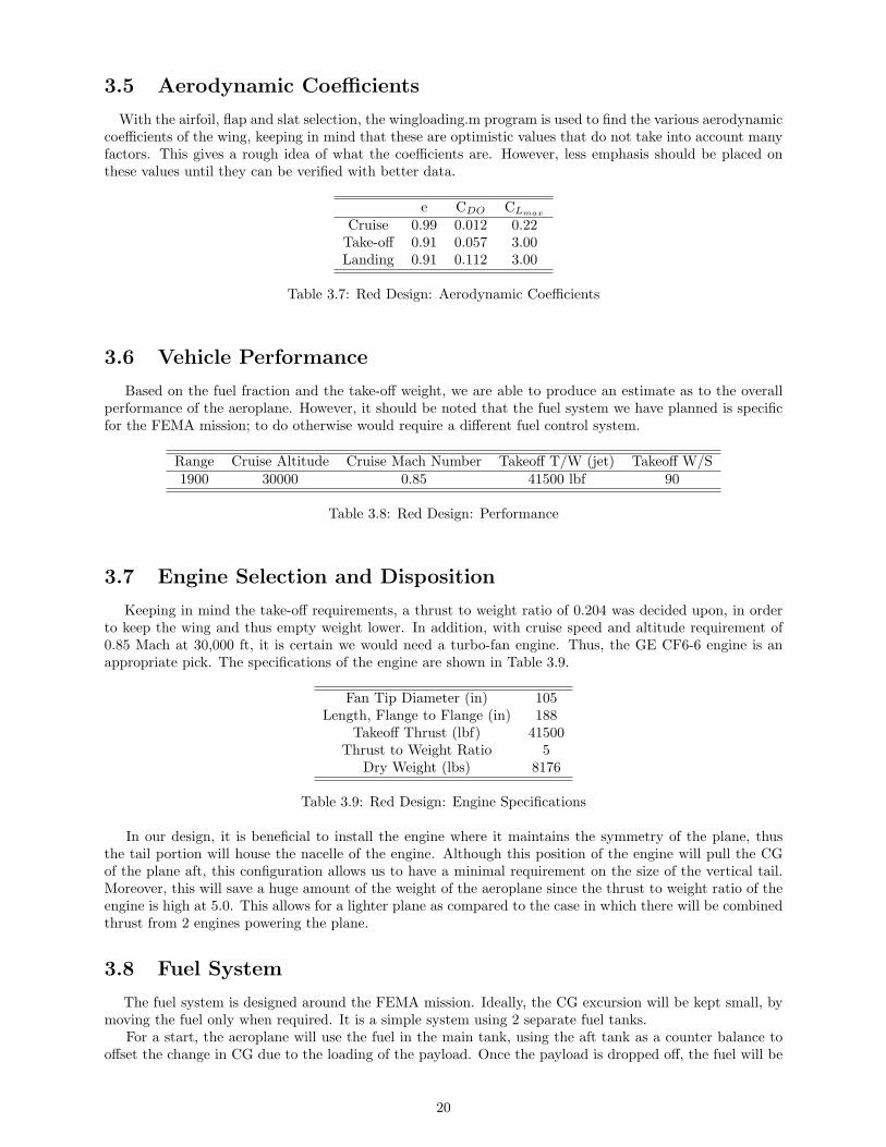
3.5 Aerodynamic Coefficients

With the airfoil, flap and slat selection, the wingloading.m program is used to find the various aerodynamiccoefficients of the wing, keeping in mind that these are optimistic values that do not take into account manyfactors. This gives a rough idea of what the coefficients are. However, less emphasis should be placed onthese values until they can be verified with better data.

e CDO CLmax

Cruise 0.99 0.012 0.22Take-off 0.91 0.057 3.00Landing 0.91 0.112 3.00

Table 3.7: Red Design: Aerodynamic Coefficients

3.6 Vehicle Performance

Based on the fuel fraction and the take-off weight, we are able to produce an estimate as to the overallperformance of the aeroplane. However, it should be noted that the fuel system we have planned is specificfor the FEMA mission; to do otherwise would require a different fuel control system.

Range Cruise Altitude Cruise Mach Number Takeoff T/W (jet) Takeoff W/S1900 30000 0.85 41500 lbf 90

Table 3.8: Red Design: Performance

3.7 Engine Selection and Disposition

Keeping in mind the take-off requirements, a thrust to weight ratio of 0.204 was decided upon, in orderto keep the wing and thus empty weight lower. In addition, with cruise speed and altitude requirement of0.85 Mach at 30,000 ft, it is certain we would need a turbo-fan engine. Thus, the GE CF6-6 engine is anappropriate pick. The specifications of the engine are shown in Table 3.9.

Fan Tip Diameter (in) 105Length, Flange to Flange (in) 188

Takeoff Thrust (lbf) 41500Thrust to Weight Ratio 5

Dry Weight (lbs) 8176

Table 3.9: Red Design: Engine Specifications

In our design, it is beneficial to install the engine where it maintains the symmetry of the plane, thusthe tail portion will house the nacelle of the engine. Although this position of the engine will pull the CGof the plane aft, this configuration allows us to have a minimal requirement on the size of the vertical tail.Moreover, this will save a huge amount of the weight of the aeroplane since the thrust to weight ratio of theengine is high at 5.0. This allows for a lighter plane as compared to the case in which there will be combinedthrust from 2 engines powering the plane.

3.8 Fuel System

The fuel system is designed around the FEMA mission. Ideally, the CG excursion will be kept small, bymoving the fuel only when required. It is a simple system using 2 separate fuel tanks.

For a start, the aeroplane will use the fuel in the main tank, using the aft tank as a counter balance tooffset the change in CG due to the loading of the payload. Once the payload is dropped off, the fuel will be

20

Figure 3.3: Red Design: Rough Sketch of Fuel Tank Locations

pumped from the aft tank to ’refuel’ the main tank, and the engine will once again draw fuel from the maintank.

Fuel is taken from the main tank as the main tank is situated near the CG of the point during bothlegs of the mission. This allows the CG of the plane to stay within tight margins during flight, which isespecially important in keeping the static margin of the plane low while maintaining relative maneuverabilitythroughout the flight.

There are two problems, however, with this design. Firstly, the main tank will intersect with the wingbox. Secondly, the aft tank is placed too close to the engine, which might be hazardous. Should the Redconfiguration be pursued, we will look into changing the position of the engine.

3.9 Empennage

The empennage consists mainly of the horizontal tail and the vertical tail. Due to the size of the wingand the length of the aeroplane, the T-tail design is the most suitable. Also, the tails will be all moving asthis will reduce the size of the tails required.

The sizing of the vertical tail is somewhat removed from statistics as the designed aeroplane is poweredby a single engine, thus removing the restriction on a ’one engine inoperative’ requirement. However, thisrisk means that in the event of a one engine failure during flight, there would be a catastrophic failure of themission.

The sizing of the horizontal tail is based on the sizing of the static margin, which will be discussed to agreater extent later.

The empennage designs are as follows:

Tail Parameters Horizontal Tail Vertical TailReference area (ft2) 279 166

Aspect Ratio 5.6 1.65Root Chord (ft) 10 10

Span (ft) 40 17Taper Ratio 0.4 1

Leading-Edge Sweep (◦) 40 40

Table 3.10: Red Design: Empennage Parameters

3.10 Landing Gear

Our aeroplane will use 2 main gears with 4 wheels each and a 2 wheel nose gear for landing. The landinggears must be able to support the weight of the aeroplane. Once again, using Raymer’s statistical tire sizingdata, we have the tire dimensions.

21

Nose Tire Diameter (ft) 3.9Nose Tire Width (ft) 1.45

Main Tire Diameter (ft) 3.3Main Tire Width (ft) 1.12

Table 3.11: Red Design: Tire Dimensions

However, since both sets of landing gear must ensure the plane is level, there will be a standardized sizefor both sets of tires, taking the larger values. This also has an added advantage of having a standard set ofspare tires.

The location of the landing gears must fulfill both the longitudinal tip-over criterion and the lateral tipover criterion. For a tricycle configuration, the longitudinal tip-over criterion uses the most aft CG locationwhile the lateral tip-over criterion uses the most forward CG location.

Studying both criterions carefully, the location of the landing gears was determined.

Nose Gear location 12 ftMain gear location 57 ft, 10.5 ft away from the centerline

Table 3.12: Red Design: Landing Gear Location from Nose

3.11 Load Path Layout

The load path layout is designed as such to show where we would expect spars to be needed to carry thespecific loads within the aeroplane. The main area of concern is the tail, where we have the tail extendingfrom the nacelle of the engine as it looks like it could be the location of very high stress concentrations.

The landing gears are located at positions where there are readily available support, thus little additionalconsiderations need to be taken for them.

Figure 3.4: Red Design: Rough Sketch of Load Path

22

3.12 CG Position and Excursion

As the airplane progresses in its mission, or even as it is being prepared for a mission, its center of gravitywill move. A study of this to see whether this affects the aeroplane static stability is the CG excursion study.

Figure 3.5: Red Design: Plot of CG Excursion

We can see from Figure 3.5 there is only a point in time when the CG changes significantly, and that iswhen the fuel is adjusted and when the payload is loaded/unloaded. However, this does not affect the staticmargin at all since this process would be done on the ground. This change in CG does affect the tip overanalysis.

3.13 Feasibility Study

Figure 3.6 show how the static margin changes throughout the mission. As described above, only theunloading of payload causes a significant change in the static margin. However, this is offset by the changein CG when we pump the fuel from the aft tank to the main tank before the return flight. Thus we are ableto maintain a static margin of 5% throughout the flight. This is a very acceptable static margin as it meansthat the plane is stable throughout the flight, and is still maneuverable.

3.14 Cost Estimate

In order to ascertain the true feasibility of this design, we need to find an estimate of the cost of theaeroplane. This estimate is based on the empty weight of the engine, the quantity of aeroplane to be producedand many other factors, as stated by the DAPCA IV cost estimate tools that we are using.

Engineering Tooling Manufacturing MaterialsProgram Cost (2008 USD) 1.95 billion 1.03 billion 1.76 billion 0.69 billion

Engine Avionics RDT&E+flyawayProgram Cost (2008 USD) 0.351 billion 0.542 billion 7.8 billion

Table 3.13: Red Design: Estimated Cost

23

Figure 3.6: Red Design: Plot of Static Margin

Finally, we have the calculations for each plane and the number of planes we need to break even. However,the cost calculations are assuming that the goal is to produce the most attractive price to the client, thusthe number of plane we need to sell to break even is set at the number of planes we were asked to produce.

Quantity Planned Planned Price (2008 USD) Contribution Margin Q To Break Even35 223 million 24.2% 35

Table 3.14: Red Design: Planned Sale Price

24

Chapter 4

White Aeroplane Design (USAF)

This design is planned to be used for the United States Air Force. It must meet similar constraints tothose described in the aforementioned sections. In addition, this military aircraft must be able to delivertwo Future Deployable Combat Vehicles. The white team’s design including four turbojet engines, a highcantilevered wing, and a T-tail can be seen below.

Figure 4.1: White Design: Aeroplane

4.1 Weight Estimates and Sensitivities

We used Roskam’s historical data and information given in the mission specifications to calculate theweight of the plane.

Sensitivity is used to see how changing a term (and holding all others constant) would alter other quan-tities. All of the quantities in the chart below will contribute to a change in the take-off weight if they arechanged. This tells us which quantities will be more difficult to change in the long run. The most sensitivedesign driver is the thrust specific fuel consumption. Table 4.2 on page 26 shows the sensitivity data for thevarious parameters.

25

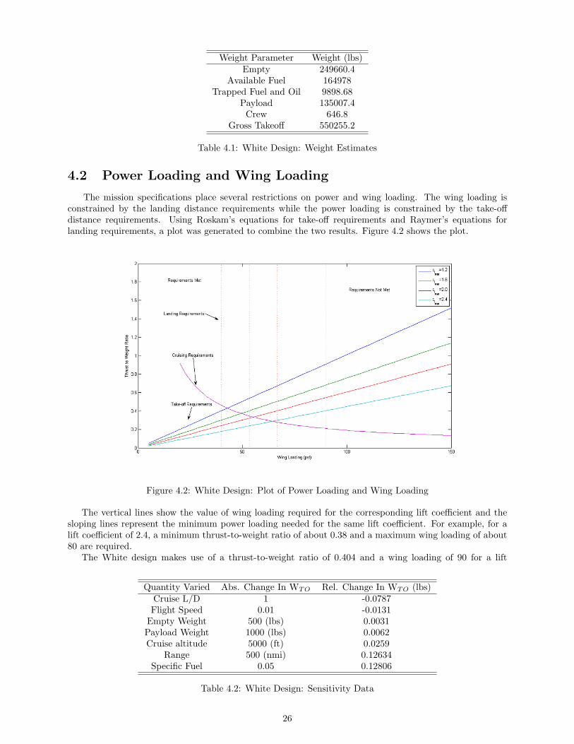
Weight Parameter Weight (lbs)Empty 249660.4

Available Fuel 164978Trapped Fuel and Oil 9898.68

Payload 135007.4Crew 646.8

Gross Takeoff 550255.2

Table 4.1: White Design: Weight Estimates

4.2 Power Loading and Wing Loading

The mission specifications place several restrictions on power and wing loading. The wing loading isconstrained by the landing distance requirements while the power loading is constrained by the take-offdistance requirements. Using Roskam’s equations for take-off requirements and Raymer’s equations forlanding requirements, a plot was generated to combine the two results. Figure 4.2 shows the plot.

Figure 4.2: White Design: Plot of Power Loading and Wing Loading

The vertical lines show the value of wing loading required for the corresponding lift coefficient and thesloping lines represent the minimum power loading needed for the same lift coefficient. For example, for alift coefficient of 2.4, a minimum thrust-to-weight ratio of about 0.38 and a maximum wing loading of about80 are required.

The White design makes use of a thrust-to-weight ratio of 0.404 and a wing loading of 90 for a lift

Quantity Varied Abs. Change In WTO Rel. Change In WTO (lbs)Cruise L/D 1 -0.0787Flight Speed 0.01 -0.0131

Empty Weight 500 (lbs) 0.0031Payload Weight 1000 (lbs) 0.0062Cruise altitude 5000 (ft) 0.0259

Range 500 (nmi) 0.12634Specific Fuel 0.05 0.12806

Table 4.2: White Design: Sensitivity Data

26

coefficient of 2.7. A high lift coefficient is required so as to reduce the wing planform area and the thrustrequired at take-off. This will ensure that the aircraft is able to take-off and land within the distance statedin the mission specifications.

4.3 Aerodynamic Coefficients

Initially, the drag polar must be estimated assuming that drag polar will be parabolic. From the take-offweight, we are able to use Roskam’s equation to calculate the wetted surface area. Then, we can calculatethe equivalent parasitic area. Combining these, the zero-lift (parasite) drag can be calculated. Estimatingan aspect ratio of 6.25 and an Oswald efficiency factor of 0.85 we obtain the following parasite drag fromthe flaps used to take-off and land:

Configuration Drag Polar Equation CLmaxCD

Clean CD=0.0114+0.0599C2L 1.2-1.8 0.09766

Take-off CD=0.0464+0.0634C2L 1.6-2.2 0.3381

Landing CD=0.0939+0.0679C2L 1.8-3.0 0.5889

Table 4.3: White Design: Parasitic Drag Values for Different Configurations

4.4 Vehicle Performance

Using the take-off weight and fuel fractions, a basic vehicle performance can be estimated. Table 4.4shows the vehicle performance parameters.

Range Cruising Mach Take-off Weight T/W W/S5200 nm 0.85 550255.2 lb 0.404 90

Table 4.4: White Design: Performance

4.5 Propulsion Selection and Disposition

The selection of the propulsion system was based on Raymer’s data on suitable propulsion systems relativeto the design Mach number of the aircraft. This data is shown in Figure 4.3. As can be seen, based on ourdesign Mach number of 0.85, a high-bypass turbofan engine is the most suitable system.

4.5.1 Propulsion Selection

The selection of the specific engine was based on calculations of the take-off and landing distancerequirements. Calculations show that a total thrust of 222,303 lbs of thrust is needed for take-off. Thedecision was taken to have four engines instead of two engines because there are limited options for highthrust engines which would be required if only two engines were used. In the event of engine failure, the useof four engines will mean a less drastic loss of thrust.

The use of four engines means that a thrust of about 55,576 lbf is needed per engine. The GeneralElectric CF6-80C2A1 high-bypass turbofan engine was eventually chosen. Table 4.5 on 28 summarizes theengine’s specifications.

4.5.2 Propulsion Disposition

Due to the number of engines chosen and to improve stability, the White design requires the engines tobe mounted under the wing, with two engines on each wing. This will direct the exhaust gases away fromthe primary structures. Since four engines need to be used, they could not be placed on the fuselage. Theroot chord of the fuselage is large enough to support the weight of these four engines.

27

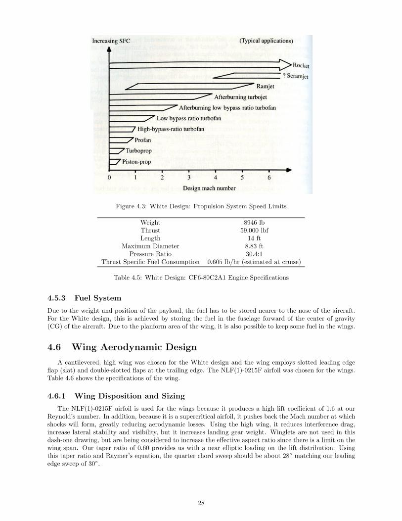
Figure 4.3: White Design: Propulsion System Speed Limits

Weight 8946 lbThrust 59,000 lbfLength 14 ft

Maximum Diameter 8.83 ftPressure Ratio 30.4:1

Thrust Specific Fuel Consumption 0.605 lb/hr (estimated at cruise)

Table 4.5: White Design: CF6-80C2A1 Engine Specifications

4.5.3 Fuel System

Due to the weight and position of the payload, the fuel has to be stored nearer to the nose of the aircraft.For the White design, this is achieved by storing the fuel in the fuselage forward of the center of gravity(CG) of the aircraft. Due to the planform area of the wing, it is also possible to keep some fuel in the wings.

4.6 Wing Aerodynamic Design

A cantilevered, high wing was chosen for the White design and the wing employs slotted leading edgeflap (slat) and double-slotted flaps at the trailing edge. The NLF(1)-0215F airfoil was chosen for the wings.Table 4.6 shows the specifications of the wing.

4.6.1 Wing Disposition and Sizing

The NLF(1)-0215F airfoil is used for the wings because it produces a high lift coefficient of 1.6 at ourReynold’s number. In addition, because it is a supercritical airfoil, it pushes back the Mach number at whichshocks will form, greatly reducing aerodynamic losses. Using the high wing, it reduces interference drag,increase lateral stability and visibility, but it increases landing gear weight. Winglets are not used in thisdash-one drawing, but are being considered to increase the effective aspect ratio since there is a limit on thewing span. Our taper ratio of 0.60 provides us with a near elliptic loading on the lift distribution. Usingthis taper ratio and Raymer’s equation, the quarter chord sweep should be about 28◦ matching our leadingedge sweep of 30◦.

28

Leading Edge Sweep 30◦

Quarter Chord Sweep 28◦

Planform Area 6061.56 ft2

Aspect Ratio 6.25Root Chord 37.88 ft

Span 200 ftTaper Ratio 0.6

Dihedral -3.5◦

MAC Location Chordwise 27.01 ft from LEMAC Location Spanwise 45.83 ft from root chord

Table 4.6: White Design: Wing Specifications

4.6.2 High Lift System

Our target lift coefficient for clean configuration is 1.2 and that for both take-off and landing is 2.7. Bothslats and flaps are used to increase the sectional lift coefficient as well as increase the maximum angle ofattack and thus, stall angle of attack. We made use of Professor Powell’s ’wingLoadingInvisicidFlapped’Matlab code to obtain the maximum lift coefficient possible with our combination of double slotted flapsand slats. The flaps are placed at 20% of the half span and stretch all the way to 70% of the half span.Figure 4.4 shows the sectional lift coefficient of the wing.

Figure 4.4: White Design: Sectional Lift Coefficient According to Normalized Wing Span Location

The results generated from the code showed that the maximum lift coefficient possible is 2.15. This is wellshort of our required lift coefficient of 2.7. In order to address this issue, we are looking into the possibilityof using powered lift such as blown flaps.

4.7 Empennage Aerodynamic Design

We have chosen a T-tail configuration for the empennage of the White Team Design. Although this is aheavier tail, it allows for a smaller vertical tail because of the endplate effect. It will also lift the horizontaltail out of the main-wing wake and propeller wash from the two jet engines (per side). The tail volumecoefficients were taken from historical data and these were used to size the horizontal and vertical tail areas.The taper ratio is also based on historical data. Table 4.7 shows the key empennage parameters.

29

Parameters Horizontal Tail Vertical TailRoot Chord 33.40 ft 41.40 ftTaper Ratio NA 0.8Aspect Ratio NA 1

Planform Area 2345 ft2 1389 ft2

Span 96.85 ft 37.27 ft

Table 4.7: White Design: Empennage Parameters

The White design makes use of the same supercritical airfoil for the tail wings as was used for the mainwings.

4.8 Landing Gear

The landing gear for the White Team Design is quadricycle, retractable, and fuselage-mounted. Thisdesign will have 4 bogeys with 6 wheels each for the main gear struts and the nose gear will consist of twobogeys with 4 wheels each. The position of the struts is determined by adhering to the tip-over criteria forboth longitudinal and lateral.

The main landing gear is located 59.5 ft from the nose and the nose gears are placed at 10 ft from theaircraft nose. As a result of this placement, the angle between the main gear line and the most aft CGposition is 15◦ which meets the longitudinal tip-over requirement. Since the White design uses a quadricycleconfiguration, there is no risk of lateral tip-over.

In order to determine the size of the tires required the static loads on the main and nose landing gearswere calculated. The calculations show that for the main landing gear, a wheel diameter of about 38 in andwidth 13 in are required. For the nose gear, historical data stated that the tires are between 60% and 100%of the main wheels. For the White design, an average value of 80% was used and this resulted in a nosewheel diameter of 35 in and width 12 in. Table 4.8 summarizes these results.

Nose Wheel Diameter Nose Wheel Width Main Dear Diameter Main Gear Width30.71 in 10.28 in 38.39 in 12.85 in

Table 4.8: White Design: Landing Gear Size

4.9 Longitudinal Center of Gravity Position and Excursion

Table 4.9 shows the mass and the approximate CG of the major components of the aircraft. The CGlocations are the longitudinal positions measured from the nose of the aircraft.

Approximate Location (ft)Wing 44.1

Fuselage 59.8Engine 33.2

Horizontal Tail 118.1Vertical Tail 118.1Landing Gear 52.1

”All-else empty” 50.9

Table 4.9: White Design: Approximate CG Locations of Major Components

Summing up the moments of the individual components and dividing by the total mass of the aircraft,we calculated that the most aft CG of the aircraft is located 55.4 ft from the nose of the aircraft. Figure 4.5on page 31 shows the CG excursion of the aircraft. The maximum excursion is calculated to be 3.3ft and thiscorresponds to the scenario where the aircraft is fully fueled and loaded with paratroopers and the payload.

30

Figure 4.5: White Design: Plot of CG Excursion

4.10 Feasibility Studies

Feasibility studies were carried to ascertain if the design parameters are realistic. Two criteria need to bemet in order to satisfy feasibility: static longitudinal stability and one-engine-out minimum control speed.

4.10.1 Static Longitudinal Stability

Stability is determined based on the derivatives of the pitching, yawing and rolling moment coefficients. Aneutral point, which refers to the aircraft aerodynamic center, is calculated and a static margin is established.Static margin is defined as the difference between the neutral point and the aircraft longitudinal CG position,both normalized by the MAC. In order to have static longitudinal stability, a static margin of more than 5%is required.

The neutral point is calculated to be 2.0599MAC and the longitudinal CG position ranges from 2.0527MACto 1.9304MAC. This corresponds to a static margin range of 0.7% to 13%. This clearly fulfills the stabilityrequirement.

4.10.2 One-Engine-Out Minimum Control Speed

A malfunctioning engine will cause changes in the yawing moment. This will come in the form ofmoments due to imbalance in engine thrust as well as moments due to the drag of the stopped engine. Thisis compensated by the size of the vertical tail which has to be large enough to counteract these moments ata minimum control speed.

The yawing moment caused by the sudden malfunction of an engine is calculated to be about 3000kNmand the counteracting moment provided by the deflection of the rudder is calculated to be 1357kNm. Ascan be seen, the counteracting moment provided by the rudder movements is wholly insufficient to overcomethe yawing moment caused by a malfunctioning engine. Thus, the White design does not fulfill this aspectof the feasibility study.

4.11 Cost

The cost estimate of the aircraft is calculated based on the number of aircraft to be produced, theengineering costs, the tooling costs and several other factors as states in DAPCA IV. Tables 4.10 and 4.11summarizes the costs estimates.

31

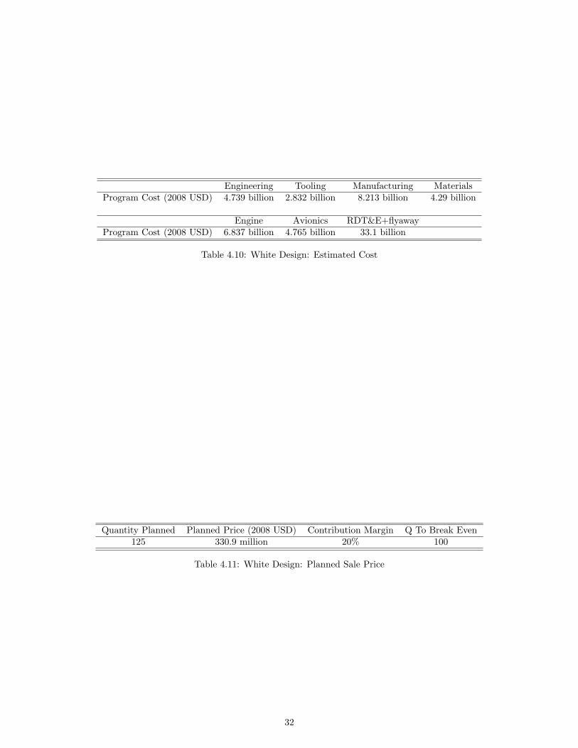
Engineering Tooling Manufacturing MaterialsProgram Cost (2008 USD) 4.739 billion 2.832 billion 8.213 billion 4.29 billion

Engine Avionics RDT&E+flyawayProgram Cost (2008 USD) 6.837 billion 4.765 billion 33.1 billion

Table 4.10: White Design: Estimated Cost

Quantity Planned Planned Price (2008 USD) Contribution Margin Q To Break Even125 330.9 million 20% 100

Table 4.11: White Design: Planned Sale Price

32

Chapter 5

Conclusions

In order to meet FEMA’s need for a long range cargo jet to transport emergency relief supplies with the capa-bility of short take off and landing (STOL), Spinning Cube Aviation developed three different designs(Red,White and Blue), all of which met these basic mission requirements. The White design also considered theUSAF’s need for a new transport plane with similar requirements. An overall comparison between the threedesigns is shown below in Table 5.1.

Blue Red White FinalMission (FEMA or Military) FEMA FEMA Military FEMA

WE (lbs) 99160 88949 249660 88949WTO (lbs) 194462 198310 550255 198310

Cruise Mach number 0.85 0.85 0.85 0.85Price (2008 USD) 223 million 197.5 million 330.9 million 197.5 million

RDT&E + Flyaway Cost (2008 USD) 7.8 billion 8.9 billion 33.1 billion 8.9 billionTakeoff Distance Margin (%) 0.3272 + 4.5% +6% + 4.5%

Landing Distance Margin (% w/% w/o Thrust Rev.) 11%/46% 31% 14%/42% -31%Static Margin (%) 0.07 8.8 0.007 8.8

One-Engine Inoperative Test Passed (Y or N) N/A Y N YTipover Test Passed (Y or N) Y Y Y Y

Table 5.1: Table of Comparisons

The Blue plane was chosen as the final design for continued design work and analysis based on config-uration, cost, and feasibility. The White design did no fulfill the One Engine Inoperative portion of thefeasibility study and thus, was not considered for the final design. Both the Blue and Red designs met all ofthe criteria set by mission requirements and feasibility studies. The Blue design, which utilizes two engines,was chosen based on the higher risk associated with the single engine design used by the White plane. Also,preliminary cost estimations showed the Blue design was less expensive than the Red design. Future workwill focus on developing detailed and feasible aircraft based on the Blue design’s preliminary work. A criticaldesign review is scheduled for early December to review the work completed during this upcoming designphase.

33

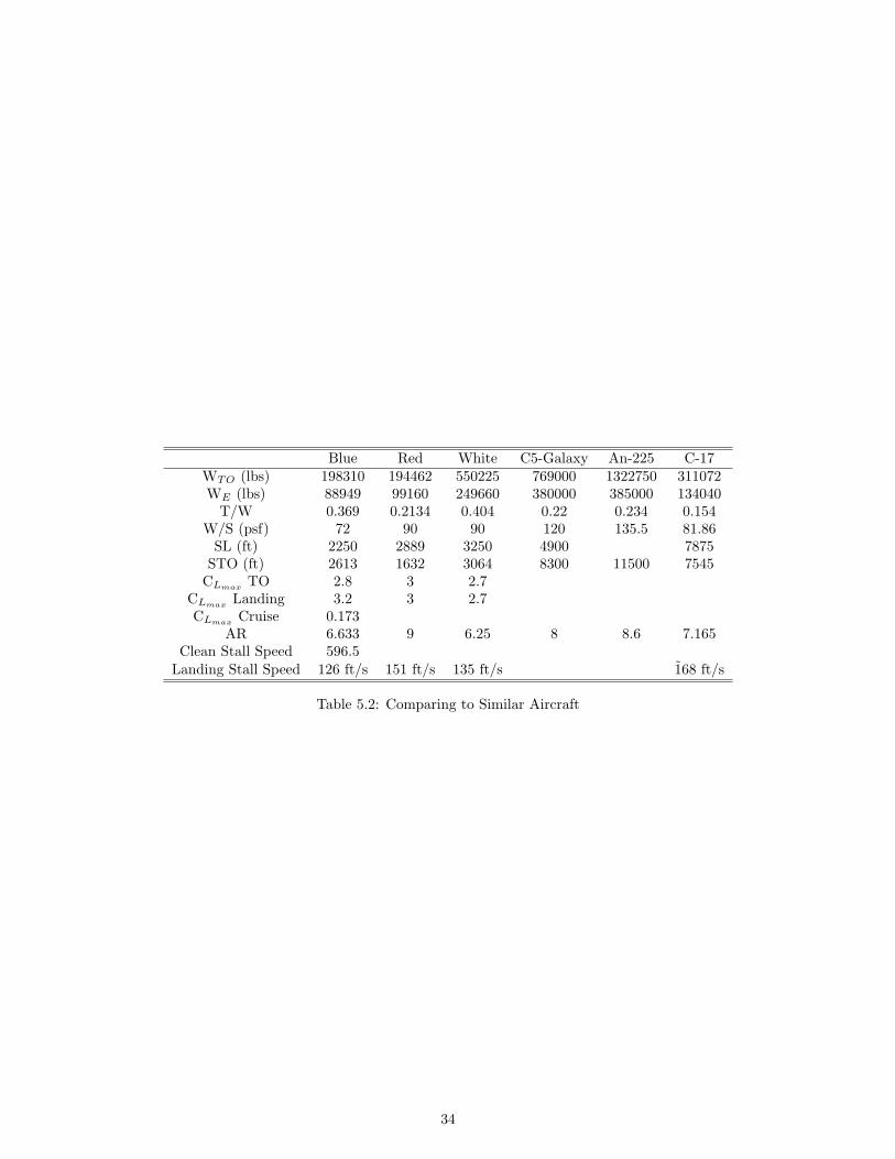
Blue Red White C5-Galaxy An-225 C-17WTO (lbs) 198310 194462 550225 769000 1322750 311072WE (lbs) 88949 99160 249660 380000 385000 134040

T/W 0.369 0.2134 0.404 0.22 0.234 0.154W/S (psf) 72 90 90 120 135.5 81.86

SL (ft) 2250 2889 3250 4900 7875STO (ft) 2613 1632 3064 8300 11500 7545

CLmaxTO 2.8 3 2.7

CLmaxLanding 3.2 3 2.7

CLmax Cruise 0.173AR 6.633 9 6.25 8 8.6 7.165

Clean Stall Speed 596.5Landing Stall Speed 126 ft/s 151 ft/s 135 ft/s 1̃68 ft/s

Table 5.2: Comparing to Similar Aircraft

34

Appendix A

Bibliography

35

Bibliography

[1] “Airlift Cargo Aircraft.” Airlift-Military Aircraft. 19 Nov 1999. Federation of American Scientists. 11Sep 2008. 〈http : //www.fas.org/man/dod − 101/sys/ac/liftcomp.htm〉.

[2] Anderson, John D. Aerodynamics, Fundamentals of. McGraw-Hill. Boston, 2007.

[3] “C-47 Skytrain.” Global Aircraft – C-47 Skytrain. Global Aircraft. 11 Sep 2008〈http : //www.globalaircraft.org/planes/c − 47skytrain.pl〉.

[4] Daniel, P. R. Aircraft Design: A Conceptual Approach 3rd Edition. AIAA Education Series, 1999.

[5] General Electric Company. “GE Aviation Comparison Chart: Turbofans”. 2008. October 13, 2008.〈http : //www.geae.com/engines/commercial/comparisonturbofan.html〉

[6] “KC-97 Stratotanker.” KC-97 Stratotanker-United States Nuclear Forces. 11 Dec 1999. Federation ofAmerican Scientists. 11 Sep 2008 〈http : //www.fas.org/nuke/guide/usa/bomber/kc − 97.htm〉.

[7] Sherman, Robert. “KC-10A Extender.” KC-10A Extender-United States Nu-clear Forces. 10 Mar 1999. Federation of American Scientists. 11 Sep 2008〈http : //www.fas.org/nuke/guide/usa/bomber/kc − 10.htm〉

[8] Philip, H. and Carl, P. Mechanics and Thermodynamics of Propulsion 2nd Edition. Addison-WesleyPublishing Company, 1992

36

Appendix B

Code

B.1 Blue Aeroplane Code

B.1.1 Wing Loading Sizing Code

clear allAR = 6.633*1.2 ; %with winglete_cruise = 0.8;Cdo_cruise = 0.0126;

%Sizing to Take-off requirementTOP = 66.6;CLmax = 3;%this is max take off CLrho1 = 101325/(287*308.15); %air density at landing fieldrho2 = 101325/(287*(273+25)); %air density at normal conditionssigma = rho1/rho2;

WingLoadingD = linspace(0,160);

CLTO=CLmax/1.21;c=-2500;a=0.0149;b=8.134;TOP23=(-b+sqrt(b^2-4*a*c))/(2*a)

Thrust2Weight1 = WingLoadingD/TOP23/sigma/CLTO;hold onplot(WingLoadingD, Thrust2Weight1)xlabel(’Wing Loading (psf)’)ylabel(’Thrust to weight ratio’)

%Sizing to landingCLmaxland = 3.2;Thrust2WeightD = linspace(0,1.3);Wingloading2 = (3250-450)*(sigma*CLmaxland/80)*ones(100);%Wingloading2 = (3250/1.67/0.66-450)/80*sigma*4*ones(100);...%FAR 25 requirement + thrust reversersplot(Wingloading2, Thrust2WeightD)

%Sizing to cruise%altitude - 30000ft or 9144 metersTemp_cruise = (15.04 - 0.00649*9144 + 273.15); %Temperature at cruise (in Kelvins)Press_cruise = 101.29* (Temp_cruise/288.08)^5.256 * 1000; %pressure at cruise in Pa

37

Temp_cruise = Temp_cruise * 1.8; %Temperature at cruise in RankinePress_cruise = Press_cruise * 0.02088545632547; %pressure at cruise in psfV_cruise = 0.85*sqrt(1.4*287*Temp_cruise/1.8)*3.2808399; %cruise speed in ft/sq = 0.5*Press_cruise/1716/Temp_cruise*V_cruise^2; %dynamic pressureWingloading3 = q*sqrt(pi*AR*e_cruise*Cdo_cruise/3)*ones(100);plot(Wingloading3, Thrust2WeightD)

%Sizing to Manuever%consider max load factor to be 2.5n = 2.5;Thrust2Weight4 = (q*Cdo_cruise)./WingLoadingD + n*WingLoadingD/(q*pi*e_cruise*AR);plot(WingLoadingD,Thrust2Weight4)

%Sizing to climb%consider the largest minimum climb gradient of 2.4%Thrust2Weight5 = 0.03+2*sqrt(Cdo_cruise/pi/AR/e_cruise)*ones(100);plot(WingLoadingD, Thrust2Weight5); axis([0 160 0 1]);

B.1.2 Professor Powell’s parasiteDragCoeff Code

%% Military cargo jet parasite drag coefficient calculation%c=0.1628; % From Roskam, for military cargod=0.7316; % From Roskam, for military cargoWTO=184890; % lbs%Swet=10^(c+d*log10(WTO))%cf=0.0030; % From Roskam for jetsf=cf*Swet%wingLoading=90; % psfS=WTO/wingLoadingCD0=f/SAR=6.633;v = 562.25*1.687; %ft/srho = .000889; %lb/ft^3q = 0.5*rho*v^2 %psfe=0.8;G= .29145;ToverW = linspace(.35,1.0,25);WoverS=(((ToverW)-G)+sqrt((ToverW-G).^2-((4*CD0)/(pi*e*AR))))./(2/(q*pi*e*AR));plot(WoverS,ToverW); xlabel(’Wing Load’);ylabel(’Thrust to weight’);...title(’Climb sizing’);

WoverScruise=linspace(0,150,150);ToverWcruise = ((q*CD0)./(WoverScruise)) + (WoverScruise).*(1/(q*pi*e*AR));plot(WoverScruise,ToverWcruise); xlabel(’Wing Load’);ylabel(’Thrust to weight’);...title(’Cruise sizing’); axis([0 150 0 1]);

B.1.3 Blue: Static Margin

clear allWf = 13;Lf = 110;

38

Kf = .05;qhq = 0.9;Dalphah = 0.7;Dcl=6.3;Dclh=6.3;MAC = 26.36;

Xacw = 44/MAC;Xach = 110/MAC;Sw = 2754;Sh = 1150;Dcmfus = (180/pi)*(Kf*Wf^2*Lf)/(MAC*Sw);

xnp = (Dcl * Xacw - Dcmfus + ((qhq)*(Sh/Sw))*Dclh*Dalphah*Xach) .../ (Dcl + ((qhq)*(Sh/Sw))*Dclh*Dalphah)xcg = 53;margin = xnp - (xcg/MAC)

B.1.4 Blue: Weights Estimation

% in FPS unitsclear all%constantsW_per_crew = 175+30;%pounds%inputsM = 0.85;V = 500; %knotsloiter = 0.5;%hoursrange = 500; %nautical miles excluding diversion & descentrangeD = 350;%nautical miles for diversionCrew_num = 3;W_payload = 60000; %lbfW_cargo = 50000;Thrust2Weight = 0.369;WingLoading = 72;e_cruise = 0.8;AR = 6.633*1.2; %with wingletCdo_cruise = 0.0152;Wto1 = 200000;%1st guess

%cruise L/D%altitude - 30000ft or 9144 metersTemp_cruise = (15.04 - 0.00649*9144 + 273.15); %Temperature at cruise (in Kelvins)Press_cruise = 101.29* (Temp_cruise/288.08)^5.256 * 1000; %pressure at cruise in PaTemp_cruise = Temp_cruise * 1.8; %Temperature at cruise in RankinePress_cruise = Press_cruise * 0.02088545632547; %pressure at cruise in psfV_cruise = 0.85*sqrt(1.4*287*Temp_cruise/1.8)*3.2808399; %cruise speed in ft/sq = 0.5*Press_cruise/1716/Temp_cruise*V_cruise^2; %dynamic pressure

Cj_cruise = 0.7; LoD_cruise = 1/( (q*Cdo_cruise/WingLoading)...+(WingLoading/q/pi/AR/e_cruise));%cruise Cj and L/DCj_loiter = 0.5; LoD_loiter = LoD_cruise+1;%loiter Cj and L/D%calculating fuel fractionsff1 = 0.99; %warmupff2 = 0.99; %taxiff3 = 0.995; %take-off

39

ff4 = 1.0065-0.0325*M; %climbff5 = 0.99; %descent; include 100nmff6 = 0.992; %landingffc = exp(-range*Cj_cruise/V/LoD_cruise);%cruise for 500nmffcd = exp(-rangeD*Cj_cruise/V/LoD_cruise);%cruise for 350nmffl = exp(-loiter*Cj_loiter/LoD_loiter);%loiter for 1/2 hour

mff1 = ff1*ff2*ff3*ff4*ff5*ff6*ffc;mff2 = ff4*ff5*ff6*ffcd*ffl/ff6;

%weight iterationW_crew = W_per_crew * Crew_num;A = -0.299; B = 0.8904; %Our regression data for military cargoerr = 10;while err > 1,

Wf1 = Wto1*(1-mff1); %fuel burned in 1st legWb = Wto1-Wf1;%weight after 1st legWa = Wb-W_cargo;%weight after dumping cargoWf2 = Wa*(1-mff1);%fuel burned in 2nd legWf3 = (Wa-Wf2)*(1-mff2);%fuel burned in the diversionWf = 1.06*(Wf1+Wf2+Wf3);%total fuel burned

We = (0.07+(1.71*Wto1^(-0.1))*(AR^0.1)*(Thrust2Weight^0.06)...*(WingLoading^(-0.1))*(M^0.05))*Wto1;...%raymer’s more precise regression for empty weight

Wto2 = W_crew+W_payload+Wf+We;err = abs(Wto2 - Wto1);Wto1 = Wto2;

endWto1WfWe

B.1.5 Blue: Weight Sensitivity

%Weights Sensitivity% in FPS unitsclear all%constantsW_per_crew = 175+30;%pounds%Sensitivity analysisformat long;A = -0.299; B = 0.8904; %Our regression data for military cargo%iteration throughfor i = 0:6

d_pl = 0; dLoD = 0; d_range = 0; d_empty = 0; dCj = 0; dV = 0;if i == 1

d_pl = 1;elseif i == 2

dLoD = 0.01;elseif i == 3

d_range = 1;elseif i == 5

dCj = 0.001;elseif i == 6

dV = 1;end

40

%inputsM = 0.85;V = 500+dV; %knotsloiter = 0.5;%hoursrange = 500+d_range; %nautical miles excluding diversionrangeD = 350;%nautical miles for diversionCrew_num = 3;W_payload = 60000+d_pl; %lbfW_cargo = 50000+d_pl;Thrust2Weight = 0.369;WingLoading = 72;e_cruise = 0.8;AR = 6.633*1.2;Cdo_cruise = 0.0152;

%cruise L/D%altitude - 30000ft or 9144 metersTemp_cruise = (15.04 - 0.00649*9144 + 273.15); %Temperature at cruise (in Kelvins)Press_cruise = 101.29* (Temp_cruise/288.08)^5.256 * 1000; %pressure at cruise in PaTemp_cruise = Temp_cruise * 1.8; %Temperature at cruise in RankinePress_cruise = Press_cruise * 0.02088545632547; %pressure at cruise in psfV_cruise = 0.85*sqrt(1.4*287*Temp_cruise/1.8)*3.2808399; %cruise speed in ft/sq = 0.5*Press_cruise/1716/Temp_cruise*V_cruise^2; %dynamic pressure

Cj_cruise = 0.7+dCj; LoD_cruise = 1/( (q*Cdo_cruise/WingLoading)...+(WingLoading/q/pi/AR/e_cruise))+dLoD;%cruise Cj and L/D

Cj_loiter = 0.5+dCj; LoD_loiter = LoD_cruise+1;%loiter Cj and L/D

%calculating fuel fractionsff1 = 0.99; %warmupff2 = 0.99; %taxiff3 = 0.995; %take-offff4 = 0.98; %climbff5 = 0.99; %descentff6 = 0.992; %landingffc = exp(-range*Cj_cruise/V/LoD_cruise);ffcd = exp(-rangeD*Cj_cruise/V/LoD_cruise);ffl = exp(-loiter*Cj_loiter/LoD_loiter);

mff1 = ff1*ff2*ff3*ff4*ff5*ff6*ffc;mff2 = ff4*ff5*ff6*ffcd*ffl/ff6;

%weight iterationW_crew = W_per_crew * Crew_num;Wto1s = 200000; %lbf - guesserr = 10;while err > 1

Wf1 = Wto1s*(1-mff1); %fuel burned in 1st legWb = Wto1s-Wf1;%weight after 1st legWa = Wb-W_cargo;%weight after dumping cargoWf2 = Wa*(1-mff1);%fuel burned in 2nd legWf3 = (Wa-Wf2)*(1-mff2);%fuel burned in the diversionWf = 1.06*(Wf1+Wf2+Wf3);%total fuel burnedWes = (0.07+(1.71*Wto1s^(-0.1))*(AR^0.1)*(Thrust2Weight^0.06)...*(WingLoading^(-0.1))*(M^0.05))*Wto1s;...%raymer’s more precise regression for empty weightWto2 = (W_payload + W_crew)/(1-(Wf/Wto1s) - (Wes/Wto1s));

41

err = abs(Wto2 - Wto1s);Wto1s = Wto2;

end

if i == 0Wto1 = Wto1s;We = Wes;

end

if i~=0&i~=4%absolute changesD = d_empty+d_pl+dLoD+d_range+dCj+dV;dWto(i) = (Wto1s - Wto1)/D;dWtos = Wto1s-Wto1;%relative changed_pl = d_pl/W_payload;dLoD = dLoD/LoD_cruise;d_range = d_range/range;dCj = dCj/Cj_cruise;dV = dV/V;rc(i) = (dWtos/Wto1)/(d_pl+dLoD+d_range+dCj+dV);end

if i == 4d_empty = 1;Wto3s = (10^((log10(We+d_empty) + A)/B));Wto2s = (10^((log10(We) + A)/B));dWtoe = Wto3s - Wto2s;dWto(i) = dWtoe; d_empty = d_empty/We;rc(i) = (dWtoe/Wto2s)/d_empty;

endenddWto=dWto’rc=rc’

B.2 White Aeroplane Code

B.2.1 Weight and Sensitivity

function weightiter()

%Richard Choroszucha

close all

lb2kg=1/2.2; %Pound to Kilogram

nmi2km=1.852; %Google conversion nmi to km

ft2km=0.0003048; %Conversion feet to kilometers

mPerkm=1000; %Meters Per Kilometer

secsPerHr=3600; %Seconds Per Hour

weold=113482;

wtoold=250116;

dcrew=0; %Person

dwto=0; %lbs

dwe=0;

dcj=0;

dpay=0; %lbs

dfceil=0; %ft

42

dM=0;

dLD=0;

type=’Military’;

fprintf(’\n\n%s\n--------------------------------------------’,type)

crew=3;

wtoguess=(100000*2.2+dwto)*lb2kg;

if (strcmp(’FEMAtrans’,type))

milpass=0;

wpay=(10000+dpay)*lb2kg;

lOverDCruise=(15+dLD)*sqrt(3)/2;

cjCruise=(0.8+dcj); % 1/hr (Roskam)

elseif (strcmp(’FEMArelief’,type))

milpass=0;

wpay=(60000+dpay)*lb2kg;

lOverDCruise=(15+dLD)*sqrt(3)/2;

cjCruise=(0.5+dcj); % 1/hr (Roskam)

elseif (strcmp(’Military’,type))

milpass=25;

wpay=(130000+dpay)*lb2kg;

lOverDCruise=(13+dLD)*sqrt(3)/2;

cjCruise=(0.5+dcj); % 1/hr (Roskam)

end

wcrew=(175+30)*(crew+ceil(dcrew))*lb2kg;

wmilpass=milpass*200*lb2kg;

fceil=(30000+dfceil)*ft2km;

ceiltemp=288.15-6.5*fceil;

R=287;

gamma=1.4;

mCruise=0.85+dM;

aCruise=sqrt(gamma*R*ceiltemp)/mPerkm*secsPerHr; % Speed of Sound at fceil [km/hr]

vCruise=mCruise*aCruise;

mFF=missionfuelfraction(lOverDCruise,mCruise,aCruise,cjCruise,type);

wFBurnedOverWTO=1-mFF;

wFOverWTO=1.06*wFBurnedOverWTO; %25% for loiter and redirect 6% tfo/reserve

fprintf(’\nMission Fuel Fraction for %s mission: %f\n’,type,mFF)

%A=-0.2009; %(Roskam)

%B=1.1037; %(Roskam)

A=0.900847;

B=0.1920292;

error=wtoguess; % lbs, initial guess for gross takeoff weight

n=1;

while(error>1)

%weguess(n)=10^((log10(wtoguess(n))-A)/B); %Original Code

weguess(n)=10^(A*log10(wtoguess(n))+B)+dwe*lb2kg;

wtonew=abs((wpay+wcrew+wmilpass)/(1-wFOverWTO-weguess(n)/wtoguess(n)));

error(n)=abs(wtonew-wtoguess(n));

wtoguess(n+1)=wtonew;

n=n+1;

if (n>1000)

disp(’Too many Iterations. Exiting.’)

break

end

end

figure(1)

plot(1:n,wtoguess,’k’)

xlabel(’Iteration’)

ylabel(’Take-Off Weight’)

title([’Final Take-Off Weight: ’ num2str(wtoguess(n)) ’ [kg]’])

figure(2)

plot(1:(n-1),weguess,’k’)

43

xlabel(’Iteration’)

ylabel(’Empty Weight’)

title([’Final Empty Weight: ’ num2str(weguess(n-1)) ’ [kg]’])

fprintf(’Final Empty Weight: %1.0f [kg] (%1.0f [lbs])\n’,weguess(end),weguess(end)/lb2kg);

fprintf(’Final Take-Off Weight: %1.0f [kg] (%1.0f [lbs])\n’,wtoguess(end),wtoguess(end)/lb2kg)

fprintf(’Final Fuel Weight: %1.0f [kg] (%1.0f [lbs])\n’,wtoguess(end)*wFOverWTO,wtoguess(end)*wFOverWTO/lb2kg)

fprintf(’Final Landing Weight: %1.0f [kg] (%1.0f [lbs])\n’,wtoguess(end)*mFF,wtoguess(end)*mFF/lb2kg)

%sizinggonewrong(weguess(end),wtoguess(end),mCruise,fceil,ceiltemp)

aerocosts(weguess(end),mCruise,aCruise,type)

fprintf(’Relative Change: \n\tW_to: %f \n\tW_e: %f\n’,wtoguess(end)-wtoold,weguess(end)-weold);

%{

figure(3)

plot(1:(n-1),error,’k’)

xlabel(’Iteration’)

ylabel(’Error’)

%}

end

function mff=missionfuelfraction(LD,M,a,Cc,type)

lb2kg=1/2.2; %Pound to Kilogram

nmi2km=1.852; %Google conversion nmi to km

ft2km=0.0003048; %Conversion feet to kilometers

%Cc=22.7; %SFC, LBR Turbofan, SI [m*g/(Ns)]

Cl=0.75*Cc; %SFC, LBR Turbofan, SI [m*g/(Ns)]

LDl=2*sqrt(3)/3*LD;

dr=0;

MClf=0.75; %Climb Mach Factor

redirect=true; %To take into account redirecting

refuel=true; %To take into account refueling at rran

loiter=true; %To take into account loitering.

if (redirect);fprintf(’\nDivert: ON\n’);else fprintf(’Divert: OFF\n’);end

if (refuel);fprintf(’Refuel: ON\n’);else fprintf(’Refuel: OFF\n’);end

if (loiter);fprintf(’Loiter: ON\n’);else fprintf(’Loiter: OFF\n’);end

if (strcmp(type,’FEMAtrans’))

climb=100*nmi2km; %Climb, SI [km]

cran=(3200+dr)*nmi2km; %Cruise Range, SI [km]

rran=1600*nmi2km; %Refuel at, SI [km]

divert=150*nmi2km; %Climb, SI [km]

loitert=0.75; %Loiter Time in Seconds

wi_wi1(1)=0.990*0.990*0.990; %Raymer Warm-up, Taxi and Take-off

wi_wi1(2)=0.980; %Raymer Climb

if (refuel)

R=rran-climb;

wi_wi1(3)=breguet1(R,M*a,Cc,LD)*1.25; %Refuel Point

R=cran-rran-climb;

else

wi_wi1(3)=1; %No refuel

R=cran-climb;

end

wi_wi1(4)=breguet1(R,M*a,Cc,LD); %After Refuel to Descent

if (redirect)

wi_wi1(5)=0.990; %Raymer Descent

wi_wi1(6)=0.992; %Botched Landing

wi_wi1(7)=0.980; %Raymer Climb

R=divert-climb;

wi_wi1(8)=breguet1(R,M*a,Cc,LD); %Redirect

else

wi_wi1(5:7)=1;

wi_wi1(8)=1; %No Diversion, taken into acount in other program

end

44

wi_wi1(9)=sqrt(0.990); %Guess at Descent to Loiter

if (loiter)

wi_wi1(10)=breguet2(loitert,Cl,LDl); %Loiter

else

wi_wi1(10)=1;

end

wi_wi1(11)=sqrt(0.990); %Guess at Loiter to Landing Descent

wi_wi1(12)=0.992; %Raymer Landing

elseif (strcmp(type,’FEMArelief’))

climb=100*nmi2km; %Climb, SI [km]

cran=(500+dr)*nmi2km; %Cruise Range, SI [km]

divert=350*nmi2km; %Climb, SI [km]

loitert=0.5; %Loiter Time in Seconds

wi_wi1(1)=0.990*0.990*0.990; %Raymer Warm-up, Taxi and Take-off

wi_wi1(2)=0.980; %Raymer Climb

R=cran-climb;

wi_wi1(3)=breguet1(R,M*a,Cc,LD); %Cruise to Descent

wi_wi1(4)=0.990; %Raymer Descent

wi_wi1(5)=0.992; %Raymer Landing

wi_wi1(6)=0.990*0.995*0.995*1.05; %Guess at take-off without payload

wi_wi1(7)=0.980; %Raymer Climb

R=cran-climb;

wi_wi1(8)=breguet1(R,M*a,Cc,LD); %After Payload Drop Climb to Descent

if (redirect)

wi_wi1(9)=0.990; %Raymer Descent

wi_wi1(10)=0.980; %Raymer Climb

R=divert-climb;

wi_wi1(11)=breguet1(R,M*a,Cc,LD); %Redirect

else

wi_wi1(9:10)=1;

wi_wi1(11)=1; %No Diversion, taken into acount in other program

end

wi_wi1(12)=sqrt(0.995); %Guess at Descent to Loiter

if (loiter)

wi_wi1(13)=breguet2(loitert,Cl,LDl); %Loiter

else

wi_wi1(13)=1;

end

wi_wi1(14)=sqrt(0.995); %Guess at Loiter to Landing Descent

wi_wi1(15)=0.992; %Raymer Landing

elseif (strcmp(type,’Military’))

climb=100*nmi2km; %Climb, SI [km]

cran=(5000+dr)*nmi2km; %Cruise Range, SI [km]

rran=2500*nmi2km; %Refuel at, SI [km]

divert=200*nmi2km; %Climb, SI [km]

loitert=0.5; %Loiter Time in Seconds

wi_wi1(1)=0.990*0.990*0.990; %Raymer Warm-up, Taxi and Take-off

wi_wi1(2)=0.980; %Raymer Climb

if (refuel)

R=rran-climb;

wi_wi1(3)=breguet1(R,M*a,Cc,LD)*1.25; %Refuel Point

R=cran-rran-climb;

else

wi_wi1(3)=1; %No refuel

R=cran-climb;

end

wi_wi1(4)=breguet1(R,M*a,Cc,LD); %After Refuel to Descent

if (redirect)

wi_wi1(5)=0.990; %Raymer Descent

wi_wi1(6)=0.992; %Botched Landing

wi_wi1(7)=0.980; %Raymer Climb

R=divert-climb;

wi_wi1(8)=breguet1(R,M*a,Cc,LD); %Redirect

else

wi_wi1(5:7)=1;

wi_wi1(8)=1; %No Diversion, taken into acount in other program

end

45

wi_wi1(9)=sqrt(0.990); %Guess at Descent to Loiter

if (loiter)

wi_wi1(10)=breguet2(loitert,Cl,LDl); %Loiter

else

wi_wi1(10)=1;

end

wi_wi1(11)=sqrt(0.990); %Guess at Loiter to Landing Descent

wi_wi1(12)=0.992; %Raymer Landing

else

fprintf(’Error: No Mission Profile Named: %s \nSetting mff=1.0.\n’,type)

end

fprintf(’\nWi/Wi-1:\n’)

for n=1:length(wi_wi1)

fprintf(’Mission Segment: %02.f Fuel Fraction: %0.6f\n’,n,wi_wi1(n))

end

mff=prod(wi_wi1);

%mff=0.7;

function ww=breguet1(R,V,C,LD)

ww=exp(-R*C/(V*LD));

end

function ww=breguet2(E,C,LD)

ww=exp(-E*C/(LD));

end

end

B.2.2 Cost

function aerocosts(We,M,a,type)

nmi2km=1.852;

lb2kN=4.44822162/1000;

irate=[2.19 3.38 2.83 1.59 2.27 2.68 3.39 3.24 2.85]/100;

inffact=1;

for n=1:length(irate)

inffact=inffact*(1+irate(n));

end

inffact;

RE=86;

RT=88;

RQ=81;

RM=73;

V=M*a;

if (strcmp(type,’Military’))

numeng=5;

Q=125;

FTA=2;

Tmax=70000*lb2kN;

Tturb=1628;

else

numeng=4;

Q=35;

FTA=2;

Tmax=53500*lb2kN;

Tturb=1628;

end

HE=5.18*We^0.777*V^0.894*Q^0.163;

HT=7.22*We^0.777*V^0.696*Q^0.263;

HM=10.5*We^0.82*V^0.484*Q^0.641;

HQ=0.076*HM;

46

CD=48.7*We^0.630*V^1.3;

CF=1408*We^0.325*V^0.822*FTA^1.21;

CM=22.6*We^0.921*V^0.621*Q^0.799;

Ceng=2251*(9.66*Tmax+243.25*M+1.74*Tturb-2228);

Cavi=6000*0.02*We*2.2*Q;

Tco=HE*RE+HT*RT+HM*RM+HQ*RQ+CD+CF+CM+Ceng*numeng*Q+Cavi;

(0.8*HE*RE+0.2*HQ*RQ+0.6*CD+CF)*inffact;

b=1E0;

fprintf(’\nEngineering Cost: USD2008$%1.0f (USD1999$%1.0f)\n’,HE*RE*inffact/b,HE*RE/b)

fprintf(’Tooling Cost: USD2008$%1.0f (USD1999$%1.0f)\n’,HT*RT*inffact/b,HT*RT/b)

fprintf(’Manufacturing Cost USD2008$%1.0f (USD1999$%1.0f)\n’,HM*RM*inffact/b,HM*RM/b)

fprintf(’Materials Cost: USD2008$%1.0f (USD1999$%1.0f)\n’,CM*inffact/b,CM/b)

fprintf(’Engine Cost: USD2008$%1.0f (USD1999$%1.0f)\n’,Ceng*inffact*numeng*Q/b,Ceng*numeng*Q/b)

fprintf(’Avionics Cost: USD2008$%1.0f (USD1999$%1.0f)\n’,Cavi*inffact/b,Cavi/b)

fprintf(’RD&T and Flyaway Cost: USD2008$%1.0f (USD1999$%1.0f)\n’,Tco*inffact/b,Tco/b)

fprintf(’Cost Per Plane: USD2008$%1.0f (USD1999$%1.0f)\n’,Tco*inffact/Q,Tco/Q)

47

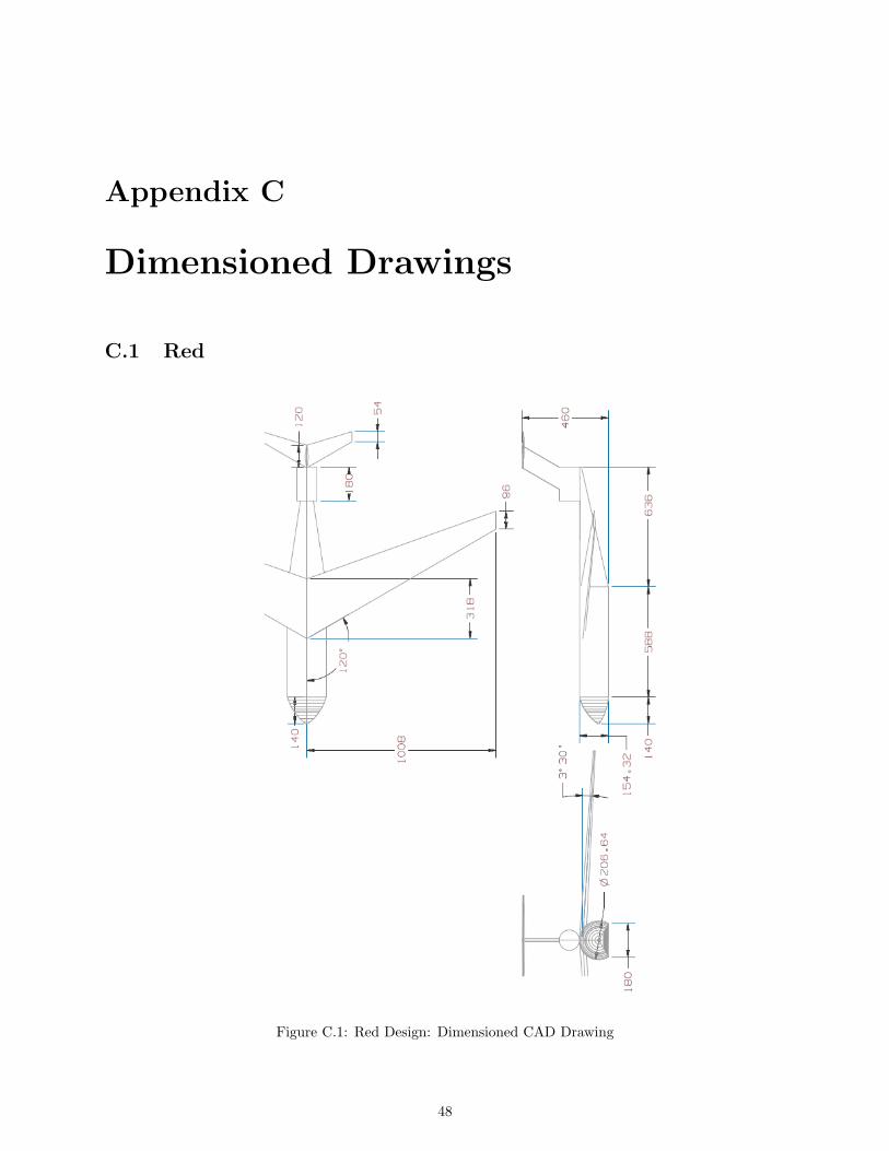
Appendix C

Dimensioned Drawings

C.1 Red

Figure C.1: Red Design: Dimensioned CAD Drawing

48

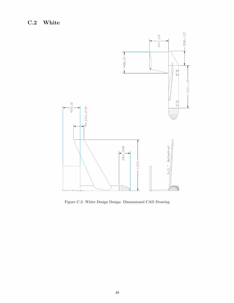
C.2 White

Figure C.2: White Design Design: Dimensioned CAD Drawing

49