Team Incentives under Private Contracting∗

Korok Ray

Texas A&M University

Monday 28th November, 2016

Abstract

I model a moral hazard in teams problem in which the principal offers private

contracts. Public contracts are common knowledge to all agents, but private con-

tracts are known only between the principal and each individual agent. Public

contracts can induce efficient outcomes, but are subject to collusion between the

principal and any given agent. Private contracts by construction are immune to

this collusion and generate contracts that are subject to a budget balance con-

straint. Thus, the budget balance constraint emerges endogenously, whereas most

team incentive problems take this constraint as given.

∗I’d like to thank Cindy Alexander, Richard Hanus, Heber Farnsworth, Pierre Liang, Jack Stecher,

Qintao Fan, and seminar participants at the SEC and the 2016 Management Accounting Section meet-

ing. Texas A&M provided generous financial and research support.

1 Introduction

There’s no question that teamwork is vital to modern organizations, as teams perme-

ate all levels of the corporate hierarchy (boards, executive teams, partnerships, project

teams). Much of the prior literature has modeled these teams as a collection of agents

who receive individual or joint contracts on their output. Yet an underlying assumption

is that the contracts are public, namely, that all team members know the contracts of-

fered to the others. In practice, contracts are largely private, and agents rarely know

the full details offered to other members of the team.1 I explore the economic effects

on teamwork of private contracts and find the surprising result that private contracts in

equilibrium will satisfy budget balance, a constraint that the literature on team incen-

tives has long taken as given.

Public contracting is the benchmark case that has occupied most of the prior liter-

ature on team production. The principal simultaneously makes offers that are public

(known to all parties); this gives rise to the bonding contract of Holmstrom (1982), in

which every agent becomes a residual claimant on the firm’s output, and the principal

charges each agent the efficient output level up front. Though this achieves efficiency,

one chief problem of this bonding contract is that the principal has an incentive to re-

duce output, even though he captures total surplus. He effectively pays more than $1

in wages for every dollar in output, and therefore has an incentive to strike a private

contract with any one agent to reduce effort. This private contract would be amenable

to both parties; the agent is held to his reservation utility anyway, and the principal

gains if output falls. The possibility of private contracts breaks the bonding contract.

This begs the question of what the equilibrium looks like under full private contract-

ing. I propose a model of private contracts, in which the principal makes contracts to a

team of agents, but each agent only knows of their own contract. Each agent therefore

must speculate on the contract given to other agents. As the contract that any agent

sees could be a signal of the contracts offered to other agents, this creates a complex

signaling game of multiple equilibria. To narrow the scope of the problem, I follow

1For example, a private conversation with a retired Big Four audit partner has revealed that Ernst

& Young currently uses a “closed” system, in which each partnership share is not disclosed across

partners (private contract). At one point, Arthur Andersen had an “open” system (public contract),

but now most of the Big Four auditors keep their partner distributions secret. And for good reason, as

compensation can be a sensitive topic that reveals performance, which both the firm and the partner

may prefer to keep between each other, not announced to all parties.

2

the literature to consider only passive beliefs: if the principal deviates from an agent’s

equilibrium contract, that agent believes that all other agents continue to face their

equilibrium contracts.

Under this assumption, the participation constraint for each agent now changes,

since each agent only knows of his own contract. The main result shows that under a

certain class of production functions (additive separability in each agents’ effort choice),

every equilibrium in the private contracting game will satisfy budget balance, classically

defined over the team of productive agents (not including the principal). In this sense,

the ability to privately contract generates the budget balance constraint endogenously,

which the large literature on team incentives takes as given.

The intuition behind this result fundamentally stems from externalities. Under team

production, since payment is made on group output there is a positive externality from

any agent’s effort choice on other agents. Once any given agent has already committed

to exert his efficient effort, he creates a positive externality on the second agent, who

implicitly has already received some benefit from the first agent’s work. At that point,

the principal and second agent are both better off if the second agent shirks. Private

contracts can thus break the public contracting equilibrium. Ultimately, the principal’s

payoff function is invariant to changes in output if and only if budget balance holds

exactly. In that case, the principal will have no incentives to privately contract to

either increase or decrease any individual agent’s effort. The additive separability on

production ensures that there are no interaction effects between different agents that

would lead to further private contracts. This is fundamentally why budget balance

emerges in equilibrium under private contracting and separable production.

In this sense, the literature has come full circle. The initial literature assumed budget

balance as an exogenous constraint imposed on team production because it resembled a

feature observed in some specific teams (like partnerships). But the constraint has real

economic content, as apparent through the private contracting game. Budget balance

kills the principal’s incentives to privately contract because it makes its payoff function

insensitive to changes in output.

Surprisingly, the emergence of budget balance can still occur even in a more general

model of complementarity in production. General complementarity will introduce inter-

action effects between the different agents. Normalizing the complementarity factor to

one, I show that budget balance holds in every equilibrium of the bilateral contracting

game, even when the effort of different team members are perfect complements rather

3

than perfect substitutes. This provides some modicum of reassurance that the results

are not limited to a narrow class of production functions.

Much of the literature splits between team production (Holmstrom (1982), Huddart

and Liang (2005), Legros and Matsushima (1991), Legros and Matthews (1993), Miller

(1997), and Rasmusen (1987)) and cost sharing or cost allocation (Rajan (1992), Ray

and Goldmanis (2012), and Baldenius et al. (2007)). The two problems are formally

equivalent. Segal (1999), Segal and Whinston (2003), and McAfee and Schwartz (1994)

establish some of the early framework for bilateral contracting, in particular the role of

externalities. Segal and Whinston (2003) address private contracts in procurement and

in inter-firm relationships, but not in the specific framework relevant for this paper.

I do not consider private contracts between the agents themselves, as Holmstrom and

Milgrom (1990), Macho-Stadler and Perez-Castrillo (1993), Ramakrishnan and Thakor

(1991), Itoh (1993), and Varian (1990). Those papers all require some kind of individual

performance measure, or the ability for agents to observe action choices of other agents

that the principal cannot, which does not fit the setting of this paper. But more im-

portantly, the temptation to privately contract rests with the principal, not with each

individual agent. Even though the principal captures total surplus at the efficient effort

profile, he still has the temptation to reduce aggregate output. It is this temptation that

leads to privately contracting with any individual agent in order to reduce output.

The literature on repeated games has relevance for my results as well, such as Abreu

et al (1993). For example, Baker et al (1994) show that implicit incentives can serve

as a complement to explicit incentives in a repeated game between a single principal

and single agent. Che and Yoo (2001) show that the optimal incentive scheme uses

low powered group incentives in a repeated game with a principal and a team. Both

of these papers, like much of the repeated game literature, lean on the repetition of

a static game to sustain equilibria that would vanish in a one shot game, using folk

theorem style arguments. While I do not consider repeated games here, the notion of

private contracting conceptually takes place in a dynamic setting. Indeed, the broad

literature on repeated games in contract theory provides additional context for the more

traditional explicit incentives considered here. Future research will provide more explicit

characterizations of this dynamic interaction, and it will illustrate more explicitly how

the possibility of building a reputation may make available equilibria that were previously

unavailable in a one shot game.

4

2 The Model

Consider a risk-neutral principal contracting with n risk-neutral agents. Each agent i

exerts effort ei ≥ 0 at cost Ci(ei), where C ′i > 0, C ′′

i > 0 and Ci(0) = 0. Let N = {1..n}be the team and let e ≡ (ei)i∈N be the effort vector of all agents. Let q : Rn

+ → R+

be the team production function.2 Each agent observes only his own effort, while all

parties (principal and all agents) observe joint output q = q(e). Let qi(e) ≡ ∂q(e)∂ei

> 0, and∂2q(e)∂e2i

≤ 0. Thus the team production function exhibits diminishing marginal returns and

is increasing. Furthermore, I remain agnostic on the cross partial∂qij(e)

∂ei∂ej, which could be

positive, zero, or even negative. A positive cross-partial would indicate complementarity

between agents, while a zero cross-partial would imply that their efforts are perfect

substitutes.

The first best allocation e∗ maximizes total surplus:

e∗ ∈ argmaxe

q(e)−∑

i

Ci(ei), (1)

yielding qi(e∗) = C ′

i(e∗i ). The marginal cost of effort equals its marginal return, given

by the marginal productivity of any given agent’s effort on team production. First best

output is q∗ ≡ q(e∗).

2.1 Public Contracting

A bilateral contract is a salary and bonus (si, bi) for agent i where

wi = wi(q) = si + biq (2)

is agent i’s wage. I restrict attention to wages that are linear in output in order to gain

traction on the sharing rules bi of joint output q. Moreover, this fits many common

applications in practice, in which partnerships receive a fixed salary (possibly negative,

to allow a buy-in to the partnership). I do not impose limited liability on the contract,

though in equilibrium the bonus terms will be positive. McAfee and MacMillan (1991)

show that linear contracts on joint output are optimal in a model of moral hazard and

2There is no measurement error in output. Because joint output is pooled across agents, there is

inherent difficulty in measuring the performance of each agent, even if output is measured without noise.

Because agents are risk-neutral, adding a noise term is straightforward and simply involves replacing q

with Eq throughout the paper. To ease analysis, I omit the noise term.

5

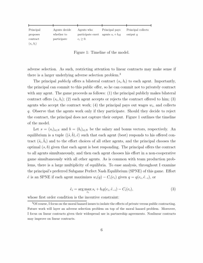
Principal

proposes

contract

(si, bi)

Agents decide

whether to

participate

Agents who

participate exert

ei ≥ 0.

Principal pays

agents si + biq

Principal collects

output q

Figure 1: Timeline of the model.

adverse selection. As such, restricting attention to linear contracts may make sense if

there is a larger underlying adverse selection problem.3

The principal publicly offers a bilateral contract (si, bi) to each agent. Importantly,

the principal can commit to this public offer, so he can commit not to privately contract

with any agent. The game proceeds as follows: (1) the principal publicly makes bilateral

contract offers (si, bi); (2) each agent accepts or rejects the contract offered to him; (3)

agents who accept the contract work; (4) the principal pays out wages wi, and collects

q. Observe that the agents work only if they participate. Should they decide to reject

the contract, the principal does not capture their output. Figure 1 outlines the timeline

of the model.

Let s = (si)i∈N and b = (bi)i∈N be the salary and bonus vectors, respectively. An

equilibrium is a tuple 〈(s, b), e〉 such that each agent (best) responds to his offered con-

tract (si, bi) and to the effort choices of all other agents, and the principal chooses the

optimal (s, b) given that each agent is best responding. The principal offers the contract

to all agents simultaneously, and then each agent chooses his effort in a non-cooperative

game simultaneously with all other agents. As is common with team production prob-

lems, there is a large multiplicity of equilibria. To ease analysis, throughout I examine

the principal’s preferred Subgame Perfect Nash Equilibrium (SPNE) of this game. Effort

e is an SPNE if each agent maximizes wi(q)− Ci(ei) given q = q(ei, e−i), or

ei = argmaxei

si + biq(ei, e−i)− Ci(ei), (3)

whose first order condition is the incentive constraint:

3Of course, I focus on the moral hazard issues to isolate the effects of private versus public contracting.

Future work will layer an adverse selection problem on top of the moral hazard problem. Moreover,

I focus on linear contracts given their widespread use in partnership agreements. Nonlinear contracts

may improve on linear contracts.

6

biqi(e) = C ′i(ei) (IC)

Observe the second order conditions hold by assumption:

bi∂qi(e)

∂ei− C ′′

i (ei) < 0. (SOSC)

Note that a bonus vector b = (bi)i∈N induces an effort vector e(b), so the principal’s

optimal b induces an optimal effort vector e ≡ e(b). Call a contract (s, b) an equilibrium

contract if 〈(s, b), e(b)〉 is an equilibrium.

Each agent has an outside option, normalized to zero. The principal can always

offer each agent their outside option of si = bi = 0, so ei = 0. It is without loss of

generality to restrict attention to equilibria in which all agents participate. Each agent

will participate if he gets nonnegative utility in equilibrium, or wi − Ci(ei) ≥ 0:

si + biq ≥ Ci(ei) (PCi)

The principal will select each si such that (PCi) binds. As usual, this occurs because

the salary only transfers rent between the principal and each agent, but does not affect

the incentive constraint. The principal will substitute the binding (PCi) into her payoffs

π = q −∑i wi so:

b ∈ argmaxb

q(e(b))−∑

i

Ci(ei(b)). (4)

The principal’s profit function is identical to total surplus, and therefore the principal

can implement efficient effort by choosing bi = b∗i = 1, so ei = e∗i . From binding (PC),

optimal salary is

s∗i = Ci(e∗i)− q∗ < 0, (5)

since total surplus = q∗ −∑i Ci(e∗i) > 0. Thus, the principal can implement the first

best under public contracts. This is the standard bonding contract, where the principal

compensates each agent for his individual cost of effort, and each agent pays q∗ up front.

The principal makes each agent the residual claimant to guarantee efficient labor supply.

Since the agents are held to their participation constraints, the principal earns all the

7

rents, so the principal’s profit is π∗ > 0.4 Every agent faces a negative salary,5 similar

to the feature of many professional partnerships that require partners to buy into the

partnership, such as in accounting, law, or medicine. Moreover, the large tournaments

literature pioneered by Lazear and Rosen (1979) use these bonding contracts: the agents

are risk neutral, the win/loss prizes are large, and the principal collects the surplus from

the agents through a bonding fee upfront.

The principal acts as an independent party who shares in the output of the team

but bears no cost of production. As Holmstrom (1982) noted, introducing such a third

party achieves efficiency even under “budget balance.” Of course, the budget is bal-

anced in a trivial sense, because the third party plays no role in production, and any

choice of sharing rules would balance the budget because the third party acts as a sink

(Miller 1997).6 See Rasmusen (1987) for further analysis of the sink, such as the use of

scapegoat and massacre contracts. A scapegoat contract punishes a single agent if the

team deviates, and a massacre contract punishes all if a team deviates. Rasmusen (1987)

examines team production under risk aversion, where such extreme contracts are welfare-

enhancing. However, this is not relevant for this setting because of the risk neutrality

of the agents. Both of these scapegoat and massacre contracts are nonlinear solutions

that implement first best. They are multi-agent versions of the classic forcing contract

in which the principal pays a prize if the agent achieves first best output, but nothing

otherwise. These contracts, however, face criticism since they require full commitment

from the principal. The principal will need to know the solution it seeks to induce and

commit to levying harsh penalties if output varies from that solution. I focus on linear

contracts for their wide practical use as well as lower commitment requirements.

Every agent earns the full return to their labor but pays for this through a large

negative salary. In practice, limited liability constraints of agents will prohibit the use

4Note that the principal could easily break even by raising the salaries si to the point that π = 0.

This passes the surplus from the principal to the agents, but does not change incentives. This would

still be a SPNE. However, the principal prefers the SPNE in which she takes all the rents, and the

agents are held to their reservation utilities.5If agents faced a general outside option u > 0, the efficient salary would be u + Ci(e

∗

i ) − q∗. This

salary could be positive for high enough outside options because the salary is a linear increasing function

of u. These outside options do not change the bonus contract, so the contract overall is qualitatively

unchanged, making the normalization of u = 0 without loss of generality.6To see that the budget is balanced, let wp = q −∑iwi be the principal’s wage. Then the sum of

all wages is trivially equal to output: wp +∑

iwi = q.

8

of large negative salaries. But this is not the only problem with the efficient contract,

as it leads to collusion between the principal and agent.

3 Private Contracting

In many contracting scenarios (such as employment), the principal contracts privately

with each agent, even when the agents work together on a joint project. If the principal

cannot commit to public contracts, but instead can make private contracts with each

agent, the equilibrium contract above can no longer implement the first best effort

allocation. To see this, consider a simple example.

Example: Let n = 2. Let output be q(e1, e2) = e1+e2. Let Ci(ei) =12e2i , so C

′i(ei) = ei.

First best effort is e∗i = 1, first best output is q∗ = 2, and cost of effort is C(e∗i ) =12.

Total surplus is q∗ −∑Ci(e∗i ) = 1. The efficient bonus that implements first best is

b∗i = 1 with a salary of s∗i = 12− 2 = −3

2. Each agent earns u∗

i = 0. The principal’s

profit is π∗ = q∗(1−∑ b∗i )−∑

s∗i = 1. Suppose that both agents agree to this contract.

However, after signing the contract but before working, the principal makes a private

contract with the second agent. He renegotiates by proposing a new contract (s2, b2)

where s2 = b2 = 0. Facing this contract, the agent will select effort e2 = 0 earning utility

u2 = 0, making him indifferent between this new contract and his original one. If he

accepts the new private contract, then the principal pays for output only from the first

agent, so his profit is

π = e∗1 − b∗1e∗1 − s∗1 =

3

2> 1 = π∗ . (6)

�

In the example, the principal has an incentive to privately contract with one agent

in order to reduce his output. Even in this simple example of perfect substitutes and

identical agents, the principal is better off by reducing the second agent’s effort to 0.

Indeed, this logic is general, and such private contracts break the equilibrium under

public offers. More generally, the equilibrium under public contracts is no longer stable

under private contracting:

9

Proposition 1 If the principal cannot commit to public offers, then b∗i = 1 is never an

equilibrium. As a result, the first-best is not implementable.

The principal is strictly better off by privately contracting with agent k to shirk.

Intuitively, if the principal sets bi = 1 for each i, she pays n dollars in wages for every

dollar of output, so she has an incentive to privately contract with one agent to reduce

his effort, yielding output q < q∗. She earns less revenue, but she also saves Ck(e∗k) from

not employing agent k, and (q∗− q) on each of the n− 1 workers who do work. The net

benefit is positive if n ≥ 2. Once I replace the public offers with private contracts, the

original equilibrium is no longer stable. There are many other possible private contracts

in this new game that break the equilibrium (s, b) in the original public offers game

above.7

Proposition 1 complements Eswaran and Kotwal (1984), who find that if the principal

cannot commit to public offers, group penalty schemes cannot implement first-best effort

in a moral hazard in teams setup. Group penalty schemes are nonlinear forcing contracts,

paying out bonuses to all agents only if all agents select first-best effort. My result gives

a similar impossibility in the world of linear contracts on joint output. Both results rely

on private contracting to break the public contracting equilibrium.

The extreme punishment contracts, such as the scapegoat and massacre contracts,

will still suffer from the same effects of private contracting as the standard efficient

bonding contract. In particular, these extreme punishment contracts can induce any

effort level, say, e∗. Because of this, if the principal could privately contract with any

other agent, he would do so after all other agents have committed to e∗−i. The principal

still has an incentive to reduce output for any agent. In other words, the extreme

punishment contracts are not subgame perfect in the private contracting game.

3.1 Budget Balance

It turns out that there is a very close link, proven later, between private contracting and

budget balance, the condition that the bonus coefficients across all agents sum to one.

7More generally, suppose the principal offers agent k an additional payment sk to reduce output to

some q < q∗. Before, the principal earned π∗ = q∗ −∑iw∗

i = q∗ −∑i(si + biq∗) = q∗(1 − n) −∑i si,

whereas now she earns π = q(1−n)−∑i si−sk. The principal gains if π > π∗, or if sk < (q−q∗)(n−1).

The agent will agree if w∗

k = si + q∗ < wk = si + q + sk, or if sk > (q∗ − q) > 0. Hence, both parties

accept this new contract if sk ∈ (q∗ − q, (q∗ − q)(n− 1)).

10

Definition 1 A bonus vector b satisfies Budget Balance (BB) if∑

bi = 1.

This is a common and well known feature of most team incentive problems. It shows

up in both team production as well as in the cost allocation literature.8 Both of these

literatures usually take budget balance as an exogenous constraint on the contracting

problem. They largely defend the assumption on intuitive grounds, such as a cost

allocation rule that is “tidy” as in Demski (1981).

Consider the bilateral surplus between the principal and some agent k:

BSk(e) = q −∑

i

wi + wk − Ck(ek) = q(e)−∑

i 6=k

wi(q(e))− Ck(ek). (7)

Bilateral surplus is unlike total surplus because it does include some transfers. Recall

that total surplus is a sum of all payoffs, both from the set of productive agents, as well

as from the principal who collects output. As such, transfers between agents fall out of

the surplus function. Since bilateral surplus only considers the joint utility of a principal

and one agent, wages of all other agents will remain inside the surplus function. This is

the summation on the right hand side of the equation above.

Definition 2 Call a contract (s, b) bilaterally efficient if

ek ∈ argmaxek

BSk(ek, e−k) (8)

for each k, where e = e(b) is the effort generated by b.

In words, each agent’s effort is generated by a bilaterally efficient contract that

maximizes the bilateral surplus between the agent and the principal, holding all other

agents to their contractually generated effort levels.

Corollary 1 If (s, b) is bilaterally efficient, then budget balance holds.

Corollary 1 shows that maximizing bilateral surplus yields a budget balancing con-

tract. Indeed, the bilateral surplus is simply joint output less the wages of all other

agents, less the cost of effort of agent k. However, when maximizing bilateral surplus,

8Specifically, Moulin (2008), Moulin and Shenker (1992), and Ray and Goldmanis (2012) impose

budget balance in a cost allocation problem, and Huddart and Liang (2005), Legros and Matsushima

(1991), Legros and Matthews (1993), and Miller (1997) impose budget balance in a partnership setting.

11

the firm can substitute in the incentive constraint for agent k, which includes that agent’s

bonus. Thus, the wage payments include the bonus of all other agents plus the bonus

for agent k, which itself is the bonus of the entire team.

This must balance perfectly the coefficient on team output, which is one. This

intuitively expresses why budget balance must hold. The proof of Corollary 1 provides a

direct proof, but a simple argument provides the intuition. If the budget balance failed,

then the sum of the bonuses may exceed or fall short of unity. Thus, there would be one

agent k who would have a bonus strictly greater than or less than one. If the former,

the principal would have an incentive to sign a contract with that agent to decrease

his bonus, causing him to reduce effort and the principal to save on costly incentive

payments. If the latter, the principal would have an incentive to sign a contract with

that agent to increase his bonus, which would elicit more effort out of him and generate

higher joint output. This would violate the initial claim that the original contract was

bilaterally efficient, since the principal and agent k would now be better off.

To fix ideas, consider output functions that are additively separable, in which output

is a linear combination of the effort of each agent.

Definition 3 Output q(e) is additively separable if q(e) =∑n

i=1 αiei.

Now, αi represents the differential contribution of each agent to the team’s output.

Observe that αi and effort are complements, so αi is a productivity parameter for agent

i. High αi agents enjoy a higher return from their labor. To focus the analysis on moral

hazard, I do not assume αi to be private information but rather common knowledge to

all participants.

It turns out that budget balance and separability determine the optimal bonuses.

Proposition 2 Suppose q is additively separable and costs are quadratic (so Ci(ei) =ci2e2i for ci > 0). If a contract maximizes total surplus subject to budget balance, then the

unique bonus is given by:

bi = 1−ciα2

i

1n−1

∑i

ciαi

2

. (9)

As shown earlier, maximizing total surplus alone gives the unique contract of b∗i = 1,

which generates efficiency. Imposing budget balance constrains the bonuses to∑

bi = 1,

and their optimal level is given in the proposition. It is easy to verify that budget

balance holds for (9).

12

3.2 General Analysis

The principal offers the contract (si, bi) to each agent privately, so agents cannot observe

each other’s contracts. Each agent’s decision to participate now depends on his beliefs

about offers extended to the other agents. When the agent receives an offer from the

principal he must speculate on the offers made to other agents. As such, the initial

offer to agent i may serve as a signal on the offers to other agents. While arbitrary

beliefs on out-of-equilibrium offers can generate many Perfect Bayesian equilibria, I

will follow Segal (1999) and McAfee and Schwartz (1994) by restricting attention to

“passive beliefs”: after observing an (out-of-equilibrium) offer from the principal, an

agent believes that the other agents continue to face their equilibrium offers. Call this

game the private contracting game. The timeline of the private contracting game is

identical to the public contracting game, as the only difference is the observability of

the contracts.

Suppose b is the equilibrium bonus vector, generating equilibrium effort e = e(b).

If the principal offers bi to agent i, then the agent will accept the contract if he earns

nonnegative utility, given that all other agents still choose their equilibrium effort e−i.

The principal can always default to no trade and hold each agent to si = bi = 0.

Therefore the participation constraint is now

si + biq(ei, e−i) ≥ Ci(ei) (PC ′i)

This (PC ′i) differs from (PCi) in that the other agents’ effort is held fixed at the

equilibrium levels. This matters because the principal will substitute the participation

constraint into the objective function, and whether e−i is held at its equilibrium level or

not will alter the principal’s objective function. This is the only operational difference

between public and private contracting. The rest of the problem (such as the incentive

constraint) remains the same. Also, (PC ′i) is a more restrictive condition than the

participation constraint under public contracting, since here e−i are constrained at their

equilibrium levels. So the principal is (weakly) worse off under private contracting.

Regarding the assumption of passive beliefs, Segal and Whinston (2003) examine

equilibria without imposing exogenous restrictions on the agents’ beliefs. Their principal

offers a menu of contracts instead of a point contract, and this places a bound on

equilibrium outcomes in a class of bilateral contracting games. Unfortunately, that class

of games does not include the model here. Moreover, these other games do not present

13

a single outstanding alternative to the passive beliefs assumption. Indeed, the beauty

of the passive beliefs assumption is that it is completely consistent with Nash equilibria

because it allows all other agents to hold their effort at their equilibrium levels, just

like the standard Nash assumption. Alternative belief structures would need to specify

exactly what the other agents will do. One extreme version is pessimistic beliefs: If agent

i receives a private offer, he assumes that all other agents have received offers to shirk;

therefore, they will exert effort ej = 0 for j 6= i. This would change the participation

constraint from (PC ′i) to si + biq(ei, 0) ≥ Ci(ei). As is common with Perfect Bayesian

equilibria, the analysis is only unique up to the specification of the beliefs, which can be

arbitrary. In particular, it is possible that the agents hold beliefs that all other agents

will receive any conceivable mix of offers. Ultimately, the most straightforward belief

system, passive beliefs, is largely consistent with equilibrium and tractable, which is why

I follow the literature by adopting it here.

By the usual arguments, the principal will select the salary such that the participation

constraint binds. So, the principal’s objective function is to maximize

V = q(e)−n∑

i=1

[Ci(ei) + bi

(q(e)− q(ei, e−i)

)]. (10)

Externalities will be crucial to the private contracting game. Observe that the last term

Ei ≡ q(e)− q(ei, e−i) is the externality imposed on agent i when all other agents select

an effort vector e−i different from their equilibrium effort vector e−i. Indeed, this is the

externality of all other agents on agent i. If this externality was 0, then this term Ei

would vanish and the principal would maximize total surplus, leading to efficiency. But

the presence of this externality will constrain the principal’s problem to choose a bonus

vector that will not implement first best.

Furthermore, in the choice of bonus coefficient there is a direct effect and an indirect

effect. The direct effect on the principal’s profit is the cost of the bonus payment that

the principal makes to each agent, and the indirect effect is the effect of the bonus on the

effort of each agent. Under arbitrary production functions, a bonus for agent imay affect

the effort for some agent j 6= i, which may lead to many interaction terms. However,

the direct effect is more simple. Observe that ∂V∂bi

= Ei, so the change in the principal’s

payoff from a marginal change in bonus is exactly this externality. This effect vanishes

in equilibrium, since by construction Ei = q(e) − q(ei, e−i) = 0. This leaves only the

indirect effect of the bonus on effort. This is ultimately an envelope theorem argument.

14

Proposition 3 If q is additively separable, the principal’s preferred equilibrium of the

private contracting game satisfies budget balance.

This makes the budget balance constraint endogenous. The intuition stems from

writing the principal’s payoff as:

π = q −∑

wi = q(1−

∑bi

)−∑

si . (11)

Observe that the coefficient on output, marginal profit π′(q) = (1 −∑ bi) can be

positive, negative, or zero. Under the efficient contract, this coefficient is negative, and

so the principal is actually worse off for marginal increases in output. Every marginal

increase in output drains his profits because of the high cost of securing that output.

As such, the principal will have an incentive to privately contract in order to decrease

output. Similarly, if the coefficient (1−∑

bi) is positive, then the principal would enjoy

a marginal increase in profit for every increase in output. So the principal would have

an incentive to privately contract with an agent to increase his output to the team.

Intuitively, the principal will do this up to the point at which the coefficient is 0. At

that point, the bonus perfectly sums to unity (∑

bi = 1), and a marginal change in

output leads to no change in profit for the principal; this kills the principal’s incentives

to privately contract. This is ultimately the reason why budget balance emerges endoge-

nously. In order to avoid privately contracting the principal’s payoff must be invariant

to marginal changes in output. This only occurs when budget balance holds.

Observe that Proposition 3 holds for any vector of weights (αi) across different agents.

Regardless of how productive one agent is against another, budget balance will always

hold. Importantly, the weights across different agents do not alter total incentives. For-

mally, the proof of Proposition 3 shows that the key analytical feature that generates

budget balance is the behavior of Ei = q(ei, e−i)− q(ei, e−i), the externality imposed on

an agent by changing the other agent’s effort levels. In particular, under additively sep-

arable production, this term is independent of any given agent’s effort. Said differently,

q(ei, e−i)− q(ei, e−i) does not depend on ei.

Example: Continuing the prior example, where n = 2, output is q(e) = e1 + e2 and

cost of effort is quadratic, so C ′(ei) = ei. The principal selects salaries such that (PC ′i)

binds. Here, Ei =∑2

j 6=i(ej − ej). In this specification, his payoffs are

15

q(e)−2∑

i=1

[1

2ei

2 + bi∑

j 6=i

(ej − ej)

]. (12)

Writing this out for n = 2 gives

(e1 + e2)−(e1

2

2+

e22

2

)− b1(e2 − e2)− b2(e1 − e1) (13)

Taking first order conditions and rearranging gives

(1− e1) = b2 + (e2 − e2) (14)

(1− e2) = b1 + (e1 − e1) (15)

In equilibrium, ei = ei. Looking within this symmetric equilibrium, I know ei = ej .

From the incentive constraint, bi = ei since the marginal cost of effort is 1. Therefore,

bi =12is the unique solution. Thus, every agent receives 1

2of the total surplus. And the

equilibrium effort is ei =12< 1 = e∗, distorted below first best. �

The solution to Proposition 3 under αi = 1 and quadratic costs Ci(ei) =ci2ei

2 is

bi = 1− ci1

n−1

∑j cj

. (16)

The principal reduces the bonus of each agent according to the ratio of his cost of

effort to the average cost of effort of the other agents. An agent with a high cost of effort

relative to his peers receives a small incentive payment. Hence, the principal grants a

larger share of output to the agents with less elastic labor supply. From (IC), agents

work harder with greater incentives, and so the agents with the least costly effort work

the hardest on the team.

One consequence of separability is that it gives a precise direction on the effort

distortion.

Corollary 2 If αi = 1 and q is additively separable, efficient effort exceeds equilibrium

effort, in every equilibrium. Specifically ei ≤ e∗i , with equality for at most one agent.

The intuition is straightforward. Budget balance constrains the bonuses to sum to

one. Therefore, all agents must share in the total output of the firm. Alternatively,

16

efficiency requires the principal to sell the firm to each agent individually, making each

agent the full residual claimant and taking back the rents through the salaries. This will

lead to an effort distortion since constraining the bonuses to sum to one must make each

bonus (weakly) smaller than 1, and these diminished incentives reduce effort through

the incentive constraint.

The unique equilibrium of the private contracting game aligns with budget balance

and surplus maximization under separability.

Corollary 3 Let q be additively separable. A contract maximizes total surplus subject

to budget balance if and only if it is the principal’s preferred equilibrium of the private

contracting game.

If the incentives sum to 1, for each dollar of output, the principal pays at most

1 dollar in wages. Instead of selling the firm to each agent, the principal sells the

firm to all agents collectively. If the principal maximizes total surplus subject to the

budget balance constraint, then the resulting contract is an equilibrium in the private

contracting game, and hence the principal has no incentive to collude (privately contract)

with any agent off of equilibrium. It is certainly not the case that the principal is better

off by imposing the constraint; in fact, the principal is worse off under private, rather

than public contracting, since first best requires bi = 1. Instead, the principal imposes

the constraint because it delivers a contract that survives in the private contracting

game. Not imposing the constraint generates contracts that the principal may certainly

prefer, but such contracts are not equilibrium contracts. Private contracting is the most

relevant form of contracting in employment, and this makes budget balance constraint

relevant in a world of private contracting.

3.3 Discussion and Connection to Existing Literature

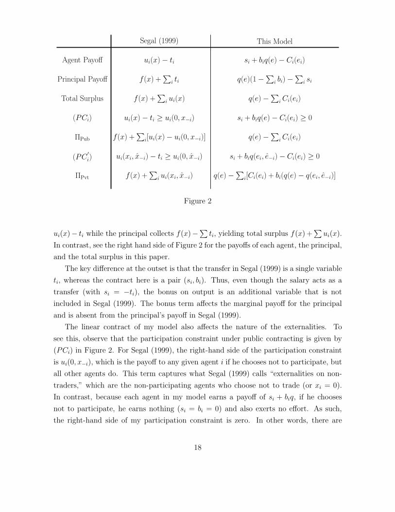
It is worthwhile to compare my results with those of Segal (1999), the chief paper that

has established the theoretical groundwork on contracting with externalities. Broadly

speaking, my model both is, and is not, an extension of Segal (1999). To see this, please

see Figure 2, which lists both models in a side-by-side comparison.

Segal (1999) examines a class of contracting models with quasi-linear utility. While

this class is broad, it does not perfectly capture the team incentive framework. A group

of n agents contracts over outcome x = (xi) with transfers ti to agent i. Each agent earns

17

Segal (1999) This Model

Agent Payoff ui(x)− ti si + biq(e)− Ci(ei)

Principal Payoff f(x) +∑

i ti q(e)(1−∑

i bi)−∑

i si

Total Surplus f(x) +∑

i ui(x) q(e)−∑

iCi(ei)

(PCi) ui(x)− ti ≥ ui(0, x−i) si + biq(e)− Ci(ei) ≥ 0

ΠPub f(x) +∑

i[ui(x)− ui(0, x−i)] q(e)−∑

iCi(ei)

(PC′i) ui(xi, x−i)− ti ≥ ui(0, x−i) si + biq(ei, e−i)− Ci(ei) ≥ 0

ΠPvt f(x) +∑

i ui(xi, x−i) q(e)−∑

i[Ci(ei) + bi(q(e)− q(ei, e−i)]

Figure 2

ui(x)− ti while the principal collects f(x)−∑

ti, yielding total surplus f(x) +∑

ui(x).

In contrast, see the right hand side of Figure 2 for the payoffs of each agent, the principal,

and the total surplus in this paper.

The key difference at the outset is that the transfer in Segal (1999) is a single variable

ti, whereas the contract here is a pair (si, bi). Thus, even though the salary acts as a

transfer (with si = −ti), the bonus on output is an additional variable that is not

included in Segal (1999). The bonus term affects the marginal payoff for the principal

and is absent from the principal’s payoff in Segal (1999).

The linear contract of my model also affects the nature of the externalities. To

see this, observe that the participation constraint under public contracting is given by

(PCi) in Figure 2. For Segal (1999), the right-hand side of the participation constraint

is ui(0, x−i), which is the payoff to any given agent i if he chooses not to participate, but

all other agents do. This term captures what Segal (1999) calls “externalities on non-

traders,” which are the non-participating agents who choose not to trade (or xi = 0).

In contrast, because each agent in my model earns a payoff of si + biq, if he chooses

not to participate, he earns nothing (si = bi = 0) and also exerts no effort. As such,

the right-hand side of my participation constraint is zero. In other words, there are

18

no externalities on non-traders here. This affects the principal’s profit function under

public contracts, expressed as ΠPub in Figure 2. For Segal (1999), the residual term

ui(0, x−i) constrains the principal’s profit function and will distort the optimal choice

away from efficiency. Since externalities on non-traders are absent here, the principal’s

payoff under public contracts is equal to total surplus. This is why I can obtain efficiency

under public contracting, as the linear contract eliminates externalities on non-traders,

and therefore public contracting maximizes total surplus.

Finally, the two models are more similar under private contracting. Observe the

participation constraint (PC ′i) under private contracting, shown in Figure 2. For Segal

(1999), the right-hand side is ui(0, x−i): the payoff to an agent who does not participate,

even though all other agents continue to trade at their equilibrium levels x−i. The

principal’s profit under private contracting in both Segal (1999) and here includes the

equilibrium term x−i for Segal (1999) and e−i for my model, and this in general will

distort choices away from efficiency. The principal’s payoff under private contracting

here includes the externality term q(e) − q(ei, e−i), whereas this is absent from the

corresponding payoff from Segal (1999).

Segal (1999) also gives general conditions comparing public and private contracting.

Let’s consider these in turn. First, he shows that if externalities are absent at an efficient

trade profile, private contracting produces efficient outcomes, regardless of externalities

that may exist at other trade profiles. This result is also true here and in fact has a

similar simple proof. If there exists an e∗ such that q(e∗i , e−i) does not depend on e−i

for all i, then observe that for any equilibrium of the private game, the equilibrium

condition reduces to

q(e)−∑

Ci(ei) ≥ q(e∗)−∑[

Ci(ei)+bi

{q(e∗)−q(e∗i , e−i)

}]= q(e∗)−

∑Ci(e

∗i ) (17)

and therefore this equilibrium is efficient. Of course, this assumption is quite strong,

in that the production function cannot depend on the actions of other agents, which is

unlikely to hold in realistic settings. So in this case, our model fits that of Segal (1999).

However, Segal (1999) further shows that if the agent’s utility function is additively

separable in xi and x−i, then public and private contracting coincide. The corresponding

assumption here is additive separability in the production function, which Proposition 3

and Corollary 2 has already shown makes private contracting differ from efficiency. And

because public contracting is identical to efficiency, this means that private and public

contracting in this model will differ.

19

Indeed, it is somewhat curious that the exact same assumption, additive separability,

generates precisely opposite conclusions in Segal (1999) and here. Yet on inspection, this

is not surprising. Because there are no externalities for non-traders (non-participating

agents), public contracting and efficiency are identical. So, the bilateral public offers

here generate efficient outcomes. The private contract generates budget balance, which

Proposition 1 shows introduces inefficiency. Thus, the linear wage schedule forces a

difference between public and private contracts. Segal (1999), on the other hand, does

involve externalities on non-participating agents, causing public contracts to deviate

from efficiency, and occasionally can actually coincide with private contracting.

An open question is how my results would change under more general, nonlinear

contracts. Overall, precise results are difficult to obtain without specifying the functional

form of the nonlinearity. I am able to obtain some fairly general results which are similar

in spirit to Segal (1999).9

4 Complementarity in Production

Now consider the analysis under complementarity, in which one agent’s effort can explic-

itly affect another agent’s equilibrium effort choice. In general, this problem becomes

complex, since complementarity introduces many interaction terms between agents. To

fix ideas, consider the general case of full complementarity.

Definition 4 The production function q has full complementarity if q(e) =∏n

i=1 βiei.

The parameter βi tracks the strength of the complementarity between agents. As

each βi grows, the effect of agent i on agent j increases. Throughout, let β =∏

i βi be

the product of these complementarity weights.

Observe that the marginal effect of any given agent’s effort on joint output is given

by qi(e) = βi

∏j 6=i βjej . Therefore all other agents j 6= i will affect any given agent’s

impact on joint output. This extreme case of complementarity binds all agents together.

Indeed, the incentive constraint in this case collapses to

C ′(ei) = biβi

∏

j 6=i

βjej . (18)

9Details of this nonlinear analysis are available from the author upon request and will be posted in

an online appendix.

20

In this specific setting with arbitrary number of agents, the number of possible in-

teraction effects precludes closed form solutions. However, the case with n = 3 is

remarkably elegant and generates a precise solution.

Proposition 4 If q has full complementarity, under three identical agents and quadratic

costs, the equilibrium is

b =β√

β + 2βand e =

√β + 2β

β√β

. (19)

Equilibrium effort is distorted above first-best (e > e∗). If β = 1, then budget balance

holds in the equilibrium of the bilateral private contracting game.

Three agents allow a closed form expression for equilibrium effort as a function of

the primitives of the model, namely, the complementarity parameters βi and the bonus

coefficient b. The expression for each agent’s effort is e =(β√∏

j 6=i bj

)−1

. It is easy to

see that each agent’s bonus has no effect on his effort level (∂ei∂bi

= 0), while the bonus of

other agent’s j 6= i has a negative effect on his effort level ( ∂ei∂bj

< 0). This is precisely the

consequence of complementarity: when the principal raises the bonus on other agents,

this induces agent i to shirk, since the higher bonus now allows the agent to gain benefit

without exerting costly effort.

As illustrated before, the principal’s objective function is the sum of total surplus and

the sum of the externalities of all other agents on each agent. Solving this optimization

under full complementarity and three agents leads to several simplifications. First,

Ei = 0 and ∂Ei

∂bi= 0 for any production function at equilibrium. More importantly,

the null effect of the bonus on any individual agent effort (∂ei∂bi

= 0) markedly simplifies

the first order conditions. Furthermore, under identical agents the first order condition

provides a unique solution for effort

(e = 1

b√β

)as a function of the bonus coefficient

b and β, the product of the βi. Combining this with the incentive constraint generates

a unique solution for bonus and effort as a function of β, given in the statement of

proposition. The proof shows that the bonus increases in β while the equilibrium effort

decreases in β. This should be intuitive: as the complementarity between different

agents increases, their productivity grows and their value to the firm increases, so the

principal increases the bonus in response. However, because of this complementarity,

the total effect on effort will fall since increasing any other individual’s bonus decreases

that individual’s effort ( ∂ei∂bj

< 0).

21

0 2 4 6 8

0.2

0.3

0.4

β

Equilibrium

Bon

us

0 2 4 6 80

5

10

15

β

Equilibrium

Effort

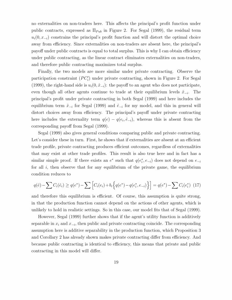
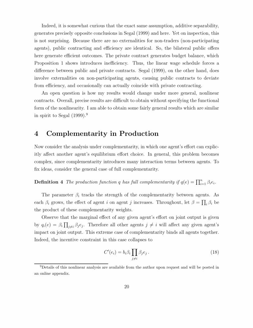
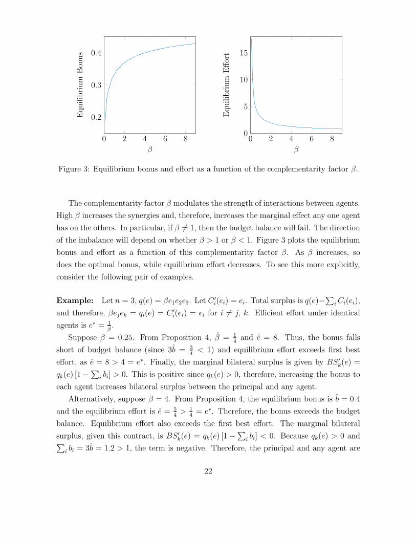
Figure 3: Equilibrium bonus and effort as a function of the complementarity factor β.

The complementarity factor β modulates the strength of interactions between agents.

High β increases the synergies and, therefore, increases the marginal effect any one agent

has on the others. In particular, if β 6= 1, then the budget balance will fail. The direction

of the imbalance will depend on whether β > 1 or β < 1. Figure 3 plots the equilibrium

bonus and effort as a function of this complementarity factor β. As β increases, so

does the optimal bonus, while equilibrium effort decreases. To see this more explicitly,

consider the following pair of examples.

Example: Let n = 3, q(e) = βe1e2e3. Let C′i(ei) = ei. Total surplus is q(e)−

∑i Ci(ei),

and therefore, βejek = qi(e) = C ′i(ei) = ei for i 6= j, k. Efficient effort under identical

agents is e∗ = 1β.

Suppose β = 0.25. From Proposition 4, β = 14and e = 8. Thus, the bonus falls

short of budget balance (since 3b = 34< 1) and equilibrium effort exceeds first best

effort, as e = 8 > 4 = e∗. Finally, the marginal bilateral surplus is given by BS ′k(e) =

qk(e) [1−∑

i bi] > 0. This is positive since qk(e) > 0, therefore, increasing the bonus to

each agent increases bilateral surplus between the principal and any agent.

Alternatively, suppose β = 4. From Proposition 4, the equilibrium bonus is b = 0.4

and the equilibrium effort is e = 54> 1

4= e∗. Therefore, the bonus exceeds the budget

balance. Equilibrium effort also exceeds the first best effort. The marginal bilateral

surplus, given this contract, is BS ′k(e) = qk(e) [1−

∑i bi] < 0. Because qk(e) > 0 and

∑i bi = 3b = 1.2 > 1, the term is negative. Therefore, the principal and any agent are

22

better off re-contracting to a lower bonus, since this will increase the bilateral surplus. �

Observe the following features of the prior example. First, if the complementarity

factor is low (with β = 14), then the optimal bonus falls short of budget balance. In

this case, the contract is not bilaterally efficient since the principal can increase bilateral

surplus by increasing the bonus. This would benefit the principal and any one agent,

and therefore, would make the pair better off. This is why the equilibrium of the

private contracting game is not bilaterally efficient, and illustrates the difference between

Proposition 4 and Corollary 1.

Similarly, with a high complementarity factor (of β = 4), the bonus exceeds budget

balance. It is still the case that equilibrium effort exceeds first best effort. This shows

that the effort distortion is a feature of the production function rather than the comple-

mentarity factor β. At this contract, the marginal bilateral surplus is negative, so the

principal and any one agent is jointly better off with a lower bonus.

5 Conclusion

The problem of free riding has plagued teams ever since the dawn of time. But it was

Holmstrom (1982) who first cast the fundamental tension between efficiency and budget

balance: the requirement that the sum of output-contingent pay granted to individual

team members equal total aggregate output, a common feature of partnerships. Nonethe-

less, Holmstrom proposed a solution of a “budget breaker,” in which a third party (the

principal) acts as a non-productive member of the team who coordinates contracting,

finances the bonuses, and acts as a sink on the output of all agents. By including a

budget breaker, the team achieves efficient production and still satisfies budget balance

over the team that now includes the principal. Yet this solution has both conceptual

and practical difficulties. The transfer payments from the agents violate endowment (or

limited liability) constraints. But more importantly, the budget breaker solution falls

apart if the principal can contract privately with the agents. This paper explores the

consequences to team production under two alternative contracting regimes, public and

private contracting.

The key insight of this analysis is that private contracting prevents collusion between

the principal and the agent. This collusion is exactly what breaks the public contracting

equilibrium. The only contracts that survive these rounds of private contracts are budget

23

balancing contracts, providing a justification for the budget balance constraint which the

team incentive literature has largely taken as given.

Future research in this area will explore more fully the consequences of private con-

tracting, which characterizes most employment settings. For example, any number of

contracting environments (such as corporate boards contracting with executives, man-

agers contracting with their superiors, or contracts between firms in the supply chain)

are all open to further analysis when the contracts are private. This just scratches the

surface of a new literature which could more closely resemble the information environ-

ments faced in practice.

6 Appendix

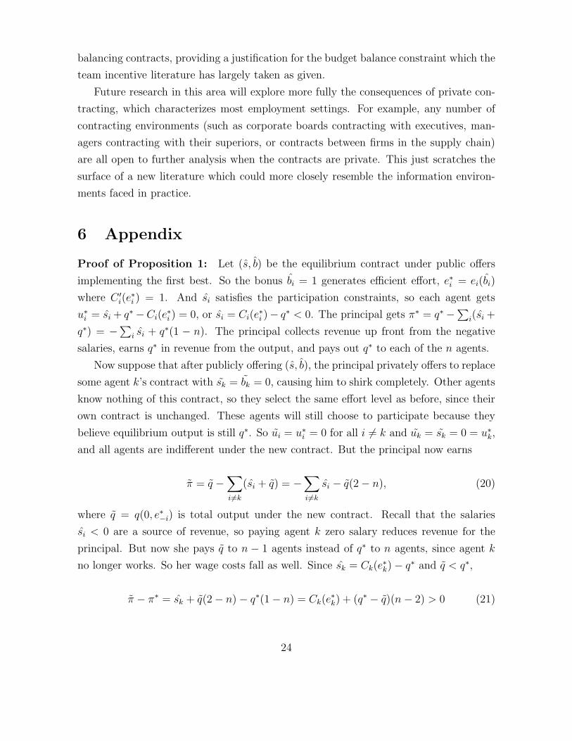
Proof of Proposition 1: Let (s, b) be the equilibrium contract under public offers

implementing the first best. So the bonus bi = 1 generates efficient effort, e∗i = ei(bi)

where C ′i(e

∗i ) = 1. And si satisfies the participation constraints, so each agent gets

u∗i = si + q∗ −Ci(e

∗i ) = 0, or si = Ci(e

∗i )− q∗ < 0. The principal gets π∗ = q∗ −∑i(si +

q∗) = −∑

i si + q∗(1 − n). The principal collects revenue up front from the negative

salaries, earns q∗ in revenue from the output, and pays out q∗ to each of the n agents.

Now suppose that after publicly offering (s, b), the principal privately offers to replace

some agent k’s contract with sk = bk = 0, causing him to shirk completely. Other agents

know nothing of this contract, so they select the same effort level as before, since their

own contract is unchanged. These agents will still choose to participate because they

believe equilibrium output is still q∗. So ui = u∗i = 0 for all i 6= k and uk = sk = 0 = u∗

k,

and all agents are indifferent under the new contract. But the principal now earns

π = q −∑

i 6=k

(si + q) = −∑

i 6=k

si − q(2− n), (20)

where q = q(0, e∗−i) is total output under the new contract. Recall that the salaries

si < 0 are a source of revenue, so paying agent k zero salary reduces revenue for the

principal. But now she pays q to n − 1 agents instead of q∗ to n agents, since agent k

no longer works. So her wage costs fall as well. Since sk = Ck(e∗k)− q∗ and q < q∗,

π − π∗ = sk + q(2− n)− q∗(1− n) = Ck(e∗k) + (q∗ − q)(n− 2) > 0 (21)

24

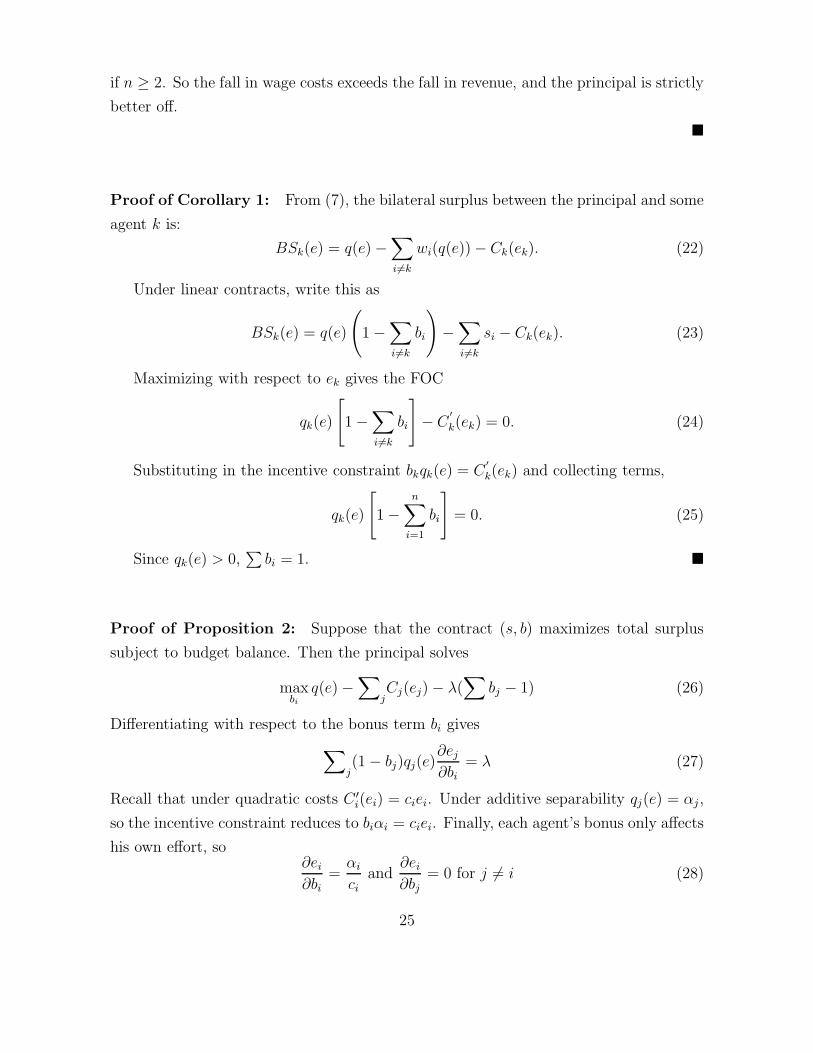
if n ≥ 2. So the fall in wage costs exceeds the fall in revenue, and the principal is strictly

better off.

�

Proof of Corollary 1: From (7), the bilateral surplus between the principal and some

agent k is:

BSk(e) = q(e)−∑

i 6=k

wi(q(e))− Ck(ek). (22)

Under linear contracts, write this as

BSk(e) = q(e)

(1−

∑

i 6=k

bi

)−∑

i 6=k

si − Ck(ek). (23)

Maximizing with respect to ek gives the FOC

qk(e)

[1−

∑

i 6=k

bi

]− C

′

k(ek) = 0. (24)

Substituting in the incentive constraint bkqk(e) = C′

k(ek) and collecting terms,

qk(e)

[1−

n∑

i=1

bi

]= 0. (25)

Since qk(e) > 0,∑

bi = 1. �

Proof of Proposition 2: Suppose that the contract (s, b) maximizes total surplus

subject to budget balance. Then the principal solves

maxbi

q(e)−∑

jCj(ej)− λ(

∑bj − 1) (26)

Differentiating with respect to the bonus term bi gives

∑j(1− bj)qj(e)

∂ej

∂bi= λ (27)

Recall that under quadratic costs C ′i(ei) = ciei. Under additive separability qj(e) = αj ,

so the incentive constraint reduces to biαi = ciei. Finally, each agent’s bonus only affects

his own effort, so∂ei

∂bi=

αi

ciand

∂ei

∂bj= 0 for j 6= i (28)

25

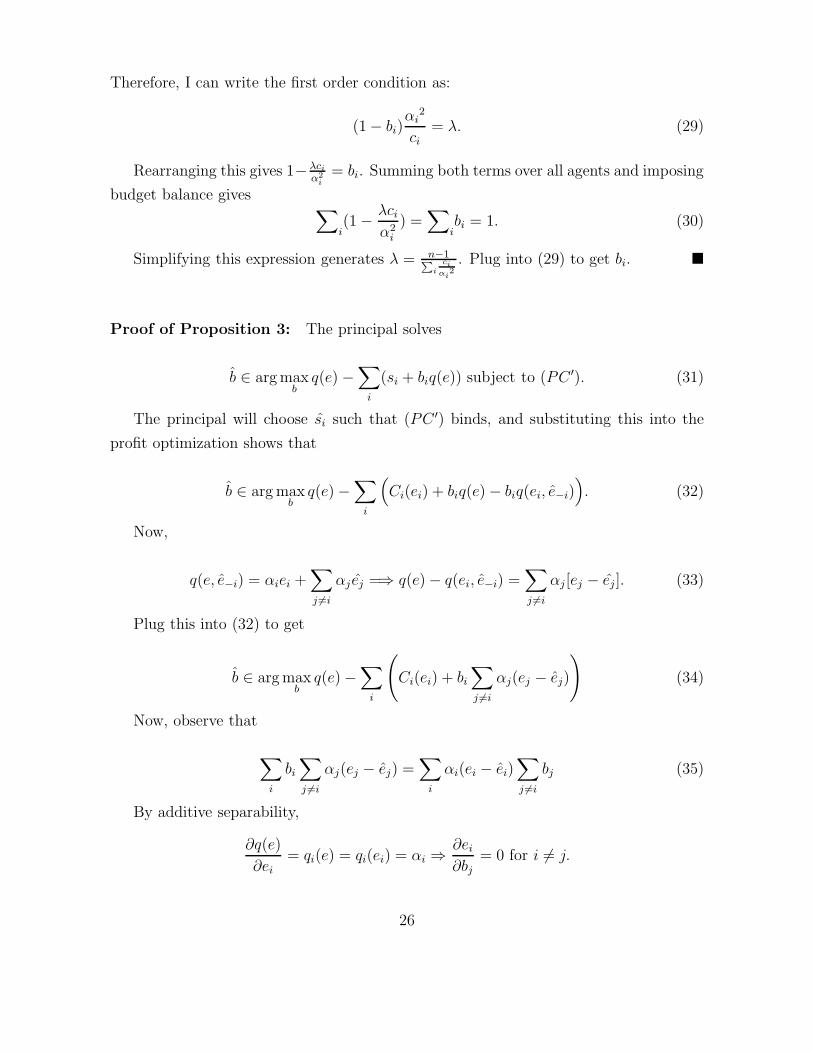
Therefore, I can write the first order condition as:

(1− bi)αi

2

ci= λ. (29)

Rearranging this gives 1− λciα2

i

= bi. Summing both terms over all agents and imposing

budget balance gives ∑i(1− λci

α2i

) =∑

ibi = 1. (30)

Simplifying this expression generates λ = n−1∑i

ciαi

2

. Plug into (29) to get bi. �

Proof of Proposition 3: The principal solves

b ∈ argmaxb

q(e)−∑

i

(si + biq(e)) subject to (PC ′). (31)

The principal will choose si such that (PC ′) binds, and substituting this into the

profit optimization shows that

b ∈ argmaxb

q(e)−∑

i

(Ci(ei) + biq(e)− biq(ei, e−i)

). (32)

Now,

q(e, e−i) = αiei +∑

j 6=i

αj ej =⇒ q(e)− q(ei, e−i) =∑

j 6=i

αj [ej − ej ]. (33)

Plug this into (32) to get

b ∈ argmaxb

q(e)−∑

i

(Ci(ei) + bi

∑

j 6=i

αj(ej − ej)

)(34)

Now, observe that

∑

i

bi∑

j 6=i

αj(ej − ej) =∑

i

αi(ei − ei)∑

j 6=i

bj (35)

By additive separability,

∂q(e)

∂ei= qi(e) = qi(ei) = αi ⇒

∂ei

∂bj= 0 for i 6= j.

26

So the derivative of this objective function (34) with respect to bk is

∂π

∂ek

∂ek

∂bk+

∂π

∂bk=

[αk − C ′

k(ek)− αk

∑

i 6=k

bi

]∂ek

∂bk−∑

j 6=k

αj(ej − ej). (36)

The FOC requires this derivative evaluated at the equilibrium b, to equal zero. So

ej = ej(bj) and the last sum on the right vanishes, so

[αk − C ′

k(ek)−∑

i 6=k

bi

]∂ek∂bk

= 0. (37)

Combining with (IC) gives∑

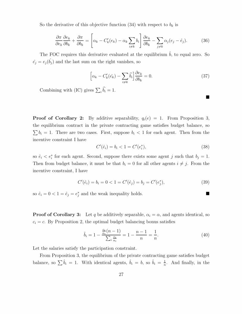
i bi = 1.

�

Proof of Corollary 2: By additive separability, qi(e) = 1. From Proposition 3,

the equilibrium contract in the private contracting game satisfies budget balance, so∑

bi = 1. There are two cases. First, suppose bi < 1 for each agent. Then from the

incentive constraint I have

C ′(ei) = bi < 1 = C ′(e∗i ), (38)

so ei < e∗i for each agent. Second, suppose there exists some agent j such that bj = 1.

Then from budget balance, it must be that bi = 0 for all other agents i 6= j. From the

incentive constraint, I have

C ′(ei) = bi = 0 < 1 = C ′(ej) = bj = C ′(e∗j ), (39)

so ei = 0 < 1 = ej = e∗j and the weak inequality holds. �

Proof of Corollary 3: Let q be additively separable, αi = α, and agents identical, so

ci = c. By Proposition 2, the optimal budget balancing bonus satisfies

bi = 1−ciαi(n− 1)∑

iciαi

= 1− n− 1

n=

1

n. (40)

Let the salaries satisfy the participation constraint.

From Proposition 3, the equilibrium of the private contracting game satisfies budget

balance, so∑

bi = 1. With identical agents, bi = b, so bi = 1n. And finally, in the

27

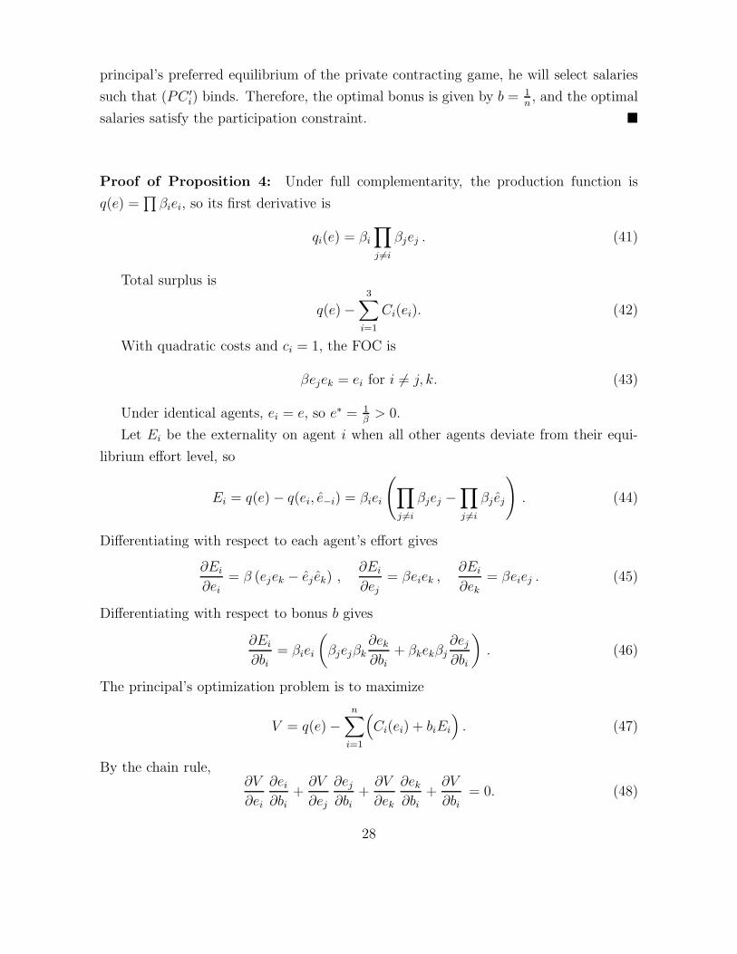
principal’s preferred equilibrium of the private contracting game, he will select salaries

such that (PC ′i) binds. Therefore, the optimal bonus is given by b = 1

n, and the optimal

salaries satisfy the participation constraint. �

Proof of Proposition 4: Under full complementarity, the production function is

q(e) =∏

βiei, so its first derivative is

qi(e) = βi

∏

j 6=i

βjej . (41)

Total surplus is

q(e)−3∑

i=1

Ci(ei). (42)

With quadratic costs and ci = 1, the FOC is

βejek = ei for i 6= j, k. (43)

Under identical agents, ei = e, so e∗ = 1β> 0.

Let Ei be the externality on agent i when all other agents deviate from their equi-

librium effort level, so

Ei = q(e)− q(ei, e−i) = βiei

(∏

j 6=i

βjej −∏

j 6=i

βj ej

). (44)

Differentiating with respect to each agent’s effort gives

∂Ei

∂ei= β (ejek − ej ek) ,

∂Ei

∂ej= βeiek ,

∂Ei

∂ek= βeiej . (45)

Differentiating with respect to bonus b gives

∂Ei

∂bi= βiei

(βjejβk

∂ek

∂bi+ βkekβj

∂ej

∂bi

). (46)

The principal’s optimization problem is to maximize

V = q(e)−n∑

i=1

(Ci(ei) + biEi

). (47)

By the chain rule,∂V

∂ei

∂ei

∂bi+

∂V

∂ej

∂ej

∂bi+

∂V

∂ek

∂ek

∂bi+

∂V

∂bi= 0. (48)

28

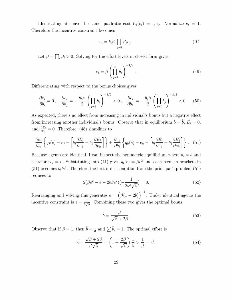
Identical agents have the same quadratic cost Ci(ei) = ciei. Normalize ci = 1.

Therefore the incentive constraint becomes

ei = biβi

∏

j 6=i

βjej . (IC)

Let β =∏

i βi > 0. Solving for the effort levels in closed form gives

ei = β

(n∏

j 6=i

bj

)−1/2

. (49)

Differentiating with respect to the bonus choices gives

∂ei

∂bi= 0 ,

∂ei

∂bj= − bkβ

2

(∏

j 6=i

bj

)−3/2

< 0 ,∂ei

∂bk= − bjβ

2

(∏

j 6=i

bj

)−3/2

< 0 (50)

As expected, there’s no effect from increasing in individual’s bonus but a negative effect

from increasing another individual’s bonus. Observe that in equilibrium b = b, Ei = 0,

and ∂Ei

∂ei= 0. Therefore, (48) simplifies to

∂ej

∂bi

{qj(e)− ej −

[bi∂Ei

∂ej+ bk

∂Ek

∂ek

]}+

∂ek

∂bi

{qk(e)− ek −

[bi∂Ei

∂ek+ bj

∂Ej

∂ek

]}. (51)

Because agents are identical, I can inspect the symmetric equilibrium where bi = b and

therefore ei = e. Substituting into (41) gives qi(e) = βe2 and each term in brackets in

(51) becomes bβe2. Therefore the first order condition from the principal’s problem (51)

reduces to

2(βe2 − e− 2bβe2)(− 1

2b2√β) = 0. (52)

Rearranging and solving this generates e =(β(1 − 2b)

)−1

. Under identical agents the

incentive constraint is e = 1b√β. Combining these two gives the optimal bonus

b =β√

β + 2β. (53)

Observe that if β = 1, then b = 13and

∑bi = 1. The optimal effort is

e =

√β + 2β

β√β

=

(1 +

2β√β

)1

β>

1

β= e∗. (54)

29

Now

∂b

∂β=

√β − β

2√β(√

β + 2β)2 > 0. (55)

And ∂e∂β

< 0 since 2β + 2β√β > 0.

�

30

7 References

1. Baldenius, T.; S. Dutta; and S. Reichelstein. “Cost Allocation for Capital Budgeting

Decisions.” The Accounting Review (2007): 837-867.

2. Demski, J. S. 1981. Cost allocation games. Joint Cost Allocations, edited by S. Mori-

arity, 142-73. Center for Economic and Management Research, University of Oklahoma,

Norman.

3. Eswaran, Mukesh, and Ashok Y. Kotwal. 1984. “The Moral Hazard of Budget-

Breaking.” Rand Journal of Economics, 15(4): 578-81.

4. Holmstrom, B. “Moral Hazard in Teams.” Bell Journal of Economics 13 (1982):

324-340.

5. Holmstrom, B., and P. Milgrom. “Regulating Trade Among Agents.” Journal of

Institutional and Theoretical Economics (1990): 85-105.

6. Huddart, S., and P. J. Liang. “Profit sharing and monitoring in partnerships.”

Journal of Accounting and Economics 40 (2005): 153-187.

7. Itoh, H. “Coalitions, incentives, and risk sharing.” Journal of Economic Theory 60

(1993): 410-427.

8. Kofman, F., and J. Lawarree. “Collusion in hierarchical agency.” Econometrica:

Journal of the Econometric Society (1993): 629-656.

9. Lazear EP, and Rosen S. “Rank-Order Tournaments as Optimum Labor Contracts.”

Journal of Political Economy 89(1981): 841-864.

10. Legros, P., and H. Matsushima. “Efficiency in partnerships.” Journal of Economic

Theory 55 (1991): 296-322.

11. Legros, P., and S. Matthews. “Efficient and nearly-efficient partnerships.” The

Review of Economic Studies 60 (1993): 599-611.

12. Macho-Stadler, I., and J. D. Perez-Castrillo. “Moral hazard with several agents: The

gains from cooperation.” International Journal of Industrial Organization 11 (1993): 73-

100.

13. McAfee, R. P., and M. Schwartz. “Opportunism in Multilateral Vertical Contracting:

Nondiscrimination, Exclusivity, and Uniformity.” The American Economic Review 84

(1994): 210230.

14. Miller, N. “Efficiency in partnerships with joint monitoring.” Journal of Economic

Theory 77 (1997): 285-299.

15. Rajan, M. “Cost allocation in multiagent settings.” The Accounting Review (1992):

31

527-545.

16. Ramakrishnan, R. T., and A. V. Thakor. “Cooperation versus competition in

agency.” Journal of Law, Economics, and Organization (1991): 248-283.

17. Rasmusen, E. “Moral hazard in risk-averse teams.” The RAND Journal of Economics

(1987): 428-435.

18. Ray, K., and M. Goldmanis. “Efficient Cost Allocation.” Management Science

(2012): 1341-1356.

19. Segal, I. “Contracting with Externalities.” The Quarterly Journal of Economics 114

(1999): 337388.

20. Segal, I., and M. D. Whinston. “Robust Predictions for Bilateral Contracting with

Externalities.” Econometrica 71 (2003): 757791.

21. Varian, H. “Monitoring agents with other agents.” Journal of Institutional and

Theoretical Economics (1990): 153-174.

32