technical analysis, momentum and autocorrelationchesler.us/resources/academia/technical analysis,...
TRANSCRIPT
1
Technical Analysis, Momentum and Autocorrelation
K. J. Honga and S.Satchell
b
Working Paper Aug 24, 2011
a Queens’ College, University of Cambridge
Tel: 44 777 594 3238 E-mail: [email protected]
Address: Queens’ College, Cambridge CB3 9ET, UK
b Trinity College, University of Cambridge
Tel: 44 12233 38409 E-mail: [email protected]
Address: Trinity College, Cambridge, CB2 1TQ, U.K.
Abstract
This article assumes general stationary processes for prices and derives the autocorrelation
function for a general Moving Average (MA) trading rule to investigate why this rule is used.
The result shows that the MA rule is popular because it can identify the price momentum and
is a simple way of tracing and exploiting the price autocorrelation structure without actually
knowing it. We focus on analyzing the impact of price momentum on the profitability of the
MA rule because the price momentum effect tends to be stronger and longer-lived than the
return momentum effect.

2
1 Introduction
While fundamental analysts study a company’s underlying indicators of profit such as
earnings, dividends, new products and R&D, technical analysts focus mainly on price and
return but, unwittingly or otherwise, also examine psychological aspects in the demand for a
company’s stock. Technicians employ many techniques, one of which is the use of charts.
Using charts, technical analysts seek to identify price patterns and market trends in financial
markets and attempt to exploit these patterns. Traders and portfolio managers continue to use
technical analysis that forecast stock price movements using historical prices to formulate
buy and sell decisions. Empirical studies report supporting evidence for the profitability of
technical analysis, including Sweeney (1986, 1988), Brock et al. (1992), Blume et al. (1994),
Chan, Jegadeesh, and Lakonishok (1996), Gencay (1996, 1998, 1999), Neely et al. (1997),
Brown et al. (1998), Rouwenhorst (1998), Allen and Karjalainen (1999), Chang and Osler
(1999), Neely and Weller (1999), Chan et al. (2000), Shleifer (2000), and Lo et al. (2000).
These results suggest that technical analysis beat the market in risk neutral terms, hence its
popularity.
One of the simplest and most widely used trading strategies based on technical analysis is
the Moving Average (MA) rule, which is an objective rule-based trading strategy in which
buy and sell signals are determined by the relative magnitudes of short and long term MAs.
An objective rule-based trading system has well-defined and indisputable buy and sell signals
following a decision rule based on past data. The MA rule often leads investors to invest with
or against the trend, or momentum since it assumes that prices trend directionally. The
profitability of the MA rule has been heavily investigated in the previous literature. Brook,
Lakonishock and LeBaron (1992) suggested evidence that technical trading rules have
predictive ability with respect to market indices in the USA in both conditional means and
variances. Further, they showed that these results were relatively stable over their 90 year
sample period. Hudson et al. (1996) did the same for market indices in the UK. Gunasekarage
and Power (2000) indicated that the employment of these techniques also generates excess
returns to investors in South Asian markets. Reitz (2006) shows that self-fulfilling
expectations and herd behavior not only re-confirm the profitability of technical trading rules,
but also put forward a sensible explanation as to why such rules may actually work.
The MA rule takes advantage of price trend, which is closely linked with the rather
nebulous idea of price momentum. The profitability of price momentum strategies, initially

3
investigated by Jegadeesh and Titman (1993), has received the most attention among all the
anomalies examined by Fama and French (1996). It is the fourth anomaly included in the
Carhart four-factor model. Jegadeesh and Titman (2001) argue that their 1993 results are not
due to data mining since the monthly momentum strategy profit is about 1% in the 1990s.
Furthermore, Rouwenhorst (1998) confirms the robustness of this strategy by showing that
between 1980 and 1995 an internationally diversified portfolio of past medium-term Winners
outperformed a portfolio of medium-term Losers after correcting for risk by more than one
percent per month. Specifically, Rouwenhorst (1998) finds significantly positive momentum
payoffs in 12 countries that he investigated. (Price) Momentum is defined by the above
authors as the product of the relative prices over the holding period and a past winners
strategy is to buy the top n-th of stocks with this characteristic in a portfolio. A careful
reading of the momentum literatures fails to find clarification over whether momentum is
present when the price of the asset follows (a) a random walk (b) a random walk with drift or
(c) a mean reverting process around a linear trend. The issue is further complicated by
different treatments for prices, returns and earnings. One of the purposes of this paper is to try
and understand the time series basis of a momentum strategy. We assume general stationary
processes for prices and derive the autocorrelation function for a general MA rule. We focus
on analyzing the impact of price momentum, instead of returns or earnings momentum, on
the profitability of the MA rule because (1) most of, if not all, trading rules using technical
analysis are based on past prices, and (2) the price momentum effect tends to be stronger and
longer-lived than the return momentum effect. Most previous momentum studies typically
include a large cross-section of stocks weighted by the previous period return. There exists
another type of price trend besides the momentum discussed, however. Equity prices tend to
show a long run market-wide trend. This can be dues to inflation or other economic
conditions. We define this market-wide trend by the parameter, µ. We remove the market-
wide trend from our price process in order to focus on price momentum only.
This paper presents a simple and straightforward evaluation of the MA rule with one
investor and one asset. To evaluate the MA rule, an exact definition of momentum is
required, which is presented in Section 2.2 with a statistical model. We find that that there are
two reasons why the MA rule is popular. First, the MA rule can identify the price momentum
(trend), which comfortably confirms the results of previous momentum literature. Second, the
MA rule is a simple way of tracing and exploiting the price autocorrelation structure without
actually knowing it. It is very hard, if not impossible, to know the real structure of the price

4
autocorrelation of an asset, and the MA rule provides a simple and clear methodology that
can take advantage of the price autocorrelation structure. The main contribution of this paper
is that we suggest two reasons why the technical trading strategy, or Chartism, is popular and
this leads to price autocorrelation. If a conservatism bias exists in a market, we can confirm
that the MA rule is profitable. A conservatism bias indicates that investors are too slow (too
conservative) in updating their beliefs in response to recent evidence. This means that they
might initially underreact to news about a firm, meaning that prices will fully reflect new
information only gradually. Such a bias would give rise to momentum (price autocorrelation)
in the stock market. Using AR (1) and MA (1) processes, we take the discussion away from
short term price trend continuation or long term price reversal. In short, it is not just about
buying past losers or winners but is also about identifying price trends and the autocorrelation
structure. This paper does not intend to explain all the reasons for the predictability nor does
it attempt to explain why arbitrage fails to eliminate mispricing. The rest of the paper is
organized as follows. Section 2 explains the trading rule and how it is related to price
momentum. Section 3 presents the general model. Section 4 shows the autocorrelation
structure of the trading strategy. Section 5 presents empirical evidence and Section 6
concludes the paper.
2 Trading Rule and Momentum
2.1 Trading Rules Definition
We employ and expand the definition of the MA oscillator by Brock et al. (1992), which
states: “According to the moving average trading rule, buy and sell signals are generated by
two moving averages of the level of the index – a long-period average and a short-period
average. In its simplest form this strategy is expressed as buying (or selling) when the short-
period moving average rises above (or falls below) the long-period moving average. The idea
behind computing moving averages it to smooth out an otherwise volatile series. When the
short-period average exceeds the long-period moving average, a trend is considered to be
initiated. A very popular moving average rule is 1-200, where the short period is one day and
the long period is 200 days. While numerous variations of this rule are used in practice, we
attempted to select several of the most popular ones: 1-50, 1-150, 5-150, 1-200, and 2-200.”
However, we can also take into consideration the flip side of the strategy, where we buy
5
when short-period MA falls below the long-period MA and we sell when the opposite
happens.
Let l stands for the time period that the MA is computed for a long position and s for the
time period that the MA is computed for a short position. Hence s > l and they overlap.
Denote SMA as MA computed over time period s and LMA as MA computed over time
period l. For example at time t, if s = 7 and l = 3, then SMA is computed over time t – 6 to t
and LMA is computed over time t – 2 to t. We classify two opposite MA rules with SMA and
LMA, MAbull(l,s) and MAbear(l,s), and define the MAbull(l,s) rule as taking a long position
in the asset when SMA > LMA and as taking no position in the asset when the SMA < LMA
and MAbear(l,s) rule does the opposite.
Definition 1: The MAbull(l,s) and MAbear(l,s) position can be represented as
( )0),(max),( tslMAbull δ= ( )0),(1max),( tslMAbear δ−=
where
<−
>−=
1)()( if 0
1)()( if 1)(
tSMAtLMA
tSMAtLMAtδ
and
s
itP
tSMA
s
i
∑=
+−= 1
)1(
)( and l
itP
tLMA
l
i
∑=
+−= 1
)1(
)(
The logic behind the MAbull rule is well known, when a price penetrates the MA from
below, the bull trend is believed to be established and a trader wants to take advantage of this
in the expectation that there will be further upward movements in prices. The MAbear rule
tells us the opposite story, short term price reversal. When the price falls enough to penetrate
the MA from the above, this might be due to the market over-reaction; hence a trader would
take a long position, expecting that the price would bounce immediately back.
2.2 Momentum Definition and a Statistical Model
It is very hard to find a formal definition of momentum that has a statistical basis. By this we
mean a definition of momentum defined as a property or properties of a stochastic process.
Much previous literature such as Brook et al. (1992), Barberis et al. (1998), Rowenhorst
(1998), Daniel et al. (1998), Hong and Stein (1999) Jegadeesh and Titman (2001) and Fong
6
and Yong (2005) explain momentum as an upward trend in a time series, which can be
assets’ prices, earnings or returns. But they concentrate only on historical data and do not
give explanations in terms of underlying processes. Technical analysts interpret momentum
in terms of moving averages; when the current price rises above its moving average it is
interpreted as an upward (bullish) trend , while a downward (bearish) trend emerges when the
current price falls below its moving average. These interpretations do not really clarify if
momentum is related to trend or to autocorrelation; both ideas having precise definitions in a
statistical sense.
We turn to the practitioner literature to see if matters are resolved. The definition of
momentum in Wikipedia is “Momentum investing, also sometimes known as "Fair Weather
Investing", is a system of buying stocks or other securities that have had high returns over the
past three to twelve months, and selling those that have had poor returns over the same
period.” And in Investopedia, momentum is defined as “An investment strategy that aims to
capitalize on the continuance of existing trends in the market. The momentum investor
believes that large increases in the price of a security will be followed by additional gains and
vice versa for declining values.” Achelis (2000) defines “The Momentum Indicator is the
ratio of today’s price compared to the price n periods ago: Momentum = (Close / Close n
periods ago) * 100. Therefore Momentum Investing is investing in securities with levels of
Momentum Indicator above certain threshold.” As quoted in Schwager (1992), Richard
Driehaus (who is widely regarded as the father of momentum investing) once said “far more
money is made buying high and selling at even higher prices” (as opposed to “buy low sell
high”).
The only definition of the above that has a clear mathematical structure is that of Achelis.
We shall take his definition and see if it can be consistent with standard dynamic stochastic
processes and, as a consequence, what the determinants of momentum will be. The obvious
candidate is the log Ornstein – Uhlenbeck (log OU) process. Although our work focuses on
price momentum, the same approach can be applied to other time series such as returns and
earnings.
Whilst momentum is attributed to behavioural explanations, typically herding and the
conservatism bias, we shall not look at equilibrium models with momentum investors in. On
the basis of previous definitions, momentum manifests itself in statistical models as possibly
either trend or autocorrelation or both. Therefore, we advocate the log Ornstein – Uhlenbeck
model to demonstrate this. This model can be thought of as a stationary process concerning a
7
trend or a random walk with drift or an explosive process about a trend. Such versatility
should allow us to gain some insights into the properties of momentum, as defined by
Achelis. Assume that the logarithm of the asset price ( ))(log tP has linear trends, tµ . We
consider the process
ttPtq µ−= )(log:)(
Assume a log price process,
)1()()()( tdWdttqtdq σθ +−=
The solution for equation (1) is well known,
( )( ) ( ) )2()((exp)(ln1exp)(ln)(ln ∫+
−−+−−+=−+ht
tudWttPhhtPhtP µθσθµ
h is the holding period, which is always positive. In this model, ( )θh−exp can be interpreted
as the degree of price autocorrelation. In fact, the model admits a autoregressive (AR(1))
representation in which this is the autoregressive coefficient. From well-known properties of
the AR(1) model , we know that stationarity and the existence of a steady-state solution
require 0>θ .Indeed, we can think of two different processes for equation (2) depending on
the magnitude of the autoregressive coefficient.. First, when equation (2) is mean reverting,
then ( ) 1exp <− θh (i.e. positive autocorrelation) and hence 0>θ . Second, when equation (2)
is explosive, then ( ) 1exp >− θh , there is neither stationarity nor a steady-state solution and
hence 0<θ
According to the definition of momentum proposed by Achelis, momentum can be
interpreted as the sensitivity of the expected price ratio with respect to today’s price. If this
sensitivity is positive then there is a bullish momentum and if negative there is a bearish
momentum.
Proposition 1: The derivative of conditional population momentum with respect to previous
period’s price can be expressed as
8
)3(1)exp()(ln
)(
)(ln
−−=∂
+∂
θhtP
tP
htPE
The proof of Proposition 1 is in Appendix A1. This clearly shows that, for log OU,
momentum is about autocorrelation. Equation (3) shows that when the price process is mean
reverting, the elasticity of momentum is negative while it is positive if the price is explosive.
This is exactly what we would anticipate. In other words, given the high past price, the future
price is low if the price process reverts around a mean but the future price is high if the price
process is explosive. If we were to interpret efficient markets as a log random walk with drift,
then the elasticity would become zero. Finally, the elasticity is independent of the trend.
2.3 The MA Rule and Price Momentum
The relationship between the MA rule and price momentum is well explained in Fong and
Yong (2005). “In the simplest form, a MA crossover rule operates on the assumption that buy
signals are generated when the current stock price crosses its moving average from below
while sell signals are generated when the stock price crosses its moving average from above.
The rationale for this interpretation is that a trend is said to have emerged when the stock
price penetrates the moving average. Specifically, an upward (bullish) trend emerges when
the price rises above its moving average, while a downward (bearish) trend emerges when the
price falls below its moving average.” Therefore, the MAbull rule takes advantage of the
bullish trend while the MAbear rule takes advantage of the bearish trend.
3 The Model
3.1 General Model
Let the de-meaned log price process ttPtq µ−= )(log)( has distribution ( )2,0~)( σtq . Also
denote the autocorrelation between )(tq and )( htq − as )(hAρ . Since we are using log prices,
it would be sensible to use geometric price MAs which are equivalent to arithmetic log price
MAs.
9
+−
=∑=
s
itq
tSMA
s
i 1
)1(
exp)( and
+−
=∑=
l
itq
tLMA
l
i 1
)1(
exp)( where ls >
Under such a framework, the return at time t is defined as
µ−−−=−− )1(log)(log)1()( tPtPtqtq
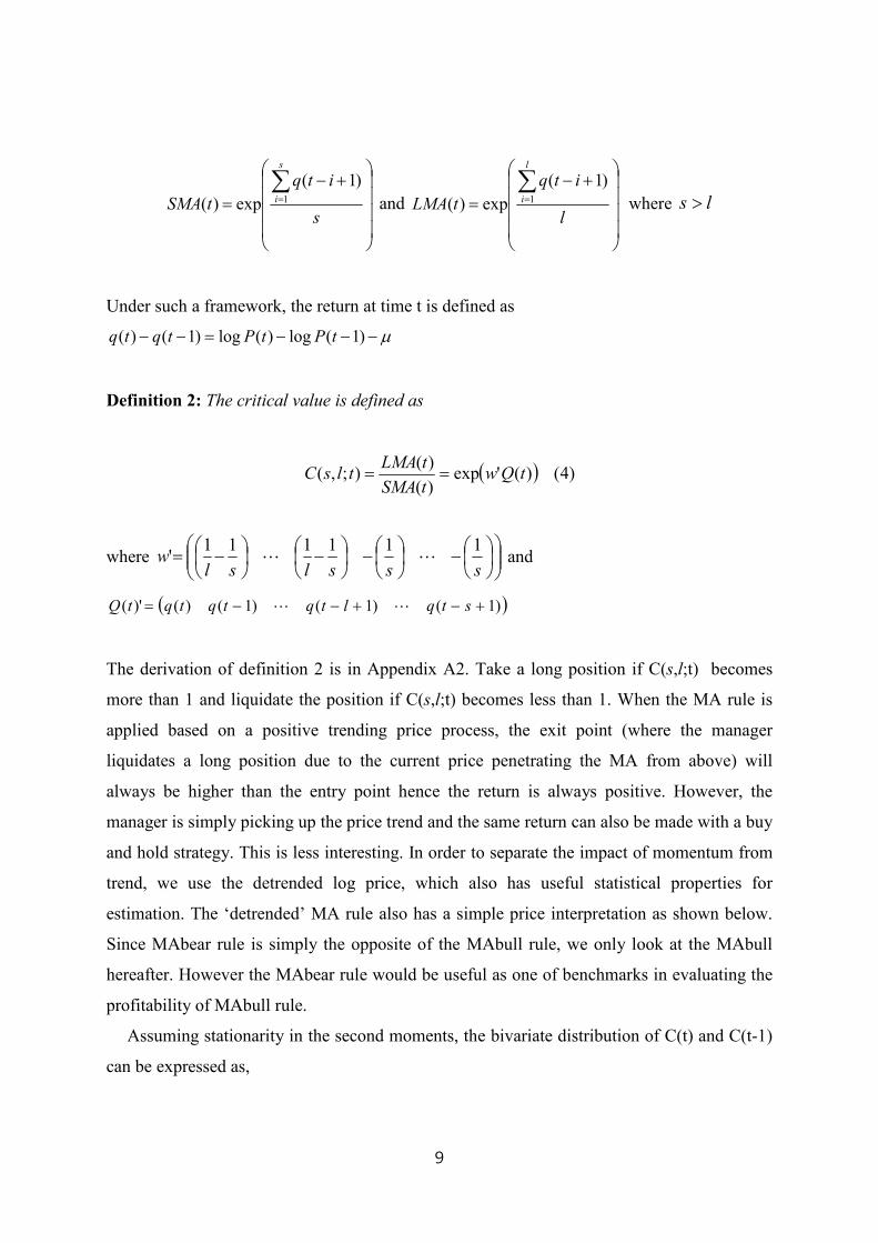
Definition 2: The critical value is defined as
where
−
−
−
−=ssslsl
w111111
' LL and
( ))1()1()1()()'( +−+−−= stqltqtqtqtQ LL
The derivation of definition 2 is in Appendix A2. Take a long position if C(s,l;t) becomes
more than 1 and liquidate the position if C(s,l;t) becomes less than 1. When the MA rule is
applied based on a positive trending price process, the exit point (where the manager
liquidates a long position due to the current price penetrating the MA from above) will
always be higher than the entry point hence the return is always positive. However, the
manager is simply picking up the price trend and the same return can also be made with a buy
and hold strategy. This is less interesting. In order to separate the impact of momentum from
trend, we use the detrended log price, which also has useful statistical properties for
estimation. The ‘detrended’ MA rule also has a simple price interpretation as shown below.
Since MAbear rule is simply the opposite of the MAbull rule, we only look at the MAbull
hereafter. However the MAbear rule would be useful as one of benchmarks in evaluating the
profitability of MAbull rule.
Assuming stationarity in the second moments, the bivariate distribution of C(t) and C(t-1)
can be expressed as,
( ) )4()('exp)(
)();,( tQw
tSMA
tLMAtlsC ==
10
ΩΩ
ΩΩ
− wwww
wwww-
mtQw
tQw
m
m
''
''
0
0~
)('
)('
where Ω is the (s × s) covariance matrix of Q(t) and CΩ is (s × s) covariance matrix
between Q(t) and Q(t-1). For now, we do not assume anything about the covariance matrix
but simply note that the autocovariance is not zero.
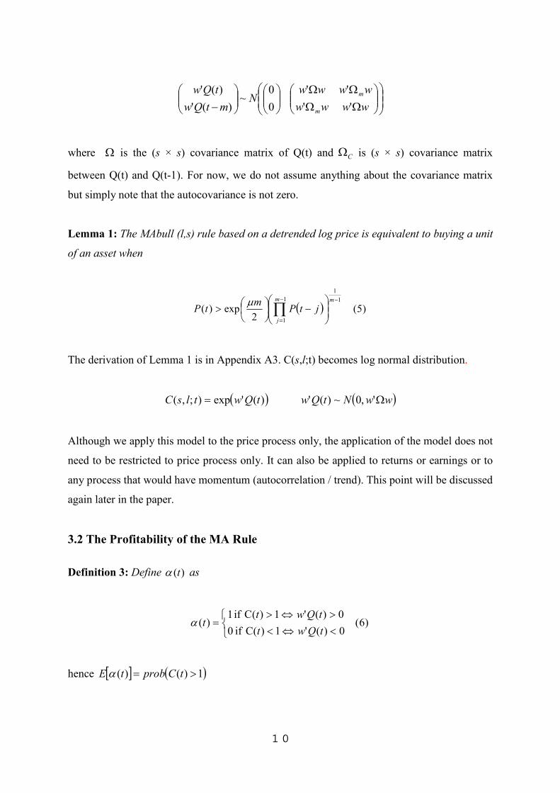
Lemma 1: The MAbull (l,s) rule based on a detrended log price is equivalent to buying a unit
of an asset when
( ) )5(2
exp)(1
1
1
1
−−
=
−
> ∏mm
j
jtPm
tPµ
The derivation of Lemma 1 is in Appendix A3. C(s,l;t) becomes log normal distribution.
( ))('exp);,( tQwtlsC = ( )ww-tQw Ω',0~)('
Although we apply this model to the price process only, the application of the model does not
need to be restricted to price process only. It can also be applied to returns or earnings or to
any process that would have momentum (autocorrelation / trend). This point will be discussed
again later in the paper.
3.2 The Profitability of the MA Rule
Definition 3: Define )(tα as
)6(0)('1)(C if 0
0)('1)(C if 1)(
<⇔<
>⇔>=
tQwt
tQwttα
hence [ ] ( )1)()( >= tCprobtE α
11
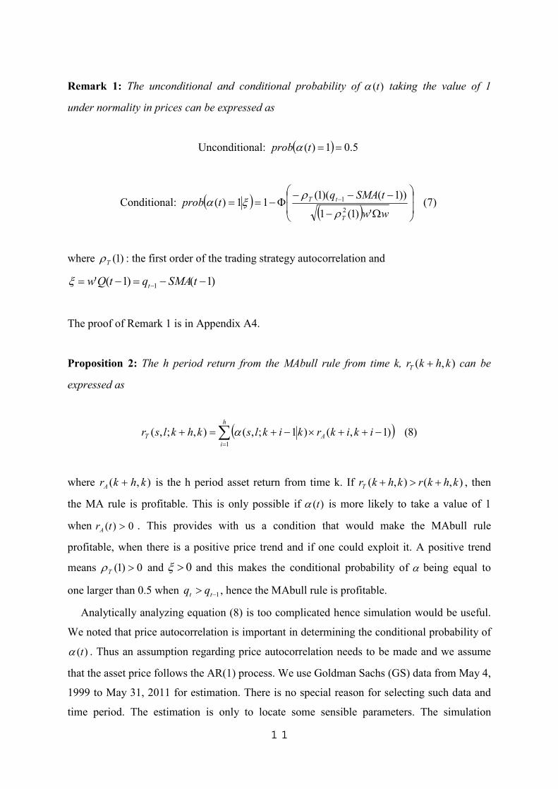
Remark 1: The unconditional and conditional probability of )(tα taking the value of 1
under normality in prices can be expressed as
Unconditional: ( ) 5.01)( ==tprob α
Conditional: ( )( )
)7(')1(1
))1()(1(11)(
2
1
Ω−
−−−Φ−== −
ww
tSMAqtprob
T
tT
ρ
ρξα
where )1(Tρ : the first order of the trading strategy autocorrelation and
)1()1(' 1 −−=−= − tSMAqtQw tξ
The proof of Remark 1 is in Appendix A4.
Proposition 2: The h period return from the MAbull rule from time k, ),( khkrT + can be
expressed as
( ) )8()1,()1;,(),;,(1
∑=
−++×−+=+h
i
AT ikikrkiklskhklsr α
where ),( khkrA + is the h period asset return from time k. If ),(),( khkrkhkrT +>+ , then
the MA rule is profitable. This is only possible if )(tα is more likely to take a value of 1
when 0)( >trA . This provides with us a condition that would make the MAbull rule
profitable, when there is a positive price trend and if one could exploit it. A positive trend
means 0)1( >Tρ and 0>ξ and this makes the conditional probability of α being equal to
one larger than 0.5 when 1−> tt qq , hence the MAbull rule is profitable.
Analytically analyzing equation (8) is too complicated hence simulation would be useful.
We noted that price autocorrelation is important in determining the conditional probability of
)(tα . Thus an assumption regarding price autocorrelation needs to be made and we assume
that the asset price follows the AR(1) process. We use Goldman Sachs (GS) data from May 4,
1999 to May 31, 2011 for estimation. There is no special reason for selecting such data and
time period. The estimation is only to locate some sensible parameters. The simulation
12
process is summarized in Appendix A5. This paper is concerned with price (level), which
tends to have very high autocorrelation. Hence an investigation of high level autocorrelations
would be more meaningful. For convenience, we examine the MA(1,10) rule.
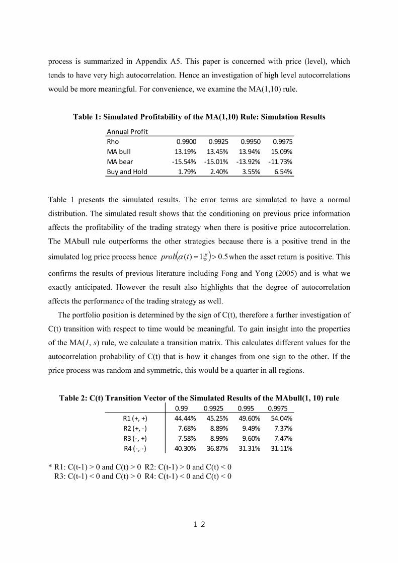
Table 1: Simulated Profitability of the MA(1,10) Rule: Simulation Results
Table 1 presents the simulated results. The error terms are simulated to have a normal
distribution. The simulated result shows that the conditioning on previous price information
affects the profitability of the trading strategy when there is positive price autocorrelation.
The MAbull rule outperforms the other strategies because there is a positive trend in the
simulated log price process hence ( ) 5.01)( >= ξα tprob when the asset return is positive. This
confirms the results of previous literature including Fong and Yong (2005) and is what we
exactly anticipated. However the result also highlights that the degree of autocorrelation
affects the performance of the trading strategy as well.
The portfolio position is determined by the sign of C(t), therefore a further investigation of
C(t) transition with respect to time would be meaningful. To gain insight into the properties
of the MA(1, s) rule, we calculate a transition matrix. This calculates different values for the
autocorrelation probability of C(t) that is how it changes from one sign to the other. If the
price process was random and symmetric, this would be a quarter in all regions.
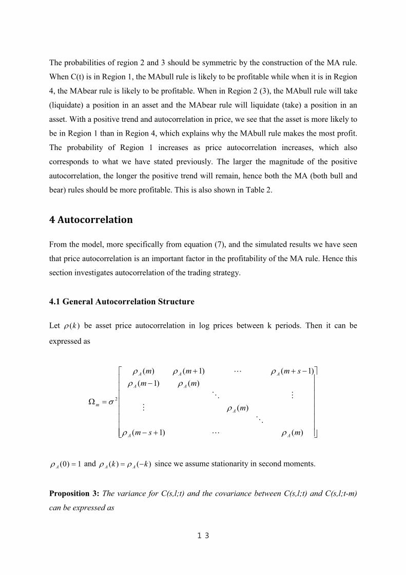
Table 2: C(t) Transition Vector of the Simulated Results of the MAbull(1, 10) rule
* R1: C(t-1) > 0 and C(t) > 0 R2: C(t-1) > 0 and C(t) < 0
R3: C(t-1) < 0 and C(t) > 0 R4: C(t-1) < 0 and C(t) < 0
Annual Profit
Rho 0.9900 0.9925 0.9950 0.9975
MA bull 13.19% 13.45% 13.94% 15.09%
MA bear -15.54% -15.01% -13.92% -11.73%
Buy and Hold 1.79% 2.40% 3.55% 6.54%
0.99 0.9925 0.995 0.9975
R1 (+, +) 44.44% 45.25% 49.60% 54.04%
R2 (+, -) 7.68% 8.89% 9.49% 7.37%
R3 (-, +) 7.58% 8.99% 9.60% 7.47%
R4 (-, -) 40.30% 36.87% 31.31% 31.11%
13
The probabilities of region 2 and 3 should be symmetric by the construction of the MA rule.
When C(t) is in Region 1, the MAbull rule is likely to be profitable while when it is in Region
4, the MAbear rule is likely to be profitable. When in Region 2 (3), the MAbull rule will take
(liquidate) a position in an asset and the MAbear rule will liquidate (take) a position in an
asset. With a positive trend and autocorrelation in price, we see that the asset is more likely to
be in Region 1 than in Region 4, which explains why the MAbull rule makes the most profit.
The probability of Region 1 increases as price autocorrelation increases, which also
corresponds to what we have stated previously. The larger the magnitude of the positive
autocorrelation, the longer the positive trend will remain, hence both the MA (both bull and
bear) rules should be more profitable. This is also shown in Table 2.
4 Autocorrelation
From the model, more specifically from equation (7), and the simulated results we have seen
that price autocorrelation is an important factor in the profitability of the MA rule. Hence this
section investigates autocorrelation of the trading strategy.
4.1 General Autocorrelation Structure
Let )(kρ be asset price autocorrelation in log prices between k periods. Then it can be
expressed as
+−
−
−++
=Ω
)()1(
)(
)()1(
)1()1()(
2
msm
m
mm
smmm
AA
A
AA
AAA
m
ρρ
ρ
ρρρρρ
σ
L
O
M
MO
L
1)0( =Aρ and )()( kk AA −= ρρ since we assume stationarity in second moments.
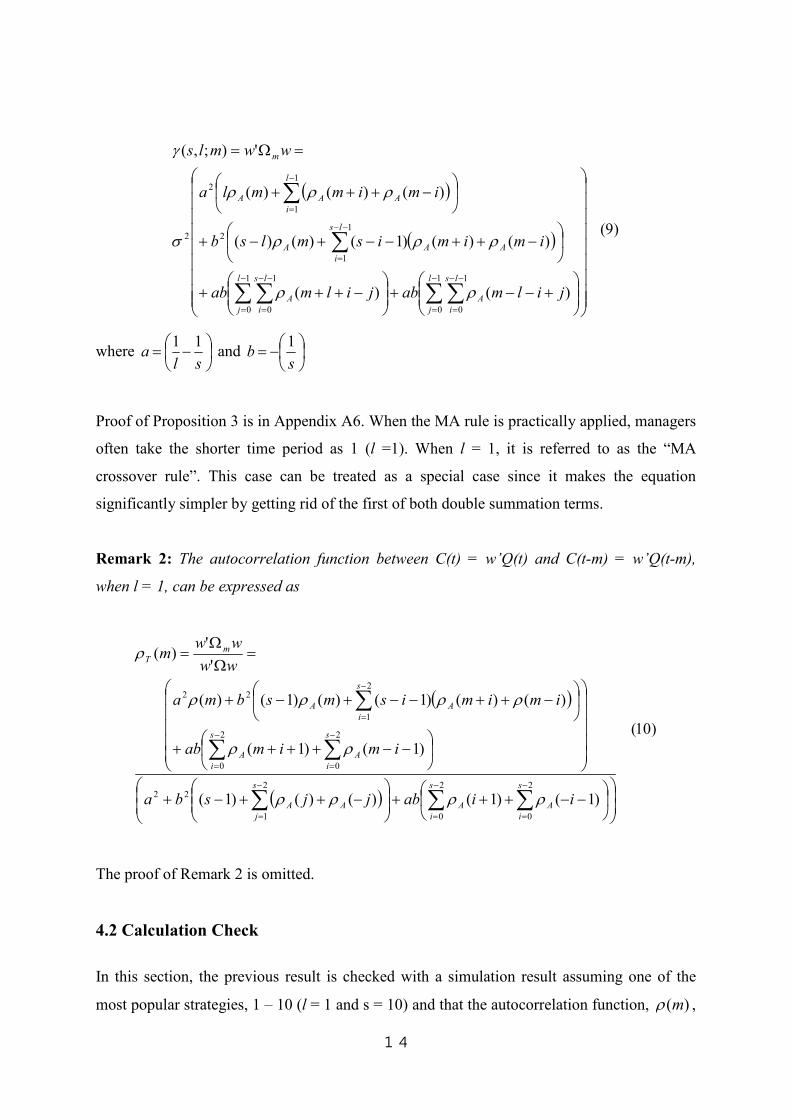
Proposition 3: The variance for C(s,l;t) and the covariance between C(s,l;t) and C(s,l;t-m)
can be expressed as
14
( )
( ))9(
)()(
)()()1()()(
)()()(
');,(
1
0
1
0
1
0
1
0
1
1
2
1
1
2
2
+−−+
−+++
−++−−+−+
−+++
=Ω=
∑∑∑∑
∑
∑
−
=
−−
=
−
=
−−
=
−−
=
−
=
l
j
ls
i
A
l
j
ls
i
A
ls
i
AAA
l
i
AAA
m
jilmabjilmab
imimismlsb
imimmla
wwmls
ρρ
ρρρ
ρρρ
σ
γ
where
−=sl
a11
and
−=s
b1
Proof of Proposition 3 is in Appendix A6. When the MA rule is practically applied, managers
often take the shorter time period as 1 (l =1). When l = 1, it is referred to as the “MA
crossover rule”. This case can be treated as a special case since it makes the equation
significantly simpler by getting rid of the first of both double summation terms.
Remark 2: The autocorrelation function between C(t) = w’Q(t) and C(t-m) = w’Q(t-m),
when l = 1, can be expressed as
( )
( )
)10(
)1()1()()()1(
)1()1(
)()()1()()1()(
'
')(
2
0
2
0
2
1
22
2
0
2
0
2
1
22
−−+++
−++−+
−−++++
−++−−+−+
=Ω
Ω=
∑∑∑
∑∑
∑
−
=
−
=
−
=
−
=
−
=
−
=
s
i
A
s
i
A
s
j
AA
s
i
A
s
i
A
s
i
AA
mT
iiabjjsba
imimab
imimismsbma
ww
wwm
ρρρρ
ρρ
ρρρρ
ρ
The proof of Remark 2 is omitted.
4.2 Calculation Check
In this section, the previous result is checked with a simulation result assuming one of the
most popular strategies, 1 – 10 (l = 1 and s = 10) and that the autocorrelation function, )(mρ ,

15
follows the AR(1) process. 2000 sets of 5000 observations of q(t) are simulated where
ttqtq ερ +−= )1()( , ( )1,0~ -ε and 95.0=ρ . LMA(t) and SMA(t) are computed from the
simulated q(t), then subtracted to get )(' tQw . The autocorrelation of )(' tQw is compared
with (4) with l = 1 and s = 10 and the percentage differences are reported.
Table 3: Simulation vs. Theoretical Result:
Autocorrelation of )(' tQw when l = 1 and s = 10
Table 3 shows that our computation is correct.
Choosing a particular MA(l,s) rule depends upon the autocorrelation properties of prices.
When s is fixed, wwΩ' is a constant. Therefore for s > l, the sensitivity of trading strategy
autocorrelation with respect to m is
Simulated AR(1) Theoretical AR(1) % Difference
wOmw[1] 0.8127 0.8131 0.0415%
wOmw[2] 0.6321 0.6325 0.0629%
wOmw[3] 0.4611 0.4619 0.1736%
wOmw[4] 0.3039 0.3051 0.3909%
wOmw[5] 0.1643 0.1658 0.9555%
wOmw[6] 0.0461 0.0479 3.8566%
wOmw[7] -0.0469 -0.0448 -4.5953%
wOmw[8] -0.1110 -0.1083 -2.4332%
wOmw[9] -0.1417 -0.1387 -2.1642%
wOmw[10] -0.1348 -0.1317 -2.3007%
wOmw[11] -0.1282 -0.1251 -2.3803%
wOmw[12] -0.1216 -0.1189 -2.2386%
wOmw[13] -0.1152 -0.1129 -1.9212%
wOmw[14] -0.1089 -0.1073 -1.5143%
wOmw[15] -0.1029 -0.1019 -0.9676%
wOmw[16] -0.0968 -0.0968 0.0307%
wOmw[17] -0.0910 -0.0920 1.1268%
wOmw[18] -0.0856 -0.0874 2.0700%
wOmw[19] -0.0808 -0.0830 2.7619%
wOmw[20] -0.0763 -0.0789 3.3288%
wOmw[21] -0.0727 -0.0749 3.0680%
wOmw[22] -0.0693 -0.0712 2.6541%
wOmw[23] -0.0661 -0.0676 2.3749%
wOmw[24] -0.0629 -0.0642 2.1334%
wOmw[25] -0.0600 -0.0610 1.7012%
wOmw[26] -0.0573 -0.0580 1.1180%
wOmw[27] -0.0546 -0.0551 0.8748%
wOmw[28] -0.0518 -0.0523 0.9222%
wOmw[29] -0.0491 -0.0497 1.2625%
wOmw[30] -0.0466 -0.0472 1.3013%

16
( )
∂
−−∂+
∂++∂
+
∂
−∂+
∂+∂
−−+∂
∂−+
=∂Ω∂
=∂
∂
∑
∑−
=
−
=
2
0
2
1
222
)1()1(
))()(
)1()(
)1(')(
s
i
AA
s
i
AAA
mT
m
im
m
imab
m
im
m
imisb
m
msba
m
ww
m
m
ρρ
ρρρ
ρ
If 0)(<
∂∂
m
mAρ , we have 0)(<
∂∂
m
mTρ
It may well be reasonable to design optimal properties. We do not pursue this further but
instead look at the links between the Autocorrelation Function (ACF) of the MA rule and
some simple time series models.
In the next two sections, the autocorrelation structure of the 1 – 10 strategy is investigated.
Equation (9) is computed m = 30 and Aρ incrementing from 0.05 to 0.95 with an interval of
0.05.
4.3 When ACF follows AR(1)
(Insert Table 4)
(Insert Figure 1)
4.4 When ACF follows MA(1)
(Insert Table 5)
(Insert Figure 2)
Since the tables and figures are too large to fit here, they have been placed on the following
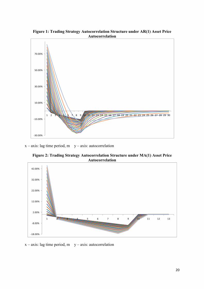
pages. The autocorrelation of the 1 – 10 strategy becomes 0 for m > 10.
4.5 The MA(l,s) vs. Price Autocorrelation
17
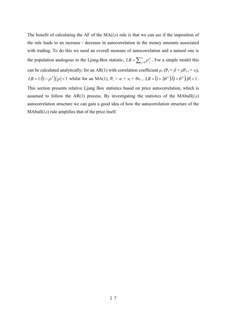
The benefit of calculating the AF of the MA(l,s) rule is that we can see if the imposition of
the rule leads to an increase / decrease in autocorrelation in the money amounts associated
with trading. To do this we need an overall measure of autocorrelation and a natural one is
the population analogous to the Ljung-Box statistic, ∑∞
==
0
2
j jLB ρ . For a simple model this
can be calculated analytically; for an AR(1) with correlation coefficient ρ, (Pt = β + ρPt-1 + νt),
( ) 1 ;1/1 2 <−= ρρLB whilst for an MA(1), Pt = α + νt + θνt , ( ) ( ) 1 ;1/21 22 <++= θθθLB .
This section presents relative Ljung Box statistics based on price autocorrelation, which is
assumed to follow the AR(1) process. By investigating the statistics of the MAbull(l,s)
autocorrelation structure we can gain a good idea of how the autocorrelation structure of the
MAbull(l,s) rule amplifies that of the price itself.

18
Table 4: The MA(1,10) Rule Autocorrelation Structure under AR(1) Asset Price Autocorrelation, Aρ increases from 0.05 to 0.95 and
m = 30
0.05 0.1 0.15 0.2 0.25 0.3 0.35 0.4 0.45 0.5 0.55 0.6 0.65 0.7 0.75 0.8 0.85 0.9 0.95
1 3.77% 8.64% 13.49% 18.32% 23.13% 27.91% 32.65% 37.35% 41.98% 46.55% 51.03% 55.40% 59.63% 63.72% 67.64% 71.36% 74.89% 78.20% 81.31%
2 -2.21% -1.72% -0.77% 0.64% 2.51% 4.82% 7.55% 10.70% 14.23% 18.12% 22.34% 26.85% 31.61% 36.58% 41.72% 46.98% 52.34% 57.77% 63.25%
3 -3.68% -3.99% -4.19% -4.23% -4.05% -3.57% -2.75% -1.54% 0.11% 2.24% 4.87% 8.04% 11.76% 16.05% 20.90% 26.34% 32.36% 38.97% 46.19%
4 -4.92% -5.44% -5.99% -6.55% -7.09% -7.55% -7.87% -7.99% -7.83% -7.30% -6.31% -4.76% -2.55% 0.42% 4.26% 9.09% 14.99% 22.10% 30.51%
5 -6.15% -6.81% -7.54% -8.36% -9.24% -10.18% -11.13% -12.06% -12.88% -13.51% -13.82% -13.68% -12.92% -11.35% -8.77% -4.94% 0.38% 7.46% 16.58%
6 -7.38% -8.17% -9.05% -10.04% -11.14% -12.34% -13.65% -15.02% -16.42% -17.76% -18.94% -19.82% -20.20% -19.84% -18.48% -15.76% -11.29% -4.62% 4.79%
7 -8.61% -9.52% -10.53% -11.63% -12.84% -14.17% -15.61% -17.15% -18.77% -20.43% -22.05% -23.51% -24.64% -25.19% -24.86% -23.22% -19.74% -13.77% -4.48%
8 -9.81% -10.77% -11.78% -12.85% -13.99% -15.22% -16.54% -17.96% -19.49% -21.11% -22.79% -24.46% -25.97% -27.13% -27.62% -26.99% -24.59% -19.59% -10.83%
9 -10.48% -11.00% -11.59% -12.24% -12.97% -13.79% -14.73% -15.80% -17.02% -18.40% -19.95% -21.63% -23.36% -24.97% -26.20% -26.57% -25.40% -21.65% -13.87%
10 -0.52% -1.10% -1.74% -2.45% -3.24% -4.14% -5.15% -6.32% -7.66% -9.20% -10.97% -12.98% -15.18% -17.48% -19.65% -21.26% -21.59% -19.49% -13.17%
11 -0.03% -0.11% -0.26% -0.49% -0.81% -1.24% -1.80% -2.53% -3.45% -4.60% -6.03% -7.79% -9.87% -12.24% -14.74% -17.01% -18.35% -17.54% -12.51%
12 0.00% -0.01% -0.04% -0.10% -0.20% -0.37% -0.63% -1.01% -1.55% -2.30% -3.32% -4.67% -6.41% -8.57% -11.05% -13.60% -15.60% -15.78% -11.89%
13 0.00% 0.00% -0.01% -0.02% -0.05% -0.11% -0.22% -0.40% -0.70% -1.15% -1.83% -2.80% -4.17% -6.00% -8.29% -10.88% -13.26% -14.21% -11.29%
14 0.00% 0.00% 0.00% 0.00% -0.01% -0.03% -0.08% -0.16% -0.31% -0.58% -1.00% -1.68% -2.71% -4.20% -6.22% -8.71% -11.27% -12.79% -10.73%
15 0.00% 0.00% 0.00% 0.00% 0.00% -0.01% -0.03% -0.06% -0.14% -0.29% -0.55% -1.01% -1.76% -2.94% -4.66% -6.97% -9.58% -11.51% -10.19%
16 0.00% 0.00% 0.00% 0.00% 0.00% 0.00% -0.01% -0.03% -0.06% -0.14% -0.30% -0.61% -1.14% -2.06% -3.50% -5.57% -8.14% -10.36% -9.68%
17 0.00% 0.00% 0.00% 0.00% 0.00% 0.00% 0.00% -0.01% -0.03% -0.07% -0.17% -0.36% -0.74% -1.44% -2.62% -4.46% -6.92% -9.32% -9.20%
18 0.00% 0.00% 0.00% 0.00% 0.00% 0.00% 0.00% 0.00% -0.01% -0.04% -0.09% -0.22% -0.48% -1.01% -1.97% -3.57% -5.88% -8.39% -8.74%
19 0.00% 0.00% 0.00% 0.00% 0.00% 0.00% 0.00% 0.00% -0.01% -0.02% -0.05% -0.13% -0.31% -0.71% -1.48% -2.85% -5.00% -7.55% -8.30%
20 0.00% 0.00% 0.00% 0.00% 0.00% 0.00% 0.00% 0.00% 0.00% -0.01% -0.03% -0.08% -0.20% -0.49% -1.11% -2.28% -4.25% -6.79% -7.89%
21 0.00% 0.00% 0.00% 0.00% 0.00% 0.00% 0.00% 0.00% 0.00% 0.00% -0.02% -0.05% -0.13% -0.35% -0.83% -1.83% -3.61% -6.12% -7.49%
22 0.00% 0.00% 0.00% 0.00% 0.00% 0.00% 0.00% 0.00% 0.00% 0.00% -0.01% -0.03% -0.09% -0.24% -0.62% -1.46% -3.07% -5.50% -7.12%
23 0.00% 0.00% 0.00% 0.00% 0.00% 0.00% 0.00% 0.00% 0.00% 0.00% 0.00% -0.02% -0.06% -0.17% -0.47% -1.17% -2.61% -4.95% -6.76%
24 0.00% 0.00% 0.00% 0.00% 0.00% 0.00% 0.00% 0.00% 0.00% 0.00% 0.00% -0.01% -0.04% -0.12% -0.35% -0.93% -2.22% -4.46% -6.42%
25 0.00% 0.00% 0.00% 0.00% 0.00% 0.00% 0.00% 0.00% 0.00% 0.00% 0.00% -0.01% -0.02% -0.08% -0.26% -0.75% -1.89% -4.01% -6.10%
26 0.00% 0.00% 0.00% 0.00% 0.00% 0.00% 0.00% 0.00% 0.00% 0.00% 0.00% 0.00% -0.02% -0.06% -0.20% -0.60% -1.60% -3.61% -5.80%
27 0.00% 0.00% 0.00% 0.00% 0.00% 0.00% 0.00% 0.00% 0.00% 0.00% 0.00% 0.00% -0.01% -0.04% -0.15% -0.48% -1.36% -3.25% -5.51%
28 0.00% 0.00% 0.00% 0.00% 0.00% 0.00% 0.00% 0.00% 0.00% 0.00% 0.00% 0.00% -0.01% -0.03% -0.11% -0.38% -1.16% -2.92% -5.23%
29 0.00% 0.00% 0.00% 0.00% 0.00% 0.00% 0.00% 0.00% 0.00% 0.00% 0.00% 0.00% 0.00% -0.02% -0.08% -0.31% -0.98% -2.63% -4.97%
30 0.00% 0.00% 0.00% 0.00% 0.00% 0.00% 0.00% 0.00% 0.00% 0.00% 0.00% 0.00% 0.00% -0.01% -0.06% -0.25% -0.84% -2.37% -4.72%

19
Table 5: The MA(1,10) Rule Autocorrelation Structure under MA(1) Asset Price Autocorrelation, Aρ increases from 0.05 to 0.95 and
m = 30
0.05 0.1 0.15 0.2 0.25 0.3 0.35 0.4 0.45 0.5 0.55 0.6 0.65 0.7 0.75 0.8 0.85 0.9 0.95
1 -0.87% -0.14% 1.04% 2.65% 4.65% 6.98% 9.58% 12.41% 15.41% 18.53% 21.71% 24.92% 28.12% 31.27% 34.36% 37.37% 40.28% 43.07% 45.75%
2 -2.23% -2.27% -2.32% -2.40% -2.49% -2.59% -2.71% -2.84% -2.98% -3.13% -3.27% -3.42% -3.57% -3.71% -3.85% -3.99% -4.12% -4.25% -4.38%
3 -3.35% -3.40% -3.48% -3.59% -3.73% -3.89% -4.07% -4.27% -4.47% -4.69% -4.91% -5.13% -5.35% -5.57% -5.78% -5.99% -6.19% -6.38% -6.57%
4 -4.47% -4.53% -4.64% -4.79% -4.97% -5.19% -5.43% -5.69% -5.96% -6.25% -6.54% -6.84% -7.13% -7.42% -7.71% -7.98% -8.25% -8.51% -8.75%
5 -5.58% -5.67% -5.80% -5.99% -6.22% -6.48% -6.78% -7.11% -7.45% -7.81% -8.18% -8.55% -8.91% -9.28% -9.63% -9.98% -10.31% -10.63% -10.94%
6 -6.70% -6.80% -6.96% -7.19% -7.46% -7.78% -8.14% -8.53% -8.95% -9.38% -9.81% -10.26% -10.70% -11.13% -11.56% -11.97% -12.37% -12.76% -13.13%
7 -7.82% -7.93% -8.12% -8.38% -8.70% -9.08% -9.50% -9.95% -10.44% -10.94% -11.45% -11.97% -12.48% -12.99% -13.49% -13.97% -14.44% -14.89% -15.32%
8 -8.93% -9.07% -9.28% -9.58% -9.95% -10.38% -10.86% -11.38% -11.93% -12.50% -13.09% -13.68% -14.26% -14.84% -15.41% -15.97% -16.50% -17.01% -17.51%
9 -10.02% -10.09% -10.20% -10.35% -10.54% -10.75% -11.00% -11.26% -11.54% -11.83% -12.13% -12.43% -12.72% -13.02% -13.31% -13.59% -13.86% -14.12% -14.37%
10 -0.02% -0.10% -0.22% -0.38% -0.59% -0.83% -1.09% -1.38% -1.69% -2.01% -2.33% -2.66% -2.99% -3.31% -3.63% -3.94% -4.23% -4.52% -4.79%
11 0.00% 0.00% 0.00% 0.00% 0.00% 0.00% 0.00% 0.00% 0.00% 0.00% 0.00% 0.00% 0.00% 0.00% 0.00% 0.00% 0.00% 0.00% 0.00%
12 0.00% 0.00% 0.00% 0.00% 0.00% 0.00% 0.00% 0.00% 0.00% 0.00% 0.00% 0.00% 0.00% 0.00% 0.00% 0.00% 0.00% 0.00% 0.00%
13 0.00% 0.00% 0.00% 0.00% 0.00% 0.00% 0.00% 0.00% 0.00% 0.00% 0.00% 0.00% 0.00% 0.00% 0.00% 0.00% 0.00% 0.00% 0.00%
20
Figure 1: Trading Strategy Autocorrelation Structure under AR(1) Asset Price
Autocorrelation
x – axis: lag time period, m y – axis: autocorrelation
Figure 2: Trading Strategy Autocorrelation Structure under MA(1) Asset Price
Autocorrelation
x – axis: lag time period, m y – axis: autocorrelation
-30.00%
-10.00%
10.00%
30.00%
50.00%
70.00%
1 2 3 4 5 6 7 8 9 10 11 12 13 14 15 16 17 18 19 20 21 22 23 24 25 26 27 28 29 30
-18.00%
-8.00%
2.00%
12.00%
22.00%
32.00%
42.00%
1 2 3 4 5 6 7 8 9 10 11 12 13
21
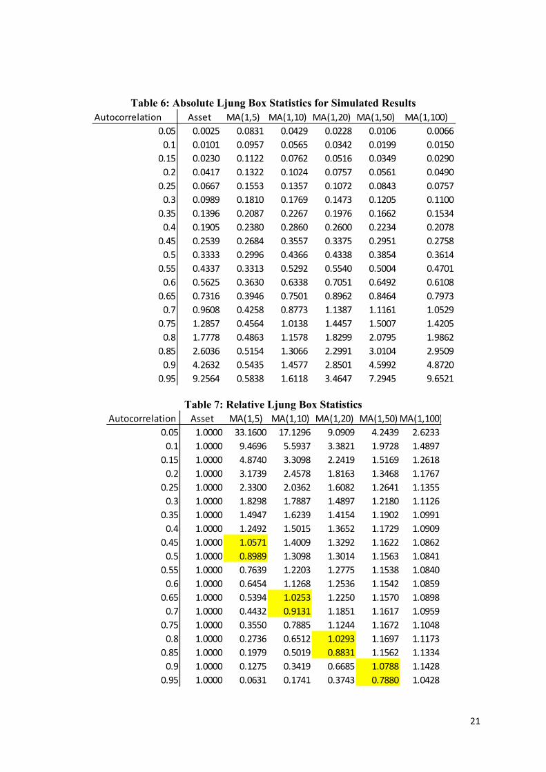
Table 6: Absolute Ljung Box Statistics for Simulated Results
Table 7: Relative Ljung Box Statistics
Autocorrelation Asset MA(1,5) MA(1,10) MA(1,20) MA(1,50) MA(1,100)
0.05 0.0025 0.0831 0.0429 0.0228 0.0106 0.0066
0.1 0.0101 0.0957 0.0565 0.0342 0.0199 0.0150
0.15 0.0230 0.1122 0.0762 0.0516 0.0349 0.0290
0.2 0.0417 0.1322 0.1024 0.0757 0.0561 0.0490
0.25 0.0667 0.1553 0.1357 0.1072 0.0843 0.0757
0.3 0.0989 0.1810 0.1769 0.1473 0.1205 0.1100
0.35 0.1396 0.2087 0.2267 0.1976 0.1662 0.1534
0.4 0.1905 0.2380 0.2860 0.2600 0.2234 0.2078
0.45 0.2539 0.2684 0.3557 0.3375 0.2951 0.2758
0.5 0.3333 0.2996 0.4366 0.4338 0.3854 0.3614
0.55 0.4337 0.3313 0.5292 0.5540 0.5004 0.4701
0.6 0.5625 0.3630 0.6338 0.7051 0.6492 0.6108
0.65 0.7316 0.3946 0.7501 0.8962 0.8464 0.7973
0.7 0.9608 0.4258 0.8773 1.1387 1.1161 1.0529
0.75 1.2857 0.4564 1.0138 1.4457 1.5007 1.4205
0.8 1.7778 0.4863 1.1578 1.8299 2.0795 1.9862
0.85 2.6036 0.5154 1.3066 2.2991 3.0104 2.9509
0.9 4.2632 0.5435 1.4577 2.8501 4.5992 4.8720
0.95 9.2564 0.5838 1.6118 3.4647 7.2945 9.6521
Autocorrelation Asset MA(1,5) MA(1,10) MA(1,20) MA(1,50) MA(1,100)
0.05 1.0000 33.1600 17.1296 9.0909 4.2439 2.6233
0.1 1.0000 9.4696 5.5937 3.3821 1.9728 1.4897
0.15 1.0000 4.8740 3.3098 2.2419 1.5169 1.2618
0.2 1.0000 3.1739 2.4578 1.8163 1.3468 1.1767
0.25 1.0000 2.3300 2.0362 1.6082 1.2641 1.1355
0.3 1.0000 1.8298 1.7887 1.4897 1.2180 1.1126
0.35 1.0000 1.4947 1.6239 1.4154 1.1902 1.0991
0.4 1.0000 1.2492 1.5015 1.3652 1.1729 1.0909
0.45 1.0000 1.0571 1.4009 1.3292 1.1622 1.0862
0.5 1.0000 0.8989 1.3098 1.3014 1.1563 1.0841
0.55 1.0000 0.7639 1.2203 1.2775 1.1538 1.0840
0.6 1.0000 0.6454 1.1268 1.2536 1.1542 1.0859
0.65 1.0000 0.5394 1.0253 1.2250 1.1570 1.0898
0.7 1.0000 0.4432 0.9131 1.1851 1.1617 1.0959
0.75 1.0000 0.3550 0.7885 1.1244 1.1672 1.1048
0.8 1.0000 0.2736 0.6512 1.0293 1.1697 1.1173
0.85 1.0000 0.1979 0.5019 0.8831 1.1562 1.1334
0.9 1.0000 0.1275 0.3419 0.6685 1.0788 1.1428
0.95 1.0000 0.0631 0.1741 0.3743 0.7880 1.0428
22
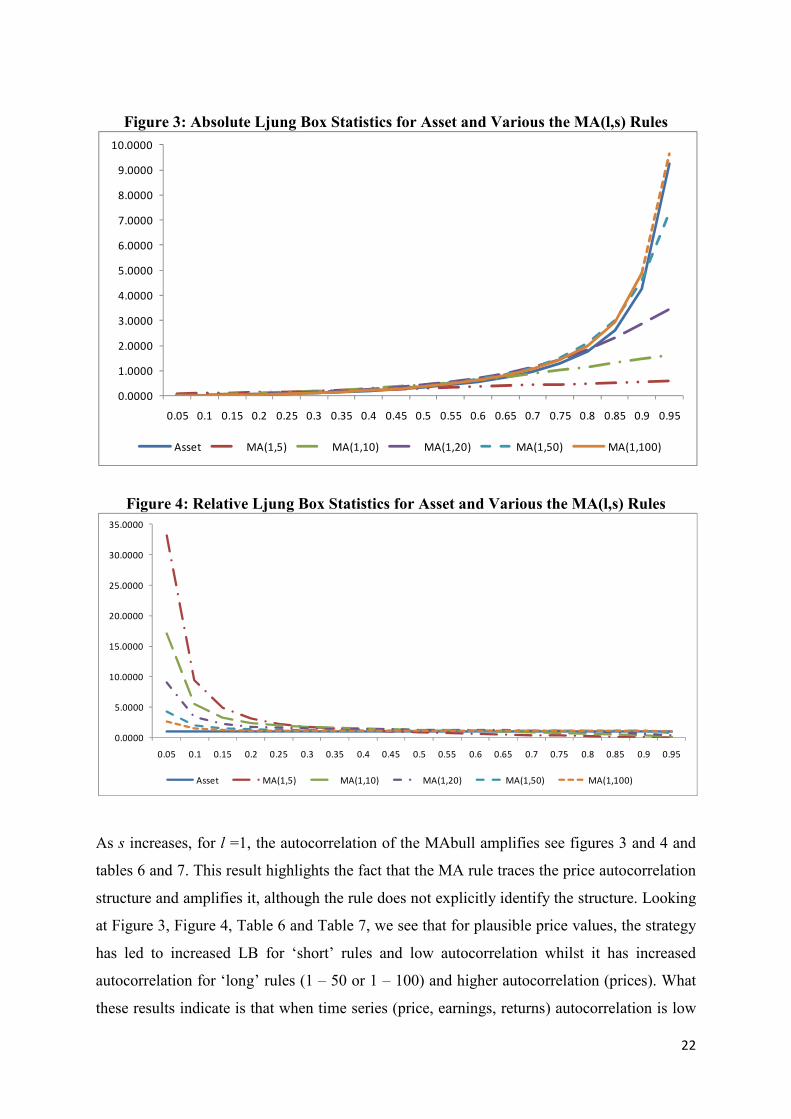
Figure 3: Absolute Ljung Box Statistics for Asset and Various the MA(l,s) Rules
Figure 4: Relative Ljung Box Statistics for Asset and Various the MA(l,s) Rules
As s increases, for l =1, the autocorrelation of the MAbull amplifies see figures 3 and 4 and
tables 6 and 7. This result highlights the fact that the MA rule traces the price autocorrelation
structure and amplifies it, although the rule does not explicitly identify the structure. Looking
at Figure 3, Figure 4, Table 6 and Table 7, we see that for plausible price values, the strategy
has led to increased LB for ‘short’ rules and low autocorrelation whilst it has increased
autocorrelation for ‘long’ rules (1 – 50 or 1 – 100) and higher autocorrelation (prices). What
these results indicate is that when time series (price, earnings, returns) autocorrelation is low
0.0000
1.0000
2.0000
3.0000
4.0000
5.0000
6.0000
7.0000
8.0000
9.0000
10.0000
0.05 0.1 0.15 0.2 0.25 0.3 0.35 0.4 0.45 0.5 0.55 0.6 0.65 0.7 0.75 0.8 0.85 0.9 0.95
Asset MA(1,5) MA(1,10) MA(1,20) MA(1,50) MA(1,100)
0.0000
5.0000
10.0000
15.0000
20.0000
25.0000
30.0000
35.0000
0.05 0.1 0.15 0.2 0.25 0.3 0.35 0.4 0.45 0.5 0.55 0.6 0.65 0.7 0.75 0.8 0.85 0.9 0.95
Asset MA(1,5) MA(1,10) MA(1,20) MA(1,50) MA(1,100)

23
an MA rule with a small s should be used whilst an MA rule with a large s should be used
with a highly autocorrelated process. As we discussed earlier, the application of our current
model is not necessarily restricted to the price process. Based on our results in this section,
when the MA rule is employed with a price MA, where price autocorrelation is very high, an
MA rule with a large s would be appropriate. And when the MA rule is applied to a return
process, which has lower autocorrelation than the price process in general, a smaller s would
be suitable.
5 Empirical Evidence
The previous section has focused on analyzing how the MA rule identifies the price
autocorrelation structure and amplifies it in a simulated setting where we know the actual
price autocorrelation structure. It would be meaningful to apply the MA rule to real historical
data.
Table 8: Detrended Log Price First Order Autocorrelation and Trends of International
Indices
* Sample date from January 4, 2000 to June 1, 2011
In Table 8 we see a very high first order autocorrelation in detrended log price process in
major indices: We employ Dickey Fuller tests to see whether a unit root is present
Table 9: Price trend, Dickey Fuller Test and the Profitability of the MA(1,10) Rule
Applied to Various Indies. Historical Daily Data from Jan 4, 2000 to May 31, 2011
* Dickey Fuller critical value: -2.58 at 1% and -1.95 at 5%
Kospi Hang Seng Jakarta S&P500 FTSE100 Nikke
Rho 0.9995 0.9962 0.9961 0.9961 0.9960 0.9972
Trend 0.046% 0.025% 0.088% -0.001% 0.001% -0.007%
Kospi Hang Seng Jakarta S&P500 FTSE100 Nikke
Mu 0.00046 0.00025 0.00088 -0.00001 0.00001 -0.00007
Rho 0.9955 0.9971 0.9980 0.9966 0.9967 0.9976
DF Test Stat -3.71 -2.59 -3.15 -2.43 -2.51 -2.13
MA bull 7.30% 6.29% 13.25% -4.02% -4.10% -2.38%
MA bear -2.28% -2.73% -6.30% 4.68% 4.71% -1.34%
Buy and Hold 5.25% 3.13% 9.66% -0.90% -0.97% -4.76%
24
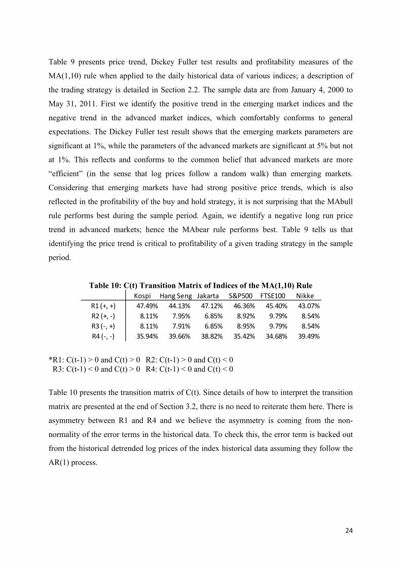
Table 9 presents price trend, Dickey Fuller test results and profitability measures of the
MA(1,10) rule when applied to the daily historical data of various indices; a description of
the trading strategy is detailed in Section 2.2. The sample data are from January 4, 2000 to
May 31, 2011. First we identify the positive trend in the emerging market indices and the
negative trend in the advanced market indices, which comfortably conforms to general
expectations. The Dickey Fuller test result shows that the emerging markets parameters are
significant at 1%, while the parameters of the advanced markets are significant at 5% but not
at 1%. This reflects and conforms to the common belief that advanced markets are more
“efficient” (in the sense that log prices follow a random walk) than emerging markets.
Considering that emerging markets have had strong positive price trends, which is also
reflected in the profitability of the buy and hold strategy, it is not surprising that the MAbull
rule performs best during the sample period. Again, we identify a negative long run price
trend in advanced markets; hence the MAbear rule performs best. Table 9 tells us that
identifying the price trend is critical to profitability of a given trading strategy in the sample
period.
Table 10: C(t) Transition Matrix of Indices of the MA(1,10) Rule
*R1: C(t-1) > 0 and C(t) > 0 R2: C(t-1) > 0 and C(t) < 0
R3: C(t-1) < 0 and C(t) > 0 R4: C(t-1) < 0 and C(t) < 0
Table 10 presents the transition matrix of C(t). Since details of how to interpret the transition
matrix are presented at the end of Section 3.2, there is no need to reiterate them here. There is
asymmetry between R1 and R4 and we believe the asymmetry is coming from the non-
normality of the error terms in the historical data. To check this, the error term is backed out
from the historical detrended log prices of the index historical data assuming they follow the
AR(1) process.
Kospi Hang Seng Jakarta S&P500 FTSE100 Nikke
R1 (+, +) 47.49% 44.13% 47.12% 46.36% 45.40% 43.07%
R2 (+, -) 8.11% 7.95% 6.85% 8.92% 9.79% 8.54%
R3 (-, +) 8.11% 7.91% 6.85% 8.95% 9.79% 8.54%
R4 (-, -) 35.94% 39.66% 38.82% 35.42% 34.68% 39.49%
25
Table 11: Error Term Statistics
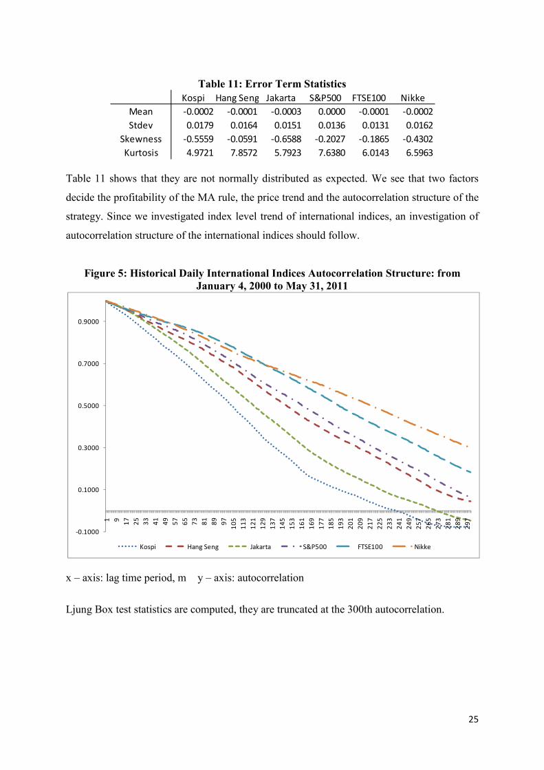
Table 11 shows that they are not normally distributed as expected. We see that two factors
decide the profitability of the MA rule, the price trend and the autocorrelation structure of the
strategy. Since we investigated index level trend of international indices, an investigation of
autocorrelation structure of the international indices should follow.
Figure 5: Historical Daily International Indices Autocorrelation Structure: from
January 4, 2000 to May 31, 2011
x – axis: lag time period, m y – axis: autocorrelation
Ljung Box test statistics are computed, they are truncated at the 300th autocorrelation.
Kospi Hang Seng Jakarta S&P500 FTSE100 Nikke
Mean -0.0002 -0.0001 -0.0003 0.0000 -0.0001 -0.0002
Stdev 0.0179 0.0164 0.0151 0.0136 0.0131 0.0162
Skewness -0.5559 -0.0591 -0.6588 -0.2027 -0.1865 -0.4302
Kurtosis 4.9721 7.8572 5.7923 7.6380 6.0143 6.5963
-0.1000
0.1000
0.3000
0.5000
0.7000
0.9000
1 9
17
25
33
41
49
57
65
73
81
89
97
10
5
11
3
12
1
12
9
13
7
14
5
15
3
16
1
16
9
17
7
18
5
19
3
20
1
20
9
21
7
22
5
23
3
24
1
24
9
25
7
26
5
27
3
28
1
28
9
29
7
Kospi Hang Seng Jakarta S&P500 FTSE100 Nikke

26
Table 12: Ljung-Box Test Statistics for Indices (Prices) and the MA(1,250) Strategy
from January 4, 2000 to May 31, 2011
Table 13: Ljung-Box Test Statistics for Indices (Returns) and the MA(1,10) Strategy
from January 4, 2000 to May 31, 2011
Table 14: Simulated Ljung-Box Test Statistics for the AR(1) Model
Table 12 presents the LB statistics for international indices price and the MA(1,250) strategy,
and Table 13 presents the LB statistics for international indices returns and the MA(1,10)
strategy. The number in Table 12 may look very high compared to previous simulated results
of trading strategy autocorrelations below 0.95. Hence, the LB statistics of an asset when it
follows the AR(1) process with a very high ρ are presented in 14 to confirm the
reasonableness of the numbers in Table 12. We have seen that when the price autocorrelation
is very high, a strategy with a large s becomes effective. In this empirical test of index price
series, we will use 1 year MA, hence the MA(1, 250) rule. 250 days were chosen for no
specific reason but to ensure large enough s. We could have used (1, 100) or (1, 500) and the
result would be the same. We also argued that when ρ is very low, a strategy with small s is
effective. Hence for index return series we will use the MA(1, 10) rule, although any small s
would have equivalent results. The result clearly shows that the MA strategy amplifies the
level of autocorrelation in the index level.
6 Conclusion
This paper first presents a technical definition of momentum in order to investigate how
technical analysis, especially the MA rule, becomes profitable and theoretically demonstrates
that the trading rule is profitable. The theoretical examination revealed that, in addition, price
Kospi Hang Seng Jakarta S&P500 FTSE100 Nikke
1st order Autocorrel 0.9955 0.9971 0.9980 0.9966 0.9967 0.9976
log Price LB 70.22 103.57 85.26 112.08 133.02 141.40
MA(1,250) LB 127.22 137.52 127.57 147.73 160.46 182.01
Kospi Hang Seng Jakarta S&P500 FTSE100 Nikke
1st order Autocorrel 0.0155 -0.0216 0.1209 -0.0852 -0.0628 -0.0310
log Price LB 0.1404 0.2041 0.1589 0.1654 0.1897 0.1424
MA(1,10) LB 0.2087 0.2919 0.1884 0.1871 0.2189 0.1627
Asset rho 0.99 0.9925 0.995 0.9975
LB 49.25 65.92 99.25 199.25
27
autocorrelation might be another fundamental reason for profitability, and the further
investigation of the autocorrelation structure of the MA rule showed that the MA rule reflects
the price autocorrelation structure, without identifying it. This analysis sheds some light on
why analysts use technical trading rules. There are three main findings in this paper:
1. The MA rule identifies and takes advantage of price trend
2. 2. The MA rule is a simple and straightforward way of exploiting price
autocorrelation without actually knowing it
3. 3. In the case of MA(1, s) rules, where s is a time period for the short position’s
MA, the amplification of the autocorrelation structure is more prominent for a
small s when the level of autocorrelation is low and for a large s, when the level of
autocorrelation is high
The first finding is already well known and discussed in the earlier literature. We confirm it
by constructing a simple model with a single asset. The second finding has not been
investigated in the previous literature due to lack of a precise technical definition of
momentum. We show this with simulated results and empirical data from 6 international
indices from developing and mature markets. The third finding suggests what length of s
should be applied in employing the MA rule.
These findings should be considered important in themselves since they identify why the
MA rule is used. However, the practical application of this is also interesting. One of many
natural questions that can be asked is how well would the MA rule would perform if the full
price autocorrelation structure was known. After all, we saw that the MA rule is all about
simplification of conditioning on the past price information. Therefore, if we use the entire
past price information, this should outperform the MA rule. However, in practice the tradeoff
between the inefficiency and the cost of knowing the full autocorrelation would justify the
use of the MA rule. Nevertheless the extent of the efficiency gain would be a worthy area for
future research.

28
Reference
Achelis, S. (2000): “Technical Analysis from A to Z”, 2nd Edition, McGraw-Hill Companies
Allen, F. and R. Karjalainen. (1999): “Using Genetic Algorithms to Find Technical Trading
Rules.” Journal of Financial Economics 51, 245–271.
Blume, L., Easley, D. and O'Hara, M. B. (1994): “Market Statistics and Technical Analysis:
The Role of Volume.” Journal of Finance 49, 153–181.
Brock, W., Lakonishok, J., and LeBaron, B. (1992): “Simple Technical Trading Rules and
the Stochastic Properties of Stock Returns”, The Journal of Finance, Vol. 47, No. 5,
December 1992, pp. 1731 – 1764.
Brown, S. J., W. N. Goetzmann, and A. Kumar. (1998): “The Dow Theory: William Peter
Hamilton’s Track Record Reconsidered.” Journal of Finance 53, 1311–1333.
Carhart, M.M. (1997): “On persistence in mutual fund performance”, Journal of Finance 52,
57-82.
Chan, K., Hameed, A. and Tong, W. (2000): “Profitability of Momentum Strategies in the
International Equity Markets.” Journal of Financial and Quantitative Analysis 35, 153–172.
Chan, K., Jegadeesh, N. and Lakonishok, J. (1996): “Momentum Strategies”, Journal of
Finance, Vol. 51 No. 5.
Chang, P. H. K. and Osler, C. L. (1999): “Methodological Madness: Technical Analysis and
the Irrationality of Exchange-Rate Forecasts.” Economic Journal 109, 636–661.
Fama, E.F. and French, K.R. (1996): “Multifactor explanations of asset pricing anomalies”,
Journal of Finance 51, 55-84.
Fong, W. M. and Yong, H. M. (2005): “Chasing trends: recursive moving average trading
rules and internet stocks”, Journal of Empirical Finance, Volume 12, Issue 1, January 2005,
Pages 43-76.
Gencay, R. (1996): “Non-Linear Prediction of Security Returns with Moving Average Rules”,
Journal of Forecasting 15, 165–174.
Gencay, R. (1998): “The Predictability of Security Returns with Simple Technical Trading
Rules.” Journal of Empirical Finance 5, 347–359.
Gencay, R. (1999): “Linear, Non-Linear and Essential Foreign Exchange Rate Prediction
with Simple Technical Trading Rules”, Journal of International Economics 47, 91– 107.
Gunasekarage, A. and Power, D.M. (2000): “The profitability of moving average trading
rules in South Asian stock markets”, Emerging Markets Review 2 (2001) 17-33.
29
Hudson, R., Dempsey, M. and Keasey, K. (1996): “A note on the weak form efficiency of
capital markets: the application of simple technical trading rules to UK stock prices - 1935 to
1994”, Journal of Banking and Finance 20, 1121-1132.
Jegadeesh N. and Titman S. (1993): “Returns to buying winners and selling losers:
Implications for stock market efficiency”, Journal of Finance 48, 65–91.
Jegadeesh N. and Titman S. (2001): “Profitability of momentum strategies: an evaluation of
alternative explanations”, Journal of Finance 56:699–720.
Lo, A. W., H. Mamaysky, and J. Wang. (2000): “Foundations of Technical Analysis:
Computational Algorithms, Statistical Inference, and Empirical Implementation.” Journal of
Finance 55, 1705–1765.
Neely, C. J. and Weller. P. (1999): “Technical Trading Rules in the European Monetary
System.” Journal of International Money and Finance 18, 429–458
Neely, C. J., Weller, P. and Dittmar, R. (1997): “Is Technical Analysis in the Foreign
Exchange Market Profitable? A Genetic Programming Approach.” Journal of Financial and
Quantitative Analysis 32, 405–426.
Reitz, S., (2006): “On the predictive content of technical analysis”, The North American
Journal of Economics and Finance, 17(2), 121-137.
Rouwenhorst, K. G. (1998): “International Momentum Strategies”, Journal of Finance, Vol.
53, No. 1, pp. 267-284.
Schwager, J. D. (1992) The New Market Wizards: Conversations With America's Top
Traders. John Wiley and Sons, (pg. 224)
Shleifer, A. (2000): “Inefficient Markets”, Oxford University Press.
Sweeney, R. J. (1986): “Beating the Foreign Exchange Market.” Journal of Finance 41, 163–
182.
Sweeney, R. J. (1988): “Some New Filter Rule Tests: Methods and Results.” Journal of
Financial and Quantitative Analysis 23, 285–300.

30
Appendix
A1 Proof of Proposition 1
The ratio of future price in period h to today’s price can be represented as
( ) ( ) ( )hudWttPtP
htP ht
t
h µµθσθ exp)((expexp)()(
)( 1)exp(
−−=
+∫
+−−
Hence the expected value of this is
( ) ( )hhtP
tP
htPE h µ
θθ
σθ exp1)2exp(
4
1exp)(
)(
)( 21)exp(
−=
+ −−
This can be thought of as the population momentum measure conditioned on time t. Taking
logs, we get
( ) hh
tPhtP
htPE µ
θθ
σθ +−
+−−=
+ 1)2exp(
4
1)(ln1)exp(
)(
)(ln 2
Therefore we have
1)exp()(ln
)(
)(ln
−−=∂
+∂
θhtP
tP
htPE
A2 Derivation of Definition 2
( ))('exp)1(
)1(11
exp
)1()1(
exp
)1(
exp
)1(
exp)(
11
11
11
tQws
itqitq
sl
s
itq
l
itq
s
itq
l
itq
tC
s
i
l
i
s
i
l
i
s
i
l
i
=
+−++−
−=
+−
−+−
=
+−
+−
=
∑∑
∑∑
∑∑
==
==
==
A3 Derivation of Lemma 1
31
( )( )( ) ( )( )
m
jtjtP
ttP
m
j
∑−
=
−−−
>−
1
0
log
)(log
µµ
( )( )( )
m
j
m
jtP
tP
m
j
m
j
∑∑−
=
−
= +
−
>⇒
1
0
1
0
log
)(log
µ
( )( )( )
( )2
1log
)(log
1
0 −+
−
>⇒∑−
= m
m
jtP
tP
m
j µ
( ) ( ) ( )2
1log
1)(log
1
0
−+
−>⇒
−
=
mjtP
mtP
m
j
µC
( ) ( )mm
j
jtPm
tP
1
1
02
1exp)(
−
−>⇒
−
=C
µ
( ) ( ) ( )mm
j
m
m
jtPm
tP
1
1
1
1
2
1exp)(
−
−>⇒
−
=
−
Cµ
Therefore,
( )1
1
1
12exp)(
−−
=
−
>mm
j
jtPm
tP Cµ
A4 Proof of Remark 1
Since [ ] [ ] [ ]( )YEYXEYXEY
X −+=σσ
ρ and222 )1( XYX
σρσ −= , the unconditional and the
conditional probability distribution of C(t) can be written as
( ) ( ) 5.00)('1)( =>=> tQwprobtCprob
( ) ( )( )wwtQw-tQwtQwpdf Ω−−− ')1(1),1(')1(~)1(')(' 2ρρ
( ) ( )( )
Ω−
−−−−Φ−=>
ww
tSMAtqtQwprob
')1(1
)1()1()1(1)('
2ρ
ρηξη
where )1()1()1(': −−−=− tSMAtqtQwξ
Since
<⇔<
>⇔>=
0)('1)(C if 0
0)('1)(C if 1)(
tQwt
tQwttα hence [ ] ( )1)()( >= tCprobtE α
Unconditionally, ( ) 5.01)( ==tprob α

32
Conditionally, ( ) ( )( )
Ω−
−−−−Φ−==
ww
tSMAtqtprob
')1(1
)1()1()1(11)(
2ρ
ρξα
A5 Simulation Procedure
1. We have cttPtq −−= µ)(log)( , assume tA tqtq εργ +−+= )1()(
From GS data (May 4, 1999 - May 31, 2011), estimate c, and εσ
182011.4=c , 0.002687=εσ , 0.0008=γ and set 0=µ
Let % trading cost = 0%, annual risk free rate: 2% daily risk free rate: 0.008%
2. Simulate ( )2,0~ εσε -
3. tA tqtq εργ +−+= )1()( , cttqtP ++= µ)()(log , )(/)()( tSMAtqtC =
( )
+−= ∑
=
s
i
itqstSMA1
)1(/1exp)( ,
<⇔<
>⇔>=
0)('1)(C if 0
0)('1)(C if 1)(
tQwt
tQwttα
)1(log)(log)( −−= tPtPtRA
4. % Return from the MA rule:
( )( ) )1()(1)1()()1( +−−++=+ tTCrttRttR fAT αα
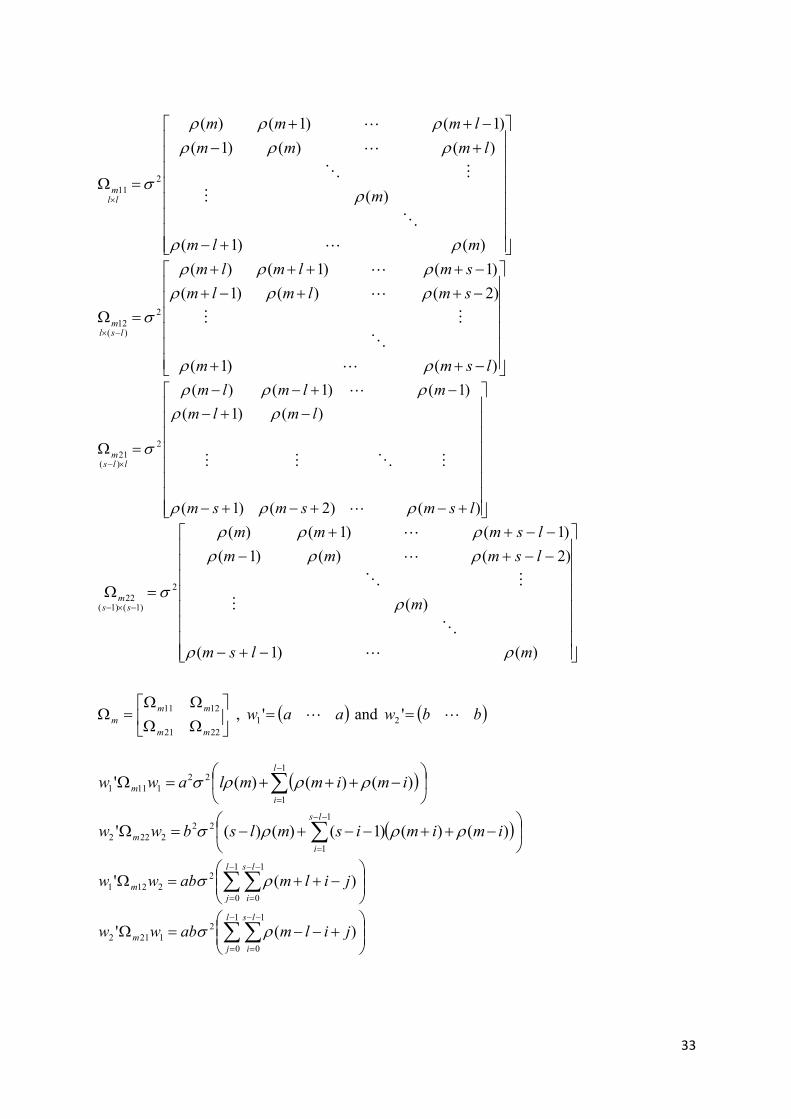
A6 Proof of Proposition 3
Decompose Ω into four pieces where 11Ω is ll× , 12Ω is )( lsl −× , 21Ω is lls ×− )( and
22Ω is )()( lsls −×− , also decompose ( )''' 21 www =
where '1w is s×1 and '1w is )(1 ls −×
Let
−=sl
a11
and
=s
b1
33
+−
+−
−++
=Ω×
)()1(
)(
)()()1(
)1()1()(
2
11
mlm
m
lmmm
lmmm
llm
ρρ
ρ
ρρρρρρ
σ
L
O
M
MO
L
L
−++
−++−+
−++++
=Ω−×
)()1(
)2()()1(
)1()1()(
2
)(12
lsmm
smlmlm
smlmlm
lslm
ρρ
ρρρρρρ
σ
L
O
MM
L
L
+−+−+−
−+−
−+−−
=Ω×−
)()2()1(
)()1(
)1()1()(
2
)(21
lsmsmsm
lmlm
mlmlm
llsm
ρρρ
ρρ
ρρρ
σ
L
MOMM
L
−+−
−−+−
−−++
=Ω−×−
)()1(
)(
)2()()1(
)1()1()(
2
)1()1(22
mlsm
m
lsmmm
lsmmm
ssm
ρρ
ρ
ρρρρρρ
σ
L
O
M
MO
L
L
ΩΩ
ΩΩ=Ω
2221
1211
mm
mm
m , ( )aaw L='1 and ( )bbw L='2
( )
−+++=Ω ∑
−
=
1
1
22
1111 )()()('l
i
m imimmlaww ρρρσ
( )
−++−−+−=Ω ∑
−−
=
1
1
22
2222 )()()1()()('ls
i
m imimismlsbww ρρρσ
−++=Ω ∑∑
−
=
−−
=
1
0
1
0
2
2121 )('l
j
ls
i
m jilmabww ρσ
+−−=Ω ∑∑
−
=
−−
=
1
0
1
0
2
1212 )('l
j
ls
i
m jilmabww ρσ

34
( )
( )
+−−+−+++
−++−−+−+
−+++
=
Ω+Ω+Ω+Ω=Ω
∑ ∑∑∑
∑
∑
−
=
−
=
−−
=
−−
=
−−
=
−
=
1
0
1
0
1
0
1
0
1
1
2
1
1
2
2
2222121221211111
)()(
)()()1()()(
)()()(
'''''
l
j
l
j
ls
i
ls
i
ls
i
l
i
mmmmm
jilmjilmab
imimismlsb
imimmla
wwwwwwwwww
ρρ
ρρρ
ρρρ
σ