TECHNICAL HANDBOOK

The installation of on-ground photovoltaic plants over marginal areas

PVs in BLOOM Project - A new challenge for land valorisation within a strategic eco-sustainable approach to local development

G. Nofuentes, J. V. Muñoz, D. L. Talavera, J. Aguilera and J. Terrados

2

INDEX 1. PV Grid-Connected Systems Basics

1.1. Overview 1.2. DC Part (PV modules, cabling, DC connection boxes, DC

switches) 1.3. AC Part (Inverter & energy meters) 1.4. Metal works and protective elements (earth electrode,

voltage surge arrestors, fuses, etc.) 1.5. Some electric characteristics of a typical 1-MWp PVPP BRIEF SUMMARY OF SECTION 1

2. Estimating The Annual Energy Produced by a PV Grid-Connected

System 2.1. Assessment on The Solar Resource of the Site (Available

insolation data sources: ground-based measurements and satellite-derived data)

2.2. Estimating The Annual Electricity Yield of a PV Grid-Connected System

BRIEF SUMMARY OF SECTION 2

3. Sizing PV Grid-Connected Systems

3.1. Choosing the PV module 3.2. Sizing the nominal power of the PV generator 3.3. Sizing the nominal power of the inverter 3.4. Sizing the number of modules 3.5. Sizing the number of series connected modules 3.6. Sizing the number of parallel connected 3.7. Sizing the cabling 3.8. Sizing protective measurements (fuses, voltage surge

arrestors, DC main switch, etc.)

3

3.9. Some characteristic data concerning implemented PVPPs BRIEF SUMMARY OF SECTION 3 APPENDIX OF SECTION 3: TERMINOLOGY

4. Matching PVPP Typologies to Specific Terrains

BRIEF SUMMARY OF SECTION 4

5. Economic Assessment on PV Grid-Connected Systems 5.1. Representative figures of the cost of PVGCS in some

countries 5.2. Existing supporting measures for PVPPs in each partner

country 5.3. Easy-to-use tables to estimate the IRR 5.4. Review of the most meaningful and understandable

profitability indices: the internal rate of return (IRR) 5.5. Easy-to-use tables to estimate the IRR 5.6. Short review of the taxation impact BRIEF SUMMARY OF SECTION 5

APPENDIX I OF SECTION 5. TABLES ADDRESSED TO ESTIMATE THE IRR

APPENDIX II OF SECTION 5: TERMINOLOGY

Appendix: Main technical and contractual points to be checked and compared when examining a proposal from an EPC supplier by a prospective owner

ACKNOWLEDGEMENTS

4

1. PV Grid-Connected Systems Basics

1.1 Overview

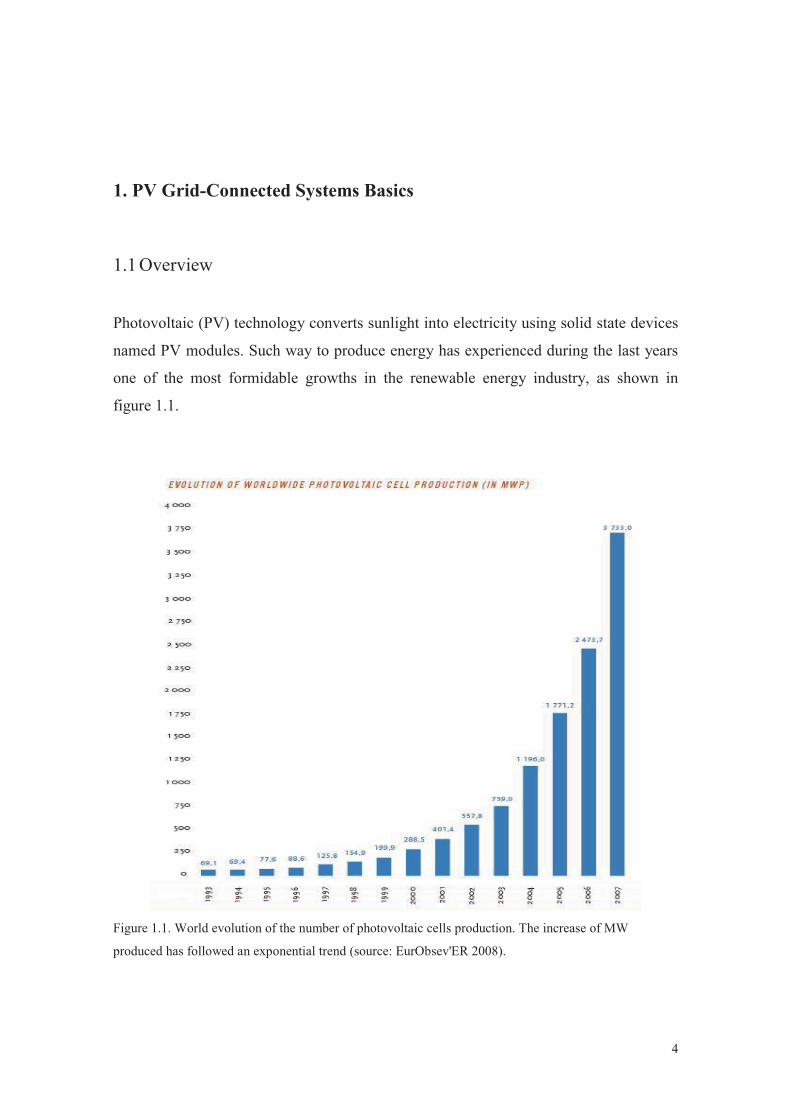
Photovoltaic (PV) technology converts sunlight into electricity using solid state devices

named PV modules. Such way to produce energy has experienced during the last years

one of the most formidable growths in the renewable energy industry, as shown in

figure 1.1.

Figure 1.1. World evolution of the number of photovoltaic cells production. The increase of MW

produced has followed an exponential trend (source: EurObsev'ER 2008).

5

PV systems may be grouped into stand-alone systems (SAPV) and grid-connected

systems (PVGCS). Basically the first one used the electricity produced to self-

comsuption while the second one the energy is sold through the electricity grid. Taking

into account the characteristics of the PV in Bloom project, the PV stand-alone systems

falls out of the scope of analysis of this paper, for this reason we are going to focus on

PVGCS. In this kind of PV systems all energy generated is fed into the company

electricity grid. In fact, the company plays the role of a huge energy store: in developed

countries, most PV systems are connected to the grid. In principle, this point makes

PVGCS simpler than SAPV mainly because it is not necessary to store any energy.

The reason of feeding all the energy PVGCS generates is related to the generous

existing feed-in tariffs, by which PV-generated electricity is sold to the grid at prices

well above the market. Further, the number of these systems has grown sharply

worldwide. This development has been brought mainly by means of a continuous

decrease trend in PV costs together with a wide variety of supporting policies that

diferent countries have launched (e.g.: Germany, Spain and Italy).

These strategies or policies are implemented with financial incentives, such as granting

a subsidy per kWp of installed capacity or a payment per kWh produced and sold -these

concepts will be explained in more depth in section 5 In other words, these financial

incentives broadly fall into generation-based (mainly implemented through generous

feed-in tariffs) and investment-focused (initial investment subsidies or rebates, low-

interest loans) ones. The latter incentives are being progressively phased out by

governmental bodies.

After this short approach to PVGCS a more in-depth study is to be accomplished

hereafter, dealing with the elements of these systems and how they work.

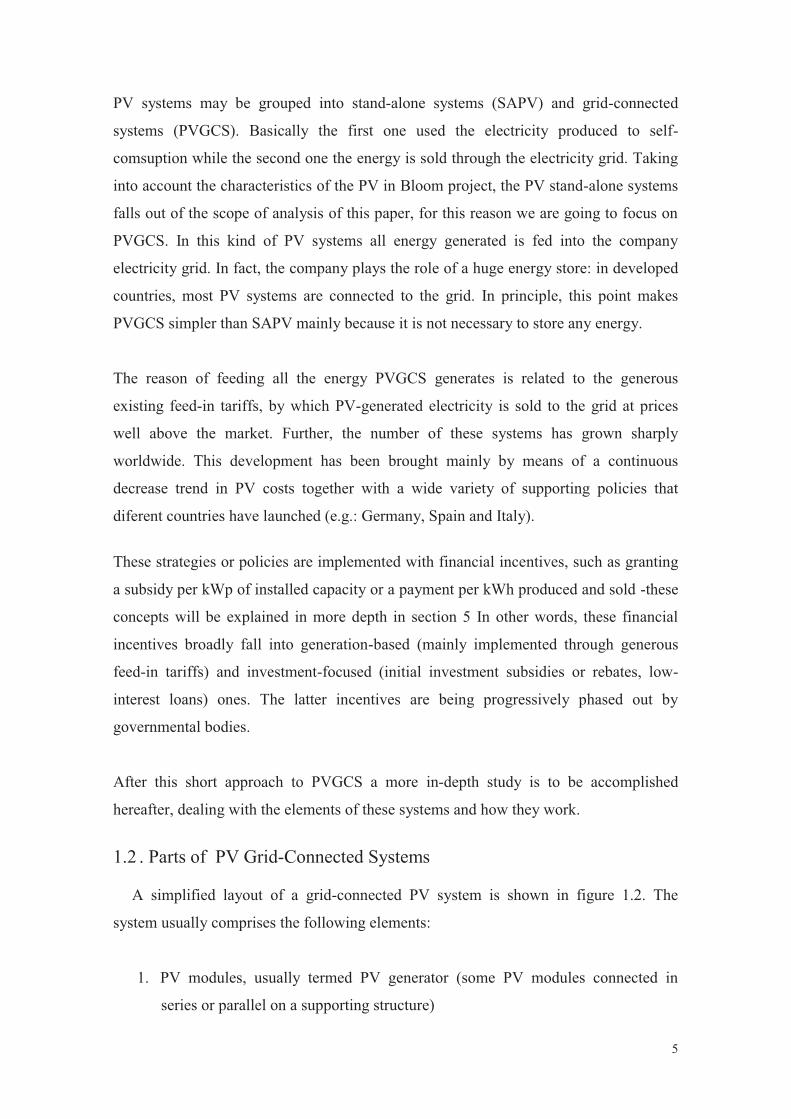
1.2 . Parts of PV Grid-Connected Systems A simplified layout of a grid-connected PV system is shown in figure 1.2. The

system usually comprises the following elements:

1. PV modules, usually termed PV generator (some PV modules connected in

series or parallel on a supporting structure)

6

2. Inverter (a solid-state based device that converts DC electricity from the

modules into AC electricity with the same characteristic as that supplied by the

grid)

3. Metering device intended to measure the electricity sold to the grid

4. Metering device intended to measure the electricity bought from the grid

5. AC loads from electrical appliances

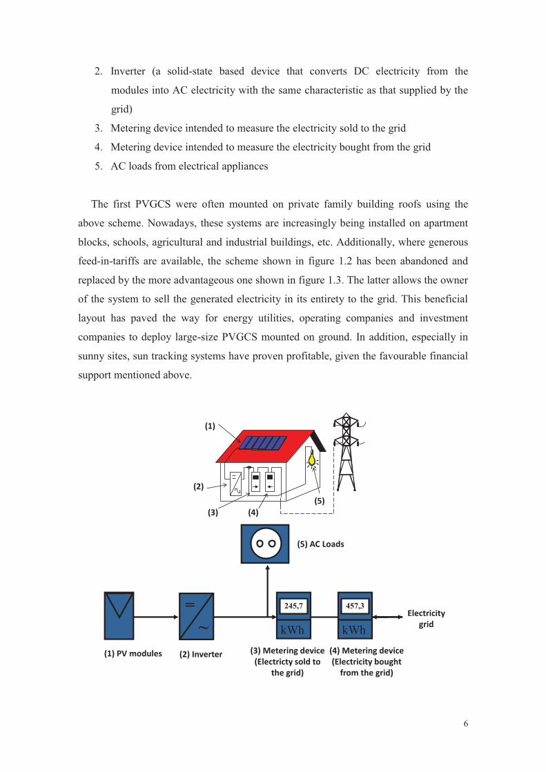
The first PVGCS were often mounted on private family building roofs using the

above scheme. Nowadays, these systems are increasingly being installed on apartment

blocks, schools, agricultural and industrial buildings, etc. Additionally, where generous

feed-in-tariffs are available, the scheme shown in figure 1.2 has been abandoned and

replaced by the more advantageous one shown in figure 1.3. The latter allows the owner

of the system to sell the generated electricity in its entirety to the grid. This beneficial

layout has paved the way for energy utilities, operating companies and investment

companies to deploy large-size PVGCS mounted on ground. In addition, especially in

sunny sites, sun tracking systems have proven profitable, given the favourable financial

support mentioned above.

(1) PV modules

=~

(2) Inverter

245,7

kWh(3) Metering device

(Electricty sold tothe grid)

(4) Metering device(Electricity bought

from the grid)

(5) AC Loads

Electricitygrid

457,3

kWh

(3)

(2)

(5)(4)

(1)

7

Figure 1.2. Simplified layout of a grid-connected PV system.

PV-generated electricity is partly sold to the grid

(1) PV modules

=~

(2) Inverter

245,7

kWh(3) Metering device

(Electricty sold tothe grid)

Electricitygrid

Figure 1.3. Simplified layout of a grid-connected PV system.

All the PV-generated electricity is sold to the grid

If the characteristics of electricity are taken into account, the diagram shown in figure

1.3 can be broadly divided in two parts.

DC PART: from the PV generator to the inverter input, the main characteristic in

this part is that the electricity is delivered as DC current. In this part PV modules,

supporting structures, wires and DC connection boxes are included.

AC PART: from inverter to public electricity grid, in this part the electricity is

delivered as AC current. In this part are included the following elements: inverter,

wires,protective elements and a metering device intended to measure the electricity

sold to the grid

.

8

This division is useful when a PVGCS and its constitutive elements are described.

Nevertheless there is a key element of grid connected systems which is related to the

DC and the AC parts; namely, metal works and earth electrode. Such elements are

elements of the safety system of PVGCS and are intended to protect against electrical

shocks.

1.2.1 DC Part

PV Modules, wires and connection boxes are the main elements that can be found in the

DC part. The DC character of current and operation of modules pose many questions

and new situations for novel electrical workers who are used to handling AC current.

1.2.1.1. PV Modules

PV modules are probably one of the most important elements of PVGCS, when the PV

modules are connected in serial and/or parallel configurations obtaining a PV generator.

At the same time, modules are made by connecting photovoltaic solar cells, which are

connected in series and parallel, to obtain higher current and voltage. To protect the

cells against mechanical stress, weathering and humidity, the cells are embedded in a

transparent material that also isolates the cells electrically. In most cases, glass is used

but depending on the process it is possible to use acrylic plastic, metal or plastic

sheeting. In contrast, the electrical connection of thin-film cells is an integral part of the

cell fabrication and is achieved by cutting grooves in the individual layers. Finally, the

standard modules have aluminium frame although it is possible to acquire frameless

modules.

Solar cells included in PV modules convert directly the solar radiation into electrical

energy. In the conversion process, the incident energy of the light creates mobile

charged particles in some materials, known like semiconductors, which are separated by

the device structure and produce electrical current. This current can be used to power an

electric circuit.

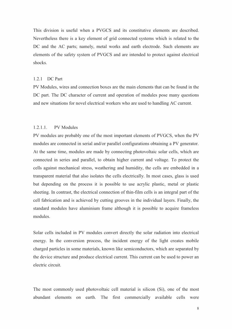
The most commonly used photovoltaic cell material is silicon (Si), one of the most

abundant elements on earth. The first commercially available cells were

9

monocrystalline silicon in which all the silicon atoms are perfectly aligned building an

organised crystal.In order to reduce costs, new manufacturing techniques were

developed which in turn gave birth to the polycrystalline solar cells. This type of

material contains many crystals and the atoms are aligned in diferent directions.

Figure 1.4. Main types of solar cells available in the present market

These techniques permit to manufacture solar cells in an easier, cheaper and faster way

using less pure silicon. In this sense, development of thin film technologies has

permitted further cost reductions by reducing the amount of material needed to make a

solar cell. Some materials other than silicon such as cadmium telluride (CdTe), copper

indium diselenide (CIS), amorphous silicon , etc. are used to manufacture solar cells.

Many diferent solar cells are now available on the market and yet more are under

development.

The types of modules are frequently divided according to the technology of the solar

cells incorporated. In this sense, it is common to find in literature monocrystal Si

modules, policrystal Si modules, amorphous Si modules, CdTe modules, CIS modules,

etc. Following this way, a more in-depth explanation of the most important solar cells

technologies existing nowadays is given below.

Crystalline silicon technologies.

10

The most important material for crystalline solar cells is silicon. This is the second most

abundant element on earth though it is never found as a pure chemical element. It is

bounded to oxygen in the form of silicon dioxide. So it is necessary to separate both

elements by means of a chemical process to get metallurgical silicon with a purity of

98%. This type of silicon cannot be used to produce solar cells due to its low purity. So,

it is necessary to apply another purification process which permits to obtain high-grade

silicon (at least 99:9999999% of purity). This high-grade silicon can now be processed

in diferent ways to produce monocrystalline or polycrystalline cells. It is not poisonous,

and it is environment friendly, since its waste does not represent any problem.

Among all kinds of solar cells the silicon solar cells are the most widely used. Their

efficiency is limited due to several factors. The energy of photons decreases at higher

wavelengths. The highest wavelength at which the photon energy is still large enough to

produce free electrons is 1.15µm (valid for silicon only). Radiation with higher

wavelength causes only heating up of solar cell and does not produce any electrical

current. Each photon can cause only production of one electron-hole pair. Even at lower

wavelengths many photonsdo not produce any electron-hole pairs, yet they increase

solar cell temperature. The highest achieved efficiency of a silicon solar cell in a

Research Lab lies around 23%, while for other semi-conductor materials this figure

rises up to 30%. In fact, eficiency is dependent on the semiconductor material. The

losses are caused by metal contacts on the upper side of a solar cell, in addition a part of

the solar radiation is reected on the upper side (glass) of solar cell. Crystalline solar cells

are usually wafers, about 0.3 mm thick, sawn from a Si ingot with a diameter of 10 to

15 cm. They generate approximately 35 mA of current per cm2 area (together up to 2

A/cell) at voltage of 550mV at full illumination. The effciency in Lab of the solar cells

exceeds 20%, while classically produced solar cells by commercial brands is usually

above 15%. Actually, there are potential types of silicon solar cells: monocrystalline

(single-crystalline), polycrystalline (both first types commented before) and amorphous.

Nevertheless to create the amorphous silicon cells it is necessary a special technique of

manufacturing, for this reason it is not usually catalog this cells together

monocrystalline or polycrystalline otherwise besides thin film.

Thin film cells

11

During the last years, the development of thin-film processes for manufacturing solar

cells has become more and more important. The process consists of applying a thin

layer of photoactive semiconductors on a substrate (usually glass). The most common

materials are: amorphous silicon (a-Si), thin multicrystalline silicon films on a low-cost

substract, copper indium diselenide (CIS) and cadmium telluride (CdTe).The reduced

material, the energy consumption and the automated production provides this

technology with a very high potential for reducing costs when compared with

crystalline silicon technology.

The amorphous silicon differs from crystalline silicon because silicon atoms are not

located at very precise distances from each other and this randomness in the atomic

structure has a powerful impact on the electronic properties of the material. The

manufacturing process consists in the deposition on a low-cost glass of diferent layers

of oxide, a-Si and a metallic contact. The efficiency of amorphous solar cells lies

typically between 6 and 8%. The lifetime of amorphous cells is shorter than the lifetime

of crystalline cells. Amorphous cells have current density of up to 15mA/cm2, and the

voltage of the cell without connected load of 0.8 V, a larger figure than that of

crystalline cells for this parameter. Their spectral response peaks at the wavelength

range of blue light: therefore, the ideal light source for amorphous solar cells is a

fluorescent lamp. The main disadvantage of the amorphous silicon is its low effciency

(6-8%) which even diminishes during the first 6-12 months of operation. After this

period of time, the efficiency gets a stable value. Related to the thin multicrystalline

silicon films, a conductive ceramic substrate containing silicon is covered with a thin

layer of polycrystalline silicon. The manufacturing process requires lower temperatures

so it is possible to obtain high quality semiconductors which have very high potential to

reduce costs.

Cadmium telluride (CdTe) is a thin-film material produced by deposition or by

sputtering is a promising low cost foundation for photovoltaic applications in the future.

The procedure disadvantage is that a poisonous material (cadmium) is used in its

manufacturing, although some manufacturers support an insurance policy approach to

funding the estimate futurecosts of reclaiming and recycling their modules at the end of

their use. Labsolar cells efficiency is up to 16%, whilst the commercial types efficiency

is up to 8%.

12

Copper-indium-diselenide (CuInSe2, or CIS) is a thin-film material with efficiencies

ranging from some 13% in marketed modules to some 17% achieved at Research Labs.

This is a is promising material, yet not widely used due to production specific

procedures and to the scarcity of indium. Table 1.1 summarises the main characteristics

of commercial solar cells.

Table 1.1. Main characteristics of commercial solar cells

Material Efficiency Nominal power degradation after

22-year outdoor exposurea

Colour

Monocrystal

Si

15-22% 14,8% (TedlarTM and EVA

encapsulant)

Dark blue

Multicrystal

Si

13-15% 6,4% (Transparent silicon

encapsulant)

Blue

Amorphous Si 8-15% N/A Red-blue, black

CdTe 6-9% N/A Dark green, black

CIS 7.5-9.5 N/A Black a Source: Ewan D. Dunlop and David Halton, The Performance of Crystalline Silicon Photovoltaic Solar Modules after 22 Years of Continuous Outdoor Exposure, Prog. Photovolt: Res. Appl., DOI: 10.1002/pip.627

Nowadays, the PV market offers a huge range of the power output of the PV modules. It

is possible to acquire PV modules from a few watts to several hundred of watts and the

number of the companies which offer PV modules in the world is very high. A typical

standard module consists of 36-72 cells and the power ranges from 75-270 Wp, in the

case of crystalline cells. Sometimes, in some operation conditions solar cells in a PV

module can be shaded and their temperature may increase until it causes damage in the

material. This situation is known like ‘hot spots’ and when it appears the nominal power

delivered by module is reduced dramatically. In order to avoid and prevent hot spots,

the PV modules must incorporate bypass diodes. Usually, a bypass diode is connected

to protect 18-20 solar cells.

1.2.1.2. Cabling

The cabling of a PV installation is addressed to carry the electricity from the PV

generator to the inverter and from the inverter to grid electricity company. It means that

13

the cabling is required in both DC and AC parts. Special attention must be paid in DC

cabling because the features of DC current make this part more dangerous than AC if a

shortcircuit takes place. For this reason it is advisable to use a isolation level category II

in all wires used, so these types of cables have a double coating to make the cabling

more resistant to weather conditions. In addition, the current that flows in the DC part

(in most cases higher than that which ows in the AC part) makes advisable to use a

suitable cable section to avoid losses in electrical production. In this sense, it has to be

followed the advise which claims that the voltage drop in the cabling must not exceed

1.5%. Section 3 will resume this issue in order to size the suitable cross-section of the

cabling in a PV installation.

Last, in order to make a correct layout of the cabling, it is advisable that the positive

pole and negative pole are separated and clearly differentiated. In this sense the colour

of the positive cable pole must be different than that of the negative, using in the most

of the cases warm colours for the positive (i.e. red) pole and cold colours for negative

pole (i.e. black). In the AC part it is advisable to use differentiated colours between

phases and neutral-ground too.

1.2.1.3. Connection boxes

Connection boxes are the elements where the strings of the PV generator are connected.

The connection boxes role is two-fold: first, it ensures a weatherproof connection

between strings and second, it includes several safety devices very advisable to protect

the installation against electrical failures and weather problems like short circuits by

humidity or degradation by prolonged exposure to solar UV radiation. Figure 1.6 will be

used to illustrate and explain the elements included in DC connection boxes.

1. Each string from the PV generator must be guided to the connection box

separately, positives lines bundled on one side and negatives ones bundled to

another. This measure ensures a safety physical distance between positive and

negative poles avoiding short circuits and enabling easy maintenance works.

2. Each string has a fuse to protect the line against reverse currents. The reverse

currents may appear when one of the strings has a failure and the current of

another strings flow through this faulty string.

14

3. Voltage surge arrestors (varistors) arrest possible overvoltages (e.g.: induced

voltages in cable loops owing to lightning strikes near the installation) that may

appear in the PV generator.

4. The DC switch is a very advisable element in order to break the flow of the DC

current from generator to inverter.

Figure 1.6. State-of-the-art DC connection box. All its elements have a good placement and are accessible

(Courtesy of Suntechnics)

5. All metal works and outputs from varistors must be connected to earth electrode.

6. The output cabling must be guided to the inverter or to another connection box.

Obviously, the cross-section of these output wires must be higher that string

cables.

15

1.2.2 AC Part

The inverter(s), AC cabling, the DC main switch (and both the magnetothermic switch

and the residential current circuit breaker) together with the energy meters are the main

elements that are to be found in the AC part. The inverter is the paramount element in

this part as the energy meter is a device chosen and installed by the electricity company

in most of the cases. In fact, the inverter converts DC current into AC current of the

same characteristics as those of the grid. This is way the inverter(s) are crucial elements

in PV plants.

1.2.2.1. Inverter

Grid-connected inverters are also known as grid-tied inverters. This device (figures 1.2

and 1.3) connects the PV array to the grid, or to both the grid and the AC loads of a

building. It is mainly devoted to convert the solar DC electricity into AC electricity of

the same characteristics as those of the grid, as commented above. The performance of

these devices has significantly improved during the recent past and only small losses

take place in this conversion. In PVPPs, as a particular case of PVGCS, the inverter is

connected directly to the grid following the scheme depicted in figure 1.3, so all the

generated electricity is fed into the grid.

16

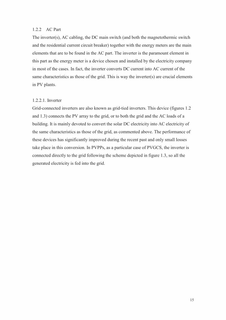
Figure 1.7. Image of a 100-kW power rated inverter

during the realization of a quality check.

PVGCS using inverters up to a power of 5 kW usually are usually single-phase systems.

When this figure is exceeded, three-phase inverters are used (Figure 1.7). Making the

most of the voltage-current curve of the PV generator requires the inverter to operate in

the maximum power point (MPP) of this curve. This point ceaselessly changes

according to environmental conditions, so suitable electronic devices must be available

inside the inverter to track this MPP and maximize the DC power input.

Inverters often incorporate built-in trans-formers to electrically isolate the PVGCS from

the grid. Transformerless inverters are smaller and lighter but not all national electrical

regulation codes addressed to grid connected PV allow the use of such devices (i.e: the

Spanish regulations do not allow to use transformerless inverters, while German

regulations do).

17

The conversion efficiency (η) is the parameter is the ratio between the output AC power

and the input DC power. This parameter takes into account losses caused by the

transformer –if this device is built into the inverter- ohmic elements, switching devices,

etc. It is worth noting that conversion efficiency depends on the input DC power: this is

especially noticeable at low levels of irradiance impinging on the PV generator, which

causes a lower load to be connected to the inverter. Manufacturers usually provide a

curve depicting conversion efficiency versus output AC power: state-of-the-art inverters

may achieve a peak in this curve of some 95%. In order to make sound efficiency-based

comparisons of inverters, a reasonable way of measuring efficiency taking into account

different climate conditions (Euro efficiency, or η Euro) was introduced by defining the

Euro efficiency (η Euro).

The Euro efficiency is a parameter weighted for the European climate, taking into

account different load conditions due to climate. Parameter η Euro is stated as:

0.2 0.48 0.1 0.13 0.06 0.03 100%50%30%20%10%5%Euro 10503020105%E 000000 (1.1)

Where the subscript of parameter η refers to the efficiency of the inverter at a load

expressed as a percentage of the nominal AC load (100%) which corresponds to η 100% .

It must be pointed out that the different weights assigned to each figure of η at different

loads was carried out bearing in mind the Central European climate. State-of-the-art

inverters may achieve a η Euro ranging from 92 to 96 per cent.

1.2.2.2. Energy meters

The energy meter (figure 1.8) is the element aimed at measuring the AC electricity

produced by the PV installation. This device is placed just before the connection point

of the grid, after the inverter. Obviously, the energy meter is a device installed and

checked by the grid electricity company so that neither the installer or the owner of the

PV system may manipulate it, for obvious reasons.

18

Figure 1.8. Three-phase energy meter with a monitoring and communication system.

Almost all the energy meters installed nowadays have a monitoring system to store the

readings. Then, the readings are accessible for both the installation owner and the

electricity company.

1.2.3 Metal works and earth electrode

Both AC and AC parts have conductive metal works which may be accessible to people.

The earth electrode is a protective element meant to prevent these metal works from

rendering electrical shocks to persons. In fact, a dangerous situation may take place if a

DC or AC wire experiences an isolation fault and it gets in touch with a metal part of

the installation. In this sense and to prevent risky situations like this one, all the metal

works of the PV installation such as the inverter chassis, module frames, DC connection

boxes must be connected with the earth electrode. In this case, if an isolation fault

appears, the earth electrode would play the role of a drain that avoids the risk of an

electrical shock. In addition, one of the terminals of the surge arresters is connected to

19

the earth electrode: this element provides the way to drain the overcurrent that is carried

through these surge arresters.

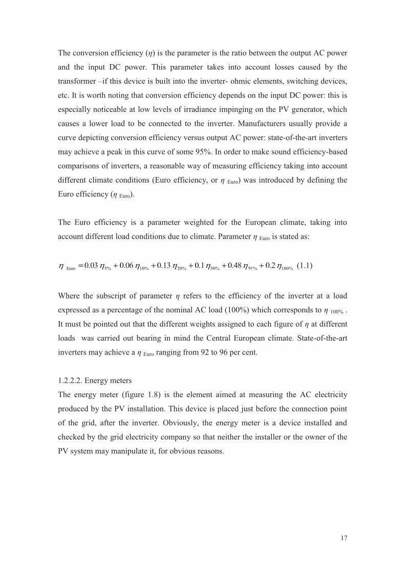
In spite of being not an active part of the PVGCS, the earth electrode connected to the

metal works are the key to solve safety problems related to isolation failures,

overcurrents and overvoltages. Since the PV plants are usually ungrounded for the sake

of safety –and many national electrical regulation codes enforce this electrical scheme-

none of its poles (positive o negative) are connected to the earth electrode, the correct

design of this element is an issue to be attended carefully. Thus, it is highly advisable

that the resistance of earth electrode do not be over to 37 ohms. In addition, the

connection between all the metal works and the earth electrode must be easily visible

and accessible in order to check the system safety (figure 1.8).

Figure 1.8. Connection point between the earth electrode and various metal works in a PV installation.

20

1.5. Some electrical characteristics of a typical 1-MWp PVPP Given the wide variety of existing marketed devices used to build PVPP’s within the

power range that the ‘PVs in Bloom’ project is focused on (50 kWp - 2 MWp) and the

different technical solutions that may be adopted to install a PVPP of a given peak

power, it is difficult to furnish the reader with some typical electrical characteristics of

such systems. However, an example of a typical PVPP of some 1-MWp implementation

may help get an idea of the range of voltage, current and power these systems deal with.

A widespread technical solution aimed at deploying large-scale PVPPs (with rated

power equal or greater than 1-MWp) may consist of dividing it into smaller PV

subsystems. A state-of-the-art feasible solution may comprise ten 120-MWp

subsystems. Each subsystem PV generator is connected to a 3-phase 100-kW inverter

whilst each couple of inverters are fed to a 400-kVA 380V / 20 kV1 transformer (five of

such transformers are required in total). Figure 1.9 depicts the electric scheme for such a

1.2-MWp PVPP. In this figures, the ten energy meters (one for each inverter) may also

be replaced for just only one placed at the high voltage output of the transformer. In

fact, placing the energy meter at either the low voltage input or the high voltage output

of the latter device usually has to do more with legal matters than with technical

constraints

1 The figure for the high voltage side of the transformer may vary depending on the country electrical distribution system. The nominal power of the transformer is deliberately oversized up to twice the inverter connected power.

21

=~

245,7

kWh

=~

345,2

kWh

Two 120-kWp PVgenerators

Two 100-kW 3-phase inverters

400-kVA 380 / 20 kVtransformer

5 X GRI

D

Figure 1.9. Electric scheme of a possible technical solution for a 1.2-MWp PVPP.

The main electrical characteristics in STC of the PV generator of each one of these

possible ten subsystems are gathered in Table 1.2.

Table 1.2. Main electrical characteristics in STC of the PV generator of a subsystem of the typical PVPP

of some 1 MWp described in this section. The figures for these electric characteristics have been chosen

taking into account state-of the art crystalline silicon modules and inverters –which drive the selection of

series-connected and parallel-connected modules- marketed at the date of writing this document

Nominal power

(Wp)

Open-circuit

voltage (V)

Short-circuit

current (A)

Voltage at

maximum power

point (V)

Current at

maximum power

point (A)

120 000 790 205 631 190

BRIEF SUMMARY OF SECTION 1

Throughout section 1 the main features of a photovoltaic grid connected system

have been detailed. In order to describe these systems, a suitable division has

been done. In this sense, any of these systems is roughly compounded of three

22

different parts. So, each part is commented and its constitutive elements have

been approached

DC part: it stretches from the PV generator to the inverter input; the main

characteristic in this part is that the electricity is delivered as DC current. PV

modules, supporting structures, protective elements, wires and DC connection

boxes are included in the DC part. The characteristics (efficiency, encapsulation,

degradation, etc.) and types (monocrystal, policrystal or thin film) of PV cells

and PV modules have been emphasized in this section.

AC part: it stretches from the inverter to public electricity grid; in this part the

electricity is delivered as AC current. Inverter, wires, protective elements and a

metering device intended to measure the electricity sold to the grid. The inverter

efficiency has been emphasized in this section, including equations to calculate

this parameter.

Metal works and earth electrode: this part is aimed to avoiding electrical shocks

to people. Concepts like overcurrents and overvoltages in PV plants together

with the elements addressed to prevent these failures have been presented

Some electrical characteristics of a typical 1-MWp PVPP are provided to help

the reader to achieve a better understanding of this PV concept

23

2. Estimating the annual energy produced by a PV grid-connected

system

Although the cost of a typical on-ground PV installation ranging from 50 kWp to 2

MWp (the size range of the PVPPs that the project PVs in Bloom deals with) has

dramatically been reduced by some 35% during the years 2007-2009, the initial

investment the installation requires forces the prospective owner in many cases to take

money on loan from a bank. The future energy production of the plant is the best

warranty for the owner –and for the bank, of course- in order to acomplish the payment

of the loan. This fact may help to get an idea of the importance of making a good

estimate of the annual energy produced by a PV grid-connected system. This section

aims at explaining how to calculate the annual electricity yield of a PV grid-connected

system. In addition, the online existing tools to evaluate the solar resource (the main

uncertainty source) are going to be detailed hereafter as well.

2.1 Assessment on the solar resource of the site Knowing the solar resource is the first step to evaluate the annual production of a PV

plant. This means that it is necessary to know the annual incident irradiation on the PV

generator. In addition, both the module slope (β, or tilt angle, which lies between 0º and

90º) and orientation (α, or azimuth, East = -90º, South = 0º, West = 90º) have to be

taken into account in this issue because the irradiation received over one year by a

surface with an arbitrary tilt angle and azimuth may largely differ from the irradiation

collected by a horizontal surface (the most common available irradiation data in solar

databases). There are some methods to determine the former parameter from the latter,

but they lie out of the scope of this work. Anyway, it is useful to know that an Equator-

facing PV generator –it implies South-facing (α = 0º) and North-facing (α = 180º) for

North and South hemispheres, respectively- with a tilt angle slightly lower than the

local latitude (βopt) maximizes the collected annual global irradiation and consequently

maximizes the electricity generation. Figure 2.1 illustrates the features related to the tilt

angle β and the azimuth α.

24

Figure 2.1.: Slope and orientation of a PV generator (source: IDAE, 2002. Instalaciones de Energía Solar Fotovoltaica. Pliego de Condiciones Técnicas de Instalaciones Conectadas a Red. IDAE, Madrid, p.53)

Before starting to introduce how to evaluate the solar resource, it is interesting to

explain what the irradiation is and what the differences between irradiation (H) and

irradiance (G) are. In order to see the difference between these two terms, Figure 2.2

may be useful for this purpose. Figure 2.2-A depicts a graph of measured irradiance vs.

time during a sunny day. As it is shown, the irradiance has units of watts per square

meter (W/m2) so the irradiance is the incident sunlight power density. Since the

irradiance is nothing but sunlight power per square meter, the instantaneous character of

the irradiance has to be emphasized. In Figure 2.2-B, the area under the latter irradiance

curve and x-axis has been coloured in red: this area is the irradiation collected over this

day. Thus, the irradiation has units of W•s/ m2 or kWh/m2: this means energy collected

per square meter during a specific time interval. If the considered time interval is a day

or a year, the terms ‘daily irradiation’ or annual irradiation’ may be used.

Figure 2.2. Graph A depicts the measured irradiance during a sunny day whilst the red area of graph B

equals the collected irradiation during this sunny day

25

Given the statistical nature of the irradiation profile of a site, annual or monthly average

values for the daily irradiation (Hda(0) and Hma(0), respectively) are commonly used

when designing PV systems. As commented earlier, these average values are available

only for horizontal surfaces in most solar databases. However, for installations located

in European sunny climates and with an optimun tilt angle, equation 2.1 is a rule-of-

thumb that broadly relates the annual average horizontal irradiation -H(0)- and the

annual average irradiation collected on a equator-facing, βopt –tilted surface -H(0,βopt):

]year·m·kWh)[(H.]year·m·kWh)[,(H opt

1212 01510 1212 1op (2.1) This obviously means that:

36501513650 1212 ]·day·m·kWh)[(H.]·day·m·kWh)[,(H daoptda

1212 1op (2.2) This is:

]day·m·kWh)[(H.]day·m·kWh)[,(H daoptda1212 01510 1212 1op (2.3)

If irradiation collected on surfaces with an arbitrarily azimuth angle α and tilt angle β is

to be estimated -H(α,β)- some graphs proposed in literature may be of great help. Thus,

figure 2.3 is intended to derive the latter value from H(0) and it can be applied to similar

range of latitudes to those of Spain (i.e.: Southern European countries). An example is

provided to achieve a better understanding of its use.

26

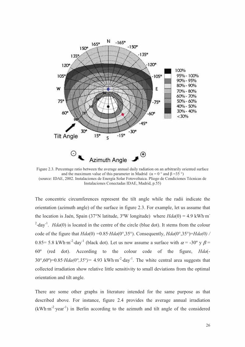
Figure 2.3. Percentage ratio between the average annual daily radiation on an arbitrarily oriented surface

and the maximum value of this parameter in Madrid (α = 0 ° and β =35 °) (source: IDAE, 2002. Instalaciones de Energía Solar Fotovoltaica. Pliego de Condiciones Técnicas de

Instalaciones Conectadas IDAE, Madrid, p.55) The concentric circumferences represent the tilt angle while the radii indicate the

orientation (azimuth angle) of the surface in figure 2.3. For example, let us assume that

the location is Jaén, Spain (37°N latitude, 3ºW longitude) where Hda(0) = 4.9 kWh·m-

2 day-1. Hda(0) is located in the centre of the circle (blue dot). It stems from the colour

code of the figure that Hda(0) =0.85·Hda(0°,35°). Consequently, Hda(0°,35°)=Hda(0) /

0.85= 5.8 kWh·m-2 day-1 (black dot). Let us now assume a surface with = -30º y =

60º (red dot). According to the colour code of the figure, Hda(-

30°,60º)=0.85·Hda(0°,35°)= 4.93 kWh·m-2 day-1. The white central area suggests that

collected irradiation show relative little sensitivity to small deviations from the optimal

orientation and tilt angle.

There are some other graphs in literature intended for the same purpose as that

described above. For instance, figure 2.4 provides the average annual irradiation

(kWh·m-2·year-1) in Berlin according to the azimuth and tilt angle of the considered

27

surface. The relative shape of the contour lines –not the specific values of the average

annual irradiation- may apply to Central European climates

Figure2.4. Average annual irradiation (kWh·m-2·year-1) in Berlin depending on the azimuth and tilt angle

(Source: DGS and Ecofys, 2005. Planning and Installing Photovoltaic Systems. A guide for installers, architects and engineers, James & James, London, p. 13)

Two-axis tracking in Southern Europe may achieve irradiation gains up to some 40% when

compared to static surfaces optimally oriented and tilted (0,βopt). This gain lowers down to some

30% in Central Europe, due to its cloudier climate. Single-axis tracking in Southern Europe may

achieve irradiation gains up to some 25-33% -depending on the tracking method- when

compared to static systems to static surfaces optimally oriented and tilted (0,βopt). This gain

lowers down to some 20% in Central Europe, owing to the same fact as that mentioned earlier.

Apart from the above graphical methods, there are some convenient software tools

addressed to evaluate the irradiation on an arbitrarily inclined and oriented surface for a

specific site (determined by its latitude and longitude). Most of this software tools work

with a data base obtained through two ways: data collected by ground-based

measurements and/or satellite-derived data. These software applications usually have a

software engine which is able to evaluate the irradiation through complex interpolation

methods taking into account the data from several meteorological stations and/or

satellite observations around the placement of the PV plant.

In this sense, programs like Meteonorm, Sundy and Shell Solar Path make possible and

easy to evaluate the annual irradiation of a given site. There are some free online

software tools to estimate the irradiation too. In this way, for Europe and Africa

locations, the EC-funded PVGIS project (http://re.jrc.ec.europa.eu/pvgis/) gives support

28

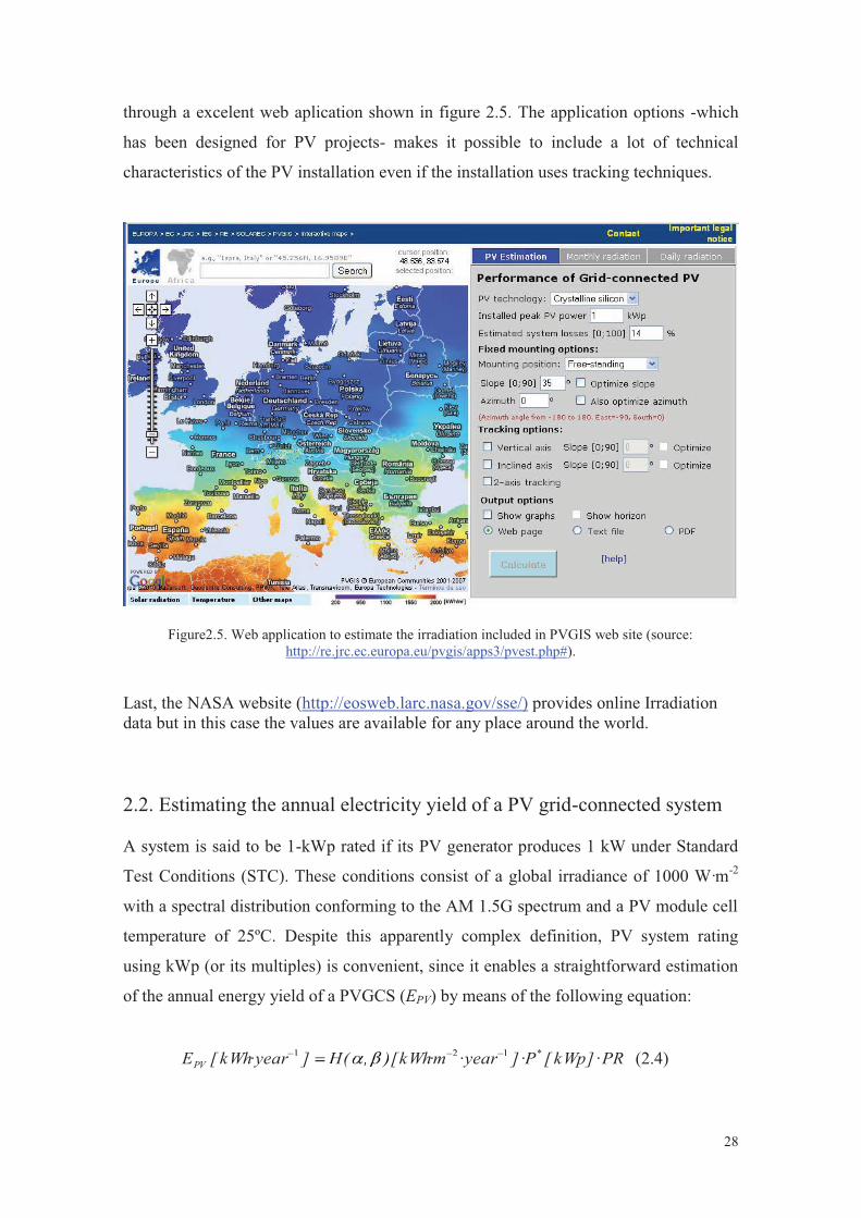
through a excelent web aplication shown in figure 2.5. The application options -which

has been designed for PV projects- makes it possible to include a lot of technical

characteristics of the PV installation even if the installation uses tracking techniques.

Figure2.5. Web application to estimate the irradiation included in PVGIS web site (source: http://re.jrc.ec.europa.eu/pvgis/apps3/pvest.php#).

Last, the NASA website (http://eosweb.larc.nasa.gov/sse/) provides online Irradiation data but in this case the values are available for any place around the world. 2.2. Estimating the annual electricity yield of a PV grid-connected system A system is said to be 1-kWp rated if its PV generator produces 1 kW under Standard

Test Conditions (STC). These conditions consist of a global irradiance of 1000 W·m-2

with a spectral distribution conforming to the AM 1.5G spectrum and a PV module cell

temperature of 25ºC. Despite this apparently complex definition, PV system rating

using kWp (or its multiples) is convenient, since it enables a straightforward estimation

of the annual energy yield of a PVGCS (EPV) by means of the following equation:

PR·]kWp[P·]year·m·kWh)[,(H]year·kWh[E *PV

121 r 12r 1 H ),( (2.4)

29

Where P* = PV generator power in STC and PR = performance ratio

The performance ratio is related to the efficiency of the system together with many

other losses that inevitably take place –operation temperature losses, power

conditioning and wiring losses, etc- and influence electricity generation in PV systems.

PR values for well designed PVGCS may be assumed ranging from 0.70 to 0.80. These

figures are in good agreement with many available performance data.

An example may help to achieve a better understanding of eqn. (2.4). Let us assume a 1-

MWp PVGCS located on a site where the average annual irradiation on the PV

generator equals 1900 kWh·m-2·year-1. If a figure of 0.7 is assumed for the performance

ratio of the system, then:

1121 ·13300007.0·1000···1900)·( 1121 11 yearkWhkWpyearmkWhyearkWhEPV

A commonly used parameter to assess the amount of solar electricity produced by a

PVGCS is the final yield (Yf, in kWh·kWp-1·year-1). Figure 2.6 depicts some minimum

and maximum values for this parameter in some countries. Also, Table 2.1 gathers some

typical values for this parameter calculated in some specific sites located in each project

partner country.

30

Figure 2.6. Minimum and maximum annual PV electricity yields in different countries produced by a 1-

kWp system (kWh year-1) with optimally inclined PV modules and performance ratio equal to 0.75. (Sources: European Commission Joint Research Centre,

http://re.jrc.cec.eu.int/pvgis/apps/pvest.php?lang=en&map=Europe; and National Renewable Energy Laboratory, http://www.nrel.gov/rredc/pvwatts/).

Table 2.1 Typical values for this parameter calculated in some specific sites located in each project

partner country. N.B.: PVGIS software has been used. Equator-facing and optimally tilted static

structures together with a performance ratio that equals 0.8 have been assumed

Place Latitude, longitude Optimal tilt angle (º) Yf, (kWh·kWp-1·year-1)

Representative places from Italy

Padova (Italy) 45.410N, 11.877E 34° 1144

Belluno (Italy) 46.140N, 12.218E 36º 1096

Berchidda (Italy) 40.785N, 9.166E 34° 1456

Lugo di Vicenza (Italy) 45.746N, 11.530E 35º 1112

Mores (Italy) 41.474N, 1.564E 34º 1376

Sassari (Italy) 40.727N, 8.56E 34° 1456

Siliqua (Italy) 39.301N, 8.81E 34° 1472

Representative places from Greece

Afetes (Greece) 39.283N, 23.18E 30° 1328

Aiginio (Greece) 40.511N, 22.54E 31° 1280

Lefkonas (Greece) 41.099N, 23.50E 31° 1224

Milies (Greece) 39.328N, 23.15E 30° 1352

Sourpi (Greece) 39.103N, 22.90E 29° 1304

31

Representative places from Poland

Adamow (Poland) 50.595N, 23.15E 35° 936

Gmina Wisznice (Poland) 51.789N, 23.21E 36° 944

Urzad Miasta Lublin (Poland)

51.248N, 22.57E 36° 936

Representative places from Austria

Burgau (Austria) 48.432N, 10.41E 36° 1000

Fürstenfeld (Austria) 47.095N, 15.98E 35° 1064

Representative places from Slovakia

Drahovce 48.518N, 17.80E 35° 1040

Bacuch 48.859N, 19,81E 38° 1024

Representative places from Spain

Valencia 39.470N, -0.377E 35° 1400

Jaén 37.766N, -3.790E 33° 1544

Alcaudete 37.591, -4.087E 33° 1560

Hornos 38.217N, -2.720E 32° 1520

BRIEF SUMMARY OF SECTION 2

Explaining how to calculate the solar irradiaton collected on a surface with a

given orientation (α) and tilt angle (β), paves the way to calculate the energy

produced by a PV plant.

Some graphical methods have been provided to estimate the solar irradiaton

collected on an arbitrarily oriented and tilted surface. (H(α ,β)). Some software

tools addressed to the same purpose have been introduced

An equation that combines accuracy and simplicity aimed at calculating the

annual energy production of the installation has been presented:

PR·]kWp[P·]year·m·kWh)[,(H]year·kWh[E *PV

121 r 12r 1 H ),(

Where P* = PV generator power in STC and PR = performance ratio (0.7-0.8)

32

3. Sizing PV grid-connected systems This section deals with the basic concepts aimed at sizing a PV grid-connected system

deployed on a degraded area (a PVPP). Accomplishing an in-depth explanation of how

to design a PVPP by means of a rigorous and universal approach, covering each

configuration, would encompass nearly every possible case. On the other hand, this

would require much more effort and would reduce the understandability of the text.

Consequently, the concepts presented hereafter have been simplified to some extent and

only sizing flat-plate module PVGCS with central inverter is studied.

3.1. Choosing the PV module

The used PV modules highly determine the sizing of the remaining PVGCS elements. A

rough estimate of 10 m2 of required area per installed kWp is useful as a first approach.

Taking into account the present state of the art, more accurate estimations are gathered in

table 3.1, depending on the solar cell technology. Mono and polycrystalline silicon solar

cells still hold the lion’s share of the PV market, but new promising technologies like that

based on CdTe are increasing their presence in it.

1 kWp 10 m2 of required surface (crystalline silicon) if the PV modules are deployed in

the same plane as the surface –roof or terrain- on which they are supported

It is worth noting that the above considerations are true if the PV modules are deployed in

the same plane as the surface –roof or terrain- on which they are supported. This is not the

case in most PVPPs. In PVPPs, making an estimate of the required area for the system

may turn into a complex problem which involves local latitude, terrain slope, module tilt

angle, etc. However, for the sake of simplicity, the following statements will be assumed:

horizontal terrain surface, tilt angle slightly lower than the latitude, and no self shadowing

between PV module arrays. Taking into account the present state of the art as above, table

3.2 shows the required terrain surface to install a 1-kWp PVGCS, depending on the solar

cell technology.

Table 3.1. Required surface for a 1-kWp PVGCS if PV modules are deployed in the same plane as the

surface –roof or terrain- on which they are supported (Source: DGS y Ecofys, 2008. Planning and Installing

33

Photovoltaic Systems. A guide for installers, architects and engineers. Second Edition. James & James,

London, p. 151)

Technology Surface (m2)

Monocrystalline silicon 7-9

Polycrystalline silicon 8-11

Copper Indium Diselenide (CIS) 11-13

Cadmium Telluride (CdTe) 14-18

Amorphous silicon 16-20

1 kWp 20 m2 of required surface (crystalline silicon) if the PV modules are deployed

on an horizontal terrain surface, tilt angle slightly lower than the latitude and with no self-

shadowing between PV module arrays

Tabla 3.2 Required surface for 1-kWp if the PV modules are deployed on an horizontal terrain surface, tilt

angle slightly lower than the latitude and with no self-shadowing between PV module arrays. Note: the

figures gathered here are somewhat overestimated. More accurate calculations for each specific latitude may

lead to smaller values of the required surface

Technology Surface (m2)

Monocrystalline silicon 20

Polycrystalline silicon 27

Copper Indium Diselenide (CIS) 32

Cadmium Telluride (CdTe) 40

Both inverter and PV modules manufacturers supply the most characteristic electrical

parameters of their products. The most relevant ones are shown in Tables 3.3 and 3.4. As it

will be shown hereafter, these parameters are paramount for the system design. Some other

features such as weight, dimensions, etc. are also usually enclosed in the manufacturer data

sheets

34

Table 3.3. Most relevant electrical parameters of a PV module usually supplied by its manufacturer

Parameter Symbol Short circuit current temperature coefficient (mA·ºC-1) IMOD,SC Open circuit voltage temperature coefficient (mV·ºC-1) VMOD,OC Current at the MPP at STC (A) IMOD,M,STC Short circuit current at STC (A) IMOD,SC,STC Parallel connected cells Ncp Series connected cells Ncs Maximum power at STC (Wp) PMOD,M,STC Nominal operation cell temperature (ºC) NOTC Voltage at the MPP at STC (V) VMOD,M,STC Open circuit voltage at STC (V) VMOD,OC,STC

Table 3.4. Most relevant electrical parameters of an inverter usually supplied by its manufacturer

3.2. Sizing the nominal power of the PV generator Planning the nominal power of a PV generator (the sum of the maximum power at STC

of the modules used) may depend on two criteria. It is up to the owner to select the most

restrictive one:

- Available area: this is especially crucial, and table 3.2 must be kept in mind

Parameter Symbol

Maximum efficiency (adim) INV,M

Power factor (adim) cos

Grid frequency (Hz) f

Maximum input DC current (A) IINV,M,DC

Nominal output AC current (A) IINV,AC

Lowest voltage at which the inverter tracks the MPP (V) VINV,m,MPP

Highest voltage at which the inverter tracks the MPP (V) VINV,M,MPP

Nominal input power (W) PINV,DC

Nominal output power (W) PINV,AC

Maximum input voltage (V) VINV,M

Nominal output voltage (V) VINV,AC

35

- Cost of the installed PVGCS. Nowadays, a rough estimate of the initial

investment on the system may range from some 3,000 to 6,000 Euro. Anyway,

the cost of crystalline silicon modules has experienced a sharp decline during the

years 2007-09 and it seems this downward trend will continue in the short-term.

The PV generator is composed by arranging parallel connections between series-

connected modules (strings). Consequently, the voltage of the PV generator equals the

voltage of one string, whilst its current equals the sum of the current of all parallel

connected strings.

3.3. Sizing the nominal power of the inverter

Prior to provide some guidance aimed at sizing the nominal power of the inverter, some

advice must be provided regarding its location. In general, the inverter must be close to

the AC protective devices (surge arresters, residual current circuit breaker, etc.) and the

energy meter. It is also advised to place the DC connection box –where the strings are

parallel connected-as near as possible to the inverter, so that voltage drops through

cables are minimized. Despite many inverters comply with IP-code 65, a weatherproof

hut is advisable to preserve these devices from the environment. Obviously, all the

manufacturer recommendations concerning temperature and humidity must be strictly

followed. As commented in a previous section, in general, only three-phase inverters are

available over 5 kW.

A useful parameter addressed to size the nominal input power (PINV,DC) of the inverter is

the sizing factor FS = PINV,DC / PGFV,M,STC , where PGFV,M,STC is the maximum power of

the PV generator at STC. A widespread recommendation of FS according to the latitude

is shown in Table 3.5. These figures are suggested provided that an equator-facing PV

generator with a tilt angle close to the latitude is planned.

36

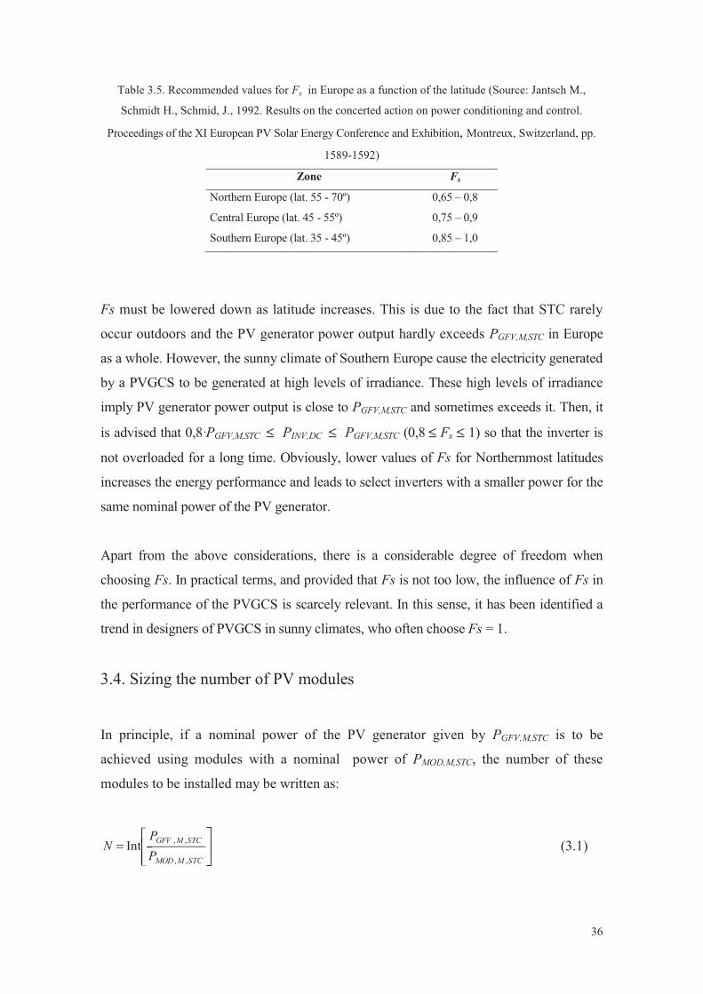
Table 3.5. Recommended values for Fs in Europe as a function of the latitude (Source: Jantsch M.,

Schmidt H., Schmid, J., 1992. Results on the concerted action on power conditioning and control.

Proceedings of the XI European PV Solar Energy Conference and Exhibition, Montreux, Switzerland, pp.

1589-1592)

Zone Fs

Northern Europe (lat. 55 - 70º) 0,65 – 0,8

Central Europe (lat. 45 - 55º) 0,75 – 0,9

Southern Europe (lat. 35 - 45º) 0,85 – 1,0

Fs must be lowered down as latitude increases. This is due to the fact that STC rarely

occur outdoors and the PV generator power output hardly exceeds PGFV,M,STC in Europe

as a whole. However, the sunny climate of Southern Europe cause the electricity generated

by a PVGCS to be generated at high levels of irradiance. These high levels of irradiance

imply PV generator power output is close to PGFV,M,STC and sometimes exceeds it. Then, it

is advised that 0,8·PGFV,M,STC PINV,DC PGFV,M,STC (0,8 Fs 1) so that the inverter is

not overloaded for a long time. Obviously, lower values of Fs for Northernmost latitudes

increases the energy performance and leads to select inverters with a smaller power for the

same nominal power of the PV generator.

Apart from the above considerations, there is a considerable degree of freedom when

choosing Fs. In practical terms, and provided that Fs is not too low, the influence of Fs in

the performance of the PVGCS is scarcely relevant. In this sense, it has been identified a

trend in designers of PVGCS in sunny climates, who often choose Fs = 1.

3.4. Sizing the number of PV modules

In principle, if a nominal power of the PV generator given by PGFV,M,STC is to be

achieved using modules with a nominal power of PMOD,M,STC, the number of these

modules to be installed may be written as:

STCMMOD

STCMGFV

PP

N,,

,,Int (3.1)

37

Eq. (3.1) is a first approach to the number of modules required, as sizing the PV

generator requires to determine the number of series connected modules or strings (Nms)

which are to be parallel connected connected (Nmp). Both figures depend on the specific

PV module and the voltage range where the inverter tracks the MPP. Additionally,

special care must be taken not to exceed the maximum input voltage of the inverter. As

shown hereafter, not always N equals Nmp · Nms. More specifically:

a) Nms must be chosen so that the sum of voltages at the MPP of all the modules

in a string lies within the voltage range where the inverter tracks the MPP in

the V-I curve of the PV generator. Nms must be sized so that the voltage at the

inverter input never exceeds the maximum voltage that this device can

withstand (VINV,M)

b) Some strings must be parallel-connected (Nmp) until the nominal power of

the PV generator is approximately achieved. Nmp must be sized so that the

current fed at the inverter input does not exceed its maximum rating

(IINV,M,DC)

3.5. Sizing the number of series-connected modules

Nms must lie within a minimum and maximum limit. The calculation of these limits is

detailed below.

3.5.1. Maximum number of series-connected modules

Low temperatures make the open circuit voltage of the PV generator increase. The most

dangerous situation may take place in a cold winter day when the inverter is

disconnected (owing to a grid failure, for example). A high voltage appears at the

inverter input that could seriously harm the device if this voltage exceeds the maximum

voltage that this device can withstand (VINV,M). Despite being conservative, a

widespread criterion assumes that the cell temperature (Tc ) may drop down to -10ºC. In

this case, the maximum number of series-connected modules that can be fed to the

inverter is given by:

38

)Cº10(,

,Int)(máxcTOCMOD

MINVms V

VN (3.2)

The PV module data sheets do not supply its open circuit voltage at Tc = -10ºC, but

these data sheets usually show the open circuit voltage temperature coefficient VMOD,OC

(usually expressed in mV·ºC-1), so that ( VMOD,OC < 0):

OCMODSTCOCMODTOCMOD VVVc ,,,)Cº70(, º·35 MVM3V7 (3.3)

If VMOD,OC is expressed in ºC-1, eq. (3.3) turns into:

)º·351( ,,,)Cº70(, OCMODSTCOCMODTOCMOD VVVc MVM3V7 (3.4)

The following approximation might be used for mono and policrystalline silicon:

STCOCMODTOCMOD VVc ,,)Cº10(, ·14,1,11 (3.5)

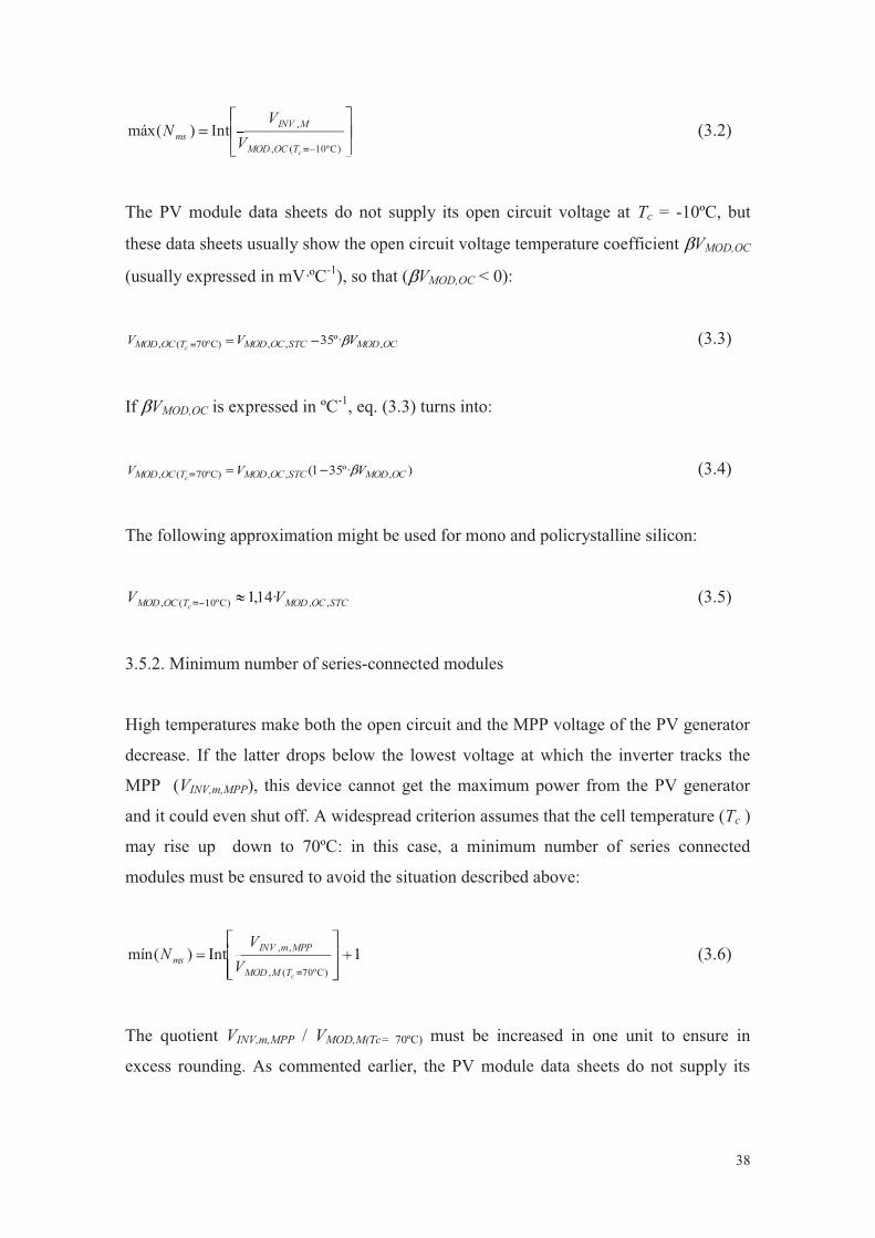
3.5.2. Minimum number of series-connected modules

High temperatures make both the open circuit and the MPP voltage of the PV generator

decrease. If the latter drops below the lowest voltage at which the inverter tracks the

MPP (VINV,m,MPP), this device cannot get the maximum power from the PV generator

and it could even shut off. A widespread criterion assumes that the cell temperature (Tc )

may rise up down to 70ºC: in this case, a minimum number of series connected

modules must be ensured to avoid the situation described above:

1Int)(mín)Cº70(,

,, 1In7cTMMOD

MPPmINVms V

VN (3.6)

The quotient VINV,m,MPP / VMOD,M(Tc= 70ºC) must be increased in one unit to ensure in

excess rounding. As commented earlier, the PV module data sheets do not supply its

39

voltage at MPP at Tc = 70ºC, but it may be calculated as follows (remember that

VMOD,OC < 0):

OCMODSTCMMODTMMOD VVVc ,,,)Cº70(, º·45 MVM4V7 (3.7)

If VMOD,OC is expressed in ºC-1, eq. (3.7) turns into:

)º·451( ,,,)Cº70(, OCMODSTCMMODTMMOD VVVc MVM4V7 (3.8)

The following approximation might be used for mono and policrystalline silicon:

STCMMODTMMOD VVc ,,)Cº70(, ·82,007 (3.8)

Figure 3.1 is addressed to clarify the above considerations and calculations. Once the

minimum and maximum number of series connected modules is ascertained, a figure

between them must be selected.

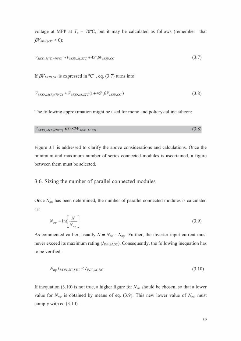
3.6. Sizing the number of parallel connected modules

Once Nms has been determined, the number of parallel connected modules is calculated

as:

msmp N

NN Int (3.9)

As commented earlier, usually N Nms · Nmp. Further, the inverter input current must

never exceed its maximum rating (IINV,M,DC). Consequently, the following inequation has

to be verified:

DCMINVSTCSCMODmp IIN ,,,, I (3.10)

If inequation (3.10) is not true, a higher figure for Nms should be chosen, so that a lower

value for Nmp is obtained by means of eq. (3.9). This new lower value of Nmp must

comply with eq (3.10).

40

V (V)

I (A

) Tc = 70ºCTc = 25ºC

Tc = -10ºC

Maximum input voltage

at the inverter input

Lowest voltage at which the inverter tracks the MPP

Inverter shut-off voltage Highest voltage at which the inverter tracks the MPP

Voltage window where the inverter tracks the PV generator MPP

Fig. 3.1. Voltage-current curves of a PV generator at different cell temperatures (Tc) and

identical irradiance (G) together with characteristic voltages of the inverter. N.B.: the second-order

influence that the cell temperature exerts on the short circuit current has been neglected in the figure

=~

. . .

. . .

…

. . .. . .

……

Fuses

Surge arresters

DC connection box

Met

al w

orks

(sup

porti

ngst

ruct

ure)

DC maincable

DC mainswitch

130,5

kWh

PV generator

Inverter

Magnetothermicswitch

Residual current circuit breaker

Grid

Earth bar

+

-

Inverterenclosure

N

L1

PE

Surge arresters

Surge arresters

Energy meter

Figure 3.2. Detailed scheme of a PVGCS (it has been assumed a single-phase inverter, although this

scheme also applies basically to a three-phase one)

41

3.7. Sizing the cabling

Figure 3.2 depicts a detailed PVGCS scheme. PV modules are series connected in

strings which are parallel connected in the DC connection box by means of cables

whose length may vary depending on how far module strings are from this box. The DC

main cable connects the DC connection box to a main DC switch located at the inverter

input. The DC main cable cross-section is obviously larger than those of the strings,

since it carries the sum of the currents that are carried by each string cable. A

magnetothermic switch is placed at the inverter output, together with a residual current

circuit breaker. Then, the electricity is fed to the grid through the energy meter device.

Regarding more detailed engineering details, each project partner must ensure that the

PVGCS complies with its national low voltage regulation code by reviewing it.

Sizing the cabling implies taking into account three crucial criteria: a) the withstand

voltage, b) the current carrying capacity and c) limiting the voltage drops through cables

at STC so that losses are minimized. Most marketed cables usually withstand voltages

up to 1000 V, which is a figure that is not exceeded in general by PV systems.

Additionally, many cables are prepared to be laid outdoors, so this does not pose any

problem in PV systems. Consequently, sizing the cables mainly implies taking into

account criteria b) and c) so that the most restrictive of them imposes the cable cross-

section to be selected.

3.7.1. Current carrying capacity

The maximum current that can flow through cables depends mostly on their cross-

section, and also on ambient temperature, their layout, if they are bundled or not, etc.

Values for the maximum currents vs. cross-section can be consulted in standard IEC

60512 part 3, although some countries have their own adapted standards (in Spain, the

standard AENOR EA 0038 applies). Additionally, IEC 60512 prescribes that PV cables

must be earth-fault proof and short-circuit proof.

42

According to IEC 60364-7-712 –at its operation temperature- each string cable must be

able to carry 1.25 times the short circuit current at STC of the string (the same current as

that of a single module) provided that fuses are available to avoid reverse currents, as

commented earlier. The same current carrying criterion applies to both the DC main

cable and the AC cable at the inverter output.

3.7.2. Limiting the voltage drops through cables at STC

Each project partner must review their national regulations concerning allowed or

recommended voltage drops at STC through cables (both in the DC and AC parts). In

the case of Spain, it is recommended a 1.5% of the voltage of the PV generator at MPP

at STC for the DC part, while not exceeding this figure for the inverter nominal output

voltage is compulsory in the AC part.

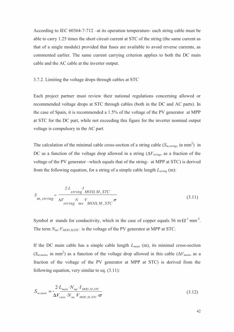
The calculation of the minimal cable cross-section of a string cable (Sm,string, in mm2) in

DC as a function of the voltage drop allowed in a string ( Vstring, as a fraction of the

voltage of the PV generator –which equals that of the string- at MPP at STC) is derived

from the following equation, for a string of a simple cable length Lstring (m):

·,,

··

,,··2

,STCMMOD

Vms

Nstring

V

STCMMODI

stringL

stringmS

V (3.11)

Symbol stands for conductivity, which in the case of copper equals 56 m· -1·mm-2.

The term Nms·VMOD,M,STC is the voltage of the PV generator at MPP at STC.

If the DC main cable has a simple cable length Lmain (m), its minimal cross-section

(Sm,main, in mm2) as a function of the voltage drop allowed in this cable ( Vmain, as a

fraction of the voltage of the PV generator at MPP at STC) is derived from the

following equation, very similar to eq. (3.11):

······2

,,

,,,

STCMMODmsmain

STCMMODmpmainmainm VNV

INLS

mVm (3.12)

43

Regarding the minimal cross-section of the cable in the AC part (Sm,AC, in mm2) as a

function of the voltage drop allowed in this part ( VAC, as a fraction of the nominal

inverter output voltage), it may be written as:

)inverter phase-isingle(··

·cos··2

,

,, ·ACINVAC

ACINVACACm VV

ILS

AVA

2 (3.13)

)inverter phase-three(··

·cos··3

,

,, ·ACINVAC

ACINVACACm VV

ILS

AVA

(3.14)

Where LAC (m) es la simple AC cable length and IINV,AC (A) is the nominal inverter

output current

3.8. Sizing some protective measures

A comprehensive review of the sizing of all required and advisable protective

measures for PVGCS lies out of the aims and scope of this document. So that it is

strongly suggested that the readers should review the sections of their national low

voltage regulation codes that deal with this important issue. Anyway, a short review of

highly advisable protective measures depicted in figure 3.2 is detailed below:

� PV modules are manufactured with built-in bypass diodes to avoid local overheatings

(hot spots) that may seriously harm the module in case of severe shadowing, cracked

cells, faulty V-I module curve, etc.

� Despite being widely used in the past, blocking diodes addressed to prevent reverse

currents have been nearly replaced by fuses completely, due to the drawbacks that

posed blocking diodes. In this sense, string cables must be protected against reverse

currents by means of gR fuses (standard IEC 60269) inserted in both poles2. These

reverse currents may take place when a string experiences an isolation fault, for

example, and they could seriously harm the string cables.

� The floating configuration is the safest one (both poles isolated from ground).

However all the metal works of the installation must be grounded. More specifically: 2 This protection is highly advised when three or more string are parallel connected

44

module frames, supporting structures, DC connection box, and metal enclosures that

house both the main DC switch and the inverter must be connected to the earth bar.

� Large area cable loops appear in PV generators, which in turn may cause voltage

surges when a lightning strike hits close to the PVGCS. Consequently, voltage surge

arresters between both positive and negative poles and earth is an advisable practice.

These devices must be installed in the DC connection box. If the distance between this

box and the inverter exceeds 10 m, they also must be installed in the inverter input,

unless this device has its own protective devices. Voltage surge arresters must be

available at the inverter output.

3.8.1. Sizing fuses

As commented above, gR fuses are housed inside the DC connection box and are series

connected to each module string. Then, string cables are protected by fuses against

reverse currents caused by faulty operation conditions. A common and widespread

criterion to determine the fuse nominal current (Ifuse) is the following one:

STCSCMODfuseSTCSCMOD III ,,,, ·22I (3.15)

So that it can be assumed that:

fuseSTCSCMOD II I,,·5,1 (3.16)

The fuse nominal current is standardized in accordance with IEC 60269. Last, fuses

must be suited for DC current and must withstand 1.1. times the open circuit voltage of

the PV generator at STC (Nms·VMOD,OC,STC).

3.8.2. DC connection box and sizing the DC main switch

Some weatherproof (IP-54 code) DC connection boxes are marketed at present so that a

limited number of strings can be easily connected in parallel with their corresponding

fuses. Voltage surge arrestors can be connected inside these boxes (see figure 1.6, in

section 1)

45

A DC main switch must be installed between the PV generator and the inverter

according to IEC 60364-7-712. This DC main switch must withstand: a) the open circuit

voltage of the PV generator at a cell temperature of -10ºC and b) 1.25 times the short

circuit current of the PV generator at STC (1,25·Nmp·IMOD,SC,STC)

3.9 Some characteristic data concerning implemented PVPPs

Two examples of real and successfully implemented PVPPs will be described hereafter

to help get an idea of the range of voltage, current, power, electricity yield, etc. that

some present state-of-the art systems deal with. Some of their features will also be

superficially discussed. Leaving aside the different levels of irradiation that can be

collected throughout Europe, it is worth saying once again that the existing huge variety

of manufactures of PV devices makes it difficult to provide some “typical” figures for

many of the above parameters.

3.9.1. A 101.2-kWp PVPP in Herreruela de Oropesa (Toledo province, Spain)

This PVPP is located in Herreruela de Oropesa (Toledo province, Spain) on an infertile

plot of land, as depicted in figure 3.3. This site has a latitude 39º 53’N, longitude 5º 14’

and height 355 m. The local meteorological conditions of the site are characterised by

an annual average daily horizontal irradiation of 4.6 kWh·m-2 together with an annual

average daily temperature of 14ºC.

The PVPP is deployed by means four ADESTM two-axis trackers -25.3 kWp-rated each-

so that the complete PV field adds up to 101.2 kWp. The latter comprises 440

SuntechTM WXS230S monocrystalline modules 230 Wp-rated each. The DC-AC

conversion is carried out by a XantrexTM GT100E 3-phase 100-kW central inverter.

This PVPP was put into commission in early 2008 and has yielded an average of 2030

kWh·kWp-1·year-1 since then. Table 3.6 gathers some characteristic electrical parameters

of the system.

46

Table 3.8. Main electrical characteristics at STC of the PV generator of the PVPP located in Herreruela de

Oropesa described in this subsection

Nominal

power

(Wp)

Series-

connected

modules

Parallel-

connected

modules

Open-circuit

voltage (V)

Short-

circuit

current (A)

Voltage at

maximum

power point (V)

Current at

maximum power

point (A)

101 200 11 40 611 226 475 212

Figure 3.3. PVPP in Herreruela de Oropesa (Toledo province, Spain). The photograph depicts on the left

a two-axis tracker of a neighbouring PVPP

3.9.2. A 9.2-MWp PVPP in Jaén (Jaén province, Spain)

The 9.2-MWp solar farm ‘Olive tree fields’ (Olivares) is located in a 16-hectare land

plot in Jaén (Jaén province, Spain, latitude 38’N, longitude 3ºW, height 520 m). This

land plot presents a nearly shadow-free skyline with negligible elevations over the

horizon. Last, a high-voltage transformer centre (20 kV / 132 kV) neighbours on the

site, so an easy access to grid connection is available.

47

The local meteorological conditions of the site are characterised by an annual average

daily horizontal irradiation of 4·9 kWh·m-2 together with an annual average daily

temperature of 16ºC.

Nearly half the above area was a garbage dump, while the other half was a low

profitable olive tree plantation, as depicted in figure 3.4. The owner of this area was not

happy either with the degraded condition of part of this area or with the low profitability

achieved by producing olive oil. Consequently, he felt enthusiastic when requested by

the future owners of the PVPP to rent out his land plot to deploy the solar farm. The

olive trees were to be pulled up and then the ground conditioned, together with that of

the neighbouring garbage dump, so as to install the PV plant.

High voltage transformer centre (20 kV / 132 kV)

Former garbage dump Former low-profitable olive tree plantation

Figure 3.4. Aerial view of the land plot prior to the deployment of the solar farm ‘Olive tree fields’

Only 220-Wp monocrystalline silicon (m-Si) modules IsofotónTM IS-220 have been

used in the solar farm ‘Olive tree fields’. Semi-fixed supporting structures allow

changing the tilt angle ranging from 15º to 35º according to the season of the year. Its

design comprises seventy two subplants rated 121·4 kWp each, together with four more

ones, rated 105·6 kWp each, adding up to seventy six subplants. The 121·4-kWp and

105·6-kWp PV fields are connected to the grid by means of IngeConTM Sun 100-kVA

and IngeConTM Sun 90-kVA 3-phase central inverters, respectively. This PVPP was put

48

into commission in August 2008 and has yielded an average slightly over 1600

kWh·kWp-1·year-1 since then. Figure 3.5. shows a partial view of the solar farm.

Figure 3.5. Partial view of the 9.2-MWp PVPP located in Jaén (solar farm ‘Olive tree fields’)

Table 3.9 gathers the layout of the PV field according to each type of subplant. Their

electrical characteristics in STC are shown in table 3.10

Table 3.9. Electrical layout of both existing types of subplant PV fields

Subplant 121·4-kWp PV field Subplant 105·6-kWp PV field

Number of modules connected in parallel 46 40

Number of modules connected in series 12 12

Table 3.10. Electrical characteristics at STC of both existing types of subplant PV fields

Parameter Subplant 121.4-kWp PV field Subplant 105.6-kWp PV field

Open-circuit voltage (V) 691 691

Short-circuit current (A) 234 204

Voltage at maximum power point (V) 553 553

Current at maximum power point (A) 219 191

Nominal power (Wp) 121 400 105 600

49

BRIEF SUMMARY OF SECTION 3

Required surface for 1-kWp PVPP if the PV modules are deployed on an

horizontal terrain surface, tilt angle slightly lower than the latitude and with no

self-shadowing between PV module arrays. Note: the figures gathered here are

somewhat overestimated. More accurate calculations for each specific latitude may

lead to smaller values of the required surface Technology Surface (m2)

Monocrystalline silicon 20

Polycrystalline silicon 27

Copper Indium Diselenide (CIS) 32

Cadmium Telluride (CdTe) 40

Sizing the nominal power of a PV generator mainly depend on two criteria. It is

up to the owner to select the most restrictive one: available area and cost of the

installed PVGCS (if attractive financial incentives are available, a more in-depth

economic analysis must be accomplished)

Sizing the inverter implies selecting a figure for the ratio between the inverter

nominal power and the PV generator nominal power. Some tables are provided for

this parameter according to the local latitude, though there is a considerable degree

of freedom when choosing a figure for it.

A PV generator is compounded of parallel-connected strings of modules. The

number of parallel-connected strings and the number of modules in a string is

driven by the inverter maximum ratings, so as the latter device is not damaged

during the normal operation of the PV generator

Sizing the cabling implies taking into account two crucial criteria: the withstand

voltage and the current carrying capacity. It is highly advised to limit the voltage

drops through cables at STC in the PV generator so that losses are minimized.

The same applies to cable losses in the AC part. Needless to say, both DC and

AC parts must comply with national electrical regulation codes

It is strongly suggested that the readers should review the sections of their

national low voltage regulation codes that deal with protective measures in PV

installations. Some of them are dealt with in this section

Leaving aside the different levels of irradiation that can be collected in each

country, the existing wide variety of manufactures of PV devices makes it

50

difficult to provide some “typical” figures for electrical characteristics of

PVPPs. Despite this, two exemplary state-of the art PVPPs have been reviewed

APPENDIX OF SECTION 3: TERMINOLOGY

IMOD,SC = Short circuit current temperature coefficient of a PV module (mA·ºC-1)

VMOD,OC = Open circuit voltage temperature coefficient of a PV module (mV·ºC-1)

VAC (adim) = Voltage drop as a fraction of the nominal inverter output voltage

Vstring (adim) = Voltage drop in a string as a fraction of the voltage of the PV generator

at MPP at STC

Vmain(adim) = Voltage drop in the DC main cable as a fraction of the voltage of the PV

generator at MPP at STC

INV,M (adim) = Maximum inverter efficiency

(m· -1·mm-2) = Conductivity

cos (adim) = Inverter power factor

f (Hz) = Frequency of the grid

Fs(adim) = Sizing factor

G (Wm-2) = Incident irradiance

GSTC (Wm-2) = Incident irradiance at STC (1000 Wm-2)

Gda (kWh·m-2 day-1) =Annual daily average daily irradiation on horizontal surface

Gda( (kWh·m-2 día-1) = PV generator on-plane annual daily average irradiation

Ifuse (A) = Nominal fuse current

IINV,AC (A) = Nominal inverter output current

IINV,M,DC (A) = Inverter input maximum DC current

IMOD,M,STC (A) = PV module current at MPP at STC

IMOD,SC,STC (A) = PV module short-circuit current at STC

LAC (m) = AC cable simple length

Lmain (m) = DC main cable simple length

Lstring (m) = String cable simple length

N (adim) = Total number of modules of the PV generator

Ncs (adim) = Series connected cells in a module

Ncp (adim) = Parallel connected cells in a module

51

Nmp (adim) = Parallel connected number of strings

Nms (adim) = Series connected PV modules in a string

NOCT (ºC) = Nominal operation cell temperature (ºC)

PGFV,M,STC (Wp) = Maximum power of a PV generator at STC or nominal power of a PV

generator

PINV,AC (W) = Inverter output nominal power

PINV,DC (W) = Inverter input nominal power

PMOD,M,STC (Wp) = Maximum power of a PV module at STC or nominal power of a PV

module

PR (adim.) = Performance ratio

Sm,AC (mm2) = Minimal cable cross-section of an AC cable as a function of the allowed

voltage drop

Sm,main. (mm2) = Minimal cable cross-section of the DC main cable (Sm,string, in mm2) as a

function of the allowed voltage drop

Sm,rstring (mm2) = Minimal cable cross-section of a string cable as a function of the

allowed voltage drop

Ta (ºC) = Ambient temperature

Tc (ºC) = Cell temperature

VINV,AC (V) = Inverter output nominal voltage

VINV,M (V) = Inverter input maximum voltage

VINV,m,MPP (V) = Lowest voltage at which the inverter tracks the MPP of the PV

generator

VINV,M,MPP (V) = Highest voltage at which the inverter tracks the MPP of the PV

generator

VMOD,M,STC (V) = PV module voltage at MPP at STC

VMOD,OC,STC (V) = PV module open circuit voltage at STC

52

4. Matching PVPP Typologies to Specific Terrains

Given the wide variety of existing PVPP system typologies and the numerous

peculiarities that characterize a marginal terrain type, providing some guidance to assess

which PVPP system typologies may suit best a specific marginal terrain type could be

found useful. Thus, a specific multivariable table might be completed using this

guidance. The following text has been extracted from the Strategic Vision Document

Rocky, sandy or subsidency terrain consistency is not advisable for any PVPP typology.

Obviously, terrains with risk presence –geological, hydro or seismic- should be rejected.

Regarding cliviometry, high land slope -above 5%- hinders the deployment of PVPP

that use tracking techniques, but under certain boundaries, high land slope is a neutral

item in the case of static and semi static modules.

Terrains with indented surfaces must be avoided: this is a powerful barrier for the

necessary civil works to deploy a PVPP. Additionally, subsequent operation and

maintenance turns into a difficult task. Wet or waterlogged grounds do not pose an

obstacle for PVPPs. Regular surfaces are obviously the preferred ones.

As it may be easily understood, sites with high irradiation profiles will lead to a

substantial solar electricity production. Terrains with an annual average horizontal

irradiation below 900 kWh/m2 should be disregarded. If concentrator photovoltaic

(CPV) is to be installed, at least some annual average normal direct irradiation of 1800

kWh/m2 is required.

Severe shadowing should certainly be avoided, but energy losses caused by tiny

shadowing at the down and sunset in winter are negligible: in this case, the terrain

would be acceptable.

Solar cell performance benefits from cooling through forced convection by means of

wind, so in the case of static and semi static PVPP, moderate windy areas (maximum

wind speed of some 30-40 km/h) favour solar electricity production. However, highly

windy zones (frequent wind peaks above 60 km/h) are not suitable for PVPP that use

tracking techniques. In such zones, at best, the tracking systems will frequently change

53

their operation to the stow position and the energy yield will be negatively affected. At

worst, some of these systems can be seriously damaged.

The negative effect of dust was underestimated in PVPPs in the past. Recent studies

prove that energy losses up to some 15-20% might take place due to dust and dirtiness.

Consequently, dusty marginal terrains should be avoided. Besides, special attention

must be paid to the neighbouring areas of the marginal terrain where the PVPP is to be

deployed. For instance, arable surrounding areas in dry climates are not advisable.

If the marginal terrain climate is not too cloudy –this would affect the annual average

horizontal irradiation- rain may help to keep the PV modules clean. Consequently,

moderate monthly average rainfall values (5-7 cm) are beneficial for any PVPP

typology.

Easy access to grid connection is highly advisable.

Easy road access to the marginal area is advisable for two reasons. First, transportation

of all the necessary material to deploy any PVPP will be much easier and less costly.

The same applies to the operation and maintenance tasks to be carried out through the

useful life of the PVPP.

Communication coverage –Internet access availability, GPRS, etc- is increasingly

becoming important. Electric companies –which in the end, buy the generated

electricity- usually force owners of large and relatively isolated PVPP in marginal

terrains to provide remote access to their energy meters

BRIEF SUMMARY OF SECTION 4

There is wide variety of possible PVPP system typologies whilst the peculiarities

that characterize a marginal terrain type are numerous. This turns matching the

former with the latter into a cumbersome task when approached using

multivariable tables.

54

This section is aimed at providing some guidance to assess which PVPP system

typologies may suit best a specific marginal terrain type.

55

5. Economic assessment on PV Grid-Connected systems On-ground photovoltaic grid–connected systems (PVGCS) are becoming the most

popular application of the photovoltaic technology in developed countries. This is

mainly due to the governmental support programmes and policies launched by these

countries and a continuous decrease trend in photovoltaic (PV) cost. These policies are

implemented with financial incentives broadly fall into investment-focused (initial

investment subsidy, soft loans, income tax incentives, etc.) and generation-based (feed-

in tariffs (FIT), net metering, etc.) ones.

Firstly, in this section some available supporting measures for PVGCS and indicative

installed system prices of them in each project partner country are shortly reviewed.

Besides, some profitability indices of investment project applied of PVGCS have been

reviewed. More specifically, the internal rate of return (IRR), that provides some

straightforward meaningful information for the investor of these PV systems.

Estimation the IRR must be solved through non-analytical methods. This is why some

easy-to-use tables addressed to estimate the value of IRR are proposed in this section.

Finally, in this section it has been carried out an economic analysis of the PVGCS,

through the profitability index IRR. This analysis provides some figures for the IRR that

may enlighten a prospective PVGCS owner decision. In this analysis, for the sake of

simplicity, only initial investment subsidy, soft loans for the whole remaining initial

cost after the initial investment subsidy to be repaid in equal annual installments, feed-

in tariffs and the annual increase rate of the PV electricity price are considered in a first

approach for three specific cases (cases A, B and C, from now on) of possible

investments on PVGCS. In these cases, the effect of taxation has not been considered.

However, as ignoring completely the tax influence may lead to unrealistic results, a

brief analysis concerning the impact of taxation in these three cases (A,B and C) is

carried out. Last, some figures of IRR are shown for some cases of PVGCS with the

same initial investment and different financial incentives (soft loans, initial investment

subsidy and feed-in tariffs).

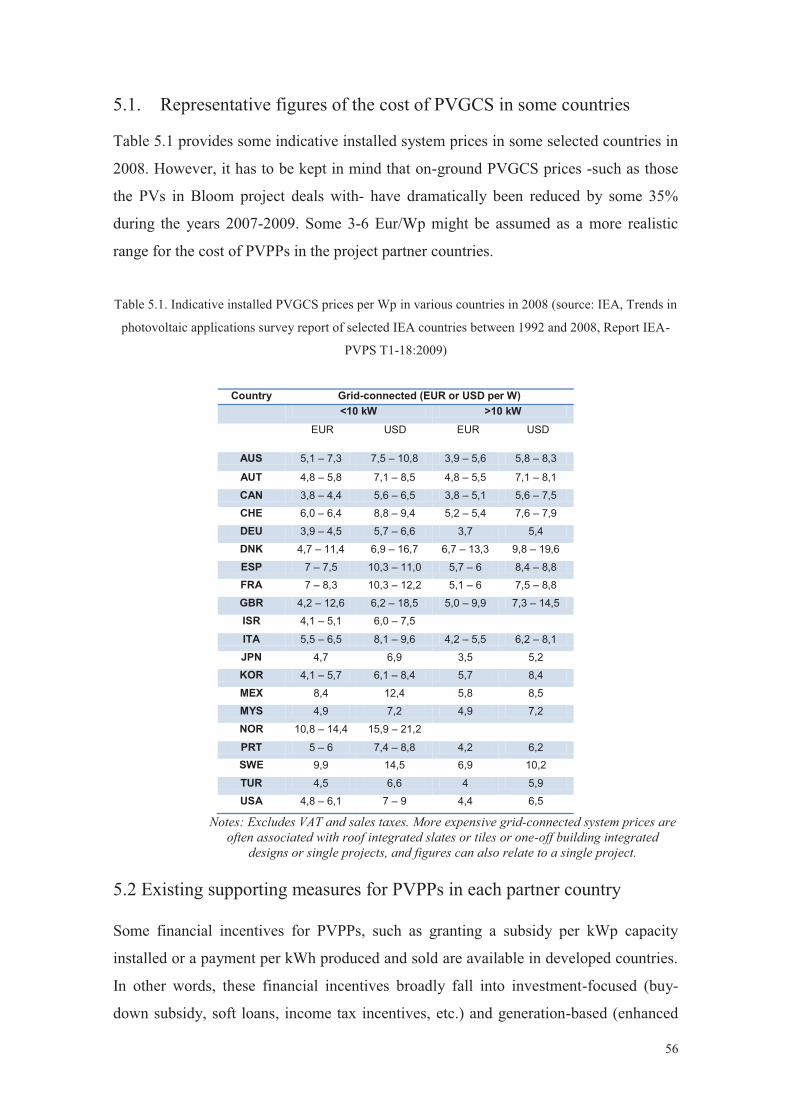
56

5.1. Representative figures of the cost of PVGCS in some countries

Table 5.1 provides some indicative installed system prices in some selected countries in

2008. However, it has to be kept in mind that on-ground PVGCS prices -such as those

the PVs in Bloom project deals with- have dramatically been reduced by some 35%

during the years 2007-2009. Some 3-6 Eur/Wp might be assumed as a more realistic

range for the cost of PVPPs in the project partner countries.

Table 5.1. Indicative installed PVGCS prices per Wp in various countries in 2008 (source: IEA, Trends in

photovoltaic applications survey report of selected IEA countries between 1992 and 2008, Report IEA-

PVPS T1-18:2009)

Country Grid-connected (EUR or USD per W)

<10 kW >10 kW

EUR USD EUR USD

AUS 5,1 – 7,3 7,5 – 10,8 3,9 – 5,6 5,8 – 8,3

AUT 4,8 – 5,8 7,1 – 8,5 4,8 – 5,5 7,1 – 8,1

CAN 3,8 – 4,4 5,6 – 6,5 3,8 – 5,1 5,6 – 7,5 CHE 6,0 – 6,4 8,8 – 9,4 5,2 – 5,4 7,6 – 7,9

DEU 3,9 – 4,5 5,7 – 6,6 3,7 5,4 DNK 4,7 – 11,4 6,9 – 16,7 6,7 – 13,3 9,8 – 19,6

ESP 7 – 7,5 10,3 – 11,0 5,7 – 6 8,4 – 8,8 FRA 7 – 8,3 10,3 – 12,2 5,1 – 6 7,5 – 8,8

GBR 4,2 – 12,6 6,2 – 18,5 5,0 – 9,9 7,3 – 14,5 ISR 4,1 – 5,1 6,0 – 7,5 ITA 5,5 – 6,5 8,1 – 9,6 4,2 – 5,5 6,2 – 8,1

JPN 4,7 6,9 3,5 5,2 KOR 4,1 – 5,7 6,1 – 8,4 5,7 8,4

MEX 8,4 12,4 5,8 8,5 MYS 4,9 7,2 4,9 7,2

NOR 10,8 – 14,4 15,9 – 21,2 PRT 5 – 6 7,4 – 8,8 4,2 6,2 SWE 9,9 14,5 6,9 10,2

TUR 4,5 6,6 4 5,9 USA 4,8 – 6,1 7 – 9 4,4 6,5

Notes: Excludes VAT and sales taxes. More expensive grid-connected system prices are often associated with roof integrated slates or tiles or one-off building integrated

designs or single projects, and figures can also relate to a single project. 5.2 Existing supporting measures for PVPPs in each partner country Some financial incentives for PVPPs, such as granting a subsidy per kWp capacity

installed or a payment per kWh produced and sold are available in developed countries.

In other words, these financial incentives broadly fall into investment-focused (buy-

down subsidy, soft loans, income tax incentives, etc.) and generation-based (enhanced

57

feed-in tariffs (FIT), net metering, etc.) ones. More specifically, some PV financial

incentives are detailed below:

Feed-in tariff: an explicit monetary reward is provided for producing PV

electricity; paid (usually by the electricity utility) at a rate per kWh somewhat

higher than the retail electricity rates being paid by the customer.

Capital subsidies: direct financial subsidies aimed at tackling the up-front cost

barrier, either for specific equipment or total installed PV system cost.

PV-specific green electricity schemes: allows customers to purchase green

electricity based on PV electricity from the electricity utility, usually at a

premium price.

Income tax credits: allows some or all expenses associated with PV installation

to be deducted from taxable income streams.

Commercial bank activities (Low-interest loans): includes activities such as

preferential home mortgage terms for houses including PV systems and

preferential green loans for the installation of PV systems.

Net metering: in effect the system owner receives retail value for any excess

electricity fed into the grid, as recorded by a bi-directional electricity meter and

netted over the billing period.

Net billing: the electricity taken from the grid and the electricity fed into the grid

are tracked separately, and the electricity fed into the grid is valued at a given

price.

In general, the last two financial incentives do not apply to PVPPs as all the PV-

generated electricity is fed and sold to the grid. More concretely, some available

supporting measures for PVGCS in each project partner country are shortly reviewed

below:

Austria The Ökostromverordnung 2009 (eco electricity degree) set the following new tariffs for

2009 (only for PV systems covered by the Ökostromgesetz (Eco Electricty Law).

■ System size < 5 kW: 0.4598 €/kWh

■ System size 5 to 10 kW: 0.3998 €/kWh

■ System size > 10 kW: 0.2998 €/kWh

58

For installations supported under the feed-in tariff scheme, 100 % of the specific tariff is

paid for the first 10 years. Afterwards, the tariff is cut to 75 % in year 11 and finally 50

% in year 12. After this period, only the gross sale price for electricity is paid. Some of

the Federal States have additional investment support schemes.

Greece

In January 2009 a new feed-in-tariff regime was introduced in Greece. The tariffs will

remain unchanged until August 2010 and are guaranteed for 20 years. However, if a

grid connection agreement is signed before that date, the unchanged FIT will be applied

if the system is finalized within the next 18 months.

Already filed applications for permits (> 3 GW) had to be served until the end of 2009.

The regime for new applications is not yet known.

Feed-in tariff [€/kWh]:

Start of operation Mainland Grid Autonomous island grids

> 100 kWp ≤ 100 kWp > 100 kWp ≤ 100 kWp

February 2009: 0.40 0.45 0.45 0.50

August 2009: 0.40 0.45 0.45 0.50

February 2010: 0.40 0.45 0.45 0.50

August 2010: 0.392 0.441 0.441 0.49

From then on the degression of the tariffs for new systems will be 5% each half year.

A 40% grant will still be available on top of the new FITs for most of the systems

(minimum investment eligible for grant is € 100,000).

New since 4 June 2009: rooftop PV systems up to 10 kWp (both for residential users

and small companies) receive 0.55 €/kWh. Annual degression of 5% is foreseen for

newcomers as of 2012. This does not apply to PVPPs, obviously.

Regarding changes of PV’s legislation, the pricing of electricity produced by

photovoltaic power is based on the data shown in Table 5.2

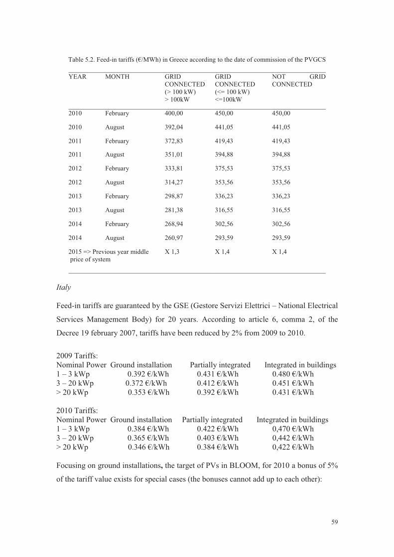
59

Table 5.2. Feed-in tariffs (€/MWh) in Greece according to the date of commission of the PVGCS

YEAR MONTH GRID

CONNECTED (> 100 kW)

GRID CONNECTED (<= 100 kW)

NOT GRID CONNECTED

> 100kW <=100kW

2010 February 400,00 450,00 450,00

2010 August 392,04 441,05 441,05

2011 February 372,83 419,43 419,43

2011 August 351,01 394,88 394,88

2012 February 333,81 375,53 375,53

2012 August 314,27 353,56 353,56

2013 February 298,87 336,23 336,23

2013 August 281,38 316,55 316,55

2014 February 268,94 302,56 302,56

2014 August 260,97 293,59 293,59

2015 => Previous year middle price of system

X 1,3 X 1,4 X 1,4

Italy Feed-in tariffs are guaranteed by the GSE (Gestore Servizi Elettrici – National Electrical

Services Management Body) for 20 years. According to article 6, comma 2, of the

Decree 19 february 2007, tariffs have been reduced by 2% from 2009 to 2010.

2009 Tariffs: Nominal Power Ground installation Partially integrated Integrated in buildings 1 – 3 kWp 0.392 €/kWh 0.431 €/kWh 0.480 €/kWh 3 – 20 kWp 0.372 €/kWh 0.412 €/kWh 0.451 €/kWh > 20 kWp 0.353 €/kWh 0.392 €/kWh 0.431 €/kWh 2010 Tariffs: Nominal Power Ground installation Partially integrated Integrated in buildings 1 – 3 kWp 0.384 €/kWh 0.422 €/kWh 0,470 €/kWh 3 – 20 kWp 0.365 €/kWh 0.403 €/kWh 0,442 €/kWh > 20 kWp 0.346 €/kWh 0.384 €/kWh 0,422 €/kWh Focusing on ground installations, the target of PVs in BLOOM, for 2010 a bonus of 5%

of the tariff value exists for special cases (the bonuses cannot add up to each other):

60

in the case of a ground system where the 70% of the electricity is used up

directly by the producer or societies controlled by the producer

for plants that are owned by a public school or public health structure

for plants which are owned by local administrations with less than 5.000

inhabitants

Reduction of VAT from 20% to 10%

The incentive rates are combined with certain public benefits and contributions

(capital contributions up to 30% of investment cost) and the soft loans of 0.50%

under the Kyoto Fund (Article 1, paragraph 1111, 2007 Financial Law).

Enjoying the reduction of VAT cannot combine with tax deductions.

For 2011 the Government has announced the possibility of cutting back the tariffs by

another 20% maximum. Such percentage is currently under discussion by the Italian

Ministry for Economic Development and stakeholders from the PV national industry,

and it seems that the parties are reaching a compromise around a solution that could

foresee a gradual reduction of the tariff by 6% every 4 months, following the German

model.

Therefore, the installations connected to the grid by April 2011 could have tariff

reductions among 6.5 to 8.1%; those between April and August from 10% and 12.8%,

while those between August and December 2011 among 15% and 17.6%.

Also under discussion, for ground PV plants, is the bonus of 5% for installations in

marginal areas (the proposal of Decree mentions exhausted quarries, areas of relevance

to landfills, etc.).

Another 6 or 8% should be cut back every year starting from 2012. Innovative plants

could however benefit from a lower cut back (around 2% every year).

That of ‘innovative plants’ (the category ‘integrated photovoltaic systems with

innovative features’) is a novelty that has been recently introduced and will benefit from

incentive rates (divided in three intervals of power) higher than the other categories. The

61

tariffs for “innovative plants” could be cut by 2% per year (instead of 6%) in 2012 and

2013. By 1 January 2011, the GSE will develop a guide on the features that these

innovative systems must have.

Also an increase in the total power for which incentives can be provided is under

discussion: it is foreseen that the ceiling will be raised from 2,000 MW in 2015 and

3,000 MW in 2016, with other 150 MW added for additional installations of plants with

concentration technology. The objective of national power to be installed by 2020 is set

at 8,000 MW.

Another change foreseen is the division of power plants in 5 classes: between 1 and 3

kW, between 3 to 20 kW, between 20 and 200 kW, between 200 to 1000 kW and over

1000 kW.

Moreover, welcoming the suggestion of producers to simplify the types of installation

(removing the category of partially integrated plants) the draft ministerial decree

foresees only two types: ‘photovoltaic systems integrated in buildings’ and ‘other

photovoltaic installations’

Poland

There is no Feed in Tariff in Poland at this moment. Legislation considering Legislation

considering Energetic Law (Regulation of Minister for the Economy Coll. U. Nr 122,

poz. 1336, dated 15 December 2000; http://www.ure.gov.pl/portal.php?serwis=

pl&dzial= 195&id=882& search=25421) makes an obligation to the government to buy

any amount of green energy without any quantity restrictions. For selling such energy,

the producer is granted ‘a green certificate’ which is sold in the stock exchange. The

average price of the green certificate equals 0.26 PLN/kWh (0.07 €cent/kWh1).

As a result of actions taken under the ‘PVs in Bloom’ project in Lublin’s region some

subsidies were introduced for those who want to invest on renewable energies.

Amount of subsidies for local governments is 3 million PLN for each investment.

1 Exchange rate: 1 € = 3.88 PLN

62

Spain Financial incentives applied to PVGCS at present (royal decree 1578/2008) are briefly described below: Installation types:

1.1. Systems in or on top of buildings with at most 20kW power

1.2. Systems in or on top of buildings with more than 20kW of power

2. Systems on undeveloped areas

Systems installed on the ground with more than 10MW and rooftop systems with more

than 2MW of power will not receive feed-in tariffs.

Cap for every type of installation (per year but quarterly sufficed):

1.1. 26.7MW

1.2. 240.3MW

2. 133MW, with an additional 100MW of installed power in 2009 and 60MW in

2010.

Tariffs (paid over 25 years):

1.1. 34 euro cents/kWh

1.2. 32 euro cents/kWh

2. 32 euro cents/kWh

Changes to the cap and tariff rates:

If at least 75% of a particular quarterly cap is exhausted, the tariff for the corresponding

installation type is decreased by at most 2.5%, while at the same time the amount of

available installable power is increased by the same amount.

If less than 50% of a cap is exhausted, the corresponding tariff increases, while the cap

decreases by an equal amount (without consideration of addition power). If the cap is

exhausted by between 50 and 75%, the tariffs and the amount of installable power

63

remains the same. Adjustments for installable power will be made on an annual basis

and the tariffs will be adjusted quarterly.

Slovakia Feed-in tariff is set by Regulator each year. The new feed-in tariff for 2009 is 13.2

SKK/kWh (0.434 €/kWh2) guaranteed for 12 years. In addition, PV, like all other RES,

qualifies for investment subsidies under the framework of the EU Structural funds.

2 Exchange rate: 1 € = 30.396 SKK

5.3 Review of the most meaningful and understandable profitability indices: the internal rate of return (IRR) 5.3.1. Introduction

From a strictly economic viewpoint, the purchase of a PVPP means an expenditure of

capital resources at a given time with the expectation of benefits in the form of solar

electricity yield to be paid/saved to/by the user over the useful life of the system.

As commented in other sections of this document, many financial mechanisms are

available in developed countries intended to promote PVPPs. However, for the sake of

simplicity, only initial investment subsidy, soft loans for the whole remaining initial

cost after the initial investment subsidy to be repaid in equal annual installments, feed-

in tariffs and the annual increase rate of the PV electricity price are considered in a first

approach for three specific cases (cases A, B and C, from now on) of possible

investments on PVPPs, leaving aside the effect of taxation. However, as ignoring

completely the tax influence may lead to unrealistic results, a brief analysis concerning

the impact of taxation in these three cases puts an end to this study.

5.3.2. A review of four profitability indices The simple payback time (SPBT) of an investment project is the required number of

years for the inflows to equal the outflows of this project. Despite being easily

understandable, this profitability index does not take into account the moment over the

life of the project when these inflows and outflows take place, so it is a rather unrealistic

64

index (e.g.: a 3,000-Euro income in 2009 has more worth than a 3,000-Euro income in

2019). In this sense, it is preferred to deal with the discounted payback time (DPBT),

stated as the required number of years for the present worth of the inflows to equal the

present worth of the outflows (the present worth implies using an annual discount rate

and taking into account the annual inflation rate). Evidently, profitability means that the

discounted payback time should not exceed the serviceable life of the system. Although

it is also easily understandable and straightforward, this parameter does not consider the

cash flows that are produced after the DPBT. Hence, it may hide sound financial

opportunities for those deciding to invest on a PV system3.

The net present value (NPV, in €) of an investment project is the sum of present values

of all cash inflows (PW[CIF(N)], in €, where N is the useful life of the PV system, in

years) and outflows related to the investment4 . Therefore, the parameter NPV equals the

present worth of the cash inflows from the system minus the life-cycle cost from the

user standpoint (LCCUSP). Thus:

USPLCCNNPV L)(CIFPW (5.1)

Obviously, a PVGCS should be viewed favourably if NPV > 0. However, this parameter

fails to choose among two projects with the same NPV but different initial costs and

duration.

The internal rate of return (IRR) of an investment project equals the actual interest rate

at which the project initial investment should be lent during its useful life to achieve the

same profitability5. Also, the internal rate of return (IRR) of an investment project is the

value of the interest rate that leads to NPV = 0. This is to say:

0)(CIFPW 0P USPLCCNNPV (5.2)

3 Perez R, Burtis L, Hoff T, Swanson S, Herig C. Quantifying residential PV economics in the US-payback vs cash flow determination of fair energy value. Solar Energy 2004;77:363-366. 4 Lasnier F, Ang T. Photovoltaic engineering handbook. Great Yarmouth: Adam Hilger; 1990. p. 371-399. 5 Chabot B. From cost to prices: economic analysis of photovoltaic energy and services. Progress in Photovoltaics: Research and Applications 1998;6:55-68.

65

From an economic point of view, the PV system should be accepted if the IRR exceeds

a profitability threshold fixed by the future owner. In this sense, this parameter is very

important for the investor since it provides a meaningful estimation of the return of their

investment. The actual internal rate of return (IRRa) is derived from IRR by IRRa= (IRR-

g)/(1+g), where g is the annual inflation rate.

The value of the internal rate of return (IRR) for a given PV system, may be calculated

through both parameters LCCUSP and PW[CIF(N)]. When the life-cycle cost of the

system from the user standpoint and the present worth of cash inflows from the system

are equal, at the same value of d, the solution is found (IRR = d).

5.4 Easy-to-use tables to estimate the IRR Unfortunately, equation (5.2) must be solved through non-analytical methods. This is

why some easy-to-use tables addressed to estimate the value of IRR are proposed in this

subsection (see Annex enclosed to this section). In fact, the internal rate of return (IRR)

equals the value of discount rate d that verifies equation (5.2). Values of IRR > 0 will be

feasible solutions from an economic point, provided that a certain profitability hurdle

set by the investor is reached.

Tables are used following the steps detailed below:

1. Choose the tables for the calculation of LCCUSP, according to the type of loan –if any,

this is determined by the loan interest (il) and the loan duration (Nl)- addressed to partly

finance the initial investment. For the specific values of the initial investment (PVIN)

and the initial buy-down or subsidy (PVIS), find a group of values LCCUSP for several

values of discount rate d. Choose a value of d so that from this value of d, it follows a

value of LCCUSP.

2. Choose the tables for the calculation of PW[CIF(N)], according to the annual increase

rate of energy price ( pu). For the specific values of EPV and pu, find a group of values

PW[CIF(N)] for several values of discount rate d. Also choose the same value of d that

was chosen in step 1. Select the corresponding value of PW[CIF(N)].

3. Substract PW[CIF(N)] minus LCCUSP

4. Three cases may appear depending on the result of step 3:

66

4.1. If the result of step 3 is equal to zero, then IRR = d.

4.2. If the result of step 3 is negative, the discount rate d that is sought has a lower value

than that chosen in step 1. Therefore, return to step 1 and choose the nearest lower value

of d in this column. Iterations are continued until the difference obtained in step 3 turns

into positive. Then, the solution is found: the value of IRR lies within the values of d of

the last two iterations. The difference obtained in step 3 might not turn into positive at

the lowest value of d = 0·01 considered in the tables. This would mean that the PVGCS

project should be rejected since IRR < 0.

4.3. If the result of step 3 is positive, the discount rate d that is sought has a higher value

than that chosen in step 1. Therefore, return to step 1 and choose the nearest higher

value of d in this column. Iterations are continued until the difference obtained in step 3

turns into negative. Then, the solution is found: the value of IRR lies within the values

of d of the last two iterations. The difference obtained in step 3 might not turn into

negative at the highest value of d considered in the tables. In this case, the tables only

provide a lower bound for IRR which is equal to the last tried value of d.

5.4.1 Some examples Giving a tutorial on how to calculate the IRR lies out of the scope of this document, but

the method to do this may be found in literature6,7. Nevertheless, providing some figures

for this profitability index in three specific cases may enlighten a prospective PVPP

owner decision. In this sense, some factors are involved in the calculation of the IRR

and -as it can easily be anticipated- they are mainly related to costs, incentives,

electricity yields and the annual increase rate of the PV electricity price. Finally, in

Table 5.3 are presented values of IRR for some cases of PVGCS with the same initial

investment and different financial incentives (soft loans, initial investment subsidy and

feed-in tariffs). The figures that configure each one of the three cases mentioned earlier

which refer to costs, incentives and electricity yields are commonly normalised-per-

6 Talavera DL, Nofuentes G, Aguilera J, Fuentes M. Tables for the estimation of the internal rate of

return of photovoltaic grid-connected systems. Renewable & Sustainable Energy Reviews 2007; 11:447-

466. 7 Nofuentes G, Aguilera J. and Muñoz FJ. Tools for the Profitability Analysis of Grid-Connected

Photovoltaics. Progress in Photovoltaics: Research and Applications, 2002;10:555-570.

67

kWp. Some values that characterize each one of the cases are given below, together

with the corresponding figure for the IRR:

Case A: The normalised annual PV electricity yield ([EPV]kWp) is assumed equal to 1400

kWh kWp-1 year-1 .

The normalised initial investment in the PVGCS ([PVIN]kWp) is assumed equal to

6000 € kWp-1 .

The corresponding price per kWh for PV-generated electricity sold to the grid

(pu), is fixed by law in different countries. It is assumed equal to 0.30 € kWh-1

The annual increase rate of the PV electricity price ( pu) is assumed equal to 2%.

The normalised initial investment subsidy ([PVIS]kWp) is assumed equal to 17% of

[PVIN]kWp therefore [PVIS]kWp is assumed equal to 1000 €·kWp-1. It is worth

mentioning some countries provide capital subsidies ranging from 10 to 50

percent 8,9.

Consequently, the remaining sum [PVIN]kWp–[PVIS]kWp is to be paid by the owner.

This amount is assumed to be borrowed at an annual loan interest il= 5% while the

loan term Nl is assumed equal to 10 years.

Use of the tables provided in the annex for this example:

1.- From table 2, column 4 (6000 € kWp-1 ) and rows where [PVIS]kWp = 1000 €·kWp-1

are considered. Let us choose a value of d = 0·09, so that [LCCUSP]kWp = 4745 €·kWp-1 .

2.- From table 5, column 5 and rows where pu = 0·3 €·kWh-1 are considered. It follows

from the row corresponding to the same value of d = 0·09 that PW[CIF(N)]]kWp= 4956

€·kWp-1.

3.- Let us subtract 1-·kWp€211)(CIFPW 2USP

LCCN .

4.-Since USPLCCN L)(CIFPW > 0, parameter IRR has a higher value. Therefore, let us

8 Martinot E. Renewable: Global status report. REN21 Renewable Energy Policy Network by The

Worldwatch Institute, 2005. Available

at:http://www.martinot.info/RE2005_Global_Status_Report.pdf(accessed November 2006). 9 Martinot E. Renewable: Global status report, Update. REN21 Renewable Energy Policy Network, 2006. Available at:http://www.ren21.net/globalstatusreport/download/RE_GSR_2006_Update.pdf (accessed September 2007).

68

return to step 1 and try with d = 0·11.

1.- From table 2, column 4 and rows where [PVIS]kWp = 1000 €·kWp-1 are considered

again. Let us choose a value of d = 0·11, so that [LCCUSP]kWp = 4319 €·kWp-1 .

2.- From table 5, column 5 and rows where pu = 0·3 €·kWh-1 are considered again. It

follows from the row corresponding to the same value of d = 0·11 that

PW[CIF(N)]]kWp= 4185 €·kWp-1.

3.- Let us subtract 1-·kWp€134)(CIFPW 1USP

LCCN .

4.- Since the difference obtained in step 3 turns into negative, the solution is found: the

value of IRR lies within 9-11%.

IRR in case A lies within a very attractive 9 - 11%. Let us choose a value of IRR=9% (most

unfavorable case).

Case B:

[EPV]kWp is assumed equal to 1200 kWh kWp-1 year-1.

[PVIN]kWp is assumed equal to 5000 € kWp-1.

The corresponding price per kWh for PV-generated electricity paid/saved to/by

the owner (pu) is assumed equal to 0.20 € kWh-1.

pu is assumed equal to 2% .

[PVIS]kWp is assumed equal to 1500 € kWp-1.

Consequently, the remaining sum [PVIN]kWp–[PVIS]kWp is to be paid by the owner.

This amount is assumed to be borrowed at an annual loan interest il= 5%, while the

loan term Nl is assumed equal to 20 years.

Tables 3 and 5 provided in the annex should be used for the calculation of LCCUSP and

PW[CIF(N)]. If the procedure described for case A is followed, IRR in case B equals an

attractive 5 - 7%. Let us choose a value of IRR=5% (most unfavorable case).

Case C:

[EPV]kWp is considered equal to 1000 kWh kWp-1 year-1 .

[PVIN]kWp is assumed equal to 4000 € kWp-1 .

The corresponding price per kWh for PV-generated electricity paid/saved to/by

the owner (pu) is assumed equal to 0.20 € kWh-1.

69

pu is assumed equal to 1%.

[PVIS]kWp is assumed equal to 25% of [PVIN]kWp, therefore [PVIS]kWp is assumed

equal to 1000 € kWp-1 [7,9].

Consequently, the remaining sum [PVIN]kWp–[PVIS]kWp is to be paid by the owner.

This amount is assumed to be borrowed at annual interest rate il= 5% over a term

equal to Nl= 20 years.

Tables 3 and 4 provided in the annex should be used for the calculation of LCCUSP and

PW[CIF(N)]. IRR in case C equals a fairly good 3 - 5%. Let us choose a value of IRR=3%

(most unfavorable case).

The analysis of some other cases may help achieve a better understanding. Table 5.3 shows values the IRR for PV Grid-Connected Systems with same initial investment and different support measures.

Table 5.3. IRR for PVGCS with the same initial investment and different financial incentives.

[EPV]kWp

(kWh kWp-1 year-1)

[PVIN]kWp

(€ kWp-1)

pu

(€ kWh-1)

pu

(%)

[PVIS]kWp

(€ kWp-1)

Soft loans

Nl (years) il (%)

IRR

(%)

1200 4000

0.2

2

1000 No available 5-7

Nl=10 il=5 7-9

Non available Nl=10 il=5 3-5

0.3 Non available Non available 5-7

1400 0.2 Non available Non available 5-7

5.5. Short review of the taxation impact As commented previously, the above cases have ignored the tax influence. However,

some basic issues concerning this influence will shortly be dealt with below to help

achieve an approach that tries not to conceal the effect of taxation. Anyway, it should be

kept in mind that the general assumptions that follow are reasonable, but taxation differs

considerably from country to country. However, tax exemptions have been left aside,

due to the wide differences concerning this issue also from country to country.

70

In general, most existing tax laws, consider that every owner of a PVPP must pay an

amount per annum, mostly attributable to the gains of the previous year. This amount

depends on the law defined tax coefficient, investment revenue, the annual operation

and maintenance cost, the debt repayment method, the asset amortization, etc.

The diversity of taxation systems according to each country makes it complex to

encompass this issue in our analysis. Anyway, several tax coefficient values -ranging

from 0% up to 40%- have been considered.10 In this subsection an analysis of the IRR

has been made by means of taking into account a tax coefficient, for the three

considered cases. In order to estimate the taxes, this coefficient has been applied to the

cash inflow from the PVPP, once the asset amortization, the interest payments of the

loan, and the operation and maintenance cost of the PVGCS are deducted. The asset

amortization has been considered lineal over the life cycle of the PVPP (25 years) and it

has been excluded from taxation. The results of the analysis in the base cases for

scenarios A, B and C are shown in figure 5.4. In this figure, the internal rate of return is

depicted vs the percentage tax coefficient. The IRR experiences a smooth and almost

linear decrease as the taxation coefficient increases. More specifically, when the latter

rises to 40%, the former is only decreased by 2.7% for case A, 1.4% for case B and

0.8% for case C.

10 Kaldellis JK, Vlachou DS, Korbakis G. Techno-economic evaluation of small hydro power plants in Greece: a complete sensitivity analysis. Energy Policy 2005;33:1969-1985.

71

Figure 5.4. IRR (%) as a function of the percentage tax coefficient values for cases A (uppermost line), B (medium line) and C (lowermost line)

72

BRIEF SUMMARY OF SECTION 5 A continuous decrease trend in PV costs together with a wide variety of supporting

measures have turned photovoltaic grid-connected systems (PVGCS) into a

profitable investment when some economic conditions are met.

On-ground PVGCS prices -such as those the PVs in Bloom project deals with- have

dramatically been reduced by some 35% during the years 2007-2009. Some 3-6

Eur/Wp might be assumed as a realistic range for the cost of PVPPs in the project

partner countries.

In Europe, different forms of financing for PVGCS have been defined and put into

effect in the last years. The most popular one in Europe are the feed-in tariff, capital

subsides and soft loans.

The internal rate of return (IRR) provides some straightforward meaningful

information for the investor of these PV systems.

This section presents some easy-to-use tables addressed to estimate the IRR

avoiding cumbersome calculations.

This analysis provides some figures for the IRR that may enlighten a prospective on-

ground PVGCS owner decision. Some figures are shown below, according to some

different scenarios:

[EPV]kWp

(kWh kWp-1 year-1)

[PVIN]kWp

(€ kWp-1)

pu

(€ kWh-1)

pu

(%)

[PVIS]kWp

(€ kWp-1)

Soft loans

Nl (years) il (%)

IRR

(%)

1000

4000 0.2

1 1000 Nl=20 il=5 3-5

1200

2

1000 Non available 5-7

Nl=10 il=5 7-9

Non available Nl=10 il=5 3-5

0.3 Non available Non available 5-7

5000 0.2 1500 Nl=20 il=5 5-7

1400 0.2 Non available Non available 5-7

1400 6000 0.3 1000 Nl=10 il=5 9-11

The analysis regarding taxation shows that IRR experiences a smooth and almost

linear decrease as the taxation coefficient increases from 0 to 40%.

73

APPENDIX I OF SECTION 5. TABLES ADDRESSED TO ESTIMATE THE IRR

Table 1. Life-cycle cost of the system per kWp from the user standpoint [LCCUSP]kWp, as a function of the initial investment in the PVGCS per kWp ([PVIN]kWp), the nominal discount rate d and the initial investment subsidy per kWp ([PVIS]kWp). No loans available.

[PVIS]kWp (€/kWp) [PVIN]kWp (€/kWp) d 3000 4000 5000 6000 7000 8000

0 0,01 3661 4881 6101 7321 8542 9762 0,03 3522 4697 5871 7045 8219 9393

0,05 3423 4564 5705 6846 7987 9128 0,07 3350 4466 5583 6699 7816 8932 0,09 3295 4393 5491 6589 7688 8786 0,11 3253 4337 5421 6505 7590 8674 0,13 3220 4293 5366 6440 7513 8586 0,15 3194 4259 5323 6388 7452 8517 0,17 3173 4231 5288 6346 7404 8461 0,19 3156 4208 5260 6312 7364 8416 0,21 3142 4189 5236 6283 7330 8378 0,23 3130 4173 5216 6259 7303 8346 0,25 3120 4159 5199 6239 7279 8319 0,27 3111 4148 5185 6222 7259 8296

1000 0,01 1440 2661 3881 5101 6321 7542 0,03 2522 3697 4871 6045 7219 8393

0,05 2423 3564 4705 5846 6987 8128 0,07 2350 3466 4583 5699 6816 7932 0,09 2295 3393 4491 5589 6688 7786 0,11 2253 3337 4421 5505 6590 8517 0,13 2220 3293 4366 5440 6513 7586 0,15 2194 3259 4323 5388 6452 7517 0,17 2173 3231 4288 5346 6404 7461 0,19 2156 3208 4260 5312 6364 7416 0,21 2142 3189 4236 5283 6330 7378 0,23 2130 3173 4216 5259 6303 7346 0,25 2120 3159 4199 5239 6279 7319 0,27 2111 3148 4185 5222 6259 7296

1500 0,01 2161 3381 4601 5821 7042 8262 0,03 2022 3197 4371 5545 6719 7893 0,05 1923 3064 4205 5346 6487 7628 0,07 1850 2966 4083 5199 6316 7432 0,09 1795 2893 3991 5089 6188 7286 0,11 1753 2837 3921 5005 6090 7174 0,13 1720 2793 3866 4940 6013 7086 0,15 1694 2759 3823 4888 5952 7017 0,17 1673 2731 3788 4846 5904 6961 0,19 1656 2708 3760 4812 5864 6916 0,21 1642 2689 3736 4783 5830 6878 0,23 1630 2673 3716 4759 5803 6846 0,25 1620 2659 3699 4739 5779 6819 0,27 1611 2648 3685 4722 5759 6796

2000 0,01 1661 2881 4101 5321 6542 7762 0,03 1522 2697 3871 5045 6219 7393 0,05 1423 2564 3705 4846 5987 7128 0,07 1350 2466 3583 4699 5816 6932 0,09 1295 2393 3491 4589 5688 6786 0,11 1253 2337 3421 4505 5590 6674 0,13 1220 2293 3366 4440 5513 6586 0,15 1194 2259 3323 4388 5452 6517 0,17 1173 2231 3288 4346 5404 6461 0,19 1156 2208 3260 4312 5364 6416 0,21 1142 2189 3236 4283 5330 6378 0,23 1130 2173 3216 4259 5303 6346 0,25 1120 2159 3199 4239 5279 6319 0,27 1111 2148 3185 4222 5259 10034

2500 0,01 1161 2381 3601 4821 6042 7262 0,03 1022 2197 3371 4545 5719 6893 0,05 923 2064 3205 4346 5487 6628 0,07 850 1966 3083 4199 5316 6432 0,09 795 1893 2991 4089 5188 6286 0,11 753 1837 2921 4005 5090 6174 0,13 720 1793 2866 3940 5013 6086 0,15 694 1759 2823 3888 4952 6017

(Continued overleaf)

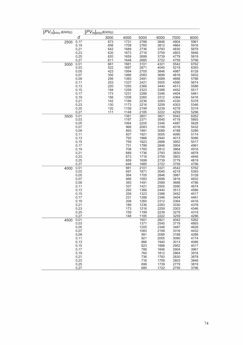
74

[PVIS]kWp (€/kWp) [PVIN]kWp(€/kWp) d 3000 4000 5000 6000 7000 8000

2500 0,17 673 1731 2788 3846 4904 5961 0,19 656 1708 2760 3812 4864 5916 0,21 642 1689 2736 3783 4830 5878 0,23 630 1673 2716 3759 4803 5846 0,25 620 1659 2699 3739 4779 5819 0,27 611 1648 2685 3722 4759 5796

3000 0,01 661 1881 3101 4321 5542 6762 0,03 522 1697 2871 4045 5219 6393 0,05 423 1564 2705 3846 4987 6128 0,07 350 1466 2583 3699 4816 5932 0,09 295 1393 2491 3589 4688 5786 0,11 253 1337 2421 3505 4590 5674 0,13 220 1293 2366 3440 4513 5586 0,15 194 1259 2323 3388 4452 5517 0,17 173 1231 2288 3346 4404 5461 0,19 156 1208 2260 3312 4364 5416 0,21 142 1189 2236 3283 4330 5378 0,23 130 1173 2216 3259 4303 5346 0,25 120 1159 2199 3239 4279 5319 0,27 111 1148 2185 3222 4259 5296

3500 0,01 1381 2601 3821 5042 6262 0,03 1197 2371 3545 4719 5893 0,05 1064 2205 3346 4487 5628 0,07 966 2083 3199 4316 5432 0,09 893 1991 3089 4188 5286 0,11 837 1921 3005 4090 5174 0,13 793 1866 2940 4013 5086 0,15 759 1823 2888 3952 5017 0,17 731 1788 2846 3904 4961 0,19 708 1760 2812 3864 4916 0,21 689 1736 2783 3830 4878 0,23 673 1716 2759 3803 4846 0,25 659 1699 2739 3779 4819 0,27 648 1685 2722 3759 4796

4000 0,01 881 2101 3321 4542 5762 0,03 697 1871 3045 4219 5393 0,05 564 1705 2846 3987 5128 0,07 466 1583 2699 3816 4932 0,09 393 1491 2589 3688 4786 0,11 337 1421 2505 3590 4674 0,13 293 1366 2440 3513 4586 0,15 259 1323 2388 3452 4517 0,17 231 1288 2346 3404 4461 0,19 208 1260 2312 3364 4416 0,21 189 1236 2283 3330 4378 0,23 173 1216 2259 3303 4346 0,25 159 1199 2239 3279 4319 0,27 148 1185 2222 3259 4296

4500 0,01 1601 2821 4042 5262 0,03 1371 2545 3719 4893 0,05 1205 2346 3487 4628 0,07 1083 2199 3316 4432 0,09 991 2089 3188 4286 0,11 921 2005 3090 4174 0,13 866 1940 3013 4086 0,15 823 1888 2952 4017 0,17 788 1846 2904 3961 0,19 760 1812 2864 3916 0,21 736 1783 2830 3878 0,23 716 1759 2803 3846 0,25 699 1739 2779 3819 0,27 685 1722 2759 3796

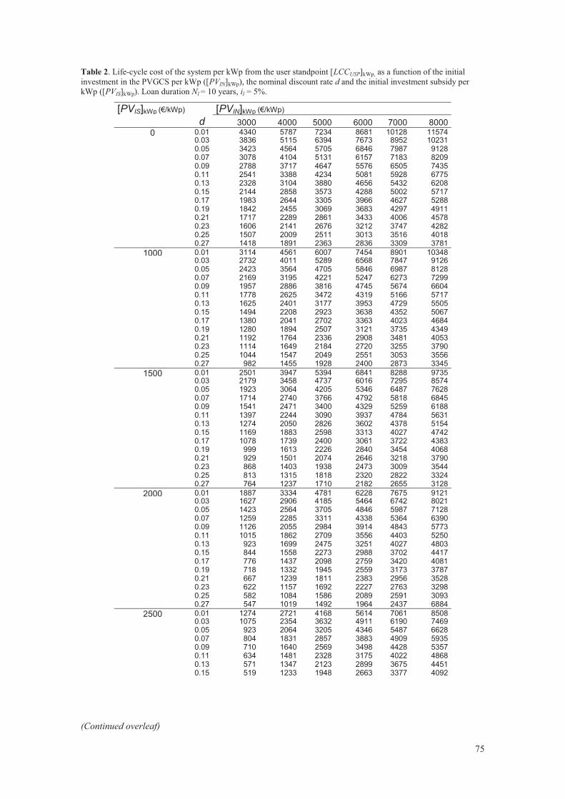
75

Table 2. Life-cycle cost of the system per kWp from the user standpoint [LCCUSP]kWp, as a function of the initial investment in the PVGCS per kWp ([PVIN]kWp), the nominal discount rate d and the initial investment subsidy per kWp ([PVIS]kWp). Loan duration Nl = 10 years, il = 5%.

[PVIS]kWp (€/kWp) [PVIN]kWp (€/kWp) d 3000 4000 5000 6000 7000 8000

0 0.01 4340 5787 7234 8681 10128 11574 0.03 3836 5115 6394 7673 8952 10231 0.05 3423 4564 5705 6846 7987 9128 0.07 3078 4104 5131 6157 7183 8209 0.09 2788 3717 4647 5576 6505 7435 0.11 2541 3388 4234 5081 5928 6775 0.13 2328 3104 3880 4656 5432 6208 0.15 2144 2858 3573 4288 5002 5717 0.17 1983 2644 3305 3966 4627 5288 0.19 1842 2455 3069 3683 4297 4911 0.21 1717 2289 2861 3433 4006 4578 0.23 1606 2141 2676 3212 3747 4282 0.25 1507 2009 2511 3013 3516 4018 0.27 1418 1891 2363 2836 3309 3781

1000 0.01 3114 4561 6007 7454 8901 10348 0.03 2732 4011 5289 6568 7847 9126 0.05 2423 3564 4705 5846 6987 8128 0.07 2169 3195 4221 5247 6273 7299 0.09 1957 2886 3816 4745 5674 6604 0.11 1778 2625 3472 4319 5166 5717 0.13 1625 2401 3177 3953 4729 5505 0.15 1494 2208 2923 3638 4352 5067 0.17 1380 2041 2702 3363 4023 4684 0.19 1280 1894 2507 3121 3735 4349 0.21 1192 1764 2336 2908 3481 4053 0.23 1114 1649 2184 2720 3255 3790 0.25 1044 1547 2049 2551 3053 3556 0.27 982 1455 1928 2400 2873 3345

1500 0.01 2501 3947 5394 6841 8288 9735 0.03 2179 3458 4737 6016 7295 8574 0.05 1923 3064 4205 5346 6487 7628 0.07 1714 2740 3766 4792 5818 6845 0.09 1541 2471 3400 4329 5259 6188 0.11 1397 2244 3090 3937 4784 5631 0.13 1274 2050 2826 3602 4378 5154 0.15 1169 1883 2598 3313 4027 4742 0.17 1078 1739 2400 3061 3722 4383 0.19 999 1613 2226 2840 3454 4068 0.21 929 1501 2074 2646 3218 3790 0.23 868 1403 1938 2473 3009 3544 0.25 813 1315 1818 2320 2822 3324 0.27 764 1237 1710 2182 2655 3128

2000 0.01 1887 3334 4781 6228 7675 9121 0.03 1627 2906 4185 5464 6742 8021 0.05 1423 2564 3705 4846 5987 7128 0.07 1259 2285 3311 4338 5364 6390 0.09 1126 2055 2984 3914 4843 5773 0.11 1015 1862 2709 3556 4403 5250 0.13 923 1699 2475 3251 4027 4803 0.15 844 1558 2273 2988 3702 4417 0.17 776 1437 2098 2759 3420 4081 0.19 718 1332 1945 2559 3173 3787 0.21 667 1239 1811 2383 2956 3528 0.23 622 1157 1692 2227 2763 3298 0.25 582 1084 1586 2089 2591 3093 0.27 547 1019 1492 1964 2437 6884

2500 0.01 1274 2721 4168 5614 7061 8508 0.03 1075 2354 3632 4911 6190 7469 0.05 923 2064 3205 4346 5487 6628 0.07 804 1831 2857 3883 4909 5935 0.09 710 1640 2569 3498 4428 5357 0.11 634 1481 2328 3175 4022 4868 0.13 571 1347 2123 2899 3675 4451 0.15 519 1233 1948 2663 3377 4092

(Continued overleaf)

76

[PVIS]kWp(€/kWp) [PVIN]kWp (€/kWp) d 3000 4000 5000 6000 7000 8000

2500 0.17 475 1136 1797 2458 3119 3780 0.19 437 1051 1665 2278 2892 3506 0.21 404 976 1549 2121 2693 3265 0.23 376 911 1446 1981 2517 3052 0.25 351 853 1355 1857 2360 2862 0.27 329 801 1274 1747 2219 2692

3000 0.01 661 2108 3554 5001 6448 7895 0.03 522 1801 3080 4359 5638 6917 0.05 423 1564 2705 3846 4987 6128 0.07 350 1376 2402 3428 4454 5480 0.09 295 1224 2153 3083 4012 4941 0.11 253 1100 1946 2793 3640 4487 0.13 220 996 1772 2548 3324 4100 0.15 194 909 1623 2338 3052 3767 0.17 173 834 1495 2156 2817 3478 0.19 156 770 1384 1997 2611 3225 0.21 142 714 1286 1858 2431 3003 0.23 130 665 1200 1735 2271 2806 0.25 120 622 1124 1626 2129 2631 0.27 111 583 1056 1529 2001 2474

3500 0.01 1494 2941 4388 5835 7281 0.03 1249 2528 3807 5085 6364 0.05 1064 2205 3346 4487 5628 0.07 921 1947 2973 3999 5025 0.09 808 1738 2667 3596 4526 0.11 718 1565 2412 3259 4106 0.13 645 1421 2197 2973 3749 0.15 584 1298 2013 2727 3442 0.17 532 1193 1854 2515 3176 0.19 489 1103 1716 2330 2944 0.21 451 1024 1596 2168 2740 0.23 419 954 1489 2025 2560 0.25 391 893 1395 1897 2400 0.27 366 838 1311 1784 2256

4000 0.01 881 2328 3775 5221 6668 0.03 697 1975 3254 4533 5812 0.05 564 1705 2846 3987 5128 0.07 466 1492 2518 3545 4571 0.09 393 1322 2252 3181 4110 0.11 337 1184 2031 2878 3724 0.13 293 1069 1845 2621 3397 0.15 259 973 1688 2402 3117 0.17 231 892 1553 2214 2875 0.19 208 822 1436 2049 2663 0.21 189 761 1333 1906 2478 0.23 173 708 1243 1779 2314 0.25 159 662 1164 1666 2168 0.27 148 620 1093 1566 2038

4500 0.01 1714 3161 4608 6055 0.03 1423 2702 3981 5260 0.05 1205 2346 3487 4628 0.07 1037 2064 3090 4116 0.09 907 1836 2765 3695 0.11 802 1649 2496 3343 0.13 718 1494 2270 3046 0.15 648 1363 2077 2792 0.17 590 1251 1912 2573 0.19 541 1155 1768 2382 0.21 499 1071 1643 2215 0.23 462 997 1533 2068 0.25 430 933 1435 1937 0.27 403 875 1348 1821

77

Table 3. Life-cycle cost of the system per kWp from the user standpoint [LCCUSP]kWp, as a function of the initial investment in the PVGCS per kWp ([PVIN]kWp), the nominal discount rate d and the initial investment subsidy per kWp ([PVIS]kWp). Loan duration Nl = 20 years, il = 5%.

[PVIS]kWp(€/kWp) [PVIN]kWp (€/kWp) d 3000 4000 5000 6000 7000 8000

0 0.01 5005 6673 8341 10010 11678 13346 0.03 4104 5472 6840 8208 9576 10944 0.05 3423 4564 5705 6846 7987 9128 0.07 2900 3867 4833 5800 6766 7733 0.09 2492 3323 4154 4984 5815 6646 0.11 2170 2893 3616 4339 5063 5786 0.13 1911 2548 3185 3822 4459 5096 0.15 1701 2268 2835 3401 3968 4535 0.17 1528 2037 2546 3055 3565 4074 0.19 1384 1845 2306 2768 3229 3690 0.21 1263 1684 2104 2525 2946 3367 0.23 1160 1546 1933 2319 2706 3092 0.25 1071 1428 1786 2143 2500 2857 0.27 995 1327 1658 1990 2322 2653

1000 0.01 3557 5225 6893 8561 10230 11898 0.03 2910 4278 5646 7014 8382 9750 0.05 2423 3564 4705 5846 6987 8128 0.07 2050 3016 3983 4950 5916 6883 0.09 1760 2590 3421 4252 5083 5913 0.11 1531 2254 2977 3700 4424 4535 0.13 1347 1984 2621 3258 3895 4532 0.15 1198 1765 2332 2899 3466 4033 0.17 1076 1585 2095 2604 3113 3622 0.19 974 1436 1897 2358 2819 3281 0.21 889 1310 1731 2152 2572 2993 0.23 816 1203 1589 1976 2363 2749 0.25 754 1111 1468 1825 2183 2540 0.27 700 1032 1364 1695 2027 2358

1500 0.01 2833 4501 6169 7837 9506 11174 0.03 2313 3681 5049 6417 7785 9153 0.05 1923 3064 4205 5346 6487 7628 0.07 1625 2591 3558 4525 5491 6458 0.09 1393 2224 3055 3886 4716 5547 0.11 1211 1934 2658 3381 4104 4827 0.13 1065 1702 2339 2976 3613 4250 0.15 947 1514 2081 2648 3215 3782 0.17 850 1360 1869 2378 2887 3397 0.19 770 1231 1692 2154 2615 3076 0.21 702 1123 1544 1965 2386 2807 0.23 645 1031 1418 1804 2191 2577 0.25 595 953 1310 1667 2024 2381 0.27 553 885 1216 1548 1879 2211

2000 0.01 2109 3777 5445 7113 8782 10450 0.03 1716 3084 4452 5820 7188 8556 0.05 1423 2564 3705 4846 5987 7128 0.07 1200 2166 3133 4100 5066 6033 0.09 1027 1858 2689 3519 4350 5181 0.11 892 1615 2338 3061 3785 4508 0.13 784 1421 2058 2695 3332 3969 0.15 696 1263 1830 2397 2964 3531 0.17 625 1134 1643 2152 2662 3171 0.19 565 1026 1488 1949 2410 2871 0.21 515 936 1357 1778 2199 2620 0.23 473 860 1246 1633 2019 2406 0.25 437 794 1151 1508 1865 2222 0.27 406 737 1069 1400 1732 5555

2500 0.01 1385 3053 4721 6389 8058 9726 0.03 1119 2487 3855 5223 6591 7959 0.05 923 2064 3205 4346 5487 6628 0.07 775 1741 2708 3675 4641 5608 0.09 661 1492 2322 3153 3984 4815 0.11 572 1295 2019 2742 3465 4188 0.13 502 1139 1776 2413 3050 3687 0.15 445 1012 1579 2146 2713 3280

(Continued overleaf)

78

[PVIS]kWp(€/kWp) [PVIN]kWp (€/kWp) d 3000 4000 5000 6000 7000 8000

2500 0.17 399 908 1417 1927 2436 2945 0.19 361 822 1283 1744 2206 2667 0.21 328 749 1170 1591 2012 2433 0.23 301 688 1074 1461 1848 2234 0.25 278 635 992 1350 1707 2064 0.27 258 590 921 1253 1585 1916

3000 0.01 661 2329 3997 5665 7334 9002 0.03 522 1890 3258 4626 5994 7362 0.05 423 1564 2705 3846 4987 6128 0.07 350 1316 2283 3249 4216 5183 0.09 295 1125 1956 2787 3618 4448 0.11 253 976 1699 2422 3146 3869 0.13 220 857 1494 2131 2768 3405 0.15 194 761 1328 1895 2462 3028 0.17 173 682 1191 1701 2210 2719 0.19 156 617 1078 1540 2001 2462 0.21 142 563 983 1404 1825 2246 0.23 130 516 903 1289 1676 2062 0.25 120 477 834 1191 1548 1905 0.27 111 442 774 1106 1437 1769

3500 0.01 1605 3273 4941 6610 8278 0.03 1293 2661 4029 5397 6765 0.05 1064 2205 3346 4487 5628 0.07 891 1858 2824 3791 4758 0.09 759 1590 2421 3251 4082 0.11 656 1380 2103 2826 3549 0.13 575 1212 1849 2486 3123 0.15 510 1077 1644 2210 2777 0.17 456 966 1475 1984 2493 0.19 412 874 1335 1796 2257 0.21 376 797 1217 1638 2059 0.23 345 731 1118 1504 1891 0.25 318 675 1032 1389 1747 0.27 295 627 958 1290 1622

4000 0.01 881 2549 4217 5886 7554 0.03 697 2064 3432 4800 6168 0.05 564 1705 2846 3987 5128 0.07 466 1433 2399 3366 4333 0.09 393 1224 2054 2885 3716 0.11 337 1060 1783 2507 3230 0.13 293 930 1567 2204 2841 0.15 259 825 1392 1959 2526 0.17 231 740 1249 1758 2268 0.19 208 669 1130 1592 2053 0.21 189 610 1031 1451 1872 0.23 173 559 946 1333 1719 0.25 159 517 874 1231 1588 0.27 148 479 811 1143 1474

4500 0.01 1825 3493 5162 6830 0.03 1468 2835 4203 5571 0.05 1205 2346 3487 4628 0.07 1008 1974 2941 3908 0.09 857 1688 2519 3350 0.11 741 1464 2187 2910 0.13 648 1285 1922 2559 0.15 574 1141 1708 2275 0.17 514 1023 1533 2042 0.19 464 926 1387 1848 0.21 423 844 1265 1686 0.23 388 774 1161 1548 0.25 358 715 1072 1429 0.27 332 664 995 1327

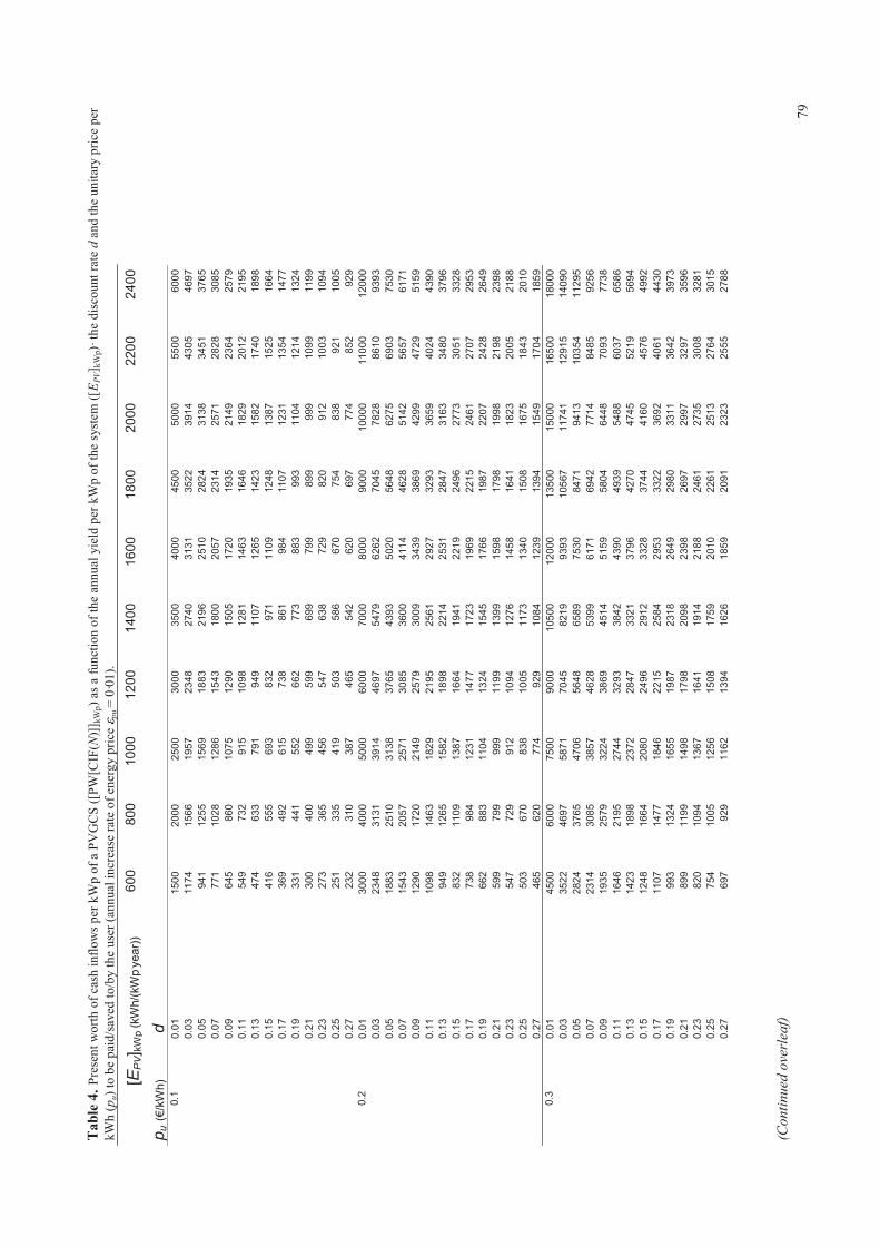
79

Tab

le 4

. Pre

sent

wor

th o

f cas

h in

flow

s per

kW

p of

a P

VG

CS

([PW

[CIF

(N)]]

kWp)

as a

func

tion

of th

e an

nual

yie

ld p

er k

Wp

of th

e sy

stem

([E P

V]kW

p)· t

he d

isco

unt r

ate

d an

d th

e un

itary

pric

e pe

r kW

h (p

u) to

be

paid

/sav

ed to

/by

the

user

(ann

ual i

ncre

ase

rate

of e

nerg

y pr

ice

pu =

0·0

1).

[EP

V]kW

p (k

Wh/

(kW

p. year

))

600

800

1000

12

00

1400

16

00

1800

20

00

2200

24

00

p u (€/kWh)

d

0.1

0.01

1500

20

00

2500

30

00

3500

40

00

4500

50

00

5500

60

00

0.03

1174

15

66

1957

23

48

2740

31

31

3522

39

14

4305

46

97

0.

05

94

1

1255

15

69

1883

21

96

2510

28

24

3138

34

51

3765

0.07

771

10

28

1286

15

43

1800

20

57

2314

25

71

2828

30

85

0.

09

64

5

860

10

75

1290

15

05

1720

19

35

2149

23

64

2579

0.11

549

73

2

915

10

98

1281

14

63

1646

18

29

2012

21

95

0.

13

47

4

633

79

1

949

11

07

1265

14

23

1582

17

40

1898

0.15

416

55

5

693

83

2

971

11

09

1248

13

87

1525

16

64

0.

17

36

9

492

61

5

738

86

1

984

11

07

1231

13

54

1477

0.19

331

44

1

552

66

2

773

88

3

993

11

04

1214

13

24

0.

21

30

0

400

49

9

599

69

9

799

89

9

999

10

99

1199

0.23

273

36

5

456

54

7

638

72

9

820

91

2

1003

10

94

0.

25

25

1

335

41

9

503

58

6

670

75

4

838

92

1

1005

0.27

232

31

0

387

46

5

542

62

0

697

77

4

852

92

9

0.2

0.01

3000

40

00

5000

60

00

7000

80

00

9000

10

000

11

000

12

000

0.

03

23

48

3131

39

14

4697

54

79

6262

70

45

7828

86

10

9393

0.05

1883

25

10

3138

37

65

4393

50

20

5648

62

75

6903

75

30

0.

07

15

43

2057

25

71

3085

36

00

4114

46

28

5142

56

57

6171

0.09

1290

17

20

2149

25

79

3009

34

39

3869

42

99

4729

51

59

0.

11

10

98

1463

18

29

2195

25

61

2927

32

93

3659

40

24

4390

0.13

949

12

65

1582

18

98

2214

25

31

2847

31

63

3480

37

96

0.

15

83

2

1109

13

87

1664

19

41

2219

24

96

2773

30

51

3328

0.17

738

98

4

1231

14

77

1723

19

69

2215

24

61

2707

29

53

0.

19

66

2

883

11

04

1324

15

45

1766

19

87

2207

24

28

2649

0.21

599

79

9

999

11

99

1399

15

98

1798

19

98

2198

23

98

0.

23

54

7

729

91

2

1094

12

76

1458

16

41

1823

20

05

2188

0.25

503

67

0

838

10

05

1173

13

40

1508

16

75

1843

20

10

0.

27

46

5

620

77

4

929

10

84

1239

13

94

1549

17

04

1859

0.

3 0.

01

45

00

6000

75

00

9000

10

500

12

000

13

500

15

000

16

500

18

000

0.

03

35

22

4697

58

71

7045

82

19

9393

10

567

11

741

12

915

14

090

0.05

2824

37

65

4706

56

48

6589

75

30

8471

94

13

1035

4

1129

5

0.

07

23

14

3085

38

57

4628

53

99

6171

69

42

7714

84

85

9256

0.09

1935

25

79

3224

38

69

4514

51

59

5804

64

48

7093

77

38

0.

11

16

46

2195

27

44

3293

38

42

4390

49

39

5488

60

37

6586

0.13

1423

18

98

2372

28

47

3321

37

96

4270

47

45

5219

56

94

0.

15

12

48

1664

20

80

2496

29

12

3328

37

44

4160

45

76

4992

0.17

1107

14

77

1846

22

15

2584

29

53

3322

36

92

4061

44

30

0.

19

99

3

1324

16

55

1987

23

18

2649

29

80

3311

36

42

3973

0.21

899

11

99

1498

17

98

2098

23

98

2697

29

97

3297

35

96

0.

23

82

0

1094

13

67

1641

19

14

2188

24

61

2735

30

08

3281

0.25

754

10

05

1256

15

08

1759

20

10

2261

25

13

2764

30

15

0.

27

69

7

929

11

62

1394

16

26

1859

20

91

2323

25

55

2788

(C

ontin

ued

over

leaf

)

80

[EP

V] kW

p (k

Wh/

(kW

p. year

)) 60

0 80

0 10

00

1200

14

00

1600

18

00

2000

22

00

2400

p u (€/kWh)

d

0.4

0.01

6000

80

00

1000

0

1200

0

1400

0

1600

0

1800

0

2000

0

2200

0

2400

0

0.03

4697

62

62

7828

93

93

1095

9

1252

4

1409

0

1565

5

1722

1

1878

6

0.

05

37

65

5020

62

75

7530

87

85

1004

0

1129

5

1255

0

1380

5

1506

0

0.

07

30

85

4114

51

42

6171

71

99

8228

92

56

1028

5

1131

3

1234

2

0.

09

25

79

3439

42

99

5159

60

19

6878

77

38

8598

94

58

1031

8

0.

11

21

95

2927

36

59

4390

51

22

5854

65

86

7317

80

49

8781

0.13

1898

25

31

3163

37

96

4429

50

61

5694

63

27

6959

75

92

0.

15

16

64

2219

27

73

3328

38

83

4437

49

92

5547

61

01

6656

0.17

1477

19

69

2461

29

53

3446

39

38

4430

49

22

5414

59

07

0.

19

13

24

1766

22

07

2649

30

90

3532

39

73

4415

48

56

5297

0.21

1199

15

98

1998

23

98

2797

31

97

3596

39

96

4395

47

95

0.

23

10

94

1458

18

23

2188

25

52

2917

32

81

3646

40

11

4375

0.25

1005

13

40

1675

20

10

2345

26

80

3015

33

50

3685

40

20

0.

27

92

9

1239

15

49

1859

21

68

2478

27

88

3098

34

07

3717

0.

5 0.

01

75

00

1000

0

1250

0

1500

0

1750

0

2000

0

2250

0

2500

0

2750

0

3000

0

0.03

5871

78

28

9784

11

741

13

698

15

655

17

612

19

569

21

526

23

483

0.05

4706

62

75

7844

94

13

1098

1

1255

0

1411

9

1568

8

1725

6

1882

5

0.

07

38

57

5142

64

28

7714

89

99

1028

5

1157

0

1285

6

1414

1

1542

7

0.

09

32

24

4299

53

74

6448

75

23

8598

96

73

1074

7

1182

2

1289

7

0.

11

27

44

3659

45

73

5488

64

03

7317

82

32

9147

10

061

10

976

0.13

2372

31

63

3954

47

45

5536

63

27

7117

79

08

8699

94

90

0.

15

20

80

2773

34

67

4160

48

53

5547

62

40

6933

76

27

8320

0.17

1846

24

61

3076

36

92

4307

49

22

5537

61

53

6768

73

83

0.

19

16

55

2207

27

59

3311

38

63

4415

49

66

5518

60

70

6622

0.21

1498

19

98

2497

29

97

3496

39

96

4495

49

95

5494

59

94

0.

23

13

67

1823

22

79

2735

31

90

3646

41

02

4558

50

13

5469

0.25

1256

16

75

2094

25

13

2932

33

50

3769

41

88

4607

50

26

0.

27

11

62

1549

19

36

2323

27

10

3098

34

85

3872

42

59

4646

0.

6 0.

01

90

00

1200

0

1500

0

1800

0

2100

0

2400

0

2700

0

3000

0

3300

0

3600

0

0.03

7045

93

93

1174

1

1409

0

1643

8

1878

6

2113

4

2348

3

2583

1

2817

9

0.

05

56

48

7530

94

13

1129

5

1317

8

1506

0

1694

3

1882

5

2070

8

2259

0

0.

07

46

28

6171

77

14

9256

10

799

12

342

13

884

15

427

16

970

18

512

0.09

3869

51

59

6448

77

38

9028

10

318

11

607

12

897

14

187

15

476

0.11

3293

43

90

5488

65

86

7683

87

81

9878

10

976

12

073

13

171

0.13

2847

37

96

4745

56

94

6643

75

92

8541

94

90

1043

9

1138

8

0.

15

24

96

3328

41

60

4992

58

24

6656

74

88

8320

91

52

9984

0.17

2215

29

53

3692

44

30

5168

59

07

6645

73

83

8122

88

60

0.

19

19

87

2649

33

11

3973

46

35

5297

59

60

6622

72

84

7946

0.21

1798

23

98

2997

35

96

4196

47

95

5394

59

94

6593

71

93

0.

23

16

41

2188

27

35

3281

38

28

4375

49

22

5469

60

16

6563

0.25

1508

20

10

2513

30

15

3518

40

20

4523

50

26

5528

60

31

0.

27

13

94

1859

23

23

2788

32

52

3717

41

82

4646

51

11

5576

81

Tab

le 5

. Pre

sent

wor

th o

f cas

h in

flow

s per

kW

p of

a P

VG

CS

([PW

[CIF

(N)]]

kWp)

as a

func

tion

of th

e an

nual

yie

ld p

er k

Wp

of th

e sy

stem

([E P

V]kW

p)· t

he d

isco

unt r

ate

d an

d th

e un

itary

pric

e pe

r kW

h (p

u) to

be

paid

/sav

ed to

/by

the

user

(ann

ual i

ncre

ase

rate

of e

nerg

y pr

ice

p pu =

0·0

2).

[EP

V] kW

p (k

Wh/

(kW

p. year

)) 60

0 80

0 10

00

1200

14

00

1600

18

00

2000

22

00

2400

p u (€/kWh)

d

0.1

0.01

1709

22

79

2849

34

19

3988

45

58

5128

56

98

6267

68

37

0.03

1325

17

66

2208

26

49

3091

35

32

3974

44

15

4857

52

98

0.

05

10

52

1402

17

53

2103

24

54

2804

31

55

3506

38

56

4207

0.07

854

11

39

1423

17

08

1993

22

77

2562

28

47

3131

34

16

0.

09

70

8

944

11

80

1416

16

52

1888

21

24

2360

25

96

2832

0.11

598

79

7

996

11

96

1395

15

94

1794

19

93

2192

23

92

0.

13

51

3

684

85

6

1027

11

98

1369

15

40

1711

18

82

2053

0.15

447

59

6

746

89

5

1044

11

93

1342

14

91

1640

17

89

0.

17

39

5

526

65

8

790

92

1

1053

11

84

1316

14

48

1579

0.19

352

47

0

587

70

5

822

94

0

1057

11

75

1292

14

09

0.

21

31

8

423

52

9

635

74

1

847

95

3

1059

11

65

1270

0.23

289

38

5

481

57

7

674

77

0

866

96

2

1059

11

55

0.

25

26

4

353

44

1

529

61

7

705

79

3

881

97

0

1058

0.27

244

32

5

406

48

8

569

65

0

731

81

3

894

97

5

0.2

0.01

3419

45

58

5698

68

37

7977

91

16

1025

6

1139

5

1253

5

1367

4

0.03

2649

35

32

4415

52

98

6181

70

65

7948

88

31

9714

10

597

0.05

2103

28

04

3506

42

07

4908

56

09

6310

70

11

7712

84

13

0.

07

17

08

2277

28

47

3416

39

85

4555

51

24

5693

62

63

6832

0.09

1416

18

88

2360

28

32

3304

37

76

4248

47

20

5192

56

64

0.

11

11

96

1594

19

93

2392

27

90

3189

35

87

3986

43

84

4783

0.13

1027

13

69

1711

20

53

2396

27

38

3080

34

22

3765

41

07

0.

15

89

5

1193

14

91

1789

20

87

2386

26

84

2982

32

80

3578

0.17

790

10

53

1316

15

79

1842

21

06

2369

26

32

2895

31

58

0.

19

70

5

940

11

75

1409

16

44

1879

21

14

2349

25

84

2819

0.21

635

84

7

1059

12

70

1482

16

94

1906

21

17

2329

25

41

0.

23

57

7

770

96

2

1155

13

47

1540

17

32

1925

21

17

2310

0.25

529

70

5

881

10

58

1234

14

10

1587

17

63

1939

21

16

0.

27

48

8

650

81

3

975

11

38

1300

14

63

1625

17

88

1950

0.

3 0.

01

51

28

6837

85

46

1025

6

1196

5

1367

4

1538

3

1709

3

1880

2

2051

1

0.03

3974

52

98

6623

79

48

9272

10

597

11

921

13

246

14

571

15

895

0.05

3155

42

07

5258

63

10

7362

84

13

9465

10

517

11

568

12

620

0.07

2562

34

16

4270

51

24

5978

68

32

7686

85

40

9394

10

248

0.09

2124

28

32

3540

42

48

4956

56

64

6372

70

79

7787

84

95

0.

11

17

94

2392

29

89

3587

41

85

4783

53

81

5979

65

77

7175

0.13

1540

20

53

2567

30

80

3594

41

07

4620

51

34

5647

61

60

0.

15

13

42

1789

22

37

2684

31

31

3578

40

26

4473

49

20

5368

0.17

1184

15

79

1974

23

69

2764

31

58

3553

39

48

4343

47

37

0.

19

10

57

1409

17

62

2114

24

67

2819

31

71

3524

38

76

4228

0.21

953

12

70

1588

19

06

2223

25

41

2858

31

76

3494

38

11

0.

23

86

6

1155

14

44

1732

20

21

2310

25

99

2887

31

76

3465

0.25

793

10

58

1322

15

87

1851

21

16

2380

26

44

2909

31

73

0.

27

73

1

975

12

19

1463

17

06

1950

21

94

2438

26

82

2925

(C

ontin

ued

over

leaf

)

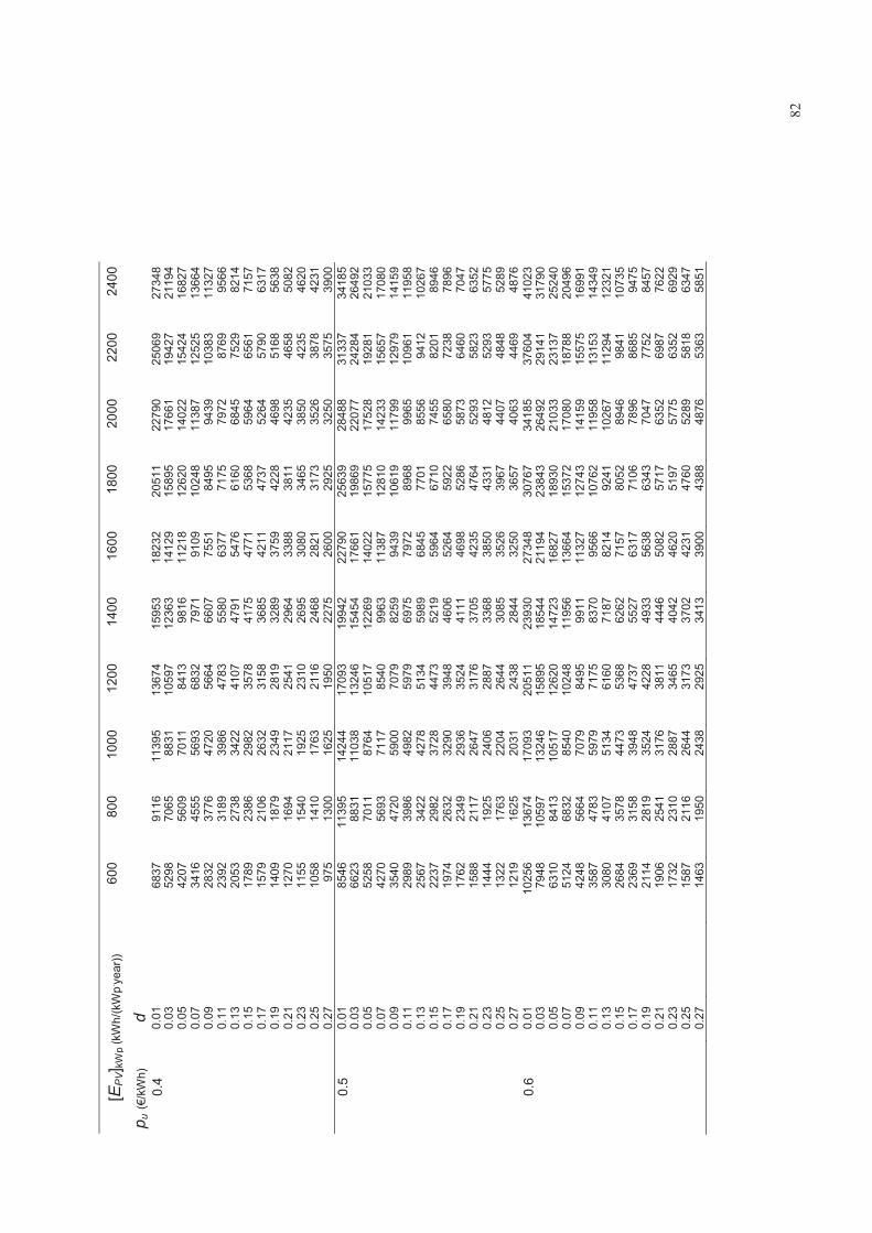
82

[EP

V] kW

p (k

Wh/

(kW

p. year

)) 60

0 80

0 10

00

1200

14

00

1600

18

00

2000

22

00

2400

p u (€/kWh)

d

0.4

0.01

6837

91

16

1139

5

1367

4

1595

3

1823

2

2051

1

2279

0

2506

9

2734

8

0.03

5298

70

65

8831

10

597

12

363

14

129

15

895

17

661

19

427

21

194

0.05

4207

56

09

7011

84

13

9816

11

218

12

620

14

022

15

424

16

827

0.07

3416

45

55

5693

68

32

7971

91

09

1024

8

1138

7

1252

5

1366

4

0.

09

28

32

3776

47

20

5664

66

07

7551

84

95

9439

10

383

11

327

0.11

2392

31

89

3986

47

83

5580

63

77

7175

79

72

8769

95

66

0.

13

20

53

2738

34

22

4107

47

91

5476

61

60

6845

75

29

8214

0.15

1789

23

86

2982

35

78

4175

47

71

5368

59

64

6561

71

57

0.

17

15

79

2106

26

32

3158

36

85

4211

47

37

5264

57

90

6317

0.19

1409

18

79

2349

28

19

3289

37

59

4228

46

98

5168

56

38

0.

21

12

70

1694

21

17

2541

29

64

3388

38

11

4235

46

58

5082

0.23

1155

15

40

1925

23

10

2695

30

80

3465

38

50

4235

46

20

0.

25

10

58

1410

17

63

2116

24

68

2821

31

73

3526

38

78

4231

0.27

975

13

00

1625

19

50

2275

26

00

2925

32

50

3575

39

00

0.5

0.01

8546

11

395

14

244

17

093

19

942

22

790

25

639

28

488

31

337

34

185

0.

03

66

23

8831

11

038

13

246

15

454

17

661

19

869

22

077

24

284

26

492

0.05

5258

70

11

8764

10

517

12

269

14

022

15

775

17

528

19

281

21

033

0.07

4270

56

93

7117

85

40

9963

11

387

12

810

14

233

15

657

17

080

0.09

3540

47

20

5900

70

79

8259

94

39

1061

9

1179

9

1297

9

1415

9

0.

11

29

89

3986

49

82

5979

69

75

7972

89

68

9965

10

961

11

958

0.13

2567

34

22

4278

51

34

5989

68

45

7701

85

56

9412

10

267

0.15

2237

29

82

3728

44

73

5219

59

64

6710

74

55

8201

89

46

0.

17

19

74

2632

32

90

3948

46

06

5264

59

22

6580

72

38

7896

0.19

1762

23

49

2936

35

24

4111

46

98

5286

58

73

6460

70

47

0.

21

15

88

2117

26

47

3176

37

05

4235

47

64

5293

58

23

6352

0.23

1444

19

25

2406

28

87

3368

38

50

4331

48

12

5293

57

75

0.

25

13

22

1763

22

04

2644

30

85

3526

39

67

4407

48

48

5289

0.27

1219

16

25

2031

24

38

2844

32

50

3657

40

63

4469

48

76

0.6

0.01

1025

6

1367

4

1709

3

2051

1

2393

0

2734

8

3076

7

3418

5

3760

4

4102

3

0.03

7948

10

597

13

246

15

895

18

544

21

194

23

843

26

492

29

141

31

790

0.05

6310

84

13

1051

7

1262

0

1472

3

1682

7

1893

0

2103

3

2313

7

2524

0

0.

07

51

24

6832

85

40

1024

8

1195

6

1366

4

1537

2

1708

0

1878

8

2049

6

0.

09

42

48

5664

70

79

8495

99

11

1132

7

1274

3

1415

9

1557

5

1699

1

0.

11

35

87

4783

59

79

7175

83

70

9566

10

762

11

958

13

153

14

349

0.13

3080

41

07

5134

61

60

7187

82

14

9241

10

267

11

294

12

321

0.15

2684

35

78

4473

53

68

6262

71

57

8052

89

46

9841

10

735

0.17

2369

31

58

3948

47

37

5527

63

17

7106

78

96

8685

94

75

0.

19

21

14

2819

35

24

4228

49

33

5638

63

43

7047

77

52

8457

0.21

1906

25

41

3176

38

11

4446

50

82

5717

63

52

6987

76

22

0.

23

17

32

2310

28

87

3465

40

42

4620

51

97

5775

63

52

6929

0.25

1587

21

16

2644

31

73

3702

42

31

4760

52

89

5818

63

47

0.

27

14

63

1950

24

38

2925

34

13

3900

43

88

4876

53

63

5851

83

APPENDIX II OF SECTION 5: TERMINOLOGY

[EPV]kWp Normalised (per kWp) annual PV electricity yield (kWh·kWp-1·yr-1).

[LCCUSP]kWp Normalised (per kWp) life – cycle cost of the PVGCS from the user standpoint (€·kWp-1).

[PVIS ]kWp Normalised (per kWp) initial buy-down or subsidy (€·kWp-1).

[PVIN]kWp Normalised (per kWp) initial investment on the PVGCS (€·kWp-1). [PW[CIF(N)]]kWp Normalised (per kWp) present worth of the cash inflows from a PVGCS through its

useful life (€·kWp-1).

d Nominal discount rate.

EPV Annual PV electricity yield (kWh).

il Annual loan interest.

g Annual inflation rate.

IRR Internal rate of return.

LCCUSP Life - cycle cost of the PVGCS from the user standpoint (€).

N Useful life of the PVGCS (years).

Nl Time duration of loan (years).

NPV Net present value (€).

pu PV-electricity unitary price paid/saved to/by the user (€·kWh-1)

PVIS Initial buy-down or subsidy (€).

PVIN Initial investment on the PVGCS (€). PW[CIF(N)] Present worth of the cash inflows from a PVGCS through its useful life (€).

pu Annual increase rate of the energy price consumed/sold from/to the grid

APPENDIX: MAIN TECHNICAL AND CONTRACTUAL POINTS TO BE CHECKED AND COMPARED WHEN EXAMINING A PROPOSAL FROM AN EPC SUPPLIER This appendix is aimed at verifying through cross-checks if the EPC (engineering, procurement and construction) supplier proposal is sound. It must be borne in mind the high important of this hot issue. Making sure that a proposal guarantees a minimum production, a long-lasting durability and reliability is the key to avoid misunderstandings and future litigations. Some examples of these cross-checks are provided below:

Is the EPC supplier experienced and skilled? Unskilled PVPPs EPC suppliers are not infrequent, unfortunately

84

Is a minimum electricity production per kWp guaranteed? Is this production

clearly linked to an easily measurable parameter (e.g.: irradiation measured by an external and independent body)? Avoid production warranties related to performance indices which are difficult and not straightforward to understand and measure (e.g.: performance ratio)

Are protective measures suitably sized and planned in the proposal? Fuses,

voltage surge arrestors, good metal works earthening, etc. sometimes are omitted or wrongly sized

Is the operation and maintenance contract (O&M, usually offered by the EPC

supplier) clear and rigorous?

Does the contract include a reliable insurance (min.100% insurance coverage:

theft, natural disasters, vandalism, etc.)?

Is the EPC supplier willing to let the PVPP undergo a quality check (careful

visual inspection, measuring the actual PV generator peak power, measuring earth electrode resistance, IR imaging analysis, etc. by an external body (University, Accredited Independent Laboratory, etc.) once this PVPP has been deployed?

Do PV modules comply with IEC 60215 standard?

Are modules undetachably labeled with their serial number?

Is (Are) the inverter(s) TÜV certified?

Is the module manufacturer acceptable for taking money on loan from a bank? Prospective owners are usually refused credit if emerging technologies are used in the EPC proposal (thin film, concentrating PV, etc.)

ACKNOWLEDGEMENTS The authors wish to thank the following people for their valuable help to prepare this text:

D. Bedin and E. Holland (Union of Veneto Chambers of Commerce) G. Dovigi (Italian-Slovak Chamber of Commerce)

85

J. Olchowik, K. Cyeslak and M. Sordyl (Institute of Physics of Lublin University of Technology) G. Agrigiannis (Development Company of Municipality of Milies)