U.S. Department of the Interior Bureau of Reclamation December 2009

Technical Memorandum Number EC-2009-02

Evaluating Economic and Financial Feasibility of Municipal and Industrial Water Projects

Mission Statements The mission of the Department of the Interior is to protect and provide access to our Nation’s natural and cultural heritage and honor our trust responsibilities to Indian Tribes and our commitments to island communities. The mission of the Bureau of Reclamation is to manage, develop, and protect water and related resources in an environmentally and economically sound manner in the interest of the American public.

U.S. Department of the Interior Bureau of Reclamation Technical Service Center Water and Environmental Resources Division Economics and Resource Planning Group Denver, Colorado December 2009

Technical Memorandum Number EC-2009-02

Evaluating Economic and Financial Feasibility of Municipal and Industrial Water Projects

by

Steven Piper

Acknowledgments The author would like to thank Kip Gjerde of the Bureau of Reclamation Great Plains Regional Office, Greg Gere of the Bureau of Reclamation Dakotas Area Office, Randy Christopherson of the Bureau of Reclamation Policy and Program Services, and Jonathan Platt of the Bureau of Reclamation Technical Service Center for their helpful comments and guidance in preparation of this paper.

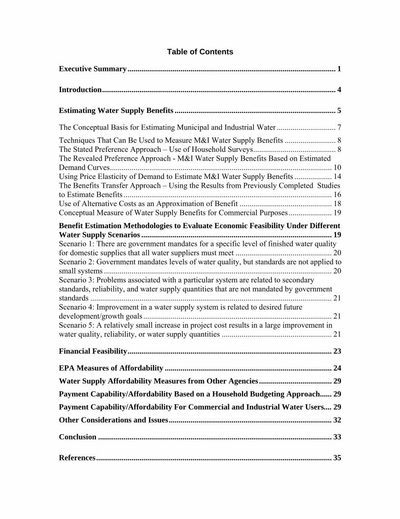
Table of Contents

Executive Summary .......................................................................................................... 1

Introduction ....................................................................................................................... 4

Estimating Water Supply Benefits .................................................................................. 5

The Conceptual Basis for Estimating Municipal and Industrial Water .............................. 7

Techniques That Can Be Used to Measure M&I Water Supply Benefits .......................... 8 The Stated Preference Approach – Use of Household Surveys .......................................... 8 The Revealed Preference Approach - M&I Water Supply Benefits Based on Estimated Demand Curves ................................................................................................................. 10 Using Price Elasticity of Demand to Estimate M&I Water Supply Benefits ................... 14 The Benefits Transfer Approach – Using the Results from Previously Completed Studies to Estimate Benefits .......................................................................................................... 16 Use of Alternative Costs as an Approximation of Benefit ............................................... 18 Conceptual Measure of Water Supply Benefits for Commercial Purposes ...................... 19

Benefit Estimation Methodologies to Evaluate Economic Feasibility Under Different Water Supply Scenarios ................................................................................................. 19 Scenario 1: There are government mandates for a specific level of finished water quality for domestic supplies that all water suppliers must meet ................................................. 20 Scenario 2: Government mandates levels of water quality, but standards are not applied to small systems .................................................................................................................... 20 Scenario 3: Problems associated with a particular system are related to secondary standards, reliability, and water supply quantities that are not mandated by government standards ........................................................................................................................... 21 Scenario 4: Improvement in a water supply system is related to desired future development/growth goals ................................................................................................ 21 Scenario 5: A relatively small increase in project cost results in a large improvement in water quality, reliability, or water supply quantities ........................................................ 21

Financial Feasibility ........................................................................................................ 23

EPA Measures of Affordability ..................................................................................... 24

Water Supply Affordability Measures from Other Agencies ..................................... 29

Payment Capability/Affordability Based on a Household Budgeting Approach...... 29

Payment Capability/Affordability For Commercial and Industrial Water Users.... 29

Other Considerations and Issues ................................................................................... 32

Conclusion ....................................................................................................................... 33

References ........................................................................................................................ 35

1

Executive Summary This document describes the basic concepts behind the determination of the economic and financial feasibility of municipal and industrial water supply improvements and the methods that can be used to evaluate economic and financial feasibility. The steps required to complete each type of analysis are presented. The strengths and shortcomings of the methods, different situations under which use of each method is most appropriate, and how the analyses can help in the planning process are also discussed. Economic and financial feasibility are two fundamentally different concepts. An analysis of economic feasibility evaluates the value of a water supply to society and answers the question: • Do the benefits of improved municipal and industrial water supply improvements exceed the costs of the improvements? An analysis of financial feasibility addresses the ability of water users to pay for water supply improvements and answers the questions: • How much can water users afford to pay for municipal and industrial water supply improvements? and • Is that amount sufficient to pay for a water supply improvement that is under consideration? Economic feasibility requires estimation of project benefits and costs. However, this document focuses on the methods that can be used to estimate the benefits of a municipal and industrial water supply because benefits are generally more difficult to quantify than costs. The primary costs associated with municipal and industrial water supply improvements are engineering costs that are relatively simple to identify and can be estimated using standard cost estimation procedures. It is recognized that some aspects of water supply project costs can be difficult to estimate—such as the environmental costs—but the valuation of these secondary costs is beyond the scope of this document. The benefits associated with the provision of improved municipal and industrial water supplies include direct benefits to the water users and indirect benefits to all of society. Indirect benefits are derived from the knowledge that a community that once did not have adequate water supplies and as a result suffered some type of hardship does not have to suffer that hardship with the project. Direct benefits to water users are easily identified but may be difficult to measure accurately. Indirect benefits are very difficult to identify and measure because they do not accrue to the water users themselves. A variety of approaches can be used to estimate the benefits from municipal and industrial water supply benefits. These approaches include:

2

• Stated preference approach – Based on the use of survey techniques to directly estimate benefits based on the willingness to pay for an improved water supply as stated by water users in a questionnaire. • Revealed preference approach - Based on actual observed behavior in market situations. The basic idea is that markets reveal the preferences of an individual through the price paid and the quantity purchased for a good or service. Market prices can be used to estimate willingness to pay functions from which benefits can be estimated. • Use of price elasticity estimates – Using estimates of the price elasticity of demand for municipal water supplies along with current quantities and prices in the market to estimate a municipal water demand relationship. This demand relationship can then be used to estimate benefits. • Benefits transfer approach – Using the results from previously completed studies to estimate benefits at the study site under consideration. • Cost of the most likely alternative – Using the resource cost of the water supply alternative that would be implemented in the absence of the project under consideration as an estimate of benefits. Each of the above approaches to estimating benefits are described in this document, recognizing that each has advantages and disadvantages that influence which method is most appropriate for a particular situation. The advantages and disadvantages are described in terms of the complexity in applying the method and accuracy of the estimates. The advantages and disadvantages are summarized in Table ES-1. The most appropriate methodology for evaluating the economic feasibility of an M&I project depends on the motivation for the project. If the project is required to meet mandated water quality or reliability standards, then a cost effectiveness based analysis such as the cost of the most likely alternative may provide the information necessary to make a sound economic choice between alternatives. If standards are not mandated, then a more rigorous analysis of benefits and costs may be needed to determine economic feasibility and to make a sound economic choice between alternatives. Financial feasibility focuses on the affordability of water supply improvements for water users. This document presents techniques that can be used to evaluate the affordability of municipal and industrial water supplies. Each of the affordability evaluation techniques discussed in this paper simplify the relationship between the ability of households or businesses to pay for water and the resources available to purchase necessary goods, services, and production inputs. For some techniques a simplifying assumption is made that the ability to pay for water is a constant percentage of household income for all income categories, while for other techniques the relationship is assumed to vary according to changes in socio-economic variables.

3

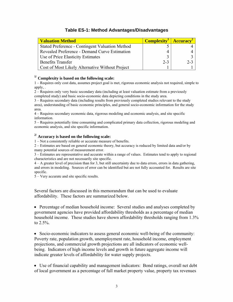
Table ES-1: Method Advantages/Disadvantages

Valuation Method Complexity1 Accuracy2

Stated Preference - Contingent Valuation Method Revealed Preference - Demand Curve Estimation Use of Price Elasticity Estimates Benefits Transfer Cost of Most Likely Alternative Without Project

5 4 3

2-3 1

443

2-31

1/ Complexity is based on the following scale: 1 – Requires only cost data, assumes project goal is met, rigorous economic analysis not required, simple to apply, . 2 – Requires only very basic secondary data (including at least valuation estimate from a previously completed study) and basic socio-economic data depicting conditions in the study area. 3 – Requires secondary data (including results from previously completed studies relevant to the study area), understanding of basic economic principles, and general socio-economic information for the study area. 4 – Requires secondary economic data, rigorous modeling and economic analysis, and site specific information. 5 – Requires potentially time consuming and complicated primary data collection, rigorous modeling and economic analysis, and site specific information. 2/ Accuracy is based on the following scale: 1 – Not a consistently reliable or accurate measure of benefits. 2 – Estimates are based on general economic theory, but accuracy is reduced by limited data and/or by many potential sources of measurement error. 3 – Estimates are representative and accurate within a range of values. Estimates tend to apply to regional characteristics and are not necessarily site specific. 4 – A greater level of precision than for 3, but still uncertainty due to data errors, errors in data gathering, and errors in modeling. Sources of error can be identified but are not fully accounted for. Results are site specific. 5 – Very accurate and site specific results. Several factors are discussed in this memorandum that can be used to evaluate affordability. These factors are summarized below. • Percentage of median household income: Several studies and analyses completed by government agencies have provided affordability thresholds as a percentage of median household income. These studies have shown affordability thresholds ranging from 1.3% to 2.5%. • Socio-economic indicators to assess general economic well-being of the community: Poverty rate, population growth, unemployment rate, household income, employment projections, and commercial growth projections are all indicators of economic well-being. Indicators of high income levels and growth in future aggregate income will indicate greater levels of affordability for water supply projects. • Use of financial capability and management indicators: Bond ratings, overall net debt of local government as a percentage of full market property value, property tax revenues

4

as a percentage of full market value of property, and the property tax collection rate are measures of available financial resources. The first three indicators are a measure of the ability to raise funds and the property tax burden. The collection rate is a measure of the efficiency of the tax collection system and the acceptability of given tax levels to residents. Indicators of high financial capability and good debt management improve financial capability estimates. • Use of the percentage increase in rates represented by the project costs: The percentage increase in rates that would occur if a water supply project is built is an indicator of the increased burden imposed on water users from the project. Studies have indicated that a short run rate increase that results in a 25% increase in original water bills for areas with already high water rates is one threshold for affordability and a 200% increase in original bills is another affordability threshold for areas with low water rates. High and low water rates should be considered relative to the overall cost of living and household income in a particular area. • Use of household budgeting techniques to evaluate water supply costs as a percentage of disposable household income. Percentages are estimated for the study area and for various communities and rural water districts in the same general region. The non-study area communities and study area results are compared to determine if water costs as a proportion of disposable income in the study area is substantially greater than for other areas in the same general region. The highest water payment percentages can be used to help assess affordability thresholds based on the assumption that the highest payment rates, while affordable, may approach maximum payment capability. The major drawback is that the highest observed rate may still not be the absolute maximum that can be paid. • Use of cost of production estimates and representative estimates of rates of return on investment to assess net revenues available to pay for water by commercial/industrial water users. Financial feasibility should be rigorously evaluated in order to be reasonably assured that the burden of repaying project costs will not cause financial hardship to water users and project loans will be repaid. Introduction A theoretically sound basis for evaluating economic feasibility (National Economic Development or NED analysis) is needed to determine the desirability of building a municipal and industrial (M&I) water supply project and to avoid building a project that is not correctly sized or should not be built at all. An evaluation of economic feasibility must include reliable estimates of the economic benefits and costs of the project. If the benefits generated by an M&I project exceed project costs, then the project is considered to be economically feasible. These benefits may accrue directly to water users through increased water supplies, improved reliability, or improved water quality. Some benefits may also accrue to non-users from simply knowing an area with inadequate water

5

supplies will receive improved water service. However, these indirect benefits are very difficult to quantify in most cases. The costs of an M&I project include all engineering costs of construction, construction materials and equipment costs, annual operation and maintenance costs, and any environmental costs that may result from construction of a project or loss of water supplies in environmentally sensitive areas. Another important aspect of an M&I water project evaluation is financial feasibility. A project is considered financially feasible if the water users have the financial resources to pay for the project, including capital and operating costs. Payments are typically reflected through increases in water rates charged to water users. A project can be financially infeasible from a local perspective even though it is feasible from an economic standpoint. The opposite case is also possible, where a project is financially feasible but it is not economically feasible. This paper provides options for estimating the payment capability of water users for M&I water supply projects as a measure of financial feasibility. Estimating Water Supply Benefits The Economic and Environmental Principles and Guidelines for Water and Related Land Resources Implementation Studies or P&G’s (U.S. Water Resources Council, 1983) provide some general standards for estimating M&I water supply benefits. However, the P&G’s do not provide a discussion of the specific methodologies that can be used to estimate M&I water supply benefits. This document presents methods and provides specific guidance for estimating M&I water supply benefits under a wide range of conditions that is not included in the P&G’s. The approaches presented in this document to estimate M&I benefits include: • Stated preference approaches, including contingent valuation and conjoint analysis. Contingent valuation is based on discrete choice responses that reflect estimated willingness to pay. Conjoint analysis is based on survey responses to pick the most desirable alternative out of a set of alternatives that have a variety of characteristics. • A revealed preference approach where domestic water supply and demand relationships are estimated using observed market behavior and these relationships are then used to estimate changes in welfare from water supply changes. • Using price elasticity of demand estimates applicable to the study area along with current quantities and prices for water in the study area to derive a demand curve from which benefits can estimated. • A benefits transfer approach where the results from previously completed studies are used to estimate benefits at the study site under consideration. • A cost of the most likely alternative approach where the resource cost of the water supply alternative that would be implemented in the absence of the project under consideration is used as a proxy for water supply benefits. Section VII, part 1.7.2 of the P&G’s indicate that the general measurement standard for valuing goods and services is the willingness of users to pay for each increment of output

6

from a plan (U.S. Water Resources Council, 1983). Willingness to pay can be defined as the dollar amount that an individual or firm is willing to give up or pay to acquire a good or service. This measurement standard is applied to all water related resources, including M&I water supplies. Four alternative techniques for valuing output are identified in the P&G’s: 1) actual or simulated market price, 2) change in net income, 3) cost of the most likely alternative, and 4) administratively established values. While any of the four methods can be used to estimate water values, the preference indicated in the P&G’s is for a market based approach or a change in net income approach because they actually reflect willingness to pay. The actual or simulated price technique is presented recognizing that “it is not possible in most instances for the planner to measure the actual demand situation” and an analysis that approximates a representative market price can be used to estimate willingness to pay. This technique allows the use of market price as a measure of willingness to pay when that price reflects the marginal cost of water. In other words, if the price reflects a market clearing equilibrium, then that price is a measure of willingness to pay for the last increment of water provided. The stated preference, revealed preference, and price elasticity approaches all fit into the actual or simulated price measurement category. The change in net income technique is based on the recognition that the maximum amount water users would be willing to pay for water would equal the change in net revenue generated by that activity with the water input. This is the valuation method typically used to measure agricultural water supply benefits and is still a measure based on the concept of willingness to pay. The change in net income technique is most applicable to the measurement of commercial water supply benefits and is discussed briefly. The cost of the most likely alternative approach represents a fall back approach that can be used when direct measures of willingness to pay are not available. Using this method the benefits from a water supply project are approximated by the resource cost of the alternative most likely to be implemented in the absence of that plan. The most likely alternative is typically a structural alternative. However, the benefits of nonstructural measures can also be computed using the cost of the most likely alternative. Generally, the net benefits of nonstructural measures that alter water use cannot be measured effectively using the alternative cost approach because of potentially wide variations in the level of project output: “Because of this lack of comparability, the benefit from such use-altering nonstructural measures should not be based on the cost of the most likely alternative” (U.S. Water Resources Council, 1983). The problem of the lack of comparability between project outputs could also be applied to any range of alternatives, structural or nonstructural, that produce a wide variation in project output. The alternative cost technique is useful in completing a cost effectiveness analysis where a water supply improvement has been mandated by government agencies. However, the use of alternative costs is not a true measure of water supply benefits. The use of administratively established values assumes that these values are similar to the price that would occur in a freely operating market and are reasonable proxy values.

7

However, these values are representative of market values only if they are based on the type of actual or simulated price analyses discussed above. This approach is, therefore, actually a benefits transfer type of approach. The Conceptual Basis for Estimating Municipal and Industrial Water Supply Benefits Willingness to pay is the price (dollar amount) that a buyer is willing to give up (opportunity cost) to acquire a good or service. The willingness of consumers to pay for a reliable, good quality water supply depends on the satisfaction or utility they obtain from the service as well as the utility consumers obtain from all other goods and services, constrained by available income. Therefore, willingness to pay takes preferences and income constraints into account. Willingness to pay is reflected through the demand curve for that good or service. The supply curve for a good or service reflects the marginal cost of providing that service and represents the minimum price required to bring an additional unit of output into the market. Using willingness to pay as a measure of benefit presents some potential equity issues. First, willingness to pay is constrained by ability to pay, so households with high incomes will appear to place a higher value on water service than those with low incomes. This may conflict with some ideas of fairness or justice (Pearce, 1994). A second potential problem occurs if a water quality or supply problem is created by new households or businesses moving into a region. In this case using willingness to pay to measure benefits may be objectionable because of the perceived unfairness of requiring households adversely affected by others to help pay to solve the problem. It is important to realize that these issues are the result of equity or fairness concerns and are not issues with the use of willingness to pay as a theoretically correct measure of economic benefit. In addition to the equity issues presented above, there are also practical problems in measuring the willingness to pay of water users for a water supply. Due to limited information available on how much water users will pay for water supplies with differing levels of quality and reliability along with the non-competitive nature of some water supply markets, it may not be possible to derive a demand curve from actual market data. As a result, other techniques based on surveys or results from previous studies may need to be used. The benefits from the provision of a good or service can be approximated by consumer surplus and producer surplus. Consumer surplus is the difference between what consumers are willing to pay for a good or service (as reflected by the demand curve) and what that consumer actually has to pay (as reflected by the market price). Consumer surplus is represented as the area under the demand curve and above market price as shown by the lighter triangle in Figure 1.

8

Figure 1: Price Consumer and Consumer surplus (CS) Producer Surplus $22.50 Supply $15 Producer surplus (PS) $10 Demand 0 750 Quantity Economic benefits also accrue to producers of a good or service. For producers the area above the supply curve (which reflects the cost of producing the good or service) and below market price is a measure of benefit. Producer surplus is the difference between what a supplier is paid for a good or service and what it costs to supply the good and is represented by the darker triangle in Figure 1. The sum of consumer surplus and producer surplus provides a measure of the total economic benefit of a good or service. This concept is important to benefit-cost analysis and welfare economics. The relationship between willingness to pay and the demand curve allows the use of demand curves to measure the change in benefits to consumers that result from changes in price or output. Similarly, the supply curve provides a measure of changes in the cost of production from changes in output. It should be noted that in practice the net benefits from a change in output that occur as a result of a project are typically measured by estimating the total area under the demand curve between the quantities provided with and without a project and subtracting the total cost of the project (which is equivalent to the area under the supply curve between the quantities provided with and without the project). Figure 1 shows the total benefit to society for a hypothetical good or service. The supply curve in Figure 1 indicates that at a price of $10 per unit or less there are no producers who would be willing to provide that good or service and the demand curve indicates at a price of $22.50 or higher there are no consumers who are willing to pay that price for the good or service (choke price). Consumer surplus (CS, which is the lighter triangle) is equal to: CS = ½ * ($7.50 * 750) or $2,812.50. The value of $7.50 is equal to the equilibrium price subtracted from the choke price. Producer surplus (PS, the darker triangle) is equal to: PS = ½ * ($5.00 * 750) or $1,875. The value of $5.00 is equal to the price at which there is no production subtracted from the equilibrium price. The total benefits from the provision of this good are equal to CS + PS or $4,687.50. Techniques That Can Be Used to Measure M&I Water Supply Benefits The Stated Preference Approach – Surveys of Water Users The stated preference approach can be used to directly estimate M&I water supply benefits based on preferences reflected through responses to water user surveys. There

9

are two methods that can be used to estimate natural resource values in terms of stated preferences, the contingent valuation method (CVM) and conjoint analysis (CA). The two methods are similar in that they are based on the use of surveys to estimate willingness to pay. However, the two methods are different in the way the goods and services being valued are presented in the survey questionnaires and how substitutions and tradeoffs that occur between goods and services are taken into account. The differences in the two methods can lead to a divergence in the estimates of willingness to pay using CVM and CA. The benefits from a water supply improvement can be measured using either CVM or CA by 1) asking water users their willingness to pay for increased water supplies, improved reliability of service or improved water quality (CVM), or 2) by presenting a range of scenarios that include different characteristics (including cost) and asking for a ranking of scenarios (CA). There are some potential advantages with CA, including the ability to describe preferences for many characteristics rather than making a with versus without comparison for one characteristic as is done with CVM. In addition, there may some improvement in statistical efficiency using CA. However, the statistical analysis is somewhat more complicated using CA and the format may make the survey questionnaires more difficult for respondents to answer. Since the basic approach to CVM and CA are similar and the main differences in the approaches apply to assumptions regarding the best way to frame questions to accurately reflect preferences and statistically model those preferences, only the CVM is discussed in detail below. The same general methodology applies to CA as well. CVM and CA use survey responses to questions regarding water supply characteristics with and without a project to measure the willingness to pay for a proposed change in the quantity or quality of the supply. A hypothetical demand curve is then constructed which can be used to estimate the benefits of the proposed water supply improvement. In the case of a CVM analysis the average willingness to pay from the surveys can be used to estimate benefits. Measurement of benefits using CVM is contingent upon the survey respondent understanding the proposed improvement and their ability to place a value on the improvement described in the survey or in the case of CA the ability of the respondent to make comparisons between scenarios. For example, the benefits to water users from converting from groundwater to surface water supplies could be estimated using CVM by asking users their willingness to pay for a surface water project or using CA by presenting a range of scenarios with different water supply characteristics and asking for a ranking of scenarios. However, water users must understand how the conversion to surface water will affect water quality and reliability and the water users must be able place a monetary value on the change in terms of what water users are willing to give up (opportunity cost) to get the water supply change. For CVM or CA to produce reliable and unbiased estimates of resource values, survey respondents must be familiar with the good they are valuing and they must understand the proposed change in the resource. CVM is likely to provide representative benefit estimates for municipal and industrial water supply improvements compared to some

10

other resource values because of the familiarity of water users with water supply problems and the familiarity with potential solutions to these problems such as pipelines and water treatment facilities. The general steps that need to be followed when using CVM to estimating M&I benefits include: Step 1: Determine the water supply conditions that will exist for each alternative under consideration, including a no-action alternative. This becomes the basis for describing what survey respondents will be “buying.” This first step is not an economic activity but is an interdisciplinary activity where all resource impacts are evaluated. Step 2: Determine the geographic area that will be affected by the water supply improvement. This becomes the survey sampling area and represents consumers that will receive the water supply benefits. Step 3: Develop a survey questionnaire which includes a willingness to pay question with enough detail (as determined in Step 1) to allow the respondents to know what they are getting for their money. Questions also need to be included which represent variables that are expected to influence willingness to pay, such as income, household size, business size, type of business, etc. Step 4: Conduct a survey of a representative sample of the affected water supply population. Questionnaires may be sent in the mail, a telephone survey may be implemented, or a survey may be conducted through personal interviews. Step 5: Estimate an M&I benefit function based on the willingness to pay responses and responses to the other survey question data. There is disagreement among economists regarding the accuracy of benefit estimates derived from contingent valuation based analyses. Potential biases exist in the presentation of information in a survey, the hypothetical nature of contingent valuation questions, and the sampling methods used. However, CVM has been applied to a wide variety of resource valuation situations. These valuations have led to a better understanding of the accuracy and limits of the method and have provided little evidence of strategic behavior (Brookshire and McKee, 1994). The use of CVM has become a fairly well accepted methodology for estimating resource benefits and several studies have have used CVM to estimate water supply benefits (Powell and Allee, 1990; Shultz and Lindsay, 1990; Dahl, 1992; Jordan and Elnagheeb, 1993; Howe and Smith, 1994; Piper and Martin, 1997; and Piper, 1998). The Revealed Preference Approach - M&I Water Supply Benefits Based on Estimated Demand Curves The revealed preference approach is based on observed market behavior or behavior in “market like” conditions. These observations of how consumers react to changes in price can be used to estimate a demand curve from which benefits can be estimated. Observed price-quantity combinations in municipal water markets reveal consumer preferences and will reflect willingness to pay for various quantities of water.

11

Theoretically, if we know two price-quantity combinations that represent points on a demand curve, then a linear demand curve can be estimated. If a large number of observed market-clearing price-quantity combinations are known, then a more representative demand curve can be estimated and non-linear functional forms can be used. The supply curve can be estimated in a similar manner, showing price and quantity supplied combinations. It should be noted that a municipal water supply curve may be nearly horizontal, especially for incremental increases in the quantity supplied for systems that can be fairly easily expanded. A horizontal supply curve indicates that the marginal cost of additional supplies is constant. While this may not be the case for small quantities of water supplied, it is likely to be nearly horizontal for large quantities when economies of scale are realized. Once the demand and supply curves are identified, the benefits associated with incremental changes in quantity can be estimated. M&I demand curves can be estimated using time series data, cross-sectional data, or both. Time series data involves the use of data for a single entity over a period of time while cross-sectional data refers to data collected for many entities at one point in time or over a short period of time. It is generally more difficult to obtain a sufficient number of observations to estimate an M&I water demand curve using time series data for a water provider than for cross-sectional data for several water providers. Therefore, cross-sectional price and quantity information from various municipalities and rural water systems in the region of interest may be the best source of data for estimating M&I water demand curves. In order to estimate a household demand curve, data are needed for water price, the quantity of water purchased, income, household size, climate variables, and any other variables that would be expected to influence the quantity of water demanded. A demand curve for commercial water supplies would include price and quantity variables, along with a type of good or service variable that would indicate the importance of water as a production input, number of employees as a measure of business size, revenues, climate variables, and any other variables that would be expected to influence the quantity of water demanded. It should be recognized that there are potential difficulties involved in estimating generalized demand curves using cross-sectional data. First, water price and quantity information obtained from each water provider represent averages actually observed for each provider. Therefore, an aggregated demand curve based on averages from each provider will portray a representative demand relationship but will not portray a precise relationship for the specific site being studied. Second, it must be assumed that each price-quantity combination represents a market clearing equilibrium. If the price of water is administratively set at a level that is lower than the equilibrium market price, then that price-quantity observation would not represent a point on the demand curve and will introduce bias in the estimated demand curve. A simplified residential water example of a revealed preference type of analysis based on estimation of a regional water demand curve is shown below.

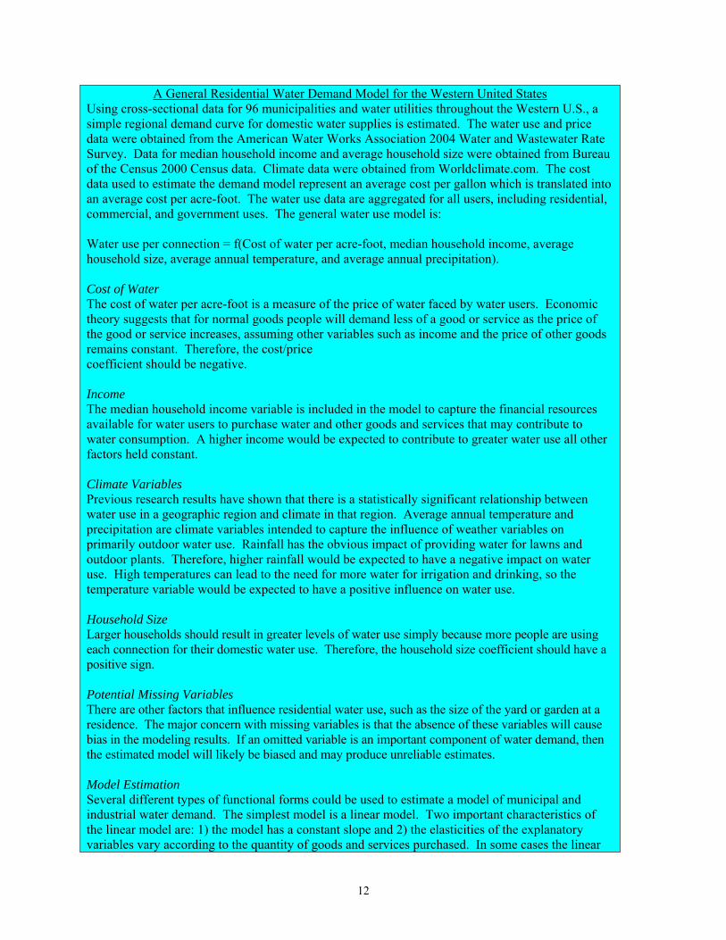
12

A General Residential Water Demand Model for the Western United States Using cross-sectional data for 96 municipalities and water utilities throughout the Western U.S., a simple regional demand curve for domestic water supplies is estimated. The water use and price data were obtained from the American Water Works Association 2004 Water and Wastewater Rate Survey. Data for median household income and average household size were obtained from Bureau of the Census 2000 Census data. Climate data were obtained from Worldclimate.com. The cost data used to estimate the demand model represent an average cost per gallon which is translated into an average cost per acre-foot. The water use data are aggregated for all users, including residential, commercial, and government uses. The general water use model is: Water use per connection = f(Cost of water per acre-foot, median household income, average household size, average annual temperature, and average annual precipitation). Cost of Water The cost of water per acre-foot is a measure of the price of water faced by water users. Economic theory suggests that for normal goods people will demand less of a good or service as the price of the good or service increases, assuming other variables such as income and the price of other goods remains constant. Therefore, the cost/price coefficient should be negative. Income The median household income variable is included in the model to capture the financial resources available for water users to purchase water and other goods and services that may contribute to water consumption. A higher income would be expected to contribute to greater water use all other factors held constant. Climate Variables Previous research results have shown that there is a statistically significant relationship between water use in a geographic region and climate in that region. Average annual temperature and precipitation are climate variables intended to capture the influence of weather variables on primarily outdoor water use. Rainfall has the obvious impact of providing water for lawns and outdoor plants. Therefore, higher rainfall would be expected to have a negative impact on water use. High temperatures can lead to the need for more water for irrigation and drinking, so the temperature variable would be expected to have a positive influence on water use. Household Size Larger households should result in greater levels of water use simply because more people are using each connection for their domestic water use. Therefore, the household size coefficient should have a positive sign. Potential Missing Variables There are other factors that influence residential water use, such as the size of the yard or garden at a residence. The major concern with missing variables is that the absence of these variables will cause bias in the modeling results. If an omitted variable is an important component of water demand, then the estimated model will likely be biased and may produce unreliable estimates. Model Estimation Several different types of functional forms could be used to estimate a model of municipal and industrial water demand. The simplest model is a linear model. Two important characteristics of the linear model are: 1) the model has a constant slope and 2) the elasticities of the explanatory variables vary according to the quantity of goods and services purchased. In some cases the linear

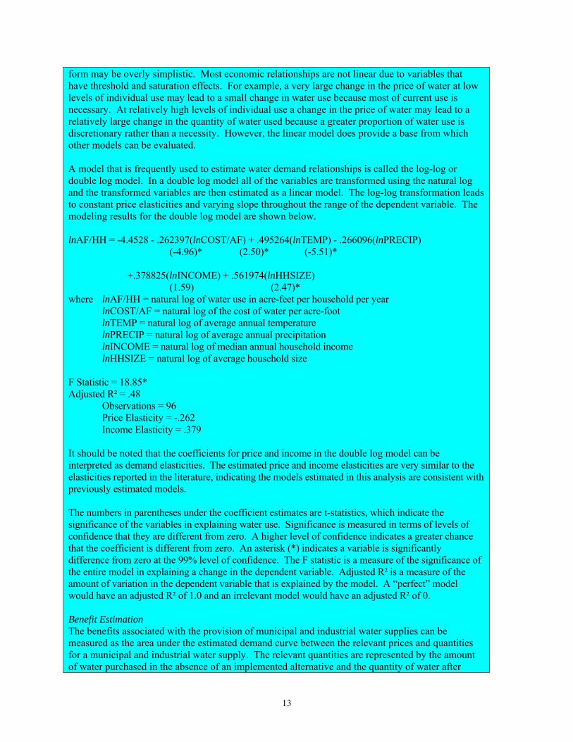
13

form may be overly simplistic. Most economic relationships are not linear due to variables that have threshold and saturation effects. For example, a very large change in the price of water at low levels of individual use may lead to a small change in water use because most of current use is necessary. At relatively high levels of individual use a change in the price of water may lead to a relatively large change in the quantity of water used because a greater proportion of water use is discretionary rather than a necessity. However, the linear model does provide a base from which other models can be evaluated. A model that is frequently used to estimate water demand relationships is called the log-log or double log model. In a double log model all of the variables are transformed using the natural log and the transformed variables are then estimated as a linear model. The log-log transformation leads to constant price elasticities and varying slope throughout the range of the dependent variable. The modeling results for the double log model are shown below. lnAF/HH = -4.4528 - .262397(lnCOST/AF) + .495264(lnTEMP) - .266096(lnPRECIP) (-4.96)* (2.50)* (-5.51)* +.378825(lnINCOME) + .561974(lnHHSIZE) (1.59) (2.47)* where lnAF/HH = natural log of water use in acre-feet per household per year lnCOST/AF = natural log of the cost of water per acre-foot lnTEMP = natural log of average annual temperature lnPRECIP = natural log of average annual precipitation lnINCOME = natural log of median annual household income lnHHSIZE = natural log of average household size F Statistic = 18.85* Adjusted R² = .48 Observations = 96 Price Elasticity = -.262 Income Elasticity = .379 It should be noted that the coefficients for price and income in the double log model can be interpreted as demand elasticities. The estimated price and income elasticities are very similar to the elasticities reported in the literature, indicating the models estimated in this analysis are consistent with previously estimated models. The numbers in parentheses under the coefficient estimates are t-statistics, which indicate the significance of the variables in explaining water use. Significance is measured in terms of levels of confidence that they are different from zero. A higher level of confidence indicates a greater chance that the coefficient is different from zero. An asterisk (*) indicates a variable is significantly difference from zero at the 99% level of confidence. The F statistic is a measure of the significance of the entire model in explaining a change in the dependent variable. Adjusted R² is a measure of the amount of variation in the dependent variable that is explained by the model. A “perfect” model would have an adjusted R² of 1.0 and an irrelevant model would have an adjusted R² of 0. Benefit Estimation The benefits associated with the provision of municipal and industrial water supplies can be measured as the area under the estimated demand curve between the relevant prices and quantities for a municipal and industrial water supply. The relevant quantities are represented by the amount of water purchased in the absence of an implemented alternative and the quantity of water after

14

implementing an alternative. The relevant quantities of water with and without an alternative cannot be known with certainty because future population growth, growth in commercial/industrial water demands, and future socio-economic conditions cannot be known with certainty. The quantities of water used in an analysis to evaluate water supply benefits should be based on the estimated water use with and without an alternative under consideration or the available water supplies available that meet some specific criteria with or without an alternative. This information is necessary, along with representative values for the socio-economic variables included in the equation, in order to know the appropriate end points along the estimated demand curve from which benefits are derived. M&I water benefits can then be estimated by integrating the estimated demand equation and solving for the area under the demand curve between the price/quantity combinations with and without an implemented alternative.

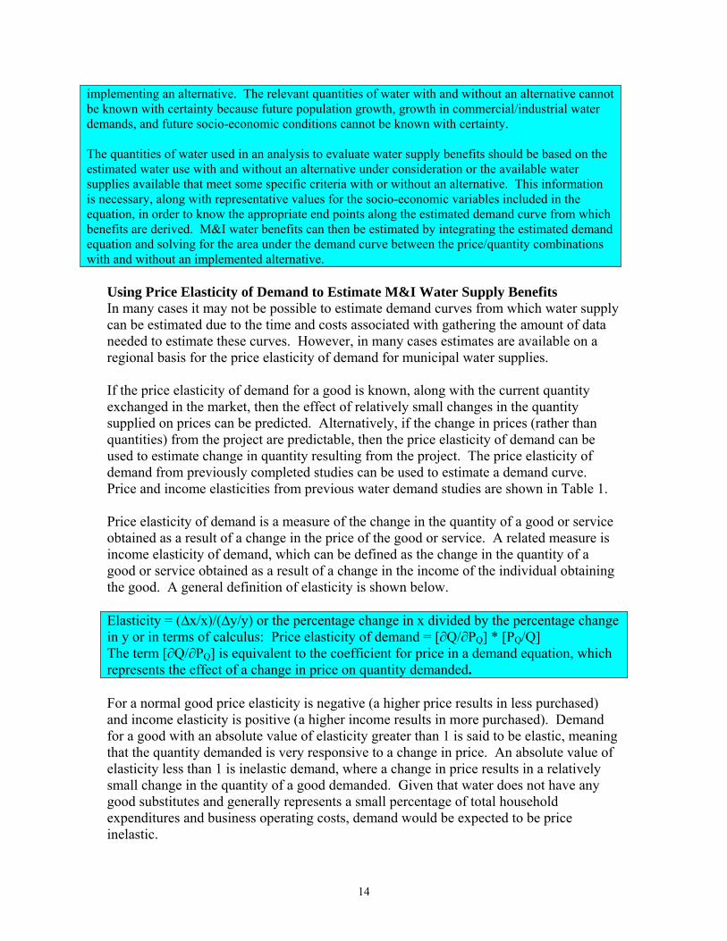
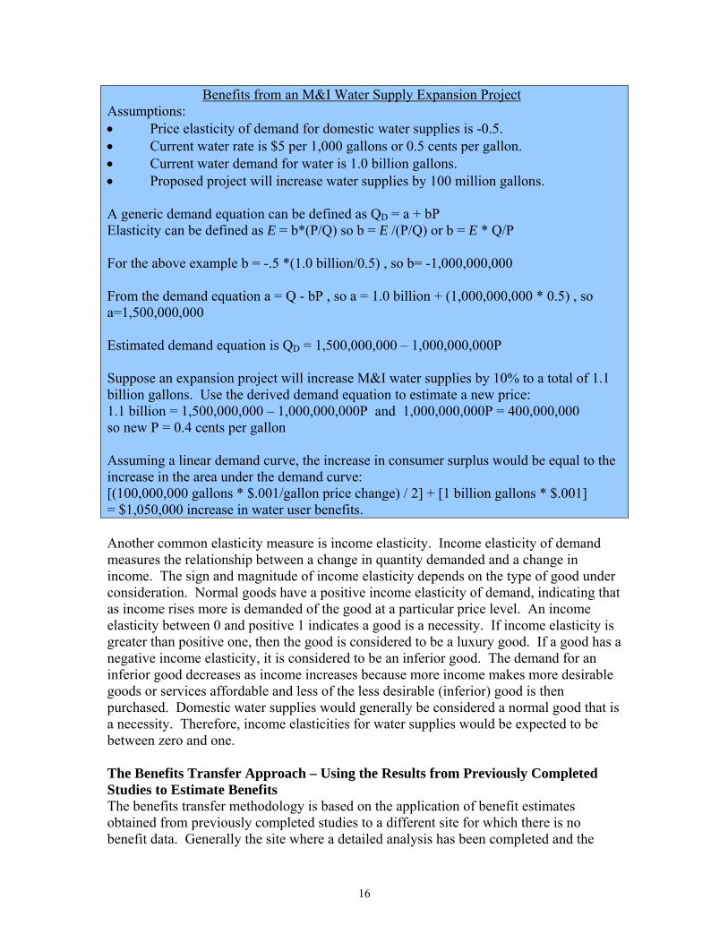
Using Price Elasticity of Demand to Estimate M&I Water Supply Benefits In many cases it may not be possible to estimate demand curves from which water supply can be estimated due to the time and costs associated with gathering the amount of data needed to estimate these curves. However, in many cases estimates are available on a regional basis for the price elasticity of demand for municipal water supplies.

If the price elasticity of demand for a good is known, along with the current quantity exchanged in the market, then the effect of relatively small changes in the quantity supplied on prices can be predicted. Alternatively, if the change in prices (rather than quantities) from the project are predictable, then the price elasticity of demand can be used to estimate change in quantity resulting from the project. The price elasticity of demand from previously completed studies can be used to estimate a demand curve. Price and income elasticities from previous water demand studies are shown in Table 1. Price elasticity of demand is a measure of the change in the quantity of a good or service obtained as a result of a change in the price of the good or service. A related measure is income elasticity of demand, which can be defined as the change in the quantity of a good or service obtained as a result of a change in the income of the individual obtaining the good. A general definition of elasticity is shown below. Elasticity = (∆x/x)/(∆y/y) or the percentage change in x divided by the percentage change in y or in terms of calculus: Price elasticity of demand = [∂Q/∂PQ] * [PQ/Q] The term [∂Q/∂PQ] is equivalent to the coefficient for price in a demand equation, which represents the effect of a change in price on quantity demanded. For a normal good price elasticity is negative (a higher price results in less purchased) and income elasticity is positive (a higher income results in more purchased). Demand for a good with an absolute value of elasticity greater than 1 is said to be elastic, meaning that the quantity demanded is very responsive to a change in price. An absolute value of elasticity less than 1 is inelastic demand, where a change in price results in a relatively small change in the quantity of a good demanded. Given that water does not have any good substitutes and generally represents a small percentage of total household expenditures and business operating costs, demand would be expected to be price inelastic.

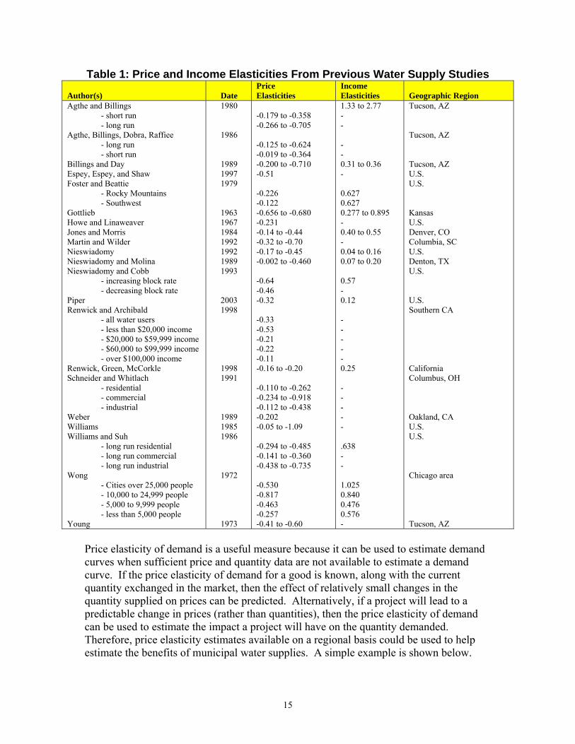
15

Table 1: Price and Income Elasticities From Previous Water Supply Studies Author(s)

Date

Price Elasticities

Income Elasticities

Geographic Region

Agthe and Billings - short run - long run Agthe, Billings, Dobra, Raffiee - long run - short run Billings and Day Espey, Espey, and Shaw Foster and Beattie - Rocky Mountains - Southwest Gottlieb Howe and Linaweaver Jones and Morris Martin and Wilder Nieswiadomy Nieswiadomy and Molina Nieswiadomy and Cobb - increasing block rate - decreasing block rate Piper Renwick and Archibald - all water users - less than $20,000 income - $20,000 to $59,999 income - $60,000 to $99,999 income - over $100,000 income Renwick, Green, McCorkle Schneider and Whitlach - residential - commercial - industrial Weber Williams Williams and Suh - long run residential - long run commercial - long run industrial Wong - Cities over 25,000 people - 10,000 to 24,999 people - 5,000 to 9,999 people - less than 5,000 people Young

1980

1986

1989 1997 1979

1963 1967 1984 1992 1992 1989 1993

2003 1998

1998 1991

1989 1985 1986

1972

1973

-0.179 to -0.358 -0.266 to -0.705 -0.125 to -0.624 -0.019 to -0.364 -0.200 to -0.710 -0.51 -0.226 -0.122 -0.656 to -0.680 -0.231 -0.14 to -0.44 -0.32 to -0.70 -0.17 to -0.45 -0.002 to -0.460 -0.64 -0.46 -0.32 -0.33 -0.53 -0.21 -0.22 -0.11 -0.16 to -0.20 -0.110 to -0.262 -0.234 to -0.918 -0.112 to -0.438 -0.202 -0.05 to -1.09 -0.294 to -0.485 -0.141 to -0.360 -0.438 to -0.735 -0.530 -0.817 -0.463 -0.257 -0.41 to -0.60

1.33 to 2.77 - - - - 0.31 to 0.36 - 0.627 0.627 0.277 to 0.895 - 0.40 to 0.55 - 0.04 to 0.16 0.07 to 0.20 0.57 - 0.12 - - - - - 0.25 - - - - - .638 - - 1.025 0.840 0.476 0.576 -

Tucson, AZ Tucson, AZ Tucson, AZ U.S. U.S. Kansas U.S. Denver, CO Columbia, SC U.S. Denton, TX U.S. U.S. Southern CA California Columbus, OH Oakland, CA U.S. U.S. Chicago area Tucson, AZ

Price elasticity of demand is a useful measure because it can be used to estimate demand curves when sufficient price and quantity data are not available to estimate a demand curve. If the price elasticity of demand for a good is known, along with the current quantity exchanged in the market, then the effect of relatively small changes in the quantity supplied on prices can be predicted. Alternatively, if a project will lead to a predictable change in prices (rather than quantities), then the price elasticity of demand can be used to estimate the impact a project will have on the quantity demanded. Therefore, price elasticity estimates available on a regional basis could be used to help estimate the benefits of municipal water supplies. A simple example is shown below.

16

Benefits from an M&I Water Supply Expansion Project Assumptions: • Price elasticity of demand for domestic water supplies is -0.5. • Current water rate is $5 per 1,000 gallons or 0.5 cents per gallon. • Current water demand for water is 1.0 billion gallons. • Proposed project will increase water supplies by 100 million gallons. A generic demand equation can be defined as QD = a + bP Elasticity can be defined as E = b*(P/Q) so b = E /(P/Q) or b = E * Q/P For the above example b = -.5 *(1.0 billion/0.5) , so b= -1,000,000,000 From the demand equation a = Q - bP , so a = 1.0 billion + (1,000,000,000 * 0.5) , so a=1,500,000,000 Estimated demand equation is QD = 1,500,000,000 – 1,000,000,000P Suppose an expansion project will increase M&I water supplies by 10% to a total of 1.1 billion gallons. Use the derived demand equation to estimate a new price: 1.1 billion = 1,500,000,000 – 1,000,000,000P and 1,000,000,000P = 400,000,000 so new P = 0.4 cents per gallon Assuming a linear demand curve, the increase in consumer surplus would be equal to the increase in the area under the demand curve: [(100,000,000 gallons * $.001/gallon price change) / 2] + [1 billion gallons * $.001] = $1,050,000 increase in water user benefits. Another common elasticity measure is income elasticity. Income elasticity of demand measures the relationship between a change in quantity demanded and a change in income. The sign and magnitude of income elasticity depends on the type of good under consideration. Normal goods have a positive income elasticity of demand, indicating that as income rises more is demanded of the good at a particular price level. An income elasticity between 0 and positive 1 indicates a good is a necessity. If income elasticity is greater than positive one, then the good is considered to be a luxury good. If a good has a negative income elasticity, it is considered to be an inferior good. The demand for an inferior good decreases as income increases because more income makes more desirable goods or services affordable and less of the less desirable (inferior) good is then purchased. Domestic water supplies would generally be considered a normal good that is a necessity. Therefore, income elasticities for water supplies would be expected to be between zero and one. The Benefits Transfer Approach – Using the Results from Previously Completed Studies to Estimate Benefits The benefits transfer methodology is based on the application of benefit estimates obtained from previously completed studies to a different site for which there is no benefit data. Generally the site where a detailed analysis has been completed and the

17

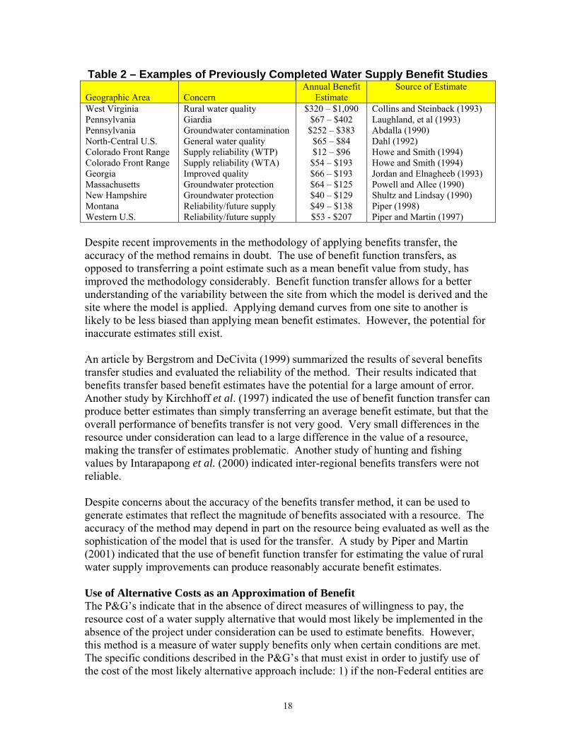
study site should have similar characteristics. Similarity can be defined in terms of economic conditions, population characteristics, resources within an area, and other socio-economic characteristics. The application of the benefit transfer method assumes that a general relationship exists between various socio-economic variables and the value of a resource. It is further assumed that this relationship can be estimated and applied to another geographic area. If these assumptions hold, then a model for a water supply that includes factors important in determining the value of municipal and industrial water can in theory be applied to another study site to estimate the benefits of a water supply improvement. Potential benefit transfer problems that must be considered include differences in water supply problems between sites and differences in socio-economic characteristics. The over-riding considerations in the application of a benefit transfer model are the applicability of the transferred model to the study site and the inclusion of all explanatory variables that are theoretically important. Some of the more important water supply benefit variables include: household size, age, income, cost of water, water quality, and the existence of any unusual hardship, such as the need to haul water or purchase bottled water for drinking. Household size can be a proxy for use and can also be a measure of water supply importance, where larger households represent greater dependence on supplies. Age may be a reflection of attitudes, where experience with problems and situations affects how people perceive and react to difficulties. Income reflects the resources available to spend on all goods and services purchased by the household. The cost of water indicates the current amount that must be spent for water at the current level of quality and reliability. Unusual hardships are an indication of the inconvenience associated with current water supplies. The variable values that should be used in the transferred benefit model should represent conditions at the study site under consideration. The value could be the mean, median, or some other number that is representative of the study area population. More than one value could be used as a sensitivity analysis. Once the representative values are input into the transferred model, M&I water supply benefits can be estimated. It is important to note that the quality of the estimates of benefits derived using benefits transfer are limited by the availability of technically sound water supply studies. A partial list of published studies estimating the benefits from improving or preserving domestic water quality and reliability are presented in Table 2. The studies cited in Table 1 in the discussion of elasticity also provide estimates of the value of water for domestic purposes. The models and benefit estimates in these studies, and other studies not listed in this report, can be used as a basis for benefit transfer analyses estimating the benefits from domestic water supply improvements.

18

Table 2 – Examples of Previously Completed Water Supply Benefit Studies Geographic Area

Concern

Annual Benefit Estimate

Source of Estimate

West Virginia Pennsylvania Pennsylvania North-Central U.S. Colorado Front Range Colorado Front Range Georgia Massachusetts New Hampshire Montana Western U.S.

Rural water quality Giardia Groundwater contamination General water quality Supply reliability (WTP) Supply reliability (WTA) Improved quality Groundwater protection Groundwater protection Reliability/future supply Reliability/future supply

$320 – $1,090 $67 – $402 $252 – $383 $65 – $84 $12 – $96

$54 – $193 $66 – $193 $64 – $125 $40 – $129 $49 – $138 $53 - $207

Collins and Steinback (1993) Laughland, et al (1993) Abdalla (1990) Dahl (1992) Howe and Smith (1994) Howe and Smith (1994) Jordan and Elnagheeb (1993) Powell and Allee (1990) Shultz and Lindsay (1990) Piper (1998) Piper and Martin (1997)

Despite recent improvements in the methodology of applying benefits transfer, the accuracy of the method remains in doubt. The use of benefit function transfers, as opposed to transferring a point estimate such as a mean benefit value from study, has improved the methodology considerably. Benefit function transfer allows for a better understanding of the variability between the site from which the model is derived and the site where the model is applied. Applying demand curves from one site to another is likely to be less biased than applying mean benefit estimates. However, the potential for inaccurate estimates still exist. An article by Bergstrom and DeCivita (1999) summarized the results of several benefits transfer studies and evaluated the reliability of the method. Their results indicated that benefits transfer based benefit estimates have the potential for a large amount of error. Another study by Kirchhoff et al. (1997) indicated the use of benefit function transfer can produce better estimates than simply transferring an average benefit estimate, but that the overall performance of benefits transfer is not very good. Very small differences in the resource under consideration can lead to a large difference in the value of a resource, making the transfer of estimates problematic. Another study of hunting and fishing values by Intarapapong et al. (2000) indicated inter-regional benefits transfers were not reliable. Despite concerns about the accuracy of the benefits transfer method, it can be used to generate estimates that reflect the magnitude of benefits associated with a resource. The accuracy of the method may depend in part on the resource being evaluated as well as the sophistication of the model that is used for the transfer. A study by Piper and Martin (2001) indicated that the use of benefit function transfer for estimating the value of rural water supply improvements can produce reasonably accurate benefit estimates. Use of Alternative Costs as an Approximation of Benefit The P&G’s indicate that in the absence of direct measures of willingness to pay, the resource cost of a water supply alternative that would most likely be implemented in the absence of the project under consideration can be used to estimate benefits. However, this method is a measure of water supply benefits only when certain conditions are met. The specific conditions described in the P&G’s that must exist in order to justify use of the cost of the most likely alternative approach include: 1) if the non-Federal entities are

19

likely to provide similar output in the absence of any of the alternative plans under consideration, and 2) if NED benefits cannot be estimated from market price or change in net income. The P&G’s also state “Estimates of benefit should be based on the cost of the most likely alternative only if there is evidence that the alternative would be implemented.” In other words, the procedure should only be used in cases where preferences for an alternative that would provide a service are revealed to support the alternative. This prevents the use of the procedure when the alternative is much more expensive than could reasonably be supported by the affected parties to justify a project. The most likely alternative should give adequate consideration to nonstructural and demand management measures as well as structural measures. Demand management measures would consider conservation activities that increase water system efficiencies, prioritize water uses, and any other activities that would reduce water supply demands and decrease the need for expanded supply alternatives. It should be noted that the cost of demand management measures have the potential to be considerably lower cost than supply expansion alternatives. If a demand management alternative would be the most likely alternative implemented in the absence of the preferred plan, then the relatively low cost of the demand management alternative would be identified as the benefit. This approach is an approximation of water supply benefits only under very restrictive conditions. Conceptual Measure of Water Supply Benefits for Commercial Purposes The value of water for commercial purposes is conceptually a little easier to measure than the value to households. The net value added from commercial output attributable to a water supply improvement is a measure of benefit. The techniques discussed above can also be applied to commercial water users. However, commercial benefits can also be estimated as the difference in the net value of output with the water supply minus the net value of output without the water supply. For example, suppose a computer chip manufacturer can produce $1 million worth of chips at a cost of $500,000 with their current water supply. Also suppose that the manufacturer could produce $2 million worth of chips at a cost of $750,000 with an improved water supply. The benefit of the new water supply to the chip manufacturer would be calculated as $1.25 million ($2 million minus $750,000) minus $500,000 ($1 million minus $500,000), or $750,000. This could then be converted into benefits per acre-foot by dividing $750,000 by the number of acre-feet of water used by the chip manufacturer. Benefit Estimation Methodologies to Evaluate Economic Feasibility Under Different Water Supply Scenarios Four different scenarios are presented below under which different methods of estimating M&I benefits are theoretically justified. More than one methodology can be used for each of the scenarios described. The method that meets minimum standards for validity and accuracy are identified for each scenario. Methods that can provide more precise benefit estimates are also indicated.

20

Scenario 1: There are government mandates for a specific level of finished water quality for domestic supplies that all water suppliers must meet. In this scenario mandated water quality standards are universally set based on the estimated risk associated with different levels of a pollutant. These standards are typically measured as maximum acceptable levels for very specific pollutants or indicators of pollutants. Implementation of these standards assumes that the costs of those risks above the maximum acceptable level are too high in terms of mortality, chronic illness, or other damages. Given this assumption, it follows that the benefits from improved water quality measured in terms of reduced mortality, illness, and other damages are greater than the costs of meeting the mandated level in water quality. If this was not the case, then the policy decision to implement water quality standards would not be made. In other words, implementing the standards implies the benefits of improved water quality exceed the costs of the improvement. Under this restrictive scenario net benefits will be maximized when the lowest cost method of attaining the standard is implemented, assuming each alternative meets the mandated standard. This is the equivalent of the alternative cost procedure discussed in the P&G’s. For this scenario the economic analysis becomes relatively simple, where the economically justified alternative is the least cost alternative that meets the water quality standard. The benefit analysis becomes a cost effectiveness analysis. However, it must be recognized that if the policy decision is in fact not correct (for example, meeting the standard really has no effect or an insignificant effect on health), then the least cost analysis will not identify an alternative that generates net positive economic benefits. To a large extent a cost-effectiveness analysis becomes a simple accounting exercise where the costs must be properly valued. This involves the use of a discount rate, assessing cost trends, accurately estimating operation and maintenance costs, and accounting for any other factors that would influence costs. While estimating costs may not be a trivial exercise, the analysis is simplified tremendously by the assumption that benefits exceed costs. If there is concern that the true benefits from water supply improvements are less than the costs of the least cost alternative, then a more rigorous analysis using any of the other four benefit estimation techniques would be warranted. The estimated benefits as measured by willingness to pay, rather than as estimated by resource cost, could then be compared to project costs. Scenario 2: Government mandates levels of water quality, but standards are not applied to small systems. In this scenario it is implicitly assumed that the level of benefits associated with meeting water quality goals for large systems are sufficient to justify the costs of meeting the standards. However, the level of benefit is not necessarily large enough to cover the costs of compliance for smaller systems as indicated by application to only large systems. Greater benefits to larger systems could simply be the result of economies of scale, where large systems can use a high cost technology to meet a standard and spread those costs over a large user base. The cost per user may be relatively small and benefits derived from a large number of users may be relatively

21

large. The same high cost technology may be too expensive for smaller systems that would have to pass on the high costs and would derive relatively low benefits from a small customer base. For this scenario, the analysis for the larger system could be carried out in the same way as for Scenario 1, where the lowest cost alternative that meets the standard for water users would generate the greatest net benefit. However, for the small systems where it is not universally assumed that the benefits are greater than the costs, the net benefits of a water supply improvement cannot be assumed to be maximized with the least cost alternative. If the costs of any proposed system improvement are actually greater than the benefits, then the best project from an economic perspective would be no project. An economic evaluation of the small systems would require estimates of the benefits and costs of each water supply alternative and the theoretically appropriate measure of benefit is the willingness to pay for the water supply improvement. If the costs associated with a large project are very high and the analyst is concerned that the true benefits are not greater than the costs, then a measure of willingness to pay may be needed for the large project as well. Scenario 3: Problems associated with a particular system are related to secondary standards, reliability, and water supply quantities that are not mandated by government standards. In this case a cost comparison of the various alternatives cannot be used for economic justification of the project. If there are no regulatory mandates associated with a proposed improvement from which it can be assumed project benefits at least equal costs, then the willingness to pay for the improvements must be estimated to complete a valid analysis of economic feasibility. Under this scenario an analysis of costs will not guarantee that any alternative is economically feasible, even if it is the lowest cost compared to all other alternatives. Under this scenario a complete benefit/cost analysis should be completed using one of the economic benefit evaluation techniques described above that estimates willingness to pay. Each alternative must be evaluated on its own merit, where the benefits are dependent on the ability of each alternative to improve the current water supply situation. If an alternative is very expensive, then it is very important to carefully measure the benefits as accurately as possible to justify large expenditures. It is also important to accurately measure benefits in cases where the costs of all the alternatives are similar or it is suspected that the benefits and costs are of a similar magnitude. If the measured benefits are small, then even a low cost alternative may be too expensive to generate positive net benefits. If the estimated benefits are large enough to cover the costs of a project, then the project is economically feasible and we can move to the question of financial feasibility. Scenario 4: Improvement in a water supply system is related to desired future development/growth goals. This scenario is more difficult to evaluate than the third scenario. In this scenario, there may not be any measurable benefit from any of the project alternatives given the current conditions (there are no supply shortages and water quality is acceptable), but future benefits are expected or desired. These future benefits

22

may be very difficult to measure because the extent to which future water users would benefit is not yet known. The benefits of providing M&I water to future users could be estimated by asking current users their willingness to pay for that expansion as part of a contingent valuation study. However, many current water users may not support future development and population growth and as a result understate the benefits of expanding water supplies to support future growth. In order to avoid potential bias in contingent valuation based benefit estimates, willingness to pay for water as measured using one of the other three methods discussed previously may be estimated for the current water users. The average benefit for current water users can then be assumed to apply to future water users. Project benefits could then be estimated by multiplying the benefit per household/commercial establishment times the projected number of water users in the future. Scenario 5: A relatively small increase in project cost results in a large improvement in water quality, reliability, or water supply quantities. In this case it is assumed that all alternatives under consideration meet a documented level of need or meet a water quality goal, which may or may not be based on a regulatory mandate, but that at least one alternative exceeds the minimum requirement. It is also assumed that at least one alternative that exceeds the minimum requirement can do so at a relatively low additional cost compared to the least cost alternative. Under this scenario a modification of the alternative cost method based on incremental costs and benefits can be used to identify the cost effectiveness of attaining additional benefits. The incremental cost comparison simply measures the additional cost per unit of improvement. The additional cost per unit can then be compared to the average cost per unit of improvement for the other alternatives that meet the minimum requirements to determine if the additional benefit is obtained at a lower per unit price. The incremental cost approach provides good information on the relative cost of incremental improvements, but does not prove economic feasibility. If the benefits are not measured in economic terms that are directly comparable to costs, it cannot be known if the benefits of the additional improvement actually exceed the costs. An analysis of costs will not guarantee that any alternative is economically feasible. A complete benefit/cost analysis should be completed under this scenario using one of the economic benefit evaluation techniques described above that estimates willingness to pay. In the case of a mandated improvement, a benefit/cost type of analysis should be completed for the incremental improvement above the mandated level to determine if the additional improvement generates net benefits. If net benefits are positive, then additional expenditures for an expanded project are justified.

23

Financial Feasibility Financial feasibility is based on the ability of individuals and/or businesses to pay the costs associated with an alternative. If water users have the financial resources to pay the full cost of a project, including construction and operation and maintenance costs, then the project would be considered financially feasible. These costs may be paid through monthly user fees, retirement of debt incurred to build the project, tax assessments, or through other funding methods. Financial feasibility is an important consideration for water providers and local, state, and federal governments. Providers need to know how much water users can pay toward the cost of a water supply project and how that compares to the total cost of different water supply alternatives. If project costs are determined to be greater than the ability of water users to pay for a project, then imposing the cost of project repayment will result in financial hardship to water users. Government agencies are interested in knowing if a project will be financially self-sufficient from a budgeting standpoint. If project costs exceed the ability of water users to make water payments, some government cost sharing would be needed to make a water supply project affordable to water users. A study by the American Water Works Association evaluating future drinking water infrastructure needs identified affordability as the primary challenge in meeting infrastructure needs (AWWA, 2001). The study questioned the ability of water customers to pay for infrastructure improvements through rate increases and voiced concern about the impact of higher rates on household well-being. For instance, rate increases could result in some households trading off necessary expenditures (such as health care) to pay the water bill. The study indicated a need to address the affordability gap, which is the difference between what you think you should be spending on infrastructure and what you or your customers can afford to spend “in reality” (AWWA, 2001). Several federal laws related to the protection of water resources and provision of clean water supplies require consideration of water supply affordability as part of the evaluation process. Some of these laws include the Safe Drinking Water Act, the Clean Water Act, the Toxic Substances Control Act, the Asbestos Hazard Emergency Response Act, the Comprehensive Environmental Response, Compensation and Liability Act (CERCLA), and the Resources Conservation and Recovery Act (RCRA). The Environmental Protection agency (EPA) has included affordability criteria in their guidelines for evaluating the cost of compliance with federal laws, assessing financial responsibility, and establishing penalties and fines when setting water quality and service standards. There is no universally accepted method of measuring payment capability or affordability for domestic water supplies. Government agencies, water resource consultants, and academic institutions have used a wide range of methods to evaluate how much water users can pay for domestic water supply improvements. The most common method of evaluating affordability is the cost of water as a percentage of median household income.

24

Using this measure of affordability, total annual user charges are divided by median household income and compared to a predetermined threshold value of water utility affordability. There are variations of the basic formula, such as the use of average (mean) household income in the denominator or using cost of living indices to account for differences in household expenditures. Affordability criteria are often used in conjunction with other measures that consider general socio-economic conditions such as poverty rates or unemployment rates. Several methods of evaluating payment capability and affordability are discussed below. EPA Measures of Affordability In 1980 the EPA Office of Drinking Water completed a Water Utility Financing Study that was initiated as a result of a 1977 Congressional requirement that EPA study the costs of complying with new drinking water regulations (EPA, 1980). The study evaluated the cost of water service to households and concluded that an annual user cost divided by household income of 1.5% to 2.5% was of questionable affordability and an annual user cost/income greater than 2.5% was not affordable (EPA, 1980). These rates correspond with rate increases of 100% to 200% being of questionable affordability and an increase of 200% or greater as being unaffordable. A subsequent EPA study of the affordability of the 1986 Safe Drinking Water Act estimated a threshold of 2.0% of median household income (EPA, 1993). A 1990 EPA municipal ability-to-pay study indicated an average user charge per household greater than 1.0% of median household income for a water system should require additional financial resources to reduce the percentage to less than 1.0% (EPA, 1990). In addition, the study estimated that the short-run threshold for rate increases was 25% of the current rate, beyond which financial hardship would be created for water users. Last, a threshold was found to exist where debt service of the municipality divided by total revenues of the municipality exceeded 18% or the debt service exceeded 0.6% of total taxable property values (EPA, 1990). The Environmental Protection Agency established affordability criteria for drinking water systems as a result of 1996 Amendments to the Safe Drinking Water Act. These Amendments allowed small public water supply systems to use less extensive water treatment technology if the most effective technology was not considered affordable. Therefore, EPA was required to define affordability in the context of household bills for sewer and drinking water service. As a result, EPA established a 4% of household income benchmark for affordability (2% for wastewater treatment and 2% for drinking water supplies). This was later amended to 4 ½% to allow 2 ½% for drinking water expenses. It is important to understand that this benchmark applied to whole systems, not to individual households. This measure of affordability was not intended to be applied to individual households. In other words, as a whole system 4% to 4 ½% of the system-wide household income could be used to pay for wastewater and drinking water service,

25

but some households could pay more and some households may only be able to pay much less. The overall threshold does not recognize variations in income distribution. The EPA affordability threshold is not a true measure of affordability, but is instead based on acceptability of fee increases by lending institutions and the cost of other utilities. The EPA estimated affordability of wastewater at 2% of household income based on the assumption that lending institutions would not be willing to accept user fees relative to income at an additional amount greater than the current level. The current average level is about 2%. The original EPA threshold for domestic water supplies was also 2% of household income and was subsequently raised to 2 ½%. This was based on the cost of other utilities and the cost of other discretionary spending. Somewhat coincidentally, the 2% figure was determined to be roughly equal to the cost of installing and operating a drinking water purification device or buying bottled water. Therefore, the EPA affordability criteria are based on concerns about gaining financing for improvements and comparable costs. An analysis by the Congressional Budget Office indicated about 7% of all households spent more than 4% of their household income and almost 2% of households spent 10% or more of their income on sewer and water services (CBO, 2002). This indicates that the 4% to 4 ½% of income thresholds for water and sewer bills do not preclude some households from spending more than 4% of their household income on water and sewer bills. Using ratios of costs to income to determine affordability ignores other important factors related to paying for water system improvements. A second level of analysis is needed to evaluate community financial capability; such as debt capacity, access to capital, and indicators of the socio-economic condition of the community. A 1997 EPA study provides guidance on assessing the ability of households to pay for sewer and wastewater treatment systems (EPA, 1997). Although the report was targeted toward sewer and wastewater treatment, the procedures can also be applied to domestic water supplies. Two debt indicators included in the 1997 EPA study, bond rating and overall net debt, were identified as useful for assessing the current debt burden and the ability to issue new debt. Overall net debt is debt repaid by property taxes in the water user service area. This indicator includes debt directly issued by local jurisdictions and by overlapping entities, such as school districts, but excludes debt repaid by special user fees. The level of debt owed by the service area population is compared to the full market value of real property used to support that debt. This ratio serves as a measure of financial wealth in the community’s service area. Socio-economic indicators can be used to assess general economic well-being of the community. General indicators include income, poverty rate, population growth, and employment projections. The financial management indicators include property tax revenues as a percentage of full market property value and the property tax revenue collection rate. Together these are indicators of the property tax burden. The collection rate is a measure of the efficiency of the tax collection system and the acceptability of given tax levels to residents. Table 3 presents a summary of the financial capability indicators.

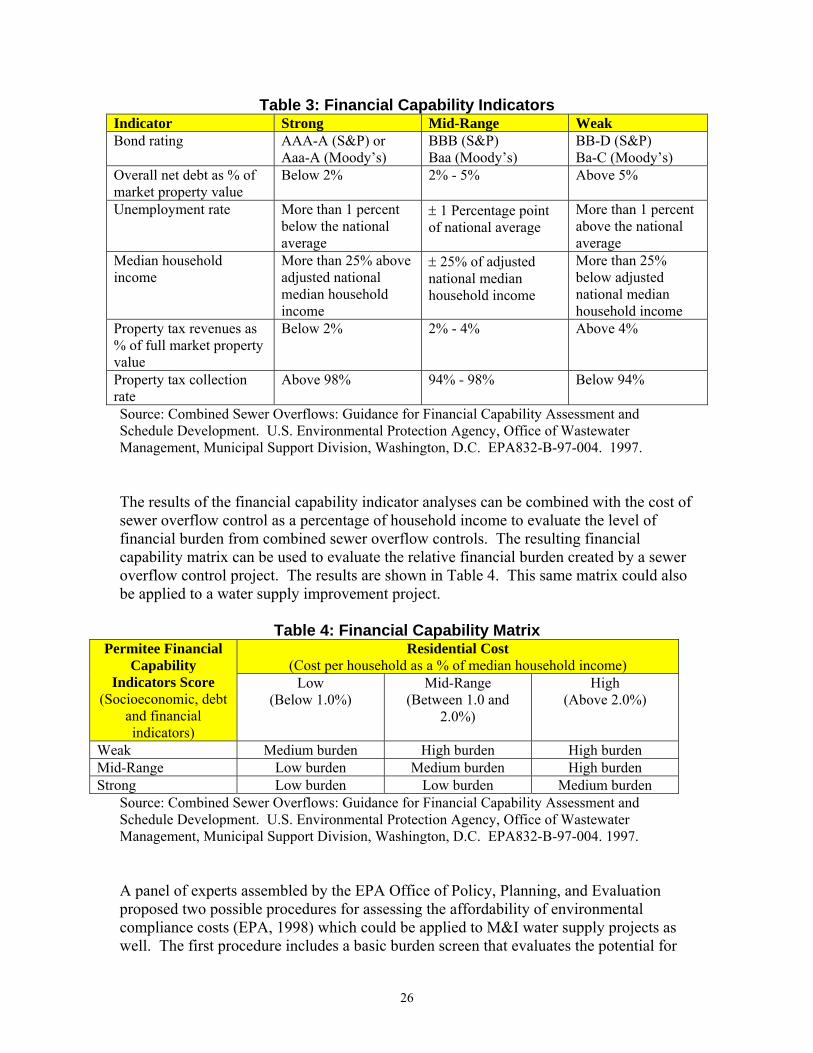
26

Table 3: Financial Capability Indicators Indicator Strong Mid-Range Weak Bond rating AAA-A (S&P) or

Aaa-A (Moody’s) BBB (S&P) Baa (Moody’s)

BB-D (S&P) Ba-C (Moody’s)

Overall net debt as % of market property value

Below 2% 2% - 5% Above 5%

Unemployment rate More than 1 percent below the national average

± 1 Percentage point of national average

More than 1 percent above the national average

Median household income

More than 25% above adjusted national median household income

± 25% of adjusted national median household income

More than 25% below adjusted national median household income

Property tax revenues as % of full market property value

Below 2% 2% - 4% Above 4%

Property tax collection rate

Above 98% 94% - 98% Below 94%

Source: Combined Sewer Overflows: Guidance for Financial Capability Assessment and Schedule Development. U.S. Environmental Protection Agency, Office of Wastewater Management, Municipal Support Division, Washington, D.C. EPA832-B-97-004. 1997. The results of the financial capability indicator analyses can be combined with the cost of sewer overflow control as a percentage of household income to evaluate the level of financial burden from combined sewer overflow controls. The resulting financial capability matrix can be used to evaluate the relative financial burden created by a sewer overflow control project. The results are shown in Table 4. This same matrix could also be applied to a water supply improvement project.

Table 4: Financial Capability Matrix Permitee Financial

Capability Indicators Score

(Socioeconomic, debt and financial indicators)

Residential Cost (Cost per household as a % of median household income)

Low (Below 1.0%)

Mid-Range (Between 1.0 and

2.0%)

High (Above 2.0%)

Weak Medium burden High burden High burden Mid-Range Low burden Medium burden High burden Strong Low burden Low burden Medium burden

Source: Combined Sewer Overflows: Guidance for Financial Capability Assessment and Schedule Development. U.S. Environmental Protection Agency, Office of Wastewater Management, Municipal Support Division, Washington, D.C. EPA832-B-97-004. 1997. A panel of experts assembled by the EPA Office of Policy, Planning, and Evaluation proposed two possible procedures for assessing the affordability of environmental compliance costs (EPA, 1998) which could be applied to M&I water supply projects as well. The first procedure includes a basic burden screen that evaluates the potential for

27

project costs to exceed ability to pay followed by a more rigorous secondary screen. The basic burden screen is based on the incremental cost per household of the proposed action and dividing the cost by median household income. Household income could also be measured in some other fashion, such as the mean or the mode. The result is then compared to other regions to determine if the cost is potentially too high. The secondary screen is performed for communities that appear to have a potentially high burden. The secondary screen would then look at the need for capital improvements in the study area (other than the project under consideration), access to various sources of financing, and eligibility for state and/or federal assistance. A second procedure proposed by the panel of experts emphasized the rationale for financial relief to communities considering an improvement. The basic burden screen in the second model would be used to determine if the residents of the jurisdiction would be unfairly burdened (that is, would annual costs be greater than some threshold level of income). If there would be an unfair burden, then the second stage would be a petition for relief. If the primary criterion for relief is not met, then the municipality could petition for relief based on the fact that the municipality is unable to finance the project at a reasonable cost. Relief could also be based on the fact that the cost of meeting mandated standards is excessively large relative to the level of resources in the municipality. The 1998 EPA analysis also presented a general framework for household affordability. This framework emphasized the impact of water charges on the ability of water users to support the full cost of water service through user charges and the percentage rate increase represented by the water supply change (rate shock). Affordability is greatly influenced by the ability of the water supply entity to secure financing and the financial resources of the water users. Several indicators of financial capability were identified. These indicators include: • financial structure and stability of the water system, including internal sources of

capital and business planning capability, • ratio of revenues to expenditures, • ratio of net income to revenues, • ratio of assets to liabilities, • debt-service coverage, • composite indicators of overall financial health in the region, • access to private and public capital. Indicators of overall financial health in a region can be evaluated in terms of the condition of local government finances, competing demands for capital, and operating expenditures. Other factors include debt as a percentage of market property value, tax revenues as a percentage of market property values, property tax collection or delinquency rates, and local expenditures per resident. General socio-economic indicators discussed previously can also be evaluated.

28

Access to private capital can be measured in terms of the ability of the water system to arrange financing through private sector equity and debt markets, credit and bond ratings, debt, and debt capacity. Bond ratings are an indication of the community’s credit capacity. General obligation bond (issued by a local government and repaid with taxes) ratings are an indication of the financial and socioeconomic conditions for the community as a whole. Revenue bonds are repaid with revenues from user fees, and indicate the economic conditions applicable to water users. Factors influencing availability of public capital include the ability of the water system to secure financing (grants or loan) from local or non-local public sources, credit and bond ratings, applicable priority rankings, and eligibility tests. The EPA is considering revising the methodology used to evaluate the affordability of implementing water treatment technologies to protect public health. Four areas of concern have been identified: 1) EPA’s approach to determining affordability for small systems, 2) components of the affordability determination method, 3) source water and regional disparities, and 4) whether financial assistance should be considered in EPA’s national-level affordability methodology (Federal Register, 2006). Recommendations have been sought from the EPA Science Advisory Board (SAB) and the National Drinking Water Advisory Committee (NDWAC) for revising the national-level affordability methodology. The SAB found that EPA’s approach for determining affordability for small systems addressed equity, efficiency, and administrative practicality considerations. However, the SAB recommended some changes to the 2 ½% of median household income threshold. A major concern was the fact that median household income does not reflect income inequality within water systems and may overstate affordability for low income households. Possible adjustments include using a lower income percentile within water systems (such as the 10th or 25th percentile rather than the median 50th percentile), considering whether a significant percentage of systems fall below the threshold even if the median does not, or the use of statistical measures of dispersion (variance or standard deviation) in addition to the mean to evaluate the number of households that may be excessively burdened. The SAB expressed concern that the 2.5% threshold may actually be too high when applied to smaller rural systems with lower incomes. The use of current water bills as the baseline from which regulations are considered affordable may not be a true measure of discretionary income available. Affordability should be evaluated as the incremental change in costs as a percentage of income. The NDWAC considered the same issues and came up with slightly different recommendations. First, the NDWAC believed the use of median household income as a measure of financial resources was appropriate. Second, the NDWAC felt the approach using 2.5% of median household income should be replaced with an incremental approach, where the cost associated with each new treatment rule should be compared to household income. The calculated percentage would then be compared to an affordability standard. This standard could be based on willingness to pay, defensive measures that would be needed to avoid a water supply problem, or a more arbitrary measure such as “doubling of current water bills.” The NDWAC did not believe the

29

affordability threshold should be more than twice the amount of current water bills. Since the average water bill is currently 0.5 to 0.6 percent of median household income, one percent of MHI was recommended as the incremental affordability threshold. Last, the NDWAC believed that when data are available, regional criteria should be developed for urban and rural distinctions. Water Supply Affordability Measures from Other Agencies The majority of affordability guidelines for water and sewer services have been produced by EPA. However, other agencies and consumer groups involved in various aspects of providing water supplies and treatment have produced affordability guidelines as well. The Department of Housing and Urban Development has set an affordability threshold of 1.3% of household income for water payments and 1.4% for sewer payments (EPA, 2006). A study by the National Consumer Law Center independently set affordability thresholds for water bills and sewer bills at 2.0% of average household income for each service, which corresponded with the EPA guidelines (National Consumer Law Center, 1991). United States Department of Agriculture Rural Development grant eligibility criterion uses a threshold debt service portion of annual user charge of greater than 0.5% of income when income is below 80% of the state median household income (EPA, 2006). The Rural Development threshold for the debt service portion of annual user charge is greater than 1.0% of income when income is between 80% and 100% of the state median household income (EPA, 2006). Payment Capability/Affordability Based on a Household Budgeting Approach The EPA and other agency affordability thresholds discussed above are based on a variety of factors including financing considerations, current rates, household income, and costs of alternate water supplies. It is recognized that the thresholds do not generally represent a maximum payment that can be made for water supplies. The actual ability of water users to pay for water supplies can be defined as the maximum amount households could pay for water given their income after accounting for housing expenses, transportation costs, food costs, insurance payments, other necessary expenses, and some level of discretionary spending. However, it would be very difficult to account for all possible household expenses to derive residual income that would potentially be available for making water payments. For example, what would be considered a necessary level of saving for an average household? The proportion of income that households could pay for water service will vary considerably from region to region. In regions with low housing costs, the percentage of income that could be used for water bills will be greater than in areas with high housing costs all else equal. Households in areas that have very poor water quality or service may be willing to give up some goods and services and use those funds for higher water costs.

30

A 1999 study assessing the financial and economic feasibility of rural water system improvements provides a framework for using a simple household budgeting methodology to estimate the ability to pay of water users for water supply improvements (Piper and Martin, 1999). This methodology accounts for necessary household expenses, differences in household income, and assumes that the highest observed water payments as a percentage of income made by households in a specific region represent an upper limit of ability to pay. The study identified a five step procedure that could be followed to estimate household payment capability. Step 1: Gather water cost information for water users outside the area being evaluated. Step 2: Collect household income, housing cost, tax payment, utility cost, insurance

payment, and other necessary expense data for households outside the study area but in the same general region.

Step 3: Calculate residual household income (income less payments for housing, taxes, utilities other than water, etc.).

Step 4: Calculate the cost paid for water per $1,000 of residual income by water users outside the study area but in the same region (ability to pay factor).

Step 5: Apply the ability to pay factors to the residual income of households in the study area. The factors applied could be the highest factor observed from the data, the factor that separates the top 10% of factors from the other 90% of factors, median factor, or some other factor that represents maximum ability to pay.

The ability-to-pay factors represent the proportion of discretionary income that households served by various utilities must spend for domestic water supplies. Therefore, they are a measure of dollars spent on water service per dollar of discretionary household income. The ability-to-pay factors represent actual payments made by households for water. Therefore, the higher factors are likely to be the best estimate of maximum ability to pay. This methodology provides an estimate of ability to pay that accounts for variation in household income, household expenses, and costs of living that are not considered when using set percentages of household income. Accounting for the variation in the percentage of total income spent by different levels of income may better represent household ability to pay for water supplies. Payment Capability/Affordability For Commercial and Industrial Water Users The payment capability/affordability evaluation approaches discussed above deal with residential water users. However, in many cases commercial and industrial water users represent a significant percentage of water use and a potentially large source of funding for water supply projects. Ignoring commercial and industrial payment capability may significantly understate the financial resources available to pay for water supply improvements.

31

One option that could be used to estimate the payment capability of commercial and industrial water users is to apply the 2.5% payment threshold for households to the value of receipts for commercial enterprises. However, due to the diversity in the types of commercial enterprises that may exist in a region and the very different cost structures that exist for different types of businesses, measuring payment capability in terms of a percentage of sales receipts is not likely to be a reliable measure of affordability. Another option is to estimate the funds available from commercial establishments to pay for water supplies using a procedure similar to the household budgeting approach for residential water users. Gross revenues for representative commercial establishments in the study area could be obtained from available data (the geographic area depends on the source of data) and necessary expenses are subtracted from revenues to estimate the maximum financial resources available for water payments. Necessary expenses include all payments for labor, capital, overhead, principal and interest payments, a reasonable rate of return on investment or return as a percentage of gross revenues, and any other expenses required to operate a business. The resulting net revenue represents an amount that could be paid towards water payments. If the result is zero or negative, then the amount that could be paid by commercial establishments is zero. The U.S. Bureau of the Census Economic Census and the Annual Survey of Manufactures are two potential sources of cost and expenditure data for commercial establishments from which generic estimates of the percentage of net revenues available for water supply payments can be estimated. The latest 2007 Economic Census data can be obtained at the website www.census.gov/econ/census07 and the Annual Survey of Manufactures can be obtained at www.factfinder.census.gov. Office of Management and Budget Circular A-94, “Guidelines and Discount Rates for Benefit-Cost Analysis of Federal Programs, “ indicated that a marginal pretax rate of return on an average investment in the private sector was approximately 7 percent for 1992. Appendix C to OMB Circular A-94 is periodically updated to reflect most recent economic conditions. The December 2009 Appendix C revision for nominal interest rates on U.S. Treasury notes and bonds from 3 years to 30 years ranged from 2.3% to 4.5%. This range could be used as a reasonable rate of return for a general case and more site specific and industry specific rates could be used when data are available. The budgeting approach discussed above can be used to estimate a representative percentage of gross business revenues that could potentially spent for water by a business that fits into a particular business category or general business sector. However, due to the aggregated nature of the data, the resulting percentages can only be considered an approximation of the payment capability/affordability of a specific commercial establishment. Adjustments may need to be made for specific circumstances in a study area which may require information from individual commercial establishments.

32

Other Considerations and Issues Another important issue that should be considered when planning an M&I project is how project costs should be allocated among the water users. Economic theory suggests that those who get the greatest benefit should pay the greatest cost. However, applying the principle of ability to pay suggests that those who can pay the greatest amount should pay the largest amount, as long as the overall project benefits are greater than the costs. Economic theory also indicates water users should pay the marginal (or incremental) cost of providing water to that particular group of users. Therefore, based on the marginal cost principle, the additional cost of expanding a water supply to serve a new group of water users or to improve water quality for existing users should be paid entirely by the affected water users. Applying the marginal cost principle would require a community of water users to pay the full cost of facilities which solely serve that community plus any incremental costs of shared facilities that are attributable to that community. The incremental shared facility cost paid by each community could be based on the proportion of total water delivered to each community using those shared facilities. Applying these principles may be very difficult for practical and/or political reasons. The cost of shared facilities could also be allocated equally among all users and added to facility costs that are attributable to a given community. Another possibility for allocating costs could be to simply calculate the average cost per unit of water delivered and multiply that by the units of water delivered to each user. This is an equitable method for allocating costs, but would not accurately reflect the facility costs attributable to each water user. However, there are many variations in project characteristics that can complicate the decision on how to divide project costs among water users. What if the system expansion provides improvements in reliability or water quality that benefits existing water users? In this case should existing water users pay some of the costs of expansion and if so, how much? Another possibility is that expanding a water system lowers per unit water costs due to economies of scale. In this case expanding to include a group of new users provides a financial benefit to all users. This scenario can also be applied to planning a new regional water system, where including a relatively low cost densely spaced group of users will lower the average cost per user compared to a system which does not include the low cost group. So, should a lower water rate be offered to the low cost group (based on a lower marginal cost)? If a high cost group of users want to be included in a project, should they be given a high rate based on the high marginal cost? On the other hand, perhaps the high cost group of water users should be subsidized by other users that have a high payment capability to include as many water users as possible in a new high quality water supply system.

33

Another complication occurs when a relatively large group of water users can benefit from construction of a large regional water system. For example, suppose that a proposed water system will include rural areas, small towns, and larger municipalities. Also assume that one of the large municipalities has excess payment capability (payment capability that exceeds their share of costs, regardless of how the costs are determined). If the large municipality sees great benefit to building the water supply project, then the large municipality may be willing to pay more than their proportionate share of project costs. This benefit may be the result of a need for water supplies due to water quality or reliability problems or future growth but the lack of any other alternatives that could provide these supplies. The cost savings per unit of water supplied may be so large that the cost savings from the regional project is greater than the cost of a smaller project serving one municipality. In order to ensure that the project is built, the large municipalities may be willing to subsidize some of the costs to the smaller towns and rural areas that don't have sufficient payment capability. If there is a willingness of some towns with excess payment capability to "subsidize" areas for which the project is not financially feasible, then evaluating payment capability on a regional basis makes sense. It should be noted that household level affordability criteria are typically not used when determining a system's overall financial condition and credit capacity. Rate assessments are frequently completed to determine if rates for a system are low or high compared to other systems in a region. Very low current rates may constrain asset maintenance and very high rates may limit potential expansion of the industrial customer base. Rate assessments can be used to help document appropriate capital improvement plans and rates that reflect the full cost of service. Additional factors included in these plans and assessments include the diversity and size of a system's customer base, the strength of the local economy, the system's organizational structure and strength of management, and its liquidity (Francoeur, et. al, 1999).

Conclusion The primary goal of expanding the capacity or improving the reliability of an M&I water system is to meet water needs and as a result generate positive net benefits to water users and to society as a whole. In order to evaluate the desirability of an M&I project, theoretically correct methods of evaluating benefits and costs must be used. Construction related costs of an M&I water supply project are relatively easy to estimate based on engineering cost estimates. However, the benefits of an M&I project are much more difficult to estimate. Several different methods have been described in this paper which can be used to estimate M&I benefits. The type of analysis needed to correctly evaluate an M&I project depends on the situation in which the project is deemed necessary. An analysis of economic feasibility is used to determine if we are better off as a society with a project or without a project under consideration. If there are several alternatives that generate positive net benefits, a benefit-cost analysis can determine which project

34

generates the greatest net benefit. A project that is economically feasible indicates there is an improvement in economic welfare with the project in place so the project should be completed. Assuming that a project or action is legislatively mandated or is economically feasible, then an analysis of the payment capability of water users can be completed to evaluate the financial feasibility of the project. If the water users have the financial resources to pay for the project, then it is financially feasible. If payment capability is less than the project costs, then other financial resources must be found in order to make the project financially feasible. As long as a project is economically feasible (benefits greater than costs), it makes economic sense to provide federal, state, or local cost sharing in order to complete the project if the project is not financially feasible.

35

References

Abdalla, C.W. “Measuring Economic Losses From Ground Water Contamination: An Investigation of Household Avoidance Costs.” Water Resources Bulletin. Vol. 26, No. 3, 1990. Agthe, Donald E. and R. Bruce Billings. “Dynamic Models of Residential Water Demand,” Water Resources Research, Vol. 16, No. 3, 1980. Agthe, Donald E., R. Bruce Billings, John L. Dobra, Kambiz Raffiee. “A Simultaneous Equation Demand Model for Block Rates,” Water Resources Research, Vol. 22, No. 1, 1986. American Water Works Association. “Dawn of the Replacement Era: Reinvesting in Drinking Water Infrastructure. An Analysis of Twenty Utilities’ Needs for Repair and Replacement of Drinking Water Infrastructure.” A study sponsored by the AWWA Water Industry Technical Action Fund. Denver, CO. May 2001. Bergstrom, J.C. and P. DeCivita. “Status of Benefits Transfer in the United States and Canada: A Review.” Canadian Journal of Agricultural Economics. Vol. 47, No. 1, 1999. Billings, R.B. and W. Mark Day. “Demand Management Factors in Residential Water Use: The Southern Arizona Experience,” Journal of the American Water Works Association, Vol. 81, No. 3, 1989. Brookshire, D.S. and M. McKee. “Is the Glass Half Empty, Is the Glass Half Full? Compensable Damages and the Contingent Valuation Method.” Natural Resources Journal. Vol. 34, No. 1, 1994. Collins, A.R. and S. Steinback. "Rural Household Response to Water Contamination in West Virginia." Water Resources Bulletin. Vol. 29, No. 2, 1993. Congressional Budget Office. “Future Investment in Drinking Water and Wastewater Infrastructure.” Washington, D.C. November 2002. Dahl, D.S. 1992. “Poll respondents voice concern’s over region’s water quality and quantity.” Fedgazette. Federal Reserve Bank of Minneapolis, April 1992. Espey, M.J., J. Espey, and W.D. Shaw. “Price elasticity of residential demand for water: A meta analysis.” Water Resources Research, Vol. 33, No. 6, 1997. Foster, Henry S. and Bruce R. Beattie. “Urban Residential Demand for Water in the United States.” Land Economics, Vol. 55, No. 1, 1979.

36

Francoeur, Mary; Chee Mee Hu, and Thomas Paolicelli, Rating Methodology: Analytical Framework for Water and Sewer System Ratings, Moody's Investor Service, Municipal Credit Research, August 1999. Gottlieb, Manual. “Urban Domestic Demand For Water: A Kansas Case Study,” Land Economics, Vol. 39, No. 2, 1963. Howe, Charles W. and F.P. Linaweaver, Jr. “The Impact of Price on Residential Water Demand and It’s Relation to System Design and Price Structure.” Water Resources Research, Vol. 3, No. 1, 1967. Howe, C.W. and M.G. Smith. "The Value of Water Supply Reliability in Urban Water Systems." Journal of Environmental Economics and Management, Vol. 26, No. 1, 1994. Intarapapong, W., D. Hite, A. Jaafar, and D. Hudson. “Predicted vs. Estimated Welfare Measures: A Test of the Benefits Transfer Method.” Selected Paper, AAEA Annual Meeting, Tampa, FL. July 30-Aug, 2, 2000. Jones, C. Vaughan and John R. Morris. “Instrumental Price Estimates and Residential Water Demand,” Water Resources Research, Vol. 20, No. 2, 1984. Jordan, J.L. and A.H. Elnagheeb. “Willingness to Pay for Improvements in Drinking Water Quality.” Water Resources Research. Vol. 29, No. 2, 1993. Kirchhoff, S., B.G. Colby, and J.T. LaFrance. “Evaluating the Performance of Benefit Transfer: An Empirical Inquiry” Journal of Environmental Economics and Management. Vol. 33, No. 1, 1997. Laughland, A.S., L.M. Musser, W.N. Musser, and http://www.awra.org/jawra/authors/author_ShortleJamesS.html. “The Opportunity Cost of Time and Averting Expenditures for Safe Drinking Water.” Water Resources Bulletin. http://www.awra.org/jawra/toc/toc_29_2.html. Martin, Randolph C. and Ronald P. Wilder. “Residential Demand for Water and the Pricing of Municipal Water Services,” Public Finance Quarterly, Vol. 20, No. 1, 1992. National Consumer Law Center. "The Poor and the Elderly - Drowning in the High Cost of Water.” Special report, 1991. Boston, MA. Nieswiadomy, Michael L. and David J. Molina. “Comparing Residential Water Demand Estimates under Decreasing and Increasing Block Rates using Household Data,” Land Economics, Vol. 65, No. 3, 1989. Nieswiadomy, Michael L. “Estimating Urban Residential Water Demand: Effects of Price Structure, Conservation, and Education.” Water Resources Research, Vol. 28, No. 3, 1992.

37

Nieswiadomy, Michael and Steven L. Cobb. “Impact of Pricing Structure Selectivity on Urban Water Demand,” Contemporary Policy Issues, Vol. 11, 1993. Pearce, D.W. (Ed.). The MIT dictionary of modern economics. 4th edition. MIT Press. Cambridge, MA. 1994. Piper, S. and W.E. Martin. “Household willingness to pay for improved rural water supplies: A comparison of four sites.” Water Resources Research. Vol. 33, No. 9, 1997. Piper, S. “Using Contingent Valuation and Benefit Transfer To Evaluate Water Supply Improvement Benefits” Journal of the American Water Resources Association. Vol. 34, No. 2, 1998. Piper, S. and W.E. Martin. “Evaluating the Accuracy of the Benefit Transfer Method: A Rural Water Supply Application in the USA.” Journal of Environmental Management. Vol. 63, 2001. Piper, Steven. “Impact of Water Quality on Municipal Water Price and Residential Water Demand and Implications for Water Supply Benefits.” Water Resources Research, Vol. 39, No. 5, 2003. Powell, J. and D. Allee. “Willingness to Pay for Protection of Water Supplies in Massachusetts Towns.” International and Transboundary Water Resources Issues. American Water Resources Association, Herndon, VA, 1990. Renwick, Mary, Richard Green, and Chester McCorkle. “Measuring the Price Responsiveness of Residential Water Demand in California’s Urban Areas.” A report prepared for the California Department of Water Resources, Sacramento, CA. May 1998. Renwick, Mary E. and Sandra O. Archibald. “Demand Side Management Policies for Residential Water Use: Who Bears the Conservation Burden?” Land Economics, Vol. 74, No. 3, 1998. Saunders, Margot. "Water and Sewer Rates--The Emerging Crisis for the Poor." In Proceedings of the Biennial Regulatory Information Conference. Columbus, OH: The National Regulatory Research Institute. 1992. Schneider, Michael L. and E. Earl Whitlach. “User-Specific Water Demand Elasticities.” Journal of Water Resources Planning and Management. Vol. 117, No. 1, 1991. Schultz, S.D. and B.E. Lindsay. “The Willingness to Pay for Groundwater Protection.” Water Resources Research. Vol. 26, No. 9, 1990. United States Environmental Protection Agency. “Water Utility Financing Study.” Office of Drinking Water, Washington, D.C. 1980.

38

U.S. Environmental Protection Agency. Municipality's Ability to Pay (MABEL): Volume 1 - User's Manual. Office of Policy, Planning, and Evaluation, U.S. Environmental Protection Agency, Washington, DC. June 1990. U.S. Environmental Protection Agency. ABEL User's Manual. Office of Enforcement, Washington, DC, October 1991. U.S. Environmental Protection Agency. The Road to Financing: Assessing and Improving Your Community's Credit. Office of Water, Washington, DC. EPA 832-B-92-004. October 1991. U.S. Environmental Protection Agency. Guidance for Calculating Municipal and Not-for-Profit Organizations' Ability to Pay Civil Penalties Using Current Fund Balances. Toxics Enforcement Policy Branch, Office of Compliance Monitoring, Washington, DC. March 1993. U.S. Environmental Protection Agency. Affordability of the 1986 SDWA Amendments to Community Water Systems. Prepared by ICF, Inc., Drinking Water Standards Division, Washington, DC. September 30, 1993. U.S. Environmental Protection Agency. Combined Sewer Overflow Financial Capability Assessment Guidebook. Office of Drinking Water, Washington, DC. September 1993. U.S. Environmental Protection Agency. Development and Analysis of Community Financial Profiles. Drinking Water Standards Division, Office of Ground Water and Drinking Water, Washington, DC. September 1993. U.S. Environmental Protection Agency. Economic Guidance for Water Quality Standards: Workbook. Economics and Statistical Analysis Branch, Office of Science and Technology, Office of Water, Washington, DC. November 1993. U.S. Environmental Protection Agency. Evaluating Municipal Environmental Burdens. Prepared by The Cadmus Group, Inc. Office of Policy, Planning, and Evaluation, Washington, DC. September 30, 1994. U.S. Environmental Protection Agency. Proceedings of the Blue ribbon Panel on Safe Drinking Water Act Costing. Office of Drinking Water, Washington, DC. October 1996. U.S. Environmental Protection Agency. Combined Sewer Overflows: Guidance for Financial Capability Assessment and Schedule Development. Office of Wastewater Management, Municipal Support Division, Washington, D.C. EPA832-B-97-004. March 1997. U.S. Environmental Protection Agency. Information for States on Developing Affordability Criteria for Drinking Water. Office of Water, Washington, D.C. Report EPA 816-R-98-002. Feb. 1998.

39

U.S. Environmental Protection Agency. “Information for States on Developing Affordability Criteria for Drinking Water. Appendix E. Affordability Measures and Thresholds: Selected Studies.” Located at website http://www.epa.gov/docs/ogwdw000/smallsys/affapp-e.html. Last accessed Dec. 7, 2006. U.S. Office of the Federal Register. “Small Drinking Water Systems Variances – Revision of Existing National Level Affordability Methodology and Methodology To Identify Variance Technologies That are Protective of Public Health,” 71 Federal Register 41 (2 March 2006) pp. 10671 – 10685. U.S. Water Resources Council. Economic and Environmental Principles and Guidelines for Water and Related Land Resources Implementation Studies. Government Printing Office, Washington, DC. 1983. Weber, Jack A. “Forecasting Demand and Measuring Price Elasticity,” Journal of the American Water Works Association, Vol. 81, No. 5, 1989. Williams, Martin. “Estimating Urban Residential Demand for Water Under Alternative Price Measures,” Journal of Urban Economics, Vol. 18, 1985. Williams, Martin and Byung Suh. “The Demand for Urban Water by Customer Class,” Applied Economics, Vol. 18, 1986. Wong, S.T. “A Model on Municipal Water Demand: A Case Study of Northeastern Illinois.” Land Economics, Vol. 48, No. 1, 1972. Young, Robert A. “Price Elasticity of Demand for Municipal Water: A Case Study of Tucson, Arizona,” Water Resources Research, Vol. 9, No. 4, 1973.