KSD-TR-7

ESD RECORD COPY RETURN TO

CAL INFORMATION DIVISION

210

ESD ACCESSION LIST TRl Call No. lizJ^L

^cys. Copy No.

Technical Note 1972-19

Description of the Lincoln Laboratory Wideband ELF Noise Recording Systems

J. E. Evans D. K. Willim J. R. Brown

14 April 1972

pared for the Department of th<- N under FUrctronir Systems Division Contract Fl%28-70-C-0230 by

Lincoln Laboratory MASSACHUSETTS INSTITUTE OF TECHNOLOGY s inpton, Massachusetts -

ADlHdooo

Approved for public release; distribution unlimited.

MASSACHUSETTS INSTITUTE OF TECHNOLOGY

LINCOLN LABORATORY

DESCRIPTION OF THE LINCOLN LABORATORY WIDEBAND

ELF NOISE RECORDING SYSTEMS

/. E. EVANS

Group 44

D. K. WILLIM

Group 66

J. R. BROWN

Group 25

TECHNICAL NOTE 1972-19

14 APRIL 1972

Approved for public release; distribution unlimited.

LEXINGTON MASSACHUSETTS

The work reported in this document was performed at Lincoln Laboratory, a center for research operated by Massachusetts Institute of Technology. The work was sponsored by the Department of the Navy under Air Force Contract F19628-70-C-0230.

This report may be reproduced to satisfy needs of U.S. Government agencies.

ll

ABSTRACT

This report describes the systems used to record wideband (12 Hz -

300 Hz) extremely low frequency (ELF) electromagnetic noise in a number of

geographic locations. The first section centers on the analog recording

system employed in Florida. Simply stated, analog tapes were recorded

and later converted to digital tapes for further processing. Section II des-

cribes the "NAVCOM" system which employed on site digital recording. The

final section describes the calibration procedures used to relate the

digitalized data to absolute electromagnetic field levels.

A distinctive feature of both systems is the care taken to preserve

the wide dynamic range of the ELF noise while reducing the amount of man-

made interference recorded. Results of analyzing the recorded noise data

to optimize communications system performance in this frequency band are

described in companion reports.

Accepted for the Air Force Joseph R. Waterman, Lt. Col. , USAF Chief, Lincoln Laboratory Project Office

in

I. INTRODUCTION

A decision was reached by the Laboratory during the Fall of 1967

to enter a program to collect and analyze extremely low frequency (ELF)

electromagnetic atmospheric noise after it became apparent that previous

noise-measurement programs had concentrated on narrowband measurements

that might conceal properties of the noise which could be exploited in a

receiving system. The objective of the program was to record and analyze,

in as wide a band as practical, ELF noise from geographical locations with

low power-line interference and high thunderstorm activity.

A description of the recording effort is facilitated if it is undertaken

in three sections. The first section centers on the analog recording system

employed in Florida. Simply stated, analog tapes were recorded and later

converted to digital tapes for further processing. Section II describes the

"NAVCOM" system which employed on site digital recording. In both cases

the antennas and front ends are essentially identical. The final section

describes the calibration procedures used to relate the digitalized data to

absolute electromagnetic field levels. Some results of the analysis effort are

described in [4-6].

II. DESCRIPTION OF RECORDING SYSTEM AND DIGITAL TAPE FORMAT FOR "LASA" FORMAT DIGITAL TAPES (FLORIDA RECORDINGS)

The initial noise-measurement effort concentrated on the

design and procurement of equipment and the location of a suitable site. A

satisfactory site was located on property of the Lykes Brothers Steamship

Lines near LaBelle, Florida (26° 51'N, 81° 31'W). A preliminary field

survey showed that 60 Hz electromagnetic fields did not interfere. In

addition, the site was removed from all well traveled roads, thus eliminating

ground vibration as an interfering effect. The site is located in a region

where there is extremely high thunderstorm activity from June through

September.

A. Description of Antennas

Two loops and one whip antenna were constructed to measure

the horizontal magnetic and vertical electric fields. The loops are oriented

in a north-south, east-west configuration and are mounted inside a temporary

8- by 8- by 8-foot hut constructed of 3-inch Dyrelite foam laminated onto

0.25-inch plywood. Both loops are rigidly mounted onto a base which is then

physically isolated from ground motion by several layers of packing material.

Each of the loops is 1. 57 meters in diameter and contains 471 turns of No. 14

copper wire. The turns area product is 910 square meters. The low-

frequency series equivalent circuit of the loop is comprised of a 0. 75-henry

inductance in series with a 190 resistor. Self-resonant frequency of the

loops is approximately 6 kHz.

Electrical field strength is sensed by a 12-foot vertical whip antenna

enclosed in a 12-inch fiberglass cylindrical windshield. Guying is provided

for the windshield in the event of high winds, but it is otherwise self-

supporting. The whip antenna is located approximately 40 feet from the hut

enclosing the loops. A ground system is established with 12 bronze rods

driven 8 feet down and interconnected by 1-inch copper braid. Figure 1 shows

the site in May 1968.

B. Electronics Description

The initial measurements were accomplished with an analog

tape-recording system. This instrumentation was superseded by the digital

recording system described in the next section. The following description is

that of the analog recording system. Noise data was recorded in the FM mode

and returned to the Laboratory where digital tapes were made for detailed

digital processing. Since the only available tape recorders required 60 Hz

power for the tape drive, it was necessary to separate the recorder and the

sensitive antennas by 2 00 feet to reduce self-interference. The hut contains its

own batteries, preamplifiers, calibration circuits, and line drivers; a distant

vehicle contains line receivers, tape recorder, monitoring circuits, batteries,

and remote control of the hut electronics. A detailed block diagram of the

recording system is shown in Fig. 2.

1. Hut Electronics

Located in the hut are the three preamplifiers for the three

sensors. Each loop is coupled into its amplifier through a 50-to-l step-up

transformer. Loop amplifiers are the high-input impedance field effect

transistor (FET) type. These amplifiers have a gain of 20 dB and are

mechanically insulated from their surroundings to avoid microphonic effects

associated with such high-impedance devices. Input transformer characteris-

tics restrict the useful bandwidth to approximately 3 00 Hz. An additional

low-pass filter with cutoff at 320 Hz and a steep skirt follows each loop pre-

amplifier to further remove out-of-band noise. Tangential signal sensitivity

at 20 Hz for the loop channels is calculated as - 30 dB with respect to

1 ija/m/./Hz.

An FET high-input impedance source follower is utilized as an

impedance transformer for the whip channel. A voltage gain of 1. 0 is suitable

for this channel since voltage levels derived from the whip are higher and

dynamic range is extended if a lower gain is employed. The first field trip

revealed signal contamination due to wind movement of the whip and possible

"fair weather fields" that were unacceptable. A 12 Hz cutoff high-pass

filter was installed to diminish these effects. A 320 Hz low-pass filter also

serves to eliminate out-of-band interference and noise, including some VLF

stations.

The dynamic range of the atmospheric noise tends to be very large in

an area like Florida so some means are necessary to record the data without

compromising this range. In order to accommodate the 40 dB dynamic range

of the tape recorder a high and low gain version of each channel was recorded.

A 20 dB difference in gain was maintained between the two channels. Using

this method the recording process can be accomplished with a 60 dB range

of signal levels. Odd numbered channels were reserved for the low gain

version, even numbered channels are used for high gain recording. A limiter

clips the high noise peaks in the high gain channel prior to recording.

2. Remote Electronics

The actual recording process takes place in an air-

conditioned vehicle some 200 feet from the hut. Balanced line receivers

accept the six-channel information and apply it to six channels of the Ampex

FR 1300 tape recorder. A seventh recording channel is operated with zero

input for reasons to be discussed later. Tape speed is 15 inches/second

corresponding to a recording bandwidth of 5 kHz, and a record time of

approximately 40 minutes/reel. Some of the later tapes were made at

1 7/8 rps. Power for the tape recorder is derived from a DC-to-60 Hz

inverter contained in a doubly shielded magnetic enclosure. Operation of the

tape recorder does not introduce measurable additional 60 Hz components

in the recording process. An auxiliary edge track recording channel is

supplied to allow insertion of voiced comments including tape and time

identification. Monitoring of recorded signals is accomplished with an

oscilloscope and a channel-selector switch. All battery and supply voltages

are displayed on the monitor panel.

A rustrak strip chart recorder was also available to plot the average of

the mean square wideband signal. Averaging time was approximately 40

seconds for this recorder. Such a recording allows one to refer a particular

short-term tape to the general background intensity as measured over

several hours. It is particularly useful in establishing the rise and decline

of local thunderstorm activity.

C. Procedure

In making an analog tape, the following procedure is used:

(a) A voice entry is made identifying the day, time and

any important meterological phenomenon.

(b) One minute of the 30 Hz triangular wave calibration

is recorded.

(c) Six channels of data are recorded for approximately

37 minutes. During this time, local forecasts and weather conditions are

recorded from the AM radio in the vehicle as available. Any changes in local

weather conditions are also noted.

(d) One minute of the calibration signal is recorded at

the conclusion of the tape.

A simple direction of arrival unit has been constructed which operates

in conjunction with the two loops and one whip sensor to read out an x, y

plot on an oscilloscope. This unit has been used to verify the general location

of high-intensity storms and, on one occasion, the display was highly

correlated with a known storm center in the Fort Myers area.

D. Summary of Data Taken

Approximately 40 hours of analog recordings have been

obtained during several trips to the Florida site during 1968-69. All the 1968

data and part of the 1969 data has been converted to digital tapes. Data thus

far reveal the noise characteristics during a quiet period in February and a

moderately active period in May. In addition to the two Florida trips, one

investigatory trip was made to a remote area in New Hampshire to verify

that the general characteristics of noise measured at that site correspond to

that found in Flordia. Although the 60 Hz interference was high at this site,

it was possible to conclude that the noise at both sites was similar and,

furthermore, that there was nothing peculiarly different at either of the sites.

E. Analog-to-Digital Conversion

The analog tapes are returned to the Laboratory where

they are played back from an identical tape recorder at the record speed. At

this time, the output of channel 7 which does not contain data is subtracted

from the remaining six channels with the result that wow and flutter components

are diminished. The resultant signals are then applied to a multiplexer

which may be programmed to select from one to six channels for A/D con-

version via a 14-bit Adage model VMX-32B A/D converter and subsequent

digital recording. This digital tape is then the basis for further analysis.

The computer allows data analysis to take place with the full 60 dB dynamic

range.

In Figs. 3 and 4 we show the spectrum and amplitude probability

density function of the output of the A/D converter when the input terminals

were shorted. These two figures give a measure of the degradation in data

on the digital tapes due to jitter during the A/D conversion process.

Prior to A/D conversion, the playback electronics are adjusted so that

the 30 Hz triangular wave calibration had a 1. 0 volt peak-to-peak input level.

This enables one to check the digital tape produced to determine what

deviation, if any, exist between the actual ratio of digital levels/volt input

to the nominal level of 2144 digital levels/volt input.

F. Format of Converted Data on the Digital Tape

The output of the A/D converter is buffered onto a 7 track

800 bit per inch digital computer tape by a Digital Equipment PDP-7 computer.

The particular tape format used is an adaptation of a format used for

recording seismic array data on computer tape and has been given the name

"LASA" format tape for the purposes of this documentation. (References 1

and 2 give a description of the use of such tapes in the seismic work. ) The

converted data words are stored in the computer memory until 400 samples

from each channel have been converted whereupon a physical record consisting

of 4 header words together with the 400 samples from each channel are

written on the tape. To make the tape IBM compatible, the data is placed on

the tape in 6 bit blocks (with an odd parity bit in the seventh track ' ) and a

3/4 inch gap between physical records.

Any A/D conversions with a playback gain that deviates from this level have the playback level noted on the record of the particular A/D conversion.

Also, seven "longitudinal parity bits" are placed at the end of a physical record to further aid in error detection.

In Fig. 5, we show the relation of the 14 bit A/0 converter output to

the 18 bit data word put on the digital tape. The computer program (i. e. ,

read package "IOPAK") that reads the data from the digital tape into core

memory of the computer shifts the value on the tape right one bit so that the

least significant bit on the tape is lost (this was done to reduce effects of the

telephone line noise in the seismic program). Thus, the A/D converter

output is shifted left one bit before being recorded on the digital tape.

In Fig. 6 we show how the 18 bit words in the core memory of the

PDP-7 are placed onto the digital tape while in Fig. 7 we indicate the organiza-

tion of the header word information.

III. DESCRIPTION OF RECEIVER AND DIGITAL TAPES FOR "NAVY COMMUNICATIONS" FORMAT TAPES

The second generation recording systems used in the field* to

acquire broad band atmospheric noise data utilize digital tape-recording

techniques and, with the exception of the antennas and associated preamplifier

electronics are contained in mobile, self- supporting motor vehicle terminals.

A block diagram of one system is shown in Fig. 8. The following is a

description of this digital tape recording system which superseded the analog

system in September 1968.

Included in the first block to the left of the dashed line in Fig. 8 are

Ithaco preamplifiers, low-pass filters (320 Hz), and Burr-Brown line drivers

using a balanced input and output configuration. This portion of the system

is essentially the same as the front end of the analog system.

The conditioned signals from the dual loops and vertical whip antenna

are carried to their respective line receivers over approximately 200 feet

of twisted pair shielded balanced line. The 200 feet represents the separation

between the antenna location and the data-recording terminal. All equipment

to the right of the dashed line in Fig. 8 is found in the recording terminal,

and all to the left, with the exception of the whip antenna, is enclosed within a

To date, this system has been used successfully in Norway, Malta and Saipan.

prefabricated wooden shelter. The whip antenna is contained in a separate

cylindrical fiberglass enclosure to reduce wind loading. A full description

of the antenna configuration, both physical and electrical, was given in the

previous section.

Following the line receivers is a calibrate switching network where

calibration signals are injected in place of the antenna signals. The calibrate

switching is effected by means of an analog multiplexer utilizing high-speed

FET's.

The three outputs of the switching net are amplified and passed through

twin "T " active 400-cycle notch filters. System power is supplied at 28 and

12 volts DC. However, some of the equipment is standard off-the-shelf

hardware and was not designed around a DC power source. Therefore, DC

to 400-cycle AC solid-state inverters are used to supply the required 115-volt

AC primary voltage for those particular devices. The purpose of the

400-cycle notch filters is, of course, to eliminate any possible interference

from the 400-cycle inverters.

At the output of the notch filters, the three signals are divided into

two paths each, with more amplification in each leg to scale the signals up

in level for the ± 10 volt peak signal reference used in the following analog-

to-digital conversion process. One of the paths of each signal has an

additional 36 dB of gain represented by amplifiers G in Fig. 8. The function

of this additional amplification is to effect a better than 90 dB dynamic range

using only a single 12-bit analog-to-digital converter. The way in which this

is performed will be discussed later.

The resulting six signal paths, a high-and low-gain channel of each of

the three original signals, form the inputs to six sample-and-hold amplifiers.

The sample-and-holds are Raytheon models SH9 with aperature times in the

order of 50 nsec and settling times of 5 (jsec maximum. At this point, the

analog signals are simultaneously sampled at a 1 kHz rate and held as they

are sequentially multiplexed through to a 12-bit analog-to-digital converter.

The multiplexer and A/D converter combination is a Raytheon multiverter

package using a model ADC21-12B converter with 11 bits plus sign in 2's

complement code. Since the throughput rate of the multiverter is 50 kHz,

the analog signals are sampled and converted to digital form in 50 kHz bursts

at a burst rate of 1 kHz. Each burst is composed of six (12-bit) digital words,

with a high-and-low-order word describing samples of each of the three

original analog signals.

With 36 dB of additional gain in the low-order (high-gain) path of each

signal, the combination of the high-and low-order (12-bit) samples effect a

data sample word length of 18 bits. This may be more easily described by

referring to Fig. 9. For simplicity, two A/D converters are shown in the

figure, where in the actual system only one is time-shared in the multiverter.

The point labeled "analog data sample " is the point at which the signals are

divided into two paths each, with one path of each containing the additional

gain. Both samples are converted to 11 bits plus sign (sequentially through

the multiplexer by a single A/D converter in the actual system) and passed

onto the recording as two separate words.

During processing of the recorded tape on a computer, the programmer

may select which of the two words will be used as the data sample or, after

checking for correlation of the five overlapping bits, may use the combination

of both words for an effective 18-bit data word. The 17 bits of magnitude

represent a dynamic range of 102 dB, but discounting the first couple of bits

to system noise results in a more realistic figure of 15 bits of resolution for

a dynamic range of 90 dB.

It must be noted that the dynamic range figure given above assumes

that all recorded data is of equal interest. If, however, strong background

The algorithm used to date at Lincoln Laboratory has been to:

1. Set the data value = (low order data word - low order dc offset) if the low order data word absolute value is less than or equal to 1024 (= 2 10).

2. Otherwise, set the data value = (high order dataword - high order dc offset) x (ratio of high order gain/low order gain). The equipment is normally adjusted to produce a ratio of 64:1.

interference (e.g. , that caused by power lines) is present in the data the

useful data to noise ratio obtained with the above system may be well below

that obtained using an 18 bit A/D converter. This situation was observed

experimentally in recordings at a site in Malta where the very strong 50 Hz

radiation from a nearby power line caused the lower order data word to

saturate continually so that the high order data word was generally utilized.

The quantization noise of the high order data word has an rms value of 19

levels which was comparable to the natural EJLF noise levels. Thus, even (

though the 50 Hz power line could be removed from the digitized data by

appropriate digital filtering, the filtered data was not representative of

natural ELF noise due to the increased quantization noise. This particular

problem was solved by additional analog notch filtering prior to the A/D

converter.

Additional insight into the differences between the 18 bit data word

obtained by combining the two overlapping 12 bit data words and an 18 bit

data word obtained from an 18 bit A/D converter can be obtained from

Fig. 19. In Fig. 19, we have plotted the ratio, R, of signal level to rms

quantization noise as a function of signal level. We see that R is mono-

tonically increasing with signal level for an 18 bit A/D converter whereas

there is a drop in R for the ELF noise recording system when the low order

data word saturates. From Fig. 19, we see that it is important that the

useful signal level be no worse than Z0 dB below the recorded signal level

for recorded signal levels near 1000 digital levels.

At the output of the A/D converter the 12-bit words are split into six-

bit characters, odd parity is added, and the resulting 7-bit characters are

passed on by means of a digital multiplexer to a tape buffer/formater (core

memory). Parity is checked for correctness first at the output of the memory

as the characters are transferred to the tape recorder, and again by the

read-after-write electronics in the tape transport. Visual error indicators

are available for both check points.

10

The digital tape transport used for recording is a Potter model FT-152

designed for field recording work and powered from a 12-volt DC source.

Recording is on seven tracks at a density of 800 BPI in IBM format.

At the 1 kHz sample rate of the three inputs with two 12-bit words per

input, the data rate is 12,000 6-bit characters per second. Each data record

is one second long with each headed by four additional 12-bit header words

for a total of 12,008 characters per record. Allowing for the IBM-compatible,

3/4 inch, inter-record gaps, the data-recording rate is 12.63 kHz. With an

800-BPI density and 3/4-inch gaps, the tape speed is a conservative 15. 8 inches

per seond. The transport accommodates 10 l/2-inch reels containing

2400 feet of tape. Each tape therefore holds approximately 30 minutes of

recorded data.

The format of the record header information is as shown in Fig. 10.

With the data record lengths of one second each, the count described by

header word 4 indicates record count from tape start as well as elapsed time

(seconds in binary) after the initial start time of header words 1 and 2. All

header information with the exception of the record counter and the calibration

indicator bit (automatically set during calibration records) is initially set up

by thumbwheel switches and automatically inserted at the proper time to head

up each record. In Fig. 11, we show how the header words and data words

are organized on the digital tape.

Calibration signals are inserted at the calibrate switching point (Fig. 8).

Calibration takes place automatically at the beginning of, periodically during,

and near the end of each digital tape recording. The periods of calibration are

one record length (1 second) duration repeated every 7 minutes through-out

each tape recording. The period length and repetition rate is thumbwheel

selectable from the control panel. Manual calibration control is also available

for initial calibration prior to recording. This calibration is used to check

gain and any change in DC offset between the line receivers and the A/D

converter output and is not to be confused with the absolute field strength

11

calibration of section IV, which is performed bi-weekly by inserting a known

signal level in series with the antennas.

Various signals can be used for the digital calibration. The waveform

used with recorded tapes prior to January 23, 1969 was a series of step

inputs, the amplitudes of which exercised full scale of both the high and low

order legs of the A/D conversion and also intermediate levels to fall within

the 5 bit crossover area of the two words.

To eliminate DC offset drift problems and also to simplify system

alignment procedures, the DC coupling between the-analog front end and the

sample and hold input to the A/D converter was replaced with RC coupling

on 23 January 1969. The 400 Hz notch filters were also deleted from the

circuits at that time. Since that time, both recording systems have used a

40 Hz sine wave calibration signal for the recording calibration source. As

before, this cal signal is used only to check gain ratio between the high and

low channels and also aid in the detection of any existing offset at the A/D

output.

As mentioned earlier, all equipment shown to the right of the dashed

line in Fig. 8 is found in a recording terminal. The recording terminal in

this case is a Clark Cortez camper vehicle, one model of which is shown

in Fig. 12.

In Figs. 13-15 we show the results of some tests made to determine the

dynamic range of the recording system. Figure 13 shows the spectrum of the

NS loop for Malta tape AN 1-047 of 25 November 1968 when the antenna was

replaced by an . 8 henry choke. Figure 14 shows the spectrum of the EW

loop for Malta tape AN 1-047 when the input to the EW loop preamplifier was

shorted. Figure 15 shows the spectrum of the NS loop when the input to the

NS loop sample and hold amplifier for the NS loop. From Figs. 13-15, it

appears that the observed system noise is quite low relative to the few bits

hypothesized for the system noise, and thus, the system dynamic range is

above 90 dB.

L2

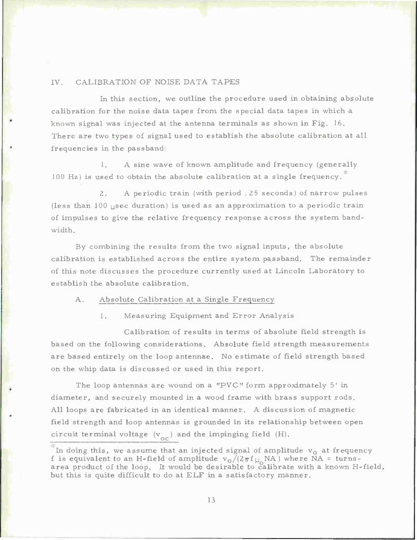
IV. CALIBRATION OF NOISE DATA TAPES

In this section, we outline the procedure used in obtaining absolute

calibration for the noise data tapes from the special data tapes in which a

known signal was injected at the antenna terminals as shown in Fig. 16.

There are two types of signal used to establish the absolute calibration at all

frequencies in the passband:

1. A sine wave of known amplitude and frequency (generally

100 Hz) is used to obtain the absolute calibration at a single frequency.

2. A periodic train (with period .25 seconds) of narrow pulses

(less than 100 (jsec duration) is used as an approximation to a periodic train

of impulses to give the relative frequency response across the system band-

width.

By combining the results from the two signal inputs, the absolute

calibration is established across the entire system passband. The remainder

of this note discusses the procedure currently used at Lincoln Laboratory to

establish the absolute calibration.

A. Absolute Calibration at a Single Frequency

1. Measuring Equipment and Error Analysis

Calibration of results in terms of absolute field strength is

based on the following considerations. Absolute field strength measurements

are based entirely on the loop antennae. No estimate of field strength based

on the whip data is discussed or used in this report.

The loop antennas are wound on a "PVC " form approximately 5' in

diameter, and securely mounted in a wood frame with brass support rods.

All loops are fabricated in an identical manner. A discussion of magnetic

field strength and loop antennas is grounded in its relationship between open

circuit terminal voltage (v ) and the impinging field (H).

In doing this, we assume that an injected signal of amplitude v0 at frequency f is equivalent to an H-field of amplitude w0/{Zffi \± NA ) where NA = turns- area product of the loop. It would be desirable to calibrate with a known H-field, but this is quite difficult to do at ELF in a satisfactory manner.

13

v = M HNA ca oc ^o _ n

p. = permeability of free space, 4TT x 10 henry/meter (used for air core antennas discussed here)

H s magnetic field, amps/meter 2

NA s turns area product of loop, (meters)

v = open circuit terminal voltage due to effect of H field averaged over area of loop, volts

co = (277-f) angular frequency of assumed sinusoidal field in radians/second.

Several questions related to the authenticity of loop measurements are

suggested by an examination of this formula.

(a) Turns Area (NA). Number of turns on the loop was

established with great care. Area was determined by direct measurement,

and verified by an independent experiment. Following the technique described

in [3] , a one turn loop, one meter in diameter was constructed. Utilizing

this loop as a transmitting antenna coaxial with the large receiving loop

excellent agreement with the predicted results were obtained. On the basis

this experiment and physical measurements the NA product is correct within

± 0.8$.

(b) Permeability (jj. ). Permeability of free space has

been assumed for the air core loops. During the experiment described above

measurements were conducted with and without mounting supports with no

noticeable effect. Placement of the front end electronics near the loop in the

normal mounting location produced no effect either. No error is assumed to

be present using the permeability of free space.

(c) Frequency. For calibration purposes it is necessary

to establish the calibration frequency with some accuracy. A HP 2 04C

oscillator was generally employed at the field sites to insert the calibration

signal at the antenna. Laboratory experiments reveal that the oscillator will

probably be set to an accuracy of ± 4$ at 100 Hz. Fortunately, this field

misalignment does not have to be tolerated as degrading the calibration since

14

the analysis programs can be used to ascertain the actual frequency employed

for a particular tape. Providing this method is employed no error need

accrue due to frequency mis-alignment. Frequency stability of this oscillator 4

(1 part in 10 per 20 minutes) is sufficient to impose narrow band filtering

(. 244 Hz) in the analysis program.

As stated before, the calibration signal is injected in series with the

loop antenna as shown in Fig. 16. In connection with this calibration method

several other factors will have a bearing on the resulting accuracy of the

calibration.

(a) A Ballantine Model No. 323 true rms voltmeter is

used to ascertain the signal level injected into the attenuator pad. If it is

assumed that the cal signal was measured at, or near full scale then the

result has an accuracy of ± 2$ at 100 Hz. If an average error in reading the

meter is assumed to be 1$ then the most probable error to be attributed to

the meter is ± 2.2$.

(b) The attenuator has been measured on a bridge and it

is accurate to ± 0. 1$.

(c) Wideband noise picked up by the antenna and coupled

back to the voltmeter is negligible.

(d) Atmospheric noise and possible power line harmonics

at or near the calibration frequency will affect the energy in the passband of

the analyzing filter used to "pick out" the calibration signal. This effect is

minimized by using a large calibration signal relative to the interference. A

signal to noise ratio of 40 dB in a 1 Hz bandwidth has been the typical ratio

in most of the calibration runs. Based on this ratio it is possible to say that

background noise has not affected the calibration signal estimate in any

significant manner.

(e) Gain stability and frequency response of the recording

system has remained relatively constant from calibration to calibration.

15

Maximum variation in gain has been 156 over a one month period.

(f) Quantization errors due to the 12 bit A/D converter

are insignificant at the signal levels used and no error is attributed to the

digital processing employed.

(g) Variation of sample rate is determined by the

stability of a temperature controlled crystal oscillator. Drift rate of this n

oscillator is one part in 10 /day. If the frequency drift is assumed monotonic

then the equivalent change in frequency at 100 Hz would be . 01 Hz after

1000 days. No error is associated with this source.

After consideration of the factors discussed here the following error

estimate is considered representative of the factors involved in the noise

measurement program.

Source Error

Turns area ± . 8$

Meter reading ± 2.2$

Attenuator pad ± 0. 1$

Gain variation ± 1.0

Peak error ± 4. 1 $ or ± .35 dB peak.

The most probable error assuming that the error from each source is

independent of the other and represents the 1Q level is

V (.8)2 + (2.2)2 + (. I)2 + (l)2 = 2.54$ or ± .22 dB.

2. Absolute Calibration at a Single Frequency from the Spectral Analysis Results for Sine Wave Calibration Tape

In this section, we discuss a method of determining the

absolute calibration at a single frequency from the results of spectrum analysis

using a spectral analysis computer program and the known amplitude of the

injected sine wave. The steps are as follows.

(a) Spectrum estimates are obtained every (1000/4096)Hz

16

from 1. 024 seconds of data. From the value of the spectrum at the frequency

of the injected sine wave, one can determine the amplitude of the sine wave

using formulas presented later on in this section.

(b) The recording site data log sheet that accompanies

the tape indicates the amplitude of the sine wave (generally in rms-volts)

injected at the antenna terminals.

(c) The H-field in amps per meter that is equivalent

to the injected signal is assumed to have amplitude

XT Voc 1.3918 x 10Z , -. . ,„ H = rr jr-zrr = ' > V (volts ) (1) 2frfNA f(Hz) oc y ' v

for the antennas with a turns-area produce NA = 910 square meters.

(d) From (a) and (c), we can establish the ratio between

(digital levels)2 and (amps/meter) at the frequency of the injected sinusoid

[one digital level = least significant bit in the high gain channel data word] .

We now want to determine the formula relating the amplitude in digital

levels to the value of the spectrum obtained by the spectral analysis computer

program. The method by which this computer program obtains spectra is

discussed in Ref. 4. We will consider here the case where the number of data

segments averaged over is one (the number of segments averaged over affects

the stability of estimates for noise data, but has no effect on the results for a

deterministic signal such as the sine wave used for calibration).

The computer program computes the estimate of the spectrum at

frequency f as:

s(fo> = 101°«10[SUMWT lX(fo»l2) <2)

where N-l -j2fff kT

X(fQ) T w(k)x(kT)e (3) k=0

N-l F

k=0 SUMWT = T w2(k) (4)

17

X(kT) = value of the input waveform at time kT

w(k) = data window used to reduce effects of power lines on the spectrum estimates

= 1 for all k if "no window" is used

= l _ |k"(*VZ) I if a »1 - |t | " window is used.

When the input is a sinusoid at frequency f with amplitude A, it can be

shown' that s(f ) is closely approximated by

s(fo) = 10 log10[j(N<w(k))A)2/N <w2(k)>] (5)

<wZ(k)>

where (w (k)) = time average value of [w(k)] . The quantity

^WW> = 1 for "no window" (7) (wZ(k))

= -| for "1 - |t| " window. (8)

Example

We now illustrate the above steps using data from Norway tape AN2-002.

The injected signal was of amplitude 25 mv rms into a 1000-1 pad (i.e. , the

value of resistance R in Fig. 16 was 1000 ohms) at a frequency of 1000 Hz.

In Fig. 17 we show the spectrum of the NS loop channel on this tape using

N = 1024 and a "1- |t | " data window. We now go through the steps of the

procedure outlined above:

(a) From Fig. 17, we see that the computed spectrum

level was approximately 93.97 dB at 100 Hz. Thus, from equations (6) and

(8), we conclude that the injected sinewave had an amplitude (peak) of

A = 3.622 x 103 digital levels.

By substituting x(kT) = A cos (27ff kT + 6 ) into equation (3).

(b) The injected signal at the terminals had an amplitude

(peak) of

v = (25 x 10"6 volts)(1. 414) = 35. 35 x 10~6 volts (peak).

(c) This is equivalent to a H-field of amplitude (peak)

H = 1,391S X 10 (35. 35 x 10"6) = 4.92 x 10"5 amps per meter. 1 x 1(T

(d) Thus, we conclude that at 100 Hz

- 8 1 digital level = 1.36 x 10 amps per meter.

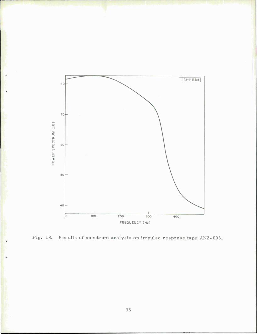
3. System Relative Frequency Response from the Spectrum Analysis Results for Impulse Train Calibration Tapes

The determination of the system relative frequency response

from spectrum analysis of a calibration tape generated by injected periodic

train of narrow pulses at the antenna terminal (as indicated in Fig. 16) is

quite straight-for ward. In Fig. 18, we show the results of such an analysis

(using N = 1024 samples of data and transforms of length 4096 samples) on

Norway tape AN2-003. It should be noted that the frequency response shown

in Fig. 18 does not include the antenna transfer function between H-field and

volts at the antenna terminal. This antenna transfer function (of 6 dB per

octave) must be included in determining the absolute calibration at all

frequencies from the single frequency calibration.

19

Fig. 1. Florida noise measurements site.

20

ro

Fig. 2. Detailed block diagram of noise instrumentation.

20 18-4-13375|

10

3 o

SP

EC

TR

UM

o

| -20 -1 2 J4 LJUJJJ 1 1 1 L II. h i. .

-30

-40 i i i 100 200 300

FREQUENCY (Hz)

400

Fig. 3. Spectrum of output of A/D converter with input shorted.

22

10" 18-4-13378

10

o

Ü

3 U. >■

UJ

Q

00 < CD

o CC Q-

10^

10"

RMS LEVEL = 3.96 DIGITAL LEVELS

MEAN = 4.4 DIGITAL LEVELS

-8 -6 -4-2 0 2

RMS UNITS FROM MEAN

Fig. 4. Probability density function of output of A/D converter with input shorted.

23

MSB

18-4-133 77

LSB

A/D CONVERTER OUTPUT s 1 2 3 4 5 6 7 8 9 io|n 12|l3

18 BIT COMPUTER WORD | s s s s 1 2 3 4 5 6 7 8 9 1011 12 13 X

EXTENDED SIGN BIT

ALL DATA RECORDED WITH ODD PARITY IN TWO'S COMPLEMENT FORM

14 BIT A/D VALUE IS SHIFTED LEFT ONE BIT BECAUSE READ PACKAGE "IOPAK" SHIFTS DATA VALUE FROM TAPE RIGHT ONE BIT THIS LAST BIT 15 MEANINGLESS.

Fig. 5. Relation of 14 bit A/D converter output to 18 bit data word for "LASA" format digital tapes.

24

18-4-13378

PDP-7 CORE MEMORY

0 1 2 3 4 5 6 7 8 9 10 11 12 13 14 15 16 17

1ST SAMPLE OF EACH CHANNEL

2ND SAMPLE OF EACH CHANNEL

HEADER WORD 1

CHANNEL 1

CHANNEL 3

HEADER WORD 1

f

Ul EADER WORDS

END OF RECORD

TAPE

0 1 2 6 7 8 12 13 14

3 4 5 9 10 11 15 16 17

0 1 2 6 7 8

12 1314

3 4 5 9 10 11

15 16 17

0 1 2 6 7 8 12 13 14

3 4 5 9 10 11 15 16 17

0 1 2 6 7 8

12 13 14

3 4 5 9 10 11

15 16 17

0 1 2 6 7 8 12 13 14

3 4 5 9 10 11 15 16 17

0 1 2 6 7 8

12 13 14

3 4 5 9 10 11

15 16 17

EACH RECORD CONTAINS 400 SAMPLES OF EACH CHANNEL

PARITY

Fig. 6. "LASA" digital tape format for 7 track tape.

25

MSB

CHARACTER 1

TYPICAL COMPUTER WORD

CHARACTER 2

[18-4-13379

CHARACTER 3

0 1 2 3 4 5 6 7 8 9 10 11 12 13 14 15 16 17 LSB

MSB

HEADER WORD 1

MSB

CHARACTER 1 CHARACTER 2 CHARACTER 3

0 1 2 3 4 5 6 7 8 9 10 11 12 13 14 15 16 17

<5PA PP = O'C - TEST

CHARACTER 1

o rA nt - \J o -

HEADER WORD 2

CHARACTER 2 CHARACTER 3

Bll

40 20 10 8 4 2 1 40 20 10 8 4 2 18 4 2 1

0 1 2 3 4 5 6 7 8 9 10 1 1 12 13 14 15 16 17

LSB

TENS OFMIN UNITS OF MIN TENS OF SEC UNITS OF SEC TENTHS OF SEC

LSB

CHARACTER 1

200 100 80 40 20 10

HEADER WORD 3

CHARACTER 2

4 2 1.=. 20 I 10

CHARACTER 3

8 4 2 1

MSB 0 1 2 3 4 5 6 7 8 9 10 11 12 13 14 15 16 17

HUNDREDSI OF DAYS I TENS OF DAYS UNITS OF DAYS

TENS LU

< 'OF HOURS1

Q-

UNITS OF HOURS

or

on

LSB

CHARACTER 1

SITE SAMPLE

HEADER WORD 4

CHARACTER 2

RECORDING INTERVAL

INTERVAL

CHARACTER 3

NUMBER OF SENSORS

0 1 2 3 4 5 6 7 8 9 10 1 1 12 13 14 15 16 17

4 2 1 4 2 1 4 2 1 4 2 1 4 2 1 4 2 1 (

sv )CTAL l/ITCH 1

( SV

3CTAI VITCH 2

( S\

DCTAl VITCH 3

C SV

)CTAL VITCH 4 SV

OCTAL VITCH 5

C SV

ICTAL VITCH 6

Fig. 7. "LASA" format tape header description.

26

N-S 3-66-8604-1

HAPPROX I 200 FEET k— OF CABLE I

PREAMPLIFIER FILTER

AND LINE DRIVE

LINE RCVRS

AND CALIBRATE SWITCHING

FILTER AND

SCALING AMPS

G=36dB

G S/H

S/H

S/H

S/H

S/H

S/H

CALIBRATION SIGNAL

GENERATOR

ANALOG MUX

12 BITS

A/D

CAL CONTROL

SYSTEM POWER 30 V

DIGITAL MUX AND

FORMAT

CORE MEMORY

TAPE BUFFER

SYSTEM TIMING

AND CONTROL

DIGITAL TAPE

TRANSPORT

III

ALT

h~

Fig. 8. Atmospheric noise data acquisition system.

ANALOG DATA SAMPLE

A/D

11 BITS

3-66-8601-1

LOW-ORDER DATA WORD

HIGH-ORDER DATA WORD

EFFECTIVE DATA WORD

-LSB S 76 MV

17 BITS

Fig. 9. Analog-to-digital conversion.

28

3-66-6602-2

(1)

I r

DAYS x 100

i 1 '

DAYS X 10 ,

i . I

1 1 ;

! DAYS ' xi ;

i

HRS x 10

i J

(2) HRS i X 1 '

L — .,i. i . .j

1 MIN ! i x 10'

_j 1—

1 1 • 1 MIN !

X 1 l

1 1 i

Sp

(3;

CAL INDICATOR

* SYNC ERROR I ** GAIN CHANGE IND.

ND. J

(4)

DATA-RECORD COUNTER

12 BITS

RECORDING STATION

t — ■>

I I SPARE 8 BITS

1 1 1 i i

3 BITS i i

"0" NORMAL MODE

* "1"SYNC ERROR: FAULTY RECORD

** "1 " NORMAL GAIN IN FRONT END

"0"20dB LESS GAIN IN FRONT END

Fig. 10. Tape record header words (12 bits each).

29

18-4-13380 MSB

TRACK 2 4 8 A B C

11 10 987654321 0

HEADER WORD 1

A/D 1

A/D 2 CH 1

A/D 1

A/D2 ■CH 2

A/Dl

A/D2 CH3

A/D 1

A/D2 CH 1

A/Dl

A/D2 ■ CH 3 —

RECORD LENGTH 6004

(12bit)W0RDS 1-sec SAMPLES

■EOR

3

* A/D SIGN BIT

START NEW RECORD

5 4 3,21 0 1 _---r — 11 10 9 8 7 6

5 4 3 2 1 0_

11 10 9 8 7 6

■ri

4

A/Dl x HIGH ORDER CH1 ° >- A/D2 5 LOW ORDER CH1 £

A/D 1 < HIGH ORDER CH2 *

| A/D2 LOW ORDER CH2

A/D

tn in c |

A/D 2

Fig. 11. Digital data format for "NAVCOM" tapes (shown for 7 track recording).

30

Fig. 12. Clark Cortez vehicle.

31

40

30 -

118-4-153811

NOISE RMS = 1.96 DIGITAL LEVELS

-20 -L 100 200 300

FREQUENCY (Hz)

400

Fig. 13. Spectrum of NS loop channel with 0. 8 Hz choke in place of antenna.

40

30 -

-20

18-4-13382

NOISE RMS = 1.3 DIGITAL LEVELS

_1_ 100 200 300

FREQUENCY (Hz)

400

Fig. 14. Spectrum of EW loop channel with input to EW loop preamplifier shorted.

32

ü m 118-4-133831 T5

5 3 er h o UJ

-10

-20

UJ

< o a.

-30

-40 1 1 I 1 100 200 300

FREQUENCY (Hz)

400

Fig. 15. Spectrum of NS loop channel with input to sample and hold amplifier shorted.

ANTENNA

SIGNAL GENERATOR

BALLANTINE

MODEL 323 VOLTMETER

18-4-13384

STEP-UP-TRANSFORMER 100:1

AND PREAMPLIFIER Z. = 107ohm in

-WV- 1

0 1—wv—I R = 460-1000 ohm

TO -► RECORDING

SYSTEM

19

-AM-

■0.75H

O

EQUIVALENT CIRCUIT FOR ANTENNA

Fig. 16. Signal injection setup for absolute calibration.

33

TOO 200 300

FREQUENCY (Hz)

400

Fig. 17. Results of spectrum analysis on sine wave calibration tape AN2-002,

34

100 200 300

FREQUENCY (Hz)

400

Fig. 18. Results of spectrum analysis on impulse response tape AN2-003,

35

150

o c

I 100

O cvi

I18-4-13387!

SIGNAL LEVEL EXPRESSED IN DIGITAL LEVELS

18-BIT A/D CONVERTERS

OVERLAPPED 12-BIT DATA WORDS

50

20 log (signal level)

100

Fig. 19. Signal to quantization noise as a function of signal level.

36

REFERENCES

1. R. V. Wood and R. G. Enticknap, "Large Aperture Seismic Array- Signal Handling System, " Proc. of IEEE, _53, 1844-1851 (December 1965)

2. H. Briscoe and P. Fleck, "Data Recording and Processing for the Experimental Large Aperture Seismic Array, " Proc. of IEEE, 53, 1852-1859 (December 1965).

3. F. M. Greene, "NBS Field-Strength Standards and Measurements 30 Hz to 1000 MHz, " Proc. of IEEE, 55, no. 6, 970-974 (June 1967).

4. J. E. Evans, "Preliminary Analysis of ELF Noise, " TN 1969-18, Lincoln Laboratory, M. I. T. (26 March 1969), DDC AD-6918 14.

5. J. W. Modestino, "A Model for ELF Noise, " TR 493, Lincoln Laboratory, M.I.T. (16 December 1971), DDC AD-737368.

6. A. S. Griffiths, "ELF Noise Processing, " TR 490, Lincoln Laboratory, M.I.T. (13 January 1972), DDC AD-739907.

37

DISTRIBUTION LIST

Chief of Naval Operations Attn: Capt. Wunderlick(OP-941P) Department of the Navy- Washington, D. C. 20350

Chief of Naval Research (Code 418) Attn: Dr. T. P. Quinn 800 North Quincy St. Arlington, Va. 22217

Computer Sciences Corp. Systems Division Attn: Mr. D. Blumberg 6565 Arlington Blvd. Falls Church, VA 22046 (3 copies)

Director Defense Communications Agency Code 960 Washington, D. C. 20305

IIT Research Institute Attn: Dr. D. A. Miller, Div. E 10 W. 35th Street Chicago, Illinois 60616

Institute for Defense Analyses Attn: Mr. N. Christofilos 400 Army-Navy Drive Arlington, VA 22202

Naval Electronic Systems Command Attn: Capt. J.V. Peters, PME- 117-22 Department of the Navy Washington, D. C. 20360 (2 copies)

Naval Electronic Systems Command Attn: Mr. E. Weinberger, PME-117-23 Department of the Navy Washington, D. C. 20360 (2 copies)

Naval Facilities Engineering Command Attn: Mr. G. Hall (Code 054B) Washington, D. C. 20390

Naval Civil Engineering Laboratory Attn: Mr. J. R. Allgood Port Hueneme, CA 93043

Naval Electronics Laboratory Center Attn: Mr. R. O. Eastman San Diego, CA 92152

Naval Electronic Systems Command Attn: Capt. F.L.Brand, PME-117 Department of the Navy Washington, D. C. 20360

Naval Electronic Systems Command Attn:Mr. J. E. DonCarlos , PME-117T Department of the Navy Washington, D. C. 20360 (2 copies)

Naval Electronic Systems Command Attn: Cmdr.K. Hartell, PME-117-21 Department of the Navy Washington, D. C. 20360 (10 copies)

Naval Electronic Systems Command Attn: Dr.B.Kruger, PME-117-2 1A Department of the Navy Washington, D. C. 20360

New London Laboratory Naval Underwater Systems Center Attn: Mr. J. Merrill New London, CT 06320 (4 copies)

The Defense Documentation Center Attn: DDC-TCA Cameron Station, Building 5 Alexandria, VA 22314

38

UNCLASSIFIED

Security Classification

DOCUMENT CONTROL DATA - R&D (Security classification of title, body of abstract and indexing annotation must be entered when the overall report is classified)

I. ORIGINATING ACTIVITY (Corporate author)

Lincoln Laboratory, M. I. T.

2a. REPORT SECURITY CLASSIFICATION

Unclassified 2b. GROUP

None

3. REPORT TITLE

Description of the Lincoln Laboratory Wideband ELF Noise Recording Systems

4. DESCRIPTIVE NOTES (Type of report and inclusive dates)

Technical Note 5. AUTHOR(S) (Last name, first name, initial)

Evans, James E. Willim, Donald K. Brown, J. Royce

6. REPORT DATE

14 April 1972 7«. TOTAL NO. OF PAGES

44 7b. NO. OF REFS

8a. CONTRACT OR GRANT NO. Fl 9628~70-C "0230

b. PROJECT NO. 1508A

9a. ORIGINATOR'S REPORT NUMBER(S)

Technical Note 1972-19

9b. OTHER REPORT NO(S) (Any other numbers that may be assigned this report)

ESD-TR-72-83

10. AVAILABILITY/LIMITATION NOTICES

Approved for public release; distribution unlimited.

It. SUPPLEMENTARY NOTES

None

12. SPONSORING MILITARY ACTIVITY

Department of the Navy

13. ABSTRACT

This report describes the systems used to record wideband (12 Hz -300 Hz) extremely low frequency (ELF) electromagnetic noise in a number of geographic locations. The first section centers on the analog recording system employed in Florida. Simply stated, analog tapes were recorded and later converted to digital tapes for further processing. Section II describes the "NAVCOM" system which employed on site digital recording. The final section describes the calibration procedures used to relate the digitalized data to absolute electro- magnetic field levels.

A distinctive feature of both systems is the care taken to preserve the wide dynamic range of the ELF noise while reducing the amount of man-made interference recorded. Re- sults of analyzing the recorded noise data to optimize communications system performance in this frequency band are described in companion reports.

14. KEY WORDS

Navy Communications extremely low frequency (ELF) electromagnetic noise NAVCOM system

LASA analog-to-digital (A/D) conversion

39 UNCLASSIFIED

Security Classification