technical note day-ahead forecasting of grid carbon
TRANSCRIPT

Technical Note
Day-ahead forecasting of grid carbon
intensity in support of HVAC plant
demand response decision-making to
reduce carbon emissions
Gordon Lowry
School of the Built Environment and Architecture,
London South Bank University,
London SE1 0AA, UK
Email: [email protected]
Abstract
Electrical HVAC loads in buildings are suitable candidates for use in demand response
activity. This paper demonstrates a method to support planned demand response actions
intended explicitly to reduce carbon emissions. Demand response is conventionally
adopted to aid the operation of electricity grids and can lead to greater efficiency; here it
is planned to target times of day when electricity is generated with high carbon intensity.
Operators of HVAC plant and occupants of conditioned spaces can plan when to arrange
shutdown of plant once they can foresee the opportune time of day for carbon saving. It
is shown that the carbon intensity of the mainland UK electricity grid varies markedly
throughout the day, but that this tends to follow daily and weekly seasonal patterns. To
enable planning of demand response, 24-hour ahead forecast models of grid carbon
intensity are developed that are not dependent on collecting multiple exogenous data sets.
In forecasting half-hour periods of high carbon intensity either linear autoregressive or
non-linear ANN models can be used, but a daily seasonal autoregressive model is shown
to provide a 20% improvement in carbon reduction.
Practical application
The forecast method demonstrated in the paper would enable building operators to plan
demand response activity to target times of high carbon intensity on the UK electricity
grid. The method would be easy to implement as the only data required is publicly
available.
Keywords:
demand response, carbon intensity, autoregressive model, artificial neural network
Introduction
This paper sets out to demonstrate how, by developing a day-ahead forecast of the time-
varying carbon intensity of grid electricity, carbon saving from demand response can be
increased. The proposal is to help plan for electrical load reduction to coincide with high
carbon intensity. Electricity generation in the UK has been highly dependent on coal and
oil for its main source of fuel, but these power plants are progressively being replaced by
less carbon intensive fuels namely gas, nuclear and renewable energy sources like solar,
hydro, wind and biomass.1 Such efforts may achieve the target of 80% reduction in CO2
emission by 2050,2 but there are more immediate actions needed. In situations where
carbon emissions reductions are to be achieved from reducing electricity use, the relevant
carbon intensity of the electricity is significant. Ordinarily, total, national demand for
electricity varies considerably diurnally and seasonally. Typically, UK demand rises at
the start of the working day reaching a plateau between 9:00 and 16:00, and rising again
between 16:00 and 17:30 owing to lighting loads and increased domestic demand.3
Seasonal variation is often weather dependent and UK demand tends to increase in the
winter.
Electricity is generated from a mixture of fuels. For each fuel used in the UK
there are published emissions factors quantifying the equivalent carbon dioxide emissions
per unit of electricity (kg/kWh). Individual generators with the same fuel may have
different efficiencies so the factors are averaged for each fuel. Over a long timescale in
which generators are re-engineered or replaced these factors will slowly change but they
change little over the time scales of interest in this paper. The system-average carbon
intensity can be calculated from a weighted sum of the emission factors for fuels
according to their contribution to the mix. As a result of variation in demand, the mixture
of fuels used in generation continually varies, and so does the electricity carbon intensity.
There has been some debate about how best to evaluate the relevant carbon
intensity for particular forms of electricity demand reduction.4-6 In particular, noting that
a reduction in energy use might change the proportion of fuels used since some plant will
respond more readily to load change than others. Thus, marginal factors can be estimated
that attribute emissions reductions to particular demand reductions by predicting how this
change would affect different generators. How this should be done would depend on the
timescales involved in the demand reduction.
To quantify emissions reductions from policy developments effecting overall
long-term change, one needs to consider how the mix of generators could be permanently
altered, and relevant carbon intensity would be that of new generation plant not built or
old plant decommissioned.7,8 Particular technological innovations might tend to
concentrate demand reduction at certain times of day, and the intensity for implementing
these may be calculated from an average for that time of day.5,6,9 For short-term
measures, such as daily demand response actions, it has been suggested that the marginal
intensity might be inferred from a knowledge of the merit order in which generators are
dispatched. Then, the last generator to be dispatched is assumed to be the one that
reduces output as a result of the marginal demand reduction and, thus, its emission factor

is taken to be the marginal grid carbon intensity. Ascertaining the merit order is not
straightforward, however, and must be estimated or inferred from historical data. 4,9-11
Even if the merit order was known, this is not a realistic approach for larger systems
where more than one type of generator might be dispatched at a time, and dispatch can be
determined by other factors apart from merit order.12 Alternatively, instantaneous
marginal values might be calculated from current grid activity. The ratio of simultaneous
changes in carbon emissions and changes in demand represent a marginal value, and have
been used for a simple small system in Singapore.13 Unfortunately this would be
misleading if the change in load distribution across generators changes for reasons other
than demand. This is likely in a larger system working with various operational
constraints,14 and it could not then be known how to attribute a marginal change in
demand to any particular generator.
In this paper the concern is for immediate-term changes in load in single
buildings, which are much smaller than the regular fluctuation in demand on generators,
and thus making no discernible difference to the generation fuel mix.5 As calculating an
appropriate marginal effect is not possible, the overall grid carbon intensity will be used
rather than an instantaneous marginal value. Of more importance here is that the precise
time of the demand reduction is to be determined, at the risk of underestimating the
emissions reductions.4
Demand response (DR) is usually advocated for electricity grid management and
entails electrical loads being disconnected at times determined by the grid operator or
through pricing signals,15 and this may reduce and smooth demand.16 Large loads are
required to satisfy DR contracts, so the processes are employed by large consumers, or
aggregators that can ensure many smaller consumers act in concert.17 This also helps in
managing voltage profiles on the network.18 Consumers who have agreed to support the
network by reducing their electricity demand by a predefined amount, either switch off
low priority loads or use embedded generation plant.19 Modifying the consumption
pattern of electricity consumers could lead to emissions reductions if load is rescheduled
to times to avoid the need to use generator plant with high emission factor.20 Suitable
candidate loads in buildings for use in DR must be able to cease for limited periods
without adversely affecting occupants or the activity in the building. Electrical heating,
ventilation and air-conditioning (HVAC) plant commonly installed in commercial
buildings can exploit the thermal storage inherent in the building air and fabric, and
permit suspended operation for short periods.21 In order to maintain acceptable internal
conditions, the plant would have to make up the heating or cooling at other times with
lower carbon intensity. The net reduction in emissions would depend on the particular
characteristics of the plant and building, as would the acceptable duration of any
cessation in plant operation. The particular response of a system identified for DR would
need to be trialed on-site.
Outside of formal contractual arrangements for DR, any organisation might elect
to reduce load locally. This might be implemented as part of a number of measures to
reduce carbon emissions, but DR would provide an immediate effect. To reduce
emissions this should be done at a time when the grid electricity is generated from the
most carbon-intensive fuels. Services are currently offered that track the instantaneous

carbon intensity for making immediate power use decisions.22,23 However, for most
business users there would be a need to plan ahead for the DR event each day, and the
intention of this paper is to demonstrate a method to support the decision making 24
hours ahead. Values of average carbon intensity for the UK grid are published for carbon
auditing purposes24 but these data do not consider the daily variation resulting from the
continual change in fuel mix used for electricity generation. Instead, a predictive model
is proposed to forecast peaks in the carbon intensity a day ahead.
Forecasting Methods
The usual objective for modelling grid activity is to forecast demand, and various
methods have been demonstrated that could be candidates for forecasting the
corresponding carbon intensity time series. There are numerous load forecasting
techniques recommended 25-28 that are based on different requirements, and complexities,
but many require input data not readily available.
Grey models proposed by Deng29 have been used for very short-term demand
forecasts30 and longer term forecasting of carbon emissions.31 Grey modelling allows for
a small number of steps ahead but uses little historical data. Grey theory has been widely
used in forecasting studies because of its higher forecasting accuracy when compared
with other forecasting techniques32-34 but it is most effective with monotonically varying
time series.
Autoregressive integrated moving average (ARIMA) models have been
extensively used in forecasting because few assumptions need to be made.35 Non-linear
autoregressive models with exogenous input (NARX) have been shown to perform well,
at least with one-step ahead forecasts.36 Artificial neural networks (ANN) have been
extensively studied and used in time-series forecasting. The major advantage of neural
networks is their flexible non-linear modelling capability. Artificial neural networks
(ANN) have been used with hourly37 and monthly38.39 data. They have also been used to
examine the energy use in buildings.40 Scenarios of future carbon emissions per unit
GDP have been explored using ANN.41 However, any superiority of ANN-based
methods over linear methods are usually demonstrated in very short-term forecasting, e.g.
one-step ahead. The challenge in this paper is to achieve 24-hour ahead forecasting on
half-hourly data, thus 48-step ahead.
Grid demand forecasting will typically rely on the availability of exogenous
inputs, such as weather forecasts. For individual buildings, temperature data have been
used to aid dispatch decision-making for the use of combined heat and power plant.42
There may be a number of time-varying drivers that influence the grid carbon intensity,
and whose inclusion should improve the predictive power of any model. Critically, the
building operator is unlikely to have access to current data for these, and the proposal is
to ascertain the extent to which sufficient useful information might be extracted from the
carbon intensity time series alone. There is freely available several years’ worth of data
on the demand and fuel mix used for the mainland UK grid, e.g. Gridwatch,43 and this
will be modelled using the ANN and autoregressive approaches that have worked well in
demand forecasting.

Sources of grid carbon intensity data
Data for the mainland UK grid carbon intensity can be calculated from the data published
by Gridwatch43 derived from the UK Balancing Mechanism Reporting Service. These
data include the five-minute average for electricity demand in GW, and how this is
distributed across the major fuels used in the UK. For individual fuels, their carbon
emission factors are available44 as shown in Table 1, and can be used to ascertain the
overall carbon intensity for each time interval. For this study, the large number of small
contributions from transnational interconnectors and unmetered renewable sources have
not been allowed for. Currently these represent only a small proportion of the total and
determining emission factors for these would be unreliable and therefore carbon intensity
is calculated without these.
Fuel carbon emission factors
(kgCO2/kWh)
COAL 0.870
NUCLEAR 0.016
WIND 0.011
GAS (combined cycle) 0.487
GAS (open cycle) 0.651
HYDRO 0.020
OIL 0.650
Table 1. Carbon emission factors for electricity generated from specific fuels44
For this study, data were downloaded for the period 29 May 2011 to 22 January
2018. These data are at 5-minute intervals and comprise almost 700 000 time steps. In
order to reduce the data processing time these were aggregated into half-hourly data. The
half-hourly carbon intensity was calculated using the weighted sum of carbon emission
factors from Table 1 and this time series is shown in Fig. 1. Half-hourly data is the time
resolution commonly used for electricity data, and represents a sensible delay before
restarting HVAC plant that has been shut down as a demand response. Missing data
values were estimated using linear interpolation. This left a time series of more than
110 000 values, sufficient for the training of an artificial neural network. This data
sequence was then partitioned to allow the data from 1 July 2017 to the end to be held
back for model validation. This captured a half-year incorporating summer and winter
grid demand variation.

Fig.1. Mainland UK grid carbon intensity (kg/kWh)
Forecast modelling
It might be expected that carbon intensity would be related closely to the demand on the
grid as the least efficient generators should be last to be dispatched. Fig. 2 shows how in
one week carbon intensity is associated with demand, but that peak carbon intensity does
not necessarily coincide with peak demand, so even if demand were perfectly predictable
this would be inadequate for predicting carbon intensity peaks. The Pearson correlation
coefficient between demand and carbon intensity for the whole data set is only 0.66, and
thus carbon intensity warrants its own independent modelling.

Fig. 2. Demand and carbon intensity for one week in February 2017
Initial inspection of the data indicates diurnal and weekly seasonality. A Fourier
analysis of the dataset, comprising 2097 days or almost 300 weeks of data is shown in
Fig. 3. Peak values occur at 2097 and 300 cycles per data-set length, i.e. daily and
weekly cycles respectively. Therefore models can be expected to exploit the daily and
weekly periodicity for forecasting.
Fig. 3. Fourier transform of carbon intensity time series
In selecting the best model to fit the data, the criteria used was root mean squared
error (RMSE). The intended model evolution process is to fit a linear autoregressive
(AR) model to ascertain how much historical data is valuable in the predictive model.
Then this level of detail is applied to a non-linear autoregressive model that uses a
recurrent ANN. Finally, the merit of possible models is tested using the held back data,
in terms of how effectively the timing of high values of carbon intensity can be forecast
24 hours ahead. Assuming this model is used to determine the timing of DR events,
whether this improves carbon saving for a demand response process is evaluated.
ARIMA
Following Box et al,35 the ARIMA model takes the form shown in equation (1):
k
sQqk
Ds
dsPp eBByBB )()()()(
(1)
where B is the backshift operator and lower and uppercase functions are polynomials for
the lagged and seasonally lagged time series values, respectively, and μ is the series
mean. The parameters p, d, and q, and for seasonality of order s the parameters P, D and
Q, determine the model structure. This is conventionally denoted (p, d, q)(P, D, Q)s. As
can be seen from Fig. 1 the whole data series is not stationary, with a long-term
downward trend illustrating the progressive grid decarbonisation. In order to fit ARIMA
models, the time series should be stationary, which is conventionally achieved by
differencing the data. However, in order to expose the autoregressive components that
would be useful in the recurrent ANN model, a shorter data set (1 July 2016 to 30 June
2017) that is roughly stationary was used to estimate AR models. The moving average
(MA) was not included in the model as the error values would not be known in time in
the 48-step ahead forecasting. Therefore, in this study, parameters d and D were set to
zero, and polynomials and were set to unity. The model parameters were identified
using the proprietary software package SPSS v.21. The model residuals were examined
for autocorrelation and the model orders, p and P, were increased to remove any
statistically significant residual autocorrelation.
Diurnal seasonal model Initially, the autocorrelation (ACF) and partial autocorrelation functions (PACF) were
examined, and the PACF showed large values for one and two lags and then weaker
correlation around 48 lags. Thus, initially, the data were analysed with diurnal seasonal
models, using two lagged values. Examination of the residual PACF showed significant
correlation at additional lags, but these reduced significantly once the number of lags
specified in the AR model was increased to four, including the seasonal autoregression.
The model selected was then (4,0,0)(4,0,0)48 with RMSE = 0.005. For this model, the
autoregressive coefficients (φn), the diurnal seasonal coefficients (Φn) and the mean (μ)
are shown in Table 2. This model was then used with the held back data to attempt
forecasting 48-steps. That is to say, the first to fourth lagged values were those
previously predicted, but for the seasonal lagged inputs, being at least 24 hours old,
actual values were used. Then forecast data 48 steps ahead is given by:
))()(1(
)ˆ)((ˆ
1924
1443
962
481
44
33
221
44
33
221
k
kk
yBBBBBBBB
yBBBBy
(2)
This resulted in RMSE = 0.058. An example of the fit for a 10-day sequence is
shown in Fig. 4.

Fig. 4. Example plot for model (4,0,0)(4,0,0)48
Weekly seasonal model
As there was evidence from the Fourier plot and the PACF of weekly seasonality,
and demand patterns change at weekends, alternative AR models were tried using weekly
seasonality, again using the one year’s data set. The PACF showed significant
correlation for up to two lags and weaker correlation at a week’s lag, i.e. a lag of 336.
Thus, models with two lags and varying degrees of seasonal lag were investigated and of
these the model having the best fit was (2,0,0)(5,0,0)336 with RMSE = 0.005. So, despite
the weaker partial autocorrelation for weekly then diurnal lags, the weekly seasonal
model fits as well as the diurnal. The coefficients are shown in Table 2. Again this
model was used for forecasting the held back data, with RMSE = 0.066. The sequence
was shorter as there was a need for a larger number of initial values to begin the forecast,
and an example of the fit is shown in Fig. 5.

Fig. 5. Example plot for model (2,0,0)(5,0,0)336
Model (4,0,0)(4,0,0)48 Model (2,0,0)(5,0,0)336
μ 0.319 μ 0.311
φ1 1.529 φ1 1.485
φ2 -0.571 φ2 -0.493
φ3 0.082 Φ1 0.233
φ4 -0.050 Φ2 0.156
Φ1 0.266 Φ3 0.142
Φ2 0.153 Φ4 0.111
Φ3 0.131 Φ5 0.109
Φ4 0.136
Note: all significant p <0.0005
Table 2. Autoregressive model coefficients

Non-linear ANN model
The ARIMA modelling results suggest that ANN model might need to consider day-old
data and week-old data up to 5 lags. Therefore these were included in the recurrent ANN
model specification. The ANN model used was a three-layered network with sigmoid
activation function g in the hidden layer, and a linear transfer function in the output layer,
and this was implemented in Matlab v.9.1. The hidden layer had five neurons for which
vih ( i = 0,1,2,.,p, h = 1,2,.,5) are the synaptic weights for the connections between the p-
sized input and the hidden layer, and wh (h = 0,1,2,.,5) are the synaptic weights for the
connections between the hidden and the output layer. The output of the neural network
from a vector of inputs (x1,.,xp) is:
10
1 1h
P
i
iihohho xvvgwwo
(3)
The input vector comprised previously estimated values of output up to 5 lags and
then combinations of daily and weekly lagged actual values. The models with various
combinations of inputs were trained on the original data set without the held back data.
The models were then tested by forecasting 48-steps ahead on the held back data. For
this forecasting, the ANN was used in closed-loop form so that data values lagged less
than 48 steps were used as recurrent inputs. For lags greater than 48, actual data values
were used as ‘independent’ inputs as actual historical values would be known to the user
seeking to forecast 24 hours ahead. Candidates for use in testing on the held back data
were shortlisted by RMSE. The best fit model had lags in the ranges 1 – 4, 48 – 52, 96 –
100 and 336 – 340, thus retaining some of the diurnal and weekly dependence seen in the
AR models with an estimated RMSE = 0.056. This appears in this incidence to fit
marginally better than the best AR model. An example of the fit over a ten-day period
within the held back data set is shown in Fig. 6. As there is only a small difference in fit,
there is no justification for favouring one modelling method.
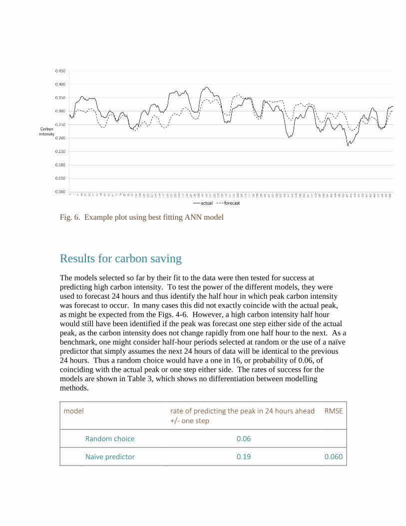
Fig. 6. Example plot using best fitting ANN model
Results for carbon saving
The models selected so far by their fit to the data were then tested for success at
predicting high carbon intensity. To test the power of the different models, they were
used to forecast 24 hours and thus identify the half hour in which peak carbon intensity
was forecast to occur. In many cases this did not exactly coincide with the actual peak,
as might be expected from the Figs. 4-6. However, a high carbon intensity half hour
would still have been identified if the peak was forecast one step either side of the actual
peak, as the carbon intensity does not change rapidly from one half hour to the next. As a
benchmark, one might consider half-hour periods selected at random or the use of a naïve
predictor that simply assumes the next 24 hours of data will be identical to the previous
24 hours. Thus a random choice would have a one in 16, or probability of 0.06, of
coinciding with the actual peak or one step either side. The rates of success for the
models are shown in Table 3, which shows no differentiation between modelling
methods.
model rate of predicting the peak in 24 hours ahead +/- one step
RMSE
Random choice 0.06
Naïve predictor 0.19 0.060

AR (400)(400)48 0.25 0.058
AR (200)(500)336 0.25 0.066
ANN 1-4, 48-52, 96-100, 336-340
0.25 0.056
Table 3. Rates of success in forecasting high carbon intensity
Finally, the success of these two models was assessed by calculating the carbon
saving achieved by DR determined by the model’s forecast of peak carbon intensity.
This was calculated as the average carbon intensity of the selected half hour periods over
the forecasting period. This can be compared with the average carbon intensity over the
same period, and the ratio expressed as an ‘improvement factor’. This period was of
different length for the different models because of the different quantity of initial values
each model needed. The results are shown in Table 4.
Best model
carbon intensity (kg/kWh) improvement factor period
average average saved
AR (400)(400)48 fig 4 0.298 0.358 1.20
AR
(200)(500)336 fig 5 0.303 0.349 1.15
ANN 1-4, 48-52, 96-100, 336-340
0.296 0.320 1.08
Table 4. Carbon saving results for selected models
Conclusion
The use of demand response is conventionally motivated by pricing signals whereby the
cost benefits of improved operation of the electricity grid are shared with consumers. In
this paper it has been shown that DR activity may be undertaken to reduce carbon
emissions directly. This use of DR may not provide the immediate commercial reward
but could be attractive to consumers valuing short-term impact on carbon emissions.

Many buildings use HVAC plant, which present useful loads for use in DR. It is to be
expected that switching plant off needs to be planned for and, therefore, advanced
warning of high carbon intensity would be useful. It has been shown that grid carbon
intensity exhibits a periodicity, and this can be exploited to develop forecast models. The
variation in carbon intensity can be forecast using linear autoregressive models or non-
linear ANN models. The models that best fit the time series are not necessarily best for
selecting when high carbon intensity is expected to occur. The modelling methods are
accessible to individual building operators as no exogenous data are used, but only data
in the public domain. Using the linear diurnally seasonal AR model to determine the
timing of DR can achieve an improvement in carbon emissions reduction of 20%. In
systems where the HVAC system load is displaced in time, the net reduction would also
depend on the carbon intensity at the new operating time. This is a tool for short-term
gain: increased use of DR and grid decarbonisation in the future should eventually
change the pattern of daily fluctuation and reduce the incidence of high carbon intensity.
Acknowledgments
Thanks are due to initial work undertaken by Selvaganapathy Swaminathan and Paul
Kamara while students at London South Bank University. This research received no
specific grant from any funding agency in the public, commercial, or not-for-profit
sectors.
References
1. C2ES. Outcomes of the UN Climate Change Conference in Paris. Arlington: Center
for Climate and Energy Solutions, 2015.
2. DECC. Memorandum to the Energy and Climate Change Committee: Post-legislative
Scrutiny of the Climate Change Act 2008 by the Secretary of State for the Department of
Energy and Climate. London: H.M.S.O, 2013.
3. Terry N. Energy and carbon emissions: the way we live today. UIT, 2011.
4. Bettle R, Pout CH and Hitchin ER. Interactions between electricity-saving measures
and carbon emissions from power generation in England and Wales. Energy Policy 2006;
34: 3434–3446. http://dx.doi.org/10.1016/j.enpol.2005.07.014
5. Hitchin R. A framework for building-related carbon coefficients and primary energy
factors for networked electricity supplies. Building Serv. Eng. Res. Technol. 2017;
http://dx.doi.org/10.1177/0143624417748507
6. Evans B and Sidat S. The use of temporal factors for improved CO2 emissions
accounting in buildings. Building Serv. Eng. Res. Technol. 2018; 39: 196-210
http://dx.doi.org/10.1177/0143624417753297

7. Harmsen R and Graus W. How much CO2 emissions do we reduce by saving
electricity? A focus on methods. Energy Policy 2013; 60: 803–812.
http://dx.doi.org/10.1016/j.enpol.2013.05.059
8. Hawkes AD. Long-run marginal CO2 emissions factors in national electricity systems.
Applied Energy 2014; 125: 197–205. http://dx.doi.org/10.1016/j.apenergy.2014.03.060
9. Graff Zivin JS, Kotchen MJ and Mansur ET. Spatial and temporal heterogeneity of
marginal emissions: Implications for electric cars and other electricity-shifting policies.
Journal of Economic Behavior & Organization 2014; 107: 248-268.
http://dx.doi.org/10.1016/j.jebo.2014.03.010
10. Voorspools KR and D’haeseleer WD. An evaluation method for calculating the
emission responsibility of specific electric applications. Energy Policy 2000; 28: 967-
980.
11. McCarthy R and Yang C. Determining marginal electricity for near-term plug-in and
fuel cell vehicle demands in California: Impacts on vehicle greenhouse gas emissions.
Journal of Power Sources 2010; 195: 2099–2109.
http://dx.doi.org/10.1016/j.jpowsour.2009.10.024
12. Hawkes AD. Long-run marginal CO2 emissions factors in national electricity
systems. Applied Energy 2014; 125: 197–205.
http://dx.doi.org/10.1016/j.apenergy.2014.03.060
13. Finenko A and Cheah L. Temporal CO2 emissions associated with electricity
generation: Case study of Singapore. Energy Policy 2016; 93: 70–79.
http://dx.doi.org/10.1016/j.enpol.2016.02.039
14. Hawkes AD. Estimating marginal CO2 emissions rates for national electricity
systems. Energy Policy 2010; 38: 5977–5987.
http://dx.doi.org/10.1016/j.enpol.2010.05.053
15. UKPN. Demand side response,
http://innovation.ukpowernetworks.co.uk/innovation/en/research-area/demand-side-
response/ (2016, accessed 27 July 2016).
16. Eissa MM. Demand side management program evaluation based on industrial and
commercial field data. Energy Policy 2011; 39: 5961–5969.
http://doi.org/10.1016/j.enpol.2011.06.057.
17. Ayón X, Gruber JK, Hayes BP, Usaola J and Prodanović M. An optimal day-ahead
load scheduling approach based on the flexibility of aggregate demands. Applied Energy
2017; 198 1–11. http://dx.doi.org/10.1016/j.apenergy.2017.04.038.
18. Motalleb M, Thornton M, Reihani E and Ghorbani R. A nascent market for
contingency reserve services using demand response. Applied Energy 2016; 179: 985–
995. http://dx.doi.org/10.1016/j.apenergy.2016.07.078.
19. Energy Networks Association. Smart Demand Response.
http://www.energynetworks.org/assets/files/news/publications/Smart_Demand_Response
_A_Discussion_Paper_July12.pdf (2012, accessed 4 May 2017).

20. Juneja S. Demand side response. London: OFGEM, 2010. Available from:
https://www.ofgem.gov.uk/ofgem-publications/57026/dsr-150710.pdf (accessed 22 July
2016).
21. Pedersen TH, Hedegaard RE and Petersen S. Space heating demand response
potential of retrofitted residential apartment blocks. Energy and Buildings 2017; 141:
158–166. http://dx.doi.org/10.1016/j.enbuild.2017.02.035
22. Ecotricity. Carbon content of UK Grid. https://www.ecotricity.co.uk/our-green-
energy/energy-independence/uk-grid-live (2017 accessed 25 May 2017).
23. GridCarbon, http://www.gridcarbon.uk [accessed 25.05.17].
24. UK Department for Business. Energy & Industrial Strategy. Greenhouse gas
reporting - Conversion factors 2016,
https://www.gov.uk/government/publications/greenhouse-gas-reporting-conversion-
factors-2016 (2016 accessed 25 May 2017).
25. Liu K, Subbarayan S, Shoults RR, Manry MT, Kwan C and Lewis, FI. Comparison of
very short-term load forecasting techniques. IEEE Transactions on Power Systems 1996;
11: 877–882. http://doi.org/10.1109/59.496169.
26. Hong WC. Electric load forecasting by support vector model. Applied Mathematical
Modelling 2009; 33: 2444–2454. http://doi.org/10.1016/j.apm.2008.07.010.
27. Almeshaiei E and Soltan H. A methodology for Electric Power Load Forecasting.
Alexandria Engineering Journal 2011; 50: 137–144.
http://dx.doi.org/10.1016/j.aej.2011.01.015.
28. Raza MQ and Khosravi A. A review on artificial intelligence based load demand
forecasting techniques for smart grid and buildings. Renewable and Sustainable Energy
Reviews 2015; 50: 1352–1372. http://doi.org/10.1016/j.rser.2015.04.065.
29. Deng J. Introduction to Grey System Theory. The Journal of Grey Systems 1989; 1:
1-24
30. Yao AWL, Chi SC and Chen JH. An improved Grey-based approach for electricity
demand forecasting. Electric Power Systems Research 2003; 67: 217-224.
https://doi.org/10.1016/S0378-7796(03)00112-3
31. Wang X, Qin H, Li Y, Tan Y and Cao Y. A Medium and Long-term Carbon Emission
Forecasting Method for Provincial Power Grid. 2014 International Conference on Power
System Technology (POWERCON 2014) Chengdu, 20-22 Oct. 2014.
32. Hsu C-C and Chen C-Y. Applications of improved grey prediction model for power
demand forecasting. Energy Conversion and Management 2003; 44: 2241–2249.
http://doi.org/10.1016/s0196-8904(02)00248-0.
33. Kayacan E, Ulutas B and Kaynak O. Grey system theory-based models in time series
prediction. Expert Systems with Applications 2010; 37: 1784-1789.
https://doi.org/10.1016/j.eswa.2009.07.064.

34. Pao, H-T, Fu, H-C and Tseng C-L. Forecasting of CO2 emissions, energy
consumption and economic growth in China using an improved grey model. Energy
2012; 40: 400–409. http://doi.org/10.1016/j.energy.2012.01.037.
35. Box GEP, Jenkins GM and Reinsel GC. Time series analysis: Forecasting and
control. 4th ed. United States: John Wiley & Sons, 2008.
36. Andalib A and Atry F. Multi-step ahead forecasts for electricity prices using NARX:
A new approach, a critical analysis of one-step ahead forecasts. Energy Conversion and
Management 2009; 50: 739–747 http://doi.org/10.1016/j.enconman.2008.09.040.
37. Beccali M, Cellura M, Lo Brano V and Marvuglia, A. Forecasting daily urban electric
load profiles using artificial neural networks. Energy Conversion and Management 2004;
45: 2879-2900. https://doi.org/10.1016/j.enconman.2004.01.006.
38. BuHamra S, Smaoui N and Gabr M. The Box-Jenkins analysis and neural networks:
prediction and time series modelling. Applied Mathematical Modelling 2003; 27: 805-
815. https://doi.org/10.1016/S0307-904X(03)00079-9.
39. Yalcinoz T and Eminoglu U. Short term and medium term power distribution load
forecasting by neural networks. Energy Conversion and Management 2005; 46: 1395-
1405. https://doi.org/10.1016/j.enconman.2004.07.005.
40. Kumar R, Aggarwal RK and Sharma JD. Energy analysis of a building using artificial
neural network: a review. Energy and Buildings 2013; 65: 352-358.
http://dx.doi.org/10.1016/j.enbuild.2013.06.007.
41. Li J, Shi J and Li J. Exploring Reduction Potential of Carbon Intensity Based on Back
Propagation Neural Network and Scenario Analysis: A Case of Beijing, China, Energies
2016; 9: 615. http://doi.org/10.3390/en9080615.
42. Short M, Crosbie T, Dawood M and Dawood N. Load forecasting and dispatch
optimisation for decentralised co-generation plant with dual energy storage. Applied
Energy 2017; 186: 304–320. http://dx.doi.org/10.1016/j.apenergy.2016.04.052.
43. Gridwatch. GB National Grid Status, http://www.gridwatch.templar.co.uk/ (2018
accessed 22 January 2018).
44. Gridwatch. UK Electricity National Grid CO2 Output per Production Type,
http://gridwatch.co.uk/co2-emissions (2017 accessed 25 May 2017).