technical report 16-04 - nagra · technical report 16-04 national cooperative for the disposal of...
TRANSCRIPT

TechnicalReport 16-04
National Cooperativefor the Disposal of Radioactive Waste
Hardstrasse 73CH-5430 Wettingen
SwitzerlandTel. +41 56 437 11 11
www.nagra.ch
December 2016
Modelling of Gas Generationin Deep Geological Repositories
after Closure
A. Poller, G. Mayer, M. Darcis & P. Smith


National Cooperativefor the Disposal of Radioactive Waste
Hardstrasse 73CH-5430 Wettingen
SwitzerlandTel. +41 56 437 11 11
www.nagra.ch
TechnicalReport 16-04
Modelling of Gas Generationin Deep Geological Repositories
after Closure
1 2 2 3A. Poller , G. Mayer , M. Darcis & P. Smith1) Nagra
2) AF-Consult Switzerland Ltd.3) SAM Switzerland Ltd.
December 2016

"Copyright © 2016 by Nagra, Wettingen (Switzerland) / All rights reserved.
All parts of this work are protected by copyright. Any utilisation outwith the remit of the
copyright law is unlawful and liable to prosecution. This applies in particular to translations,
storage and processing in electronic systems and programs, microfilms, reproductions, etc."
ISSN 1015-2636

I NAGRA NTB 16-04
Summary In deep geological repositories for radioactive waste, significant quantities of gases will be generated in the long term as a result of various processes, notably the anaerobic corrosion of metals and the degradation of organic materials. Therefore, the impact of gas production on post-closure safety of the repositories needs to be assessed as part of a safety case.
The present report provides a comprehensive description of the quantitative modelling of gas generation and associated water consumption during the post-closure phase of deep geological repositories in Opalinus Clay based on current scientific knowledge and on current preliminary repository designs. This includes a presentation of the modelling basis, namely the conceptual and mathematical models, the input data used, the computer tools developed, the relevant uncertainties and principal programme / design options, as well as the derivation, analysis and discussion of specific assessment cases.
The modelling is carried out separately for the two main sources of gas, which are the emplaced waste including the disposal containers; and the construction materials. The contribution of con-struction materials to gas generation rates in emplacement tunnels for spent fuel (SF) and vitrified high-level waste (HLW) is significant during several thousand years after closure. In the long term, however, the corrosion of the disposal canisters, which are in the reference case assumed to be fabricated of carbon steel, accounts for the vast majority of the total gas produced in these tunnels. The contribution of construction materials in emplacement caverns for long-lived intermediate-level waste (ILW) and low- and intermediate-level waste (L/ILW) to gas generation is generally small.
In ILW emplacement caverns, gas generation is generally dominated by hydrogen generation from the corrosion of cast iron Mosaik-II waste containers for PWR internals and from the corrosion of aluminium in operational waste from the surface facility of the HLW repository. In L/ILW emplacement caverns, gas production is also generally dominated by hydrogen genera-tion from the corrosion of carbon steel in decommissioning waste from the Beznau and Leibstadt reactors and from the PSI-West research facilities, although the contribution of the latter is apparently less pronounced according to recently updated inventory data. For both ILW and L/ILW, the degradation of organic materials does not significantly affect gas production.
The main factors of influence are found to be the amounts and geometric properties of carbon steel and aluminium, the associated corrosion mechanisms and corrosion rates, as well as the environmental conditions that prevail during the respective time periods for safety assessment. Some of these factors will be addressed with future research activities in order to further reduce the existing uncertainties. In addition, a number of programme and design options have the potential to markedly reduce gas generation if needed: the melting of metallic ILW and L/ILW, the use of alternative disposal canisters with substantially lower gas production for SF and HLW, the removal and / or replacement of ILW and L/ILW waste containers prior to disposal, as well as the use of non-rail-based technology for waste emplacement and backfilling in SF/HLW emplacement tunnels.

II NAGRA NTB 16-04
Zusammenfassung In geologischen Tiefenlagern für radioaktive Abfälle werden die anaerobe Korrosion von Metal-len und der Abbau von organischen Stoffen langfristig zur Bildung von signifikanten Gas-mengen führen. Die Auswirkungen der Gasbildung auf die Sicherheit der Tiefenlager nach deren Verschluss sind deshalb im Rahmen eines Sicherheitsnachweises vertieft zu untersuchen.
Der vorliegende Bericht beschreibt umfassend die quantitative Modellierung der Gasbildung und der zugehörigen Wasserzehrung während der Nachverschlussphase von geologischen Tie-fenlagern im Opalinuston basierend auf dem aktuellen wissenschaftlichen Kenntnisstand und auf gegenwärtigen vorläufigen Lagerauslegungen. Dies beinhaltet eine Darlegung der Model-lierungsgrundlagen, bestehend aus den konzeptionellen und mathematischen Modellen, den verwendeten Eingabedaten, den entwickelten Computerprogrammen und den relevanten Unge-wissheiten und Entsorgungs- bzw. Auslegungsvarianten, sowie auch die Herleitung, Analyse und Diskussion spezifischer Rechenfälle.
Die Modellierung erfolgt getrennt für die beiden Hauptgasquellen: Die einzulagernden Abfälle und deren Endlagerbehälter, sowie die Baumaterialen. Der Beitrag der Baumaterialien zu den Gasbildungsraten in Lagerstollen für abgebrannte Brennelemente (BE) und verglaste hochaktive Abfälle (HAA) ist während mehrerer tausend Jahre nach dem Verschluss sehr ausgeprägt. Längerfristig liefert jedoch die Korrosion der Endlagerbehälter, für welche im Referenzfall eine Herstellung aus Kohlenstoffstahl angenommen wird, den weitaus grössten Beitrag zu den gesamthaft gebildeten Gasmengen in diesen Lagerstollen. Der Beitrag der Baumaterialien zur Gasbildung in Lagerkammern für langlebige mittelaktive Abfälle (LMA) und für schwach- und mittelaktive Abfälle (SMA) ist generell gering.
In LMA-Lagerkammern wird die Gasbildung dominiert von der Wasserstoffbildung als Folge der Korrosion von gusseisernen Mosaik-II-Abfallbehältern für Reaktoreinbauten von Druck-wasserreaktoren, sowie der Korrosion von Aluminium in Betriebsabfällen der Oberflächen-anlage des HAA-Lagers. In SMA-Lagerkammern wird die Gasbildung dominiert von der Wasserstoffbildung durch die Korrosion von Stahl in Stilllegungsabfällen des KKB, des KKL und des PSI-West, wobei der Beitrag der PSI-West-Abfälle aufgrund kürzlich überarbeiteter Inventardaten offenbar deutlich geringer ist. Sowohl bei LMA, als auch bei SMA leistet der Abbau von organischen Stoffen keinen signifikanten Beitrag zur Gasproduktion.
Die wichtigsten Einflussgrössen sind die Mengen und geometrischen Eigenschaften von Stahl und Aluminium, die diesbezüglichen Korrosionsmechanismen und –raten, sowie die Umge-bungsbedingungen während der jeweiligen Betrachtungszeiträume. Für einige dieser Faktoren werden zukünftige Forschungsarbeiten zur Verringerung der bestehenden Ungewissheiten führen. Darüber hinaus haben zahlreiche Entsorgungs- und Auslegungsvarianten das Potenzial die Gasbildung bei Bedarf deutlich zu verringern: Das Einschmelzen von metallischen LMA und SMA, die Verwendung alternativer Behälter für BE und HAA mit deutlich verringerter Gasbildung, die Entfernung oder der Ersatz von Abfallbehältern unmittelbar vor der Einlage-rung, sowie der Einsatz von nicht-schienengebundener Technologie für die Einlagerung und die Verfüllung in BE/HAA-Lagerstollen.

III NAGRA NTB 16-04
Résumé Dans les dépôts pour déchets radioactifs aménagés en couches géologiques profondes, des quantités significatives de gaz seront générées au long terme, résultant de divers processus, en particulier de la corrosion anaérobie des métaux et de la dégradation des composés organiques. En conséquence, l'impact de la génération des gaz sur la sûreté des dépôts en phase post-fermeture doit être évalué dans le cadre d'une démonstration de sûreté.
Le présent rapport contient une description détaillée de la modélisation quantitative de la génération de gaz et de la consommation d'eau associée au cours de la phase post-fermeture des dépôts en couches géologiques profondes dans l'Argile à Opalinus, sur la base des connais-sances scientifiques actuelles et des conceptions de dépôts préliminaires existantes. Il présente la base de modélisation, c’est-à-dire les modèles conceptuels et mathématiques, les données d'entrée utilisées, les outils informatiques élaborés, les incertitudes pertinentes, les principales options stratégiques et conceptuelles, ainsi que la dérivation, l'analyse et la discussion de cas d'évaluation spécifiques.
La modélisation est réalisée séparément pour les deux sources de gaz principales, en l’occur-rence les déchets stockés (y compris les conteneurs de stockage) et les matériaux de construc-tion. La contribution des matériaux de construction au taux de génération de gaz dans les galeries de stockage pour assemblages combustibles usés (AC) et déchets de haute activité vitrifiés (DHA) est sensible sur plusieurs milliers d'années après la fermeture. Sur le long terme, toutefois, c’est la corrosion des conteneurs de stockage, fabriqués (selon le scénario de référence) en acier au carbone, qui est à l’origine de la majeure partie des gaz produits dans ces galeries. Les matériaux de construction présents dans les ouvrages souterrains pour déchets de moyenne activité à vie longue (DMA-VL) et de faible et moyenne activité (DFMA) ne contri-buent que pour une faible part à la génération de gaz.
Dans les ouvrages souterrains destinés au stockage des DMA-VL, la production de gaz est généralement due en majorité à la génération d'hydrogène issue de la corrosion des conteneurs de déchets radioactifs Mosaik-II en fonte utilisés pour les éléments internes des REP, ainsi que de la corrosion de l'aluminium dans les déchets d’exploitation provenant des installations de surface du dépôt pour DHA. Dans les ouvrages souterrains destinés au stockage des DFMA, la production de gaz est également due en majorité à la génération d'hydrogène issue de la corrosion de l'acier au carbone contenu dans les déchets de désaffectation provenant des réacteurs de Beznau et de Leibstadt, ainsi que du centre de recherche du PSI Ouest, bien que la contribution de ce dernier semble être moins prononcée si l’on considère les données d'inven-taire récemment mises à jour. Pour les DMA et DFMA, la dégradation des composés organiques n'affecte pas la production de gaz de manière significative.
La génération des gaz est principalement influencée par les quantités et les propriétés géomé-triques de l'acier au carbone et de l'aluminium, les mécanismes et taux de corrosion associés, ainsi que les conditions environnementales prédominantes au cours des périodes couvertes par les études de sûreté respectives. Certains de ces facteurs seront pris en compte lors d'activités de recherche ultérieures, afin de réduire les incertitudes existantes. En outre, on pourra avoir recours si nécessaire à certaines options stratégiques et conceptuelles qui permettront de réduire considérablement la génération de gaz: la fusion des DMA et DFMA métalliques, l'utilisation, pour les AC et DHA, de conteneurs de stockage dont les matériaux génèrent des quantités de gaz bien inférieures, le retrait et/ou le remplacement de conteneurs de DFMA et DMA avant stockage, ainsi que le choix de technologies fonctionnant sans rails pour la mise en place des colis et le remblayage des ouvrages souterrains destinés aux AC/DHA.


V NAGRA NTB 16-04
Table of Contents
Summary ................................................................................................................................... I
Zusammenfassung ......................................................................................................................... II
Résumé ................................................................................................................................ III
Table of Contents .......................................................................................................................... V
List of Tables .............................................................................................................................. VII
List of Figures ............................................................................................................................. IX
1 Introduction ............................................................................................................ 1 1.1 Background and aims ............................................................................................... 1 1.2 Regulatory requirements ........................................................................................... 2 1.3 Overview of earlier studies and recent international activities ................................. 3 1.4 Organisation of the report ......................................................................................... 4
2 Model Description ................................................................................................... 5 2.1 Conceptual model ..................................................................................................... 5 2.1.1 General ...................................................................................................................... 5 2.1.2 Degradation of organic materials .............................................................................. 8 2.1.3 Corrosion of metals .................................................................................................. 9 2.2 Mathematical model ............................................................................................... 10 2.2.1 Gas production and water consumption ................................................................. 10 2.2.2 Degradation of organic materials ............................................................................ 12 2.2.3 Corrosion of metals ................................................................................................ 12 2.3 Input data ................................................................................................................ 15 2.3.1 Waste and disposal containers ................................................................................ 15 2.3.2 Construction materials ............................................................................................ 17 2.4 Computer tools ....................................................................................................... 19 2.4.1 User interface .......................................................................................................... 20 2.4.2 Workflow and internal structure ............................................................................. 23 2.4.3 Verification ............................................................................................................. 23 2.5 Assessment cases .................................................................................................... 25 2.5.1 Summary of uncertainties and options.................................................................... 25 2.5.2 Waste and disposal containers ................................................................................ 26 2.5.3 Construction materials ............................................................................................ 33
3 Results and Discussion ......................................................................................... 35 3.1 Waste and disposal containers ................................................................................ 35 3.1.1 Base case ................................................................................................................. 35 3.1.2 Uncertainties ........................................................................................................... 59

NAGRA NTB 16-04 VI
3.1.3 Options.................................................................................................................... 74 3.1.4 Bounding cases ....................................................................................................... 87 3.2 Construction materials ............................................................................................ 95 3.2.1 Base case ................................................................................................................. 95 3.2.2 Uncertainties ......................................................................................................... 103 3.2.3 Options.................................................................................................................. 106 3.2.4 Bounding cases ..................................................................................................... 109 3.3 Comparison for emplacement rooms .................................................................... 111
4 Conclusions .......................................................................................................... 121
References .............................................................................................................................. 125
A Model Reactions and Parameter Values ........................................................... A-1
B Amounts and Properties of Gas-generating Materials .................................... B-1 B.1 Waste and disposal containers .............................................................................. B-1 B.1.1 Base scenario ........................................................................................................ B-3 B.1.2 Alternative waste scenarios .................................................................................. B-8 B.2 Construction materials ........................................................................................ B-15
C Glossary ............................................................................................................... C-1

VII NAGRA NTB 16-04
List of Tables
Tab. 2-1: Profiles and corresponding locations in the HLW repository and the L/ILW repository. ............................................................................................................... 18
Tab. 2-2: Summary of key uncertainties and principal programme and design options. ....... 26
Tab. 2-3: Assessment cases for waste and disposal containers. ............................................. 31
Tab. 2-4: Assessment cases for construction materials. ......................................................... 33
Tab. 3-1: Total amounts of gas produced and water consumed by the end of the respective time frames for safety assessment in the base case. .............................. 49
Tab. 3-2: Intensely gas-producing ILW sorts and predominant waste sorts (bold) along with the most relevant waste object within each waste sort in the base case. ........ 56
Tab. 3-3: Intensely gas-producing L/ILW sorts and predominant waste sorts (bold) along with the most relevant waste object in each waste sort in the base case. ...... 57
Tab. 3-4: Waste sorts in the ILW and L/ILW repository that are subject to waste treatment options and waste volumes involved for different alternative waste scenarios. ...................................................................................................... 80
Tab. 3-5: Waste in the L/ILW repository resulting from waste treatment options and waste volumes for different alternative waste scenarios. ....................................... 82
Tab. 3-6: Total amounts of gas produced and water consumed from L/ILW by the end of the time frame for safety assessment for different alternative waste scenarios. ................................................................................................................ 83
Tab. 3-7: Total amounts of gas produced [m3 SATP] and water consumed [kg] by the end of the respective time frames for safety assessment in the base case(s) and in the bounding cases. ...................................................................................... 92
Tab. 3-8: Total amounts of gas produced and water consumed [mol] by the end of the respective time frames for safety assessment in the base case(s) and in the bounding cases. ....................................................................................................... 94
Tab. 3-9: Comparison of total amounts of gas produced [m3 SATP] and water consumed [kg] from waste and disposal containers vs. construction materials by the end of the respective time frames for safety assessment in the base case. ...................................................................................................................... 112
Tab. A-1: Model reactions. ................................................................................................... A-1
Tab. A-2: Parameter values for model reactions. .................................................................. A-4
Tab. B-1: Gas-generating MIRAM 14 standard materials and corresponding model precursor substances (both in German). ............................................................... B-1
Tab. B-2: Profiles of the HLW repository and the L/ILW repository with corresponding construction materials, material masses, corrosion models and corrosion classes. ................................................................................................ B-15
Tab. C-1: Glossary of terms, abbreviations and acronyms. .................................................. C-1


IX NAGRA NTB 16-04
List of Figures
Fig. 2-1: Screenshot showing the graphical user interface (GUI) in the sheet "Ergebnisse" of the gas generation tool for emplaced waste, including disposal containers. ................................................................................................. 21
Fig. 2-2: Screenshot showing some of the filter options in the sheet "Inventare" of the gas generation tool for emplaced waste, including disposal containers. ................ 22
Fig. 2-3: Simplified sketch of the general workflow in the gas generation tools. ................. 23
Fig. 2-4: List of the individual sheets in the gas generation tools. ........................................ 24
Fig. 3-1: Gross production of different gas species from SF in the base case. ...................... 38
Fig. 3-2: Gross production of different gas species from HLW in the base case. ................. 39
Fig. 3-3: Gross production of different gas species from ILW-AG1 in the base case........... 40
Fig. 3-4: Gross production of different gas species from ILW-AG2 in the base case........... 41
Fig. 3-5: Gross production of different gas species from L/ILW-AG1 in the base case. ...... 42
Fig. 3-6: Gross production of different gas species from L/ILW-AG2 in the base case. ...... 43
Fig. 3-7: Net gas production for the different waste categories in the base case. ................. 45
Fig. 3-8: Water consumption for the different waste categories in the base case. ................ 47
Fig. 3-9: Evolution of the average water consumption factor for metals and organic materials for the different waste categories in the base case. ................................. 48
Fig. 3-10: Gas production from ILW-AG1 in the base case with details on the contribution of different metals and of the ensemble of organic materials. ........... 50
Fig. 3-11: Gas production from ILW-AG2 in the base case with details on the contribution of different metals and of the ensemble of organic materials. ........... 51
Fig. 3-12: Gas production from L/ILW-AG1 in the base case with details on the contribution of different metals and of the ensemble of organic materials. ........... 52
Fig. 3-13: Gas production from L/ILW-AG2 in the base case with details on the contribution of different metals and of the ensemble of organic materials. ........... 53
Fig. 3-14: Gas production from SF and HLW for the base cases and for alternative cases with upper and lower bound corrosion rates. ................................................ 61
Fig. 3-15: Gas production from ILW-AG1 and ILW-AG2 for the base cases and for alternative cases with upper and lower bound corrosion rates. .............................. 62
Fig. 3-16: Gas production from L/ILW-AG1 and L/ILW-AG2 for the base cases and for alternative cases with upper and lower bound corrosion rates. ......................... 63
Fig. 3-17: Gas production from ILW-AG1 and ILW-AG2 for the base cases and for alternative cases with upper and lower bound degradation rates. ........................... 65
Fig. 3-18: Gas production from L/ILW-AG1 and L/ILW-AG2 for the base cases and for alternative cases with upper and lower bound degradation rates. ..................... 66
Fig. 3-19: Gas production from ILW-AG1 and ILW-AG2 for the base cases and for alternative cases with no pH change due to the degradation of organic materials. ................................................................................................................. 68

NAGRA NTB 16-04 X
Fig. 3-20: Gas production from L/ILW-AG1 and L/ILW-AG2 for the base cases and for alternative cases with no pH change due to the degradation of organic materials. ................................................................................................................. 69
Fig. 3-21: Gas production from ILW for the base cases and for alternative cases with waste allocations to a single emplacement room with high and low gas production. .............................................................................................................. 71
Fig. 3-22: Gas production from L/ILW for the base cases and for alternative cases with waste allocations to a single emplacement room with high and low gas production. .............................................................................................................. 72
Fig. 3-23: Gas production from ILW-AG1 for the base case and for alternative cases in which all drums are removed and/or Mosaik-II waste containers are replaced. .................................................................................................................. 75
Fig. 3-24: Gas production from ILW-AG2 for the base case and for alternative cases in which all drums are removed and/or Mosaik-II waste containers are replaced. .................................................................................................................. 76
Fig. 3-25: Gas production from L/ILW-AG1 for the base case and for alternative cases in which all drums are removed and/or Mosaik-II waste containers are replaced. .................................................................................................................. 77
Fig. 3-26: Gas production from L/ILW-AG2 for the base case and for alternative cases in which all drums are removed and Mosaik-II waste containers are replaced. ..... 78
Fig. 3-27: Gas production from L/ILW for the base case assuming different waste scenarios. ................................................................................................................ 84
Fig. 3-28: Gas production from SF and HLW for the base cases and for the cases assuming an alternative disposal canister. .............................................................. 86
Fig. 3-29: Gas production from SF and HLW for the base cases and the upper and lower bounding cases. ............................................................................................. 88
Fig. 3-30: Gas production from ILW for the base cases and for the upper and lower bounding cases. ....................................................................................................... 90
Fig. 3-31: Gas production from L/ILW for the base cases and for the upper and lower bounding cases. ....................................................................................................... 91
Fig. 3-32: Gas production for different profiles in the base case. ........................................... 96
Fig. 3-33: Water consumption for different profiles in the base case. .................................... 98
Fig. 3-34: Gas production in SF / HLW emplacement tunnels (profiles F / ZS) in the base case with details on individual construction components. ............................ 100
Fig. 3-35: Gas production in ILW emplacement caverns (profile K04) in the base case with details on individual construction components. ............................................ 101
Fig. 3-36: Gas production in L/ILW emplacement caverns (profile K09) in the base case with details on individual construction components. .................................... 102
Fig. 3-37: Gas production in individual emplacement room profiles for the base cases and for alternative cases with upper bound and lower bound corrosion rates. ..... 104
Fig. 3-38: Gas production in individual emplacement room profiles for the base cases and for alternative cases with upper bound and lower bound values for the amounts of construction materials. ....................................................................... 105

XI NAGRA NTB 16-04
Fig. 3-39: Gas production in profile ZS (interjacent sealing section) for the base case and for an alternative case with tunnel support provided by liner. ....................... 107
Fig. 3-40: Gas production in profiles F (emplacement section) and ZS (interjacent sealing section) for the base cases and for alternative cases with rail-based emplacement and backfilling technology. ............................................................ 108
Fig. 3-41: Gas production in individual emplacement room profiles for the base cases and for the upper and lower bounding cases. ........................................................ 110
Fig. 3-42: Comparison of gas production from waste and disposal containers vs. construction materials in an SF emplacement tunnel. .......................................... 114
Fig. 3-43: Comparison of gas production from waste and disposal containers vs. construction materials in an HLW emplacement tunnel. ...................................... 115
Fig. 3-44: Comparison of gas production from waste and disposal containers vs. construction materials in an ILW emplacement room. ......................................... 117
Fig. 3-45: Comparison of gas production from waste and disposal containers vs. construction materials in an L/ILW emplacement room. ..................................... 119
Fig. B-1: Total mass, volume-specific mass and mass contributions of model precursor substances for SF (upper figures) and HLW (lower figures) in the base scenario. ................................................................................................................ B-3
Fig. B-2: Total mass, volume-specific mass and mass composition of model precursor substances for ILW-AG1 in the base scenario. ..................................................... B-4
Fig. B-3: Total mass, volume-specific mass and mass composition of model precursor substances for ILW-AG2 in the base scenario. ..................................................... B-5
Fig. B-4: Total mass, volume-specific mass and mass composition of model precursor substances for L/ILW-AG1 in the base scenario. ................................................. B-6
Fig. B-5: Total mass, volume-specific mass and mass composition of model precursor substances for L/ILW-AG2 in the base scenario. ................................................. B-7
Fig. B-6: Total mass, volume-specific mass and mass composition of model precursor substances for L/ILW in the base scenario. .......................................................... B-8
Fig. B-7: Total mass, volume-specific mass and mass composition of model precursor substances for L/ILW in the alternative waste scenario with pyrolysis (M14AP). .............................................................................................................. B-9
Fig. B-8: Total mass, volume-specific mass and mass composition of model precursor substances for L/ILW in the hypothetical alternative waste scenario with total pyrolysis (M14APA). ................................................................................. B-10
Fig. B-9: Total mass, volume-specific mass and mass composition of model precursor substances for L/ILW in the alternative waste scenario with melting (M14AS). ............................................................................................................ B-11
Fig. B-10: Total mass, volume-specific mass and mass composition of model precursor substances for L/ILW in the alternative waste scenario with pyrolysis and melting (combination of M14AP and M14AS). ................................................. B-12
Fig. B-11: Total mass, volume-specific mass and mass composition of model precursor substances for L/ILW in the alternative waste scenario with the updated inventory of decommissioning waste from the PSI-West research facility (M14A U PSIW). ................................................................................................ B-13

NAGRA NTB 16-04 XII
Fig. B-12: Total mass, volume-specific mass and mass composition of model precursor substances for L/ILW in the alternative waste scenario with the updated inventory of decommissioning waste from the PSI-West research facility and melting (M14AS U PSIW). ................................................................................ B-14

1 NAGRA NTB 16-04
1 Introduction
1.1 Background and aims
In Switzerland, the Nuclear Energy Act requires the disposal of all types of radioactive waste in deep geological repositories (NEA 2003). A deep geological repository is described as an installation located deep underground, which may be closed once the permanent protection of humans and the environment is ensured through a system of passive safety barriers. It comprises a main facility for the emplacement of the radioactive waste, a pilot facility and test areas, along with the underground access structures to these facilities.
The overall approach to implementing deep geological disposal in Switzerland is set out in the Waste Management Programme (Nagra 2016a). This programme foresees two types of deep geological repository: a high-level waste repository (HLW repository) for spent fuel (SF), vitrified high-level waste (HLW) and long-lived intermediate-level waste (ILW)1; and a repository for low- and intermediate-level waste (L/ILW repository).2
The procedure and the criteria for the selection of sites for the deep geological repositories are specified in the conceptual part of the "Sectoral Plan for Deep Geological Repositories" (SFOE 2008). The procedure consists of three stages and will ultimately lead to the identification of the sites for repository implementation, the definition of the main features of the repositories and the granting of the general licences. In Stage 1 of the Sectoral Plan, potential host rocks and associated geological siting regions were identified and entered into the Sectoral Plan with a decision by the Federal Council (SFOE 2011). In the course of Stage 2, Nagra proposed the two geological siting regions Jura Ost and Zürich Nordost for both repository types for further investigation in Stage 3 (Nagra 2014a).
After closure of a deep geological repository, significant quantities of gases will be generated in the long term as a result of various processes, most notably the anaerobic corrosion of metals and the degradation of organic materials. In order to make the case for the safety of the repository after closure, the potential impact of gas production on post-closure safety needs to be assessed.
The main objective of the present report is to provide quantitative estimates of gas generation rates and associated water consumption rates for the post-closure phase of deep geological repositories in Opalinus Clay based on current scientific knowledge and current preliminary repository designs.3 The modelling of gas generation and water consumption does not explicitly consider the coupling with other related processes, namely the transport of gas and water as well as the possible consumption of gas, for which the present results are used as source terms. The scope of the present report is thus limited to the modelling of gas production and water consumption. The related modelling of gas / water transport is documented in Papafotiou & Senger (2016a/b). A comprehensive treatment of possible gas consumption processes in the L/ILW repository is documented in Leupin et al. (2016c). The overall assessment of the impact of gas pressure build-up on post-closure safety is documented in a gas synthesis report (Diomidis et al. 2016). 1 There is also the possibility to dispose of ILW in the L/ILW repository. 2 There is also the possibility to construct the HLW repository and the L/ILW repository at the same site, i.e. a so-
called combined repository. Gas generation in such a combined repository is not dealt with explicitly in the present report, although it can in principle be inferred from the results that are documented herein.
3 This report does not address the generation of radioactive gases, since these are insignificant in terms of gas volume produced and the resulting gas pressure build-up.
NAGRA NTB 16-04 2
The scientific basis that underpins the gas generation and water consumption model is also not documented in the present report. A synopsis is given in the gas synthesis report (Diomidis et al. 2016) and more details can be found in Diomidis (2014), Cloet et al. (2014), Warthmann et al. (2013a), Warthmann et al. (2013b) and Newman et al. (2015).
Further objectives of this report are:
to document the gas generation and water consumption models in a clear and traceable manner;
to identify the materials and waste types that dominate gas generation and water consumption;
to show the impact of various model and parameter uncertainties;
to show the impact of design options, specifically those available
for the SF/HLW disposal canister material,
for tunnel support at the location of seals, and
for the emplacement of SF and HLW;
to show the impact of programme options regarding currently available processes that are capable of reducing and / or avoiding organic and metallic materials in ILW and L/ILW.
1.2 Regulatory requirements
On the subject of post-closure gas generation, the regulatory guideline on design principles for deep geological repositories and on requirements for the safety case (ENSI 2009a) contains the following statement:
Safety assessment as part of a safety case needs to include: Description of the expected evolution of the materials in the repository, including the radioactive waste and the engineered and natural barriers. The description has to take into account possible mutual influences of the different materials.
The explanatory report on ENSI (2009a) requires further that the generation of gases be monitored in the pilot repository and that safety analyses include the description of the evolution of the technical barriers, e.g. the corrosion behaviour of disposal canisters (ENSI 2009b).
More generally, the need to assess the consequences of gas generation on post-closure safety also arises from the regulatory principle of optimisation in ENSI (2009a), which is understood as a continuous process in which various relevant alternatives and their significance for operational and post-closure safety are considered for every safety-relevant aspect, thus leading to a decision that is favourable overall for safety and reasonable from the perspective of the state-of-the-art in science and technology.
ENSI (2015) contains additional recommendations, stipulating an in-depth analysis and safety-related evaluation of
currently available processes capable of reducing and / or avoiding organic and metallic materials in ILW and L/ILW; and
alternative materials for the fabrication of SF/HLW disposal canisters.

3 NAGRA NTB 16-04
These efforts are documented in the framework of the Waste Management Programme 2016 (Nagra 2016a) and the associated Research, Development and Demonstration (RD&D) Plan 2016 (Nagra 2016b).
1.3 Overview of earlier studies and recent international activities
The modelling of gas generation has been part of several Nagra studies that have investigated the potential impact of gas production on the post-closure safety of a deep geological repository. The most recent and most comprehensive investigation for the HLW repository is documented in Nagra (2004); a similar assessment for the L/ILW repository is reported in Nagra (2008). Both documents focus on gas generation from the emplaced waste, including the disposal containers. The most recent estimates of gas production rates from construction materials and other materials that remain in the emplacement rooms are given in Nagra (2011).
Gas generation has also been modelled within the framework of several foreign radioactive waste management programmes. The following gives a brief overview of recent activities in other programmes, with the focus on the tools used and the main processes implemented in the respective tools:
Project SAFE (Safety Assessment of Final Repository for Radioactive Operational Waste) was undertaken by SKB in the period up to 2001 to meet the licensing requirement that a revised safety assessment for the SFR 1 repository for L/ILW at Forsmark, Sweden, has to be carried out every 10 years during the continued operation of the facility. As part of SAFE, radionuclide release from the repository caused by gas generation was analysed, as reported in Moreno et al. (2001). Gas generation modelling considered the hydrogen produced by corrosion of metals, by microbial degradation of organic materials and by radiolytic decomposition of water.
A modelling tool for assessing gas generation during the transport, underground disposal and repository post-closure phases for ILW and certain types of LLW was developed in the UK on behalf of United Kingdom Nirex Limited. The modelling tool has since been continuously updated and the latest version is reported in Swift (2016a/b). The main gas-generating processes represented by the tool, SMOGG, are corrosion of metals, radiolysis, microbial degradation of organic molecules and radioactive decay. The main output of the tool is the production rate of bulk gases (hydrogen, carbon dioxide and methane) and the release of radioactive gases (gaseous species containing H-3 and C-14 and Rn-222, Kr-81, Kr-85, Ar-39 and Ar-42).
Canada's NWMO developed a modelling tool that can be used to analyse both the generation and transport of gases in a deep geological repository for L/ILW (NWMO 2011). The tool, T2GGM, is comprised of two coupled models: a Gas Generation Model (GGM) and a TOUGH2 model for gas/water transport within the repository system. The main processes represented by the GGM are corrosion product and hydrogen gas generation from the corrosion of steels and other alloys, as well as CO2 and CH4 gas generation from the degradation of organic materials, all under either aerobic or anaerobic conditions.
Belgium's ONDRAF/NIRAS has presented a modelling study of gas production from SF, HLW, compacted waste (hulls, end-pieces, etc.) and waste in Mosaik containers from the dismantling of lower core internals of Belgian PWRs (Yu & Weetjens 2012). The main source of gas in each case is the corrosion of metals. For example, in the case of SF, gas production comes mainly from the anaerobic corrosion of the carbon steel overpack, the cast iron supporting frame, the stainless steel assembly boxes and the various metals contained in the fuel assembly. In the case of HLW, the main source of gas is the anaerobic corrosion of the overpack and the waste canisters.

NAGRA NTB 16-04 4
In France, ANDRA has presented a study dealing with gas generation and gas transport in the context of the project Dossier 2005 (Talandier 2005). The gas generation model used incorporates the anaerobic corrosion of metals, the radiolysis of organic materials, the microbial degradation of organic materials, the radiolysis of water and radioactive decay. Gas generation rates are calculated for a number of different high-level waste categories (Déchets C) and intermediate-level waste categories (Déchets B). The gas sources addressed are the waste, any additional containment and the underground construction materials.
In addition, gas generation has been addressed in the pan-European FORGE (Fate Of Repository GasEs) project that ran from 2009 to 2013. The project, with partners from 24 organisations in 12 European countries, had links to international radioactive waste management organisations, regulators and academia. It was specifically designed to tackle the key research issues associated with the generation and movement of repository gases. Key findings are presented in a synthesis report (Norris et al. 2013). Work Package 2 of FORGE dealt with gas generation, especially due to the corrosion of metals. Specific issues addressed included the effects of redox conditions, temperature and the presence of bentonite on gas generation, as well as the effects of gamma radiation on the corrosion of steel in clay porewater. Microbial corrosion was not studied in FORGE, but it was noted that further in-situ studies may be warranted.
1.4 Organisation of the report
The model used to calculate gas generation and water consumption in deep geological repositories is presented in Chapter 2. This includes a detailed description of the conceptual and mathematical model, the input data used and an overview of the computer tools used to calculate gas generation and water consumption. It also includes a summary of relevant uncertainties, which lays the foundation for the definition of assessment cases.
Chapter 3 presents the model results separately for the two main sources of gas in a deep geological repository: the emplaced waste, including the disposal containers, and the con-struction materials (including other materials that remain underground after repository closure). In addition to the results for the respective base cases, the influence of model and parameter uncertainties, as well as the impact of selected design and programme options on gas generation, is investigated for the two main sources of gas in a systematic and deterministic manner. Thereafter, bounding cases for use in related studies on gas / water transport and gas consumption are constructed based on the findings of the preceding uncertainty analyses. Finally, gas production from the waste and the construction materials in the different types of emplacement room is compared, including the uncertainties as expressed through the respective bounding cases.
The conclusions of the present modelling study are presented in Chapter 4. Appendix A lists the model reactions and parameter values used in the gas generation model. Appendix B contains quantitative information on amounts and properties of those materials in the repositories that are potentially involved in gas generation reactions. Appendix C provides a glossary of terms, abbreviations and acronyms.

5 NAGRA NTB 16-04
2 Model Description
2.1 Conceptual model
The conceptual model draws upon the current state of scientific knowledge of metal corrosion and degradation of organic materials under repository conditions. It is described in detail in Diomidis (2014), Cloet et al. (2014), Warthmann et al. (2013a), Warthmann et al. (2013b) and Newman et al. (2015). The repository conditions and their expected evolution are discussed in a more general context in Kosakowski et al. (2014) and in Bradbury et al. (2014). An overview of the scientific basis of gas generation is given in the gas synthesis report (Diomidis et al. 2016).
2.1.1 General
The start time of the model is taken to coincide with the end of the operational phase of a deep geological repository, i.e. with the beginning of the post-closure phase. It is assumed that waste emplacement and closure of the repository occur simultaneously and instantaneously at this start time. It is further assumed that the gas-generating materials are not altered prior to this start time (e.g. by aerobic corrosion during interim storage).4
For illustrative purposes, the modelling period extends to 107 years after closure, although a number of assumptions may not be strictly valid beyond the respective time frames for safety assessment, which are 105 years for the L/ILW repository and 106 years for the HLW repository.5
Any substance or material in the repository that potentially contributes to gas generation during the post-closure phase is considered as a component of the gas generation model. There are two main sources of gas in a deep geological repository: the emplaced waste, including the disposal containers, and the construction materials needed to support the underground structures, along with other gas-producing materials that will remain in the repository. Gas generation is calculated separately for these two sources (cf. below).
In order to reduce the number of components to be treated explicitly in the model, each substance / material is, in the first instance, assigned to a model precursor substance A, which may be either a corroding metal M or a degradable organic substance O. The different model precursor substances taken into account are listed in Appendix A. Information on total and volume-specific amounts of model precursor substances in the different repositories and on relevant material properties are provided in Appendix B.
Every model precursor substance A is assumed to react independently6 and irreversibly according to the following generic gas generation reaction:
A H2O Eadditionalreactants
env.conditions,catalysts
G gaseousproducts
Padditionalproducts
4 Simplified calculations have shown that the expected effect is too small to require explicit consideration. 5 In the presentation of the results in Chapter 3, the times beyond the respective time frame for safety assessment
are indicated with a shaded region. 6 This assumption states that the individual model precursor substances do not react with each other, which
maximises gas production. The opposite case is bounded by the lower bound degradation rates, which are set to zero. Note that indirect couplings such as locally enhanced corrosion due to degradation of organic material are taken into account.

NAGRA NTB 16-04 6
A specific model reaction is defined for each model precursor substance A (see Appendix A). For instance, the model precursor substance Na-polystyrene-sulphonate is assumed to be degraded by microbes under reducing conditions according to
C8H7SO3Na 5H2O aq H → 4CO2 4CH H S Na .
The model reactions are generally representative of the sum of several partial reactions and it is assumed that the turnover of the model precursor substances goes to completion, which maximises gas production. Furthermore, water is produced in some reactions, which is accounted for by using a negative value for .
The formulation of the model reactions is such that the maximum amount of gas is produced. For instance, Fe may be transformed into Fe3O4 or Fe(OH)2, depending on the environmental conditions (Diomidis 2014). Since the formation of Fe3O4 yields more hydrogen per mole of Fe, this type of reaction is taken as the representative model reaction.
The environmental conditions that control the reactions (e.g. temperature, concentration / partial pressure of reactants and products, availability of catalysts, salinity, pH, redox potential) are reflected in the corrosion and degradation rates given for the individual model reactions (see Appendix A). It is further assumed that corrosion and degradation rates are constant throughout the modelling period. Any uncertainties with respect to the environmental conditions (including their evolution and spatial variability) are included in the uncertainties given for the constant corrosion and degradation rates.
Generally, production, transport and consumption of gas and water in a closed deep geological repository are coupled processes. On the one hand, gas and water transport affect the produc-tion / consumption of water and gas, e.g. by controlling the gas pressure and the availability of water for corrosion and degradation reactions. On the other hand, water and gas produc-tion / consumption will influence the movement of water and gas.7 Overall, a modelling approach is adopted that does not explicitly consider the coupling between gas production / water consumption and the other processes mentioned. As a consequence, the full range of possible outcomes of gas generation and water consumption needs to feed into the modelling of the related processes. Likewise, the full range of possible outcomes of these related processes needs to be considered for modelling gas generation and water consumption. Bounding assump-tions are therefore incorporated into the uncertainties given for the constant corrosion and degradation rates. For instance, the lower bound degradation rates reflect the possibility that water saturation is so low that degradation of organic materials due to microbial activity cannot occur. Thus, the results presented in this report will fall below or exceed the outcomes to be realistically expected to some extent, which needs to be recognised in related modelling and assessment activities.
In a deep geological repository according to Nagra's reference disposal concept, two principal types of chemical environment can be distinguished: (i) a cementitious environment with relatively high pH values in ILW and L/ILW emplacement rooms (or caverns) and in all concrete structures throughout the repository system, and (ii) a so-called "clay environment" with near-neutral pH values at all other locations. Recent experimental evidence suggests that any oxygen trapped in the repository upon closure may be consumed rather rapidly (Mueller et al. 2017). The model therefore assumes reducing conditions for both types of chemical environment throughout the modelling period. 7 The effect of water consumption may however be small, provided the hydraulic conductivity of the host rock
exceeds a threshold value of about 10-14 m/s (Senger et al. 2008), which is the case for Opalinus Clay in the proposed geological siting regions.

7 NAGRA NTB 16-04
For the model precursor substances "Iron, Carbon steel: anaerobic corrosion" and "Stainless steel, Ni-alloys: anaerobic corrosion", which are by far the dominant materials in terms of total mass (see Appendix B), different corrosion rates are provided for the clay environment (pH < 10.5) and for the cementitious environment (pH ≥ 10.5) in Diomidis (2014). In the case of potentially degraded cement, corrosion rates representative of the clay environment are applied, which tends to maximise gas production rates. For the remaining model corrosion reactions, the same corrosion rates are applied in the two environments and the corresponding bounding values cover both environments. The degradation rates of organic materials are valid for the cementitious environment; only small amounts of organic materials are present in the clay environment and are thus not represented in the model.
Since the gas generation model does not account for transport and accumulation processes, no spatial model domain is defined. However, different waste categories will be emplaced at separate locations in the repositories; hence there is at least an implicit spatial reference through the individual waste categories. The different waste categories distinguished are spent fuel (SF), vitrified high-level waste (HLW), long-lived intermediate-level waste (ILW) and low-/intermediate-level waste (L/ILW) (see Section 2.3.1).
ILW and L/ILW are each further subdivided into two different waste groups based on criteria related to radionuclide mobility in order to optimise overall radionuclide retention in the near-field (cf. Cloet et al. 2014). The resulting waste categories ILW-AG1 and ILW-AG2, as well as L/ILW-AG1 and L/ILW-AG2, will be emplaced in separate emplacement caverns. Accordingly, gas production is calculated separately for the different waste groups of ILW and L/ILW. Gas generation from construction materials is calculated per unit length for different types of emplacement room (hereafter called room profiles or simply profiles), which also provides for an implicit spatial reference.
Only the corrosion of metals and the degradation of organic materials are considered in the present model. The contribution of gas produced from radiolysis of water or from radiolysis of organic materials is ignored. These simplifications are backed up by the results of earlier Nagra studies (cf. Nagra 2004) and international consensus (e.g. FORGE synthesis report; Norris et al. 2013).8
It is generally assumed that gas production from the waste itself is not delayed by the waste containers.9 The exception to this rule concerns the breaching of the SF/HLW disposal canisters, which causes a sudden rise in the canister surface area available for corrosion and a sudden start of gas production from other materials originally contained within the canister. The reference assumption is that breaching of all SF/HLW disposal canisters occurs at 10,000 years.10
For the sake of consistency with earlier assessments, the calculated gas generation rates and the cumulative amounts of produced gas are presented primarily in volumetric quantities, notwithstanding the fact that part or all of the produced gas may react or dissolve at its point of origin and thus does not contribute to the formation of a gas phase. The volumetric quantities 8 The contribution of radiolysis will be reviewed in preparation for the upcoming general licence applications. 9 This assumption results from a detailed analysis of the different ILW and L/ILW waste types, which revealed that
only small cylinders and Mosaik-II waste containers may be capable of providing substantial containment. However, the relative amount of gas that is potentially produced from waste inside these types of containers is generally small (< 5 vol.-%) for all ILW and L/ILW waste categories and for different sub-periods of the respective time frames for safety assessment.
10 In reality, the individual SF/HLW disposal canisters will breach at different times, with 10,000 years being the lower limit of this distribution in time. Overall, the adopted approach tends to overestimate gas production at 10,000 years.

NAGRA NTB 16-04 8
are given for standard ambient temperature and pressure conditions (SATP), which assume a gas pressure of 105 Pa and a temperature of 25 °C. The contributions of the different model precursor substances are summed for each waste category. This implies that the resulting gas mixture can be described by the ideal gas law.
Gas generation rates are calculated both in total amounts for each waste category and per unit volume of packaged waste for each waste category, since the latter parameter is the key quantity for gas pressure build-up in a single emplacement room. The model also simultaneously calculates (volume-specific) rates and total amounts of water consumed in units of mass of water, although in the following this is not always mentioned explicitly.
It is crucial to note that, in the repository, pressure and temperature conditions are very different from standard ambient conditions, thus resulting in much smaller volumes as given in this report. For this reason, and for comparison with the results of other waste management organisations, most of the figures also contain information about gas produced and water consumed in units of moles.
2.1.2 Degradation of organic materials
Organic materials are assumed to be degraded by chemical and / or biochemical processes in aqueous solution. Regarding biochemical processes, there are two aspects to be considered. Firstly, microbes that are required for the complete degradation of an organic substance need to be present in the repository. According to the outcome of several experiments in underground research laboratories (e.g. Stroes-Gascoyne et al. 2007, Bagnoud et al. 2015), it cannot be ruled out with confidence that an indigenous microbial population exists in a host rock with high clay mineral content. Moreover, additional microorganisms will be introduced during construction, operation and closure of the repository. It is therefore pessimistically assumed in the gas genera-tion model that all required microbes are present.
Secondly, the environmental conditions need to be viable for the required microbes. Research on microbial activity has shown that microbial populations can adapt to extreme living conditions (high temperature, limited availability of water, high salinity, high or low pH, high pressures), including those that may be encountered in a repository environment (e.g. Leupin et al. 2016c, Madigan et al. 2015). However, sufficient water, nutrients and physical space for the build-up of biomass need to be available.
Although water to sustain microbial activity may be locally scarce, the possibility that sufficient water will be available at any location in a repository environment to maintain microbial activity cannot be excluded and, for the purposes of the gas generation model, the presence of sufficient water is therefore assumed in the base case, which maximises gas production.11 It is further assumed that a wide variety of nutrients is present in the repository (coming from the waste, the backfill materials and the host rock).12 With respect to physical space, it is judged that there is not enough space for microbes to thrive in compacted bentonite13 and in a host rock with high clay mineral content. Organic substances are therefore not assumed to be degraded at these locations: in addition only small amounts of organic materials are in any case present in these areas. Organic materials may, however, degrade elsewhere.
11 More precisely: water activity would be high enough to maintain biological activity. 12 Phosphorus will most likely be a limiting factor for microbial activity but this is not accounted for in the gas
generation model. 13 Bentonite is one material considered for backfilling the SF/HLW emplacement tunnels and for sealing elements.

9 NAGRA NTB 16-04
In summary, the gas generation model assumes that microbial activity will occur in most parts of the repository and will contribute to the degradation of organic materials. The current scientific process understanding suggests that the conversion of an organic polymer to its soluble intermediate is the rate-limiting step in the degradation of organic materials (Warthmann et al. 2013a). Considering that the degradation of organic materials may not be influenced by their geometric shape14, this first degradation step and thus the overall rate of mass loss is assumed to be solely proportional to the amount of precursor substance present. The associated proportionality constant is termed the degradation rate. In order to simplify the model, organic model precursor substances are subdivided into two classes, namely easily degradable organic materials (O1) and slowly degradable (persistent) organic materials (O2), each with its own range of degradation rates. The uncertainties given for the degradation rates cover all other factors of influence, including the possibility that degradation is completely prevented due to local scarcity of liquid water.
2.1.3 Corrosion of metals
The anaerobic corrosion of metals is assumed to occur uniformly at the surface of the individual metal pieces. Pitting corrosion and other localised corrosion mechanisms are not explicitly considered. This assumption tends to underestimate gas production rates but the potential effects are considered to be small because such phenomena usually affect only a very small part of the total metal surface. The rate of mass loss for a given piece of metal is assumed to be pro-portional to both the available surface area and the (specific) corrosion rate.
Upper bound values for corrosion rates take potential effects of galvanic coupling into account. For the model precursor substances "Iron, Carbon steel: anaerobic corrosion" and "Stainless steel, Ni-alloys: anaerobic corrosion", different upper bound values for corrosion rates are used for the clay environment (pH < 10.5) and the cementitious environment (pH ≥ 10.5). In addition, for waste that contains graphite, specific upper bound corrosion rates are used for all ferrous materials.
Lower bound values for corrosion rates generally reflect local scarcity of liquid water, as well as any other circumstance that hampers corrosion. In the case of the dominant material "Iron, Carbon steel: anaerobic corrosion", the lower bound values reflect unsaturated conditions in both the clay and cementitious environments, based on various corrosion experiments (Newman & Wang 2010, Newman et al. 2010, Newman & Wang 2013, Newman et al. 2015). For the other metals, no measurements in unsaturated media have been carried out to date and therefore the lower bound values used in the gas generation model reflect saturated conditions, which tends to overestimate gas production rates from these materials.
The degradation of organic materials in ILW and L/ILW may lead to local carbonation of concrete and subsequently locally reduce pH, which in turn may locally enhance corrosion in an initially high-pH environment. In order to account for this phenomenon, individual ILW and L/ILW wastes are classified according to their content of organic material and the resulting potential maximum reduction in pH (see Cloet et al. 2014). If the maximum reduction in pH is such that it falls within the class "pH < 10.5", then the corrosion rates for the clay environment are applied to the corrosion of ferrous materials15.
14 Furthermore, organic materials are generally not present in bulky form. 15 In the current model this rule only applies to the material content of a waste type as given in MIRAM, i.e. as it
will arrive at the surface facility of the repository (cf. Section 2.3). This means that for waste that is packaged into disposal containers in the surface facility of a deep geological repository and not elsewhere, (i) the materials of
1

NAGRA NTB 16-04 10
All construction materials (including other materials that remain underground after repository closure) that are prone to producing gas are assumed to consist of carbon steel and are thus attributed to the model precursor substance "Iron, Carbon steel: anaerobic corrosion". For individual metal pieces that are located within cement (e.g. reinforcing steel meshes) or in direct contact with cementitious materials, the corrosion rate for the cementitious environment (pH ≥ 10.5) is applied. For all other metal pieces (e.g. steel anchors), the corrosion rate for the clay environment is used, which tends to maximise gas production rates (see Table B-2).
All model precursor substances for corrosion are pure and homogeneous metals. Alloys are assigned to single model precursor substances. For instance, stainless steel and all Ni alloys are attributed to the model precursor substance Fe (see Table B-1). Metals that are present in trace amounts in the repositories (e.g. Co, U, W, Sn) are judged to be capable of producing only insignificant amounts of gas and are thus ignored.
The initial size and shape of the individual metal pieces are based on technical specifications or are estimated by expert judgement. In the absence of such information, the assumption is that metal pieces can be represented as thin plates that corrode uniformly from both sides. The available surface area of the individual metal pieces is assumed to change only as a result of the uniform corrosion process; any other process (e.g. passivation) is generally not taken into account. For the sake of simplicity, it is also assumed that the shape of the metal pieces does not change during the corrosion process. For instance, in the model a cube will not become a spherical object as corrosion proceeds, which tends to maximise gas production rates. It is further assumed that all surfaces of an individual piece of metal are accessible to corrosion, including any interfacial area between adjunctive metals. Uncertainties with regard to potential passivation of metal surfaces are reflected in the ranges given for the corrosion rates.
2.2 Mathematical model
In the following, the conceptual model as outlined in the previous section is implemented in a mathematical model, comprising (i) equations defining equivalent rates of gas production and water consumption in terms of rates of mass change of gas-generating materials, and (ii) equations defining rates of mass change of gas-generating materials due to degradation of organic materials and due to metal corrosion.
2.2.1 Gas production and water consumption
The generic equation for the gas production rate [m³ (SATP)/a] at time [a] due to the corrosion or degradation of the model precursor substance A with mass [kg] is:
∙ 1∙ ∙
(1)
the waste container are not taken into account in the classification of the waste type and (ii) the rule does not apply to the materials of the waste containers.

11 NAGRA NTB 16-04
[kg/molA] is the molar mass of the substance A, ν [m³ (SATP)/molgas] is the molar gas volume16 and [molgas/molA] is the stoichiometric factor according to the generic gas generation reaction in Section 2.1.1:
∑ gaseousproducts
(2)
where [molA] is the number of moles of substance A.The term is the rate of mass change of the substance A and is always negative, since the change always corresponds to a loss.
The equation for the water consumption rate [kg/a] is
∙ 1∙ ∙
(3)
with the stoichiometric factor:
(4)
The cumulative amounts of produced gas [m³ (SATP)] and of consumed water [kg] are calculated from the cumulative amount of degraded or corroded material ∆
0 [kg] by using the conversion factors from Equations (1) and (3):
∆ ∙ 1∙ ∙ (5)
∆ ∙ 1∙ ∙ (6)
For each waste category , the contributions of the individual model precursor substances A to the total gas production rate, to the total cumulative amount of produced gas and to the total cumulative amount of water consumed are summed. Volume-specific quantities for each waste category are calculated by dividing by the total packaged volume (including disposal containers)17 summed over the different waste types within that category. For example, the volume-specific production rate for waste category is:
∑,
∑ ,
(7)
where is the set of all waste types within the waste category .
16 The gas phase is assumed to behave like an ideal gas. A value of 0.02479 m³ (SATP)/mol is used for ν, which
corresponds to an ideal gas at a temperature of 25 °C and a gas pressure of 105 Pa. 17 The volume of a waste type including the volume of the disposal container is also referred to as the packaged
volume .

NAGRA NTB 16-04 12
2.2.2 Degradation of organic materials
According to the conceptual model, the rate of mass loss of an organic substance O is proportional to the amount of that substance , hence
0 ∙ (8)
which implies that 0 , and
0
∙ 0 ∙
(9)
where 0 [kg] is the original mass of the organic substance O, [a] is a given start time within the modelling period, and [1/a] is the degradation rate.
The cumulative amount of degraded organic substance ∆ [kg] is given by 0 and thus
∆
0
0 ∙ 1
(10)
All organic model precursor substances O are classified into two categories O1 (easily degradable) and O2 (slowly degradable) with respective degradation rates (see Appendix A).
2.2.3 Corrosion of metals
According to the conceptual model, the rate of mass change for a piece of metal M is proportional both to the surface area over which corrosion occurs and the corrosion rate
, hence
∙ ∙ 0 ∨
(11)
where [kg/m3] is the metal density and [m/a] is the (specific) uniform corrosion rate. As for the degradation of organic materials, it is implicitly assumed that 0 . At time
the corrosion reaction stops, indicating the complete transformation of the metal M into its corrosion products. The area is a function of time and depends on the shape of the corroding metal piece, whereby, for the sake of simplicity, it is assumed that the shape does not change during the corrosion process. The geometric models that are implemented in the gas generation model are described in the following paragraphs.
Plate with initial thickness ∙ [m]
In this geometric model, corrosion occurs on both sides of the plate with initial thickness and half-thickness . This geometric model yields the fastest complete corrosion of a metal piece with a given mass and it is used as the default geometric model, thus overestimating gas production at early times.18
18 This was the sole geometric model used in earlier studies, i.e. the surface-to-mass ratios (O/M) used corresponded
to plates that corrode from both sides (see e.g. Nagra 2008).

13 NAGRA NTB 16-04
0 ∙2 0
∙,
(12)
with .
The cumulative amount of corroded metal ∆ is given by
Δ
0
0
0
(13)
Rod with initial radius [m] and constant length [m]
This geometric model assumes that the rod is sufficiently long that the area of the curved side-wall of the rod is much larger than the areas of its ends. Thus, corrosive mass loss occurs predominantly at the surface of the curved side-wall and the length of the rod can be assumed to be constant. The time-dependent surface area of the rod is then given by:
2 2 , (14)
with .
The cumulative amount of corroded metal ∆ is given by
Δ
0
0 1
0
(15)
Sphere with initial radius [m]
4 4 , , (16)
with .
The cumulative amount of corroded metal ∆ is given by
Δ
0
0 1
0
(17)

NAGRA NTB 16-04 14
Generalised geometric model with initial radius [m]
The formulae for the plate, the rod and the sphere differ only in the order of mass change and can thus be written in the following generalised form (cf. radionuclide release models in Holocher et al. 2008):
0 0 1 , (18)
Δ
0
0 1 0 1 1
0
(19)
with and 0. The parameter indicates the order of mass change with time. Setting 1 results in the formulae for a thin plate, 2 in the formulae for a rod and 3 in the formulae for a sphere.
This generalised model may be used to simulate gas production and water consumption rates due to metal corrosion and to subsequently represent gas production due to metal corrosion in gas transport models in a simplified manner.
Cylinder with initial radius [m] and initial length [m]
This geometric model differs from that of the rod in that it assumes that the effects of corrosion are considered not only on the curved side-wall of the cylinder but also on its ends, such that both the radius and the length change with time. The total surface area is then given by:
2 ∙ 2 (20)
with ,
.
The cumulative amount of corroded metal ∆ is given by
Δ
0
0 12 ∙
0
(21)
Drum "CAN", with initial outer radius [m], initial length [m] and initial inner radius [m]
This geometric model is used for SF and HLW disposal canisters. It assumes that both the skin surface and the front surfaces of an empty cylinder with uniform wall thickness of are affected by corrosion. Before breaching of the disposal canister, the formulae for the evolution of the total outer surface area and for the cumulative amount of corroded metal ∆ are the same as for the cylinder model, thus .

15 NAGRA NTB 16-04
Once the disposal canister breaches at time (before reaching ), the model assumes that the surface area available for corrosion is doubled (inner and outer surface). In technical terms, the corrosion rate is increased by a factor of two and the end time of corrosion is reduced to
, .
Cuboid with initial length [m], initial width [m] and initial height [m]
2, 2 ∙ , 2
, 2 ∙ , 2
, 2 ∙ , 2
, (22)
with , , .
The cumulative amount of corroded metal ∆ is given by
Δ
0
0
12 ∙ 2 ∙ 2
0
(23)
2.3 Input data
There are two main sources of gas in a deep geological repository: the emplaced waste including the disposal containers; and the construction materials (including other materials that remain underground after repository closure). The following sections describe the corresponding input data that are needed to calculate gas generation from these sources using the mathematical model described in the previous section. Detailed quantitative information can be found in the references provided and in the description of the gas generation tools (see Section 2.4).
2.3.1 Waste and disposal containers
The amounts and properties of radioactive waste to be delivered to the deep geological repositories are specified in the modelled inventory of radioactive materials (MIRAM). The present study is based primarily on the base scenario of the model waste inventory MIRAM 14 (Nagra 2014b) and the corresponding waste allocation to the different repository types in Nagra (2014d). The MIRAM 14 base scenario assumes a 60-year operating lifetime for the existing Swiss NPPs (except for the Mühleberg NPP, which will be shut down in 2019) and the collection of waste from medicine, industry and research until 2065.
In order to show the impact of currently available processes capable of reducing and / or avoiding organic and metallic materials in ILW and L/ILW (pyrolysis, melting), realistic and hypothetical alternative waste scenarios for MIRAM 14 are considered (see Section 3.1.3 and Stein 2016). Furthermore, recent analyses have also led to an update of the inventory of
NAGRA NTB 16-04 16
decommissioning waste from the PSI-West research facility, which is considered as an additional alternative scenario to the MIRAM 14 base scenario (cf. Stein 2016).19
In MIRAM 14, individual waste types that are similar with respect to waste generating processes, waste producer, raw waste type, conditioning processes or packaging are combined into waste sorts. For each waste sort, a representative waste package with average waste properties along with the corresponding number of representative waste packages is defined. This implies that calculated gas generation rates are also average values for a given waste sort20 and, due to the model assumption of summing all contributions for a given waste category (cf. Section 2.1), the calculated gas generation rates are also average values for the respective waste category.
Material data are given in units of mass per representative waste package according to a list of around 200 MIRAM standard materials. Table B-1 provides the link between those standard materials that potentially contribute to gas generation and the model precursor substances as listed in Appendix A, Table A-1. Material data are further given separately for different components of a representative waste package (see below). The total amounts of gas-generating materials are illustrated per model precursor substance and per waste category (see below) in Section B.1.1 for the base scenario and in Section B.1.2 for the alternative waste scenarios. Finally, in the case of metallic materials, MIRAM 14 also provides data on density, geometric shape and geometric dimensions as required by the mathematical corrosion model (cf. Section 2.2.3).
SF and HLW will be emplaced in tight disposal canisters, which, according to the current reference design, will be composed of carbon steel and will have a wall thickness of about 14 cm (Patel et al. 2012). These disposal canisters are designed to provide complete containment for at least 10,000 years, which is also the assumption for the present modelling.
ILW and L/ILW will be packaged in concrete disposal containers of standard size. This occurs either prior to delivery of the waste to the repositories, in which case the information in MIRAM also includes material data for these containers, or in the surface facility of the deep geological repository, in which case the information needed to calculate gas generation from the disposal container materials is added to the MIRAM data based on the current preliminary container design in Stein (2014).
Gas generation is calculated separately for the following components of a waste package:
C: waste product, including raw waste and additives
D: waste containment, including the hulls of the fuel assemblies and the disposal containers for ILW and L/ILW, which are made of concrete
E: filler material
F: fittings and inserts
CAN: disposal canisters for SF and HLW
19 The update of the PSI-West inventory occurred while this report was in finalisation, which is why these new
findings could only be implemented as additional alternative cases. 20 It is considered unlikely that individual waste packages of a given waste sort will be very different from the point
of view of gas production given the similarities that are used to define a waste sort. Even if this were the case, it is further considered unlikely that those waste packages of the individual waste sorts that produce substantially more gas would be emplaced in the same emplacement room. Therefore, working with average properties for each waste sort is deemed justified for the present purpose.
17 NAGRA NTB 16-04
As introduced in Section 2.1.1, ILW and L/ILW are further subdivided into the waste groups AG1 and AG2. Average gas production rates are therefore calculated for six waste categories with the following packaged volumes:
Spent fuel (SF, 8,134 m3)
Vitrified high-level waste (HLW, 381 m3)
Long-lived intermediate-level waste; waste group 1 (ILW-AG1, 3,556 m3)
Long-lived intermediate-level waste; waste group 2 (ILW-AG2, 377 m3)
Low- and intermediate-level waste; waste group 1 (L/ILW-AG1, 75,881 m3)
Low- and intermediate-level waste; waste group 2 (L/ILW-AG2, 14,292 m3)
For each of the above categories, gas production is calculated in total amounts or in volume-specific amounts. In the latter case, the total amounts are divided by the total of the packaged volume within each category, thus yielding average gas production values per unit volume per waste category (see Section 2.2.1). Since a waste category may occupy several emplacement rooms, there is some uncertainty about which subset of waste packages will be emplaced in a given emplacement room. This is addressed with alternative cases, in which the allocation of ILW and L/ILW to a single emplacement room is such that it results in particularly high or low gas production in this room at early times (see Section 3.1.2)
For the gas production per unit length of room (e.g. in order to compare this with gas production from construction materials), the following conversion factors (average emplacement densities of packaged waste) can be applied for the different waste categories :
SF: 0.53 m3/m
HLW: 0.20 m3/m
ILW-AG1/2, cavern type K04: 23 m3/m
L/ILW-AG1/2, cavern type K09: 55 m3/m
Note that the conversion factors for SF and HLW do not account for interjacent sealing sections within SF/HLW emplacement tunnels (see below).
2.3.2 Construction materials
The amounts and properties of construction materials (including other materials that remain underground after repository closure) presented in this section are based on the information given in the 2011 cost study, but have been modified to be consistent with current planning assumptions in the context of the Waste Management Programme 2016 (Nagra 2016a, Diomidis et al. 2016).
Table 2-1 lists the different types of underground structure (hereafter called profiles) and their location in the two repository types according to the cost studies 2011. Table B-2 provides quantitative data in units of mass per unit length for the different profiles and for individual construction components along with upper and lower bound values for the mass of construction components, as well as approximate geometric information for these components.
All construction materials are considered to corrode according to the model reaction for the model precursor substance "Iron, Carbon steel: anaerobic corrosion". Organic concrete additives in construction materials are considered negligible (Leupin et al. 2016a/b) and are thus not taken

NAGRA NTB 16-04 18
into account in the present study. Anchor plates are assumed to be removed prior to backfilling of the underground structures.
Tab. 2-1: Profiles and corresponding locations in the HLW repository and the L/ILW repository.
Profile Repository Profile locations
A5 HLW, L/ILW
Access tunnel sections within Opalinus Clay host rock
Test area and central area (nuclear)
Operations and access tunnels of pilot facility
D5 HLW, L/ILW
Ventilation tunnels
Test area (tunnels and niches)
Observations gallery in pilot facility and perimeter tunnel
E HLW Branch tunnels to SF/HLW emplacement tunnels and to pilot facility emplacement tunnels
F HLW SF/HLW emplacement tunnel
Pilot facility emplacement tunnels for SF/HLW
I L/ILW Reloading area of L/ILW caverns and pilot facility cavern (part of V5 seals)
K04 HLW, L/ILW
ILW caverns
L/ILW caverns
K09 L/ILW L/ILW caverns
Pilot facility cavern for L/ILW
L HLW, L/ILW
Branch tunnel of ILW and L/ILW caverns
Operations gallery of main repository and pilot facility
Test area, central area (non-nuclear)
M HLW, L/ILW
Unloading area of ILW and L/ILW caverns and pilot facility caverns (part of V5 seals)
N HLW Reloading area of ILW caverns (part of V5 seals)
S3 HLW, L/ILW
Ventilation and operation shafts (V3 seals)
ZS HLW Interjacent sealing sections in SF/HLW emplacement tunnels
Combination I/M L/ILW V5 seals
Combination L/A5
HLW Test area
Combination L/D5
L/ILW Test area
Combination N/M HLW V5 seals

19 NAGRA NTB 16-04
So-called interjacent sealing sections may be constructed along SF/HLW emplacement tunnels in order to subdivide these rooms into several compartments. In the base case, it is assumed that tunnel lining will not be present at the locations of these interjacent sealing sections (profile name ZS); instead tunnel support will be provided by steel arches. In an alternative case, it is assumed that tunnel lining in the SF/HLW emplacement tunnels (profile F) extends across the interjacent sealing sections. Based on preliminary layout data in Nagra (2014d), it is assumed
that an interjacent sealing section has an effective length of 8 m,
that a compartment contains 10 SF disposal canisters or 10 HLW disposal canisters,
that the length of the SF disposal canister is 5 m,
that the length of the HLW disposal canister is 3 m, and
that the spacing between disposal canisters, as well as between disposal canisters and the interjacent sealing sections, is 3 m.
Using rails for the emplacement of SF/HLW and the backfilling of the respective emplacement tunnels would make a substantial contribution to gas production (cf. Nagra 2011). Currently, it is open whether rail-based technology will be used for these operations. For the present study no rails are assumed to be present in the base case but in an alternative case, for which quantitative information about rails is taken from the as-built state of the Full-Scale Emplacement (FE) Experiment (Jenni & Köhler 2015).
2.4 Computer tools
The gas generation calculations are performed with the following Excel-based computer tools:
Waste and disposal containers:
GBT_Miram14_150816.xlsm
GBT_Pyrolyse_Miram14_150816.xlsm
GBT_Schmelzen_Miram14_150816.xlsm
GBT_PyrolyseAlle_Miram14_150816.xlsm
GBT_PyrolyseSchmelzen_Miram14_150816.xlsm
GBT_UpdatePSIW_Miram14_150816.xlsm
GBT_SchmelzenPSIW_Miram14_150816.xlsm
Construction materials:
GBT_Tunnel_Miram14_150816.xlsm
The gas generation tools are each composed of a Microsoft Visual Basic (VBA) implementation of the mathematical model described in Section 2.2 and a number of Excel sheets, which can be structured into three main groups: user interface, database and results. The user interface, which includes a graphical user interface (GUI) for scenario selection, tables and charts with model results as well as an export sheet, is presented in Section 2.4.1. The workflow and the internal structure of the gas generation tools are described in Section 2.4.2. Quality assurance and verification measures are outlined in Section 2.4.3.

NAGRA NTB 16-04 20
2.4.1 User interface
The main graphical user interface (GUI) of the gas generation tools is the sheet "Ergebnisse"21 (see Figs. 2-1 and 2-4), which contains dropdown lists for selecting different scenarios (waste amounts), calculation modes (total vs. volume-specific rates) and temporal resolutions. Up to three charts with detailed visualisations of the gas generation or water consumption from each waste / profile component can be shown next to each other. In the table below the charts, the model results at user-defined times are listed for each waste sort / profile. Through the filter functionality in the table header, the user can, for example, perform a calculation for a certain selection of waste sorts / profiles or can rearrange waste sorts / profiles based on the model results.
For detailed analyses of the gas generation / water consumption from specific inventory compo-nents, e.g. model precursor substances or geometric models, the user can activate additional filters in the sheet "Inventare"22 (Fig. 2-2). The sheet "Material Parameter" provides an interface that allows the number and type of components that are considered as gases to be adjusted. Changes in the sheets "Inventare" and "Material Parameter"23 are automatically taken into account in the calculation part and are immediately transferred to the results tables and the results charts of the sheet "Ergebnisse". Finally, the user can export the model results for further analyses to a CSV (comma separated values) file in the sheet "Export".
21 German for results. 22 German for inventories. 23 German for material parameters.

21 NAGRA NTB 16-04
Fig. 2-1: Screenshot showing the graphical user interface (GUI) in the sheet "Ergebnisse" of the gas generation tool for emplaced waste, including disposal containers.

NAGRA NTB 16-04 22
Fig. 2-2: Screenshot showing some of the filter options in the sheet "Inventare" of the gas generation tool for emplaced waste, including disposal containers.

23 NAGRA NTB 16-04
2.4.2 Workflow and internal structure
The general workflow for the gas generation tools is sketched in Figure 2-3. The scenario to be modelled is selected by the user in the user interface sheets. The corresponding settings, e.g. number and type of waste packages or the materials to be considered, are transferred to the database sheets, which in turn provide the input data for the gas generation / water consumption model. Based on the model input data and the user settings, the model calculates the temporal evolution of the requested quantities, such as gas production rate or produced gas volume for each individual inventory component. The results sheets contain the preliminary model results plus summarised results for representation in the charts and tables of the sheet "Ergebnisse", as well as for the CSV export. In order to produce the figures and tables shown in this report, a special VBA module has been implemented in the gas generation tools, which allows various data exports to be performed automatically for the different assessment cases.
Fig. 2-3: Simplified sketch of the general workflow in the gas generation tools. Colour code: VBA model (grey), user interface (yellow), database (blue) and results (light green).
The internal structure of the gas generation tools is relatively complicated. Figure 2-4 shows a list of all sheets with a short description of the content and the functionality of the individual sheets. The sheets are assigned to the three main sheet groups: user interface (yellow), database (blue) and results (light green). The colours of the boxes are consistent with the colours of the sheet tabs in the gas generation tools. If a sheet can be assigned to different groups, its main affiliation is highlighted with a small box in the corresponding colour.
The user interface sheets are described in Section 2.4.1. The database sheets are generated automatically with python scripts from the input data described in Section 2.3. These data include, for instance, information on the geometric models and masses of all gas-generating materials, chemical data, including corrosion and degradation rates for various chemical environments, and chemical equations. The information in the database sheets is further processed via VBA and Excel functions, which produce output in the results sheets.
In the gas generation tools, the interaction between the different sheets and the GUI is managed through a large number of VBA and Excel functions.
2.4.3 Verification
Quality assurance of the gas generation tools follows the quality assurance guidelines for safety assessment modelling, as described in Nagra (2014c, Appendix C).
Database
Scenarioselection
Waste /constructionmaterialsChemistry dataConfiguration data
Model
VBA implementationof corrosion /degradation modelCalculation of temporalevolution of gasgeneration / waterconsumption
Preliminary andssummari ed
model results
ResultsUserinterface
Userinterface
Result chartsand tablesExport
Settings, data selections,time discreti ations
Input data and settingsfor model

NAGRA NTB 16-04 24
Fig. 2-4: List of the individual sheets in the gas generation tools. Colour code: user interface (yellow), database (blue) and results (light green).
User interface
Database Chemistry data–
Database – Waste / construction materials data
Sheet Ergebnisse :" "
Sheet Material Parameter :" "
Sheet Inventare :" "
Sheet Reaktionsklasse :" "
Sheet pH Milieu :" "
Sheet Reaktionsstoffe :" "
Charts and tables with model results, GUI for scenario selection
Summary of stoichiometric conversion factors all modelforprecursor substances for the selected gas components and water
Entire inventory of gas generating material components (masses,model precursor substances, ...)geometries
Model precursor substances, chemical equations and correspondingcorrosion / egradation rates for differentd environments
List of waste sorts and derived based on chemicalenvironmentsanalysis (pH values) and graphite content
List of all educts and products of corrosion and degradationreactions (created with VBA based on sheet “Reaktionsklassen”)
Sheet "Export":
Sheet “MiramMat-Reaktionsklasse":
Sheet "Parameter Inventar :e"
Sheet “Stoffe":
Sheet “ELB BE HLW":
Sheet “ELB ":SMA ATA
Sheet “Reaktionsraten":
Time series of model result data, input field for export path andbutton for csv export
List of standard materials and corresponding modelprecursor substances, molecular formulae and metal densities
List of waste sorts / tunnel profiles and corresponding parameters(number of waste packages, waste package volumes, tunnel lengths, …)
Molecular formulae and corresponding molecular weights of modelprecursor substances
Derivation of inventory data for SF and HLW disposal canisters
Derivation of inventory data for ILW and L/ILW disposal containersthat are fabricated in the surface facility
List of all corrosion and degradation rates (created with VBA based onsheet “Reaktionsklassen”)
Inventory data filters for specific analyses
Input fields for modifying number and type of gases considered
Database – Configuration data
Sheet :"Config": GUI settings and data
Results
Sheet Modellergebnisse" ":
Sheet Zwischenergebnis Chart :« "
Model results gas production and water consumption for eachfor- object and each time stepgas generating
Summari ed model results for result charts, volume-sfor sspecific data specific scenario
Sheet “Zwischenergebnis Tab :" Summari ed model results for export and result tables, volume-sfor sspecific data specific scenario
Sheet “Inventare":
Sheet “Material Parameter":

25 NAGRA NTB 16-04
All modifications in the gas generation tools are documented in a sheet "Readme". The prepara-tion of the input data, the data management, the calculations and the exports are performed with quality-assured macros and python scripts. The result plots shown in this report, which are produced by using exported model results, are also generated with quality-assured python scripts.
For each major release of a gas generation tool, a technical note is produced that documents its verification, including e.g. a comparison of the model results with the results of former verified versions or manual checks of rates and cumulative amounts for selected inventory components.
2.5 Assessment cases
Modelling of gas generation and water consumption is subject to a number of different uncertainties, including model uncertainties, parameter uncertainties, spatial variability, waste management options and repository design options. Moreover, the complex interplay between water and gas in a deep geological repository, as discussed in Section 2.1.1, precludes a straightforward pessimistic / conservative or optimistic treatment of uncertainties. Therefore, the approach adopted for dealing with uncertainties in the present study consists of the following four steps:
1. Definition of a base case as a starting-point for the systematic and deterministic exploration of key uncertainties. The base case draws upon the reference conceptual and modelling assumptions laid out in Sections 2.1 and 2.2 and thus tends to overestimate gas production in terms of total amounts produced, in terms of rates at early times, or both. The base case should therefore not be regarded as a description of the most likely or of the expected evolution and the results of the base case tend to follow more closely those of the upper bounding case (cf. Chapter 3) For convenience, the base case is marked with circles in all figures.
2. Deterministic exploration of key uncertainties surrounding the base case.
3. Deterministic exploration of programme and design options starting from the base case.
4. Construction of bounding cases for gas generation and water consumption according to the uncertainties and options explored in the preceding steps. The nature of the bounding cases is such that they combine several extreme assumptions in order to fully cover the system evolution to be realistically expected. The definition of the bounding cases for each waste category is given in Sections 2.5.2 and 2.5.3. The rationale behind each definition is explained in more detail in Sections 3.1.4 and 3.2.4 together with the obtained results.
These four steps are carried out separately for the two main sources of gas in a deep geological repository: (i) the emplaced waste including the disposal containers (Section 3.1) and (ii) the construction materials, including other materials that remain underground after repository closure (Section 3.2).
2.5.1 Summary of uncertainties and options
Table 2-2 summarises the key uncertainties and principal programme and design options. It describes their nature, their effects on gas production and the approach adopted for their treatment in the present modelling study, as well as their relevance to the different repositories or parts thereof. More details can be found in Sections 2.1 to 2.4 and references therein.

NAGRA NTB 16-04 26
Tab. 2-2: Summary of key uncertainties and principal programme and design options. Uncertainties and options shaded in grey are addressed explicitly with specific assessment cases for gas generation.
Unc
erta
inty
/ op
tion
Nat
ure
Effe
cts o
n ga
s pro
duct
ion
App
roac
h R
epos
itory
(p
art)
Was
te m
anag
emen
t
Was
te a
mou
nts
Prog
ram
me
unce
rtain
ty
Will
be
redu
ced
as p
lann
ing
mat
ures
Affe
cts t
he to
tal a
mou
nts o
f gas
pr
oduc
ed a
nd th
e re
quire
d nu
mbe
r of
empl
acem
ent r
oom
s for
eac
h re
posi
tory
Con
side
red
to b
e pr
ecis
ely
know
n B
ased
on
MIR
AM
14 (b
ase
scen
ario
) Tr
eatm
ent o
f upd
ated
inve
ntor
y of
de
com
mis
sion
ing
was
te fr
om th
e PS
I-W
est
rese
arch
faci
lity
as a
n al
tern
ativ
e sc
enar
io to
M
IRA
M 1
4
All
Was
te a
lloca
tion
to th
e IL
W p
art o
f the
HLW
re
posi
tory
vs.
the
L/IL
W re
posi
tory
Prog
ram
me
unce
rtain
ty
Will
be
redu
ced
as p
lann
ing
mat
ures
Affe
cts t
he d
istri
butio
n of
gas
-pr
oduc
ing
mat
eria
ls a
cros
s the
re
posi
torie
s
Bas
ed o
n N
agra
(201
4d) a
nd a
ssum
ed to
be
prec
isel
y kn
own
Sepa
rate
trea
tmen
t of L
/ILW
and
ILW
re
posi
torie
s
L/IL
W,
ILW
Pyro
lysi
s of I
LW a
nd
L/IL
W
Prog
ram
me
optio
n W
ill b
e de
cide
d la
ter i
n th
e pr
ogra
mm
e
If im
plem
ente
d, w
ould
dec
reas
e th
e am
ount
s of g
as p
rodu
ced
from
the
degr
adat
ion
of o
rgan
ic m
ater
ials
Expl
icit
treat
men
t with
spec
ific
asse
ssm
ent
case
s for
L/IL
W re
posi
tory
onl
y, b
ased
on
the
styl
ised
ass
umpt
ion
that
all
was
te ty
pes f
rom
L/
ILW
and
ILW
trea
tmen
t wou
ld b
e al
loca
ted
to th
e L/
ILW
repo
sito
ry
Rea
listic
and
ext
rem
e (to
tal)
pyro
lysi
s sc
enar
ios e
xplo
red
L/IL
W
Mel
ting
of IL
W a
nd
L/IL
W
Prog
ram
me
optio
n W
ill b
e de
cide
d la
ter i
n th
e pr
ogra
mm
e
If im
plem
ente
d, w
ould
pos
sibl
y re
duce
the
tota
l am
ount
s of g
as
prod
uced
thro
ugh
exem
ptio
n of
m
etal
lic c
ompo
nent
s1 a
nd lo
wer
gas
ge
nera
tion
rate
s thr
ough
dec
reas
e of
th
e su
rface
are
a of
rem
aini
ng m
etal
s W
ould
pos
sibl
y al
so re
duce
the
requ
ired
num
ber o
f em
plac
emen
t ca
vern
s for
eac
h re
posi
tory
Expl
icit
treat
men
t with
spec
ific
asse
ssm
ent
case
s for
L/IL
W re
posi
tory
onl
y, b
ased
on
the
styl
ised
ass
umpt
ion
that
all
was
te ty
pes f
rom
L/
ILW
and
ILW
trea
tmen
t wou
ld b
e al
loca
ted
to th
e L/
ILW
repo
sito
ry
Add
ition
al a
ltern
ativ
e m
eltin
g sc
enar
io b
ased
on
the
upda
ted
inve
ntor
y of
dec
omm
issi
onin
g w
aste
from
the
PSI-
Wes
t res
earc
h fa
cilit
y
L/IL
W
1 D
urin
g m
eltin
g th
e ra
dion
uclid
es m
ay e
nric
h in
the
slag
, thu
s allo
win
g th
e ex
empt
ion
of in
divi
dual
met
al p
arts
that
orig
inal
ly c
onta
ined
thes
e ra
dion
uclid
es.

27 NAGRA NTB 16-04
Tab. 2-2: (continued)
Unc
erta
inty
/ op
tion
Nat
ure
Effe
cts o
n ga
s pro
duct
ion
App
roac
h R
epos
itory
(p
art)
Was
te c
onta
iner
s and
was
te p
rope
rtie
s
Alte
ratio
n of
mat
eria
ls
befo
re b
ackf
illin
g Pa
ram
eter
/ m
odel
unc
erta
inty
M
ay b
e re
duce
d th
roug
h co
ntro
l mea
sure
s prio
r to
empl
acem
ent
Dec
reas
es th
e am
ount
s of m
etal
s and
or
gani
c m
ater
ials
as a
resu
lt of
aer
obic
co
rros
ion
and
degr
adat
ion
durin
g in
terim
stor
age
and
oper
atio
nal p
erio
d an
d th
us d
ecre
ases
the
tota
l am
ount
s of
gas
pro
duce
d po
st-c
losu
re
Ass
umpt
ion
that
no
alte
ratio
n oc
curs
A
ll
Alte
rnat
ive
SF/H
LW
disp
osal
can
iste
r des
ign
and
mat
eria
l
Des
ign
optio
n W
ill b
e de
cide
d la
ter i
n th
e pr
ogra
mm
e
Des
ign
and
mat
eria
l cho
ice
affe
cts g
as
prod
uctio
n ra
tes a
nd to
tal a
mou
nts o
f ga
s pro
duce
d
Use
of s
teel
can
iste
r acc
ordi
ng to
the
curr
ent
refe
renc
e de
sign
in th
e ba
se c
ase
Use
of a
ltern
ativ
e ca
nist
er d
esig
n an
d m
ater
ial w
ith n
eglig
ible
gas
pro
duct
ion
in
alte
rnat
ive
case
HLW
Alte
rnat
ive
ILW
and
L/
ILW
dis
posa
l co
ntai
ner d
esig
n
Des
ign
optio
n C
urre
ntly
und
er re
-eva
luat
ion
Des
ign
and
mat
eria
l cho
ice
affe
cts g
as
prod
uctio
n ra
tes a
nd to
tal a
mou
nts o
f ga
s pro
duce
d
Con
side
red
to b
e pr
ecis
ely
know
n
Bas
ed o
n pr
elim
inar
y de
sign
in S
tein
(201
4)
L/IL
W,
ILW
Rem
oval
/repl
acem
ent
of IL
W a
nd L
/ILW
co
ntai
nmen
t prio
r to
pack
agin
g in
dis
posa
l co
ntai
ner
Des
ign
optio
n W
ill b
e de
cide
d la
ter i
n th
e pr
ogra
mm
e
If im
plem
ente
d, w
ould
dec
reas
e to
tal
amou
nts o
f gas
pro
duce
d an
d ga
s pr
oduc
tion
rate
s
Expl
icit
treat
men
t with
spec
ific
asse
ssm
ent
case
s, in
whi
ch it
is a
ssum
ed th
at, p
rior t
o pa
ckag
ing
in d
ispo
sal c
onta
iner
s, al
l dru
ms
are
rem
oved
and
/or M
osai
k-II
was
te
cont
aine
rs a
re re
plac
ed b
y al
tern
ativ
e di
spos
al
cont
aine
rs th
at p
rovi
de th
e re
quire
d sh
ield
ing
func
tion
but d
o no
t sig
nific
antly
pro
duce
gas
L/IL
W,
ILW
Geo
met
ric sh
ape
of
met
al p
iece
s Pa
ram
eter
/ m
odel
unc
erta
inty
Ir
redu
cibl
e fo
r exi
stin
g w
aste
, pa
rtly
redu
cibl
e fo
r fut
ure
was
te
Affe
cts t
he g
as p
rodu
ctio
n ra
te
thro
ugh
the
surfa
ce a
rea
of m
etal
s av
aila
ble
for c
orro
sion
and
its
evol
utio
n
Use
of w
ell-k
now
n or
exp
ert-j
udge
men
t in
form
atio
n or
use
of a
ssum
ptio
ns th
at
over
estim
ate
gas p
rodu
ctio
n ra
tes
L/IL
W,
ILW

NAGRA NTB 16-04 28
Tab. 2-2: (continued)
Unc
erta
inty
/ op
tion
Nat
ure
Effe
cts o
n ga
s pro
duct
ion
App
roac
h R
epos
itory
(p
art)
Rep
osito
ry d
esig
n
Type
of c
onst
ruct
ion
mat
eria
ls
Para
met
er /
mod
el u
ncer
tain
ty
Will
be
redu
ced
as p
lann
ing,
si
te se
lect
ion
and
site
ch
arac
teris
atio
n pr
ocee
d
Affe
cts g
as p
rodu
ctio
n ra
tes t
hrou
gh
the
type
s of m
etal
s, th
e su
rface
are
a of
m
etal
s ava
ilabl
e fo
r cor
rosi
on a
nd it
s ev
olut
ion
Affe
cts t
he lo
cal g
eoch
emic
al
envi
ronm
ent
Con
side
red
to b
e pr
ecis
ely
know
n
Bas
ed o
n co
st st
udie
s 201
1, b
ut m
odifi
ed to
be
con
sist
ent w
ith c
urre
nt p
lann
ing
All
Am
ount
s of
cons
truct
ion
mat
eria
ls
Para
met
er u
ncer
tain
ty
Dep
ends
par
tly o
n in
-situ
co
nditi
ons
Affe
cts t
he to
tal a
mou
nts o
f gas
pr
oduc
ed
Bas
ed o
n co
st st
udie
s 201
1, b
ut m
odifi
ed to
be
con
sist
ent w
ith c
urre
nt p
lann
ing
Ref
eren
ce v
alue
s for
bas
e ca
se a
nd
uppe
r / lo
wer
bou
nd v
alue
s for
alte
rnat
ive
case
s
All
Allo
catio
n of
ILW
and
L/
ILW
to d
iffer
ent
was
te g
roup
s
Des
ign
unce
rtain
ty
Will
be
redu
ced
as p
lann
ing
mat
ures
Affe
cts h
eter
ogen
eity
of g
as
prod
uctio
n w
ithin
a re
posi
tory
or p
arts
th
ereo
f
Con
side
red
to b
e pr
ecis
ely
know
n ac
cord
ing
to C
loet
et a
l. (2
014)
in th
e ba
se c
ase
and
som
e al
tern
ativ
e ca
ses
For s
peci
fic a
ltern
ativ
e ca
ses a
nd fo
r the
bo
undi
ng c
ases
no
dist
inct
ion
of w
aste
gro
ups
is m
ade
L/IL
W,
ILW
Loca
tion
of s
pect
ic IL
Wan
d L/
ILW
in th
e re
posi
torie
s
Spat
ial v
aria
bilit
y W
ill b
ecom
e kn
own
as
plan
ning
mat
ures
Affe
cts h
eter
ogen
eity
of g
as
prod
uctio
n in
the
repo
sito
ries
Use
of a
vera
ge v
alue
s for
eac
h w
aste
ca
tego
ry in
the
base
cas
e
Use
of s
peci
fic w
aste
allo
catio
ns to
sin
gle
empl
acem
ent r
oom
s tha
t lea
d to
hig
h an
d lo
w
gas p
rodu
ctio
n in
thes
e ro
oms a
t ear
ly ti
mes
in
alte
rnat
ive
case
s
L/IL
W,
ILW
SF/H
LW e
mpl
acem
ent
and
back
fillin
g te
chno
logy
(use
of r
ails
)
Des
ign
optio
n W
ill b
e de
cide
d as
pla
nnin
g m
atur
es
Affe
cts g
as p
rodu
ctio
n ra
tes a
nd th
e to
tal a
mou
nts o
f gas
pro
duce
d B
ase
case
: no
rails
A
ltern
ativ
e ca
se: r
ails
H
LW
Use
of l
iner
for t
unne
l su
ppor
t in
inte
rjace
nt
seal
ing
sect
ions
Des
ign
optio
n W
ill b
e de
cide
d as
pla
nnin
g m
atur
es
If im
plem
ente
d, w
ould
affe
ct g
as
prod
uctio
n ra
tes a
nd th
e to
tal a
mou
nts
of g
as p
rodu
ced
Bas
e ca
se: s
uppo
rt us
ing
stee
l arc
hes
Alte
rnat
ive
case
: sup
port
usin
g lin
er a
s in
non-
seal
ing
sect
ions
HLW

29 NAGRA NTB 16-04
Tab. 2-2: (continued)
Unc
erta
inty
/ op
tion
Nat
ure
Effe
cts o
n ga
s pro
duct
ion
App
roac
h R
epos
itory
(p
art)
Gas
gen
erat
ion
duri
ng th
e po
st-c
losu
re p
hase
Star
t tim
e of
gas
ge
nera
tion
Com
bina
tion
of u
ndef
ined
va
riabi
lity
in th
e tim
e of
ba
ckfil
ling
of in
divi
dual
room
s of
a w
aste
cat
egor
y an
d pa
ram
eter
unc
erta
inty
rega
rdin
g th
e st
art o
f gas
pro
duct
ion
afte
r ba
ckfil
ling
in in
divi
dual
room
s2
Var
iabi
lity
will
bec
ome
bette
r de
fined
as p
lann
ing
mat
ures
U
ncer
tain
ty is
the
subj
ect o
f R
D&
D a
ctiv
ities
Affe
cts a
vera
ging
of g
as p
rodu
ctio
n ra
tes a
cros
s ind
ivid
ual e
mpl
acem
ent
room
s
The
star
t tim
e of
gas
pro
duct
ion
in a
ll em
plac
emen
t roo
ms i
s ass
umed
to c
oinc
ide
with
repo
sito
ry c
losu
re
All
Evol
utio
n of
nea
r-fie
ld
cond
ition
s (w
ater
sa
tura
tion,
pH
, etc
.)
Para
met
er /
mod
el u
ncer
tain
ty
Subj
ect o
f RD
&D
act
iviti
es
Com
plex
syst
em b
ehav
iour
(see
Se
ctio
n 2.
1.1)
Is
olat
e m
odel
ling
of g
as p
rodu
ctio
n an
d w
ater
co
nsum
ptio
n U
ncer
tain
ties a
ddre
ssed
with
bou
ndin
g va
lues
fo
r con
stan
t cor
rosi
on /
degr
adat
ion
rate
s
All
Dur
atio
n an
d de
gree
of
ILW
and
L/IL
W
cont
ainm
ent
Para
met
er /
mod
el u
ncer
tain
ty
Gas
gen
erat
ion
may
be
dela
yed
for
som
e w
aste
com
pone
nts i
n ce
rtain
ty
pes o
f dis
posa
l con
tain
er
Ass
umpt
ion
of n
o co
ntai
nmen
t L/
ILW
, IL
W
Dur
atio
n of
SF/
HLW
co
ntai
nmen
t U
ndef
ined
var
iabi
lity
beyo
nd
min
imum
val
ue o
f 10'
000
year
s M
ay b
ecom
e be
tter d
efin
ed a
s pl
anni
ng m
atur
es
Gas
gen
erat
ion
from
dis
posa
l can
iste
r in
tern
al su
rface
s, in
clud
ing
the
inne
r ca
nist
er su
rface
, will
be
dela
yed
Styl
ised
ass
umpt
ion
that
all
disp
osal
can
iste
rs
brea
ch si
mul
tane
ousl
y at
10,
000
year
s H
LW
Nat
ure
of c
orro
sion
re
actio
ns
Mod
el u
ncer
tain
ty
Subj
ect o
f RD
&D
act
iviti
es
Affe
cts g
as p
rodu
ctio
n ra
tes a
nd to
tal
amou
nts o
f gas
pro
duce
d U
se o
f mod
el re
actio
ns th
at o
vere
stim
ate
gas
prod
uctio
n Ig
norin
g su
bsta
nces
pre
sent
in sm
all a
mou
nts
Sim
plifi
ed tr
eatm
ent o
f allo
ys
Unl
imite
d av
aila
bilit
y of
reac
tant
s N
o ba
ckgr
ound
gas
gen
erat
ion
from
non
-m
etal
lic m
ater
ials
All
2 G
as p
rodu
ctio
n fro
m c
orro
sion
is d
elay
ed u
ntil
all o
xyge
n is
con
sum
ed.

NAGRA NTB 16-04 30
Tab. 2-2: (continued)
Unc
erta
inty
/ op
tion
Nat
ure
Effe
cts o
n ga
s pro
duct
ion
App
roac
h R
epos
itory
(p
art)
Cor
rosi
on ra
tes
Para
met
er u
ncer
tain
ty
Subj
ect o
f RD
&D
act
iviti
es
Affe
ct g
as p
rodu
ctio
n ra
tes
Con
stan
t rat
es, b
ound
ing
valu
es in
clud
e al
l ot
her r
elat
ed so
urce
s of m
odel
and
par
amet
er
unce
rtain
ty
All
Occ
urre
nce
of lo
calis
ed
corr
osio
n Pa
ram
eter
/ m
odel
unc
erta
inty
Su
bjec
t of R
D&
D a
ctiv
ities
A
ffect
s gas
pro
duct
ion
rate
s and
tim
e of
con
tain
men
t fai
lure
A
ssum
ed to
be
insi
gnifi
cant
with
resp
ect t
o ga
s pro
duct
ion
rate
s Po
tent
ial i
nflu
ence
on
cont
ainm
ent f
ailu
re
times
is c
over
ed b
y as
sum
ptio
ns m
ade
for
cont
ainm
ent (
see
abov
e)
HLW
Gal
vani
c co
uplin
g Pa
ram
eter
/mod
el u
ncer
tain
ty
Affe
cts g
as p
rodu
ctio
n ra
tes
Styl
ised
ass
umpt
ion
of p
hysi
cal c
onta
ct
betw
een
diffe
rent
met
als
Add
ress
ed in
setti
ng u
pper
bou
nd c
orro
sion
ra
tes
L/IL
W,
ILW
Nat
ure
of d
egra
datio
n re
actio
ns
Mod
el u
ncer
tain
ty
Subj
ect o
f RD
&D
act
iviti
es
Affe
cts g
as p
rodu
ctio
n ra
tes a
nd to
tal
amou
nts o
f gas
pro
duce
d U
se o
f mod
el re
actio
ns th
at o
vere
stim
ate
early
gas
pro
duct
ion
Use
of 1
st o
rder
kin
etic
s D
istin
ctio
n be
twee
n tw
o de
grad
atio
n cl
asse
s N
o lim
itatio
ns in
the
avai
labi
lity
of re
acta
nts
L/IL
W,
ILW
Deg
rada
tion
rate
s Pa
ram
eter
unc
erta
inty
Su
bjec
t of R
D&
D a
ctiv
ities
A
ffect
gas
pro
duct
ion
rate
s C
onst
ant r
ates
, bou
ndin
g va
lues
incl
ude
all
othe
r rel
evan
t sou
rces
of m
odel
and
pa
ram
eter
unc
erta
inty
L/IL
W,
ILW
Loca
l inf
luen
ce o
f de
grad
atio
n on
co
rros
ion
Unk
now
n va
riabi
lity
Su
bjec
t of R
D&
D a
ctiv
ities
A
ffect
s gas
pro
duct
ion
rate
s and
als
o th
e ga
s spe
cies
pro
duce
d as
a re
sult
of
pH c
hang
e
Styl
ised
ass
umpt
ion
of m
axim
um in
fluen
ce in
th
e ba
se c
ase
(max
imum
pH
dro
p du
e to
po
tent
ial d
egra
datio
n of
org
anic
mat
eria
ls)
Ass
umpt
ion
of n
o in
fluen
ce in
alte
rnat
ive
case
L/IL
W,
ILW
Poss
ibili
ty o
f rad
ioly
sis
of w
ater
and
org
anic
m
ater
ials
Para
met
er/m
odel
unc
erta
inty
A
ffect
s gas
pro
duct
ion
rate
s A
ssum
ed to
be
insi
gnifi
cant
with
resp
ect t
o am
ount
s of g
as p
rodu
ced
base
d on
ear
lier
stud
ies (
Nag
ra 2
004,
John
son
& S
mith
200
0)
All

31 NAGRA NTB 16-04
2.5.2 Waste and disposal containers
The assessment cases for the analysis of gas generation from waste and disposal containers are listed in Table 2-3.
Tab. 2-3: Assessment cases for waste and disposal containers. More details of the rationale behind each case can be found in the respective subsections of Section 3.1.
Group (Section)
Uncertainty Assessment case Waste category
Base case (3.1.1)
- Base case All
Uncertainties (3.1.2)
Corrosion rates Upper bound corrosion rates All
Lower bound corrosion rates
Degradation rates Upper bound degradation rates ILW-AG1
ILW-AG2
L/ILW-AG1
L/ILW-AG2
Lower bound degradation rates
Local influence of degradation on corrosion
No local influence of degradation of organic materials on corrosion of metals
Location of ILW and L/ILW in the repositories and across individual emplacement rooms
Waste allocations to single emplacement rooms with high and low gas production in these rooms at early times
ILW
L/ILW
Options (3.1.3)
Removal / replacement of ILW and L/ILW containment prior to packaging in disposal containers
All drums are removed and/or Mosaik-II waste containers are replaced by alternative disposal containers that provide the required shielding function but do not significantly produce gas
ILW-AG1
ILW-AG2
L/ILW-AG1
L/ILW-AG2
Pyrolysis and melting of ILW and L/ILW (base scenario and alternative scenario with updated PSI-West inventory24)
Pyrolysis L/ILW
Total pyrolysis
Melting
Pyrolysis and melting
Updated PSI-West inventory
Updated PSI-West inventory and melting
SF/HLW disposal canisters
Alternative disposal canister that has negligible gas production
SF
HLW
24 Since melting is investigated for both the base scenario and the alternative scenario with the updated PSI-West
inventory, this set of alternative cases implicitly investigates the differences between the two waste scenarios.

NAGRA NTB 16-04 32
Tab. 2-3: (continued)
Group (Section)
Uncertainty Assessment case Waste category
Bounding cases (3.1.4)
Upper bounding case Equivalent to upper bound corrosion rates SF
HLW
Waste allocation to a single emplacement room with high gas production in the room based on the combination of upper bound corrosion rates and upper bound degradation rates
ILW
L/ILW
Lower bounding case Alternative disposal canister and lower bound corrosion rates
SF
HLW
Waste allocation to a single emplacement room with low gas production in the room based on the combination of lower bound corrosion rates, lower bound degradation rates, drums removed and Mosaik-II waste containers replaced by alternative disposal containers that provide the required shielding function but do not significantly produce gas, as well as omission of the potential influence of degradation of organic materials on corrosion
ILW
Waste allocation to a single emplacement room with low gas production in the room based on the combination of melting (base scenario), lower bound corrosion rates, lower bound degradation rates, drums removed and Mosaik-II waste containers replaced by alternative disposal containers that provide the required shielding function but do not significantly produce gas, as well as omission of the potential influence of degradation of organic materials on corrosion
L/ILW

33 NAGRA NTB 16-04
2.5.3 Construction materials
The assessment cases for the analysis of gas generation from construction materials (including other materials that remain underground after repository closure) are listed in Table 2-4.
Tab. 2-4: Assessment cases for construction materials. More details on the rationale behind each case can be found in the respective subsections of Section 3.2.
Group (Section)
Uncertainty Assessment case Profile
Base case (3.2.1)
- Base case All
Uncertainties (3.2.2)
Corrosion rates Upper bound corrosion rates All
Lower bound corrosion rates
Amounts of construction materials
High amounts of construction materials
Low amounts of construction materials
Options (3.2.3)
Concept for interjacent sealing sections
Liner at interjacent sealing sections ZS
SF/HLW emplacement and backfilling technology
Use of rails F
ZS
Bounding cases (3.2.4)
Upper bounding case Combination of upper bound corrosion rates and high amounts of construction materials
All but F, ZS
Inclusion of rails, combined with upper bound corrosion rates, as well as high amounts of construction materials
F
ZS
Lower bounding case Combination of lower bound corrosion rates and low amounts of construction materials
All but ZS
Combination of liner at interjacent sealing section sections and lower bound corrosion rates, as well as low amounts of construction materials
ZS


35 NAGRA NTB 16-04
3 Results and Discussion
3.1 Waste and disposal containers
Gas generation from waste and disposal containers is calculated based on the input data described in Section 2.3.1 and according to the list of assessment cases in Table 2-3.
The analysis is carried out separately for the waste categories spent fuel (SF), vitrified high-level waste (HLW), long-lived intermediate-level waste (ILW) and low- and intermediate-level waste (L/ILW). For the base case and for most of the assessment cases that address parameter and model uncertainties, the categories ILW and L/ILW are further subdivided into the two waste groups AG1 and AG2. Details on the total amounts of gas-generating materials in these waste categories are provided for the reference waste scenario in Section B.1.1 and for alternative waste scenarios in Section B.1.2.
As outlined in Section 2.1.1, the modelling period extends beyond the respective time frames for safety assessment, which are 105 years for the L/ILW repository and 106 years for the HLW repository. In the presentation of the results, this part of the modelling period is indicated with a shaded region.
3.1.1 Base case
The base case is the starting-point for the systematic and deterministic exploration of relevant uncertainties and options. It draws on the reference conceptual and modelling assumptions laid out in Sections 2.1 and 2.2, which tend to overestimate gas production in terms of total amounts, in terms of rates at early times, or both.
According to the general assumptions in Section 2.1.1, the calculated gas generation rates and the calculated cumulative amounts of produced gas are presented in volumetric quantities. The total of all gas species produced, as defined by the model reactions, is denoted by the term gross gas production. Some of the gas species produced may react at the point of origin (abiotic sinks), e.g. CO2 from the degradation of organic materials will interact with the cement in the ILW and L/ILW near field and H2S is assumed to react with iron. The total of the remaining gas species after abiotic reactions is referred to as net gas production.
Rates and cumulative amounts of water consumed are related to the gas-generation reactions, leaving aside the effect of successive reactions at the point of origin that may additionally consume or produce water; these processes along with the pure dissolution of gas species in the aqueous phase are not included in the results but treated in other modelling studies (cf. Section 2.1.1).
Gross gas generation and water consumption are discussed only for the base case. Results of other cases deal with net gas production only. It should be kept in mind that, for each gas generation rate, an associated water consumption rate is also calculated simultaneously for subsequent use in gas / water transport studies and gas consumption studies.
Gross gas production
Figs. 3-1 to 3-6 show averaged volume-specific gross production rates, total gross production rates and gross cumulative amounts of different gas species for each waste category. The gross amounts produced within the respective time frames for safety assessment are summarised in a separate section in Tab. 3-1.

NAGRA NTB 16-04 36
The following bullets give some key results for SF and HLW:
Prior to canister breaching, which is assumed to occur at the reference lifetime of 10,000 years both for the SF and the HLW disposal canister, hydrogen is produced as a result of corrosion processes at the outer surface of the steel canister. As shown in Fig. B-1, the disposal canister walls (CAN) are represented by a single model precursor substance, i.e. "Iron, Carbon steel: anaerobic corrosion", which is the most abundant gas-producing substance in both waste categories. The generation rate is virtually constant during this period and amounts to about 4.0 × 10⁻² m3 (SATP) a-1 per unit volume of packaged waste for SF and to about 6.0 × 10⁻² m3 (SATP) a-1 per unit volume of packaged waste for HLW. By applying the conversion factors for average emplacement density as given in Section 2.3.1, the hydrogen production rates per length of SF/HLW emplacement tunnel are 2.0 × 10⁻² m3 (SATP) a-1 m-1 for SF and 1.2 × 10⁻² m3 (SATP) a-1 m-1 for HLW.
Once the disposal canister is breached, water reaches the interior of the canister and corrosion processes start to occur at the inner surface of the canister. In addition, the baskets for the SF assemblies and the SF assemblies themselves in the case of SF, or the outer surface of the steel flasks in the case of HLW, start to corrode. The increased surface area and the additional gas production through the anaerobic corrosion of metals in the waste components F and D (Fig. B-1) result in a sudden increase in hydrogen production, reaching maximum values of about 0.2 m3 (SATP) a-1 per unit volume of packaged waste for SF (increase of factor 5) and about 0.1 m3 (SATP) a-1 per unit volume of packaged waste for HLW (increase of factor 2).
Once the corrosion of the disposal canister has ended the production of hydrogen drops significantly. This occurs at about 40,000 years for both SF and HLW due to their respective disposal canisters having a common wall thickness of 140 mm.
The total amounts of hydrogen produced are 2.2 × 10⁷ m3 (SATP) for SF and 1.2 × 10⁶ m3 (SATP) for HLW, which is reflected in the respective total masses of gas-producing materials as shown in Fig. B-1.
Key results for ILW are summarised as follows:
At very early times up to one year after closure, the dominant gas species by far is hydrogen.25 The peak values are in the order of 1.0 m3 (SATP) a-1 per unit volume of packaged waste. Dominant waste sorts during this time period are BA-PH-PF-Z3-ATA for AG2, with carbon steel being the most important material, and SA-LU-MX-L3-ATA and SA-LU-MX-L3-SMA for AG1, with Al being the main contributor.
During the subsequent period, the dominant gas species is still hydrogen, which originates from the corrosion of carbon steel, stainless steel, Al (for AG1) and Zircaloy (for AG1); these are the most abundant materials in the ILW waste categories (Figs. B-2 and B-3). Up to around 100 years post-closure, hydrogen production rates are in the order of 0.1 m3 (SATP) a-1 per unit volume of packaged waste, which equals roughly 2.3 m3 (SATP) a-1 m-1, assuming an emplacement room of type K04. The next most relevant gas species produced during this period are generally carbon dioxide and methane from the degradation of various organic substances with fairly similar contributions.26 However, for ILW-AG2, these gas species are the main species produced in the period between about 200 and 3,000 years, which is due to the fact that the total amounts of gas-producing metals and organic materials
25 This dominance is partly due to the conceptual assumption that any oxygen is consumed instantaneously at
closure (cf. Section 2.1.1). 26 This justifies the assumption made in earlier assessments that carbon dioxide and methane are produced in equal
amounts based on the model reaction for the degradation of cellulose only (cf. Nagra 2008a).

37 NAGRA NTB 16-04
are more similar for this waste category than for ILW-AG1 (Fig. B-3).27 The remaining gas species – hydrogen sulphide and ammonia – are of less importance.
The production of carbon dioxide and methane starts to decline significantly at about 10,000 years. The production of hydrogen decreases in subsequent steps throughout the time frame for safety assessment, thus reflecting the complete corrosion of metal pieces with different sizes.
The total amounts of hydrogen produced are 9.7 × 10⁵ m3 (SATP) for AG1 and 4.0 × 10⁴ m3 (SATP) for AG2. The total amounts of carbon dioxide and methane produced are about 1 × 10⁴ m3 (SATP) for both waste groups and both gas species. This shows that carbon dioxide and methane resulting from the degradation of organic substances may represent significant constituents of the gas phase in ILW emplacement rooms for AG2 (especially in the period between 1,000 and 20,000 years, cf. Fig. 3-4, lower part).
Similar observations are made for L/ILW:
The fast corrosion of reactive metals results in high production rates of hydrogen within the first year or so of the modelling period. The highest values of around 0.7 m3 (SATP) a-1 per unit volume of packaged waste are calculated for L/ILW-AG2. Dominant waste sorts during this time period are BA-PB-X-C1-SMA for AG1, with Mg being by far the most important material; and SA-PD-X-C1-SMA and BA-PB-X-Z1-SMA for AG2, with carbon steel being the main contributor.
During the subsequent period, hydrogen originating mainly from the corrosion of carbon steel and other ferrous materials is the dominant gas species. Hydrogen production rates are in the order of 0.1 m3 (SATP) a-1 per unit volume of packaged waste, which equals roughly 5.0 m3 (SATP) a-1 m-1 if an emplacement room of type K09 is assumed. The second most relevant gas species produced during this period are generally carbon dioxide and methane resulting from the degradation of various persistent organic substances (cf. Figs. B-4 and B-5). For AG2 methane and carbon dioxide are generated at similar rates to those for hydrogen production in the period between 1,000 and 20,000 years. As shown in Fig. B-5, this is caused by the amounts of gas-producing organic materials within the waste sorts BA-G-HB-F2-SMA, SA-PH-PF-F2-SMA and BA-G-KB-F2-SMA being similar to the amounts of metal in this waste category.
The production rates for ammonia with about 1.0 × 10⁻³ m3 (SATP) a-1 per unit volume of packaged waste for AG1 are still noteworthy and are mainly caused by the degradation of the model precursor substance "Harnstoff" (urea) in the waste sorts BA-Z-B-C1-SMA and SA-PW-X-C1-SMA. The respective production rates for AG2 are negligible, as are the production rates of hydrogen sulphide for both waste groups.
For L/ILW-AG2 a significant decline in hydrogen production occurs relatively early at around 300 years, thus allowing methane and carbon dioxide to become dominant over hydrogen until about 30,000 years.
27 Cellulose in the waste sort BA-PH—PF-F2-ATA is the main contributor to the production of methane and carbon
dioxide in ILW-AG2.

NAGRA NTB 16-04 38
Fig. 3-1: Gross production of different gas species from SF in the base case.
Upper figure: Averaged gross gas production rates per unit volume of packaged waste. Middle figure: Total gross gas production rates. Lower figure: Cumulative gross amounts of total gas produced.

39 NAGRA NTB 16-04
Fig. 3-2: Gross production of different gas species from HLW in the base case.
Upper figure: Averaged gross gas production rates per unit volume of packaged waste. Middle figure: Total gross gas production rates. Lower figure: Cumulative gross amounts of total gas produced.

NAGRA NTB 16-04 40
Fig. 3-3: Gross production of different gas species from ILW-AG1 in the base case.
Upper figure: Averaged gross gas production rates per unit volume of packaged waste. Middle figure: Total gross gas production rates. Lower figure: Cumulative gross amounts of total gas produced.

41 NAGRA NTB 16-04
Fig. 3-4: Gross production of different gas species from ILW-AG2 in the base case.
Upper figure: Averaged gross gas production rates per unit volume of packaged waste. Middle figure: Total gross gas production rates. Lower figure: Cumulative gross amounts of total gas produced.

NAGRA NTB 16-04 42
Fig. 3-5: Gross production of different gas species from L/ILW-AG1 in the base case.
Upper figure: Averaged gross gas production rates per unit volume of packaged waste. Middle figure: Total gross gas production rates. Lower figure: Cumulative gross amounts of total gas produced.

43 NAGRA NTB 16-04
Fig. 3-6: Gross production of different gas species from L/ILW-AG2 in the base case.
Upper figure: Averaged gross gas production rates per unit volume of packaged waste. Middle figure: Total gross gas production rates. Lower figure: Cumulative gross amounts of total gas produced.
NAGRA NTB 16-04 44
The total amounts of hydrogen produced are 2.2 × 10⁷ m3 (SATP) for AG1 and 2.1 × 10⁶ m3 (SATP) for AG2. The total amounts of carbon dioxide and methane produced are about 1 × 10⁶ m3 (SATP) for both waste groups and both gas species. This shows that carbon dioxide and methane resulting from the degradation of organic substances may represent significant constituents of the gas phase in L/ILW emplacement rooms of AG2 (especially in the period after 1,000 years).
Net gas production
Some of the gas species that are produced are expected to further react with materials present at the point of origin. More particularly, carbon dioxide and hydrogen sulphide are expected to react entirely with cement and iron, respectively. Thus, from the point of view of the impact of gas pressure build-up on post-closure safety, they are not relevant. The remaining gas species - hydrogen, methane and ammonia - are not assumed to react at the point of origin28 and thus contribute to gas production, which is, in the following, termed net gas production or simply gas production.
Fig. 3-7 shows averaged volume-specific (net) gas production rates, total (net) gas production rates and total (net) cumulative amounts of gas produced for the different waste categories considered. The total net amounts of gas produced within the respective time frames for safety assessment are provided in Table 3-1.
The following observations can be made:
Volume-specific gas production rates are rather similar for SF and HLW prior to canister breaching. They are in the order of 5.0 × 10⁻² m3 (SATP) a-1 per unit volume of packaged waste (2.0 × 10⁻² m3 (SATP) a-1 m-1 tunnel length for SF and 1.2 × 10⁻² m3 (SATP) a-1 m-1 tunnel length for HLW). The subsequent sudden increase in gas production at canister breaching is higher for SF due to the internal baskets for the fuel assemblies and peaks at about 0.2 m3 (SATP) a-1 per unit volume of packaged waste (increase of factor 4).
Volume-specific gas production rates are initially high for ILW and L/ILW as a result of the fast corrosion of reactive metals (see section on gross gas generation). After a few years, the volume-specific rates are similar to those for SF and HLW, i.e. around 10-2 to 10-1 m3 (SATP) a-1 per unit volume of packaged waste. However, due to the higher packaging density, this is equivalent to roughly 2.5 m3 (SATP) a-1 m-1 tunnel length if an emplacement room of type K09 is assumed.
The total net amounts of gas produced during the respective time frames for safety assessment are 2.2 × 10⁷ m3 (SATP) for SF, 1.2 × 10⁶ m3 (SATP) for HLW, 9.8 × 10⁵ m3 (SATP) for ILW-AG1, 5.0 × 10⁴ m3 (SATP) for ILW-AG2, 2.3 × 10⁷ m3 (SATP) for L/ILW-AG1, and 3.4 × 10⁶ m3 (SATP) for L/ILW-AG2 (cf. Table 3-1).
In the remainder of Section 3.1, only net gas production rates and net amounts of produced gas are reported.
28 These gas species may react at other locations in the repository, but this is outside the scope of the gas generation
model and hence the present report.

45 NAGRA NTB 16-04
Fig. 3-7: Net gas production for the different waste categories in the base case.
Upper figure: Averaged net gas production rates per unit volume of packaged waste. Middle figure: Total net gas production rates. Lower figure: Cumulative net amounts of total gas produced.

NAGRA NTB 16-04 46
Water consumption
Fig. 3-8 shows averaged volume-specific rates, total rates and total amounts of water consumed29 for the different waste categories considered. Recall that water consumption is linked to gross gas production and that no additional water is assumed to be consumed or produced by successive abiotic reactions at the point of origin. The total amounts of water consumed within the respective time frames for safety assessment are given in Table 3-1.
The following observations can be made:
Volume-specific water consumption rates are rather similar for SF and HLW prior to canister breaching and are in the order of 3.0 × 10⁻² kg a-1 per unit volume of packaged waste (1.5 × 10⁻² kg a-1 m-1 tunnel length) for SF and 4.0 × 10⁻² kg a-1 per unit volume of packaged waste (8.0 × 10⁻³ kg a-1 m-1 tunnel length) for HLW. The sudden increase in water consumption at canister breaching is higher for SF and peaks at about 0.1 kg a-1 per unit volume of packaged waste (increase of factor 3).
Volume-specific water consumption rates are initially high for ILW and L/ILW, but quickly fall to values similar to those for SF and HLW, i.e. between 10-2 and 10-1 kg a-1 per unit volume of packaged waste. Note that this amounts to roughly 0.5 to 5 kg a-1 m-1 tunnel length if an emplacement room of type K09 is assumed.
The total amounts of water consumed are 1.6 × 10⁷ kg for SF, 8.8 × 10⁵ kg for HLW, 7.2 × 10⁵ kg for ILW-AG1, 3.5 × 10⁴ kg for ILW-AG2, 1.7 × 10⁷ kg for L/ILW-AG1, and 2.5 × 10⁶ kg for L/ILW-AG2 (cf. Table 3-1).
Fig. 3-9 shows the evolution of the average water consumption factor 2 / for metals and
organic materials in the various waste categories considered. The average water consumption factor represents the ratio between the number of moles of water consumed and the net number of moles of gas produced at a certain time and is calculated as follows:
/
∑,
,
∑,
,
⋅ ,
(24)
This means that water consumption rates and net gas production rates of the individual model precursor substances are summed for each waste type within the set of waste types of waste category and for each material group . Recall that net gas production implies that only the gas species methane and ammonia are taken into account in evaluating gas generation due to degradation of organic materials.
As shown in Fig. 3-9, the average water consumption factor for organic materials in ILW and L/ILW increases from around 0.5 molH2O/molgas to about 1 molH2O/molgas, since at later times those organic materials that consume more water to generate a given amount of gas start to dominate gas production.
29 Water is produced in some corrosion and degradation reactions and this is accounted for in the model. However,
the total amounts are quite small compared with the total amounts of water consumed.

47 NAGRA NTB 16-04
Fig. 3-8: Water consumption for the different waste categories in the base case.
Upper figure: Averaged water consumption rates per unit volume of packaged waste. Middle figure: Total water consumption rates. Lower figure: Cumulative amounts of total water consumed.

NAGRA NTB 16-04 48
Fig. 3-9: Evolution of the average water consumption factor for metals and organic materials
for the different waste categories in the base case. The average water consumption factor for metals in ILW and L/ILW is close to 2 molH2O/molgas at early times and decreases to a value of 1 molH2O/molgas within a few decades. The initially high water consumption factor is attributable to the fast corrosion of Al and Mg, both having a water consumption factor of 2 molH2O/molgas. At later times, carbon steel, other ferrous materials and Zircaloy, with a water consumption factor of 1 molH2O/molgas, are the dominant water consuming metals. The average water consumption factor for metals in SF and HLW is 1 molH2O/molgas throughout the period in which gas is produced, because only ferrous materials and Zircaloy are present in these waste categories.
Total amounts
Table 3-1 summarises the total amounts of different gas species produced and water consumed by the end of the respective time frames for safety assessment, including the total gross and net amounts of gas. The net production is the same as gross production for SF and HLW and almost the same for ILW-AG1 and L/ILW-AG1. For ILW-AG2 and L/ILW-AG2 net production is slightly smaller because some of the gas species, e.g. CO2 from the degradation of organic materials, react at the point of origin in the ILW and L/ILW near-field.
Predominant materials in ILW and L/ILW
Figs. 3-10 to 3-13 show the net gas production from ILW and L/ILW waste categories with details on the contribution of the different metals and the ensemble of organic materials.
For ILW-AG1, gas production at very early times (< 1 a) is dominated by the corrosion of zinc (Fig. 3-10). During the subsequent period, up until around 1,000 years, the dominant materials are carbon steel and aluminium. The remainder of the time frame for safety assessment is characterised by gas production through the corrosion of carbon steel, Zircaloy and stainless steel. The contribution of the degradation of organic materials is minor throughout the time frame considered. The total amounts of gas produced by the end of the time frame are largely dominated by carbon steel, followed by stainless steel, Zircaloy and aluminium. Organic materials do not show a substantial contribution.

49 NAGRA NTB 16-04
Tab. 3-1: Total amounts of gas produced and water consumed by the end of the respective time frames for safety assessment in the base case. For the L/ILW repository the time frame for safety assessment is 105 a.
For the HLW respository comprising the waste categories SF, HLW and ILW, the time frame for safety assessment is 106 a.
For total amounts of gas produced and water consumed in units of moles, cf. Table 3-8.
Waste category
Gas produced [m3 SATP] Water consumed
[kg] H2 CH4 NH3 CO2 H2S Gross Net
SF 2.2 × 10⁷ 0 0 0 0 2.2 × 10⁷ 2.2 × 10⁷ 1.6 × 10⁷ HLW 1.2 × 10⁶ 0 0 0 0 1.2 × 10⁶ 1.2 × 10⁶ 8.8 × 10⁵ ILW-AG1 9.7 × 10⁵ 1.4 × 10⁴ 1.6 × 10³ 1.0 × 10⁴ 6.7 × 10² 9.9 × 10⁵ 9.8 × 10⁵ 7.2 × 10⁵ ILW-AG2 4.0 × 10⁴ 1.0 × 10⁴ 1.2 × 10² 8.1 × 10³ 8.3 5.8 × 10⁴ 5.0 × 10⁴ 3.5 × 10⁴ L/ILW-AG1 2.2 × 10⁷ 8.8 × 10⁵ 8.0 × 10⁴ 6.3 × 10⁵ 6.7 × 10⁴ 2.4 × 10⁷ 2.3 × 10⁷ 1.7 × 10⁷ L/ILW-AG2 2.1 × 10⁶ 1.3 × 10⁶ 2.6 × 10⁴ 7.5 × 10⁵ 2.6 × 10⁴ 4.2 × 10⁶ 3.4 × 10⁶ 2.5 × 10⁶
For ILW-AG2, gas production at very early times (< 1 a) is again dominated by the corrosion of zinc (Fig. 3-11). During the subsequent period, up until around 10,000 years, the dominant materials are carbon steel and organic materials. The remainder of the time frame for safety assessment is characterised by gas production through the corrosion of carbon steel and stainless steel. The total amounts of gas produced by the end of the time frame are dominated by carbon steel, followed by stainless steel and organic materials with somewhat lower contributions. Recall from Table 3-1 that the total amounts for ILW-AG2 are substantially lower than for ILW-AG1.
For L/ILW-AG1, gas production at very early times (< 10 a) is dominated by the corrosion of zinc (Fig. 3-12). During the subsequent period, up until around 1,000 years, the dominant materials are carbon steel, aluminium and organic materials. The remainder of the time frame for safety assessment is predominantly characterised by gas production through the corrosion of carbon steel. The total amounts of gas produced by the end of the time frame are also essentially dominated by carbon steel, followed by stainless steel and organic materials with much lower contributions.
For L/ILW-AG2, gas production at very early times (< 1 a) is dominated by the corrosion of zinc and carbon steel (Fig. 3-13). During the subsequent period, up until around 10,000 years, the dominant materials are carbon steel, organic materials and – with somewhat lower contributions – aluminium and stainless steel. The remainder of the time frame for safety assessment is dominated by gas production through the corrosion of carbon steel and stainless steel. The total amounts of gas produced by the end of the time frame for safety assessment are dominated by carbon steel and organic materials with approximately equal amounts, followed by stainless steel and aluminium with somewhat lower contributions. Recall from Table 3-1 that the total amounts for L/ILW-AG2 are substantially lower than for L/ILW-AG1.

NAGRA NTB 16-04 50
Fig. 3-10: Gas production from ILW-AG1 in the base case with details on the contribution of
different metals and of the ensemble of organic materials. Upper figure: Averaged gas production rates per unit volume of packaged waste. Middle figure: Total gas production rates. Lower figure: Cumulative amounts of total gas produced.

51 NAGRA NTB 16-04
Fig. 3-11: Gas production from ILW-AG2 in the base case with details on the contribution of
different metals and of the ensemble of organic materials. Upper figure: Averaged gas production rates per unit volume of packaged waste. Middle figure: Total gas production rates. Lower figure: Cumulative amounts of total gas produced.
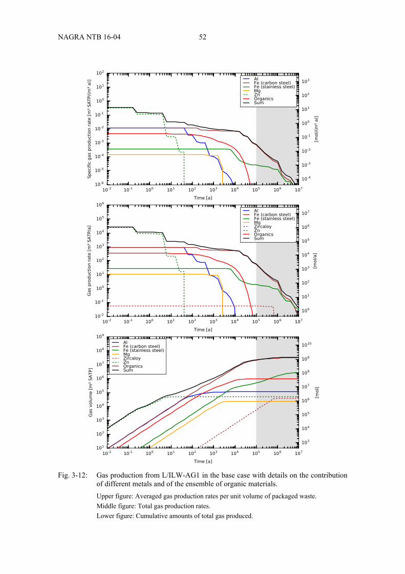
NAGRA NTB 16-04 52
Fig. 3-12: Gas production from L/ILW-AG1 in the base case with details on the contribution
of different metals and of the ensemble of organic materials. Upper figure: Averaged gas production rates per unit volume of packaged waste. Middle figure: Total gas production rates. Lower figure: Cumulative amounts of total gas produced.

53 NAGRA NTB 16-04
Fig. 3-13: Gas production from L/ILW-AG2 in the base case with details on the contribution
of different metals and of the ensemble of organic materials. Upper figure: Averaged gas production rates per unit volume of packaged waste. Middle figure: Total gas production rates. Lower figure: Cumulative amounts of total gas produced.
NAGRA NTB 16-04 54
Predominant ILW and L/ILW types
Although SF and HLW have a higher density of gas-generating materials per unit volume of packaged waste (roughly 3 × 10³ kg/m3, cf. Fig. B-1) when compared with ILW and L/ILW (on average, roughly 3 × 10² kg/m3 cf. Figs. B-2 to B-5), ILW and L/ILW will be emplaced with a much higher density of gas-generating materials (roughly two orders of magnitude higher) due to the much lower thermal power of the waste (cf. average emplacement densities in Section 2.3.1). For instance, assuming an average emplacement density of 55 m3/m (cavern type K09) results in an average L/ILW density of gas-generating material of about 1.5 × 10⁴ kg/m.30 In addition, ILW and L/ILW are more heterogeneous with respect to the amount of gas-generating materials per unit volume of packaged waste. Therefore, it is crucial to know about the waste types in ILW and L/ILW that dominate the production of gas.
Tables 3-2 and 3-3 provide information on intensely gas-producing ILW and L/ILW sorts and the most prevalent waste object in each listed waste sort. This information is extracted separately for ILW and L/ILW and irrespective of the respective waste group classification using the following methodology: The entire time frame for safety assessment is subdivided into different time periods.31 For each time period, the individual waste sorts are ranked according to the volume-specific
amount of gas produced within this time period, which is equivalent to the time-averaged volume-specific gas production rate during this period.
For each time period, it is then assumed that a single emplacement room provides a volume capacity of 10 % of the total waste volume32 of the respective waste category and that this emplacement room is theoretically filled up with waste sorts according to the ranking obtained in the previous step. In other words, the room is filled with the top-ranked waste sort; if there is space left after all this waste sort has been emplaced, then the second-ranked waste sort is emplaced and so on.
Those waste sorts that are selected for the single emplacement room are classified as "intensely gas-producing waste sorts" for the given time period. For each intensely gas-producing waste sort, the relative contribution to the total
amount of gas produced in this single emplacement room (and the given time period) is extracted.
If this relative contribution is higher than 10 %, then the waste sort is classified as a "predominant waste sort" for this time period (marked in bold).
Further, the relative contribution of the individual gas-producing object that contributes most to the gas produced by each waste sort is extracted and the corresponding waste component and the associated material are reported.
Finally, the methodology is applied to the entire time frame for safety assessment, which results in the identification of intensely gas-producing (and predominant) waste sorts from a global perspective and which are used to define the waste allocation with high gas production in a single emplacement room in an alternative case (see Section 3.1.2).
30 This may be compared with the amount of construction materials in the largest underground structure, which is
the K09 cavern and which requires as much as 2,000 kg/m of construction materials (cf. Table B-2). 31 Looking at the entire time frame is motivated by the results of gas transport modelling for the L/ILW repository
in Papafotiou & Senger (2014), which show that high gas pressure values and high gas saturation values can be expected throughout the entire time frame for safety assessment, even though maximum overpressure values occur primarily within the period between 1,000 years and 10,000 years after closure.
32 For L/ILW this amounts to 9,017 m3, which is roughly equivalent to the capacity of a single K09 cavern with 200 m length (55 m3/m × 200 m = 11,000 m3). For ILW this amounts to 393 m3, which is almost equal to the capacity of the ILW-2 tunnel (K04 cavern) with 17 m length (23 m3/m × 17 m = 391 m3).

55 NAGRA NTB 16-04
For ILW, almost all intensely gas-producing waste sorts belong to waste group AG1 (Tab. 3-2).
At early times, up until 1,000 years, the waste sort BA-PH-PF-Z3-ATA has the highest time-averaged volume-specific gas production rate in the single emplacement room. However, the waste sort SA-LU-MX-L3-SMA contributes more to the total amount of gas produced during this period – and thus to gas pressure build-up – in this room and is therefore more dominant. More generally, intensely gas-producing waste sorts are not necessarily predominant waste sorts unless they account for a major part of the waste volume in a single emplacement room. In other words, intensely gas-producing waste sorts with relatively little total volume are likely to be "diluted" by other waste sorts in the same room. In the following, the focus is on predominant waste sorts in the single emplacement room.
During the first 1,000 years, the majority of gas produced in the single emplacement room originates from the corrosion of aluminium in decommissioning waste from the Lucens reactor (SA-LU-MX-L3-SMA/ATA) and in operational waste from the surface facility of the HLW repository (BA-OH-MA-F2-SMA). A minor part results from the corrosion of carbon steel in operational waste from the PSI Hot Labor (BA-PH-PF-Z3-ATA) and in compacted hulls and ends from waste reprocessing (CSD-C, WA-F-MX-K1-ATA).
Gas production during the subsequent periods until 100,000 years is dominated by the corrosion of Mosaik-II waste containers for PWR internals (RA-G-MX-M2-SMA, RA-B-MX-M2-SMA) along with corrosion of aluminium in operational waste from the surface facility of the HLW repository, the latter with declining contributions for later time periods.
Beyond 100,000 years, gas production is dominated by the corrosion of carbon steel in decommissioning waste from the Lucens reactor (SA-LU-MX-L3-SMA), by corrosion of Zircaloy in compacted hulls and ends from waste reprocessing (CSD-C, WA-F-MX-K1-ATA) and by corrosion of stainless steel from decommissioning waste from the surface facility of the HLW repository (SA-OH-ME-F2-SMA).
Overall, gas production is dominated by the corrosion of Mosaik-II waste containers for PWR internals (RA-G-MX-M2-SMA, RA-B-MX-M2-SMA) along with corrosion of aluminium in operational waste from the surface facility of the HLW repository. The degradation of organic materials does not contribute significantly to gas production, since nearly all intensively gas-producing waste sorts belong to waste group AG1, in which organic materials play a subordinate role (cf. Fig. 3-10).
For L/ILW, intensely gas-producing waste sorts are present in both waste groups (Tab. 3-3).
At early times up until 1,000 years, gas production in the single emplacement room originates from a variety of different waste sorts and raw waste materials. However, only three waste sorts contribute more than 10 % to the total amount of gas produced within this period, all three mainly through the corrosion of carbon steel in decommissioning waste from the PSI West facilities (SA-PW-MS-C1-SMA) and in decommissioning waste from the Beznau and Leibstadt reactors (SA-L-X-F2-SMA, SA-B-X-F2-SMA). Note again that the waste sort BA-PB-X-C1-SMA, which has the highest time-averaged volume-specific gas production rate during the first sub-period, is not considered a predominant waste sort according to the adopted methodology.
Gas production during the subsequent period until 100,000 years is largely dominated by the corrosion of carbon steel in decommissioning waste from the PSI-West facilities (SA-PW-MX-C1-SMA, SA-PW-MS-C1-SMA). These are also the waste sorts that dominate gas production throughout the entire time frame for safety assessment. This result is consistent with the amounts of gas-generating materials in waste category L/ILW-AG1 (Fig. B-4).

NAGRA NTB 16-04 56
Tab. 3-2: Intensely gas-producing ILW sorts and predominant waste sorts (bold) along with the most relevant waste object within each waste sort in the base case. The methodology adopted to create the given information is explained in the main text. The nomenclature of the individual waste sorts is defined in Nagra (2014b).
Period Waste sort (percentage of gas produced in the single emplacement room)
Predominant waste object (waste component and model precursor substance, percentage)
0 a - 1,000 a
BA-PH-PF-Z3-ATA; AG2 (20.3%) C; Iron, Carbon steel (95%)
SA-LU-MX-L3-ATA; AG1 (12.7%) C; Al (99%)
SA-LU-MX-L3-SMA; AG1 (52.7%) C; Al (98%)
BA-OH-MA-F2-SMA; AG1 (7.9%) C; Al (98%)
WA-F-MX-K1-ATA; AG1 (6.5%) C; Iron, Carbon steel (75%)
1,000 a - 3,000 a
BA-OH-MA-F2-SMA; AG1 (35.6%) C; Al (99%)
RA-G-MX-M2-SMA; AG1 (35.0%) D; Iron, Carbon steel (83%)
RA-B-MX-M2-SMA; AG1 (29.4%) D; Iron, Carbon steel (83%)
3,000 a - 10,000 a
BA-OH-MA-F2-SMA; AG1 (29.8%) C; Al (98%)
RA-G-MX-M2-SMA; AG1 (38.1%) D; Iron, Carbon steel (94%)
RA-B-MX-M2-SMA; AG1 (32.1%) D; Iron, Carbon steel (94%)
10,000 a - 30,000 a
RA-G-MX-M2-SMA; AG1 (44.9%) D; Iron, Carbon steel (96%)
RA-B-MX-M2-SMA; AG1 (53.2%) D; Iron, Carbon steel (96%)
BA-OH-MA-F2-SMA; AG1 (1.9%) C; Al (91%)
30,000 a - 100,000 a
RA-G-MX-M2-SMA; AG1 (43.9%) D; Iron, Carbon steel (98%)
RA-B-MX-M2-SMA; AG1 (52.0%) D; Iron, Carbon steel (98%)
BA-PB-X-Z1-ATA; AG1 (4.0%) D; Iron, Carbon steel (54%)
100,000 a - 300,000 a SA-LU-MX-L3-SMA; AG1 (44.8%) C; Iron, Carbon steel (88%)
WA-F-MX-K1-ATA; AG1 (55.2%) C; Zircaloy (92%)
300,000 a - 1,000,000 a
SA-OH-ME-F2-SMA; AG1 (41.0%) C; Stainless steel, Ni-alloys (100%)
SA-LU-MX-L3-SMA; AG1 (41.2%) C; Iron, Carbon steel (91%)
BA-PW-MX-C1-ATA; AG1 (5.6%) F; Iron, Carbon steel (51%)
SA-LU-MX-L3-ATA; AG1 (4.5%) C; Iron, Carbon steel (85%)
BA-PH-PL-Z3-ATA; AG1 (2.9%) D; Stainless steel, Ni-alloys (100%)
BA-OH-MS-F2-SMA; AG1 (4.8%) C; Iron, Carbon steel (100%)
0 a - 1,000,000 a
RA-G-MX-M2-SMA; AG1 (44.2%) D; Iron, Carbon steel (95%)
RA-B-MX-M2-SMA; AG1 (52.3%) D; Iron, Carbon steel (95%)
BA-OH-MA-F2-SMA; AG1 (3.5%) C; Al (92%)

57 NAGRA NTB 16-04
Tab. 3-3: Intensely gas-producing L/ILW sorts and predominant waste sorts (bold) along with the most relevant waste object in each waste sort in the base case. The methodology adopted to create the given information is explained in the main text. The nomenclature of the individual waste sorts is defined in Nagra (2014b).
Note that the present analysis uses the MIRAM 14 base scenario and not the updated PSI-West inventory.
Period Waste sort (percentage of gas produced in the single emplacement room)
Predominant waste object (waste component and model precursor substance, percentage)
0 a - 1,000 a
BA-PB-X-C1-SMA; AG1 (1.4%) C; Mg (100%)
SA-PD-X-C1-SMA; AG2 (7.6%) C; Iron, Carbon steel (88%)
BA-PB-X-Z1-SMA; AG2 (5.9%) D; Iron, Carbon steel (51%)
SA-P-MA-C1-SMA; AG2 (0.9%) C; Al (85%)
BA-C-MA-C1-SMA; AG2 (7.6%) C; Al (85%)
SA-PW-MA-C1-SMA; AG2 (0.2%) C; Al (83%)
SA-PD-MA-C1-SMA; AG2 (0.2%) C; Al (84%)
SA-B-MS-M2-SMA; AG1 (0.6%) C; Iron, Carbon steel (84%)
SA-Z-X-F2-SMA; AG2 (0.1%) C; Iron, Carbon steel (69%)
BA-G-F-F2-SMA; AG1 (0.9%) C; Iron, Carbon steel (86%)
SA-PD-MS-C1-SMA; AG1 (0.2%) C; Al (98%)
SA-PP-X-C1-SMA; AG1 (0.2%) C; Mg (90%)
SA-M-X-F2-SMA; AG2 (4.7%) C; Iron, Carbon steel (59%)
SA-L-X-F2-SMA; AG2 (16.0%) C; Iron, Carbon steel (56%)
SA-G-X-F2-SMA; AG2 (9.0%) C; Iron, Carbon steel (57%)
SA-PD-X-F2-SMA; AG1 (0.1%) C; Al (93%)
SA-PS-X-C1-SMA; AG2 (0.6%) C; Iron, Carbon steel (64%)
SA-B-X-F2-SMA; AG2 (11.8%) C; Iron, Carbon steel (53%)
SA-PW-MS-C1-SMA; AG1 (28.8%) C; Iron, Carbon steel (96%)
BA-M-X-F2-SMA; AG2 (3.3%) C; Iron, Carbon steel (67%)
1,000 a - 3,000 a
BA-PB-X-C1-SMA; AG1 (1.4%) C; Mg (100%)
BA-C-MA-C1-SMA; AG2 (8.6%) C; Al (94%)
SA-P-MA-C1-SMA; AG2 (1.0%) C; Al (94%)
SA-PW-MA-C1-SMA; AG2 (0.2%) C; Al (94%)
SA-PD-MA-C1-SMA; AG2 (0.2%) C; Al (94%)
SA-PW-MS-C1-SMA; AG1 (43.6%) C; Iron, Carbon steel (99%)
SA-PW-MX-C1-SMA; AG1 (45.0%) C; Iron, Carbon steel (99%)

NAGRA NTB 16-04 58
Tab. 3-3: (continued)
Period Waste sort (percentage of gas produced in the single emplacement room)
Predominant waste object (waste component and model precursor substance, percentage)
3,000 a - 10,000 a
SA-PW-MS-C1-SMA; AG1 (49.0%) C; Iron, Carbon steel (100%)
BA-C-MA-C1-SMA; AG2 (4.1%) C; Al (100%)
SA-PW-MA-C1-SMA; AG2 (0.1%) C; Al (100%)
SA-PD-MA-C1-SMA; AG2 (0.1%) C; Al (100%)
SA-P-MA-C1-SMA; AG2 (0.4%) C; Al (100%)
SA-PW-MX-C1-SMA; AG1 (46.3%) C; Iron, Carbon steel (99%)
10,000 a - 30,000 a
SA-PW-MS-C1-SMA; AG1 (51.9%) C; Iron, Carbon steel (100%)
SA-PW-MX-C1-SMA; AG1 (47.8%) C; Iron, Carbon steel (99%)
SA-PS-MX-M2-SMA; AG1 (0.03%) D; Iron, Carbon steel (95%)
SA-B-H-M2-SMA; AG2 (0.3%) D; Iron, Carbon steel (95%)
30,000 a - 100,000 a
SA-PW-MX-C1-SMA; AG1 (73.9%) C; Iron, Carbon steel (97%)
SA-PP-X-C1-SMA; AG1 (0.2%) C; Iron, Carbon steel (96%)
BA-C-MS-C1-SMA; AG1 (7.2%) C; Iron, Carbon steel (96%)
SA-L-ME-M2-SMA; AG1 (6.7%) D; Iron, Carbon steel (93%)
SA-G-ME-M2-SMA; AG1 (4.9%) D; Iron, Carbon steel (93%)
SA-PD-X-C1-SMA; AG2 (2.1%) C; Iron, Carbon steel (100%)
SA-M-ME-M2-SMA; AG1 (4.7%) D; Iron, Carbon steel (95%)
SA-B-ME-M2-SMA; AG1 (0.4%) D; Iron, Carbon steel (95%)
0 a - 100,000 a
SA-PW-MS-C1-SMA; AG1 (43.5%) C; Iron, Carbon steel (99%)
SA-PW-MX-C1-SMA; AG1 (56.2%) C; Iron, Carbon steel (98%)
SA-B-MS-M2-SMA; AG1 (0.3%) D; Iron, Carbon steel (88%)
SA-PS-MX-M2-SMA; AG1 (0.03%) D; Iron, Carbon steel (91%)
SA-B-H-M2-SMA; AG2 (0.03%) D; Iron, Carbon steel (92%)
It should be noted that the present analysis uses the MIRAM 14 base scenario; for the alternative scenario with the updated PSI-West inventory it is inferred that decommissioning waste from the PSI-West research facility will be less dominant.
The degradation of organic materials does not contribute significantly to gas production.

59 NAGRA NTB 16-04
3.1.2 Uncertainties
This section explores the impact of relevant uncertainties starting from the base case. According to Table 2-3, the key uncertainties for waste and disposal containers are corrosion rates, degradation rates for ILW and L/ILW, the local influence of degradation of organic materials on corrosion for ILW and L/ILW, as well as the location of specific ILW and L/ILW in the repositories. As mentioned earlier, only the net results for gas production rates and amounts of produced gas are reported in the following paragraphs.
Corrosion rates
Figs. 3-14 to 3-16 show averaged volume-specific gas production rates, total gas production rates and total cumulative amounts of produced gas for the respective base cases, and compares these with alternative cases that assume upper and lower bound corrosion rates. Note that the variation is concordant with respect to the different metals, i.e. there is no combination of high corrosion rates for one metal with low corrosion rates for another metal.
The following observations can be made:
Prior to canister breaching, which is assumed to occur at the reference lifetime of 10,000 years for both the SF and the HLW disposal canisters, the gas production rate assuming the upper bound corrosion rates is a factor of around 2.5 higher than in the base case. The gas production rate assuming the lower bound corrosion rates is a factor of around 20 lower than in the base case. These differences in gas production reflect the differences in the corrosion rate for "Iron, Carbon steel: anaerobic corrosion", which is the single model precursor substance for the disposal canister walls. Once the disposal canister is breached, water reaches the interior of the canister and corrosion processes start to occur at the inner surface of the disposal canister and at the surface of the waste. The gas production rate for SF and HLW then shows a marked sensitivity to the corrosion rates. If the upper bound corrosion rates are assumed, the peak that occurs upon canister breaching is higher but of shorter duration than that of the base case, with the gas production rate dropping below that of the base case some 20,000 years post closure, once corrosion of the canister has ended. If the lower bound corrosion rates are assumed, the peak that occurs upon canister breaching is, conversely, lower and of longer duration than that of the base case. Assuming these lower bound rates, the gas production rate does not fall significantly for some hundreds of thousands of years, reflecting the long duration of canister corrosion in this case. The total amounts of gas produced after a million years are 2.2 × 10⁷ m3 (SATP) for SF and 1.2 × 10⁶ m3 (SATP) for HLW, irrespective of the corrosion rates assumed.
The sensitivity of gas production rates for ILW to corrosion rates is more complex. Although, in general, gas production rates are higher than the base case if upper bound corrosion rates are assumed, with the converse being true of lower bound rates, this is not the case at all times. There are, for example, several relatively short duration periods when the base case gas generation rate is higher than that calculated assuming the upper bound corrosion rates. This is due to the more rapid depletion of certain components if high corrosion rates are assumed. The total amounts of gas produced for ILW after a million years are almost identical in the base case and in the case assuming the upper bound corrosion rates. For the lower bound corrosion rates, significant gas production continues beyond a million years; it takes a few million years before the total amount of gas produced reaches a constant value that is the same as that calculated in the higher corrosion rate cases.

NAGRA NTB 16-04 60
Similar observations to those for ILW can be made for L/ILW. In general, gas production rates are higher than those of the base case if upper bound corrosion rates are assumed, with the converse being true of lower bound rates, but there are some periods when this is not the case. The total amounts of gas produced for L/ILW after one hundred thousand years are almost identical in the base case and in the case assuming the upper bound corrosion rates, although the total amount of gas produced for L/ILW-AG1 is still increasing at this time. For the lower bound corrosion rates, significant gas production continues beyond one hundred thousand years. It takes around a million years before the total amount of gas produced for L/ILW-AG2 reaches a constant value that is the same as that calculated in the higher corrosion rate cases. The corresponding time for L/ILW-AG1 is several million years.

61 NAGRA NTB 16-04
Fig. 3-14: Gas production from SF and HLW for the base cases and for alternative cases with
upper and lower bound corrosion rates. Upper figure: Averaged gas production rates per unit volume of packaged waste. Middle figure: Total gas production rates. Lower figure: Cumulative amounts of total gas produced.

NAGRA NTB 16-04 62
Fig. 3-15: Gas production from ILW-AG1 and ILW-AG2 for the base cases and for
alternative cases with upper and lower bound corrosion rates. Upper figure: Averaged gas production rates per unit volume of packaged waste. Middle figure: Total gas production rates. Lower figure: Cumulative amounts of total gas produced.

63 NAGRA NTB 16-04
Fig. 3-16: Gas production from L/ILW-AG1 and L/ILW-AG2 for the base cases and for
alternative cases with upper and lower bound corrosion rates. Upper figure: Averaged gas production rates per unit volume of packaged waste. Middle figure: Total gas production rates. Lower figure: Cumulative amounts of total gas produced.

NAGRA NTB 16-04 64
Degradation rates for ILW and L/ILW
Figs. 3-17 and 3-18 show averaged volume-specific gas production rates, total gas production rates and total cumulative amounts of gas produced from ILW and L/ILW for the respective base cases and compares these with alternative cases with upper bound and lower bound, i.e. zero, degradation rates. Note that the variation is concordant with respect to the different groups of organic materials, i.e. there is no combination of high degradation rates for one group with low degradation rates for the other group.
The following observations can be made:
Gas production for ILW-AG1 shows hardly any sensitivity to degradation rates across the range of values investigated, reflecting the dominance of hydrogen generation from metal corrosion. For ILW-AG2, gas production rates based on upper bound degradation rates are similar to those of the base case, except during the period from around 0.2 years to around 200 years, when they are higher than the base-case rates, and from around 2,000 years to 20,000 years, when they are lower. Gas production rates based on lower bound degradation rates are similar to those of the base case, except during the period from around 200 years to around 20,000 years (and especially during the earlier part of this period), when they are substantially lower.33 Recall that, between about 200 and 3,000 years, methane from the degradation of various organic substances is the main species of net gas produced for ILW-AG2 in the base case and would thus be expected to be sensitive to the assumed degradation rates, and that the production of methane starts to decline significantly at about 10,000 years.
The total amounts of gas produced after a million years for ILW are virtually independent of the degradation rates assumed.
For L/ILW-AG1, gas production rates – if upper bound degradation rates are assumed – are similar to those of the base case given the bias inherent in the base case, except during the period from around 5 years to around 2,000 years, when they are higher than the base-case rates. Gas production rates based on lower bound degradation rates are slightly lower during this period, but the difference compared with the base case is relatively small. For L/ILW-AG2, gas production rates based on upper bound degradation rates are higher than those of the base case for the period up to around 2,000 years, and then lower up to around 40,000 years. Thereafter, they are similar. Gas production rates based on lower bound degradation rates are similar to those of the base case up to around 200 years. From 200 years to around 40,000 years, the gas production rates are lower than in the base case, but are similar thereafter. Recall that, for L/ILW-AG2, a significant decline in hydrogen production occurs after a few hundred years, allowing methane and carbon dioxide production to become similar to that of hydrogen for some tens of thousands of years, explaining the sensitivity to a reduction in degradation rates during this period.
The total amounts of gas produced for L/ILW after one hundred thousand years are almost identical for the base case and for the case assuming the upper bound degradation rates, although the total amount of gas produced for L/ILW-AG1 is still increasing at this time. For the lower bound degradation rates, the total amount of gas produced for L/ILW-AG2 reaches a constant value at around one 100,000 years, but the value calculated for the base case and for the upper bound degradation rate is higher than that for the lower bound degradation rates since no degradation is assumed in the latter case.
33 Of course, the gas production rate for this case is always equal to, or lower than, the rate for the other cases due to
the lower bounding assumption of no degradation.

65 NAGRA NTB 16-04
Fig. 3-17: Gas production from ILW-AG1 and ILW-AG2 for the base cases and for
alternative cases with upper and lower bound degradation rates. Upper figure: Averaged gas production rates per unit volume of packaged waste. Middle figure: Total gas production rates. Lower figure: Cumulative amounts of total gas produced.

NAGRA NTB 16-04 66
Fig. 3-18: Gas production from L/ILW-AG1 and L/ILW-AG2 for the base cases and for
alternative cases with upper and lower bound degradation rates. Upper figure: Averaged gas production rates per unit volume of packaged waste. Middle figure: Total gas production rates. Lower figure: Cumulative amounts of total gas produced.

67 NAGRA NTB 16-04
Local influence of degradation on corrosion for ILW and L/ILW
In the base case, it is hypothetically assumed that complete and instant degradation of organic materials leads to local heterogeneities in environmental conditions and specifically to a local lowering of pH, with a consequent increase in corrosion rates (see Section 2.1). Figs. 3-19 and 3-20 show averaged volume-specific gas production rates, total gas production rates and total cumulative amounts of gas produced from ILW and L/ILW for the respective base cases and for alternative cases with no pH change due to the degradation of organic materials.
The following observations can be made:
Gas production for ILW shows some sensitivity to pH change from early times: around a year for ILW-AG1 and well under a year for ILW-AG2.
The assumption of no pH change due to the degradation of organic materials results in generally lower gas production rates for ILW-AG1 for up to some tens of thousands of years.
This assumption also leads to lower gas production rates for ILW-AG2, but only up to around 200 to 300 years. Recall that, in the base case, hydrogen production due to corrosion starts to decrease very early, at about 200 years, for this waste category and that, between about 200 and 3,000 years, methane from the degradation of various organic substances is the main species of net gas produced. These would not be affected by the assumptions made regarding pH change.
The total amounts of gas produced after a million years for ILW are virtually independent of the assumptions made regarding pH change, especially in the case of ILW-AG2.
Gas production for L/ILW-AG1 shows little sensitivity to pH change at any time.
The assumption of no pH change due to the degradation of organic materials results in generally lower gas production rates for L/ILW-AG2, especially in the period up to around 2,000 years, after which hydrogen production due to corrosion becomes less significant compared with carbon dioxide and methane production (see Fig. 3-6).
The total amounts of gas produced for L/ILW-AG1 after one hundred thousand years are almost identical for the base case and for the case assuming no pH change due to the degradation of organic materials, with the total amount of gas produced still increasing at this time in both cases. For L/ILW-AG2, the total amount of gas produced reaches a constant value at around 100,000 years in the base case, but only reaches this same value after several hundred thousand years in the case assuming no pH change due to the degradation of organic materials.

NAGRA NTB 16-04 68
Fig. 3-19: Gas production from ILW-AG1 and ILW-AG2 for the base cases and for
alternative cases with no pH change due to the degradation of organic materials. Upper figure: Averaged gas production rates per unit volume of packaged waste. Middle figure: Total gas production rates. Lower figure: Cumulative amounts of total gas produced.

69 NAGRA NTB 16-04
Fig. 3-20: Gas production from L/ILW-AG1 and L/ILW-AG2 for the base cases and for
alternative cases with no pH change due to the degradation of organic materials. Upper figure: Averaged gas production rates per unit volume of packaged waste. Middle figure: Total gas production rates. Lower figure: Cumulative amounts of total gas produced.
NAGRA NTB 16-04 70
Location of ILW and L/ILW in the repositories
Waste types that are comparatively intensive with respect to the production of gas are identified in Section 3.1.1. In the base case, it is implicitly assumed that the waste and above all the intensely gas-producing waste types are distributed uniformly across the individual emplace-ment rooms for the respective waste categories.
Figs. 3-21 and 3-22 show averaged volume-specific gas production rates, total gas production rates and total cumulative amounts of gas produced from ILW and L/ILW for the base cases of the different waste groups, and compares these with alternative cases, in which the intensely gas-producing waste types for ILW and L/ILW (results from Tables 3-2 and 3-3 based on the entire time frame for safety assessment) are allocated to a single emplacement room, the remainder of the waste being distributed uniformly across the remaining emplacement rooms (without distinction of waste groups).
The figures also show the results for another alternative case, in which the most weakly gas-producing waste types for ILW and L/ILW are allocated to a single emplacement room based on the same methodology used for the identification of intensely gas-producing waste types. The remainder of the waste is again distributed uniformly across the remaining emplacement rooms (without distinction of waste groups).
The following observations can be made:
For ILW, the specific gas production rates are generally higher in a single room filled with the most intensely gas-producing waste types than in a single room filled with the least intensely gas-producing waste types, as identified by the applied methodology, except at early times (less than around 1,000 years) and late times (greater than around 100,000 years), when the rates are lower because the gas-producing material is consumed. The reason why at early times the gas production for the single room is lower than that of the base case (and the remaining rooms) is that gas production for the entire time period is dominated by Mosaik-II waste containers for PWR internals, which have their most dominant period between 1,000 and 100,000 years (cf. Table 3-2).
The specific gas production rate for ILW in a single room filled with the most intensely gas-producing waste types exceeds the average specific gas production rate in all other rooms in the period between a few hundred years and a few tens of thousands of years.
The total gas production rates are also generally higher in a single room filled with the most intensely gas-producing waste types than in a single room filled with the least intensely gas-producing waste types, except at similarly early times for the reasons described above. At late times, the gas production rates of the single rooms are similar, irrespective of waste type allocation.
The total gas production rate for ILW in a single room filled with the most intensely gas-producing waste types also exceeds the combined gas production rates in all other rooms, but for a shorter period starting at around 20,000 years and persisting for another couple of tens of thousands of years.
The total amount of gas produced after a million years for ILW in a single room filled with the most intensely gas-producing waste is around 3 × 10⁵ m3 (SATP) and around 2 × 10⁴ m3 (SATP) in a single room filled with the least intensely gas-producing waste. The corre-spondding values for all other rooms are in the order of 106 m3 (SATP).
For L/ILW, the specific and total gas production rates are higher in a single room filled with the most intensely gas-producing waste types than in a single room filled with the most weakly gas-producing waste types at all times.

71 NAGRA NTB 16-04
Fig. 3-21: Gas production from ILW for the base cases and for alternative cases with waste
allocations to a single emplacement room with high and low gas production. Upper figure: Averaged gas production rates per unit volume of packaged waste. Middle figure: Total gas production rates. Lower figure: Cumulative amounts of total gas produced.
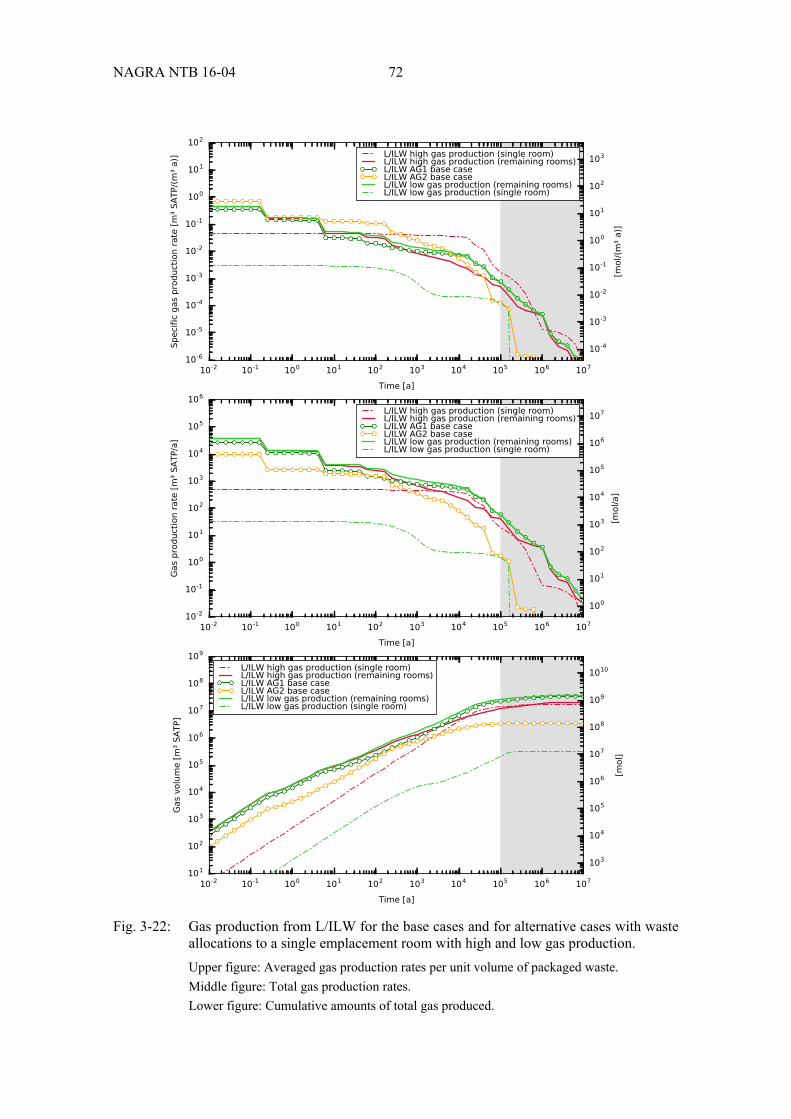
NAGRA NTB 16-04 72
Fig. 3-22: Gas production from L/ILW for the base cases and for alternative cases with waste
allocations to a single emplacement room with high and low gas production. Upper figure: Averaged gas production rates per unit volume of packaged waste. Middle figure: Total gas production rates. Lower figure: Cumulative amounts of total gas produced.

73 NAGRA NTB 16-04
The specific gas production rate for L/ILW in a single room filled with the most intensely gas-producing waste types exceeds the average specific gas production rate in all other rooms at times beyond a few tens of years.
The total gas production rate for L/ILW in a single room filled with the most intensely gas-producing waste types is quite similar to the combined gas production rates in all other rooms at times beyond around 1,000 years, but is less than the combined gas production rates in all other rooms at earlier times.
The total amount of gas produced after one hundred thousand years for L/ILW in a single room filled with the most intensely gas-producing waste is around 2 × 10⁷ m3 (SATP), and is rather similar to the total amount of gas produced in all other rooms combined. The corresponding values for a single room filled with the least intensely gas-producing waste are around 3 × 10⁵ m3 (SATP).

NAGRA NTB 16-04 74
3.1.3 Options
This section explores the potential impact of relevant options that exist for the waste and the disposal containers starting from the base case. According to Table 2-3, these options are (i) the removal / replacement of ILW and L/ILW containment prior to packaging in disposal con-tainers, (ii) the pyrolysis and/or melting of ILW and L/ILW and (iii) the use of an alternative disposal canister for SF and HLW. As mentioned earlier, only the net results for gas production rates and amounts of produced gas are reported in the following paragraphs.
Removal / replacement of ILW and L/ILW containment
In the base case, it is assumed that the waste is emplaced as it is conditioned today and presumably in the future. Figs. 3-23 to 3-26 show averaged volume-specific gas production rates, total gas production rates and total cumulative amounts of gas produced from the different ILW and L/ILW waste categories for the base case and for alternative cases, in which it is assumed that all drums are removed and/or Mosaik-II waste containers are replaced prior to packaging in disposal containers.
The following observations can be made:
For ILW-AG1, removal of the drums makes very little difference to either the gas production rates or the total cumulative amounts of gas produced. However, replacement of Mosaik-II waste containers by alternative disposal containers that do not significantly produce gas leads to lower gas production rates between a few hundred years and a few tens of thousands of years. The total amount of gas produced after a million years for ILW-AG1 with Mosaik-II waste containers removed is slightly less than in the base case or in the case in which only drums are removed.
For ILW-AG2, replacement of Mosaik-II waste containers by alternative disposal containers that do not significantly produce gas makes very little difference to either the gas production rates or the total cumulative amounts of gas produced. However, removal of the drums leads to lower gas production rates for a few months and then again from between around 20,000 years and a million years. The total amount of gas produced after a million years for ILW-AG2 with the drums removed is slightly less than in the base case or in the case in which only Mosaik-II waste containers are removed.
For L/ILW-AG1, replacement of Mosaik-II waste containers by alternative disposal containers that do not significantly produce gas makes very little difference to either the gas production rates or the total cumulative amounts of gas produced. However, removal of the drums leads to lower gas production rates for the first few months and then again from around 20,000 to 30,000 years. The total amount of gas produced after one hundred thousand years is similar in all cases considered for L/ILW-AG1.
For L/ILW-AG2, replacement of Mosaik-II waste containers by alternative disposal containers that do not significantly produce gas leads to lower gas production rates between around 10,000 years and 70,000 years. Removal of the drums leads to lower gas production rates for the first few months and then again from around 200 to 300 years and finally between around 50,000 years and the end of the calculation. The total amount of gas produced after one hundred thousand years for L/ILW-AG2 in cases with the drums removed and Mosaik-II waste containers replaced by alternative disposal containers that do not produce gas is slightly less than in the base case.

75 NAGRA NTB 16-04
Fig. 3-23: Gas production from ILW-AG1 for the base case and for alternative cases in which
all drums are removed and/or Mosaik-II waste containers are replaced. Upper figure: Averaged gas production rates per unit volume of packaged waste. Middle figure: Total gas production rates. Lower figure: Cumulative amounts of total gas produced.

NAGRA NTB 16-04 76
Fig. 3-24: Gas production from ILW-AG2 for the base case and for alternative cases in which
all drums are removed and/or Mosaik-II waste containers are replaced. Upper figure: Averaged gas production rates per unit volume of packaged waste. Middle figure: Total gas production rates. Lower figure: Cumulative amounts of total gas produced.

77 NAGRA NTB 16-04
Fig. 3-25: Gas production from L/ILW-AG1 for the base case and for alternative cases in
which all drums are removed and/or Mosaik-II waste containers are replaced. Upper figure: Averaged gas production rates per unit volume of packaged waste. Middle figure: Total gas production rates. Lower figure: Cumulative amounts of total gas produced.

NAGRA NTB 16-04 78
Fig. 3-26: Gas production from L/ILW-AG2 for the base case and for alternative cases in
which all drums are removed and Mosaik-II waste containers are replaced. Upper figure: Averaged gas production rates per unit volume of packaged waste. Middle figure: Total gas production rates. Lower figure: Cumulative amounts of total gas produced.

79 NAGRA NTB 16-04
Pyrolysis and melting of ILW and L/ILW (base scenario and alternative scenario with updated PSI-West inventory)
The base case reflects the base scenario of the modelled waste inventory MIRAM 14 (Nagra 2014b) and the corresponding waste allocation to the different repository types in Nagra (2014d). In order to show the impact of currently available processes capable of reducing and / or avoiding organic and metallic materials in ILW and L/ILW, the following alternative waste scenarios are analysed:
Pyrolysis (M14AP, realistic scenario)
Total pyrolysis (M14APA, hypothetical scenario)
Melting (M14AS, realistic scenario)
Pyrolysis and melting (combination of M14AP and M14AS, realistic scenario)
As mentioned in Section 2.3.1, recent analyses have also led to an update of the inventory of decommissioning waste from the PSI-West research facility. Therefore, the following additional alternative waste scenarios are analysed and the results are compared to the MIRAM 14 base scenario and the associated alternative scenarios (see above):
Updated PSI-West inventory (M14A U PSIW, realistic scenario)
Updated PSI-West inventory and melting (M14AS U PSIW, realistic scenario)
A detailed description of all alternative waste scenarios can be found in Stein (2016). The total amounts of gas-generating materials per model precursor substance are illustrated for each alternative waste scenario in Section B.1.2. Further details can also be found in the respective gas generation tools (cf. Section 2.4).
Waste sorts of the base scenario that are subject to waste treatment in the different alternative waste scenarios are listed in Table 3-4 for the individual waste categories ILW-AG1, ILW-AG2, L/ILW-AG1, L/ILW-AG2. Those waste sorts that have been identified as intensely gas-producing for any time period (cf. Tables 3-2 and 3-3) are marked in bold. Note that from a given waste sort, not all waste packages are necessarily subject to waste treatment (cf. Stein 2016).
In the case of ILW the number of treated waste sorts is small and the associated packaged volume is at most as high as 713 m3, which is roughly 18 % of the total ILW volume. In addition, only a few waste sorts that are subject to treatment in the melting scenario have also been identified as intensely gas-producing waste sorts in Section 3.1.1 (cf. Table 3-2); the overall effect of waste treatment on gas generation in the ILW part of the HLW repository is thus expected to be minor.
In the case of L/ILW, the number of treated waste sorts ranges from 8 in the realistic pyrolysis scenario to 31 in the hypothetical total pyrolysis scenario. The corresponding volume of treated waste ranges from about 5,600 m3 to about 24,700 m3, the latter reflecting about 27 % of the total packaged waste volume in the L/ILW repository. As for ILW, only a few waste sorts that are subject to treatment in the individual scenarios have also been identified as intensely gas-producing in Section 3.1.1 (cf. Table 3-3). However, the treated waste sorts in the melting scenarios include those from the PSI West facilities (SA-PW-MX-C1-SMA, SA-PW-MS-C1-SMA), which have been classified as predominant waste types in the base scenario. Therefore, a perceptible effect of melting on gas generation in the L/ILW repository is expected if the base scenario is assumed.

NAGRA NTB 16-04 80
Tab. 3-4: Waste sorts in the ILW and L/ILW repository that are subject to waste treatment options and waste volumes involved for different alternative waste scenarios. Bold: Intensely gas-producing waste sorts according to Tables 3-2 and 3-3.
Scenario Pyrolysis Total pyrolysis Melting Pyrolysis and
melting
Total volume of ILW prior to treatment [m3]
3,932
ILW-AG1 BA-OH-H-F2-SMA
BA-OH-H-F2-SMA BA-OH-MA-F2-SMA
BA-OH-ME-F2-SMA BA-OH-MS-F2-SMA SA-OH-ME-F2-SMA
BA-OH-H-F2-SMA BA-OH-MA-F2-
SMA BA-OH-ME-F2-SMA BA-OH-MS-F2-SMA SA-OH-ME-F2-SMA
ILW-AG2 - - - -
Total volume of treated ILW [m3]
221 221 492 713
Total volume of L/ILW prior to treatment [m3]
90,172
L/ILW-AG1 BA-L-H-F2-SMA BA-M-H-F2-SMA
BA-B-K-B1-SMA BA-B-K-F2-SMA BA-C-X-C1-SMA BA-G-H-F2-SMA
BA-G-HB-B1-SMA BA-L-H-F2-SMA BA-M-H-F2-SMA
BA-PV-AF-F2-SMA SA-B-K-F2-SMA
SA-B-MS-L3-SMA SA-B-MS-M2-SMA
SA-G-K-F2-SMA SA-G-MS-L3-SMA SA-L-K-F2-SMA
SA-L-MS-L3-SMA SA-M-K-F2-SMA
SA-M-MX-L3-SMA SA-Z-K-F2-SMA
BA-C-MX-C1-SMA SA-B-MS-L3-SMA SA-B-MX-F2-SMA SA-B-MX-L3-SMA SA-G-ME-L3-SMA SA-G-MS-L3-SMA SA-G-MX-L3-SMA SA-L-ME-L3-SMA SA-L-MS-L3-SMA SA-L-MX-F2-SMA SA-L-MX-L3-SMA SA-M-ME-L3-SMA SA-M-MS-L3-SMA SA-M-MX-F2-SMA SA-M-MX-L3-SMA
SA-PW-MC-C1-SMA SA-PW-ME-C1-SMA
SA-PW-MS-C1-SMA
SA-PW-MX-C1-SMA
BA-C-MX-C1-SMA BA-L-H-F2-SMA BA-M-H-F2-SMA SA-B-MS-L3-SMA SA-B-MX-F2-SMA SA-B-MX-L3-SMA SA-G-ME-L3-SMA SA-G-MS-L3-SMA SA-G-MX-L3-SMA SA-L-ME-L3-SMA SA-L-MS-L3-SMA SA-L-MX-F2-SMA SA-L-MX-L3-SMA SA-M-ME-L3-SMA SA-M-MS-L3-SMA SA-M-MX-F2-SMA SA-M-MX-L3-SMA
SA-PW-MC-C1-SMA SA-PW-ME-C1-SMA
SA-PW-MS-C1-SMA
SA-PW-MX-C1-SMA

81 NAGRA NTB 16-04
Tab. 3-4: (continued) Bold: Intensely gas-producing waste sorts according to Tables 3-2 and 3-3.
Scenario Pyrolysis Total pyrolysis Melting Pyrolysis and
melting
L/ILW-AG2 BA-B-HP-F2-SMA BA-G-HB-F2-
SMA SA-B-H-M2-SMA SA-G-H-M2-SMA SA-L-H-M2-SMA SA-M-H-M2-SMA
BA-B-HP-F1-SMA BA-B-HP-F2-SMA BA-G-HB-F2-SMA BA-G-KB-B1-SMA BA-G-KB-F2-SMA SA-B-H-M2-SMA SA-B-X-F2-SMA SA-G-H-M2-SMA SA-G-X-F2-SMA SA-L-H-M2-SMA SA-L-X-F2-SMA SA-M-H-M2-SMA SA-M-X-F2-SMA
BA-B-HP-F2-SMA BA-G-HB-F2-SMA SA-B-H-M2-SMA SA-G-H-M2-SMA SA-L-H-M2-SMA SA-M-H-M2-SMA
Total volume of treated L/ILW [m3]
5,639 24,018 19,070 24,709
The output of the different waste treatment processes is new waste that contains (part of) the treated waste, as well as secondary waste from the melting and pyrolysis facilities.34 Part of this new waste belongs to existing waste sorts and the other part is specified in new waste sorts. For simplicity, the new waste that belongs to existing waste sorts inherits the original attributes (repository allocation, affiliation with one of the two waste groups, classification according to the potential maximum reduction in pH).
All new waste sorts represent low- and intermediate-level waste without excessive amounts of alpha-emitting radionuclides (cf. Stein 2016). It is therefore assumed for the sake of simplicity that all of these new waste sorts are allocated to the L/ILW repository.35 Also for the sake of simplicity, no distinction of waste groups is made for the L/ILW repository. The classification of the new waste sorts according to their content of organic material and the resulting potential maximum reduction in pH is carried out using the standard methodology developed in Cloet et al. (2014).36
Table 3-5 provides information about new waste that results from waste treatment processes and the volumes involved. New waste sorts cover by far the largest part of the new waste. The total volume of new waste ranges from about 2,900 m3 in the pyrolysis scenario to about 20,100 m3 34 Assumptions: The metal ingots resulting from the melting process are conditioned into LC-84 containers. The
secondary waste from the melting facility is packaged into KC-T12 containers and the secondary waste from the pyrolysis facility is conditioned in 200 litre drums. These drums are then packaged in LC-84H disposal containers in the surface facility of the repository; here the same assumptions with regard to packaging are made as for similar waste packages in the base scenario.
35 It should be noted that the way existing and new waste sorts are allocated to the different repository types in this study is rather stylised and not conform to the method adopted in the site selection process (cf. Nagra 2014d). The simplified approach adopted here is however justified by the fact that the expected effects of waste treatment on gas production in the ILW part of the HLW repository are small and that the adopted approach tends to overestimate gas production in the L/ILW repository.
36 Note that some of the residues of the pyrolysis process are attributed to the model precursor substance "Asche" (ash), for which it is assumed that only 5 wt-% contribute to gas production.

NAGRA NTB 16-04 82
in the combined pyrolysis and melting scenario, the latter reflecting about 22 % of the original total waste volume in the L/ILW repository. The resulting total volume in the L/ILW repository and the required number of L/ILW emplacement rooms are not very different from the original situation; however the hypothetical total pyrolysis scenario leads to a marked reduction in total volume, which should in turn have a discernible effect on the averaged volume-specific gas production rate.
Tab. 3-5: Waste in the L/ILW repository resulting from waste treatment options and waste volumes for different alternative waste scenarios. Bold: Intensely gas-producing waste sorts according to Table 3-3.
Scenario Pyrolysis Total pyrolysis Melting Pyrolysis and melting
Existing waste sorts
BA-PB-X-Z1-SMA SA-L-K-F2-SMA
SA-PW-B-C1-SMA SA-L-K-F2-SMA SA-PW-B-C1-SMA
New waste sorts
BA-B-AP-M2-SMA BA-G-AP-M2-SMA BA-L-AP-M2-SMA BA-L-K-F2-SMA BA-M-AP-M2-
SMA BA-OH-AP-M2-
SMA SA-B-AP-M2-SMA SA-G-AP-M2-SMA SA-L-AP-M2-SMA SA-M-AP-M2-SMA
BA-OH-AP-M2-SMA
BA-OH-SM-F2-SMA
SA-B-IN-L3-SMA SA-B-SM-F2-SMA SA-C-IN-L3-SMA SA-G-IN-L3-SMA SA-G-SM-F2-SMA SA-L-IN-L3-SMA SA-L-SM-F2-SMA SA-M-IN-L3-SMA SA-M-SM-F2-SMA
SA-OH-IN-L3-SMA
SA-OH-SM-F2-SMA
SA-PW-IN-L3-SMA
BA-B-AP-M2-SMA BA-G-AP-M2-SMA BA-L-AP-M2-SMA BA-L-K-F2-SMA
BA-M-AP-M2-SMA BA-OH-AP-M2-SMA BA-OH-SM-F2-SMA SA-B-AP-M2-SMA SA-B-IN-L3-SMA SA-B-SM-F2-SMA SA-C-IN-L3-SMA
SA-G-AP-M2-SMA SA-G-IN-L3-SMA SA-G-SM-F2-SMA SA-L-AP-M2-SMA SA-L-IN-L3-SMA SA-L-SM-F2-SMA SA-M-AP-M2-SMA SA-M-IN-L3-SMA SA-M-SM-F2-SMA SA-OH-IN-L3-SMA SA-OH-SM-F2-SMA SA-PW-IN-L3-SMA
Total volume of new L/ILW [m3]
2,931 10,818 17,220 20,146
Total volume of L/ILW after treatment [m3]
87,465 76,973 88,323 85,610
Number of L/ILW emplacement rooms with standard length [-] 37
8.0 7.0 8.0 7.8
37 This should be compared with the calculated number of L/ILW emplacement caverns in the base scenario:
(75,881 m3 + 14,292 m3) / (55 m3/m * 200 m) = 8.2.

83 NAGRA NTB 16-04
Fig. 3-27 shows averaged volume-specific gas production rates, total gas production rates and total cumulative amounts of gas produced from L/ILW for the base case assuming different alternative waste scenarios to the base scenario.
The following observations are made:
The volume-specific gas production rate for the pyrolysis scenario and even for the hypothetical total pyrolysis scenario is almost the same as for the base scenario. The volume-specific rate for the total pyrolysis scenario, which is the relevant quantity for gas pressure build-up in a single emplacement room, is even higher than the rate for the realistic pyrolysis scenario due to the markedly lower total waste volume. Looking at the total gas production rate reveals that, although the gas production rate in the hypothetical total pyrolysis scenario is lower from this perspective, the difference between the hypothetical total pyrolysis scenario and the realistic pyrolysis scenario is still small.
The volume-specific gas production rate for the melting scenario is clearly lower than for the base scenario, most notably in the period from about 200 years until the end of the time frame for safety assessment. This is reflected in the cumulative amount of gas, where melting – although hardly reducing the theoretical total amount of gas produced – substantially reduces total gas volumes in the period mentioned.
These findings are also reflected in the total amounts of gas produced and water consumed by the end of the time frame for safety assessment in Table 3-6: Melting reduces the total (net) amount of gas produced and water consumed by a factor of about two in the base scenario.
The comparison of the results for the scenario with updated PSI-West inventory (small green crosses in Fig. 3-27) with those of the base scenario shows that gas production in the period from about 200 years until the end of the time frame for safety assessment is markedly lower for the updated inventory, which is also reflected in the total amounts produced by the end of the period of concern (1.7 × 10⁷ m3 SATP instead of 2.6 × 10⁷ m3 SATP).
Tab. 3-6: Total amounts of gas produced and water consumed from L/ILW by the end of the time frame for safety assessment for different alternative waste scenarios. For the L/ILW repository the time frame for safety assessment is 105 a.
Waste scenario
Gas produced [m3 SATP] Water consumed
[kg] H2 CH4 NH3 CO2 H2S Gross Net
Base scenario 2.4 × 10⁷ 2.1 × 10⁶ 1.1 × 10⁵ 1.4 × 10⁶ 9.3 × 10⁴ 2.8 × 10⁷ 2.6 × 10⁷ 1.9 × 10⁷ Pyrolysis 2.4 × 10⁷ 1.8 × 10⁶ 8.5 × 10⁴ 1.2 × 10⁶ 6.6 × 10⁴ 2.7 × 10⁷ 2.6 × 10⁷ 1.9 × 10⁷ Total pyrolysis 2.3 × 10⁷ 7.5 × 10⁵ 3.9 × 10⁴ 4.5 × 10⁵ 1.8 × 10³ 2.4 × 10⁷ 2.4 × 10⁷ 1.7 × 10⁷ Melting 1.0 × 10⁷ 2.1 × 10⁶ 9.0 × 10⁴ 1.4 × 10⁶ 9.3 × 10⁴ 1.4 × 10⁷ 1.2 × 10⁷ 8.9 × 10⁶ Pyrolysis and melting 9.3 × 10⁶ 1.8 × 10⁶ 6.9 × 10⁴ 1.1 × 10⁶ 6.6 × 10⁴ 1.2 × 10⁷ 1.1 × 10⁷ 8.1 × 10⁶
Updated PSI-West inventory
1.5 × 10⁷ 2.1 × 10⁶ 1.0 × 10⁵ 1.4 × 10⁶ 9.3 × 10⁴ 1.9 × 10⁷ 1.7 × 10⁷ 1.3 × 10⁷
Updated PSI-West inventory and melting
9.0 × 10⁶ 2.1 × 10⁶ 9.1 × 10⁴ 1.4 × 10⁶ 9.3 × 10⁴ 1.3 × 10⁷ 1.1 × 10⁷ 8.2 × 10⁶

NAGRA NTB 16-04 84
Fig. 3-27: Gas production from L/ILW for the base case assuming different waste scenarios.
Upper figure: Averaged gas production rates per unit volume of packaged waste. Middle figure: Total gas production rates. Lower figure: Cumulative amounts of total gas produced.

85 NAGRA NTB 16-04
The melting scenario for the updated PSI-West inventory (small red crosses in Fig. 3-27) shows an additional reduction in gas production. The resulting curve is rather similar to and only somewhat lower than the curve for the melting scenario associated with the base scenario, which clearly shows that melting in the base scenario has a strong effect on gas production from PSI-West decommissioning waste. This does not come as a surprise since the respective waste types have been identified as predominant waste types in the base scenario (cf. Section 3.1.1). As a result, the total amounts of gas produced by the end of the time frame for safety assessment are quite similar for all melting scenarios (≈ 1 × 10⁷ m3 SATP, cf. Tab. 3-6).
Alternative disposal canister for SF and HLW
In the base case, the disposal canisters for SF and HLW reflect the current reference design as described in Patel et al. (2012). This type of disposal canister would be fabricated of carbon steel.
Fig. 3-28 shows averaged volume-specific gas production rates, total gas production rates and total cumulative amounts of produced gas from SF and HLW for the respective base cases, and compares these with those for an alternative disposal canister made of a material that has negligible gas production. However, as in the case of the reference canisters, breaching of all SF/HLW disposal canisters is assumed to occur at 10,000 years.
Unlike the reference disposal canister, the inner surfaces of the alternative disposal canister are assumed not to produce significant amounts of gas once water reaches the interior of the canister. However, as in the case of the reference canisters, the baskets for the SF assemblies and the SF assemblies themselves in the case of SF and the outer surface of the steel flasks in the case of HLW start to corrode.
Gas production due to the anaerobic corrosion of metals in the disposal canisters (waste components F and D, cf. Fig. B-1) reaches maximum values of about 0.1 m3 (SATP) a-1 per unit volume of packaged waste for SF (around a factor of 2 less than in the base case) and about 0.07 m3 (SATP) a-1 per unit volume of packaged waste for HLW (around a factor of 14 less than in the base case). At a little over 40,000 years, when the canisters have fully corroded in the base case, gas production rates for the reference canisters and for the alternative disposal canisters are the same.
The total amounts of hydrogen produced by the end of the time frame for safety assessment are around 2 × 10⁶ m3 (SATP) for SF, which is around a factor of 7 less than in the base case, and around 6 × 10⁴ m3 (SATP) for HLW, which is around a factor of 20 less than in the base case.

NAGRA NTB 16-04 86
Fig. 3-28: Gas production from SF and HLW for the base cases and for the cases assuming an
alternative disposal canister. Upper figure: Averaged gas production rates per unit volume of packaged waste. Middle figure: Total gas production rates. Lower figure: Cumulative amounts of total gas produced.

87 NAGRA NTB 16-04
3.1.4 Bounding cases
This section deals with the analysis of the bounding cases for gas generation from waste and disposal containers. The construction of the bounding cases is based on the summary of key uncertainties in Section 2.5.1 and on the findings of the preceding exploration of model / parameter uncertainties and of options in Sections 3.1.2 and 3.1.3.
The upper bounding cases for SF and HLW are equivalent to the alternative case with upper bound corrosion rates. The lower bounding cases are defined as a combination of the alternative disposal canister and lower bound corrosion rates. The results for SF and HLW are presented in Fig. 3-29.
Overall, it can be observed that the gas production rates and gas volumes in the base cases tend to be rather close to those of the upper bounding cases, reflecting the bias that arises from the definition of the base cases in Sections 2.5 and 3.1.1.
The following more detailed observations can also be made:
Prior to canister breaching, which is assumed to occur at the reference lifetime of 10,000 years for both the SF and the HLW disposal canisters, the gas production rate in the upper bounding case is a factor of around 2.5 higher than in the base cases. These differences reflect the differences in the corrosion rate for "Iron, Carbon steel: anaerobic corrosion", which is the single model precursor substance for the disposal canister walls. The gas production rate for SF and HLW in the lower bounding case is zero in this period.
Once the disposal canister is breached and water reaches the interior of the canister and corrosion processes start to occur at the inner surface of the disposal canister and at canister internals, the gas production rate for SF and HLW shows a marked sensitivity to the corrosion rates. In the upper bounding cases, the peak that occurs upon canister breaching is higher but of shorter duration than that of the base cases, with the gas production rate dropping below that of the base cases some 20,000 years post closure once corrosion of the canister has ended. In the lower bounding cases, the peak that results from the corrosion of metals inside the disposal canisters is lower but of longer duration than that of the base cases.
The total amounts of gas produced after a million years are 2.2 × 10⁷ m3 (SATP) for SF and 1.2 × 10⁶ m3 (SATP) for HLW for both the upper bounding cases and the base cases. For the lower bounding cases, the total amounts of gas produced after a million years are around an order of magnitude lower, at 2.5 × 10⁶ m3 (SATP) for SF and 5.8 × 10⁴ m3 (SATP) for HLW.
The upper bounding cases for ILW and L/ILW consist of waste allocation to a single ILW emplacement room and L/ILW emplacement room, respectively, with high gas production in the single room considering the entire time frame of safety assessment. Waste allocation to the single room follows the methodology outlined in Section 3.1.1, with the ranking of waste sorts being based on the combination of upper bound corrosion rates and upper bound degradation rates. As in the equivalent alternative case in Section 3.1.2, the remainder of the waste is distributed uniformly across the remaining emplacement rooms (without distinction of waste groups).
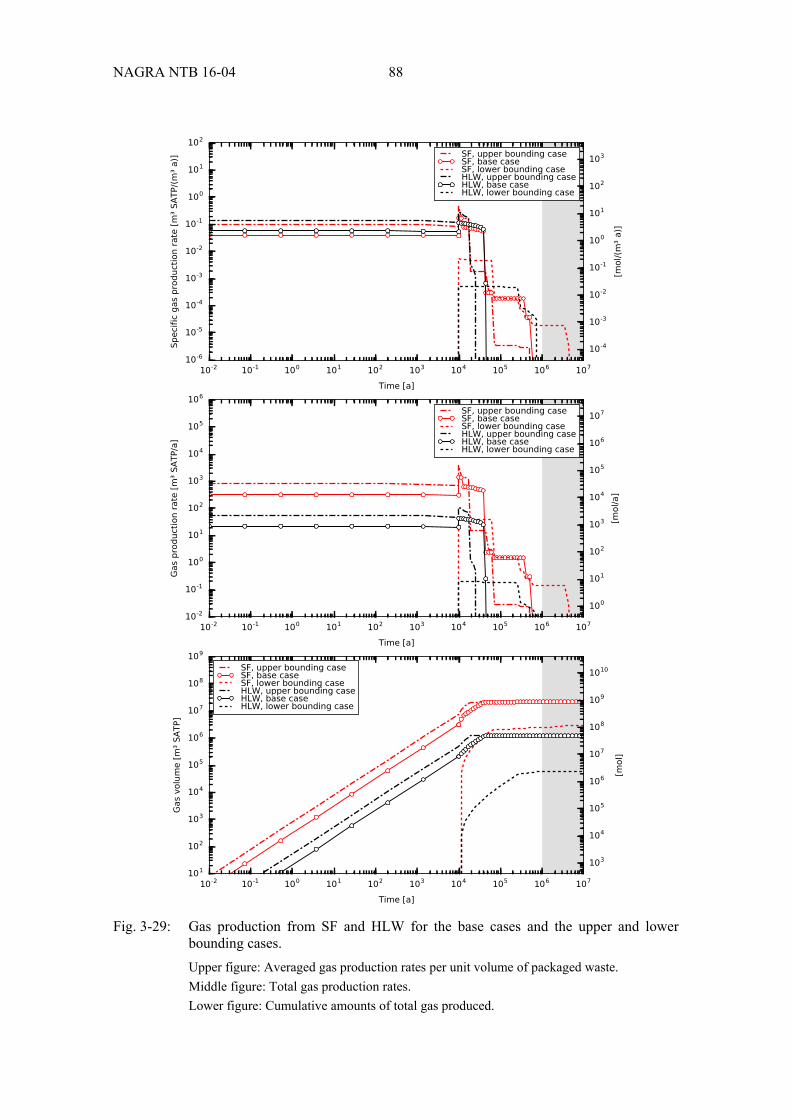
NAGRA NTB 16-04 88
Fig. 3-29: Gas production from SF and HLW for the base cases and the upper and lower
bounding cases. Upper figure: Averaged gas production rates per unit volume of packaged waste. Middle figure: Total gas production rates. Lower figure: Cumulative amounts of total gas produced.

89 NAGRA NTB 16-04
The lower bounding cases for ILW and L/ILW consist of waste allocation to a single ILW emplacement room and L/ILW emplacement room, respectively, with low gas production in the single room considering the entire time frame of safety assessment. Waste allocation to the single room follows the methodology outlined in Section 3.1.1, with the ranking of waste sorts being based on the combination of lower bound corrosion rates, lower bound degradation rates, drums removed, Mosaik-II waste containers replaced with alternative containers that do not significantly produce gas, as well as without pH change due to degradation of organic materials. In the case of L/ILW, the lower bounding case is additionally based on the alternative waste melting scenario (M14AS).38 In the case of ILW, for the sake of simplicity, the potential effect of waste treatment options is not taken into account.
The results for ILW and for L/ILW are presented in Figs. 3-30 and 3-31, respectively. In the upper graph with specific gas production rates, both the results for the single room and the averaged results for all rooms are presented. Again, it can be observed that the gas production rates and gas volumes in the base cases tend to be rather close to those of the upper bounding case (all rooms), reflecting the bias that arises from the definition of the base cases in Sections 2.5 and 3.1.1.
Regarding the results for ILW presented in Fig. 3-30, the following more detailed observations can also be made:
The specific gas production rate in the upper bounding case (single room) is higher than in the lower bounding case (single room) at all times within the period of concern.
The specific gas production rate in the upper bounding case (single room) exceeds the average specific gas production rate in the upper bounding case in the period between around 0.1 years and around 10,000 years; thereafter the rates are similar.
The specific gas production rate in the lower bounding case (single room) is less than the specific gas production rate in the lower bounding case (all rooms) at all calculated times.
The total gas production rate is higher in the upper bounding case than in the lower bounding case, except at times beyond a few hundred thousand years, when the converse is true.
The difference in specific gas production rates between upper bounding case and lower bounding case (all rooms) is up to around two orders of magnitude. For a single room this difference increases to more than around four orders of magnitude.
The total (net) amount of gas produced after a million years in the upper bounding case is 1.2 × 10⁶ m3 (SATP) and around 2.8 × 10⁵ m3 (SATP) in the lower bounding case, which is a difference of around a factor of four.
Regarding the results for L/ILW presented in Fig. 3-31, the following more detailed observations can be made:
The specific gas production rate in the upper bounding case (single room) is higher than in the lower bounding case (single room) at all times within the period of concern.
The specific gas production rate in the upper bounding case (single room) exceeds the specific gas production rate in the upper bounding case (all rooms) after a few years and until the end of the time frame for safety assessment.
38 Pyrolysis is not included in the lower bounding case, since the potential (small) effect (cf. Section 3.1.3) is
masked by the zero lower bound degradation rates and may even lead to an increase in averaged volume-specific gas production rate if fewer emplacement rooms were required.
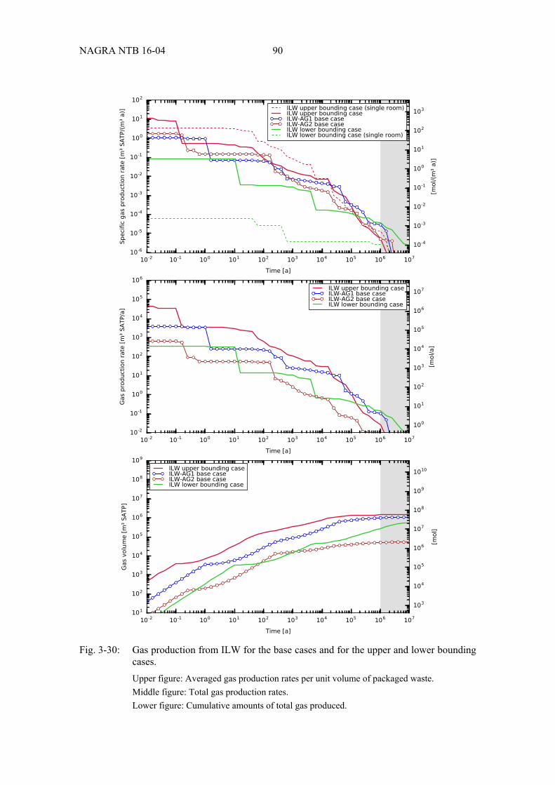
NAGRA NTB 16-04 90
Fig. 3-30: Gas production from ILW for the base cases and for the upper and lower bounding
cases. Upper figure: Averaged gas production rates per unit volume of packaged waste. Middle figure: Total gas production rates. Lower figure: Cumulative amounts of total gas produced.

91 NAGRA NTB 16-04
Fig. 3-31: Gas production from L/ILW for the base cases and for the upper and lower
bounding cases. Upper figure: Averaged gas production rates per unit volume of packaged waste. Middle figure: Total gas production rates. Lower figure: Cumulative amounts of total gas produced.

NAGRA NTB 16-04 92
The specific gas production rate in the lower bounding case (single room) is less than the specific gas production rate in the lower bounding case (all rooms) at all calculated times.
The total gas production rate is higher in the upper bounding case than in the lower bounding case, except at times beyond a few hundred thousand years (and thus beyond the time frame for safety assessment), when the opposite is true.
The total (net) amount of gas produced after one hundred thousand years in the upper bounding case is 3.0 × 10⁷ m3 (SATP) and 9.1 × 10⁵ m3 (SATP) in the lower bounding case, which is a difference of around a factor of thirty.
Table 3-7 summarises the total amounts of gas produced and water consumed by the end of the respective time frames for safety assessment in the base case(s) and in the upper and lower bounding cases in units of m3 (SATP). Table 3-8 provides the equivalent information in units of moles.
In the lower bounding cases for ILW and L/ILW (as well as in all cases for SF and HLW), the only gas species produced is H2 and gross production and net production are equal. This is in contrast to the ILW and L/ILW base cases and upper bounding cases, where some of the gas species, e.g. CO2 from the degradation of organic materials, react at the point of origin with the cement in the ILW and L/ILW near-field, thus resulting in the net production being (slightly) lower than the gross production.
The difference in total amounts of gas produced from SF throughout the period of concern is about a factor of 10 and the corresponding difference for HLW is about a factor of 20. The difference between SF and HLW is a factor of 20 in the upper bounding case and a factor of 40 in the lower bounding case.
The difference in total amounts of gas produced from L/ILW throughout the period of concern is about a factor of 30 and the corresponding difference for ILW is about a factor of 5. The difference between L/ILW and ILW is a factor of 20 in the upper bounding case and a factor of 3 in the lower bounding case.

93 NAGRA NTB 16-04
Tab. 3-7: Total amounts of gas produced [m3 SATP] and water consumed [kg] by the end of the respective time frames for safety assessment in the base case(s) and in the bounding cases. For the L/ILW repository the time frame for safety assessment is 105 a.
For the HLW respository comprising the waste categories SF, HLW and ILW, the time frame for safety assessment is 106 a.
Calcu-lation case
Gas produced [m3 SATP] Water consumed
[kg] H2 CH4 NH3 CO2 H2S Gross Net
SF Upper bounding case
2.2 × 10⁷ 0 0 0 0 2.2 × 10⁷ 2.2 × 10⁷ 1.6 × 10⁷
Base case 2.2 × 10⁷ 0 0 0 0 2.2 × 10⁷ 2.2 × 10⁷ 1.6 × 10⁷ Lower bounding case
2.5 × 10⁶ 0 0 0 0 2.5 × 10⁶ 2.5 × 10⁶ 1.8 × 10⁶
HLW Upper bounding case
1.2 × 10⁶ 0 0 0 0 1.2 × 10⁶ 1.2 × 10⁶ 8.8 × 10⁵
Base case 1.2 × 10⁶ 0 0 0 0 1.2 × 10⁶ 1.2 × 10⁶ 8.8 × 10⁵ Lower bounding case
5.8 × 10⁴ 0 0 0 0 5.8 × 10⁴ 5.8 × 10⁴ 4.2 × 10⁴
ILW Upper bounding case
1.1 × 10⁶ 2.5 × 10⁴ 1.8 × 10³ 1.8 × 10⁴ 6.8 × 10² 1.2 × 10⁶ 1.2 × 10⁶ 8.6 × 10⁵
Base case (AG1) 9.7 × 10⁵ 1.4 × 10⁴ 1.6 × 10³ 1.0 × 10⁴ 6.7 × 10² 9.9 × 10⁵ 9.8 × 10⁵ 7.2 × 10⁵
Base case (AG2) 4.0 × 10⁴ 1.0 × 10⁴ 1.2 × 10² 8.1 × 10³ 8.3 5.8 × 10⁴ 5.0 × 10⁴ 3.5 × 10⁴
Lower bounding case
2.8 × 10⁵ 0 0 0 0 2.8 × 10⁵ 2.8 × 10⁵ 2.1 × 10⁵
L/ILW Upper bounding case
2.8 × 10⁷ 2.1 × 10⁶ 1.1 × 10⁵ 1.4 × 10⁶ 9.3 × 10⁴ 3.2 × 10⁷ 3.0 × 10⁷ 2.2 × 10⁷
Base case (AG1) 2.2 × 10⁷ 8.8 × 10⁵ 8.0 × 10⁴ 6.3 × 10⁵ 6.7 × 10⁴ 2.4 × 10⁷ 2.3 × 10⁷ 1.7 × 10⁷
Base case (AG2) 2.1 × 10⁶ 1.3 × 10⁶ 2.6 × 10⁴ 7.5 × 10⁵ 2.6 × 10⁴ 4.2 × 10⁶ 3.4 × 10⁶ 2.5 × 10⁶
Lower bounding case
9.1 × 10⁵ 0 0 0 0 9.1 × 10⁵ 9.1 × 10⁵ 7.0 × 10⁵

NAGRA NTB 16-04 94
Tab. 3-8: Total amounts of gas produced and water consumed [mol] by the end of the respective time frames for safety assessment in the base case(s) and in the bounding cases. For the L/ILW repository the time frame for safety assessment is 105 a.
For the HLW respository comprising the waste categories SF, HLW and ILW, the time frame for safety assessment is 106 a.
Calcu-lation case
Gas produced [mol] Water consumed
[mol] H2 CH4 NH3 CO2 H2S Gross Net
SF Upper bounding case
8.8 × 10⁸ 0 0 0 0 8.8 × 10⁸ 8.8 × 10⁸ 8.7 × 10⁸
Base case 8.8 × 10⁸ 0 0 0 0 8.8 × 10⁸ 8.8 × 10⁸ 8.7 × 10⁸ Lower bounding case
9.9 × 10⁷ 0 0 0 0 9.9 × 10⁷ 9.9 × 10⁷ 9.9 × 10
HLW Upper bounding case
4.9 × 10⁷ 0 0 0 0 4.9 × 10⁷ 4.9 × 10⁷ 4.9 × 10⁷
Base case 4.9 × 10⁷ 0 0 0 0 4.9 × 10⁷ 4.9 × 10⁷ 4.9 × 10⁷ Lower bounding case
2.4 × 10⁶ 0 0 0 0 2.4 × 10⁶ 2.4 × 10⁶ 2.4 × 10⁶
ILW Upper bounding case
4.6 × 10⁷ 1.0 × 10⁶ 7.1 × 10⁴ 7.3 × 10⁵ 2.7 × 10⁴ 4.7 × 10⁷ 4.7 × 10⁷ 4.8 × 10⁷
Base case (AG1) 3.9 × 10⁷ 5.8 × 10⁵ 6.7 × 10⁴ 4.0 × 10⁵ 2.7 × 10⁴ 4.0 × 10⁷ 4.0 × 10⁷ 4.0 × 10⁷
Base case (AG2) 1.6 × 10⁶ 4.2 × 10⁵ 5.0 × 10³ 3.3 × 10⁵ 3.4 × 10² 2.4 × 10⁶ 2.0 × 10⁶ 1.9 × 10⁶
Lower bounding case
1.1 × 10⁷ 0 0 0 0 1.1 × 10⁷ 1.1 × 10⁷ 1.1 × 10⁷
L/ILW Upper bounding case
1.1 × 10⁹ 8.6 × 10⁷ 4.3 × 10⁶ 5.6 × 10⁷ 3.7 × 10⁶ 1.3 × 10⁹ 1.2 × 10⁹ 1.2 × 10⁹
Base case (AG1) 8.8 × 10⁸ 3.5 × 10⁷ 3.2 × 10⁶ 2.5 × 10⁷ 2.7 × 10⁶ 9.5 × 10⁸ 9.2 × 10⁸ 9.2 × 10⁸
Base case (AG2) 8.4 × 10⁷ 5.1 × 10⁷ 1.0 × 10⁶ 3.0 × 10⁷ 1.0 × 10⁶ 1.7 × 10⁸ 1.4 × 10⁸ 1.4 × 10⁸
Lower bounding case
3.7 × 10⁷ 0 0 0 0 3.7 × 10⁷ 3.7 × 10⁷ 3.9 × 10⁷

95 NAGRA NTB 16-04
3.2 Construction materials
Gas generation from construction materials (including other materials that remain underground after repository closure) is calculated based on the input data described in Section 2.3.2 and according to the list of assessment cases in Table 2-4.
The analysis is carried out separately for the different room profiles of the HLW repository and the L/ILW repository (cf. Table 2-1). Details on the total amounts (including uncertainties) and properties of gas-generating construction materials are listed in Table B-2.
As outlined in Section 2.1.1, the modelling period extends beyond the respective time frames for safety assessment, which are 105 years for the L/ILW repository and 106 years for the HLW repository. In the presentation of the results, this part of the modelling period is indicated with one or two shaded regions.
3.2.1 Base case
The base case is the starting-point for the systematic and deterministic exploration of relevant uncertainties and options. It draws on the reference conceptual and modelling assumptions presented in Sections 2.1 and 2.2, which tend to overestimate gas production in terms of total amounts, in terms of rates at early times, or both.
According to the general assumptions in Section 2.1.1, the calculated gas generation rates and the calculated cumulative amounts of gas produced are presented in volumetric quantities. Since all gas-generating construction materials are assumed to be made of carbon steel, hydrogen is the only gas species produced. Thus, in the case of construction materials (unlike waste and disposal containers), there is no need to distinguish between gross and net gas production.
In the calculations presented in this section, rates and cumulative amounts of water consumed are determined by the reaction for hydrogen gas generation from carbon steel. Neither the effects of reactions involving hydrogen subsequent to its production, which may also consume or produce water, nor the pure dissolution of hydrogen in the aqueous phase are included in the results.
Gas production rates, water consumption rates and total amounts of gas produced / water consumed are given per unit length of the individual profiles. Total rates and total amounts are not reported because this study does not refer to specific repository layouts.
Water consumption is discussed only for the base case, with the remainder of Section 3.2 dealing with gas production only. However, it should be kept in mind that, for each length-specific gas generation rate, an associated length-specific water consumption rate is also calculated for subsequent use in gas / water transport studies and gas consumption studies.
Similarly, gas production for profiles that are not part of emplacement rooms are discussed only for the base case and not in the remainder of Section 3.2. This is intended to enhance the readability of the figures, given the numerous profiles that are considered. Note that gas pro-duction for profiles in the emplacement rooms covers the range of all profiles, as shown further below. Note also that, despite not being reported, the respective alternative cases are calculated for all profiles for subsequent use in gas / water transport studies and gas consumption studies.

NAGRA NTB 16-04 96
Gas production
Fig. 3-32 shows length-specific gas production rates and length-specific cumulative amounts of gas produced for the different profiles in the HLW repository and in the L/ILW repository.
Fig. 3-32: Gas production for different profiles in the base case.
Upper figure: Length-specific gas production rates. Lower figure: Length-specific cumulative amounts of gas produced.

97 NAGRA NTB 16-04
The following observations can be made:
For all profiles, the gas production rates remain constant for about 2,000 years. During this period, the rates are between 0.01 m3 (SATP) a-1 per unit tunnel length for profile F and 0.2 m3 (SATP) a-1 per tunnel length for profile K09. In the period between 2,000 years and 20,000 years, the gas production rates continuously decrease and finally reach values below 5 × 10⁻³ m3 (SATP) a-1 per tunnel length for all tunnel types.
For several of the profiles, an inflection in the gas production rates is visible at around 10,000 years. This is explained by the fact that, with the exception of the profile ZS, initial gas generation is dominated by steel anchors and steel fibres, which are fully corroded after around 10,000 years. Thereafter, gas generation is dominated by reinforcing steel meshes and other reinforcement. For profile ZS, only steel arches contribute to gas generation (see Appendix B.2).
The length-specific cumulative amounts of total gas produced after one million years range from 100 m3 (SATP) per tunnel length for profile F to about 1,000 m3 (SATP) per tunnel length for profile K09.
The fact that both gas production rates at early times and cumulative amounts of gas produced are framed by the values obtained for the profiles F and K09 is not surprising, since these profiles show the smallest and the largest diameter, respectively. In the following sections, only gas production for profiles in the emplacement rooms are discussed. This concerns the profiles F (SF/HLW emplacement tunnels), ZS (interjacent sealing sections of SF/HLW emplacement tunnels), K04 (ILW emplacement caverns) and K09 (L/ILW emplacement caverns).
Water consumption
Fig. 3-33 shows length-specific water consumption rates and cumulative amounts of water consumed for the different profiles in the HLW repository and in the L/ILW repository.
The following observations can be made:
For all profiles, the water consumption rates remain constant for about 2,000 years. During this period the rates are between 7 × 10⁻³ kg a-1 per unit tunnel length for profile F and 0.02 kg a-1 per tunnel length for profile K09. In the period between 2,000 years and 20,000 years, the water consumption rates continuously decrease and finally reach values below 3 × 10⁻³ kg a-1 per tunnel length for all tunnel types.
The length-specific cumulative amounts of total water consumed after one million years range from 60 kg per tunnel length for profile F to about 1,000 kg per tunnel length for profile K09.

NAGRA NTB 16-04 98
Fig. 3-33: Water consumption for different profiles in the base case.
Upper figure: Length-specific water consumption rates. Lower figure: Length-specific cumulative amounts of water consumed.

99 NAGRA NTB 16-04
As described in Section 3.1.1, the water consumption by a given corrosion reaction can be derived directly from the corresponding amounts of gas generated using the average water consumption factor given by Equation (24). Since all construction materials are assumed to be made of carbon steel, only one corrosion reaction needs to be considered. The average water consumption factor ̅
/ for carbon steel and other ferrous materials is therefore
1 molH2O/molgas throughout the entire time frame for safety assessment for each repository. Thus, the length-specific water consumption rate can be calculated based on the
length-specific gas production rate by applying the following equation:
⋅ (25)
with the molar gas volume ν = 0.02479 m³ (SATP)/molgas and the molar mass of water = 0.018 kg/molH2O .
Correspondingly, the total mass of water consumed per tunnel length is:
⋅ (26)
Predominant construction components in emplacement rooms
Figs. 3-34 to 3-36 show gas production in SF/HLW emplacement tunnels (profiles F / ZS), ILW emplacement caverns (profile K04) and L/ILW emplacement caverns (profile K09), including the contributions of individual construction components.
The following observations can be made:
In the SF/HLW emplacement tunnels (Fig. 3-34), the highest length-specific gas production rates are from steel arches at the positions of interjacent sealing sections (profile ZS). However, the contribution of the steel arches in profile ZS to overall gas production in the SF/HLW emplacement tunnels is small, since these profiles account for only about 10 % of the entire tunnel length. The length-specific gas production rate of steel anchors at emplacement sections (profile F) is about half the value calculated for the steel arches. Recall that anchor plates are assumed to be removed prior to backfilling of the emplacement tunnels. The length-specific gas production rate of reinforcement meshes (profile F) is negligible, since these are in a cementitious environment with high pH values that substantially reduce the corrosion rate.
In the ILW and L/ILW emplacement rooms (Figs. 3-35 and 3-36), the largest contributions to length-specific gas production rate are also from steel anchors, followed by steel fibres, which provide a contribution about one-third that of steel anchors. The contributions of reinforcement meshes and other reinforcement material in construction concrete are negligible.
The steel anchors also contribute most to the total amount of gas produced at the end of the time frames for safety assessment. The contributions of steel fibres and reinforcement meshes are of minor importance, and the contribution of other reinforcement structures is negligible.

NAGRA NTB 16-04 100
Fig. 3-34: Gas production in SF / HLW emplacement tunnels (profiles F / ZS) in the base
case with details on individual construction components. Upper figure: Length-specific gas production rates for each profile. Lower figure: Length-specific cumulative amounts of gas produced for each profile.

101 NAGRA NTB 16-04
Fig. 3-35: Gas production in ILW emplacement caverns (profile K04) in the base case with
details on individual construction components. Upper figure: Length-specific gas production rates. Lower figure: Length-specific cumulative amounts of gas produced.

NAGRA NTB 16-04 102
Fig. 3-36: Gas production in L/ILW emplacement caverns (profile K09) in the base case with
details on individual construction components. Upper figure: Length-specific gas production rates. Lower figure: Length-specific cumulative amounts of gas produced.

103 NAGRA NTB 16-04
3.2.2 Uncertainties
This section explores the impact of relevant uncertainties starting from the base case. According to Table 2-4, the key uncertainties for construction materials are the corrosion rates and the amounts of construction materials present. In this section, only the results for the profiles in the emplacement rooms are reported.
Corrosion rates
Fig. 3-37 shows length-specific gas production rates and length-specific cumulative amounts of gas produced in the individual emplacement room profiles for the base cases along with results for alternative cases with upper and lower bound corrosion rates for carbon steel.
The following observations can be made:
For all profiles, the upper length-specific gas production rate over the first 1´000 years is about a factor of 2.5 higher than the rate in the base case, whereas the lower rate at early times is reduced by a factor of about 20. These ratios are similar to those of the upper and lower corrosion rates for steel arches and steel anchors in the clay environment (cf. Table A-2).
In the case of profiles F, K04 and K09, the total amounts of gas produced at the end of the respective time frames for safety assessment using the reference corrosion rates are the same as those using the upper bound values; for the lower bound values the total amounts are about a factor of 2 lower, but converge 1-2 million years later. In the case of profile ZS, the total amounts of gas produced are independent of the corrosion rates applied.
Amounts of construction materials
Reference values for the amounts of construction materials are reported in Table B-2. This table also provides information on the associated uncertainties. Upper bound values are provided only for the masses of steel fibres in the different profiles. Lower bound values are available for the masses of steel anchors, steel fibres and reinforcing steel meshes. For all remaining construction components, the associated uncertainty is considered negligible.
Fig. 3-38 shows length-specific gas production rates and length-specific cumulative amounts of gas produced in the individual profiles for the emplacement rooms in the base cases along with alternative cases with upper and lower bound values for the amounts of construction materials.
The following observations can be made:
Since the profile F does not contain any steel fibres, the gas production rates for high amounts of construction materials and the reference gas production rates are identical.
Gas production rates at early times for profiles F, K04 and K09 and with high or low amounts of construction materials differ by less than a factor of two from the respective gas production rates in the base case.

NAGRA NTB 16-04 104
Fig. 3-37: Gas production in individual emplacement room profiles for the base cases and for
alternative cases with upper bound and lower bound corrosion rates. Upper figure: Length-specific gas production rates. Lower figure: Length-specific cumulative amounts of gas produced.

105 NAGRA NTB 16-04
Fig. 3-38: Gas production in individual emplacement room profiles for the base cases and for
alternative cases with upper bound and lower bound values for the amounts of construction materials. Upper figure: Length-specific gas production rates. Lower figure: Length-specific cumulative amounts of gas produced.

NAGRA NTB 16-04 106
3.2.3 Options
This section explores the potential impact of relevant options that exist for the construction materials (including other materials that remain underground after repository closure) starting from the base case. According to Table 2-4, these options concern the support concept at the positions of interjacent sealing sections in SF/HLW emplacement tunnels, and the technology applied to emplace SF and HLW disposal canisters and subsequently backfill the emplacement tunnels.
Concept for interjacent sealing sections in SF and HLW emplacement tunnels
In the base case, it is assumed that tunnel support at the positions of interjacent sealing sections in SF/HLW emplacement tunnels is provided by a series of steel arches.
Fig. 3-39 shows length-specific gas production rates and length-specific cumulative amounts of gas produced in the profile ZS (interjacent sealing section) for the base case and for an alternative case with tunnel support provided by a liner, as in the non-seal sections.
The results show that length-specific gas production rates when using a liner are at most a factor of two below the gas production rates when using steel arches. The same observation is made with regard to the cumulative amounts of gas produced after one million years. Thus, using a liner would lower gas production in the interjacent sealing sections to some extent. However, the contribution of tunnel support in the interjacent sealing sections to overall gas production in SF/HLW emplacement tunnels is in any case small, since these sections account for only about 10 % of the entire tunnel length.
Emplacement and backfilling technology for SF and HLW
In the base case, it is assumed that emplacement of SF and HLW disposal canisters, as well as backfilling of SF/HLW emplacement tunnels, does not rely on rail-based technology.
Fig. 3-40 shows length-specific gas production rates and length-specific cumulative amounts of gas produced in the profiles F (emplacement section) and ZS (interjacent sealing section) for the base case and for an alternative case with rail-based emplacement and backfilling technology according to Nagra's Full-scale Emplacement Experiment (FE) at the Mont Terri underground research laboratory (Jenni & Köhler 2015).
The following observations can be made:
Using rails results in a gas production rate at early times that is about a factor of two higher in the case of profile ZS and a factor of 2.5 higher in the case of profile F. The effect is less pronounced in the former case, since the steel arches in profile ZS already provide a slightly higher contribution to gas production than the steel anchors in profile F.
With respect to the cumulative amounts after one million years, the effect for profile F is slightly less pronounced than for ZS; the use of rails makes a difference well below a factor of two for both profiles.

107 NAGRA NTB 16-04
Fig. 3-39: Gas production in profile ZS (interjacent sealing section) for the base case and for
an alternative case with tunnel support provided by liner. Upper figure: Length-specific gas production rates. Lower figure: Length-specific cumulative amounts of gas produced.

NAGRA NTB 16-04 108
Fig. 3-40: Gas production in profiles F (emplacement section) and ZS (interjacent sealing
section) for the base cases and for alternative cases with rail-based emplacement and backfilling technology. Upper figure: Length-specific gas production rates. Lower figure: Length-specific cumulative amounts of gas produced.

109 NAGRA NTB 16-04
3.2.4 Bounding cases
This section deals with the analysis of the bounding cases for gas generation from construction materials (including other materials that remain underground after repository closure). The construction of the bounding cases is based on the summary of key uncertainties in Section 2.5.1 and on the findings of the exploration of model / parameter uncertainties and options in Sections 3.2.2 and 3.2.3. In this section, only the results for the profiles in the emplacement rooms are reported.
The upper bounding case for all profiles except profiles F and ZS (sections of the SF / HLW emplacement tunnels) consists of a combination of upper bound corrosion rates and upper bound values for the amounts of construction materials. The upper bounding case for the pro-files F and ZS consists of a combination of rail-based emplacement and backfilling technology with upper bound corrosion rates and with upper bound values for the amounts of construction materials.
The lower bounding case for all profiles except profile ZS (section in the SF / HLW emplace-ment tunnels with interjacent sealing sections) consists of a combination of lower bound corrosion rates with lower bound values for the amounts of construction materials. The lower bounding case for the profile ZS consists of a combination of tunnel lining at the positions of interjacent sealing sections with lower bound corrosion rates and with lower bound values for the amounts of construction materials.
The results for the individual profiles are presented in Fig. 3-41. As in the analyses of the waste and disposal containers, it can be observed that the gas production rates and gas volumes in the base case tend to be rather close to those of the upper bounding case, reflecting the bias that arises from the definition of the base case in Sections 2.5 and 3.2.1.
The following more detailed observations can also be made:
For profile F (emplacement section of the SF / HLW emplacement tunnels), the gas produc-tion rate in the upper bounding case is considerably higher at early times than in the base case. The difference is about a factor of 6 and the maximum value is roughly 6 × 10⁻² m3 (SATP) a-1 per unit tunnel length. The maximum value in the lower bounding case, however, is much lower at 3 × 10⁻⁴ m3 (SATP) a-1 per unit tunnel length, which is a factor of about 30 below the base case. The total variation at early times is thus a factor of about 180. Total amounts of gas produced in the upper bounding case after one million years are only about a factor of 1.5 higher than in the base case. The respective value for the lower bounding case is about a factor of 3 below the value in the base case.
For profile ZS (section of the SF / HLW emplacement tunnel with interjacent sealing elements), the gas production rate in the upper bounding case is considerably higher at early times than in the base case. The difference is about factor of 4 and the maximum value is roughly 8 × 10⁻² m3 (SATP) a-1 per unit tunnel length. The maximum value in the lower bounding case, however, is much lower at 3 × 10⁻⁴ m3 (SATP) a-1 per unit tunnel length, which is about a factor of 7 below the base case. The total variation at early times is thus a factor of about 28. As for profile F, total amounts of gas in the upper bounding case after one million years are only about a factor of 1.5 higher than in the base case. The respective value for the lower bounding case is a factor of about 5 below the value in the base case.

NAGRA NTB 16-04 110
Fig. 3-41: Gas production in individual emplacement room profiles for the base cases and for
the upper and lower bounding cases. Upper figure: Length-specific gas production rates. Lower figure: Length-specific cumulative amounts of gas produced.

111 NAGRA NTB 16-04
For profile K04 (emplacement room for ILW), the gas production rate in the upper bounding case is markedly higher at early times than in the base case. The difference is about a factor of 2.5 and the maximum value is roughly 3 × 10⁻¹ m3 (SATP) a-1 per unit tunnel length. The maximum value in the lower bounding case, however, is much lower at 4 × 10⁻³ m3 (SATP) a-1 per unit tunnel length, which is a factor of about 40 below the base case value. The total variation at early times is thus a factor of about 100. Total amounts of gas in the upper bounding case after one million years are only slightly higher than in the base case. The respective value for the lower bounding case is a factor of about 1.5 below the value in the base case.
For profile K09 (emplacement room for L/ILW), the observed behaviour is rather similar to that of profile K04. The gas production rate in the upper bounding case is markedly higher at early times than in the base case. The difference is about a factor of 2.5 and the maximum value is roughly 4 × 10⁻¹ m3 (SATP) a-1 per unit tunnel length. The maximum value in the lower bounding case, however, is much lower at 5 × 10⁻³ m3 (SATP) a-1 per unit tunnel length, which is a factor of about 40 below the base case value. The total variation at early times is thus a factor of about 100. Total amounts of gas in the upper bounding case after one 105 years are only slightly higher than in the base case. The respective value for the lower bounding case is a factor of about 2.5 below the value in the base case.
3.3 Comparison for emplacement rooms
In this section, the gas production rates and cumulative amounts of gas produced from waste and disposal containers (base case and bounding cases) are compared with those from the construction materials in the respective emplacement rooms (base case and bounding cases). To this end, volume-specific gas production rates and cumulative amounts of gas produced from waste and disposal containers are converted to length-specific variables by using the conversion factors (average emplacement densities of packaged waste) given in Section 2.3.1. In addition, the total amounts of gas produced in all emplacement rooms for each waste category are shown for the respective base cases in Table 3-9. The total amounts for the interjacent sealing sections in SF/HLW emplacement tunnels are calculated based on the geometric assumptions given in Section 2.3.2.
Note that gas production from waste and disposal containers is not independent from gas production from construction materials. Rather, the two are linked via the environmental conditions (including water supply) in the individual emplacement rooms. The occurrence of a rather high gas production from waste and disposal containers together with a rather low gas production from construction materials is therefore improbable.
The results for SF emplacement tunnels are presented in Fig. 3-42 and Table 3-9. The following observations are made:
Regarding both length-specific gas production rates and gas volumes, there is a high degree of overlap between the range of gas generation for waste and disposal canisters on the one hand and the range of gas generation for construction materials on the other hand. Thus, it is not apparent a priori which group of gas sources plays the dominant role.

NAGRA NTB 16-04 112
Tab. 3-9: Comparison of total amounts of gas produced [m3 SATP] and water consumed [kg] from waste and disposal containers vs. construction materials by the end of the respective time frames for safety assessment in the base case. For the L/ILW repository the time frame for safety assessment is 105 a.
For the HLW respository comprising of the waste categories SF, HLW and ILW, the time frame for safety assessment is 106 a.
Gas source
Gas produced [m3 SATP] Water
H2 CH4 NH3 CO2 H2S Gross Net [kg]
SF emplacement tunnels
SF 2.2 × 10⁷ 0 0 0 0 2.2 × 10⁷ 2.2 × 10⁷ 1.6 × 10⁷
F 1.5 × 10⁶ 0 0 0 0 1.5 × 10⁶ 1.5 × 10⁶ 1.1 × 10⁶
ZS 3.1 × 10⁵ 0 0 0 0 3.1 × 10⁵ 3.1 × 10⁵ 2.2 × 10⁵
HLW emplacement tunnels
HLW 1.2 × 10⁶ 0 0 0 0 1.2 × 10⁶ 1.2 × 10⁶ 8.8 × 10⁵
F 1.8 × 10⁵ 0 0 0 0 1.8 × 10⁵ 1.8 × 10⁵ 1.3 × 10⁵
ZS 4.6 × 10⁴ 0 0 0 0 4.6 × 10⁴ 4.6 × 10⁴ 3.3 × 10⁴
ILW-AG1 emplacement rooms
ILW- AG1 9.7 × 10⁵ 1.4 × 10⁴ 1.6 × 10³ 1.0 × 10⁴ 6.7 × 10² 9.9 × 10⁵ 9.8 × 10⁵ 7.2 × 10⁵
K04 1.4 × 10⁵ 0 0 0 0 1.4 × 10⁵ 1.4 × 10⁵ 9.9 × 10⁴
ILW-AG2 emplacement rooms
ILW- AG2 4.0 × 10⁴ 1.0 × 10⁴ 1.2 × 10² 8.1 × 10³ 8.3 5.8 × 10⁴ 5.0 × 10⁴ 3.5 × 10⁴
K04 1.4 × 10⁴ 0 0 0 0 1.4 × 10⁴ 1.4 × 10⁴ 1.0 × 10⁴
L/ILW-AG1 emplacement rooms
L/ILW- AG1 2.2 × 10⁷ 8.8 × 10⁵ 8.0 × 10⁴ 6.3 × 10⁵ 6.7 × 10⁴ 2.4 × 10⁷ 2.3 × 10⁷ 1.7 × 10⁷
K09 1.5 × 10⁶ 0 0 0 0 1.5 × 10⁶ 1.5 × 10⁶ 1.1 × 10⁶
L/ILW-AG2 emplacement rooms
L/ILW- AG1 2.1 × 10⁶ 1.3 × 10⁶ 2.6 × 10⁴ 7.5 × 10⁵ 2.6 × 10⁴ 4.2 × 10⁶ 3.4 × 10⁶ 2.5 × 10⁶
K09 2.9 × 10⁵ 0 0 0 0 2.9 × 10⁵ 2.9 × 10⁵ 2.1 × 10
In the base case, the length-specific gas production rate from SF and disposal canisters
exceeds those from the construction materials in interjacent sealing sections (profile ZS) and in disposal sections (profile F) at all times, with the exception of the period from around 50,000 years to a little over 100,000 years, when the length-specific gas production from construction materials in disposal sections (profile F) exceeds that from SF and disposal canisters. For the first few hundred years, however, the gas production rate from SF and disposal canisters is only slightly higher than that from the construction materials in interjacent sealing sections (profile ZS).

113 NAGRA NTB 16-04
In the upper bounding case for gas production from construction materials, length-specific gas production rates for disposal sections (profile F) are very similar to the length-specific gas production rates from SF and the disposal canisters (upper bounding case) up to around one thousand years. Length-specific gas production rates for construction materials in the interjacent sealing sections (profile ZS) in the upper bounding case are slightly higher than the length-specific gas production rates from SF and disposal canisters (upper bounding case), again up to around one thousand years, following which production rates from the SF and disposal canisters are maintained, while production rates from the construction materials in the interjacent sealing sections (profile F) decline.
In the lower bounding case, which is based on an alternative canister material that does not significantly produce gas, gas production from the canister internals starts when gas production from construction materials is already declining.
In the long term, after a few thousand years the total volume of gas produced by SF and disposal canisters dominates over that produced by the construction materials in the disposal sections (profile F) by about one order of magnitude, unless the lower bounding case for SF and disposal canisters is assumed, in which case the gas volumes produced in the long term from SF and disposal canisters are similar to those of the base case or upper bounding case for the construction materials in the disposal sections (profile F). The total volume of gas produced in interjacent sealing sections (profile ZS) is small (Table 3-9).
The results for HLW emplacement tunnels are presented in Fig. 3-43 and Table 3-9. The following observations are made:
Regarding both length-specific gas production rates and gas volumes, as in the case of SF, there is a high degree of overlap between the range of gas generation for waste and disposal canisters on the one hand and the range of gas generation for construction materials on the other hand. Thus, it is not apparent a priori which group of gas sources plays the dominant role.
In the base case, the length-specific gas production rate from HLW and disposal canisters for the first few hundred years is slightly higher than that from the construction materials in disposal sections (profile F), but less than that from construction materials in the interjacent sealing sections (profile ZS). Thereafter, gas production from the construction materials in disposal sections (profile F) falls, while that from HLW and disposal canisters, as well as that from construction materials in interjacent sealing sections (profile ZS) is maintained. After some tens of thousands of years, length-specific gas production from HLW and disposal canisters falls rapidly to values less than the remaining production rates from construction materials in disposal sections (profile F).
In the upper bounding case, the length-specific gas production rate from HLW and disposal canisters is less than the upper bound values from construction materials in disposal sections (profile F) and in interjacent sealing sections (profile ZS) for the first two to three thousand years. Thereafter, length-specific gas production rates are dominated by HLW and disposal canisters until around 40,000 years, when the rate from HLW and disposal canisters drops below that from the construction materials in disposal sections (profile F).
In the lower bounding case, which is based on an alternative canister material that does not significantly produce gas, gas production from the canister internals starts when gas production from construction materials is already declining.

NAGRA NTB 16-04 114
Fig. 3-42: Comparison of gas production from waste and disposal containers vs. construction
materials in an SF emplacement tunnel. Upper figure: Length-specific gas production rates. Lower figure: Length-specific cumulative amounts of gas produced.

115 NAGRA NTB 16-04
Fig. 3-43: Comparison of gas production from waste and disposal containers vs. construction
materials in an HLW emplacement tunnel. Upper figure: Length-specific gas production rates. Lower figure: Length-specific cumulative amounts of gas produced.

NAGRA NTB 16-04 116
In the long term, after a few thousand years the total volume of gas produced by HLW and disposal canisters dominates over that produced by the construction materials (profile F) by about a factor of seven, unless the lower bounding case for HLW and disposal canisters is assumed, in which case the gas volumes produced in the long term from HLW and disposal canisters are generally less than those for the construction materials (profile F). The total volume of gas produced in interjacent sealing sections (profile ZS) is small (Table 3-9).
The results for ILW emplacement rooms are presented in Fig. 3-44 and Table 3-9. Note that in Fig. 3-44 both the results for the single room and the averaged results for all rooms are presented. The following observations are made:
Regarding both length-specific gas production rates and gas volumes, there is some degree of overlap between the range of gas generation for waste and disposal containers on the one hand and the range of gas generation for construction materials on the other hand for certain time periods. Thus, it is not apparent a priori which group of gas sources plays the dominant role during these periods. Nevertheless, the conclusion can be drawn that even during these periods gas production from waste and disposal containers plays – on average – a more dominant role than gas production from construction materials, since both types of gas sources are linked via the environmental conditions in the emplacement rooms (cf. discussion on the emplacement density of gas-generating materials in Section 3.1.1).
In the base case, gas production rates after a few hundred years are generally rather similar for ILW-AG1 and ILW-AG-2. They are initially higher than the rates from construction materials up to around 1,000 years, but thereafter are quite similar to the base case and upper bound gas production rates from construction materials.
In the lower bounding case for profile K04, the gas production rates from construction materials are less than those from the waste and disposal containers in the ILW-AG1 and ILW-AG2 base cases for all calculated times.
Looking at single emplacement rooms rather than the entire ILW waste category (all rooms), the resulting range of uncertainty in gas production is very high. In particular, the gas production rates from construction materials in all cases exceed those from a single room filled with the least intensely gas-producing waste types (ILW, lower bounding case (single room)) for at least 200,000 years, whereas they are less than those from a single room filled with the most intensely gas-producing waste types (ILW, upper bounding case (single room)) at all times. Thus, for a single room far more than for the average over all ILW emplacement rooms, the uncertainty regarding gas generation (and resulting effects such as gas saturation and mobility of dissolved radionuclides) is considerable.
The gas volume produced after one million years from construction materials is about a factor of around four to seven less than that produced from the waste and disposal containers in all cases, except for the case of a single room filled with the least intensely gas-producing waste types (ILW, lower bounding case (single room)).

117 NAGRA NTB 16-04
Fig. 3-44: Comparison of gas production from waste and disposal containers vs. construction
materials in an ILW emplacement room. Upper figure: Length-specific gas production rates. Lower figure: Length-specific cumulative amounts of gas produced.

NAGRA NTB 16-04 118
The results for L/ILW emplacement rooms are presented in Fig. 3-45 and Table 3-9. Note that in Fig. 3-45 both the results for the single room and the averaged results for all rooms are presented. Similar observations can be made as for ILW, although gas production from construction materials tends to be lower relative to that from the waste and disposal containers. More specifically:
In all cases for profile K09, the gas production rates from construction materials are less than those from the waste and containers in the L/ILW-AG1 and L/ILW-AG2 base cases at all calculated times.
In all cases the gas production rates from construction materials are equal to or exceed those from a single room filled with the least intensely gas-producing waste types (L/ILW, lower bounding case (single room)) for more than a hundred thousand years.
The gas volume produced after one hundred thousand years from construction materials is about one order of magnitude less than that produced from the waste and disposal containers in all cases, except for the case of a single room filled with the least intensely gas-producing waste types (ILW, lower bounding case (single room)) and also for the lower bounding case (all rooms).

119 NAGRA NTB 16-04
Fig. 3-45: Comparison of gas production from waste and disposal containers vs. construction
materials in an L/ILW emplacement room. Upper figure: Length-specific gas production rates. Lower figure: Length-specific cumulative amounts of gas produced.


121 NAGRA NTB 16-04
4 Conclusions In deep geological repositories for radioactive waste, significant quantities of gases will be generated in the long term as a result of various processes, most notably the anaerobic corrosion of metals and the degradation of organic materials. Therefore, the impact of gas production on post-closure safety of the repositories needs to be assessed.
In the present report, conceptual and mathematical models for gas generation and water consumption have been developed, based on current scientific knowledge and current preliminary repository designs. The models have been implemented in spreadsheet-based computer tools and applied to provide quantitative estimates of gas generation rates and associated water consumption rates for the post-closure phase of deep geological repositories in Opalinus Clay. Quality assurance of the gas-generation tools has followed Nagra's quality assurance guidelines for safety assessment modelling. It is pointed out that the validity of the models and the results is constrained to the information and premises used in the development of the models.
A systematic and deterministic analysis has been made of the key uncertainties and principal programme and design options available with respect to gas generation and its modelling. The modelling approach adopted does not explicitly consider the coupling with other related processes, namely the transport of gas and water as well as the possible consumption of gas. As a result, many uncertainties have been handled using simplified and stylised model assumptions, thus resulting in base cases that tend to overestimate early gas production rates. The base cases should therefore not be regarded as a description of the most likely or of the expected evolution. On the other hand, care has been taken to ensure that the calculated ranges of gas generation rates and associated water consumption rates cover the full range of possible future evolutions, including the effects of relatively long time periods with unsaturated conditions in the backfilled underground structures. To this end, upper and lower bounding cases have been defined that incorporate combinations of model assumptions, parameter values and programme / design options that each tend, individually, to lead to higher or lower gas production rates than those of the base cases. Within the calculated ranges, the results fall below or exceed the outcomes real-istically to be expected to some extent due to the use of simplified / stylised model assumptions, which needs to be recognised in related modelling and assessment activities.
The following main sources of gas in a deep geological repository have been considered separately in the modelling:
the emplaced waste including the disposal containers, and
the construction materials (including other materials that remain underground after repository closure) within different profiles.
In the disposal rooms, there is generally a high degree of overlap in the ranges for the calculated gas production rates for waste and disposal canisters on the one hand and for construction materials on the other hand. The exceptions are ILW and L/ILW, where gas production rates and total volumes from construction materials tend to be significantly less than those from the waste and disposal containers. For all waste types and profiles, the base case gas production rates and gas volumes tend to be rather close to, or at least of the same order as, those of the upper bounding cases, reflecting the bias that arises from the definition of the base cases.

NAGRA NTB 16-04 122
In the SF and HLW base cases, gas production occurs predominantly during the first 40,000 years after closure, while corrosion of the reference carbon steel disposal canister is ongoing. It is dominated by hydrogen production from the corrosion of:
the outer surfaces of the disposal canisters, and once the canisters have been breached by
the inner canister surfaces, as well as corrosion of the baskets for the SF assemblies, the SF assemblies themselves (steel and Zircaloy) and the surfaces of the HLW steel flasks, and
to a lesser extent, steel anchors in the emplacement sections.
The contribution of steel arches in the interjacent sealing sections to overall gas production in SF/HLW emplacement tunnels is small, since these sections do account for only about 10 % of the entire tunnel length.
The gas volume produced from SF during the million-year time period for safety assessment is around an order of magnitude higher than that produced by the corrosion of construction materials. For HLW, it is a factor of about seven higher than that from construction materials. Uncertainties in the corrosion rates of metals can significantly affect gas generation rates, but do not affect the total volumes of gas produced during the million-year time period for safety assessment.
The gas generation rates and volumes of gas produced by the corrosion of construction materials are increased, again by a factor of around two, if rail-based technology is used for SF/HLW disposal canister emplacement and tunnel backfilling. Regardless of whether rails are used or not, corrosion of the reference carbon steel canister and its internals remains the dominant gas production process in terms of total volumes.
If the SF and HLW disposal canisters are assumed to be fabricated of a material that has negligible gas production, rather than carbon steel, gas production associated with SF and HLW commences only once the canisters are breached, which itself occurs when gas production from construction materials is already declining. Sources of gas are then limited to the baskets for the SF assemblies, the SF assemblies themselves (steel and Zircaloy) and the outer surfaces of the HLW steel flasks. The gas volumes produced by these sources during the million-year time period for safety assessment are about an order of magnitude less than in the respective base cases, and are hence rather similar to those produced by the construction materials.
In the ILW base cases, the total gas volume produced from the waste during the million-year time period for safety assessment is a factor of around four to seven higher than that from the construction materials. Gas production from the waste is generally dominated by hydrogen production from the corrosion of cast iron Mosaik-II waste containers for PWR internals, along with corrosion of aluminium in operational waste from the surface facility of the HLW repository. Uncertainties in the corrosion rates of metals can significantly affect gas generation rates, but have a minor influence on the total volumes of gas produced during the million-year time period for safety assessment. The potential impact of local heterogeneities in pH associated with the degradation of organic materials affecting corrosion rates is small. For waste group ILW-AG2, additional significant contributions to gross gas production come from carbon dioxide and methane from the degradation of various organic substances. However, the total amounts of gas produced for waste group ILW-AG2 are substantially lower than those for waste group ILW-AG1 and almost all intensely gas-producing waste types belong to waste group AG1. Furthermore, carbon dioxide is expected to react entirely with cement immediately upon production and so does not contribute to net gas production. Thus, overall, the degradation of organic materials does not significantly affect gas production in the case of ILW over the million-year time period for safety assessment.

123 NAGRA NTB 16-04
In the L/ILW base cases, the total gas volume produced from the waste during the hundred-thousand-year time period for safety assessment is around an order of magnitude higher than that from the construction materials. Gas production is generally dominated by hydrogen production from the corrosion of carbon steel in decommissioning waste from the PSI-West research facilities and from the Beznau and Leibstadt reactors. However, recent analyses have led to an update of the inventory of decommissioning waste from the PSI-West research facility and an analysis of the updated inventory in the present report shows that the respective waste types are less predominant than in the original inventory. Uncertainties in the corrosion rates of metals can significantly affect gas generation rates and also affect (more significantly than in the case of ILW) the total volumes of gas produced during the hundred-thousand-year time period for safety assessment. The potential impact of local heterogeneities in pH associated with the degradation of organic materials affecting corrosion rates is small. Intensely gas-producing waste types are present in both waste groups L/ILW-AG1 and L/ILW-AG2 and significant contributions to gross gas production in L/ILW-AG2 come from carbon dioxide and methane from the degradation of various organic substances. However, as in the case of ILW, the total amounts of L/ILW-AG2 are substantially lower than those of L/ILW-AG1 and carbon dioxide is expected to react entirely with cement immediately upon production, and thus does not contribute to net gas production. As in the case of ILW, the degradation of organic materials and the associated uncertainties therefore do not contribute significantly to overall gas production over the hundred-thousand-year time period for safety assessment.
If it is assumed that, prior to packaging in disposal containers, all ILW and L/ILW drums are removed and / or Mosaik-II waste containers are replaced by alternative disposal containers that provide the required shielding function but do not significantly produce gas, then significant reductions in gas production rates are obtained for certain waste categories and during certain time intervals. However, there is a smaller overall effect on the total volumes of gas produced over the respective time periods for safety assessment.
Alternative waste scenarios have also been considered, which show the impact of currently available processes capable of reducing and / or avoiding organic and metallic materials in ILW and L/ILW, namely pyrolysis and melting. In the case of ILW, the number of treatable waste types is small and the associated packaged volume is at most roughly 18 % of the total waste volume in the ILW part of the HLW repository. In addition, only a few waste types that are judged to be treatable in the melting scenario have also been identified as intensely gas-producing. Thus, the overall effect of waste treatment on gas generation in the ILW part of the HLW repository is minor. In the case of L/ILW, again only a few waste types that are judged to be treatable in the melting scenario have also been identified as intensely gas-producing. However, these waste types include decommissioning waste from the PSI-West research facilities, which – according to the original inventory – is one of the dominant contributors to L/ILW gas production. Therefore, there is a perceptible lowering effect of melting on gas generation rates in the L/ILW repository and consequently on the total amounts produced within the time frame for safety assessment, as melting reduces the surface area available for corrosion. Considering the updated inventory for PSI-West decommissioning waste yields substantially lower gas production rates and total amounts if compared with the original inventory of the base scenario. As a consequence, however, the effect of melting is not as pronounced as for the base scenario; the total amounts of gas produced by the end of the time frame for safety assessment are quite similar for all melting scenarios. The impact of pyrolysis is generally negligible, given the small contribution of organics to overall gas production.
In the base cases for ILW and L/ILW, it is implicitly assumed that the waste and above all the intensely gas-producing waste types are distributed uniformly across the individual emplacement rooms of the respective waste categories. If, alternatively, it is assumed that the
NAGRA NTB 16-04 124
most intensely gas-producing waste types are allocated to a single emplacement room that can host 10 % of the respective total waste volume, the total gas volume produced in that single room at the end of the time period for safety assessment may be up to a factor of three higher than that of the remaining rooms, thus highlighting the significant variability in gas production between individual ILW and L/ILW waste types and the potential differences in gas pressure build-up among individual emplacement rooms.
The results of the present study are used in related modelling studies on gas / water transport (Papafotiou & Senger 2016a/b) and gas consumption (Leupin et al. 2016c). The consequences of the obtained results for gas pressure build-up in the deep geological repositories and in turn for their post-closure safety are evaluated in a gas synthesis report (Diomidis et al. 2016).
From the point of view of gas production, the main factors of influence are the amounts and geometric properties of carbon steel and aluminium, the associated corrosion mechanisms and corrosion rates, as well as the environmental conditions that prevail during the time period for safety assessment. Some of these factors may be addressed with future research activities in order to further reduce the existing uncertainties. In addition, a number of programme and design options have the potential to markedly reduce gas generation if needed: the melting of metallic ILW and L/ILW, the use of alternative disposal canisters for SF and HLW with sub-stantially lower gas production, the removal and / or replacement of ILW and L/ILW containers prior to disposal, as well as the use of non-rail-based technology for waste emplacement and backfilling in SF/HLW emplacement tunnels.

125 NAGRA NTB 16-04
References
Bagnoud, A., de Bruijn, I., Andersson, A., Diomidis, N., Leupin, O., Schwyn, B. & Bernier Latmani, R. (2015): A minimalistic microbial food web in an excavated deep subsurface clay rock. FEMS Microbiology Ecology 92 (1). November 2015.
Bradbury M.H., Berner U., Curti E., Hummel W., Kosakowski G., Thoenen T. (2014): The Long Term Geochemical Evolution of the Nearfield of the HLW Repository. Nagra Technical Report NTB 12-01. Nagra, Wettingen, Switzerland.
Cloet V., Schwyn B., Wieland E. (2014): Geochemische Nahfeld-Daten zu den SMA und ATA für die provisorischen Sicherheitsanalysen in SGT Etappe 2. Nagra Working Report NAB 14-052 Rev. 1. Nagra, Wettingen, Switzerland.
Diomidis N. (2014): Scientific basis for the production of gas due to corrosion in a deep geological repository. Nagra Working Report NAB 14-21. Nagra, Wettingen, Switzerland.
Diomidis, N. Cloet, V., Leupin, Marschall, P., Poller, A., Stein, M. (2016): Production, consumption and transport of gases in deep geological repositories according to the Swiss disposal concept. Nagra Technical Report NTB 16-03. Nagra, Wettingen, Switzerland.
ENSI (2009a): Specific design principles for deep geological repositories and requirements for the safety case. Guideline for Swiss Nuclear Installations. ENSI-G03/e. April 2009. ENSI, Brugg, Switzerland.
ENSI (2009b): Erläuterungsbericht zur Richtlinie G03/d, Spezifische Auslegungsgrundsätze für geologische Tiefenlager und Anforderungen an den Sicherheitsnachweis. ENSI Richtlinie. ENSI-G03/d. ENSI, Brugg, Switzerland.
ENSI (2015): Abfallbewirtschaftung im Vergleich. Forschungsprogramm "Radioaktive Abfälle" der Arbeitsgruppe des Bundes für die nukleare Entsorgung. Project Report ENSI 33/188. February 2015. ENSI, Brugg, Switzerland.
Holocher J., Mayer G. and Namar R. (2008): VPAC - a numerical model for groundwater flow and radionuclide transport. Nagra Working Report NAB 08-005. Nagra, Wettingen, Switzerland.
Jenni H., Köhler S. (2015): Full-Scale Emplacement (FE) Experiment Report in the Construction, Testing and Commissioning of the Emplacement Equipment. Nagra Working Report NAB 15-25. Nagra, Wettingen, Switzerland.
Johnson L.H., Smith P.A. (2000): The interaction of radiolysis products and canister corrosion products and the implications for spent fuel dissolution and radionuclide transport in a repository for spent fuel. Nagra Technical Report NTB 00-04. Nagra, Wettingen, Switzerland.
Kosakowski G.; Berner U.; Wieland E.; Glaus M.; Degueldre C. (2014): Geochemical Evolution of the L/ILW Near-field. Nagra Technical Report NTB 14-11. Nagra, Wettingen, Switzerland.

NAGRA NTB 16-04 126
Leupin, O.X., Smith, P., Marschall, P., Johnson, L., Savage, D., Cloet, V. and Schneider, J. (2016a): High-level waste repository-induced effects. Nagra Technical Report NTB 14-13. Nagra, Wettingen, Switzerland.
Leupin O.X., Smith, P., Marschall, P., Johnson, L., Savage, D., Cloet, V., Schneider, J. and Senger, R. (2016b): Low- and intermediate-level waste repository-induced effects. Nagra Technical Report NTB 14-14. Nagra, Wettingen, Switzerland.
Leupin, O.X., Zeyer,J., Cloet, V., Smith, P., Bernier-Latmani, R., Marschall, P., Papafotiou, A. and Schwyn, B. (2016c): An assessment of the fate of L/ILW repository generated gas. Nagra Technical Report NTB 16-05. Nagra, Wettingen, Switzerland.
Madigan, M., Martinko, J., Bender, K., Buckley, D. & Stahl, D. (2015): Brock Biology of Microorganisms. Pearson, London, 14th edition.
Moreno L., Skagius K., Södergren S., Wiborgh M. (2001): PROJECT SAFE Gas related processes in SFR. SKB R-01-11, Swedish Nuclear Fuel and Waste Management SKB, Stockholm.
Mueller H.R., Garitte B., Vogt T., Koehler S., Sakaki T., Weber H., Spillmann T., Hertrich M., Becker J.K., Giroud N., Cloet V., Diomidis N., Vietor T. (2017) Implementation of the Full-Scale Emplacement (FE) Experiment at the Mont Terri Rock Laboratory. Swiss Journal of Geosciences (in press).
Nagra (2004): Effects of post-disposal gas generation in a repository for spent fuel, high-level waste and long-lived intermediate level waste sited in Opalinus Clay. Nagra Technical Report NTB 04-06. Nagra, Wettingen, Switzerland.
Nagra (2008): Effects of post-disposal gas generation in a repository for low- and intermediate-level waste sited in the Opalinus Clay of Northern Switzerland. Nagra Technical Report NTB 08-07. Nagra, Wettingen, Switzerland.
Nagra (2011): Sachplan geologische Tiefenlager, Etappe 1: Fragen des ENSI, seiner Experten und zuhörige Antworten der Nagra. Nagra Working Report NAB 09-29. Nagra, Wettingen, Switzerland.
Nagra (2014a): SGT Etappe 2: Vorschlag weiter zu untersuchender geologischer Standort-gebiete mit zugehörigen Standortarealen für die Oberflächenanlage: Sicherheitstechni-scher Bericht zu SGT Etappe 2 : Sicherheitstechnischer Vergleich und Vorschlag der in Etappe 3 weiter zu untersuchenden geologischen Standortgebiete. Nagra Technical Report NTB 14-01. Nagra, Wettingen, Switzerland.
Nagra (2014b): Modellhaftes Inventar für radioaktive Materialien MIRAM 14. Nagra Technical Report NTB 14-04. Nagra, Wettingen, Switzerland.
Nagra (2014c): Provisional Safety Analyses for SGT Stage 2. Models, Codes and General Modelling Approach. Nagra Technical Report NTB 14-09. Nagra, Wettingen, Switzerland.

127 NAGRA NTB 16-04
Nagra (2014d): SGT Etappe 2: Vorschlag weiter zu untersuchender geologischer Standort-gebiete mit zugehörigen Standortarealen für die Oberflächenanlage: Charakteristische Dosisintervalle und Unterlagen zur Bewertung der Barrierensysteme. Nagra Technical Report NTB 14-03. Nagra, Wettingen, Switzerland.
Nagra (2016a): Entsorgungsprogramm 2016 der Entsorgungspflichtigen. Nagra Technical Report NTB 16-01. Nagra, Wettingen, Switzerland.
Nagra (2016b): The Nagra research, development, and demonstration (RD&D) plan for the disposal of radioactive waste in Switzerland. Nagra Technical Report NTB 16-02. Nagra, Wettingen, Switzerland.
NEA (2003): Nuclear Energy Act of 21 March 2003 (NEA). Systematic Catalogue of Swiss Federal Law SR 732.1, Switzerland.
Newman R.C., Wang S. (2010): Feasibility Study of Hydrogen Monitoring During Anaerobic Corrosion of Carbon Steel in Grouts. Nagra Working Report NAB 10-27. Nagra, Wettingen, Switzerland.
Newman R.C., Wang S., Kwong G. (2010): Anaerobic corrosion studies of carbon steel used fuel containers. NWMO TR-2010-07. Nuclear Waste Management Organization, Toronto, Canada.
Newmann R.C., Wang S. (2013): Understanding and Quantifying the Corrosion of Carbon Steel in Grouts Relevant to the Swiss Nuclear Waste Repository - Status Reports 2011 and 2012. Nagra Working Report NAB 13-008. Nagra, Wettingen, Switzerland.
Newman R.C., Wang S., Senior N. (2015): Understanding and Quantifying the Corrosion of Carbon Steel in Grouts Relevant to the Swiss Nuclear Waste Repository. Nagra Working Report NAB 15-17 Rev. 1. Nagra, Wettingen, Switzerland.
Norris, S., Lemy, F., del Honeux, C.-A., Volckaert, G., Weetjens, E., Wouters, K., Wendling, J., Dymitrowski, M., Pellegrini, D., Sellin, P., Johnson, L., Sentis, M. & Harrington, J. (2013): Synthesis Report: Updated Treatment of Gas Generation and Migration in the Safety Case, EC FORGE Project, Milestone M68, 2013.
NWMO (2011): OPG's Deep Geological Repository for Low & Intermediate Level Waste. T2GGM Version 2: Gas Generation and Transport Code. NWMO DGR-TR-2011-33.
Papafotiou A., Senger R. (2014): Sensitivity analyses of gas release from a L/ILW repository in the Opalinus Clay in the candidate siting regions of Northern Switzerland. Nagra Working Report NAB 13-092. Nagra, Wettingen, Switzerland.
Papafotiou, A., Senger, R. (2016a): Sensitivity analyses of gas release from a L/ILW repository in the Opalinus Clay including the microbial consumption of hydrogen. Nagra Working Report NAB 16-07. Nagra, Wettingen, Switzerland.
Papafotiou, A., Senger, R. (2016b): Sensitivity analyses of gas release from a SF/HLW repository in the Opalinus Clay including the microbial consumption of hydrogen. Nagra Working Report NAB 16-08. Nagra, Wettingen, Switzerland.

NAGRA NTB 16-04 128
Patel R., Punshon C., Nicholas J., Bastid P., Zhou R., Schneider C., Bagshaw N., Howse D., Hutchinson E., Asano R., King F. (2012): Canister design concepts for disposal of spent fuel and high level waste. Nagra Technical Report NTB 12-06. Nagra, Wettingen, Switzerland.
Senger R.K., Marschall, P. and Finsterle, S. (2008): Investigation of two-phase flow phenomena associated with corrosion in an SF/HLW repository in Opalinus Clay, Switzerland. Physics and Chemistry of the Earth, 33 Suppl. 1, 317–326.
SFOE (2008): Sachplan geologische Tiefenlager. Konzeptteil. 2. April 2008 (Revision from 30 November 2011). Swiss Federal Office of Energy SFOE, Bern, Switzerland.
SFOE (2011): Sachplan geologische Tiefenlager. Ergebnisbericht zu Etappe 1: Festlegungen und Objektblätter. 30th November 2011. Swiss Federal Office of Energy SFOE, Bern, Switzerland.
Stein M. (2014): Erläuterungen zur Verpackung radioaktiver Abfälle im Endlagerbehälter. Nagra Working Report NAB 14-104 Rev. 1. Nagra, Wettingen, Switzerland.
Stein, M. (2016): Alternative Abfallszenarien zu MIRAM 14 für die Berichterstattung Gas. Nagra Working Report NAB 16-06. Nagra, Wettingen, Switzerland.
Stroes-Gascoyne, S., Schippers, A., Schwyn, B., Poulain, S., Sergeant, C., Simonoff, M., Le Marrec, C., Altmann, S., Nagaoka, T., Mauclaire, L., McKenzie, J., Daumas, S., Vinsot, A., Beaucaire, C. & Matray, J.-M. (2007): Microbial community analysis of Opalinus Clay drill core samples from the Mont Terri Underground Research Laboratory, Switzerland. Geomicrobiology Journal, Bd. 24, S. 1-17.
Swift B.T. (2016a): Specification for SMOGG Version 7.0: A Simplified Model of Gas Generation from Radioactive Wastes, AMEC Report AMEC/204651/001 Issue 2, 2016.
Swift B.T. (2016a): User Guide for SMOGG Version 7.0: A Simplified Model of Gas Generation from Radioactive Wastes, AMEC Report AMEC/204651/002 Issue 2, 2016.
Talandier, J. (2005): La production et le transfert de gaz dans un stockage et dans la couche du Callovo-Oxfordien – Lien avec le transitoire hydraulique – Site de Meuse / Haute-Marne. Rapport Andra n° C NT ASCM 03-0042.
Warthmann R., Mosberger L., Baier U. (2013a): Langzeit-Degradation von organischen Polymeren unter SMA-Tiefenlagerbedingungen. Nagra Technical Report NTB 13-04. Nagra, Wettingen, Switzerland.
Warthmann R., Mosberger L., Baier U., ZHAW (2013b): Anaerober Abbau und Gasbildungs-kinetik für SMA in geologischen Tiefenlagern. Nagra Working Report NAB 13-52. Nagra, Wettingen, Switzerland.
Yu, L. & Weetjens, E. (2012): Estimation of the gas source term for spent fuel, vitrified high-level waste, compacted waste and MOSAIK waste. Comparison with the capacity of the system for diffusive migration. SCK.CEN External Report. SCK.CEN-ER-162, Boeretang, Belgium.

A-1 NAGRA NTB 16-04
A Model Reactions and Parameter Values
Tab. A-1: Model reactions. Further details on model reactions are given for degradation of organic materials in Cloet et al. (2014) and for metal corrosion in Diomidis (2014).
Nam
e (p
artly
in G
erm
an)
Mod
el p
recu
rsor
su
bsta
nce
A
Mod
el r
eact
ion
Al:
anae
robi
c co
rros
ion
Al
2 A
l + 3
H2O
= A
l 2O3 +
3 H
2
Cu:
ana
erob
ic c
orro
sion
C
u 2
Cu
+ H
S- + H
+ = C
u 2S
+ H
2
Iron
, Car
bon
stee
l: an
aero
bic
corr
osio
n Fe
3
Fe +
4 H
2O =
Fe 3
O4 +
4 H
2
Mg:
ana
erob
ic c
orro
sion
M
g M
g +
2 H
2O =
Mg(
OH
) 2 +
H2
Pb: a
naer
obic
cor
rosi
on
Pb
Pb +
2 H
2O =
Pb(
OH
) 2 +
H2
Stai
nles
s ste
el, N
i-allo
ys:
anae
robi
c co
rros
ion
Fe
3 Fe
+ 4
H2O
= F
e 3O
4 + 4
H2
Zirc
aloy
: ana
erob
ic c
orro
sion
Zr
Zr
+ 2
H2O
= Z
rO2 +
2 H
2
Zn: a
naer
obic
cor
rosi
on
Zn
Zn +
2 H
2O =
Zn(
OH
) 2 +
H2
alip
h. K
WSt
C5-
C10
(Öle
) C
8H16
C
8H16
+ 4
H2O
= 2
CO
2 + 6
CH
4
Asc
he
CH
2O
2 {C
H2O
} =
CO
2 + C
H4
Ben
zyla
lkoh
ol
C7H
8O
4 C
7H8O
+ 1
8 H
2O =
11
CO
2 + 1
7 C
H4
Ber
liner
blau
Fe4
[Fe(
CN
)6]3
Fe
4[Fe
(CN
) 6] 3
2
Fe4[
Fe(C
N) 6
] 3 +
90
H2O
= 6
Fe(
OH
) 2 +
4 F
e(O
H) 3
+ 2
7 C
O2 +
9 C
H4 +
36
NH
3
Bitu
men
C
160H
200O
NS 2
8
C16
0H20
0ON
S 2 +
890
H2O
= 4
49 C
O2 +
831
CH
4 + 8
NH
3 + 1
6 H
2S
But
yldi
glyc
ol
C8H
18O
3 2
C8H
18O
3 + 4
H2O
= 5
CO
2 + 1
1 C
H4
Det
erge
ntie
n C
23H
39O
3SN
a 2
C23
H39
O3S
Na
+ 24
H2O
+ 2
H+ =
15
CO
2 + 3
1 C
H4 +
2 H
2S +
2 N
a+
Die
than
olam
in
C4H
11N
O2
2 C
4H11
NO
2 + 2
H2O
= 3
CO
2 + 5
CH
4 + 2
NH
3
Die
thyl
engl
ycol
C
4H10
O3
2 C
4H10
O3 +
H2O
= 3
CO
2 + 5
CH
4

NAGRA NTB 16-04 A-2
Tab. A-1: (continued)
Nam
e (p
artly
in G
erm
an)
Mod
el p
recu
rsor
su
bsta
nce
A
Mod
el r
eact
ion
Dis
tear
yldi
met
hyla
mm
oniu
m-C
l C
38H
80C
lN
2 C
38H
80C
lN +
36
H2O
+ 2
OH
- = 1
9 C
O2 +
57
CH
4 + 2
NH
3 + 2
Cl-
Epox
yphe
nolla
ck
C18
H20
O3
4 C
18H
20O
3 + 4
6 H
2O =
29
CO
2 + 4
3 C
H4
Ethy
leng
lyco
l C
2H6O
2 4
C2H
6O2 =
3 C
O2 +
5 C
H4 +
2 H
2O
Form
alde
hyd
CH
2O
2 C
H2O
= C
O2 +
CH
4
Glu
cons
äure
C
6H12
O7
4 C
6H12
O7 =
13
CO
2 + 1
1 C
H4 +
2 H
2O
Gum
mi
C4H
4 2
C4H
4 + 6
H2O
= 3
CO
2 + 5
CH
4
Har
nsto
ff
CH
4N2O
C
H4N
2O +
H2O
= C
O2 +
2 N
H3
Hex
amet
hyle
ntet
ram
in
C6H
12N
4 C
6H12
N4 +
6 H
2O =
3 C
O2 +
3 C
H4 +
4 N
H3
Isop
ropa
nol C
3H8O
C
3H8O
4
C3H
8O +
2 H
2O =
3 C
O2 +
9 C
H4
Kun
stst
offe
C
2H4
2 C
2H4 +
2 H
2O =
CO
2 + 3
CH
4
Laur
ylam
inpe
glyc
olet
her
C22
H49
O6N
4
C22
H49
O6N
+ 3
0 H
2O =
27
CO
2 + 6
1 C
H4 +
4 N
H3
Lign
insu
lfona
te
C11
H14
O7S
Na
8 C
11H
14O
7SN
a +
34 H
2O +
8 H
+ = 4
5 C
O2 +
8 N
a+ + 8
H2S
+ 4
3 C
H4
Mel
amin
/For
mal
dehy
d-Su
lfona
t C
9H17
O8N
6SN
a 4
C9H
17O
8N6S
Na
+ 22
H2O
+ 4
H+ =
27
CO
2 + 9
CH
4 + 2
4 N
H3 +
4 H
2S +
4 N
a+
Mel
amin
harz
C
3H6N
6 C
3H6N
6 + 6
H2O
= 3
CO
2 + 6
NH
3
Met
hano
l CH
3OH
C
H3O
H
4 C
H3O
H =
CO
2 + 3
CH
4 + 2
H2O
Na-
dim
ethy
ldith
ioca
rbam
at
C3H
6NS 2
Na
2 C
3H6N
S 2N
a +
6 H
2O +
2 H
+ = 3
CO
2 + 3
CH
4 + 2
NH
3 + 4
H2S
+ 2
Na+
Na2
[H2E
DTA
] C
10H
14N
2O8N
a 2
4 C
10H
14N
2O8N
a 2 +
14
H2O
+ 8
H+ =
23
CO
2 + 1
7 C
H4 +
8 N
H3 +
8 N
a+
Na3
(NTA
) C
6H6N
O6N
a 3
4 C
6H6N
O6N
a 3 +
6 H
2O +
12
H+ =
15
CO
2 + 9
CH
4 + 4
NH
3 + 1
2 N
a+

A-3 NAGRA NTB 16-04
Tab. A-1: (continued)
Nam
e (p
artly
in G
erm
an)
Mod
el p
recu
rsor
su
bsta
nce
A
Mod
el r
eact
ion
Nap
htal
insu
lfona
te
C10
H7S
O3N
a C
10H
7SO
3Na
+ 7
H2O
+ H
+ = 5
CO
2 + 5
CH
4 + H
2S +
Na+
Nyl
on
C12
H22
N2O
2 2
C12
H22
N2O
2 + 1
4 H
2O =
9 C
O2 +
15
CH
4 + 4
NH
3
Palm
itins
äure
C
16H
32O
2 2
C16
H32
O2 +
14
H2O
= 9
CO
2 + 2
3 C
H4
Plex
igla
s (PM
MA
) C
5H8O
2 C
5H8O
2 + 2
H2O
= 2
CO
2 + 3
CH
4
Poly
acry
lam
id
C3H
5NO
2
C3H
5NO
+ 4
H2O
= 3
CO
2 + 3
CH
4 + 2
NH
3
Poly
carb
oxyl
ate
C3H
3O2N
a 2
C3H
3O2N
a +
2 H
2O +
2 H
+ = 3
CO
2 + 3
CH
4 + 2
Na+
Poly
este
r C
15H
16O
2 C
15H
16O
2 + 1
0 H
2O =
6 C
O2 +
9 C
H4
Poly
prop
ylen
(C3H
6)n
C3H
6 4
C3H
6 + 6
H2O
= 3
CO
2 + 9
CH
4
Poly
styr
ol
C8H
8 C
8H8 +
6 H
2O =
3 C
O2 +
5 C
H4
Poly
styr
ol-q
uatA
min
/Ani
on
C11
H16
NC
l C
11H
16N
Cl +
7 H
2O +
OH
- = 4
CO
2 + 7
CH
4 + C
l- + N
H3
Poly
styr
ol-S
ulfo
nat/K
atio
n C
8H7S
O3N
a C
8H7S
O3N
a +
5 H
2O +
H+ =
4 C
O2 +
4 C
H4 +
H2S
+ N
a+
PVC
C
2H3C
l 4
C2H
3Cl +
6 H
2O =
3 C
O2 +
5 C
H4 +
4 H
Cl
Trib
utyl
phos
phat
C12
H27
O4P
C
12H
27O
4P
C12
H27
O4P
+ 6
H2O
= 3
CO
2 + 9
CH
4 + H
3PO
4
Wei
nsäu
re
C4H
6O6
4 C
4H6O
6 = 1
1 C
O2 +
5 C
H4 +
2 H
2O
Zellu
lose
C
6H10
O5
C6H
10O
5 + H
2O =
3 C
O2 +
3 C
H4

NAGRA NTB 16-04 A-4
Tab. A-2: Parameter values for model reactions. (Table see next page) For the model reactions "Iron, Carbon steel: anaerobic corrosion" and "Stainless steel, Ni-alloys: anaerobic corrosion", different corrosion rates are given for a cementitious environ-ment (pH ≥ 10.5) and a clay environment (pH < 10.5). If the waste type contains graphite, the values in brackets are used as upper values.
The stoichiometric factor is defined in terms of net gas production (cf. Section 3.1.1).
Molar gas volume: = 0.02479 m3 (SATP)/molgas; SATP: p = 105 Pa, T = 25 °C
Molar mass of water: = 0.018 kg/molH2O

A-5 NAGRA NTB 16-04
Tab. A-2: Parameter values for model reactions.
Nam
e (p
artly
in G
erm
an)
Mod
el
prec
urso
r su
bsta
nce
A
Mol
ar m
ass
MA
[kg/
mol
A]
Den
sity
ρ A
[k
g/m
³]
Stoi
chio
met
ric
fact
or
f gas
[mol
gas/m
olA]
Stoi
chio
met
ric
fact
or
f H2O
[m
olH
2O/m
olA]
Cor
rosio
n /
degr
adat
ion
clas
s
Cor
rosio
n ra
te k
M [m
/a] /
de
grad
atio
n ra
te k
O [1
/a]
Ref
eren
ce
valu
e L
ower
bou
nd
valu
e U
pper
bou
nd
valu
e
Al:
anae
robi
c co
rros
ion
Al
0.02
6982
2.
70 ×
103
1.5
1.5
- 1
× 10
-5
1 ×
10-6
1
× 10
-4
Cu:
ana
erob
ic c
orro
sion
C
u 0.
0635
46
8.92
× 1
03 0.
5 0
0 0
8 ×
10-8
Iron
, Car
bon
stee
l: an
aero
bic
corr
osio
n Fe
0.
0558
45
7.85
× 1
03 1.
33
1.33
pH <
10.
5 2
× 10
-6
1 ×
10-7
5
× 10
-6
(1 ×
10-5
)
pH ≥
10.
5 2
× 10
-8
1 ×
10-9
3
× 10
-8
(1 ×
10-5
)
Mg:
ana
erob
ic c
orro
sion
M
g 0.
0243
05
1.80
× 1
03 1
2 -
5 ×
10-6
1
× 10
-6
1.5
× 10
-5
Pb: a
naer
obic
cor
rosi
on
Pb
0.20
72
1.08
× 1
04 1
2 0
0 1
× 10
-6
Stai
nles
s ste
el, N
i-allo
ys:
anae
robi
c co
rros
ion
Fe
0.05
5845
8.
30 ×
103
1.33
1.
33
pH <
10.
5 1
× 10
-7
1 ×
10-8
1
× 10
-6
(1 ×
10-5
)
pH ≥
10.
5 1
× 10
-9
2 ×
10-1
0 1
× 10
-8
(1 ×
10-5
)
Zirc
aloy
: ana
erob
ic c
orro
sion
Zr
0.
0912
24
6.51
× 1
03 2
2 -
1 ×
10-9
1
× 10
-10
1 ×
10-8
Zn: a
naer
obic
cor
rosi
on
Zn
0.06
538
7.14
× 1
03 1
2 1
× 10
-4
1 ×
10-5
1
× 10
-3
alip
h. K
WSt
C5-
C10
(Öle
) C
8H16
0.
1122
16
- 6
4 O
1 1.
89 ×
10-3
0
1.89
× 1
0-2
Asc
he
CH
2O
0.03
0026
-
0.5
0 O
2 1.
35 ×
10-4
0
1.35
× 1
0-3
Ben
zyla
lkoh
ol
C7H
8O
0.10
814
- 4.
25
4.5
O1
1.89
× 1
0-3
0 1.
89 ×
10-2
Ber
liner
blau
Fe4
[Fe(
CN
)6]3
Fe
4[Fe(
CN
) 6]3
0.85
9239
-
22.5
45
O
1 1.
89 ×
10-3
0
1.89
× 1
0-2
Bitu
men
C
160H
200O
NS 2
2.
2174
86
- 10
4.87
5 11
1.25
O
2 1.
35 ×
10-4
0
1.35
× 1
0-3
But
yldi
glyc
ol
C8H
18O
3 0.
1622
29
- 5.
5 2
O1
1.89
× 1
0-3
0 1.
89 ×
10-2
Det
erge
ntie
n C
23H
39O
3SN
a 0.
4186
12
- 15
.5
12
O1
1.89
× 1
0-3
0 1.
89 ×
10-2

NAGRA NTB 16-04 A-6
Tab. A-2: (continued)
Nam
e (p
artly
in G
erm
an)
Mod
el
prec
urso
r su
bsta
nce
A
Mol
ar m
ass
MA
[kg/
mol
A]
Den
sity
ρ A
[k
g/m
³]
Stoi
chio
met
ric
fact
or
f gas
[mol
gas/m
olA]
Stoi
chio
met
ric
fact
or
f H2O
[m
olH
2O/m
olA]
Cor
rosio
n /
degr
adat
ion
clas
s
Cor
rosio
n ra
te k
M [m
/a] /
de
grad
atio
n ra
te k
O [1
/a]
Ref
eren
ce
valu
e L
ower
bou
nd
valu
e U
pper
bou
nd
valu
e
Die
than
olam
in
C4H
11N
O2
0.10
5137
-
3.5
1 O
1 1.
89 ×
10-3
0
1.89
× 1
0-2
Die
thyl
engl
ycol
C
4H10
O3
0.10
6121
-
2.5
0.5
O1
1.89
× 1
0-3
0 1.
89 ×
10-2
Dis
tear
yldi
met
hyla
mm
oniu
m-C
l C
38H
80C
lN
0.58
6515
-
29.5
18
O
1 1.
89 ×
10-3
0
1.89
× 1
0-2
Epox
yphe
nolla
ck
C18
H20
O3
0.28
4355
-
10.7
5 11
.5
O2
1.35
× 1
0-4
0 1.
35 ×
10-3
Ethy
leng
lyco
l C
2H6O
2 0.
0620
68
- 1.
25
-0.5
O
1 1.
89 ×
10-3
0
1.89
× 1
0-2
Form
alde
hyd
CH
2O
0.03
0026
-
0.5
0 O
1 1.
89 ×
10-3
0
1.89
× 1
0-2
Glu
cons
äure
C
6H12
O7
0.19
6155
-
2.75
-0
.5
O1
1.89
× 1
0-3
0 1.
89 ×
10-2
Gum
mi
C4H
4 0.
0520
76
- 2.
5 3
O2
1.35
× 1
0-4
0 1.
35 ×
10-3
Har
nsto
ff C
H4N
2O
0.06
0056
-
2 1
O1
1.89
× 1
0-3
0 1.
89 ×
10-2
Hex
amet
hyle
ntet
ram
in
C6H
12N
4 0.
1401
9 -
7 6
O1
1.89
× 1
0-3
0 1.
89 ×
10-2
Isop
ropa
nol C
3H8O
C
3H8O
0.
0600
96
- 2.
25
0.5
O1
1.89
× 1
0-3
0 1.
89 ×
10-2
Kun
stst
offe
C
2H4
0.02
8054
-
1.5
1 O
2 1.
35 ×
10-4
0
1.35
× 1
0-3
Laur
ylam
inpe
glyc
olet
her
C22
H49
O6N
0.
4236
35
- 16
.25
7.5
O1
1.89
× 1
0-3
0 1.
89 ×
10-2
Lign
insu
lfona
te
C11
H14
O7S
Na
0.31
3276
-
5.37
5 4.
25
O1
1.89
× 1
0-3
0 1.
89 ×
10-2
Mel
amin
/For
mal
dehy
d-Su
lfona
t C
9H17
O8N
6SN
a 0.
3923
19
- 8.
25
5.5
O1
1.89
× 1
0-3
0 1.
89 ×
10-2
Mel
amin
harz
C
3H6N
6 0.
1261
23
- 6
6 O
2 1.
35 ×
10-4
0
1.35
× 1
0-3
Met
hano
l CH
3OH
C
H3O
H
0.03
2042
-
0.75
-0
.5
O1
1.89
× 1
0-3
0 1.
89 ×
10-2
Na-
dim
ethy
ldith
ioca
rbam
at
C3H
6NS 2
Na
0.14
3198
-
2.5
3 O
1 1.
89 ×
10-3
0
1.89
× 1
0-2
Na2
[H2E
DTA
] C
10H
14N
2O8N
a 2
0.33
6208
-
6.25
3.
5 O
1 1.
89 ×
10-3
0
1.89
× 1
0-2

A-7 NAGRA NTB 16-04
Tab. A-2: (continued)
Nam
e (p
artly
in G
erm
an)
Mod
el
prec
urso
r su
bsta
nce
A
Mol
ar m
ass
MA
[kg/
mol
A]
Den
sity
ρ A
[k
g/m
³]
Stoi
chio
met
ric
fact
or
f gas
[mol
gas/m
olA]
Stoi
chio
met
ric
fact
or
f H2O
[m
olH
2O/m
olA]
Cor
rosio
n /
degr
adat
ion
clas
s
Cor
rosio
n ra
te k
M [m
/a] /
de
grad
atio
n ra
te k
O [1
/a]
Ref
eren
ce
valu
e L
ower
bou
nd
valu
e U
pper
bou
nd
valu
e
Na3
(NTA
) C
6H6N
O6N
a 3
0.25
7084
-
3.25
1.
5 O
1 1.
89 ×
10-3
0
1.89
× 1
0-2
Nap
htal
insu
lfona
te
C10
H7S
O3N
a 0.
2302
13
- 5
7 O
1 1.
89 ×
10-3
0
1.89
× 1
0-2
Nyl
on
C12
H22
N2O
2 0.
2263
2 -
9.5
7 O
2 1.
35 ×
10-4
0
1.35
× 1
0-3
Palm
itins
äure
C
16H
32O
2 0.
2564
3 -
11.5
7
O1
1.89
× 1
0-3
0 1.
89 ×
10-2
Plex
igla
s (PM
MA
) C
5H8O
2 0.
1001
17
- 3
2 O
2 1.
35 ×
10-4
0
1.35
× 1
0-3
Poly
acry
lam
id
C3H
5NO
0.
0710
79
- 2.
5 2
O2
1.35
× 1
0-4
0 1.
35 ×
10-3
Poly
carb
oxyl
ate
C3H
3O2N
a 0.
0940
45
- 1.
5 1
O1
1.89
× 1
0-3
0 1.
89 ×
10-2
Poly
este
r C
15H
16O
2 0.
2282
91
- 9
10
O2
1.35
× 1
0-4
0 1.
35 ×
10-3
Poly
prop
ylen
(C3H
6)n
C3H
6 0.
0420
81
- 2.
25
1.5
O2
1.35
× 1
0-4
0 1.
35 ×
10-3
Poly
styr
ol
C8H
8 0.
1041
52
- 5
6 O
2 1.
35 ×
10-4
0
1.35
× 1
0-3
Poly
styr
ol-q
uatA
min
/Ani
on
C11
H16
NC
l 0.
1977
06
- 8
7 O
2 1.
35 ×
10-4
0
1.35
× 1
0-3
Poly
styr
ol-S
ulfo
nat/K
atio
n C
8H7S
O3N
a 0.
2061
91
- 4
5 O
2 1.
35 ×
10-4
0
1.35
× 1
0-3
PVC
C
2H3C
l 0.
0624
96
- 1.
25
1.5
O2
1.35
× 1
0-4
0 1.
35 ×
10-3
Trib
utyl
phos
phat
C12
H27
O4P
C
12H
27O
4P
0.26
6318
-
9 6
O1
1.89
× 1
0-3
0 1.
89 ×
10-2
Wei
nsäu
re
C4H
6O6
0.15
0086
-
1.25
-0
.5
O1
1.89
× 1
0-3
0 1.
89 ×
10-2
Zellu
lose
C
6H10
O5
0.16
2141
-
3 1
O1
1.89
× 1
0-3
0 1.
89 ×
10-2


B-1 NAGRA NTB 16-04
B Amounts and Properties of Gas-generating Materials
B.1 Waste and disposal containers
Tab. B-1: Gas-generating MIRAM 14 standard materials and corresponding model precursor substances (both in German).
Gas
-gen
erat
ing
MIR
AM
14
mat
eria
l M
odel
pre
curs
or su
bsta
nce
G
as-g
ener
atin
g M
IRA
M 1
4 m
ater
ial
Mod
el p
recu
rsor
subs
tanc
e
ALI
PH. K
WST
C5-
C10
(ÖLE
) al
iph.
KW
St C
5-C
10 (Ö
le)
ET
HY
LEN
GLY
CO
L Et
hyle
ngly
col
ALU
MIN
IUM
AL
Al:
arae
r. co
rr.
FO
RM
ALD
EHY
D
Form
alde
hyd
ALU
MIN
IUM
AL
(MG
0.5%
SI0.
5%)
Al:
arae
r. co
rr.
G
LUC
ON
SÄU
RE
Glu
cons
äure
ALU
MIN
IUM
AL
(MG
3%SI
1%)
Al:
arae
r. co
rr.
G
UM
MI
Gum
mi
ASC
HE
MO
L A
sche
GU
SSEI
SEN
Iro
n, C
arbo
n st
eel:
arae
r. co
rr.
ASC
HE
PVA
A
sche
HA
RN
STO
FF
Har
nsto
ff
BA
UM
WO
LLE
Zellu
lose
HEX
AM
ETH
YLE
NTE
TRA
MIN
H
exam
ethy
lent
etra
min
BA
UST
AH
L Iro
n, C
arbo
n st
eel:
arae
r. co
rr.
IN
CO
NEL
600
St
ainl
ess s
teel
, Ni-a
lloys
: ara
er. c
orr.
BEN
ZYLA
LKO
HO
L B
enzy
lalk
ohol
INC
ON
EL 7
18
Stai
nles
s ste
el, N
i-allo
ys: a
raer
. cor
r.
BER
LIN
ERB
LAU
FE4
(FE(
CN
)6]3
B
erlin
erbl
au F
e4[F
e(C
N)6
]3
IN
CO
NEL
750
St
ainl
ess s
teel
, Ni-a
lloys
: ara
er. c
orr.
BIT
UM
EN
Bitu
men
ISO
PRO
PAN
OL
C3H
8O
Isop
ropa
nol C
3H8O
BLE
I PB
Pb
: ara
er. c
orr.
K
UN
STST
OFF
E K
unst
stof
fe
BU
TYLD
IGLY
KO
L B
utyl
digl
ycol
KU
PFER
CU
C
u: a
raer
. cor
r.
CH
RO
M C
R St
ainl
ess s
teel
, Ni-a
lloys
: ara
er. c
orr.
LA
UR
YLA
MIN
PEG
LYC
OLE
THER
La
uryl
amin
pegl
ycol
ethe
r
CR
NI-S
TAH
L St
ainl
ess s
teel
, Ni-a
lloys
: ara
er. c
orr.
LI
GN
INSU
LFO
NA
TE
Lign
insu
lfona
te
DET
ERG
ENTI
EN
Det
erge
ntie
n
MA
GN
ESIU
M M
G
Mg:
ara
er. c
orr.
DIE
THA
NO
LAM
IN
Die
than
olam
in
M
AG
NES
IUM
MG
(TH
3%)
Mg:
ara
er. c
orr.
DIE
THY
LEN
GLY
CO
L D
ieth
ylen
glyc
ol
M
ELA
MIN
/FO
RM
ALD
EHY
D-S
ULF
ON
AT
Mel
amin
/For
mal
dehy
d-Su
lfona
t
DIS
TEA
RY
LDIM
ETH
YLA
MM
ON
IUM
-CL
Dis
tear
yldi
met
hyla
mm
oniu
m-C
l
MEL
AM
INH
AR
Z M
elam
inha
rz
EISE
N F
E Iro
n, C
arbo
n st
eel:
arae
r. co
rr.
M
ESSI
NG
CU
ZN37
%
Zn: a
raer
. cor
r.
EPO
XY
PHEN
OLL
AC
K
Epox
yphe
nolla
ck
M
ETH
AN
OL
CH
3OH
M
etha
nol C
H3O
H
NA
-DIM
ETH
YLD
ITH
IOC
AR
BA
MA
T N
a-di
met
hyld
ithio
carb
amat
STA
HL
1.43
01
Stai
nles
s ste
el, N
i-allo
ys: a
raer
. cor
r.
NA
2[H
2ED
TA]
Na2
[H2E
DTA
]
STA
HL
1.45
41
Stai
nles
s ste
el, N
i-allo
ys: a
raer
. cor
r.

NAGRA NTB 16-04 B-2
Tab. B-1: (continued)
Gas
-gen
erat
ing
MIR
AM
14
mat
eria
l M
odel
pre
curs
or su
bsta
nce
G
as-g
ener
atin
g M
IRA
M 1
4 m
ater
ial
Mod
el p
recu
rsor
subs
tanc
e
NA
3(N
TA)
Na3
(NTA
)
STA
HL
1.45
50
Stai
nles
s ste
el, N
i-allo
ys: a
raer
. cor
r.
NA
PHTA
LIN
SULF
ON
ATE
N
apht
alin
sulfo
nate
STA
HL
1.45
71
Stai
nles
s ste
el, N
i-allo
ys: a
raer
. cor
r.
NIC
KEL
NI
Stai
nles
s ste
el, N
i-allo
ys: a
raer
. cor
r.
STA
HL
12.0
3 St
ainl
ess s
teel
, Ni-a
lloys
: ara
er. c
orr.
NIC
KEL
NI (
MO
28%
) St
ainl
ess s
teel
, Ni-a
lloys
: ara
er. c
orr.
ST
AH
L 18
.8
Stai
nles
s ste
el, N
i-allo
ys: a
raer
. cor
r.
NY
LON
N
ylon
STA
HL
37
Stai
nles
s ste
el, N
i-allo
ys: a
raer
. cor
r.
PALM
ITIN
SÄU
RE
Palm
itins
äure
STA
HL
III S
IA 1
62
Iron,
Car
bon
stee
l: ar
aer.
corr
.
PBB
I-EU
TEK
TIK
UM
(PB
BI5
5.5%
) Pb
: ara
er. c
orr.
ST
AH
L R
OST
FREI
St
ainl
ess s
teel
, Ni-a
lloys
: ara
er. c
orr.
PLEX
IGLA
S (P
MM
A)
Plex
igla
s (PM
MA
)
STA
HL
US
304
Stai
nles
s ste
el, N
i-allo
ys: a
raer
. cor
r.
POLY
AC
RY
LAM
ID
Poly
acry
lam
id
ST
ELLI
T St
ainl
ess s
teel
, Ni-a
lloys
: ara
er. c
orr.
POLY
CA
RB
OX
YLA
TE
Poly
carb
oxyl
ate
TI
TAN
TI
Zirc
aloy
: ara
er. c
orr.
POLY
ESTE
R
Poly
este
r
TRIB
UTY
LPH
OSP
HA
T C
12H
27O
4P
Trib
utyl
phos
phat
C12
H27
O4P
POLY
ETH
YLE
N (C
2H4)
N
Kun
stst
offe
WEI
NSÄ
UR
E W
eins
äure
POLY
PRO
PYLE
N (C
3H6)
N
Poly
prop
ylen
(C3H
6)n
ZE
LLU
LOSE
Ze
llulo
se
POLY
STY
RO
L-A
IBN
Po
lyst
yrol
ZIN
K Z
N
Zn: a
raer
. cor
r.
POLY
STY
RO
L-D
IVIN
YLB
ENZO
L Po
lyst
yrol
ZIR
CA
LOY
-2
Zirc
aloy
: ara
er. c
orr.
POLY
STY
RO
L-Q
UA
TAM
IN/A
NIO
N
Poly
styr
ol-q
uatA
min
/Ani
on
ZI
RC
ALO
Y-4
Zi
rcal
oy: a
raer
. cor
r.
POLY
STY
RO
L-ST
YR
OL
Poly
styr
ol
ZI
RC
ON
IUM
ZR
Zi
rcal
oy: a
raer
. cor
r
POLY
STY
RO
L-SU
LFO
NA
T/K
ATI
ON
Po
lyst
yrol
-Sul
fona
t/Kat
ion
PS-Q
UA
TAM
IN/A
NIO
N T
HER
MO
L.
Poly
styr
ol-q
uatA
min
/Ani
on
PS-S
ULF
ON
AT/
KA
TIO
N T
HER
MO
L.
Poly
styr
ol-S
ulfo
nat/K
atio
n
PVC
PV
C
STA
HL
Iron,
Car
bon
stee
l: ar
aer.
corr
.

B-3 NAGRA NTB 16-04
B.1.1 Base scenario
Figs. B-1 to B-5 show the total and volume-specific mass of individual model precursor sub-stances for the different waste categories, including the respective disposal canisters / containers. In addition, the relative contributions of the following waste components to the total mass of the individual model precursor substances are reported:
C: waste product, including raw waste and additives
D: waste containment, including the hulls of the fuel assemblies and the disposal containers for ILW and L/ILW, which are made of concrete
E: filler material
F: fittings and inserts
CAN: disposal canisters for SF and HLW
1.1E+6
1.7E+5
2.7E+3
1E-1 1E+0 1E+1 1E+2 1E+3 1E+4 1E+5 1E+6 1E+7 1E+8
1E-5 1E-4 1E-3 1E-2 1E-1 1E+0 1E+1 1E+2 1E+3 1E+4
Total mass [kg]
Specific mass [kg/m³]
0% 20% 40% 60% 80% 100%
Metals
Iron, Carbon steel
Zircaloy
Stainless steel, Ni-alloys
Al
Mass contribution of components [%]
D F CAN
SF
Component
2.0E+6
2.0E+6
5.9E+4
1E-1 1E+0 1E+1 1E+2 1E+3 1E+4 1E+5 1E+6 1E+7 1E+8
3E-4 3E-3 3E-2 3E-1 3E+0 3E+1 3E+2 3E+3 3E+4 3E+5
Total mass [kg]
Specific mass [kg/m³]
0% 20% 40% 60% 80% 100%
Metals
Iron, Carbon steel
Stainless steel, Ni-alloys
Mass contribution of components [%]
D CAN
HLW
Component
3.7E+7
3.5E+7
Fig. B-1: Total mass, volume-specific mass and mass contributions of model precursor
substances for SF (upper figures) and HLW (lower figures) in the base scenario. Right figures: Total mass and volume-specific mass of model precursor substances.
Left figures: Mass contributions of the waste components D, F and CAN (steel, cf. Section 2.3.1) for each model precursor substance.

NAGRA NTB 16-04 B-4
2.0E+6
1.1E+6
3.2E+5
3.1E+5
2.2E+5
5.5E+4
8.6E+3
6.8E+3
2.2E+4
5.3E+3
5.3E+3
1.9E+3
1.8E+3
1.7E+3
1.5E+3
1.1E+3
7.9E+2
7.5E+2
5.5E+2
4.1E+2
3.5E+2
2.6E+2
1.6E+2
9.1E+1
8.1E+1
4.1E+1
2.5E+1
2.3E+1
1.4E+1
3.7E+0
2.5E+0
1E-1 1E+0 1E+1 1E+2 1E+3 1E+4 1E+5 1E+6 1E+7 1E+8
3E-5 3E-4 3E-3 3E-2 3E-1 3E+0 3E+1 3E+2 3E+3 3E+4
Total mass [kg]
Specific mass [kg/m³]
0% 20% 40% 60% 80% 100%
Metals
Iron, Carbon steel
Stainless steel, Ni-alloys
Pb
Zircaloy
Al
Zn
Cu
Organics
Polystyrol-quatAmin / Anion (O2)
Polystyrol-Sulfonat / Kation (O2)
Kunststoffe (O2)
PVC (O2)
Zellulose (O1)
Polycarboxylate (O1)
Diethanolamin (O1)
Harnstoff (O1)
Plexiglas (PMMA) (O2)
Gluconsäure (O1)
Gummi (O2)
Formaldehyd (O1)
Naphtalinsulfonate (O1)
Laurylaminpeglycolether (O1)
Ligninsulfonate (O1)
Hexamethylentetramin (O1)
Epoxyphenollack (O2)
Polypropylen (C3H6)n (O2)
Bitumen (O2)
Tributylphosphat C12H27O4P (O1)
Melaminharz (O2)
Weinsäure (O1)
Mass contribution of components [%]
C D E F
ILW AG1
Component
Fig. B-2: Total mass, volume-specific mass and mass composition of model precursor
substances for ILW-AG1 in the base scenario. Right figures: Total mass and volume-specific mass of model precursor substances.
Left figures: Mass contributions of the waste components C, D, E and F (cf. Section 2.3.1) for each model precursor substance.

B-5 NAGRA NTB 16-04
7.3E+4
4.7E+4
2.5E+4
3.8E+2
1.1E+2
9.1E+1
1.8E+4
9.6E+3
4.6E+3
1.9E+3
1.1E+3
2.3E+2
1.5E+2
1.5E+2
1.0E+2
7.2E+1
7.1E+1
4.8E+1
2.1E+1
9.4E+0
1.7E+0
1E-1 1E+0 1E+1 1E+2 1E+3 1E+4 1E+5 1E+6 1E+7 1E+8
3E-4 3E-3 3E-2 3E-1 3E+0 3E+1 3E+2 3E+3 3E+4 3E+5
Total mass [kg]
Specific mass [kg/m³]
0% 20% 40% 60% 80% 100%
Metals
Iron, Carbon steel
Stainless steel, Ni-alloys
Zn
Al
Cu
Organics
Zellulose (O1)
PVC (O2)
Gummi (O2)
Plexiglas (PMMA) (O2)
Epoxyphenollack (O2)
Polycarboxylate (O1)
Diethanolamin (O1)
Harnstoff (O1)
Gluconsäure (O1)
Naphtalinsulfonate (O1)
Formaldehyd (O1)
Laurylaminpeglycolether (O1)
Ligninsulfonate (O1)
Tributylphosphat C12H27O4P (O1)
Mass contribution of components [%]
C D E FComponent
ILW AG2
Fig. B-3: Total mass, volume-specific mass and mass composition of model precursor
substances for ILW-AG2 in the base scenario. Right figures: Total mass and volume-specific mass of model precursor substances.
Left figures: Mass contributions of the waste components C, D, E and F (cf. Section 2.3.1) for each model precursor substance.

NAGRA NTB 16-04 B-6
2.3E+68.9E+5
1.4E+58.2E+47.1E+4
2.2E+41.5E+6
5.5E+53.6E+52.8E+5
6.5E+46.3E+45.2E+4
3.5E+43.3E+4
2.4E+41.6E+41.4E+41.3E+4
7.2E+34.4E+33.9E+33.2E+32.7E+32.5E+32.5E+32.0E+31.6E+31.6E+31.3E+31.3E+31.2E+3
4.2E+23.4E+2
9.2E+13.7E+1
2.3E+11.2E+1
5.8E+0
1E-1 1E+0 1E+1 1E+2 1E+3 1E+4 1E+5 1E+6 1E+7 1E+8
1E-6 1E-5 1E-4 1E-3 1E-2 1E-1 1E+0 1E+1 1E+2 1E+3
Total mass [kg]
Specific mass [kg/m³]
0% 20% 40% 60% 80% 100%
MetalsIron, Carbon steel
Stainless steel, Ni-alloysPbCuZnAl
ZircaloyMg
OrganicsPolystyrol-Sulfonat / Kation (O2)
PVC (O2)Polystyrol-quatAmin / Anion (O2)
Asche (O2)Kunststoffe (O2)
Diethanolamin (O1)Harnstoff (O1)
Polycarboxylate (O1)Gluconsäure (O1)Formaldehyd (O1)
Polyester (O2)Naphtalinsulfonate (O1)
Laurylaminpeglycolether (O1)Polypropylen (C3H6)n (O2)
Zellulose (O1)Methanol CH3OH (O1)
Melaminharz (O2)Ethylenglycol (O1)
Gummi (O2)Ligninsulfonate (O1)
Epoxyphenollack (O2)Tributylphosphat C12H27O4P (O1)
Bitumen (O2)Plexiglas (PMMA) (O2)
Palmitinsäure (O1)Nylon (O2)
Diethylenglycol (O1)Melamin/Formaldehyd-Sulfonat (O1)
aliph. KWSt C5-C10 (Öle) (O1)Detergentien (O1)
Na3(NTA) (O1)Butyldiglycol (O1)
Mass contribution of components [%]
C D E FComponent
L/ILW AG1
6.2E+75.3E+7
5.8E+6
Fig. B-4: Total mass, volume-specific mass and mass composition of model precursor
substances for L/ILW-AG1 in the base scenario. Right figures: Total mass and volume-specific mass of model precursor substances.
Left figures: Mass contributions of the waste components C, D, E and F (cf. Section 2.3.1) for each model precursor substance.

B-7 NAGRA NTB 16-04
2.0E+51.8E+5
6.1E+41.5E+4
2.4E+2
4.2E+53.0E+5
1.5E+51.5E+5
1.1E+59.9E+49.4E+4
6.6E+45.4E+4
3.7E+41.2E+4
5.7E+35.0E+3
2.8E+32.2E+31.9E+31.6E+31.5E+31.3E+3
1.0E+36.8E+26.3E+26.3E+2
4.1E+23.5E+23.0E+23.0E+22.9E+2
2.3E+21.2E+21.1E+28.8E+1
2.5E+15.9E+0
4.4E-1
1E-1 1E+0 1E+1 1E+2 1E+3 1E+4 1E+5 1E+6 1E+7
7E-6 7E-5 7E-4 7E-3 7E-2 7E-1 7E+0 7E+1 7E+2 7E+3
Total mass [kg]
Specific mass [kg/m³]
0% 20% 40% 60% 80% 100%
MetalsIron, Carbon steel
Stainless steel, Ni-alloysAl
PbCuZnMg
OrganicsPVC (O2)
Bitumen (O2)Polystyrol-Sulfonat / Kation (O2)Polystyrol-quatAmin / Anion (O2)
Polystyrol (O2)Kunststoffe (O2)
Polyester (O2)Zellulose (O1)
Gummi (O2)Plexiglas (PMMA) (O2)Epoxyphenollack (O2)Polycarboxylate (O1)
Na2[H2EDTA] (O1)Na3(NTA) (O1)
Diethanolamin (O1)Naphtalinsulfonate (O1)
Polypropylen (C3H6)n (O2)Harnstoff (O1)
Berlinerblau Fe4[Fe(CN)6]3 (O1)Gluconsäure (O1)Formaldehyd (O1)Butyldiglycol (O1)
Benzylalkohol (O1)Distearyldimethylammonium-Cl (O1)
Ligninsulfonate (O1)Laurylaminpeglycolether (O1)
Asche (O2)Na-dimethyldithiocarbamat (O1)
Melamin/Formaldehyd-Sulfonat (O1)aliph. KWSt C5-C10 (Öle) (O1)
Melaminharz (O2)Isopropanol C3H8O (O1)
Tributylphosphat C12H27O4P (O1)Detergentien (O1)
Polyacrylamid (O2)
Mass contribution of components [%]
C D E F
L/ILW AG2
Component
3.8E+62.6E+6
6.9E+5
1.5E+6
Fig. B-5: Total mass, volume-specific mass and mass composition of model precursor
substances for L/ILW-AG2 in the base scenario. Right figures: Total mass and volume-specific mass of model precursor substances.
Left figures: Mass contributions of the waste components C, D, E and F (cf. Section 2.3.1) for each model precursor substance.

NAGRA NTB 16-04 B-8
B.1.2 Alternative waste scenarios
2.4E+69.5E+5
2.8E+51.5E+5
7.1E+42.2E+4
3.1E+67.8E+57.0E+5
4.3E+53.0E+5
1.6E+51.1E+51.1E+5
7.0E+46.5E+45.7E+45.4E+4
3.9E+43.8E+43.6E+4
2.5E+41.7E+41.5E+41.3E+4
7.5E+36.0E+35.0E+3
3.2E+32.8E+32.8E+32.5E+32.3E+3
1.6E+31.3E+31.2E+3
6.4E+26.3E+2
4.2E+24.1E+23.4E+23.2E+22.9E+2
1.6E+28.8E+1
2.9E+14.4E-1
1E-1 1E+0 1E+1 1E+2 1E+3 1E+4 1E+5 1E+6 1E+7 1E+8
1E-6 1E-5 1E-4 1E-3 1E-2 1E-1 1E+0 1E+1 1E+2 1E+3
Total mass [kg]
Specific mass [kg/m³]
0% 20% 40% 60% 80% 100%
MetalsIron, Carbon steel
Stainless steel, Ni-alloysPbCuAlZn
ZircaloyMg
OrganicsPVC (O2)
Polystyrol-Sulfonat / Kation (O2)Polystyrol-quatAmin / Anion (O2)
Bitumen (O2)Kunststoffe (O2)
Polystyrol (O2)Polyester (O2)Zellulose (O1)
Asche (O2)Gummi (O2)
Diethanolamin (O1)Plexiglas (PMMA) (O2)
Polycarboxylate (O1)Harnstoff (O1)
Gluconsäure (O1)Formaldehyd (O1)
Naphtalinsulfonate (O1)Epoxyphenollack (O2)
Laurylaminpeglycolether (O1)Polypropylen (C3H6)n (O2)
Na2[H2EDTA] (O1)Methanol CH3OH (O1)
Melaminharz (O2)Na3(NTA) (O1)
Ethylenglycol (O1)Ligninsulfonate (O1)
Tributylphosphat C12H27O4P (O1)Berlinerblau Fe4[Fe(CN)6]3 (O1)
Palmitinsäure (O1)Butyldiglycol (O1)
Benzylalkohol (O1)Nylon (O2)
Distearyldimethylammonium-Cl (O1)Diethylenglycol (O1)
Melamin/Formaldehyd-Sulfonat (O1)Na-dimethyldithiocarbamat (O1)aliph. KWSt C5-C10 (Öle) (O1)
Isopropanol C3H8O (O1)Detergentien (O1)
Polyacrylamid (O2)
Mass contribution of components [%]
C D E FComponent
L/ILW
6.6E+75.5E+7
6.5E+6
Fig. B-6: Total mass, volume-specific mass and mass composition of model precursor
substances for L/ILW in the base scenario. Right figures: Total mass and volume-specific mass of model precursor substances.
Left figures: Mass contributions of the waste components C, D, E and F (cf. Section 2.3.1) for each model precursor substance.

B-9 NAGRA NTB 16-04
2.6E+69.5E+5
2.8E+51.5E+5
7.1E+42.2E+4
2.7E+67.8E+5
4.9E+53.1E+52.6E+5
1.6E+51.1E+58.5E+47.0E+46.6E+45.7E+45.0E+44.9E+43.9E+43.3E+4
2.3E+41.5E+41.5E+41.3E+4
6.8E+36.0E+35.0E+3
3.0E+32.9E+32.8E+32.8E+32.3E+3
1.5E+31.3E+31.1E+3
6.4E+26.3E+2
4.2E+23.2E+23.2E+23.0E+22.9E+2
1.6E+26.8E+1
2.9E+14.4E-1
1E-1 1E+0 1E+1 1E+2 1E+3 1E+4 1E+5 1E+6 1E+7 1E+8
1E-6 1E-5 1E-4 1E-3 1E-2 1E-1 1E+0 1E+1 1E+2 1E+3
Total mass [kg]
Specific mass [kg/m³]
0% 20% 40% 60% 80% 100%
MetalsIron, Carbon steel
Stainless steel, Ni-alloysPbCuAlZn
ZircaloyMg
OrganicsPVC (O2)
Polystyrol-Sulfonat / Kation (O2)Polystyrol-quatAmin / Anion (O2)
Bitumen (O2)Kunststoffe (O2)
Polyester (O2)Polystyrol (O2)Zellulose (O1)
Asche (O2)Gummi (O2)
Diethanolamin (O1)Polycarboxylate (O1)
Plexiglas (PMMA) (O2)Harnstoff (O1)
Gluconsäure (O1)Formaldehyd (O1)
Naphtalinsulfonate (O1)Epoxyphenollack (O2)
Laurylaminpeglycolether (O1)Polypropylen (C3H6)n (O2)
Na2[H2EDTA] (O1)Ligninsulfonate (O1)
Methanol CH3OH (O1)Melaminharz (O2)
Na3(NTA) (O1)Ethylenglycol (O1)
Tributylphosphat C12H27O4P (O1)Berlinerblau Fe4[Fe(CN)6]3 (O1)
Palmitinsäure (O1)Butyldiglycol (O1)
Benzylalkohol (O1)Nylon (O2)
Distearyldimethylammonium-Cl (O1)Melamin/Formaldehyd-Sulfonat (O1)
Diethylenglycol (O1)Na-dimethyldithiocarbamat (O1)aliph. KWSt C5-C10 (Öle) (O1)
Isopropanol C3H8O (O1)Detergentien (O1)
Polyacrylamid (O2)
Mass contribution of components [%]
C D E F
L/ILW
Component
6.8E+75.7E+7
6.4E+6
Fig. B-7: Total mass, volume-specific mass and mass composition of model precursor
substances for L/ILW in the alternative waste scenario with pyrolysis (M14AP). Right figures: Total mass and volume-specific mass of model precursor substances.
Left figures: Mass contributions of the waste components C, D, E and F (cf. Section 2.3.1) for each model precursor substance.

NAGRA NTB 16-04 B-10
2.3E+67.9E+5
2.8E+51.5E+5
7.1E+42.2E+4
1.9E+68.9E+5
3.9E+51.6E+5
1.1E+56.2E+45.5E+4
4.3E+44.0E+43.9E+4
2.8E+42.0E+4
1.3E+41.3E+4
7.9E+36.0E+35.8E+35.6E+34.9E+3
2.8E+32.6E+32.5E+3
1.3E+36.3E+26.3E+25.0E+24.2E+2
3.1E+22.9E+2
1.6E+27.9E+16.6E+1
3.7E+11.1E+1
5.9E+04.4E-1
1E-1 1E+0 1E+1 1E+2 1E+3 1E+4 1E+5 1E+6 1E+7 1E+8
1E-6 1E-5 1E-4 1E-3 1E-2 1E-1 1E+0 1E+1 1E+2 1E+3
Total mass [kg]
Specific mass [kg/m³]
0% 20% 40% 60% 80% 100%
MetalsIron, Carbon steel
Stainless steel, Ni-alloysPbCuAlZn
ZircaloyMg
OrganicsAsche (O2)
PVC (O2)Kunststoffe (O2)
Polyester (O2)Zellulose (O1)
Gummi (O2)Diethanolamin (O1)
Polycarboxylate (O1)Plexiglas (PMMA) (O2)
Harnstoff (O1)Gluconsäure (O1)Formaldehyd (O1)
Epoxyphenollack (O2)Naphtalinsulfonate (O1)
Polypropylen (C3H6)n (O2)Laurylaminpeglycolether (O1)
Polystyrol-Sulfonat / Kation (O2)Polystyrol-quatAmin / Anion (O2)
Melaminharz (O2)Na3(NTA) (O1)
Ligninsulfonate (O1)Berlinerblau Fe4[Fe(CN)6]3 (O1)
Butyldiglycol (O1)Benzylalkohol (O1)
Tributylphosphat C12H27O4P (O1)Nylon (O2)
Bitumen (O2)Na-dimethyldithiocarbamat (O1)aliph. KWSt C5-C10 (Öle) (O1)
Ethylenglycol (O1)Melamin/Formaldehyd-Sulfonat (O1)
Palmitinsäure (O1)Diethylenglycol (O1)
Detergentien (O1)Polyacrylamid (O2)
Mass contribution of components [%]
C D E F
L/ILW
Component
6.3E+75.4E+7
5.5E+6
Fig. B-8: Total mass, volume-specific mass and mass composition of model precursor
substances for L/ILW in the hypothetical alternative waste scenario with total pyrolysis (M14APA). Right figures: Total mass and volume-specific mass of model precursor substances.
Left figures: Mass contributions of the waste components C, D, E and F (cf. Section 2.3.1) for each model precursor substance.

B-11 NAGRA NTB 16-04
2.4E+68.1E+5
3.0E+58.3E+47.1E+4
2.2E+43.0E+6
7.8E+57.0E+5
4.3E+53.0E+5
1.6E+51.1E+51.1E+5
7.0E+46.5E+45.7E+44.9E+44.7E+43.9E+43.3E+4
2.3E+41.5E+41.5E+41.3E+4
6.8E+36.0E+35.0E+3
3.2E+32.8E+32.8E+32.5E+3
1.7E+31.6E+31.3E+31.2E+3
6.4E+26.3E+2
4.2E+24.1E+23.4E+23.2E+22.9E+2
1.6E+28.8E+1
2.9E+14.4E-1
1E-1 1E+0 1E+1 1E+2 1E+3 1E+4 1E+5 1E+6 1E+7 1E+8
1E-6 1E-5 1E-4 1E-3 1E-2 1E-1 1E+0 1E+1 1E+2 1E+3
Total mass [kg]
Specific mass [kg/m³]
0% 20% 40% 60% 80% 100%
MetalsIron, Carbon steel
Stainless steel, Ni-alloysPbCuAlZn
ZircaloyMg
OrganicsPVC (O2)
Polystyrol-Sulfonat / Kation (O2)Polystyrol-quatAmin / Anion (O2)
Bitumen (O2)Kunststoffe (O2)
Polystyrol (O2)Polyester (O2)Zellulose (O1)
Asche (O2)Gummi (O2)
Diethanolamin (O1)Polycarboxylate (O1)
Plexiglas (PMMA) (O2)Harnstoff (O1)
Gluconsäure (O1)Formaldehyd (O1)
Naphtalinsulfonate (O1)Epoxyphenollack (O2)
Laurylaminpeglycolether (O1)Polypropylen (C3H6)n (O2)
Na2[H2EDTA] (O1)Methanol CH3OH (O1)
Ligninsulfonate (O1)Na3(NTA) (O1)
Ethylenglycol (O1)Melaminharz (O2)
Tributylphosphat C12H27O4P (O1)Berlinerblau Fe4[Fe(CN)6]3 (O1)
Palmitinsäure (O1)Butyldiglycol (O1)
Benzylalkohol (O1)Nylon (O2)
Distearyldimethylammonium-Cl (O1)Diethylenglycol (O1)
Melamin/Formaldehyd-Sulfonat (O1)Na-dimethyldithiocarbamat (O1)aliph. KWSt C5-C10 (Öle) (O1)
Isopropanol C3H8O (O1)Detergentien (O1)
Polyacrylamid (O2)
Mass contribution of components [%]
C D E F
L/ILW
Component
6.0E+74.9E+7
6.7E+6
Fig. B-9: Total mass, volume-specific mass and mass composition of model precursor
substances for L/ILW in the alternative waste scenario with melting (M14AS). Right figures: Total mass and volume-specific mass of model precursor substances.
Left figures: Mass contributions of the waste components C, D, E and F (cf. Section 2.3.1) for each model precursor substance.

NAGRA NTB 16-04 B-12
2.6E+68.1E+5
3.0E+58.3E+47.1E+4
2.2E+42.6E+6
7.8E+54.9E+5
3.1E+52.6E+5
1.6E+51.1E+58.5E+47.0E+46.6E+45.7E+44.5E+44.5E+43.9E+4
3.0E+42.1E+4
1.5E+41.4E+41.3E+4
6.1E+36.0E+35.0E+3
2.9E+32.8E+32.8E+32.3E+3
1.7E+31.4E+31.3E+31.1E+3
6.4E+26.3E+2
4.2E+23.2E+23.2E+23.0E+22.9E+2
1.6E+26.8E+1
2.9E+14.4E-1
1E-1 1E+0 1E+1 1E+2 1E+3 1E+4 1E+5 1E+6 1E+7 1E+8
1E-6 1E-5 1E-4 1E-3 1E-2 1E-1 1E+0 1E+1 1E+2 1E+3
Total mass [kg]
Specific mass [kg/m³]
0% 20% 40% 60% 80% 100%
MetalsIron, Carbon steel
Stainless steel, Ni-alloysPbCuAlZn
ZircaloyMg
OrganicsPVC (O2)
Polystyrol-Sulfonat / Kation (O2)Polystyrol-quatAmin / Anion (O2)
Bitumen (O2)Kunststoffe (O2)
Polyester (O2)Polystyrol (O2)Zellulose (O1)
Asche (O2)Gummi (O2)
Polycarboxylate (O1)Diethanolamin (O1)
Plexiglas (PMMA) (O2)Harnstoff (O1)
Gluconsäure (O1)Naphtalinsulfonate (O1)
Formaldehyd (O1)Epoxyphenollack (O2)
Laurylaminpeglycolether (O1)Polypropylen (C3H6)n (O2)
Na2[H2EDTA] (O1)Methanol CH3OH (O1)
Na3(NTA) (O1)Ligninsulfonate (O1)
Ethylenglycol (O1)Melaminharz (O2)
Tributylphosphat C12H27O4P (O1)Berlinerblau Fe4[Fe(CN)6]3 (O1)
Palmitinsäure (O1)Butyldiglycol (O1)
Benzylalkohol (O1)Nylon (O2)
Distearyldimethylammonium-Cl (O1)Melamin/Formaldehyd-Sulfonat (O1)
Diethylenglycol (O1)Na-dimethyldithiocarbamat (O1)aliph. KWSt C5-C10 (Öle) (O1)
Isopropanol C3H8O (O1)Detergentien (O1)
Polyacrylamid (O2)
Mass contribution of components [%]
C D E FComponent
L/ILW
6.0E+75.0E+7
6.5E+6
Fig. B-10: Total mass, volume-specific mass and mass composition of model precursor
substances for L/ILW in the alternative waste scenario with pyrolysis and melting (combination of M14AP and M14AS). Right figures: Total mass and volume-specific mass of model precursor substances.
Left figures: Mass contributions of the waste components C, D, E and F (cf. Section 2.3.1) for each model precursor substance.

B-13 NAGRA NTB 16-04
2.4E+69.4E+5
2.8E+51.5E+5
7.1E+42.2E+4
3.1E+67.8E+57.0E+5
4.3E+53.0E+5
1.6E+51.1E+51.1E+5
7.0E+46.5E+45.7E+45.3E+44.4E+43.9E+43.6E+4
2.5E+41.6E+41.5E+41.3E+4
7.3E+36.0E+35.0E+3
3.2E+32.8E+32.7E+32.5E+3
1.8E+31.6E+31.3E+31.2E+3
6.4E+26.3E+2
4.2E+24.1E+23.4E+23.2E+22.9E+2
1.6E+28.8E+1
2.9E+14.4E-1
1E-1 1E+0 1E+1 1E+2 1E+3 1E+4 1E+5 1E+6 1E+7 1E+8
1E-6 1E-5 1E-4 1E-3 1E-2 1E-1 1E+0 1E+1 1E+2
Total mass [kg]
Specific mass [kg/m³]
0% 20% 40% 60% 80% 100%
MetalsIron, Carbon steel: anaerobic corrosion
Stainless steel, Ni-alloys: anaerobic corrosionPb: anaerobic corrosionCu: anaerobic corrosionAl: anaerobic corrosion
Zn: anaerobic corrosionZircaloy: anaerobic corrosion
Mg: anaerobic corrosionOrganics
PVC (O2)Polystyrol-Sulfonat / Kation (O2)Polystyrol-quatAmin / Anion (O2)
Bitumen (O2)Kunststoffe (O2)
Polystyrol (O2)Polyester (O2)Zellulose (O1)
Asche (O2)Gummi (O2)
Diethanolamin (O1)Polycarboxylate (O1)
Plexiglas (PMMA) (O2)Harnstoff (O1)
Gluconsäure (O1)Formaldehyd (O1)
Naphtalinsulfonate (O1)Epoxyphenollack (O2)
Laurylaminpeglycolether (O1)Polypropylen (C3H6)n (O2)
Na2[H2EDTA] (O1)Methanol CH3OH (O1)
Na3(NTA) (O1)Ligninsulfonate (O1)
Ethylenglycol (O1)Melaminharz (O2)
Tributylphosphat C12H27O4P (O1)Berlinerblau Fe4[Fe(CN)6]3 (O1)
Palmitinsäure (O1)Butyldiglycol (O1)
Benzylalkohol (O1)Nylon (O2)
Distearyldimethylammonium-Cl (O1)Diethylenglycol (O1)
Melamin/Formaldehyd-Sulfonat (O1)Na-dimethyldithiocarbamat (O1)aliph. KWSt C5-C10 (Öle) (O1)
Isopropanol C3H8O (O1)Detergentien (O1)
Polyacrylamid (O2)
Mass contribution of components [%]
C D E FComponent
L/ILW
4.7E+73.7E+7
6.6E+6
Fig. B-11: Total mass, volume-specific mass and mass composition of model precursor
substances for L/ILW in the alternative waste scenario with the updated inventory of decommissioning waste from the PSI-West research facility (M14A U PSIW). Right figures: Total mass and volume-specific mass of model precursor substances.
Left figures: Mass contributions of the waste components C, D, E and F (cf. Section 2.3.1) for each model precursor substance.

NAGRA NTB 16-04 B-14
2.4E+68.0E+5
2.9E+58.3E+47.1E+4
2.2E+43.0E+6
7.8E+57.0E+5
4.3E+53.0E+5
1.6E+51.1E+51.1E+5
7.0E+46.5E+45.7E+4
4.4E+44.0E+43.9E+4
2.9E+42.0E+4
1.5E+41.3E+41.3E+4
6.0E+36.0E+35.0E+3
3.2E+32.8E+32.5E+32.4E+3
1.5E+31.5E+31.3E+31.2E+3
6.4E+26.3E+2
4.2E+24.1E+23.4E+23.2E+22.9E+2
1.6E+28.8E+1
2.9E+14.4E-1
1E-1 1E+0 1E+1 1E+2 1E+3 1E+4 1E+5 1E+6 1E+7 1E+8
1E-6 1E-5 1E-4 1E-3 1E-2 1E-1 1E+0 1E+1 1E+2
Total mass [kg]
Specific mass [kg/m³]
0% 20% 40% 60% 80% 100%
MetalsIron, Carbon steel: anaerobic corrosion
Stainless steel, Ni-alloys: anaerobic corrosionPb: anaerobic corrosionCu: anaerobic corrosionAl: anaerobic corrosion
Zn: anaerobic corrosionZircaloy: anaerobic corrosion
Mg: anaerobic corrosionOrganics
PVC (O2)Polystyrol-Sulfonat / Kation (O2)Polystyrol-quatAmin / Anion (O2)
Bitumen (O2)Kunststoffe (O2)
Polystyrol (O2)Polyester (O2)Zellulose (O1)
Asche (O2)Gummi (O2)
Diethanolamin (O1)Polycarboxylate (O1)
Plexiglas (PMMA) (O2)Harnstoff (O1)
Gluconsäure (O1)Naphtalinsulfonate (O1)
Formaldehyd (O1)Epoxyphenollack (O2)
Laurylaminpeglycolether (O1)Polypropylen (C3H6)n (O2)
Na2[H2EDTA] (O1)Methanol CH3OH (O1)
Na3(NTA) (O1)Ethylenglycol (O1)
Ligninsulfonate (O1)Melaminharz (O2)
Tributylphosphat C12H27O4P (O1)Berlinerblau Fe4[Fe(CN)6]3 (O1)
Palmitinsäure (O1)Butyldiglycol (O1)
Benzylalkohol (O1)Nylon (O2)
Distearyldimethylammonium-Cl (O1)Diethylenglycol (O1)
Melamin/Formaldehyd-Sulfonat (O1)Na-dimethyldithiocarbamat (O1)aliph. KWSt C5-C10 (Öle) (O1)
Isopropanol C3H8O (O1)Detergentien (O1)
Polyacrylamid (O2)
Mass contribution of components [%]
C D E F
L/ILW
Component
1E+3
4.0E+73.0E+7
6.8E+6
Fig. B-12: Total mass, volume-specific mass and mass composition of model precursor
substances for L/ILW in the alternative waste scenario with the updated inventory of decommissioning waste from the PSI-West research facility and melting (M14AS U PSIW). Right figures: Total mass and volume-specific mass of model precursor substances.
Left figures: Mass contributions of the waste components C, D, E and F (cf. Section 2.3.1) for each model precursor substance.

B-15 NAGRA NTB 16-04
B.2 Construction materials
The amounts and properties of construction materials (including materials that remain under-ground after repository closure) presented in this section originate from the information given in the cost studies 2011, but have been modified to be consistent with current planning assumptions according to Nagra (2016a) and with the expected range of geomechanical conditions. For all construction materials the model precursor substance "Iron, Carbon steel: anaerobic corrosion" is used.
Tab. B-2: Profiles of the HLW repository and the L/ILW repository with corresponding construction materials, material masses, corrosion models and corrosion classes. For alternative cases, lower bounds for the masses of steel anchors and steel fibres are a factor of 1.5 lower and those for the reinforcing steel mesh are a factor of 2 lower. Upper bounds for the masses of steel fibres are a factor of 1.667 higher.
In the base case, it is assumed that no tunnel lining will be constructed at the location of interjacent sealing sections (profile ZS), instead tunnel support will be provided by steel arches. In an alternative case, it is assumed that tunnel lining in profile F also extends across interjacent sealing sections (profile ZS).
In the base case, it is assumed that no rails are present in the profiles F and ZS after backfilling.
Profile Construction component Repository Mass [kg/m]
Model (dimensions [m]) Corrosion class
A5 Reinforcing steel mesh HLW, L/ILW 215.07 Rod (0.006) pH ≥ 10.5 Steel fibres HLW, L/ILW 300.0 Cylinder (0.0003, 0.035) pH ≥ 10.5 Steel anchors HLW, L/ILW 154.8 Cylinder (0.016, 2.0) pH < 10.5
D5
Reinforcing steel mesh HLW, L/ILW 179.02 Rod (0.006) pH ≥ 10.5
Steel fibres HLW, L/ILW 210.0 Cylinder (0.0003, 0.035) pH ≥ 10.5
Steel anchors HLW, L/ILW 154.8 Cylinder (0.016, 2.0) pH < 10.5
E
Reinforcing steel mesh HLW 146.7 Rod (0.006) pH ≥ 10.5
Steel fibres HLW 168.0 Cylinder (0.0003, 0.035) pH ≥ 10.5
Steel anchors HLW 153.9 Cylinder (0.016, 2.0) pH < 10.5
F
Reinforcing steel mesh HLW 109.4 Rod (0.006) pH ≥ 10.5
Steel anchors HLW 53.4 Cylinder (0.014, 1.0) pH < 10.5
Rails HLW 35.71 Plate (0.0119) pH < 10.5
Rails HLW 35.71 Rod (0.0538) pH < 10.5
Rails HLW 1.38 Cuboid (0.02, 0.04, 0.04) pH < 10.5
Rails HLW 0.39 Plate (0.01) pH < 10.5
Rails HLW 0.2 Plate (0.005) pH < 10.5
Rails HLW 0.12 Plate (0.003) pH < 10.5
Rails HLW 9.31 Plate (0.02) pH < 10.5
Rails HLW 6.27 Cylinder (0.01, 0.25) pH < 10.5
Rails HLW 1.55 Cylinder (0.01, 0.07) pH < 10.5
Rails HLW 1.37 Plate (0.01) pH < 10.5

NAGRA NTB 16-04 B-16
Tab. B-2: (continued)
Profile Construction component Repository Mass [kg/m]
Model (dimensions [m])
Corrosion class
I
Reinforcing steel mesh L/ILW 338.15 Rod (0.006) pH ≥ 10.5
Steel fibres L/ILW 474.0 Cylinder (0.0003, 0.035) pH ≥ 10.5
Steel anchors L/ILW 280.8 Cylinder (0.016, 3.0) pH < 10.5
K04
Reinforcing steel mesh HLW 287.18 Rod (0.006) pH ≥ 10.5
Steel fibres HLW 402.0 Cylinder (0.0003, 0.035) pH ≥ 10.5
Reinforcement HLW 108.0 Rod (0.012) pH ≥ 10.5
Reinforcement HLW 108.0 Rod (0.014) pH ≥ 10.5
Steel anchors HLW 585.0 Cylinder (0.016, 4.0) pH < 10.5
K09
Reinforcing steel mesh L/ILW 392.85 Rod (0.006) pH ≥ 10.5
Steel fibres L/ILW 606.0 Cylinder (0.0003, 0.035) pH ≥ 10.5
Reinforcement L/ILW 126.0 Rod (0.012) pH ≥ 10.5
Reinforcement L/ILW 126.0 Rod (0.014) pH ≥ 10.5
Steel anchors L/ILW 765.0 Cylinder (0.016, 4.0) pH < 10.5
L
Reinforcing steel mesh HLW, L/ILW 179.02 Rod (0.006) pH ≥ 10.5
Steel fibres HLW, L/ILW 210.0 Cylinder (0.0003, 0.035) pH ≥ 10.5
Steel anchors HLW, L/ILW 154.8 Cylinder (0.016, 2.0) pH < 10.5
M
Reinforcing steel mesh HLW, L/ILW 223.78 Rod (0.006) pH ≥ 10.5
Steel fibres HLW, L/ILW 312.0 Cylinder (0.0003, 0.035) pH ≥ 10.5
Steel anchors HLW, L/ILW 206.4 Cylinder (0.016, 2.0) pH < 10.5
N
Reinforcing steel mesh HLW 294.64 Rod (0.006) pH ≥ 10.5
Steel fibres HLW 414.0 Cylinder (0.0003, 0.035) pH ≥ 10.5
Steel anchors HLW 256.5 Cylinder (0.016, 2.0) pH < 10.5
S3
Steel fibres HLW, L/ILW 414.0 Cylinder (0.0003, 0.035) pH ≥ 10.5
Reinforcement HLW, L/ILW 408.0 Rod (0.012) pH ≥ 10.5
Reinforcement HLW, L/ILW 408.0 Rod (0.014) pH ≥ 10.5
ZS
Rails HLW 35.71 Plate (0.0119) pH < 10.5
Rails HLW 35.71 Rod (0.0538) pH < 10.5
Rails HLW 1.38 Cuboid (0.02, 0.04, 0.04) pH < 10.5
Rails HLW 0.39 Plate (0.01) pH < 10.5
Rails HLW 0.2 Plate (0.005) pH < 10.5
Rails HLW 0.12 Plate (0.003) pH < 10.5
Rails HLW 9.31 Plate (0.02) pH < 10.5
Rails HLW 6.27 Cylinder (0.01, 0.25) pH < 10.5
Rails HLW 1.55 Cylinder (0.01, 0.07) pH < 10.5
Rails HLW 1.37 Plate (0.01) pH < 10.5
Steel arches HLW 232.5 Rod (0.0637) pH < 10.5

C-1 NAGRA NTB 16-04
C Glossary
Tab. C-1: Glossary of terms, abbreviations and acronyms.
Term / Abbreviation / Acronym
Explanation
AG1, AG2 Waste groups for ILW and L/ILW, which will be emplaced in separate emplacement rooms (German: Abfallgruppe)
CAN Disposal canister for SF and HLW
CSV file Data file with comma-separated values
ENSI Swiss Federal Nuclear Safety Inspectorate (German: Eidgenössisches Nuklearsicherheitsinspektorat)
FE Full-scale Emplacement Experiment at Mont Terri
GUI Graphical User Interface
HLW Vitrified high-level waste
HLW repository Deep geological repository for spent fuel (SF), vitrified high-level waste (HLW) and long-lived intermediate-level waste (ILW)
ILW Long-lived intermediate-level waste
L/ILW Low- and intermediate-level waste
L/ILW repository Deep geological repository for low- and intermediate-level waste
MIRAM Modelled inventory of radioactive materials (German: Modellhaftes Inventar für radioaktive Materialien)
Mosaik-II Waste container type
NEA Swiss Nuclear Energy Act
NPP Nuclear Power Plant
O1, O2 Degradation classes for organic materials
O/M Surface-to-mass ratio (German: Oberflächen/Massen-Verhältnis)
PSI Paul Scherrer Institute (Swiss research facility)
PSI-West, PSIW Part of the Paul Scherrer Institute (Swiss research facility)
PWR Pressurised Water Reactor
RD&D Research, development and demonstration
SATP Standard ambient temperature and pressure conditions (25 °C, 105 Pa)
SF Spent fuel
SFOE Swiss Federal Office of Energy
VBA Microsoft Visual Basic