technical report 90-49 - nagradefault... · technical report 90-49 joint seismic, ... research...
TRANSCRIPT

... 1,1 111 11111 111
III n a 9 ra Notional Cooperative for the Disposal of Radioactive Waste
TECHNICAL REPORT 90-49
JOINT SEISMIC, HYDROGEOLOGICAL AND GEOMECHANICAL INVESTIGATIONS OF A FRACTURE ZONE IN THE GRIMSEL ROCK LABORATORY, SWITZERLAND
JUNE 1990
E. L. MAJER1) L. R. MYER1) J. E. PETERSON Jr.1) K. KARASAKI1)
J. C. S. LONG1) S. J. MARTEL1) P. BLOMLING2) S. VOMVORIS2)
1) Lawrence Berkeley Laboratory, Berkeley, California
2) NAGRA, CH-5430 Wettingen
Hordstrosse 73, CH-SL.30 Wettingen/Switzerlond, Telephone + L.1-S6-371111

"Copyright (c) 1991 by Nagra, Wettingen (Switzerland). / All rights reserved. A 11 parts of this work are protected by copyright. Any uti 1 isation outwith the remit of the copyright law is unlawful and liable to prosecution. This applies in particular to translations, storage and processing in electronic systems and programs, microfilms, reproductions, etc."

NAGRA NTB 90-49 - l -
Der vorliegende Bericht wurde im Rahmen des gemeinsamen Projektes der Nationalen Genossenschaft für die Lagerung radioaktiver Abfalle (Nagra) und des Office of Civilian
Radioactive Waste Managements des U.S. Department of Energy (DOE, Contract DE-AC03-76SF00098) erstellt. Die Autoren haben ihre eigenen Ansichten und Schlussfolgerungen
dargestellt. Diese müssen nicht unbedingt mit denjenigen der genannten Organisationen
übereinstimmen.
Le présent rapport a été préparé dans le cadre du projet commun à la Société coopérative nationale pour l'entreposage de déchets radioactifs (Cédra) et à l'Office ofCivilian Radioactive Waste Management du Département de l'Energie des Etats Unis (DOE, Contract DE-AC03-76SF00098). Les opinions et conclusions présentées sont celles des auteurs et ne correspondent pas nécessairement à celles des organisations nommées.
This report was prepared as part of the Joint Project between the National Cooperative for the
DisposaI of Radioactive Waste (Nagra) and the Office of Civilian Radioactive Waste Management of the U.S. Department of Energy (DOE, ContractDE-AC03-76SF00098). The
viewpoints presented and conclusions reached are those of the authors and do not necessarily
represent those of the organisations mentioned.
Dieser Bericht erscheint auch als Bericht des LBL, gekennzeichnet als LBL-27913 und
gleichzeitig mit der Nummer NDC-14 des gemeinsamen Projektes der Nagra und des DOE.
Ce rapport est également publié par le LBL sous le label LBL-27913, et sous le label NDC-14, dans le cadre du projet commun à la Cédra et au DOE.
This report is published also by LBL under report number LBL-27913 as weIl as under number NDC-14 of the NagraIDOE cooperative project.

NAGRA NTB 90-49 - II -
PREFACE
This report is one of a series documenting the results of the Nagra-DOE Cooperative (NDC-n research program in which the cooperating scientists explore the geological, geophysical, hydrological, geochemical, and structural effects anticipated from the use of a rock mass as a geologic repository for nuclear waste. This program was sponsored by the U. S. Department of Energy (DOE) through the Lawrence Berkeley Laboratory (LBL) and the Swiss Nationale Genossenschaft mr die Lagerung radioaktiver AbflUla (Nagra) and concluded in September 1989. The principal investigators are Jane C. S. Long, Ernest L. Majer, Karsten Pruess, Kenzi Kamsaki, Chalon Carnahan and Chin-Fu Tsang for LBL and Piet Zuidema, Peter Bllimling, Peter Hufschmied and Stratis Vomvoris for Nagra. Other participants will appear as authors of the individual reports. Technical reports in this series are listed below.
1. Determination of Fracture Inflow Parameters with a Borehole Fluid Conductivity Logging Method by Chin-Fu Tsang, Peter Hufschmied, and Frank V. Hale (NDC-l, LBL-24752).
2. A Code to Compute Borehole Fluid Conductivity Profiles with Multiple Feed Points by Frank V. Hale and Chin-Fu Tsang (NDC-2, LBL-24928; also NTB 88-21).
3. Numerical Simulation of Alteration of Sodium Bentonite by Diffusion of Ionic Groundwater Components by Janet S. Jacobsen and Chalon L. Carnahan (NDC-3, LBL-24494).
4. P-Wave Imaging of the FR.I and BK Zones at the Grimsel Rock Laboratory by Ernest L. Majer, John E. Peterson Jr., Peter Bllimling, and Gerd Sattel (NDC-4. LBL-28807).
5. Numerical Modeling of Gas Migration at a Proposed Repository for Low and Intermediate Level Nuclear Wastes at Oberbauenstock. Switzerland by Karsten Pruess (NDC-5, LBL-25413).
6. Analysis of Well Test Data from Selected Intervals in Leuggern Deep Borehole - Verification and Application ofPTST Method by Kenzi Kamsaki (NDC-6, LBL-27914).
7. Shear Wave Experiments at the U. S. Site at the Grimsel Laboratory by Ernest L. Majer, John E. Peterson Jr., Peter Bllimling, and Gerd Sattel (NDC-7 LBL-28808).
8. The Application of Moment Methods to the Analysis of Fluid Electrical Conductivity Logs in Boreholes by Simon Loew, Chin-Fu Tsang, Frank V. Hale, and Peter Hufschmied (NDe-8, LBL-28809).
9. Numerical Simulation of Cesium and Strontium Migration through Sodium Bentonite Altered by Cation Exchange with Groundwater Components by Janet S. Jacobsen and Chalon L. Carnahan (NDC-9, LBL-26395).
10. Theory and Calculation of Water Distribution in Bentonite in a Thennal Field by Chalon L. Carnahan (NDC-10, LBL-26058).
11. Prematurely Terminated Slug Tests by Kenzi Karasaki (NDC-11, LBL-27528).
12. Hydrologic Characterization of Fractured Rocks - An Interdisciplinary Methodology by Jane C. S. Long, Ernest L. Majer, Stephen J. Martel, Kenzi Karasaki, John E. Peterson Jr., Amy Davey, and Kevin Bestir, (NDC-12, LBL-27863).
13. Exploratory Simulations of Multiphase Effects in Gas Injection and Ventilation Tests in an Underground Rock Laboratory by Stefan Finsterle, Erika Schlueter, and Karsten Pruess (NDC-13, LBL-28810).
14. Joint Seismic, Hydrogeological, and Geomechanical Investigations of a Fracture Zone in the Grimsel Rock Laboratory, Switzerland by Ernest L. Majer, Larry R. Myer, John E. Peterson Jr., Kenzi Karasaki, Jane C. S. Long, Stephen 1. Martel, Peter Blllmling, and Stratis Vomvoris (NDC-14, LBL-27913; also NTB 90-49).
15. Analysis of Hydraulic Data from the:MI Fracture Zone at the Grimsel Rock Laboratory, Switzerland by Amy Davey, Kenzi Karasaki, Jane C.S. Long, Martin Landsfeld, Antoine Mensch, and Stephen J. Martel (NDC-15, LBL-27864).
16. Use of Integrated Geologic and Geophysical Information for Characterizing the Structure of Fracture Systems at the US/BK Site, Grimsel Laboratory, Switzerland by Stephen J. Martel and John E. Peterson Jr. (NDC-16, LBL-27912).

GRIMSEL-GEBIET GRIMSEL AREA Blick nach Westen View [ooking West
Felslabor 1 Test Site 2 Juchlistock 2 Juchlistock 3 Räterichsbodensee 3 Lake Raeterichsboden 4 Grimselsee 4 Lake Grimsel 5 Rhonetal 5 Rhone Valley
FLG
GTS
-D ~ I I
D x x
.. _S_8_
os
ZB
AU
BK
EM
FRI
GS
HPA
MI
MOD
NM
UR
US
VE
WT
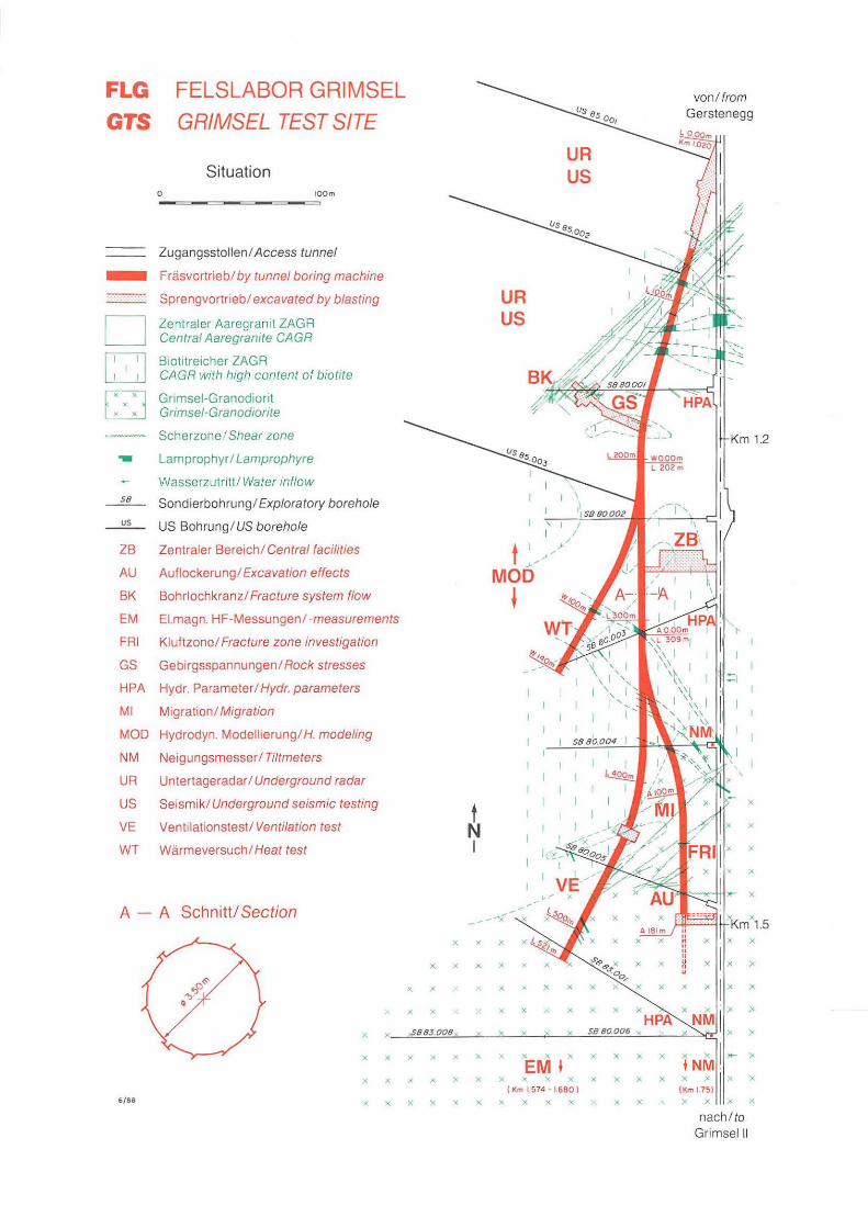
FELSLABOR GRIMSEL
GRIMSEL TEST SITE
Situation
Zugangsstollenl Access tunnel
Fräsvortriebl by tunnel boring machine
Sprengvortrieb/ exca vated by blasting
Zentraler Aaregranit ZAGR Central AaregranIte CAGR
Biotitreicher ZAGR CAGR with high content 01 biotIte
Gnmsel-Granodiorit Grimsef-Granodiorite
Scherzonel Shear zone
Lamprophyr I Lamprophyre
Wasserzutrittl Water inflow
Sondierbohrungl Exploratory borehole
US Bohrungl US borehole
Zentraler Bereichl Central laci/ities
Auflockerungl Excavation effects
Bohrlochkranzl Fracture system flow
Etmagn. HF-Messungen/ -measurements
Kluftzonel Fracture zone investigation
Gebirgsspannungenl Rock stresses
Hydr. Parameter I Hydr. parameters
Migration! Migration
Hydrodyn. Modell ierungl H. modeling
Neigungsmesser / Tiltmeters
Untertageradarl Underground radar
Seismik/Underground seismic testing
Ventilationstestl Ventilation test
Wärmeversuch / Heat test
A - A Schnitt! Seetion
X
x x
x x
6/88 x X
x
x x
x x
X X
x x x
x x X
x x x
t N I
UR US
- --;: ........
x x x
x x , x x X
X X
x , x x
EM x x x x
I
UR US
x X
X X
x x
x x ( Km 1.574 -1 6801
x x x x x
X
X
x
X
x x
von/ (rom Gerstenegg
x x x
x x x
X X X X
X X
X X
,.... x
X X
x x x x
nach/to Grimselll

NAGRA NTB 90-49 - VII-
SUMMARY
From 1987 to 1989 The United States Department of Energy (DOE) and the Swiss Cooperative
for the Disposal of Nuclear Waste (Nagra) participated in an agreement to carry out experiments
for understanding the effect of fractures in the storage and disposal of nuclear waste. As part of this joint work field and laboratory experiments were conducted at a controlled site in the N agra underground Grimsel test site in Switzerland. The primary goal of the experiments in this fractured granite was to determine the fundamental nature of the propagation of seismic waves in
fractured media, and to relate the seismolotgical parameters to the hydrological parameters. The work is ultimately aimed at the characterization and monitoring of subsurface sites for the storage of nuclear waste. The seismic experiments utilized high frequency 1,000 to 10,000 Hz.) signals in a cross-hole configuration at scales of several tens of meters. Two-, three, and foursided tomographic images of the fractures and geologic structure were produced from over 60,000 raypaths through a 10 by 21 meter region bounded by to nearly horizontal boreholes and
to tunnels. Intersecting this region was a dominant fracture zone which was the target of the investigations. In addition to these controlled seismic imaging experiments, laboratory work
using core from this region was performed to establish the relation between fracture content, saturation, and seismic velocity and attenuation. In-situ geomechanical and hydrologiC tests
were carried out to determine the mechanical stiffness and conductivity of the fractures. The results indicate that both P-waves and S-waves can be used to map the location of fractures, both natural and induced from mining activities. In addition, it appears that the frequencies approaching several kilohertz, attenuation measurements are more useful than velocity measure
ments. At lower frequencies the opposite seems to be true. In addition, fractures that are open and hydrologically conductive are much more visible to seismic waves than non-conductive
fractures.

NAGRA NTB 90-49 - VIII-
ZUSAMMENFASSUNG
Zwischen 1987 und 1989 wurde im Auftrag des amerikanischen Energiedepartements (USDOE)
und der Schweizerischen Genossenschaft für die Lagerung radioaktiver Abfalle (NAGRA) ein
Gemeinschaftsprojekt durchgeführt, um den Einfluss von Gesteinsklüften auf die Endlagerung
radioaktiver Abfälle abzuklären. Im Rahmen dieser Zusammenarbeit wurden Feld- und Labor
untersuchungen im Felslabor Grimsel der Nagra durchgeführt. Hauptziel dieser Experimente im
geklüfteten Granit war es, die Ausbreitung seismischer Wellen in geklüfteten Medien sowie den
Zusammenhang zwischen seismischen und hydrologischen Parametern zu untersuchen. Das
generelle Ziel dieser Arbeiten ist es, Methoden für die Charakterisierung und Überwachung von
unterirdischen Standorten für die Lagerung radioaktiver Abfalle zu entwickeln. In den seis
mischen Experimenten wurden Hochfrequenz-Signale (1 '000 bis 10' 000 Hz) in einer
Crosshole-Anordnung über 10-30 Meter eingesetzt. Die Untersuchungen, mit mehr als 60'000
Strahlenwegen, wurden in einem Bereich mit den Dimensionen 10 x 21 Metern durchgeführt,
der einerseits durch zwei nahezu horizontale Bohrlöcher, andererseits durch zwei Stollen
erschlossen ist. Daraus resultieren zwei-, drei- und vierseitige tomographische Abbildungen der
Klüfte, sowie der vorhandenen geologischen Strukturen. Ziel dieser Untersuchungen war die
Charakterisierung einer ausgeprägten Kluftzone, die diesen Bereich durchsetzt. Zusätzlich zu
den seismischen Untersuchungen wurden auch Laborexperimente an Bohrkemen aus diesem
Gebiet durchgeführt, um den Zusammenhang zwischen WassersättigunglFüllung von Kluftzo
nen und seismischer GeschwindigkeitlDämpfung zu bestimmen. In-situ geomechanische und
hydrologische Tests wurden durchgeführt, um die mechanische Steifigkeit und die hydraulische
Konduktivität der Klüfte zu beurteilen.
Die Resultate zeigen, dass sowohl P-Wellen als auch S-Wellen zur Lagebestimmung von natür
lichen und den durch Untertagebau erzeugten Klüften geeignet sind. Es wurde auch festgestellt,
dass für Tomographieuntersuchungen bei Frequenzen im Bereich von mehreren Kilohertz,
Dämpfungsmessungen zweckmässiger sind als Geschwindigkeitsmessungen. Bei niedrigeren
Frequenzen scheint das Gegenteil wahr zu sein. Zudem wurde festgestellt, dass offene und was
serführende Klüfte leichter mit seismischen Wellen zu erkennen sind, als Klüfte die hydraulisch
nicht aktiv sind.

NAGRA NTB 90-49 - IX-
RÉSUMÉ
Dans le cadre d'un accord conclu entre le "Department of Energy" (DOE) des Etats Unis d'Amérique et la "Société coopérative nationale pour l'entreposage de déchets radioactifs (CÉDRA)" suisse, des expériences ont été réalisées entre 1987 et 1989 en vue d'étudier l'effet de fractures dans la roche sur le stockage final de déchets radioactifs. Une partie de ce travail de
coopération a consisté à réaliser des essais de terrain et en laboratoire dans une zone contrôlée du laboratoire souterrain de la Cédra au Grimsel en Suisse. L'objectif principal de ces expérien
ces, dans un massif de granite fracturé, était de déterminer la nature fondamentale de la propagation d'ondes sismiques dans un milieu fracturé et de tirer des relations entre les paramètres
sismiques et les paramètres hydrogéologiques. L'ultime objectif de ces travaux est l'étude et la caractérisation de sites souterrains pour le stockage de déchets radioactifs. Des signaux de haute fréquence (1 '000 à 10'000 Hz) ont été utilisés dans une configuration d'essais entre forages à
des échelles de plusieurs dizaines de mètres. Des images tomographiques des fractures et structures géologiques d'une zone de 10 mètres par 21 mètres, délimitée par deux forages presque horizontaux et deux galeries, ont été élaborées par l'exploitation de plus de 60'000 trajets
d'ondes. Une zone fracturée majeure traversait la région étudiée et constituait la cible de ces investigations. En sus de ces expériences sismiques, des essais en laboratoire sur des carottes
prélevées dans cette zone ont permis l'étude des relations entre la saturation en eau et le remplissage des fractures d'une part, et la vitesse et l'amortissement sismique d'autre part. Des
essais géotechniques et hydrologiques in-situ ont été réalisés afin de déterminer la rigidité mécanique et la conductivité hydraulique des fractures. Les résultats démontrent qu'il est possible d'utiliser aussi bien des ondes P que S pour cartographier les fractures naturelles et celles résultant de travaux d'excavation. Il apparaît en outre que pour des fréquences se situant aux alentours de plusieurs kilohertz, les mesures d'amortissement sont plus utiles que les mesures de vitesse. A fréquences inférieures il semble que c'est le contraire. De plus les fractures ouvertes et perméables sont bien plus visibles pour les ondes sismiques que les fractures étanches.

NAGRA NTB 90-49 -x-
ACKNOWLEDGEMENT
This work was supported through U.S. Department of Energy Contract No. DE-AC03-
76SFOOO98 by the DOE Office of Civilian Radioactive Waste Management, Office of Geologic
Repositories. We also want to thank the personnel at NAGRA and the Grimsel Rock Laboratory for their help and support, in particular Piet Zuidema and Gerdt Sattel, as well as Eric Wys of
SOLEXPERTS AG.

NAGRA NTB 90-49 - XI-
TABLE OF CONTENTS
PREFACE ..................................................................................................................................... II SUMMARy ............................................................................................................................... VII ZUSAMMENF ASSUNG ......................................................................................................... VIII RESUME ..................................................................................................................................... IX ACKNOWLEDGEMENTS .......................................................................................................... X TABLE OF CONTENTS ............................................................................................................. XI LIST OF FIGURES .................................................................................................................. XIII LIST OF TABLES .................................................................................................................... XXI
1.0 INTRODUCTION .......................................................................................................... 1
2.0 GEOLOGIC OVERVIEW OF THE FRI SITE .............................................................. 7
2.1 Introduction .............................................................................................................. 7 2.2 The FRI S-Zone ...................................................................................................... 13 2.3 Lamprophyres ......................................................................................................... 18 2.4 Tension Fissures ..................................................................................................... 19 2.5 Summary ................................................................................................................ 20
3.0 LABORATORY SEISMIC MEASUREMENTS ........................................................ 21
3.1 Introduction ............................................................................................................ 21 3.2 Theory .................................................................................................................... 22 3.3 Specimen Description, Preparation ........................................................................ 25 3.4 Experimental Equipment and Procedures .............................................................. 25 3.5 Results of Laboratory Measurements ..................................................................... 33
3.5.1 Effects of Saturation .................................................................................... 38 3.5.2 Comparison of the Fractured and Intact Samples ....................................... 44 3.5.3 Spectral Analysis of the Fractured Specimen before and after
Wood's Metal Injection ............................................................................... 46
3.6 Sumnlary and Discussion ....................................................................................... 51
4.0 SEISMIC IMAGING EXPERIMENTS ....................................................................... 53
4.1 Introduction ............................................................................................................ 53 4.2 FRI Zone Experimental Procedure ......................................................................... 54 4.3 Data Processing Sequence ...................................................................................... 55
4.3.1 Picking the Travel Times ............................................................................ 56 4.3.2 Inversion ...................................................................................................... 60 4.3.3 Anisotropy Corrections ............................................................................... 71
4.4 Cross Well Studies ................................................................................................. 73 4.5 Amplitude Tomography ......................................................................................... 81 4.6 Discussion of Results ............................................................................................. 87 4.7 Geologic Interpretation of the Results ................................................................... 91

NAGRA NTB 90-49 -XII-
5.0 HYDROLOGIC ANALYSIS OF PRI EXPERIMENT ............................................... 97
5.1 Introduction ............................................................................................................ 97 5.2 Background ............................................................................................................ 97
5.2.1 Constant Pressure VS. Constant Rate Test ................................................... 97 5.2.2 Constant Pressure Solution .......................................................................... 99
5.3 Test Figuration ....................................................................................................... 99 5.4 Test Results and Analysis .................................................................................... 102
5.4.1 Skin ............................................................................................................ 1M 5.4.2 Anisotropy ................................................................................................. 106 5.4.3 Leakage ..................................................................................................... 108 5.4.4 Boundary Effect ........................................................................................ 111
5.5 Conclusions .......................................................................................................... 113
6.0 INFLATION lESTS .................................................................................................. 117
6.1 Introduction ........................................................ , ................................................. 117 6.2 Description of the Experiment ............................................................................. 117 6.3 Deformation Measurements ................................................................................. 124 6.4 Analysis of Deformation Measurements .............................................................. 127 6.5 Seismic Results of Inflation Tests ........................................................................ 142 6.6 Hydrologic Analysis ............................................................................................. 158
7.0 SUMMARY, CONCLUSIONS AND RECOMMENDATIONS .............................. 163
8.0 REFERENCES ........................................................................................................... 169
Appendix A ................................................................................................................................ 171

NAGRA NTB 90-49 - XIII -
Figure 1.1.
Figure 1.2.
Figure 1.3.
Figure 2.1.
Figure 2.2.
Figure 2.3.
Figure 2.4.
LIST OF FIGURES
Regional setting of the Grimsel Rock Laboratory.
Geologic map showing the major structures at the surface above the Grimsellaboratory (from NTB 87-14). The SI zones shown in heavy lines project down to the vicinity of the FRI site.
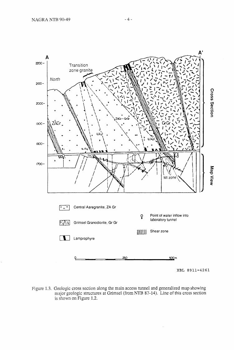
Geologic cross section along the main access tunnel and generalized map showing major geologic structures at Grimsel (from NTG 87-14). Line of this cross section is shown on Figure 1.2.
Map of the southern part of the Grimsellaboratory showing key geologic features and the location of the FRI site. From Nagra Technical Report 87-14.
Geologic map of the FRI site in the plane of boreholes BOFR 87.001 and 87.002. Unmatched lines are fractures. Lamprophyres are marked L. kakirite (cataclasite) zones K, and thin shear bands S, modified from Geotest Report 87048A.
Log of the AU tunnel showing traces of fractures (solid lines), mineralized veins (dashed lines), and other geologic structures exposed in the AU tunnel near the FRI site. Pairs of numbers separated by a slash indicate fracture dip direction and dip. The NE strike of the features is revealed by the orientation of the traces on the tunnel floor. Mineralization key: Q = quartz, F = feldspar, and B = biotite. From preliminary draft ofNTB 87-14.
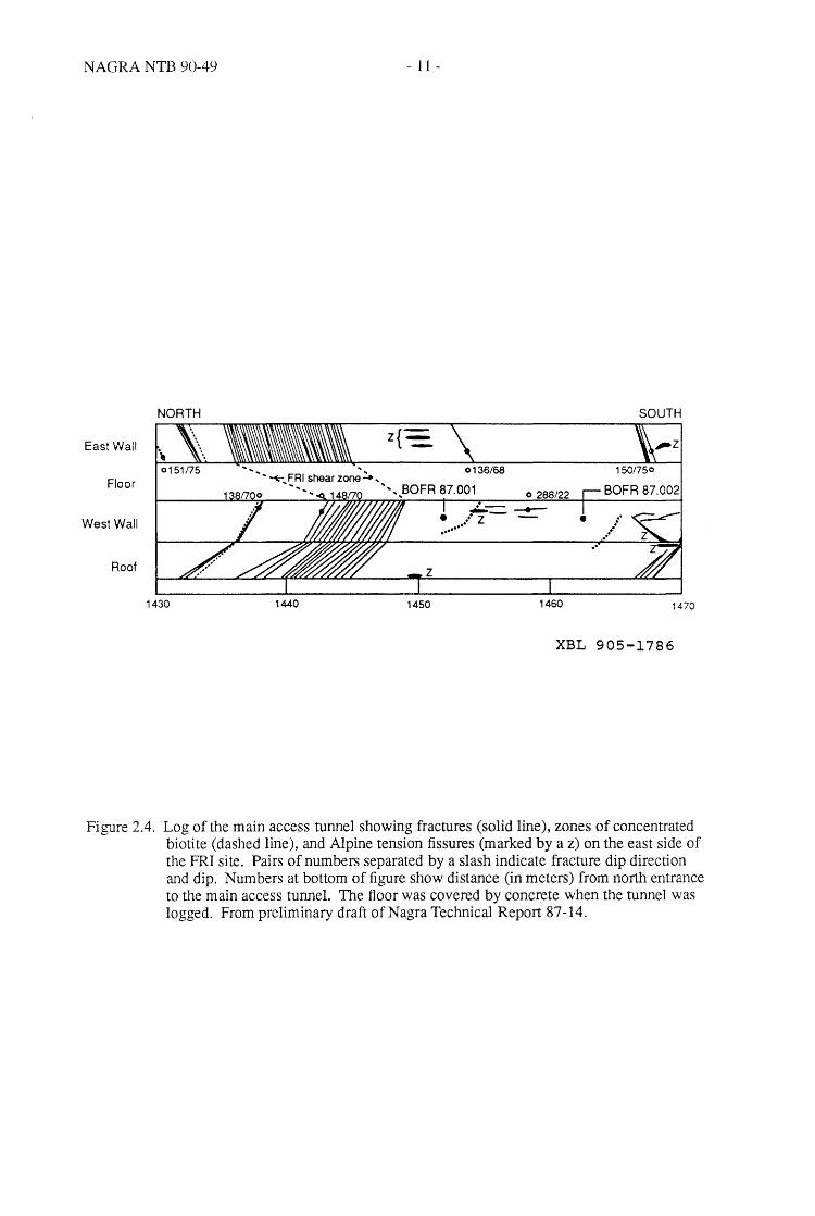
Log of the main access tunnel showing fractures (solid line), zones of concentrated biotite (dashed line), and Alpine tension fissures (marked by a z) on the cast side of the FRI site. Pairs of numbers separated by a slash indicate fracture dip direction and dip. Numbers at bottom of figure show distance (in meters) from north entrance to the main access tunnel. The floor was covered by concrete when the tunnel was logged. From preliminary draft of Nagra Technical Report 87-14.
Page
2
3
4
8
9
10
11

NAGRA NTB 90-49 - XIV-
Figure 2.5a,b. Logs of core from six boreholes (a) BOFR 87.001 and (b) BOFR 14 87.002 at the FRI site. Logs are from Geotest Report 87048A. Explanation for fracture minerals: Q = quartz, E = epidote, Chl = chlorite, B = biotite.
Figure 2.5c,d. Logs of core from six boreholes (c) BOFR 87.003 and (d) BOFR 15 87.007 at the FRI site. Logs are from Geotest Report 87048A. Explanation for fracture minerals: Q = quartz, E = epidote, Chl = chlorite, B = biotite.
Figure 2.5e,f. Logs of core from boreholes (e) BOAU 83.030 and (f) BOAU 16 83.034 at the FRI site. Logs are from a preliminary volume of Nagra Technical Report 87.14. Explanation for fracture minerals: Q = quartz, E = epidote, Chl = chlorite, B = biotite.
Figure 2.6. Schematic diagram showing the braided fracture pattern within 17 northeast-striking shear zones near the Grimsel Rock Labora-tory. The heavy dashed line is a kakirite-bearing fracture. The light dashed lines mm the foliation in the rock.
Figure 3.1. Theoretical prediction of effect of a fracture on velocity and 24 amplitude of transmitted wave; (a) change in pulse for a range of fracture stiffhess; (b) corresponding frequency spectra.
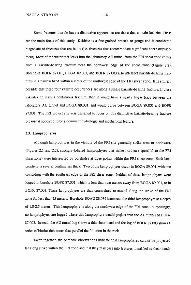
Figure 3.2. Plan view showing the location of specimens tested in the 26 laboratory.
Figure 3.3. Schematic cross section of low frequency transducers used in 28 experiments.
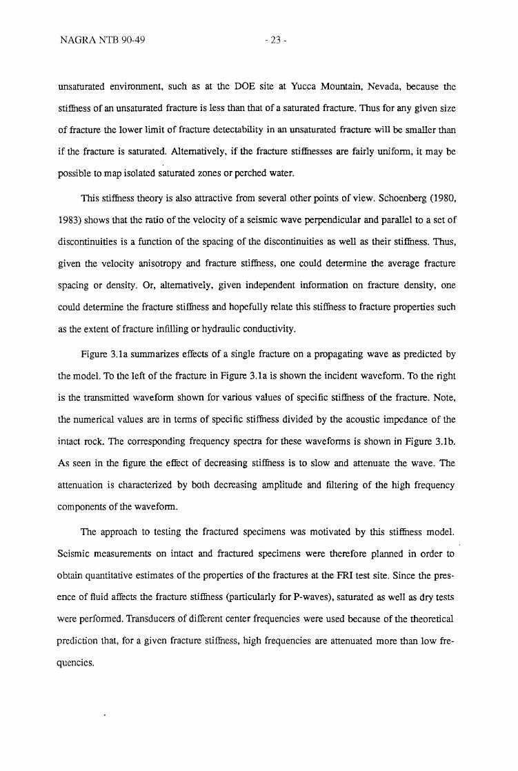
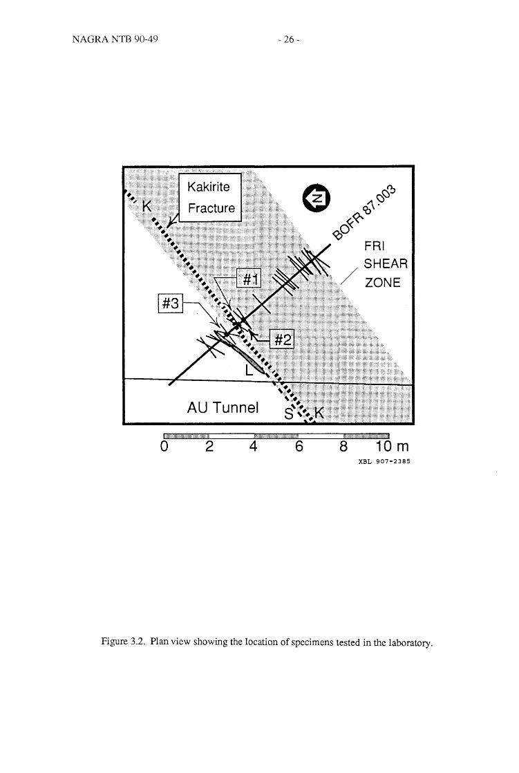
Figure 3.4. Spectra for a test on the aluminum standard using low frequency 30 transducers; (a) P-wave spectrum; (b) S-wave spectrum.
Figure 3.5. Spectra for a test on the aluminum standard using high fre- 30 quency transducers; (a) P-wave spectrum (b) S-wave spectrum.
Figure 3.6. Schematic illustration of experimental setup for seismic meas- 32 urements.
Figure 3.7. Schematic illustration of apparatus for measurements with 32 Wood's metal injection.
Figure 3.8. Example waveforms for intact specimen, ambient conditions, 34 low frequency transducers, 160 kN load level, total travel time of first arrival in /lS; (a) P-wave (b) S-wave.

NAGRA NTB 90-49 -xv-
Figure 3.9. Example waveforms for intact specimen, saturated conditions, 34 low frequency transducers, 160 kN load level, total travel time of first arrival in J.1S; (a) P-wave (b) S-wave.
Figure 3.10. Example waveforms for fractured specimen, dry conditions, low 35 frequency transducers, 160 kN load level, total travel time of first arrival in J.1S; (a) P-wave (b) S-wave.
Figure 3.11. Example waveforms for fractured specimen, saturated condi- 35 tions, low frequency transducers, 160 kN load level, total travel time of first arrival in J.1S; (a) P-wave (b) S-wave.
Figure 3.12. Example waveforms for intact specimen, dry conditions, high 36 frequency transducers, 160 kN load level, total travel time of first arrival in J.1S; (a) P-wave (b) S-wave.
Figure 3.13. Example waveforms for intact specimen, saturated conditions, 36 high frequency transducers, 160 kN load level, total travel time of first arrival in J.1S; (a) P-wave (b) S-wave.
Figure 3.14. Example waveforms for fractured specimen, dry conditions, high 37 frequency transducers, 160 kN load level, total travel time of first arrival in J.1S; (a) P-wave (b) S-wave.
Figure 3.15. Example waveforms for fractured specimen, saturated condi- 37 tions, high frequency transducers, 160 kN load level, total travel time of first arrival in J.1S; (a) P-wave (b) S-wave.
Figure 3.16. Comparison of velocities for ambient and saturated conditions, 39 intact specimens, low frequency transducers; (a) P-wave; (b) S-wave.
Figure 3.17 Comparison of velocities for dry and saturated conditions, frac- 39 tured specimens, low frequency transducers; (a) P-wave; (b) S-wave.
Figure 3.18. Comparison of velocities for dry and saturated conditions, intact 42 specimens, high frequency transducers; (a) P-wave (b) S-wave.
Figure 3.19. Comparison of velocities for dry and saturated conditions, frac- 42 tured specimens, high frequency transducers; (a) P-wave (b) S-wave.
Figure 3.20. Comparison of peak to peak amplitudes for dry and saturated 43 conditions, fractured specimen, low frequency transducers; (a) P-wave (b) S-wave.

NAGRA NTB 90-49 - XVI-
Figure 3.21. Comparison of peak to peak amplitudes for dry and saturated 43 conditions, fractured specimen, low frequency transducers after modifications; (a) P-wave (b) S-wave.
Figure 3.22. Comparison of peak to peak amplitudes for dry and saturated 45 conditions, fractured specimen, high frequency transducers; (a) P-wave (b) S-wave.
Figure 3.23. Comparison of peak to peak amplitudes for dry and saturated 4.5 conditions, intact specimen, high frequency transducers; (a) P-wave (b) S-wave.
Figure 3.24. Comparison of log spectral ratios for P-waves before and after 48 Wood's metal injection at axial loads of (a) 120 kN, (b) 240 kN, and (c) 320 kN.
Figure 3.25. Comparison of log spectral ratios for S-waves before and after 49 Wood's metal injection at axial loads of (a) 120 kN, (b) 240 kN, and (c) 320 kN.
Figure 4.1. Typical example of the crosshole 1987 P-wave data acquired at 57 the FRI zone.
Figure 4.2. Typical example of the crosshole 1988 P-wave data acquired at 57 the FRI zone. Shown in both figures are the picked arrival times.
Figure 4.3. (a) 1987 travel time versus distance data; (b) 1987 velocity 58 versus distance data; and (c) 1987 velocity versus incidence angles. The dashed and solid lines are the least square fit of the data for the 1988 and 1987 data respectively, compare to Figure 4.4 for 1988 data.
Figure 4.4. (a) 1988 travel time versus distance data; (b) 1988 velocity 59 versus distance data; and (c) 1988 velocity versus incidence angles. The dashed and solid line is the least square fit of the data for the 1987 data, the solid line is the fit for the 1988 data, compare to Figure 4.3 for 1987 data.
Figure 4.5. The travel time versus station number for the 1987 crosshole 61 data, compare to Figure 4.6a.
Figure 4.6a. Travel time versus station number from the 1988 crosshole paths 61 for rays actually used in the final inversion.

NAGRA NTB 90-49 -XVII-
Figure 4.6b. The travel time versus stations number for rays from BOFR 62 87.002 to the laboratory tunnel.
Figure 4.6c. The travel time versus station number for rays from BOFR 62 87.001 to the laboratory tunnel.
Figure 4.6d. The travel time versus station number for rays from BOFR 63 87.002 to the access tunnel.
Figure 4.6e. The travel time versus station number for rays from BOFR 63 87.00 1 to the access tunnel.
Figure 4.7a. Waveform data from ray paths BOFR 87.001 to the access tun- 64 nel. These are unusual rays that were not used in the final inver-sion. Note the shift in the data at the top and bottom of the figure. Total time shown is 8.2 millimeters with each time line 1.0 milliseconds. The traces are for station 329 (top) through 253 (bottom) at 0.5 meter intervals.
Figure 4.7b. Waveform data from ray paths BOFR 87.(X)1 to the access tun- 65 nel. These were not deleted from the final version of the tomo-gram.
Figure 4.7c. Waveform data from ray paths BOFR 87.002 to the access tun- 66 nel. These were the unusual rays that were not used in the final inversion. Note the shift in the data at the top and bottom of the figure.
Figure 4.7d. Waveform data from ray paths BOFR 87.002 to the access tun- 67 nel. These were not deleted from the final version.
Figure 4.8. The final result of inverting all the good data from the 1987 tests. 69
Figure 4.9. The final result of inverting all of the good data from the 1988 70 tests. No arusotropic corrections, "unusual" ray paths deleted.
Figure 4.10. The final 1987 inversion after correcting for anisotropy. 74
Figure 4.11. The final 1988 inversion after correcting for arusotropy. The 75 "unusual" rays have been deleted.
Figure 4.12. Cross borehole data inversion of 1987 data, no anisotropy 77 correction.
Figure 4.13. Cross borehole data inversion of 1988 data, no anisotropy 78 correction.

NAGRA NTB 90-49 - XVIII-
Figure 4.14. Cross borehole data from 1987 which was corrected for aniso- 79 tropy and inverted.
Figure 4.15. Cross borehole data from 1988 which was corrected for aniso- 80 tropy and inverted.
Figure 4.16. Measured radiation pattern of the 1988 source. 83
Figure 4.17. Result of inverting the 1988 amplitude data. 85
Figure 4.18. Result of inverting the 1988 cross borehole amplitude data. 86
Figure 4.19. Difference between the 1988 and 1987 tomograms after aniso- 89 tropy corrections.
Figure 4.20. (a) The velocity tomogram for 1988 compared to (b) the geolo- 92 gic map of the FRI site.
Figure 5.1. Dimensionless head at rD = 10, 30, and 100. 100
Figure 5.2. Dimensionless flow at the well. 100
Figure 5.3. Packer locations used in Tests 1,2 and 3 as of August 1988. 101
Figure 5.4. Interference buildup data for Test 1 at various observation 103 points.
Figure 5.5. Comparison between data and the theoretical response curve. 103
Figure 5.6. Type curve match with the skin curves. 105
Figure 5.7. Type curve match assuming the lower injection head of 6.6 bars. 105
Figure 5.8. flow rate decline curve. Also shown are the decline curves for 107 various values of s observed at 11.2.
Figure 5.9. Dimensionless pressure at various rD and the equivalent aniso- 109 tropy ratio.
Figure 5.10. Type curve match of the flow rate with Da Prat et al. solution. 110
Figure 5.11. Type curve match of the pressure at 13.1 with Da Prat et al. solu- 110 tion.

NAGRA NTB 90-49 - XIX-
Figure 5.12. Type curve match at 13.1 with a leaky fracture zone solution. 112
Figure 5.13. Type curve match at 11.2 with a leaky fracture zone solution. 112
Figure 5.14. Numerical model of the FRl fracture a) with and b) without tun- 114 nels.
Figure 5.15. Simulated data for the pressures at 13.1. 115
Figure 5.16. Simulated data for the flow rntes at 11.2. 115
Figure 6.1. Bofex instrumentation for fracture displacement measurements. 118
Figure 6.2. Plan view showing instrumentation locations for inflation test. 120
Figure 6.3. Time line of events in inflation test and pressure history in inter- 122 vals 11.2 ofBOFR 87.001 and 13.1 ofBOFR 87.003.
Figure 6.4. (a) Pressure history in interval 11.2, BO 87.001, during inflation 125 test; (b) fracture displacements as measured by Bofex 1 in BO 87.001 during inflation test. Vertical dashed lines show coin-cidence in time of events.
Figure 6.5. (a) Pressure history in interval 13.1, BO 87.003, during inflation 126 test; (b) fracture displacements as measured by Bofex 3 in BO 87.0003 during inflation test. Vertical dashed lines show coin-cidence in time of events.
Figure 6.6. Modelling the inflation experiment by a pressurized crack with 129 stiffuess. Assuming elasticity, model 1 is decomposed into two simple models designated II and III.
Figure 6.7. Displacement as a function of distance from the midpoint of the 131 crack in element II, assuming 1= 13.62 m and crack lengths from 20 to 1000 m.
Figure 6.8. Predicted fracture stiffuess as a function of crack length. 134
Figure 6.9. DefOImation between two points located 0.75 m either side of 136 the midpoint of the center crack of a row of pressurized coplanar cracks.
Figure 6.10. Nonnalized contact area of fracture faces as a function of crack 136 half spacing b for a defonnation of 1.42 x 10⁻⁶m.

NAGRA NTB 90-49 -xx-
Figure 6.1l. Magnitude of the transmission coefficient and nonnalized group 138 delay for a seismic wave nonnally incident upon a displacement discontinuity as a function ofnonnalized frequency.
Figure 6.12. Typical results of laboratory measurement of stiffness of the 141 fracture in fractured specimen #2; (a) change in volume of water in the fracture during loading and unloading, (b) stiffness based on volume change measurements.
Figure 6.13a. Recorded wave fonn data for component 1 prior to inflation test 144 in 87.001.
Figure 6.13b. Recorded wave fonn data for component 2 prior to inflation test 145 in 87.001.
Figure 6.13c. Recorded wave fonn data for component 3 prior to inflation test 146 in 87.001.
Figure 6.14a. Recorded wave fOIm data for component 1 after fracture had 147 been pressurized to 20 bars in 87.001 for two days.
Figure 6.14b. Recorded wave fonn data for component 2 after fracture had 148 been pressurized to 20 bars in 87.001 for two days.
Figure 6.14c. Recorded wave fonn data for component 3 after fracture had 149 been pressurized to 20 bars in 87.001 for two days.
Figure 6.15. Amplitude versus station number for the unpressurized data. 150 (dark squares), and after 2 days of pressurization, (open squares) for (a) component 1, (b) component 2, and (c) component 3.
Figure 6.16. Amplitude values for data given in Table 6.2 for (a) component 152 1, (b) component 2, and (c) component 3.
Figure 6.17. The relative attenuation between measurements for the values in 154 Table 6.2, measurement 1 is taken as baseline. All three com-ponents have been averaged to obtain the amplitude values.
Figure 6.18. Amplitude values for a data given in Table 6.3 (a) component 1, 157 (b) component 2, and (c) component 3.
Figure 6.19. Flow rate into 11.2 during injection. 160
Figure 6.20. Injectivity (QIP) of BOFR 87.001 during the inflation test. 161
Figure A.I. HV pulser system 172
NAGRA NTB 90-49 - XXI-
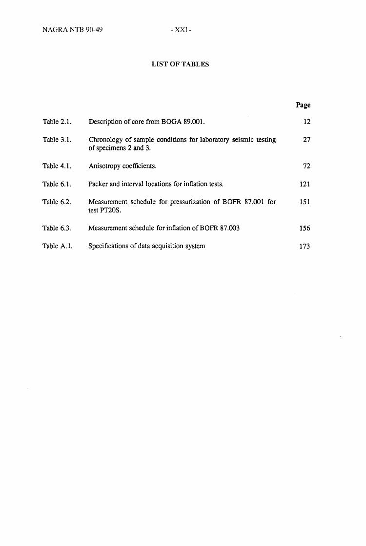
LIST OF TABLES
Page
Table 2.1. Description of core from BOGA 89.001. 12
Table 3.1. Chronology of sample conditions for laboratory seismic testing 27 of specimens 2 and 3.
Table 4.1. Anisotropy coefficients. 72
Table 6.1. Packer and inteIVallocations for inflation tests. 121
Table 6.2. Measurement schedule for pressurization of BOFR 87.001 for 151 test PT20S.
Table 6.3. Measurement schedule for inflation ofBOFR 87.003 156
Table A.l. SpeCifications of data acquisition system 173


NAGRA NTB 90-49 - 1 -
1.0. INTRODUCTION
The Swiss National Cooperative for the Disposal of Radioactive Waste (Nagra) has hosted
and carried out a variety of experiments at the underground Grimsel Rock Laboratory near the
Grimsel Pass in the Swiss Alps (Figures 1.1, 1.2, and 1.3). From 1987 through 1989 the U. S.
Department of Energy (DOE) has participated in an agreement with Nagra to perfonn joint
research on various topics related to geologic storage of nuclear waste. As part of this Nagra
DOE Cooperative (NDC-I) project Lawrence Berkeley Laboratory (LBL) has participated in
several projects at Grimsel which are directed towards improving the understanding of the role of
fractures in the storage of nuclear waste. This report describes a series of experiments at Grimsel
called the Fracture Research Investigation (FRI). The FRI project has been designed to address
the effects of fractures on the propagation of seismic waves and the relationship of these effects
to the hydrologic behavior.
It is necessary to locate and characterize fractures to accurately model the hydrological and
geomechanical behavior of geologic repositories. Although fracture properties can be observed
directly at the surface, in underground openings, and from boreholes, a vast majority of the rock
can not be examined directly. Because almost all rock is heterogeneous, one can not rely on the
simple interpolation or extrapolation of structural information for adequate fracture characteriza
tion. Unobserved features within a rock body may playa dominant role in its geomechanical or
hydrologic behavior. Therefore, there is a crucial need to have techniques for fracture detection
and characterization between boreholes and underground openings.
The FR.I work was aimed at developing practical borehole seismic and hydrological
methods for use during the characterization and monitoring of underground nuclear waste facili
ties. The fundamental design of the project was to find a simple, well defined, accessible fracture
zone surrounded by relatively unfractured rock and use this zone as a point of comparison for

NAGRA NTB 90-49 - 2 -
• ZUrich
Miles 5 0 5 10 20 30 40 50
Kilometers 5 0 5 10 20 30 40 50 60
XBL 899-6312
Figure 1.1. Regional setting of the Grimsel Rock Laboratory.

NAGRA NTB 90-49
Legend -- Main access tunnel ~ and Laboratory tunnels
- 3 -
-._.- S1 -- - K 2 ----- Lamprophyre ··_··-S2
··········S3 Scale
o 50 100 200 300 meters
XBL 905-1782
Figure 1.2. Geologic map showing the major structures at the surface above the Grimsellaboratory (from NTB 87-14). The Sl zones shown in heavy lines project down to the vicinity of the FRI site.
NAGRA NTB 90-49
22CO-
21CO-
19:>0-
1800-
1700-
1+ + + I Central Aaregranite, ZA Gr
~ Grimsel Granodiorite, Gr Gr
[J] Lamprophyre
9
- 4-
250
Point of water inflow into laboratory tunnel
1111111111111 Shear zone
AI
XBL 8911-4261
Figure 1.3. Geologic cross section along the main access tunnel and generalized map showing major geologic structures at Grimse1 (from NTB 87-14). Line of this cross section is shown on Figure 1.2.
(")
'"" o fJ) fJ)
en <D o =: o :J

NAGRA NTB 90-49 - 5 -
seismic, hydrologic and mechanical behavior. The FRI site was designated in the Grimsel Rock
Laboratory for this purpose and field work was carried out during each year of the three year
NDC-I project (1987-1989). The FRI project has involved separate and simultaneous, detailed
geologic studies, field measurements of seismic wave propagation, geomechanical measurements
of fracture properties, and the hydrologic response of the fractured rock. Laboratory measure-
ments of core have also been carried out to address the fundamental nature of seismic wave pro-
pagation in fractured rock. Because all these studies were focussed on the same fracture zone, the
study provided insight into
• New theories of seismic wave propagation through fractures,
• How changes in the fracture properties affect seismic wave propagation,
• Interpretation of seismic tomography to identify hydrologic features, and
• Integration of seismic data into a hydrologic testing plan.
The FRI work was interdisciplinary with the strongest emphasis on seismic imaging. Com-
pared to other efforts the seismic measurements were most extensive and comprehensive. The
hydrologic measurements were not as complete and although the laboratory studies of the
seismic properties of cores was reasonably comprehensive f the in situ mechanical measurements
were only prototypes. This scheme was appropriate for the FRI site, because the fracture zone is
well exposed in the two parallel drifts which intersect it, therefore it seemed clear that the hydrol-
ogy of the site would be mainly confined to the fracture zone. Because of this the number one
focus of the work was to evaluate and develop seismic methods to provide information about
hydrologic properties in a fractured rock environment.
As the work progressed, it followed the course of most projects in L;e earth sciences in that
as our understanding of the rock increased, the "simple" fracture zone became more complex. It .
is natural in such cases to plan for a follow up validation exercise where new holes would be
drilled to obtain direct observations of features predicted by the geophysical interpretation and
more extensive hydrologic testing would be conducted to determine the hydrologic role of these
features. Although this effort could not be accommodated withing the NDC-I project, the authors
feel that such efforts would be elucidating. This is an unnecessary page for all but the computer.

NAGRA NTB 90-49 - 6 -
Overall the project is a unique effort in combining several different disciplines to define a com
plex problem.

NAGRA NTB 90-49 - 7 -
2.0. GEOLOGIC OVERVIEW OF THE FRI SITE
2.1. Introduction
The FRI site is located in the southern part of the Grimsel Rock Laboratory (Figure 2.1) and
is bounded on the west by the AU laboratory tunnel, on the east by the main access tunnel, and
on the north and south by boreholes BOFR 87.001 and BOFR 87.002 respectively (Figure 2.2).
The FRI site lies within the Grimsel Granodiorite, close to a very irregular contact with the
lighter-colored Central Aaregranite. The eastern parts of the cores from the two boreholes bound
ing the site are distinctly lighter in color than the western parts of the cores. This color change
may reflect differences in hydrothermal alteration across the site, variation in the original
mineralogy of the grandiorite, or the presence of lenses of Central Aare granite. Both the Grimsel
Grandiorite and the Central Aareganite are foliated. The foliation strikes northeast, and dips
steeply to the southeast. It is defined by aligned grains of biotite and bands of mylonite. A
steeply-plunging linear fabric element within the foliation is defined by aligned and elongated
feldspar grains.
Of the many different rock structures at Grimsel, four are hydrologically dominant: S-zones,
K-zones, lamprophyres, and tension fissures (NTB 85-46). The S-zones are fracture-bearing shear
zones that generally dip steeply to the southeast, parallel to the foliation in the host rock. Within
the S-zones, both the fractures and the grain-scale mineral fabric of the rock dip steeply to the
southeast. The K-zones are fracture zones that generally strike west or northwest; they cut the
host rock fabric at a high angle. The lamprophyres are mafic igneous dikes. They dip steeply and
generally strike west or northwest. These have been metamorphosed and contain abundant
biotite. The lamprophyres are highly discontinuous and are widely distributed at Grimsel. Ten
sion fissures are subhorizontal and usually filled with quartz crystals and chlorite. S-zones, lam
prophyres, and tension fissures are exposed in the tunnels bounding the FRI site (Figures 2.3 and
2.4).

NAGRA NTB 90-49
Cable Tunnel
ZAGr
Scale
o 50 meters
- 8 -
-FRI Site
_ en 400.00 m=-\"", CD --
Laboratory ~ - _ \ Tunnel g ZAGr \
- -~ - ~,\
~
Legend
Petrography D Central Aaregranite (ZAGr)
I I ZAGr, biotite rich
Fractured Zones
Water
[SJ Grimsel Granodiorite (GrGr)
.. Lamprophyre
EI}:}I Regions with Lamprophyre
,....,..,., Shear Zone
I I Strongly fractured zone
II Evidence of water flowing from fractures
.. Localized flow> 0.1 I/min
0.3 (85) Flow in I/min (year)
v U-rich fluorescence
XBL 905-1783
Figure 2.1. Map of the southern part of the Grimsellaboratory showing key geologic features and the location of the FRI site. From Nagra Technical Report 87-14.

NAGRA NTB 90-49 - 9 -
1450 1460 --~ --- --- --- --- --r
Main Access Tunnel
, ?, Lighter-colored
•••••• ! Ii.............. i .• ~~;Rl:L '? " ? granodiorite "? ",
...-o o
" co cr: I.L o CD
?, Darker-colored
6$§§>;S '''2 6 8* 10m XBL 905-1784
Figure 2.2. Geologic map of the FRI site in the plane of boreholes BOFR 87.001 and 87.002. Unmatched lines are fractures. Lamprophyres are marked L. kakirite (cataclasite) zones K, and thin shear bands S, modified from Geotest Report 87048A.

NAGRA NTB 90-49
o L{) T""'
«
- 10-
.r::. .... ::J o
CJ)
~~~~~~~~~~~lr Q) c::: o N '-ctS Q)
.J::. en
a: LL
--+--+--7trr----+--+----.~ ..L ..... --. .... . ...
a:l. , .... -•••• : ••• # LL···· .. ·,-' ...... , • .. LL .. t !:.. ... d··': ..... . '._ ... O~--------~--+-----~.-.~
o ..... : .. :::: .... ;:::; ........ ' .. ~~--~~~----~------~----~------~ T""' '. ' .. «
- ~ 0 0 ~ a: ....
(f)
co w
'-0 0
LL
-o o a:
.r::. 1::: o Z
Figure 2.3. Log of the AU tunnel showing traces of fractures (solid lines), mineralized veins (dashed lines), and other geologic structures exposed in the AU tunnel near the FRI site. Pairs of numbers separated by a slash indicate fracture dip direction and dip. The NE strike of the features is revealed by the orientation of the traces on the tunnel floor. Mineralization key: Q = quartz, F = feldspar, and B = biotite. From preliminary draft ofNTB 87-14.
NAGRA NTB 90-49
NORTH
East Wall '\ o151n5
Floor
West Wall
Roof
1430
- 11 -
z{-=.
........ ~ FAI shear zo~ ~.. 0136/68
.... .. ...... BOFR 87.001 o 288/22
... -= ----• .•. ··Z -......
1440 1450 1460
SOUTH
BOFR 87.002 . .' .......
.'
1470
XBL 905-1786
Figure 2.4. Log of the main access tunnel showing fractures (solid line), zones of concentrated biotite (dashed line), and Alpine tension fissures (marked by a z) on the east side of the FRI site. Pairs of numbers separated by a slash indicate fracture dip direction and dip. Numbers at bottom of figure show distance (in meters) from north entrance to the main access tunnel. The floor was covered by concrete when the tunnel was logged. From preliminary draft of Nagra Technical Report 87-14.

NAGRA NTB 90-49 - 12 -
Depth em)
0.00-4.50
4.50 -4.85
4.85 - 8.56
Table 2.1. Description of core from BOGA 89.001
Description
Grimsel Granodiorite, moderately dark, medium- to coarse-grained, nonuniform grains, distinct foliation
Zone with sealed quartz-filled fractures; quartz filling shows distinct cracks
Grimsel Granodiorite, moderately dark, medium- to coarse-grained, nonuniform grains, distinct foliation
At 7.73 m is a kakirite zone 5-10 cm thick
8.56 - 9.00 Zone of numerous fractures in part filled with fault gouge
9.00 - 11.43 Grimsel Granodiorite, moderately dark, medium- to coarse-grained, nonuniform grains, distinct foliation
11.43 - 11.76 Grimsel Granodiorite, moderately dark, medium- to coarse-grained, nonuniform grains, intensive mylonitization
11.76 - 11.84 Grimsel Granodiorite, moderately dark, medium- to coarse-grained, nonuniform grains, distinct foliation
11.84 - 11.95 Lamprophyre, biotite-rich, foliated, fractured along foliation
11.95 - 15.73 Grimsel Granodiorite, moderately dark, medium- to coarse-grained, nonuniform grains, distinct foliation, feldspars are saussuritized (chemically altered)
15.73 - 15.80 Lamprophyre, biotite-rich, foliated, fractured along foliation
15.80 - 20.54 Grimsel Granodiorite, moderately dark, medium- to coarse-grained, nonuniform grains, distinct foliation, feldspars are distinctly saussuritized, quartzrich

NAGRA NTB 90-49 - 13 -
Seven main boreholes (Table 2.1 and Figure 2.5) have been drilled and logged at the FRI
site to investigate the zone. Two parallel boreholes (BOFR 87.001 and 87.002) connect the two
tunnels and bracket a section of the FRI shear zone. Borehole BOFR 87.003 was drilled across
the shear zone and borehole BOFR 87.004 was drilled along the northwest edge of the shear
zone. Borehole BOGA 89.001 was drilled after the field investigations reported here were com
pleted. In addition to the main boreholes, a series of small holes were drilled 25 em apart in the
AU tunnel and in the main access tunnel between BOFR 87.001 and 87.002 for emplacing instru
ments for the seismic tomography experiments at the site.
2.2. The FRI S-Zone
This site was chosen for testing because it intersects a prominent S-zone (Figure 2.2). This
S-zone is 5 meters thick and is the most prominent structure at the FRI site. It strikes northeast
and dips steeply to the southeast. The FRI tests were sited at this S-zone because it was con
sidered to have a relatively simple and predictable structure, characteristics which would be an
asset in conducting the various tests planned for the project The leakage of water from the shear
zone indicates that it is hydrologically active.
Fractures in the FR.I borehole cores are most numerous where the foliation in the S-zone is
best developed. In some places where the rock contains fractures it is schistose. Many of the
fractures in the borehole cores occur at edges of mylonite bands which help define the ductile
fabric of the shear zone. The planar anisotropy of the rock in the shear zone thus strongly con
trols the position and orientation of the fractures in the zone.
The S-zone does not consist of parallel fractures, but rather a network of fractures that fonn
a braided pattern (Figure 2.6). Thus, the zone as a whole strikes '"N49°E, but internal fractures
range in strike from N38°E to N52°E. Fracture dip measurements range from 65° to 88° to the
southeast. Most of the fractures have similar appearances, similar orientations, and may be
noticeably nonplanar. Although in general it is difficult to correlate individual fractures from
borehole to borehole, narrow interconnected networks of fractures appear to extend between
boreholes.

a I
DEPTH (meters) 1 I . 5 • T • • 10 " If II .. II II IT " .. 10 II
Pt::TROlOGY /' ,/~~/ ,,:..""l /~ rJll// // L--;W ~1);;' I~:T / ·1111 // . hP A'Y'/' ~ ;~ . /." :
FOl~TlOD 0rGt WITH , ... "VDRO{.
1 ONE ISSt(; GrGf
I 0<0< WIT" ~UI,RtN; 9OIoIE QUARTZ· AND
i TIlE"'AlLJ FElSPNI·RICH ZONES LAl~Dr"
FElDSPAR . RICH ¥E1H9
FRACTURES Without mineral fillings .i,V " / ,'~ / " " // //r // ",
STRIKE DIP " . " //" "7 .' / ,,~ /7; L / "
0 ,/ 0".31)" ,,"" I ... • I I .J'" // .. .,,"'~ " ~ , " - /-,:, . .t? / / ~3I)"-eo"
With mineral fillinas \ , /' ,., /'/ " . ,'- '-, " /,11' ,/ r "'~>
Fracture·filling minerals ( "" . . co, ,...~ 0' c~( Q ew Of .. ~ CN~CMC" • r Q
,.. 10".110' ew
Mineral-fillina tbickness Imm) . . . , . Is • . 10' 40 . . , I
'" tt11 I 10 I
b DEPTHirreNI'Sl
10 II 13 IT " .. ZO It
PETROLOGY
FRACTURES STRII<E o DIP
,/ 0".31)"
~3I)"-eo"
,.. 10".10"
Without minerallillings
With minerallillinas
Frac1ure·lilling minerals
Mineral-fillina thickness (mm)
'-LiT-TiT/? W;j~ ?/ (/;/1'. / .. ~~/ \ ~' ## A_~ 'f #1/:' ./·/_,{.~t;~/~":'1'''.· STRONGlY FOl~TED 0r0r WITH 0r0r WITH SCRtEREN N<O QUARTZ· AHO FELDSPAR- ,WEAK HYDAO'I' FELOIIPARPOAPHYAOIUITI AtCHYEMN<OFIUtCT\JllEII I :1HE_ :
'AlTERATION I
.k'.:~-;~~./'.,P- ..R'Y V//., it,,' ./ ~~.'..:' ~~7/::!;.'~/~~--7T~~r .', .. ,
/ .--> ~7 -1/ Lr ,"-'-- ?'7'7T /71 ,',$
~~~~----. Ci<
~- -..--y
...... ':.:s:. ..
"'-......... ((QI I I .111111111 _
\ . /1 I
to
• ,'.. // /~~~ I~;i ,,' l'·! -,'l i' ~
: WEAK
: FOl~TION I
XBL 905-1787
Figure 2.5a,b. Logs of core from six boreholes (a) BOFR 87.001 and (b) BOFR 87.002 at the FRI site. Logs are from Geotest Report 87048A. Explanation for fracture minerals: Q = quartz, E = epidote, ChI = chlorite, B = biotite.
z >a ~ >z g 1..0 o
I
~ 1..0
>-' ~

c
PETROLOGY
FRACTURES STRIKE o
d
DIP
~ 0"-30"
",( 30"«1"
"" fI(1'«I"
Without mineral fillinos
DEPTH (meters) 01 oz 0.3 04 O~ 01 07 O. 0.1 ..0 1.1 1.1 1.3 1.4 l5 1& J I
PETROLOGY Inc::..-::-/---- -------p .. --t'l~- ..... --:b- IlJlHH - -- --__ .)f
7:"E -.-:,-:,-::..::.;.-:::,:, 4 __ :_-_~ • _ _ ---_ Ji1Ji III WITH 2-5 Mj THICK KAKIRITE SOME
CORE LOSS
XBL 905-1789
Figure 2.5e,d. Logs of core from six boreholes (c) BOFR 87.003 and (d) BOFR 87.007 at the FRI site. Logs are from Geotest Report 87048A. Explanation for fracture minerals: Q = quartz, E = epidote, Chl = chlorite, B = biotite.
z ~ a ~ >z g \0 o ~ \0
-' u.

e 0 I 2 3 , DEPTH (meters)
PETROLOGY E
MILDLY FOliATED GlGr
FRACTURES Without mineral fillings STRIKE DIP
",'" o ~~.~ With mineral fillings ,/ ,,( 30"-60"
Fracture-filling minerals 0 W E
"I 60"-90"
Mineral-filling thickness (mm) .HIO 1 S -~--
f
DEPTH (meters) 0 I ~ ~ I
PETROLOGY
~-~ E
MILDlY FOliA TED GlGr
Willi STRONGLY
FOliA TED LAMPAOPHYRE
FRACTURES Without mineral fillings --~~
STRIKE DIP - //lYJA'g§1 I
0 / 0"-30" '" _?,' I
With mineral fillings __ ......... , "." I
,,( 3O"-W .". //,"'" // " Fracture-filling minerals o 0 00 0 A 60"-110" ( E)
Mineral-fillino thickness (mm) 60-220 5-20 5-15
10-15 10-30
XBL 905-1788
Figure 2.5e,f. Logs of core from boreholes (e) BOAU 83.030 and (f) BOAU 83.034 at the FRI site. Logs are from a preliminary volume of Nagra Technical Report 87.14. Explanation for fracture minerals: Q = quartz, E = epidote, Chl = chlorite, B = biotite.
z )-a ~ )-
z ,..., to \.0 o
I
~ \.0
~
0\

NAGRA NTB 90-49 - 17 -
XBL 903-782
Figure 2.6. Schematic diagram showing the braided fracture pattern within northeast-striking shear zones near the Grimsel Rock Laboratory. The heavy dashed line is a kakiritebearing fracture. The light dashed lines mark the foliation in the rock.
NAGRA NTB 90-49 - 18 -
Some fractures that do have a distinctive appearance are those that contain kakirite. These
are the main focus of this study. Kakirite is a fine-grained breccia or gouge and is considered
diagnostic of fractures that are faults (i.e. fractures that accommodate significant shear displace
ment). Most of the water that leaks into the laboratory AU tunnel from the FRI shear zone comes
from a kakirite-bearing fracture near the northwest edge of the shear zone (Figure 2.2).
Boreholes BOFR 87.CX)1, BOGA 89.001, and BOFR 87'(X)3 also intersect kakirite-bearing frac
tures in a narrow band within a meter of the northwest edge of the FR1 shear zone. It is entirely
possible that these four kakirite occurrences are along a single kakirite-bearing fracture. If these
kakirites do mark a continuous fracture, then it would have a nearly linear trace between the
laboratory AU tunnel and BOGA 89.001, and would curve between BOGA 89.001 and BOFR
87.001. The FR1 project site was designed to focus on this distinctive kakirite-bearing fracture
because it appeared to be a dominant hydrologic and mechanical feature.
2.3. Lamprophyres
Although lamprophyres in the vfcinity of the FRI site generally strike west or northwest,
(Figures 2.1 and 2.2), strongly-foliated lamprophyres that strike northeast (parallel to the FR!
shear zone) were intersected by boreholes at three points within the FRI shear zone. Each lam
prophyre is several centimeters thick. Two of the lamprophyres occur in BOGA 89.001, with one
coinciding with the southeast edge of the FR! shear zone. Neither of these lamprophyres were
logged in borehole BOFR 87.0Cll, which is less than two meters away from BOGA 89.001, or in
BOFR 87.003. These lamprophyres are thus constrained to extend along the strike of the FRI
zone for less than 15 meters. Borehole BOAU 83.034 intersects the third lamprophyre at a depth
of 1.0-2.5 meters. This lamprophyre is along the northwest edge of the FR.! zone. Surprisingly,
no lamprophyres are logged where this lamprophyre would project into the AU tunnel or BOFR
87.003. Instead, the AU tunnel log shows a thin shear band and the log of BOFR. 87.003 shows a
series of biotite-rich zones that parallel the foliation in the rock.
Taken together, the borehole observations indicate that lamprophyres cannot be projected
far along strike within the FR.! zone and that they may pass into features identified as shear bands

NAGRA NTB 90-49 - 19 -
or biotite-rich zones. The northeast strikes of these lamprophyres are anomalous; most of the
lamprophyres exposed in the AU tunnel and at the surface strike west or northwest. These
findings are consistent with the northeast-striking lamprophyres having been stretched out along
the FR.I zone during shear deformation in the geologic past. Stretching could account for the
apparently discontinuous nature of FRl lamprophyres, their strong foliation, and their zone
parallel strikes. Interestingly, the FRI lamprophyres seem most common where the foliation and
fracturing within the zone is most extensively developed, near the edges of the FR! shear zone.
West-striking lamprophyres at the FR! site are logged in the AU tunnel but none have been
logged in the main access tunnel. Some might intersect the main access tunnel and yet not be
logged, for the blocky nature of the main access tunnel makes logging difficult. However, the
lamprophyres might also pinch out within the FRI site or be offset across the FRI shear zone. As
an example, the lamprophyre exposed in the AU tunnel near the mouth of borehole BOGA
89.001 apparently pinches out before reaching the hole.
2.4. Tension Fissures
Many gently-dipping Alpine tension fissures (ZerrkIll/te) occur in the southern part of the
laboratory. Most of tl1e exposed fissures have apertures of several centimeters, but some fissures
that are several meters long have apertures that locally exceed a meter. The fissures commonly
occur near lamprophyres. A fissure exposed in the AU tunnel at A148 (Figure 2.3) may extend
from a lamprophyre along the SE margin of the FRI shear zone (Figure 2.2). A cluster of gently
dipping fissures near the 1450-meter mark of the main access tunnel occur near a biotite-rich area
that may be associated with a lamprophyre (Figure 2.4). Borehole BOFR 87.001 encounted a .
gently-dipping, quartz-filled fracture within the FRI site, approximately 12.8 meters from the
laboratory AU tunnel. This fracture is not far from the more westerly lamprophyre encountered
in BOGA 89.001. In addition to the fissures that are associated with the lamprophyres, several
gently-dipping fractures that appear to be distant from lamprophyres have been logged in the AU
tunnel at the west side of the FRI site. Given the number of gently-dipping fissures encountered
near the FR.I site, it would not be surprising if more occurred within it

NAGRA NTB 90-49 - 20-
2.5. Summary
The FR.I project was designed to test the coupled seismic, mechanical, and hydrologic
behavior of a prominent, yet relatively simple fracture. Key goals of the project were to evaluate
and improve our ability to use seismic methods as part of a hydrologic characterization of a frac
tured rock mass. The kakirite-bearing fracture in the shear zone at the PRJ site was the principal
target of the FR.I tests. The distinctive appearance, water-bearing capacity, and general setting
of this fracture indicated that it would be appropriate for our purposes.
Some additional aspects of the geology at the FRI site are expected to bear on the seismic,
mechanicat and hydrologic tests. First, the rock mass at the site is decidedly heterogeneous.
The granitic rock within the site is compositionally nonuniform and contains lamprophyres. Two
objectives of the seismic experiments were to determine whether the lithologic heterogeneity
within the site can be imaged and whether this heterogeneity prevented the kakirite-bearing frac
ture from being imaged. A second important aspect of the rock at the site is its anisotropy, which
locally is quite pronounced. Both the grain-scale fabric of the rock and most of the macroscopic
fractures are preferentially aligned subparallel to planes that dip steeply to the southwest. The
rock also possesses a linear fabric element in which the rock grains are elongated in the direction
of the foliation dip. fluid flow may occur most readily in the direction of the foliation dip
because potential fracture flow paths are least tortuous (Figure 2.6). A final set of important
points regards the structure of the FRI shear zone. Many individual features within the shear
zone are either discontinuous or do not extend far along strike. Because of the braided fracture
pattern with shear zones at Grimsel, the kakirite-bearing fracture on wh.ich we focus may not be
hydrologically isolated. The presence of lamprophyres and gently-dipping fissures, features that
are hydrologically important at many points in the laboratory, may also complicate the hydrology
of the FRI site.

NAGRA NTB 90-49 - 21 -
3.0. LABORATORY SEISMIC MEASUREMENTS
3.1. Introduction
The FRI geomechanical experime~ were designed to sort out the effects rock properties
on the propagation of seismic waves under controlled laboratory conditions. This information
was in tum used to help interpret the tomographic data discussed in Chapter 4. The goals of the
laboratory work were to determine the effects of
• Saturation
• Stress
• Scale • Fracturing
on transmitted compressional and shear waves. The geomechanical tests for FRI encompassed
laboratory seismic testing of intact and fractured core specimens to measure P- and S-wave velo
cities and amplitudes for a range of loads and saturation conditions bracketing the in-situ condi
tions. These data were important for the interpretation of the in-situ seismic measurements.
We were able to complete a fairly extensive study of the first two goals. For the last two
goals, we were able to gain useful insight despite the problems that were encountered. To study
scale effects one core sample was drilled so that the kakirite fracture was oriented along the core
axis. This core was essentially rubble and could not be tested. Had testing been possible, labora
tory hydromechanical and seismic measurements could have been compared with field measure
ments on the same fracture at a much larger scale. Quantitative interpretation of the effects of
fractures on wave propagation was hampered by a high degree of heterogeneity in the rock.
Even though fractured and intact samples were adjacent to one another in the core, the rock
matrix in the intact core was different than the rock matrix of the fractured core. In order to over-
come this problem, one fractured sample was injected with Wood's metal to "erase" the effect of

NAGRA NTB 90-49 - 22-
the fracture. Seismic measurements were then performed before and after the fracture had been
filled with Wood's metal, a low temperature melting point metal. Tests were also conducted on an
aluminum specimen of identical geometry and dimensions to serve as reference standard.
Using two sets of transducers with difierent center frequencies, tests were also conducted
on two specimens which contained natural fractures whose planes were approximately perpen
dicular to the axis of the specimens, and on an intact specimen prepared from a portion of core
directly adjacent to one of the fractured specimens.
3.2. Theory
The traditional approach to modelling seismic wave propagation in fractured rock has been
one that treats the medium in teffils of equivalent bulk. properties (Crampin, 1978, 1981, 1984a,b
1985). These theories have been used to interpert the behavior of bulk. P- and S- wave propaga
tion and explain such phenomena as shear wave splitting. Recently, theoretical, (Schoenberg,
1980, 1983) and laboratory work, (Pyrak-Nolte et al., 1990) has been done to explain shear wave
anisotropy by a theory which explicitly incorporates the stiffness of individual fractures. The
fracture stifihess, defined as the ratio of applied stress to fracture deformation, is the only physi
cal property of the fracture needed in the model. The fracture stifihess theory differs from
effective property models such as those of Crampin in that at a fracture, or a non-welded inter
face, the displacement across the surface is not required to be continuous as a seismic wave
passes. Stress must however remain continuous across an interface. The displacement discon
tinuity is taken to be linearly related to the stress through the stiffness of the discontinuity. Using
this model one can describe the effect of single fractures on both the velocity and amplitude of a
transmitted wave based on a single set of assumptions.
The implication of the fracture stifihess theory is that very thin discontinuities, for example
fractures f can significantly affect the propagation of a wave. Seismic resolution is usually defined
in teffils of a ratio of the thickness of a bed or other feature to wavelength. In the stiflhess theory,
if the fracture stiffuess is small enough, the thickness of the feature can be much less than the
seismic wavelength and still be detected. The effect should be even more pronounced in an
NAGRA NTB 90-49 - 23 -
unsaturated environment, such as at the DOE site at Yucca Mountain, Nevada, because the
stiffuess of an unsaturated fracture is less than that of a saturated fracture. Thus for any given size
of fracture the lower limit of fracture detectability in an unsaturated fracture will be smaller than
if the fracture is saturated. Alternatively, if the fracture stiffuesses are fairly uniform, it may be
possible to map isolated saturated zones or perched water.
This stifIhess theory is also attractive from several other points of view. Schoenberg (1980,
1983) shows that the ratio of the velocity of a seismic wave perpendicular and parallel to a set of
discontinuities is a function of the spacing of the discontinuities as well as their stiffuess. Thus,
given the velocity anisotropy and fracture stifIhess, one could determine the average fracture
spacing or density. Or, alternatively, given independent information on fracture density, one
could determine the fracture stifIhess and hopefully relate this stiffness to fracture properties such
as the extent of fracture infilling or hydraulic conductivity.
Figure 3.1a summarizes effects of a single fracture on a propagating wave as predicted by
the model. To the left of the fracture in Figure 3.1 a is shown the incident waveform. To the right
is the transmitted waveform shown for various values of specific stiffuess of the fracture. Note,
the numerical values are in terms of specific stiffness divided by the acoustic impedance of the
intact rock. The corresponding frequency spectra for these waveforms is shown in Figure 3.1 b.
As seen in the figure the effect of decreasing stifIhess is to slow and attenuate the wave. The
attenuation is characterized by both decreasing amplitude and filtering of the high frequency
components of the waveform.
The approach to testing the fractured specimens was motivated by this stifIhess model.
Seismic measurements on intact and fractured specimens were therefore planned in order to
obtain quantitative estimates of the properties of the fractures at the FRI test site. Since the pres
ence of fluid affects the fracture stiffness (particularly for P-waves), saturated as well as dry tests
were performed. Transducers of different center frequencies were used because of the theoretical
prediction that, for a given fracture stifIhess, high frequencies are attenuated more than low fre
quencies.

NAGRA NTB 90-49 - 24-
b 5
a K/z = 500
Fracture 4
+ ~T
=t= K/Z = 20
3" 40 3 - =t= (") OJ co 60 "0 Q) El C/l 0. s· 80
~ co E ~ 100 « 2 3:
--:~ ::J 120 (1) C/l C/l
1 150
200
500
Input waveform Transmitted waveform 100 200 300
Frequency Hz
XBL 901-5708 A
Figure 3.1. Theoretical prediction of effect of a fracture on velocity and amplitude of transmitted wave; (a) change in pulse for a range of fracture stiffuess; (b) corresponding frequency spectra.

NAGRA NTB 90-49 - 25 -
3.3. Specimen Description, Preparation
Specimens were selected from core from BOFR 87.003, which was drilled at an angle
nearly perpendicular to the FRI shear zone. Three specimens were prepared: two incorporating
natural fractures (specimens #1, #2 and one intact specimen #3). The locations of the centers of
these specimens with respect to the borehole collar were (Figure 3.2) about 3.58 m for the intact
specimen, 4.28 m for fractured specimen #1 and 4.48 m for fractured specimen #2. The pressuri
zation interval in the FRI inflation test (see Chapter 6) was from 2.7 m to 4.2 m, but the core in
this interval was broken up and no specimens containing a natural fracture suitable for laboratory
testing could be obtained from the core over this interval. The specimens were 130 mm long and
116 mm in diameter, and the ends were finished so as to be parallel with a deviation of less than
0.01 mm. The fractures in specimens #1 and #2 were nearly perpendicular to the axis of the core,
and were located midlength in the prepared specimens. The fractures were parallel to the folia
tion of the rock. Core was also provided by NAGRA from BOFR 87.004, drilled along the kakir
ite fracture. As discussed above, the original intention was to use specimens of the fracture from
this core in a laboratory study of scale effects. Unfortunately the altered condition of the rock in,
and adjacent to the kakirite fracture made it unsuitable for preparation of specimens which could
be tested in the laboratory.
3.4. Experimental Equipment and Procedures
Specimens were tested under ambient conditions, oven-dried and saturated conditions.
Specimens to be tested dried were first placed in an oven and were dried at a temperature of
120°C for 24 hours. This was followed by placement in a vacuum jar for a further period of 24
hours. The specimen was kept under vacuum until testing was ready to commence. Specimens to
be injected with Wood's metal were also dried prior to injection. Saturation also took place in the
vacuum jar, which was filled with water, and evacuated for 24 hours.
Initial tests on Specimen #1 and Specimen #3 were performed under ambient conditions as
preliminary scoping tests. Before tests under more controlled conditions could be performed on
Specimen #1, however, the sample was inadvertently crushed in the loading frame. Specimens
NAGRA NTB 90-49 - 26-
AU Tunnel
t::::;::::·:::::·:::::·:::::::::::::::·:·:::::::::-:§
o 2 4 6
FRI
/ SHEAR
ZONE
8 10 m XBL 907-2385
Figure 3.2. Plan view showing the location of specimens tested in the laboratory.

NAGRA NTB 90-49 - 27 -
#2 and #3 were tested under both saturated and dry conditions; Table 3.1 lists the times and the
preparation each was subjected to during the period 3n.3/88 to 2n.1/89.
Table 3.1. Chronology of sample conditions for laboratory seismic testing of Specimens 2 and 3.
Specimen #2 (tractured)
Dried Saturated Saturated Saturated Dried Saturated Heated-first Wood's metal injection Saturated Dried Saturated Dried Heated -second Wood's metal injection Dried Heated-third Wood's metal injection
06n.8/88 07/17/88 08/11-21/88 08/29-09~5/88 09n.1/88 09/26/88 10/16/88
12/15/89 12/27/89 01/05/89 01/17/89 01/18/89
02/21/89 02/21/89
Specimen #3 (Intact)
Saturated Dried Saturated
08/04/88 08/07/88 09n.l/88
Two different sets of transducers were used: one high frequency and the other low fre-
quency. A cross section of a low frequency transducer is shown in Figure 3.3. The two-
component transducer was constructed of aluminum with a main body 114 mm in diameter. In
each transducer the S-wave piezoelectric element is in direct contact with the end plate, followed
by a cast iron electrode, the P-wave piezoelectric element and its electrode, a teflon spacer and
finally by a rubber spacer. The entire stack is insulated from the body of the transducer by a
teflon sleeve. The electrodes are accessed through the body of the transducer by an insulated .
banana plug connection to insure good transmission between the piezoelectric element and the
endplate. The rubber spacer is compressed during assembly leading to a compressive stress in the
stack of about 25 11Pa. To allow injection of fluid, the design of the low frequency transducers
was altered following the first Wood's metal injection test by increasing the endplate thickness
from 19.0mm (0.75 in) to 38.1 mm (1.5 in). The resonate frequency of the piezoelectric elements

NAGRA NTB 90-49
P-Wave Electrode
P-Wave Piezoelectic Element --~~~~~·:::'S~~
S-Wave --~~-.:..,-:.....-+~ Electrode
- 28 -
XBL 8711-10460
Figure 3.3. Schematic cross section of low frequency transducers used in experiments.

NAGRA NTB 90-49 - 29-
used in the low frequency transducers was about 150 kHz.
The high frequency transducers were constructed of steel, and are 76.2 mm in length by
50.8 mm in diameter. The resonant frequency of the piezoelectric elements is approximately 1
MHz. The crystals and the electrodes are assembled in a stack and insulated in the same manner
as for the low frequency transducers.
The frequency content of the pulse generated by the transducers is affected by the construc
tion of the transducer body, and the nature of the pulse used to excite the piezoelectric elements,
as well as the resonate characteristics of the elements. The output of the transducers used in these
experiments was characterized by comparing pulses from measurements on the aluminum stan
dard using both sets of transducers. Spectra were obtained from an Fast Fourier Transfonn of the
tapered pulses. Figures 3.4a and 3.4b show the P- and S-wave spectra for the low frequency
transducers, respectively, while Figures 3.5a and 3.5b show the spectra for the high frequency
transducers, respectively. It can be seen that the frequencies of the peak spectral amplitudes for
the low frequency transducers is about 475 kHz for P-waves and 400 kHz for S-waves while for
the high frequency transducers, they are about 900 kHz for P-waves and 750 kHz for S-waves.
Seismic measurements were made over a range of axial stresses for all specimens. For some
tests, as discussed below, a manifold was placed around the specimen. Otherwise the experimen
tal set-up was as schematically illustrated in Figure 3.6. Specimens were placed in the load frame
with the axis oriented vertically, the transmitting transducer above the receiving transducer
below the specimen. Contact surfaces between the transducers and the specimen were cleaned
with isopropyl alcohol, and a lead foil disk (0.05 mm thick) was placed between them to reduce
transmission losses due to poor contact An axial stress of 1.9 MPa was applied prior to initiation
of measurements to produce good contact between transmission surfaces. The axial stress was
then increased to a target level and P- and S-wave pulses digitized. This sequence was repeated
until the maximum stress level was achieved, and again, during unloading.
The energy for the transmitted signal is provided by a Velonex 350 High Power Pulse Gen
erator. A broad band pulse with a peak voltage of 1 KV and a pulse width of 3 J..lS was used for
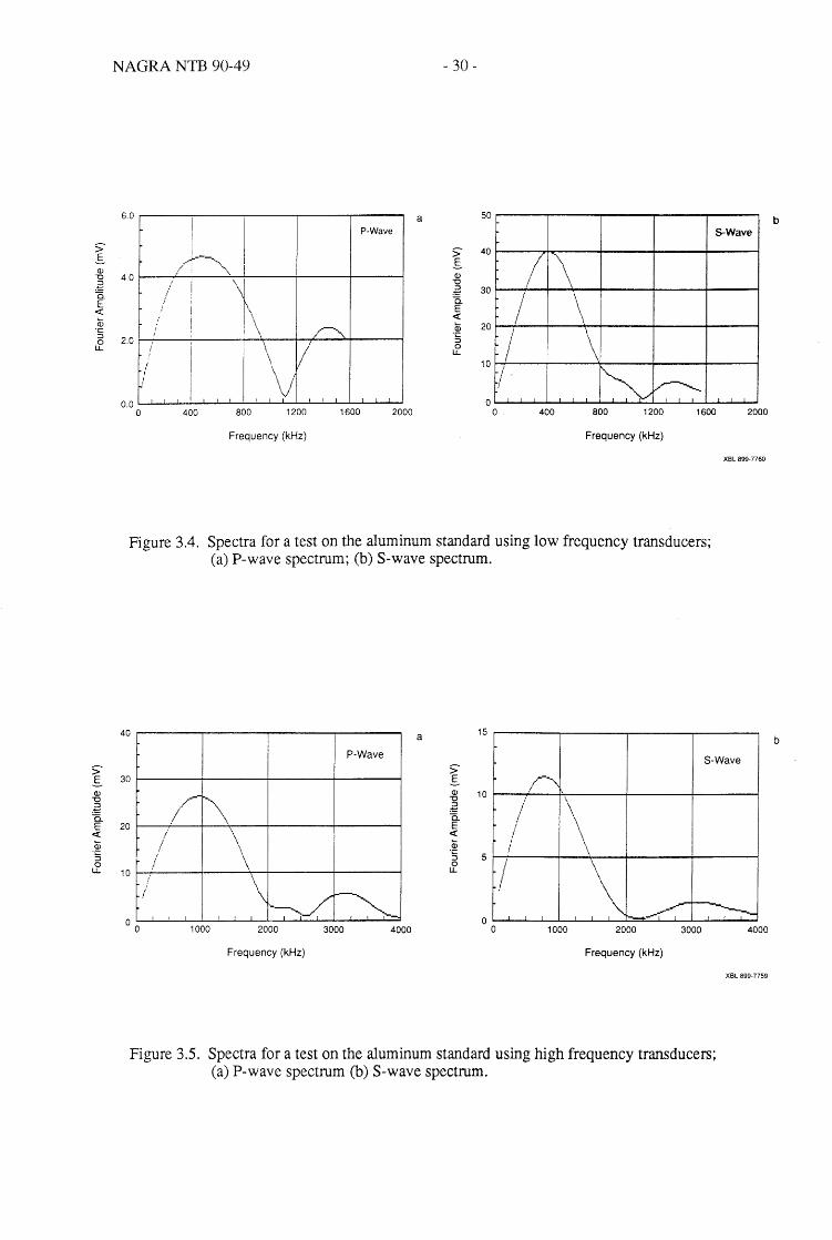
:;--S CIJ
" :~ C:i E
<t: Q) "§ 0 u..
:;-.s
CIJ
" .~ Ci E <t: Q) "§ 0 u..
NAGRA NTB 90-49 - 30-
6.0 i
a 50
I P-Wave S-Wave
i
4.0
2.0
... J-----._, /.... . .... \
/. i l\ I
I
" ! / . ..--. ........
, \; 1/ / I I
~'
0.0 I I
o 400 800 1200 1600
Frequency (kHz)
:;--S CIJ
" :~ C:i E <t: to "§ 0 u..
2000
40
30
20
10
o o
I /.
( \ / I \
\\
,~ .... ......--....... 400 800 1200 1600
Frequency (kHz)
Figure 3.4. Spectra for a test on the aluminum standard using low frequency transducers; (a) P-wave spectrum; (b) S-wave spectrum.
40 a 15
2000
XBL 899-7760
P-Wave S-Wave :;-
30
20
10
;/- -'''\ .I
I \ / /
! j
-S CIJ 10 "0
:E C:i E <t: to .~
5 ::J 0 u..
r-....., I ,
/ \ I \ .----....---/ ~- \ ,."r'" ---~
---""" o 0 1000 2000 3000 4000 o
o 1000 2000 3000
Frequency (kHz) Frequency (kHz)
Figure 3.5. Spectra for a test on the aluminum standard using high frequency transducers; (a) P-wave spectrum (b) S-wave spectrum.
4000
XBL 899-7759
b
b

NAGRA NTB 90-49 - 31 -
both the low frequency and the high frequency transducers. Data acquisition was perfonned with
a LeCroy 8013A mainframe with an installed TR8818 Transient Recorder system. The TR8818 is
a digitizer designed for high speed, long record waveform recording, which converts an analog
input signal into 8-bit digital words at sampling frequencies from 0.01-100 MHz. The TR8818
was used with Wavefonn-Catalyst, a multichannel digital oscilloscope software package
intended for use on mM personal computers. The Waveform-Catalyst program allows acquisi
tion, averaging, and analysis of waveforms and was used for all experiments.
The sampling frequency for tests using the low frequency transducers was 6.25 MHz, yield
ing a Nyquist frequency of3.125 MHz. When the high frequency transducers were used, the sam
pling frequency was 25 MHz, yielding a Nyquist frequency of 12.5 MHz. Typically 20
wavefonns were averaged at each stress level.
The apparatus shown schematically in Figure 3.7 was used for the Wood's metal injection
tests. The specimen was first dried, and then was placed in the pressure vessel. The main body of
the vessel was centered on the fracture, and the fracture was sealed off with Vi ton O-rings
retained by aluminum compression rings. The specimen was then placed in the load frame as pre
viously described, and a set of waveforms was sampled at a set of prescribed loads. The speci
men was then placed under an axial stress of 5.72 :MPa (60 kN axial load). Strip heaters were
placed around the body of the pressure vessel and the transducers, and the body of the vessel was
heated. The vessel was heated to a temperature of 120°C, and the transducers to 90°C to prevent
loss of the heat through the ends of the specimen. These conditions were maintained for at least
two hours to insure uniform heating of the specimen. At the time of injection, liquid Wood's
metal was pressurized to 2 :MPa, and injected into the fracture. Once flow was detected through
the valve on the opposite site of the vessel, both the injection and the outlet valve were closed.
The heaters were turned off, and the specimen was allowed to cool for 24 hours with the axial
pressure remaining at 5.72 :MPa. Waveforms were then taken as the load on the specimen was
cycled. The pressure vessel was installed on all specimens to be injected with Wood's metal, or
whose wavefonns were to be compared with those specimens to be injected with Wood's metal.
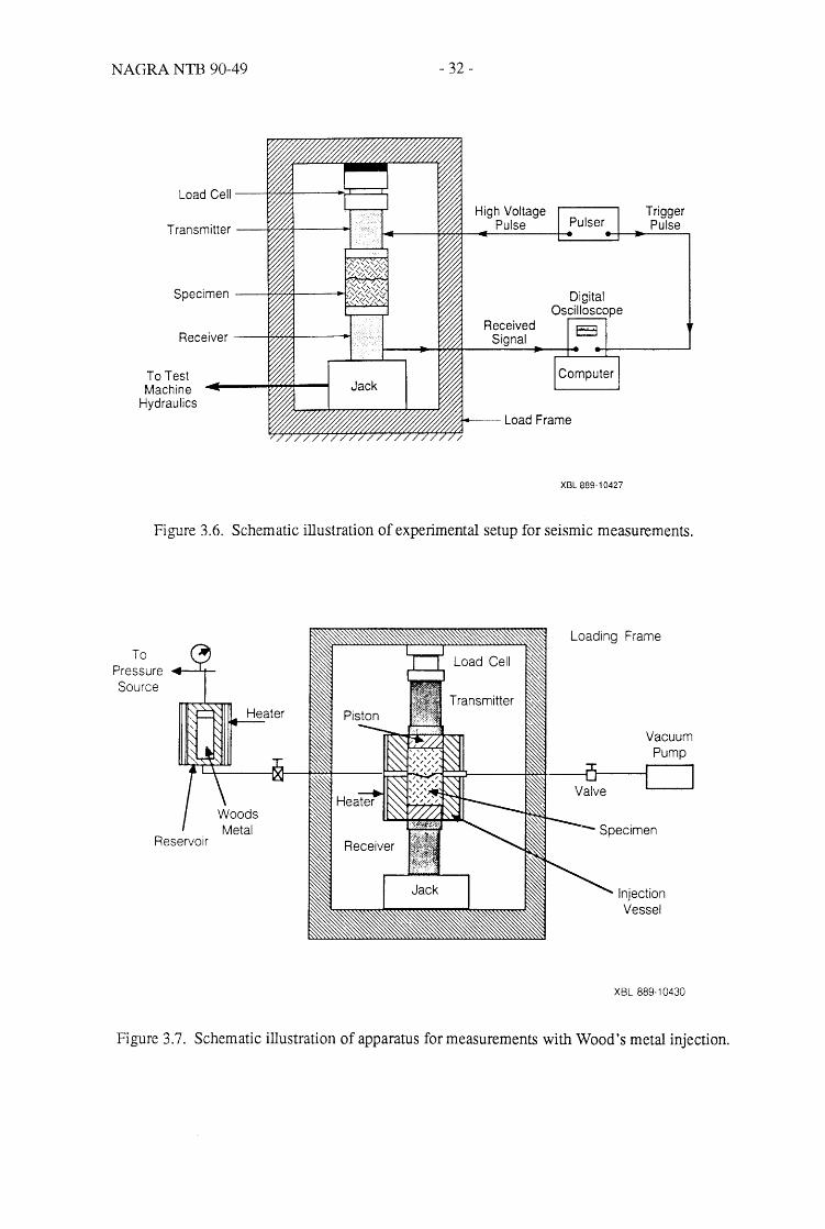
NAGRA NTB 90-49
Load Cell --+@4---~~==~
T ran smitter ----J;,yy;,t.;.4-----+I
Receiver --~"7'7I------+I
To Test Machine
Hydraulics
- 32-
High Voltage Pulse
Received Signal
Load Frame
XBL 889-10427
Trigger Pulse
Figure 3.6. Schematic illustration of experimental setup for seismic measurements.
To Pressure Source
Loading Frame
Injection Vessel
XBL 889-10430
Figure 3.7. Schematic illustration of apparatus for measurements with Wood's metal injection.

NAGRA NTB 90-49 - 33 -
A manifold similar to that illustrated in Figure 3.7 was placed around the specimen for tests
on the fractured specimens under saturated and dry conditions using the low frequency transduc
ers. All tests using the high frequency transducers were performed without a manifold, as shown
in Figure 3.6. In this case, to prevent fluid loss, the saturated samples were wrapped with foil.
3.5. Results of Laboratory Measurements
Examples of typical P- and S-wave waveforms for each of the various test conditions are
given in Figures 3.8 - 3.15. For each figure the first arrival pick and the corresponding travel time
through the sample is shown. Some of the waveforms are quite disturbed~ due to their low ampli
tudes, making it difficult to accurately determine the first arrival. This data was included, how
ever, because it demonstrated the effect on attenuation of changing conditions in the same rock. It
was important to show that changing some conditions resulted in increased attenuation even
though the poor data made the change difficult to quantify. For tests yielding disturbed
waveforms, picks were made by visually comparing all the waveforms from the test to identify
features which were consistent from one measurement to the next.
Velocities were calculated, and peak-to-peak amplitudes of the first arrivals were recorded
for waveforms taken during the experiments. These were plotted with respect to the axial load (1
leN corresponds to 9.5 x 10⁻² :MFa). Peak to peak amplitudes were used to describe attenuation
because they were the most readily obtainable data. Experience has shown that peak to peak
amplitudes show, to a first order, the same trends as more sophisticated spectral analysis. Also,
the quality of some of the data did not warrant the additional time needed to perform spectral
analysis. The amplitude of only the first arriving pulse was used to minimize effects of contami
nation of the waveform by reflections arising from the sample geometry. Dotted lines have been
added by hand to help delineate trends in the data.
The results are organized first (Section 3.5.1) to illustrate the effects of saturation on veloci
ties and amplitudes from tests using both the low and high frequency transducers. Amplitudes of
tests employing different transducers could not be compared. In Section 3.5.2 data is replotted in
order to illustrate the effects of a single fracture on velocities and amplitudes under the various

NAGRA NTB 90-49 - 34-
160 kN load, intact ambient specimen, low frequency, 3/23/88
: ...... """ .. " .. " .. """ .......... ''''' ... '''''' .. '''''' ...... '' ...... '' .. " .. " .. ''"""""'"'''S~W~'~e''''' b
, .. '. ,., ..... ,', ... ,., ... , ............ ' .... , ..... ,.,.,., ... ,
> ~ L_~ .,.".: ..... : .... ;F' .... ·· .. : .... .. o N
. , , . . , , ,
. .' , :." •••• "" ••• , •• "' •••••• " ••• : ••••••••••••••••••••• "'1"" ,
5 us/div 5 us/div
XBL 899-7768
Figure 3.8. Example waveforms for intact specimen, ambient conditions, low frequency transducers, 160 kN load level, total travel time of first arrival in Ils; (a) P-wave (b) S-wave.
160 kN load, intact specimen, saturated, low frequency, 9/16/88
" " .. " ",""" ... " .. ".""""" ....... ", .. " .. "."."."" .. " .. " .. " .. " ... """ ... "",, ... ,,.,, a P-Wave , , ..... ,' ...... , ",., ... " ... ,." .. , ..... .
. . , , , , , , ,
, . . .
~.\,~.\: ".',' '~~,~')\i ~ ~'" '!""IJ'f'" VyV\r ~,~,~ 24,56' \' , , :
, . , . , , ,
. ", .. ,., ,., , .. , .. , ... ',., ................ ,
5 us/div
>
~ E o T'"
.... , .. ,' .. ' ... ,."",, .... " .. ",.'.,,' ... " ...... , ... ' ... ',.·" .. '''·'''··· .. '''·'' .. '''''' .. ' .. · .... ''·S~Ij.j~~~'''·'' b " ,
"1""" , .' •• ,,"'0' .'
, , , , , . . . , , , , . . . . ... , ........... , .... " ... , .. " ...... ""'. ",.,.,.,.,.,., ... ,., .
5 us/div
XBL 899-7767
Figure 3.9. Example waveforms for intact specimen, saturated conditions, low frequency transducers, 160 kN load level, total travel time of first arrival in Ils; (a) P-wave (b) S-wave.

NAGRA NTB 90-49 - 35 -
160 kN load, fractured specimen, dry, low frequency, 9/28/88
" ................................. ·· .. ·· .. · .. ·· .. ·· .. · .. ·· .. · .. · .. ·p·~W~~~ .. ·· .. · a ................. " .. " ...... ".,', .. " .......... "., .. ,,', .... ······ .. ·' ...... ·"'·"'·· .. ··"··"·"'s·~~~~'~·'···' b
· . .... ,., ..... , .. · . .
I L'""}"i~l>'\~j· •• '"~'~W>.i • I . \:;oJ '\. . .... "V,. • :
: .................... , ............................ r. M% . . . . . .
. , . . .. '" , ..... " ... , ........ ""." ............ , .. , .., , ".
. . . . '.', ..... , ...... ".,., ... , .. ,.' .............. "., .. · , , · . . · . ,
.... """"" .. """""." ................. ,, ...... ,, ............. ,, .. ..
5 us/div 5 us/div
XBL 899-7766
Figure 3.10. Example wavefOITIls for fractured specimen, dry conditions, low frequency transducers, 160 kN load level, total travel time of first arrival in /-lS; (a) P-wave (b) S-wave.
160 kN load, new fractured specimen, saturated, low frequency, 9/2/88
P-Wave a S-Wave
b
~ tJj;J-{'vr~L:. rJ f6: : ..-_../: :: :: I
""""""<""""""'" ••• _,., II ".,.,.,.,., """ .,
: : : : 51.31: : .
5 us/div 5 us/div
XBL 899·7765
Figure 3.11. Example waveforms for fractured specimen, saturated conditions, low frequency transducers, 160 kN load level, total travel time of first arrival in /-lS; (a) P-wave (b) S-wave.

NAGRA NTB 90-49 - 36 -
160 kN load, intact specimen, dry, high frequency, 8/7/88
.................. " ............. , .... " ............... , .. " ......... , .... " ....... , ....... ,', ...... " ........ "" ....... : a P-Wave
.".,,, .. ,, .. ,,., ...... ,,,, .. ,,,,,,., .... ,,,.,,.,,,.,,,.,,,,, ... ,,,.,,,,,,,., .... ,, .. ,, ...... ,, ...... ,, .. ,, ...... ,, .. ,, ......... b
, , . - . .
~ ~_~O"~'~'"~."M"*"<r~ /\A 1\. ·jV~W·· •••••• ~. ~ ...... , ./,1 V V,/'",,~,:, ., ,:""",.""",'
29,76 ...:
>
~ E
.... , .. , .. ", .... , .. " .".,. .'0.,., ... ,.,_,.,.,.,., "t., •. ,', ••.•.•.•• ,',., .•. " •.•.•.• ,'
. . . .• I , ... ,., ... I,'.",.,., •. ", .•. "'"""": ..,.",.,." , .. ,.,.,.",.,."., .. ,.,.,-.", ... "".,.,.,.,., ,
5 us/div 10 us/div
XBL 899·7764
Figure 3.12. Example wavefonns for intact specimen, dry conditions, high frequency transducers, 160 kN load level, total travel time of first arrival in J.ls; (a) P-wave (b) S-wave.
160 kN load, intact specimen, saturated, high frequency, 9/21/88
a P-Wave S-Wave
I ~-'~!'·~\A l,l\~4~~\.t·· ..... ~if'1A.' ••••••••••••••.•••.• ' C\J . , ".' 1,,1 \I" .. /." ... \, :r"'''':''''''': t, " .. ,,"'"
~! • '.. I ' i 4I}}~\~~ftWM~
41.44 . . 23.52 : : : : : :,:.::::: V:,::::::':':::.:,:,:::::::':,:
.,.,.,.,.,., ." ........... " .... , ... , ..................... ,', ..
5 us/div 10 us/div
Figure 3.13. Example wavefonns for intact specimen, saturated conditions, high frequency transducers, 160 kN load level, total travel time of first arrival in J.ls; (a) P-wave (b) S-wave.
XBL 899· 7763
b

NAGRA NTB 90-49 - 37-
160 kN load, fractured specimen, dry, high frequency, 9/21/88
, ............ , .. " .......... " .................. ", ... " .. ,." .. ,', ..... , .. , .. ' ........ . a S-Wave
b P-Wave
>
~ E
~ I 1 ~ ",. ~,1,1! ;f\h .. ~YlV~V~" . ~ \IM"'*h~ I\,!rl}.l .•.•.•.•••..•
33.32 •• , , ••• , " • "I , ••• , ,. """
> ~ > E o N
10 us/div 10 us/div
XBL 899· 7762
Figure 3.14. Example WaVefOlTIlS for fractured specimen, dry conditions, high frequency transducers, 160 leN load level, total travel time of first arrival in Jls; (a) P-wave (b) S-wave.
160 kN load, fractured specimen, saturated, high frequency, 9/5/88
P-Wave a
5 us/div
S-Wave .,., """",' .... ",.,." "., """"""""""""""'"
~ , · ~<!t~~' f ~ \'~!Y\)l.~.... .•.••. .• .!\\: : . 42.84 .
• • • • • • • • • to, ••• , ••• ,.,. I , •••••••
10 us/div
XBL 899·7761
Figure 3.15. Example waveforms for fractured specimen, saturated conditions, high frequency transducers, 160 leN load level, total travel time of first arrival in /ls; (a) P-wave (b) S-wave.
b

NAGRA NTB 90-49 - 38 -
test conditions. Heterogeneity in the rock introduced ambiguity in the comparison of results
from fractured and intact specimens, so a test was perfonned in which one of the specimens was
injected with Wood's metal. Comparison of seismic attenuation before and after Wood's metal
injection are presented in Section 3.5.3.
3.5.1. Effects of Saturation
Velocity Data. P- and S-wave velocities at low frequency for intact specimen #3 under
ambient and saturated conditions are shown in Figures 3.16a and 3.16b, respectively. The veloci
ties increased with increasing load for both ambient and saturated conditions, reflecting the clo
sure of cracks in the matrix of the rock The effect is pronounced, particularly for ambient condi
tions, probably because the foliation of the sample is perpendicular to the direction of the load
ing.
Though the ambient condition specimen was not vacuum or oven dried, a difference in both
the P- and S-wave velocities for ambient and saturated conditions is apparent. This difference
between the ambient and saturated velocities is particularly pronounced for the P-wave. Under
saturated conditions the P-wave velocities under 40 k.N load was 5100 mis, approximately I5()()
mls higher than for dry conditions. At 150 kN load the difference is approximately 1000 m/s. The
saturated P-wave velocity appears to asymptote in the region of 5700 m/s. The ambient P-wave
velocity, beginning at 3000 m/s at 25 kN load, rises to 4500 mls at 150 leN load. At a load where
all cracks are fully closed, the velocities should asymptote towards the same value. The S-wave
velocities display the same behavior; velocities increase with increasing axial load for both
ambient and saturated conditions. Saturated S-wave velocities begin. at 24()() m/s at 10 kN,
increasing to 2700 mls at 150 leN, and asymptoting to approximately 2800 m/s. The ambient S
wave velocity begins at 2250 mls at 20 kN load, increasing to 2650 mls at 150 kN load.
The fractured specimen, specimen #2, exhibited similar behavior. Velocities increased with
increasing load, with the P-wave velocity behavior corresponding particularly well with the
behavior in the intact specimen. Figure 3.17a shows the velocities for the P-wave for two experi
ments with specimen #2 oven dried and saturated. The data is remarkably similar considering the

(j)
NAGRA NTB 90-49 - 39 -
Dry (ambient) vs. Saturated Low Frequency, Intact
6000-,------------------------, 2900.--------------,--------,
- .J---• --. (a) 2800- •
(b)
• E 5000-....--1---- ~ 2700- / _/6
E .// • -~ '0 o
Ci5
-.....g--""-
/ 0
.0'
..0/ ;;: 2600 - / ./ 0 /'./ 0
.g 2500 - • /' {" / /'
> 4000- ° /-H' - 7' 0--/ 0 g; ,.. /'
0..
-/
00// 0 /'
0/ 0
/
o 3/23/88 dry • 9/16/88 sat
3000-l---L1....bO"----.----,..----,_-----i
o 50 100 150 200
Load (kN)
C/) 2400- I 0 / • / 0
2300- B / B/O
o 3/23/88 dry • 9/16/88 sat
2200~-----r_1----,-,-----"----~ o 50 100 150 200
Load (kN) XCG 899·4682
Figure 3.16. Comparison of velocities for ambient and saturated conditions, intact specimens, low frequency transducers; (a) P-wave; (b) S-wave.
Dry vs. Saturated Low Frequency, Fractured
6000.....------------------- 3200..-----------------------
(a) (b) 3000 - J _ - - - -t- - - - ...
(fJ • ___ ~ - .- - • •
15000 •• I (j) 1 2800
~ ·0 o
->-."5 2600 o
Ci5 > 4000-
9-----0
° ~ 2400 C/)
012127/88 dry • 12115/88 sat. o 9/28/88 dry .912188 sat.
0..
-o 12127/88 dry • 12/15/88 sat. o 9/28/88 dry .9/2/88 sat.
3000~-,---.-,--r__.-,l,_-,_,_.l---r_I~
o 50 100 150 200 250
Load (kN) 50 100 150 200 250
Load (kN) XCG 899·4683
Figure 3.17. Comparison of velocities for dry and saturated conditions, fractured specimens, low frequency transducers; (a) P-wave; (b) S-wave.

NAGRA NTB 90-49 - 40-
length of time between tests and that the transducers were modified in the interval between
9/28/88 and 12/15/88. S-wave velocities were not as easily interpreted, in part due to the
difficulty of determining the first arrival of the wave in many cases. This may account for the
anomalous nature of the 12/15/88 saturated velocity data in Figure 3.17h. Except for this, Figure
3.17 shows that both p- and S-wave velocities were higher under saturated conditions.
The general trend shown by the results from velocity measurements using the low fre
quency transducers is that saturation has an effect on both P- and S-wave velocities, yielding
higher values for both types of wave, although the effect on the P-wave is the largest. The
difference diminishes with increasing axial stress. For P-waves this behavior can be ascribed to
the effects of microcracks on the modulus of the rock; the modulus would be expected to increase
with both saturation and or increased axial stress. For S-waves, increasing velocity would also
result from microcrack closure as axial stress increased. However, saturation, by conventional
models, should not affect the shear modulus. The results also show that the effect of the single
fracture on velocities for these specimens under either the intact or saturated conditions did not
dominate in this rock type.
P- and S-wave velocities for the intact specimen under dried and saturated conditions using
the high frequency transducers are plotted in Figures 3.18a and 3.18.b, respectively. The P-wave
velocities for the dry condition are considerably less than for the saturated condition. For dry
conditions, the velocities begin at 3500 mls at 50 kN and increase with load to 4700 mls at 150
kN, while for the saturated condition, values range from 4900 mls to 5600 mIs, respectively. For
the range of loads used in L~e test, velocities for the dry and saturated conditions asymptote to
5100 mls and 5800 mIs, respectively. S-wave velocities behave similarly; the dry velocities
beginning at 2250 mls at 20 leN load and increase to 2800 mls at 150 kN; the values for the
saturated condition 2650 mls to 3100 mIs, respectively. The saturated velocity asymptotes to
3200 mIs, and the dry velocity to about 3000 mls. These values are unifonnly higher than those
obtained using the low frequency transducers. It is also interesting to note that the difference
between day and saturated are larger for the high frequency S-waves than for low frequency S-

NAGRA NTB 90-49 - 41 -
waves, especially at higher loads.
Figures 3.19a and 3.19b are high frequency P- and S-wave velocities, respectively, for the
fractured specimen under dry and saturated conditions. Velocities for the dry fractured specimen
appear to be a linear function of load for both the P- and S-waves. Saturation results in a pro
nounced increase in both P- and S-wave velocities. P-wave velocities for the fractured specimen
under saturated conditions are similar to those for low frequencies (see Figure 3.16a), but S-wave
velocities are 400 m/s higher at 20 kN load, and 100 m/s higher at 150 kN load.
Results of tests using high frequency transducers were similar to those of the low frequency
transducer in that velocities under saturated conditions are typically higher than those for the
dried condition.
Amplitude Data. Peak-to-peak amplitude data for measurements made using low frequency
transducers are shown in Figures 3.20-3.21. Figures 3.20a,b and 3.2Ia,b compare amplitudes for
the fractured specimen in dry and saturated conditions. Figures 3.2Ga and 3.2Gb present data prior
to modifications on the low frequency transducers (Section 3.4) willIe Figures 3.21a and 3.21b
present data after modifications. The figures show that amplitudes increase as axial load
increases, which is a reflection of the influence of the microcracks. As the microcracks are closed
at higher stresses, less attenuation is expected. Figure 3.20a shows that saturating the specimen
resulted in increases in P-wave amplitudes of 2-4 times. Comparison with Figures 3.20a and
3.21a show that the P-wave data obtained at a later date exhibited the same trend but there was
less difference between amplitudes for dry and saturated conditions in the later tests.
The effect of saturation on S-wave amplitudes for the fractured specimen is shown in Fig
ures 3.20b and 3.21b. The behavior of the S-wave amplitudes is quite different from that of the
P-wave amplitudes. The S-wave amplitudes under dry conditions increase with axial stress much
more rapidly than those under saturated conditions. Thus, at low loads, the S-wave amplitudes
under dry conditions were equal or less than those under saturated conditions, but under high
loads they were much greater than the amplitudes under saturated conditions. Note the similarity
in the S-wave amplitude trends shown in Figures 3.2Gb and 3.21 b even though the tests were

c '(3 o
NAGRA NTB 90-49 - 42-
Dry VS. Saturated High Frequency, Intact
6000~----------------------------------, 3200 ~------------------------------,
- • ~-- ... ---• • •
(a) -3000-
Vi" -E 2800- '" >. a/ ''5 - .,. -/
.. .-e.- - - .. -,, __ -- e fIf//
(b)
/ /
/ o
~ 4000-CL
~ 2600- / ~ > /
CJ) - /+
- 08/7/88 dry .8/4/88 sat. • 9/21/88 sat.
3000 -4----------r-------r------.......--------; o 50 100 150 200
Load (kN)
2400- •
-0817/88 dry e 8/4/88 sat. • 9/21/88 sat.
2200 -1-------.......-,-----..---,------.,------1 o 50 1 00 1 50 200
Load (kN) XCG 899-4688
Figure 3.18. Comparison of velocities for dry and saturated conditions, intact specimens, high frequency transducers; (a) P-wave; (b) S-wave.
Dry VS. Saturated High Frequency, Fractured
6000~--------------------------~ 3200 -r-----------------------------., (a) (b)
- ---------- . - ,------. (j) --- -#--E 5000- I
_ 3000-(f)
• •
.?:'(3 o 03
-
/
cv --c
/
/ /0
/
E >. 13 2800- • o
/
/ .D
/0
/
...0/
/
> 4000 / 0/
0/ 03 >
CL / / 0
o 9/21/88 dry .9/5/88 sat.
3000 --+-----------,------------,,--------,-------1 o 50 100
Load (kN) 150 200
CJ) 2600-
-0/
/ /
o / 0 /
-1::J /
09/21/88 dry .9/5/88 sat.
2400-+------,..,..--------.-_____ ----,-____ ~ o 50 100
Load (kN) 150 200
XCG 899-4690
Figure 3.19. Comparison of velocities for dry and saturated conditions, fractured specimens, high frequency transducers; (a) P-wave (b) S-wave.

NAGRA NTB 90-49
120
-
- 43-
Dry VS. Saturated Low Frequency, Fractured
400 -----. (b)
:> 100-_.---- (a) :>
-S 300
o -S CD
"0
.~ Q. E CO CD > CO 3: 0..
:;;-E-Q) "0
:~ c. E (ij
Q)
> (ij
~ cL
-........ ....... •
80-/'
........ - .1/
60- . / /
- • 40-
.......... 0
- ....-20 -
0 .............. -n 09/28/88 dry
- .912188 sat.
0 I
0 50 100 150
Load (kN)
CD "0
~ -
Q. 200 E CO Q.) > CO 100 3:
ch
/
....... ....... o /'
/' /
/
.-0- .- .-
o
/ . ------. / _i_------.---: -t- - 09/28/88 dry
/ .912188 sat. o n 0
I
o 50 100 150
Load (kN) XCG 899·4686
Figure 3.20. Comparison of peak to peak amplitudes for dry and saturated conditions, fractured specimen, low frequency transducers; (a) P-wave (b) S-wave.
100
• - / /
80- / /
- / / •
60- • / ,/
,/ - .,/ ,/ ....-• .......g 40- ,/ ./ . ,/'/ . ./ - ./
./ / 0'" 20- ./ . ,/
/ -
0 I I I
0 50 100 1S0
Load (kN)
• /
0
....-....-....-./
Dry VS. Saturated Low Frequency, Fractured
600 (a)
:;-SOO E
"- -Q)
....- "0 400
.~ -0 g. 300-
(ij -
Q)
> 200-
(ij -o 12/27/88 dry ~ 100-
//0 (b) /
/ CV'
/--0 /
/ ,/
0'/ P
,/ ,/
/8 .. ----. ---. 4!.-......-• 12115188 sat rh - . o 12127/88 dry - t' --r- • • 12115/88 sat 0 I I I I I I I I I
200 2S0 0 SO 100 1S0 200 2S0
Load (kN) XCG 899-4684
Figure 3.21. Comparison of peak to peak amplitudes for dry and saturated conditions, fractured specimen, low frequency transducers after modifications; (a) P-wave (b) S-wave.

NAGRA NTB 90-49 - 44-
separated in time by a considerable amount and the transducers had also been rebuilt.
Peak to peak amplitude data for measurements made using high frequency transducers are
shown in Figure 3.22 and 3.23. Figures 3.22a and 3.22b compare p. and S-wave amplitudes for
the fractured specimen under dry and saturated conditions. The observed trends are very similar
to those obtained using the low frequency transducer. Figures 3.23a and 3.23b compare P- and
S·wave amplitudes for the intact specimen under dry and saturated conditions. Here, again it is
seen that the P- wave amplitudes obtained under saturated conditions are larger than those for the
dry conditions, and in both cases amplitudes increase roughly linearly with increasing load. For
S-waves, however, while the amplitudes of the dry test increase nearly linearly with load, the
amplitudes from the saturated test tend to asymptote toward a constant level, lower than that of
the dry test, at higher loads. These trends are very similar to those observed for the fractured sam
ple.
3.5.2. Comparison of the Fractured and Intact Samples
Both the velocity data and peak to peak amplitude data collected under the various test
conditions were replotted to compare results from fractured and intact specimens. This technique
had previously been used successfully (Pyrak-Nolte et al. 1990) to demonstrate the effect of a sin
gle fracture on wave propagation. Based on this previous work it was anticipated that velocities
in the fractured specimens would be slightly less than or nearly equal to those in intact speci
mens. Significant differences between amplitudes, however, were expected. In particular, the
previous work indicated that amplitudes of both p- and S-waves in the fractured specimens
should be less than those in the intact specimens. This difference should diminish as load is
increased for both P- and S-waves and, for P-waves, the difference should also diminish under
saturated conditions.
Results from comparisons of data for fractured and intact specimens of the FRI core were
ambiguous. For several tests there was very little difference between velocities for the fractured
and intact specimens, while, for other tests the velocity in the intact specimen was higher. Simi
larly, the amplitude of waves transmitted through the fractured sample were actually larger than

NAGRA NTB 90-49
120 - ./ •
- 45 -
Dry VS. Saturated High Frequency, Fractured
100
(a) - (b)
::> 100- • ./
-S /'
./ ::> E- 80- o /'
/' ,/
/' 0
0) "'0
.~ Q. E C'C! 0)
> C'C! ~
cL
/' /'
80 /' /'
/' • /'
60 /' • 9/5/88 sat.
~ o 9/21/88 dry
0) "'0
.~ 60
Q. E ctl 40 -
,/ 0 o ,/ /'
~ ,/
0,/ ,/
.,/ 40
I' 20 0 0 m 0
0) ->
ctl ~ 20 -
ch -
,/
0'/ 0
#' -- - - - - - - - - -. 9/5/88 sat. ,/ /' 09/21/88 dry
• 0 I I
0 50 100 150 200 0
0 I
50 I
100 I
150 200
Load (kN) Load (kN) XCG 899·4687
Figure 3.22. Comparison of peak to peak amplitudes for dry and saturated conditions, fractured specimen, high frequency transducers; (a) P-wave (b) S-wave.
Dry VS. Saturated High Frequency, Intact
30~----------------------~.------~
(a) 80~----------------------~D~----~
(b) ---. ,,- • " .. ./ ......
..gs 20 ././ •
. ~ • ././. .0" Q. /'./, // E /' ~./ ctl /. /-tJ 0) 10- I 9-/ > ./-"tl
~ .. ' ~ 0..
, -, /' D)Y 0
o 8n/88 dry • 8/4/88 sat. • 9/21/88 sat.
o 8n188 dry • 8/4/88 sat. • 9/21/88 sat.
O+-------~------~------~------~ I
o 50 150 200 o 50 100 150 200 100
Load (kN) Load (kN) XCG 899-4689
Figure 3.23. Comparison of peak to peak amplitudes for dry and saturated conditions, intact specimen, high frequency transducers; (a) P-wave (b) S-wave.
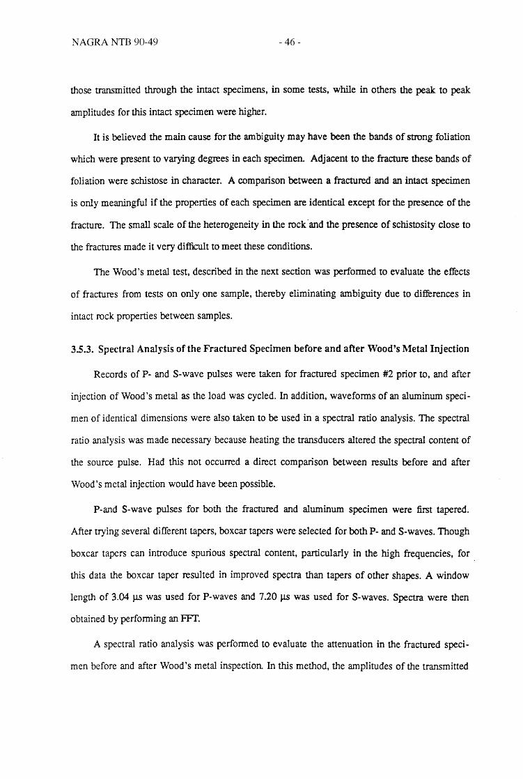
NAGRA NTB 90-49 - 46-
those transmitted through the intact specimens, in some tests, while in others the peak to peak
amplitudes for this intact specimen were higher.
It is believed the main cause for the ambiguity may have been the bands of strong foliation
which were present to varying degrees in each specimen. Adjacent to the fracture these bands of
foliation were schistose in character. A comparison between a fractured and an intact specimen
is only meaningful if the properties of each specimen are identical except for the presence of the
fracture. The small scale of the heterogeneity in the rock "and the presence of schistosity close to
the fractures made it very difficult to meet these conditions.
The Wood's metal test, described in the next section was performed to evaluate the effects
of fractures from tests on only one sample, thereby eliminating ambiguity due to differences in
intact rock properties between samples.
3.5.3. Spectral Analysis of the Fractured Specimen before and after Wood's Metal Injection
Records of p. and S-wave pulses were taken for fractured specimen #2 prior to, and after
injection of Wood's metal as the load was cycled. In addition, waveforms of an aluminum speci
men of identical dimensions were also taken to be used in a spectral ratio analysis. The spectral
ratio analysis was made necessary because heating the transducers altered the spectral content of
the source pulse. Had this not occurred a direct comparison between results before and after
Wood's metal injection would have been possible.
P-and S-wave pulses for both the fractured and aluminum specimen were first tapered.
After trying several different tapers, boxcar tapers were selected for both p. and S-waves. Though
boxcar tapers can introduce spurious spectral content, particularly in the high frequencies, for
this data the boxcar taper resulted in improved spectra than tapers of other shapes. A window
length of 3.04 J.1S was used for P-waves and 7.20 J.1S was used for S-waves. Spectra were then
obtained by performing an FFf.
A spectral ratio analysis was performed to evaluate the attenuation in the fractured speci
men before and after Wood's metal inspection. In this method, the amplitudes of the transmitted

NAGRA NTB 90-49 - 47-
waves are assumed to take the fonn
(3.1)
where x is the length of the wave path, G(x) is a factor incorporating the effucts of the geometry
of the specimen (such as spreading of the wave and reflections), f is the frequency of interest, k is
the wavenumber, t is the time and aCt) is the attenuation coefficient. If the same test is run on a
second specimen (which could be a reference aluminum specimen), the ratio of amplitudes from
the two measurements is given by:
Ai Gi -(y,. -'tJ)fx -=-e 1 J
A· G· J J
(3.2)
in which it is assumed that a(t) = yr. If the natural logarithm of both sides of (3.2) is taken, the
resulting equation is
(3.3)
where y = ...1L and c is the phase velocity of the medium. For a high Q reference material Yi is Qc
very small, and can, to the first order, be neglected. In addition for specimens of identical
geometry, G(x) are identical, and their ratio is unity. Under such assumptions Equation (3.3) can
be used to determine the attenuation coefficient of the material of unknown properties, since .l Q
is the slope of the graph of the log amplitude ratio vs. frequency. In the special case where a is
not a function of frequency, the slope of the line is constant.
Plots comparing spectral ratios at different axial load levels before and after Wood's metal
injection are shown in Figures 3.24a,b,c and 3.25a,b,c, for P- and S-waves, respectively. The load .
levels refer to the load applied to the rock.. The aluminum reference spectrum for the plot labeled
120 kN consisted of the average of two spectra obtained at loads of 80 leN and 160 leN. For the
plot labeled 320 leN, the aluminum reference spectrum was obtained at 300 leN load.
The first characteristic of these curves to be noted is that, typically, for the results before
injection, there is a discontinuity in slope, in the range of about 450 kHz to 650 kHz for P-waves,

NAGRA NTB 90-49
N
~ $ Z ..J
N ~ $
Z ...l
6
5
4
3
2 0
4
3
2
0
-1 0
- 48 -
Spectral Ratios Before, After Injection
100
100
200 300 400 500 600 Frequency (KHz)
~ Pbef.2401eN -..-- P aflo 240 leN
200 300 400 500 600 Frequency (KHz)
700
700
4~----------------------------------~~~
3
2
100 200 300 400 500 600 700 Frequency (KHz)
XBL 907-2571
Figure 3.24. Comparison of log spectral ratios forP-waves before and after Wood's metal injection at axial loads of (a) 120 kN, (b) 240 kN, and (c) 320 kN.

NAGRA NTB 90-49
N ~ ~ Z ..l
N ~ ... ~
Z ..J
3
2
0
·1 0
3
2
0
·1 0
- 49-
Spectral Ratios Before, After Injection
100
--e-- S bef.l20 leN un!.
~ S aft 120 leN un!.
200 300 400 Frequency (KHz)
--e- S bet. 240 kN --+- S aft. 240 kN
100 200 300 Frequency (KHz)
400
3~------------------------------------~
2
o 50 100 150 200 250 300 350 400 450 Frequency (KHz)
XBL 907-2572
Figure 3.25. Comparison of log spectral ratios for S-waves before and after Wood's metal injection at axial loads of (a) 120 kN, (b) 240 kN, and (c) 320 kN.

NAGRA NTB 90-49 - 50-
and about 250 kHz to 350 kHz for S-waves. The frequency content of the first arrival is
represented by the region to the left of this slope change; to the right of the change there is very
little energy in the spectrum, so values of spectral ratio are not considered to be physically mean
ingful.
The second general characteristic is that the curves are non-linear. This means that the Q of
the rock, represented by the inverse of the slope of the curves, is a function of frequency. Com
parison of curves before and after Wood's metal injection at any of the loads shows that slope of
the curves is less after Wood's metal injection, corresponding to less attenuation. The effect is
particularly pronounced in the range of 450 kHz to 650 kHz for P-waves and 250 kHz to 350 kHz
for S-waves. While there was little energy in these frequency ranges before injection, there was
substantial energy present after Wood's metal injection. This means that the transmission of the
high frequencies was improved more by the presence of the Wood's metal than transmission of
the low frequencies. The negative slope of the spectral ratio curve over the range of 0-400 kHz
for P-waves at 320 kN after injection (Figure 3.24c) indicates the reverse trend of more attenua
tion at higher frequencies. This results remains unexplained.
The advantage of comparing results before and after Wood's metal injection as opposed to
comparing results from intact and fractured samples is that ambiguities due to compositional and
textural differences between samples are precluded. Thus the observed differences between
results before and after injection represent the effect of the voids, in and adjacent to the fracture,
on wave propagation. (The seismic impedance of Wood's metal is similar to that of granite).
Since the Wood's metal was injected into the fracture plane, if the rock adjacent to the fracture
were impermeable the differences in measurements before and after injection would be due only
to the void space in the fracture. After disassembly it was noted, however that Wood's metal had
intruded into the shistose layers adjacent to the fracture, and it is believed that the observed
behavior was primarily due to the effects of this intrusion.
The intrusion provides further evidence to support the hypothesis that water intrusion into
these same layers resulted in the higher velocities and larger than expected P-wave amplitudes in

NAGRA NTB 90-49 - 51 -
the saturated fracture tests. For P-waves the effect of either Wood's metal or water in the voids
would be to stiffen the rock.
3.6. Summary and Discussion
Compressional and shear wave velocities and amplitudes were measured as a function of
axial stress on an intact specimen and a specimen containing a single natural fracture. Measure
ments were perfonned on both specimens under dry and saturated conditions using two sets of
transducers of different frequencies. Measurements were also made before and after Wood's
metal was injected into the fracture.
Results showed that saturation had a dominant affect on velocities and amplitudes. For P
waves a pronounced increase in both velocity and amplitude resulted from saturating either the
intact or fractured specimen. An increase in P-wave amplitudes in response to saturation is con
trary to what is commonly observed in porous rocks at low saturation «90%). It is, however,
consistent, with measurements made on single fractures (Pyrak-Nolte, 1990). For S-waves the
effect of saturation was more complicated. S-wave velocities for the saturated intact and frac
tured specimens increased relative to the dry condition. S-wave amplitudes, however, at the high
axial loads, were higher for the dry condition than the saturated condition. Understanding the S
wave behavior should be addressed in further worle Of particular interest would be the effect of
the foliation (anisotropy) on S-wave velocities and attenuation.
Results of comparing velocities and amplitude for fractured and intact specimens were
ambiguous due, probably, to the foliation in the rock, which changed over short distances. To
eliminate the effects of sample to sample variations in foliation seismic measurements were per
formed on a fractured specimen before and after Wood's metal had been injected into the frac
ture. Results showed that the transmitted wave was less attenuated after the Wood's metal was
injected. Inspection of the specimen showed that Wood's metal not only filled the void space in
the fracture but also invaded the shistose layers adjacent to the fracture. The structure at a
microscale produced by the shistosity of the rock is, in many ways, analogous to the macroscopic
structure produced by fractures. Therefore it seems reasonable that the fracture stifihess theory

NAGRA NTB 90-49 - 52-
may be applicable to describing effects of the shistosity on both P- and S-wave behavior. In this
respect, work is currently underway to apply the theory to describing the effects of thin liquid
layers in fractures on S-wave transmissions.

NAGRA NTB 90-49 - 53 -
4.0. SEISMIC IMAGING EXPERIMENTS
4.1. Introduction
Borehole seismic methods offer promise on a variety of scales for characterizing the
significant mechanical and hydrologic features in an underground waste repository. As applied
on a repository-wide scale, the most likely borehole seismic method would be multi-offset/multi
source Vertical Seismic Profiling (VSP). On a smaller scale, the crosshole and VSP techniques
would be used for detailed characterization of the rock surrounding the mine working, canister
areas, and for "looking ahead" of the tunneling activities. By performing a tomographic
analysis of the VSP and crosshole data from multiple offsets and azimuths, it may also be possi
ble to map the fracture structure in greater detail than with conventional techniques. This data
could then be used in hydrologic or geomechanical models of fracture networks to study the
behavior of the rock mass. Before these methods can be applied in a routine fashion, many fun
damental questions remain regarding the propagation of seismic energy in fractured anisotropic
rock which must be addressed. This project was designed to address several of these issues by
perfomling controlled seismic, geomechanical, and hydrologic experiments in a well calibrated
environment.
The goal of the seismic experiments was to identify the factors that control the propagation
of seismic energy in a fractured anisotropic rock. When these factors are identi fied, it will be
easier to extrapolate fracture characteristics observable at the borehole walls and underground
workings to the entire repository block, thus providing a more complete set of data to character
ize the overall hydrologic and geologic parameters.
Three experiments were performed in the FRI site, one each in the summers of 1987, 1988,
and 1989. Presented here are the results of the 1987 and 1988 field studies in saturated condi
tions. The 1989 investigations repeated some of the previous measurements after air had been
injected into the fracture. These results are not reported here.
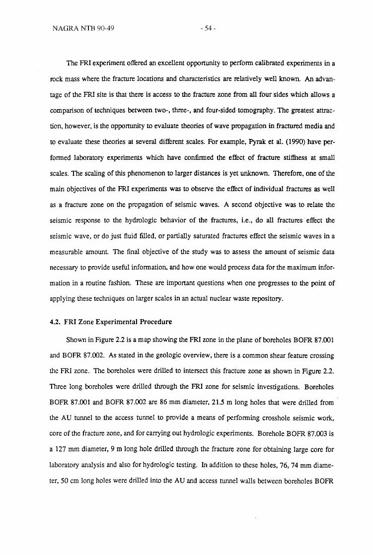
NAGRA NTB 90-49 - 54-
The FRI experiment offered an excellent opportunity to perfonn calibrated experiments in a
rock mass where the fracture locations and characteristics are relatively well known. An advan
tage of the FRI site is that there is access to the fracture zone from all four sides which allows a
comparison of techniques between two-, three-, and four-sided tomography. The greatest attrac
tion, however, is the opportunity to evaluate theories of wave propagation in fractured media and
to evaluate these theories at several different scales. For example, Pyrak et al. (1990) have per
formed laboratory experiments which have confirmed the effect of fracture stifihess at small
scales. The scaling of this phenomenon to larger distances is yet unknown. Therefore, one of the
main objectives of the FRI experiments was to observe the effect of individual fractures as well
as a fracture zone on the propagation of seismic waves. A second objective was to relate the
seismic response to the hydrologic behavior of the fractures, i.e., do all fractures effect the
seismic wave, or do just fluid filled, or partially saturated fractures effect the seismic waves in a
measurable amount. The final objective of the study was to assess the amount of seismic data
necessary to provide useful information, and how one would process data for the maximum infor
mation in a routine fashion. These are important questions when one progresses to the point of
applying these techniques on larger scales in an actual nuclear waste repository.
4.2. FRI Zone Experimental Procedure
Shown in Figure 2.2 is a map showing the FRI zone in the plane of boreholes BOFR 87.001
and BOFR 87.002. As stated in the geologic overview, there is a common shear feature crossing
the FRI zone. The boreholes were drilled to intersect this fracture zone as shown in Figure 2.2.
Three long boreholes were drilled through the FRI zone for seismic investigations. Boreholes
BOFR 87.001 and BOFR 87.002 are 86 mm diameter, 21.5 m long holes that were drilled from
the AU tunnel to the access tunnel to provide a means of performing crosshole seismic work,
core of the fracture zone, and for carrying out hydrologic experiments. Borehole BOFR 87.003 is
a 127 mm diameter, 9 m long hole drilled through the fracture zone for obtaining large core for
laboratory analysis and also for hydrologic testing. In addition to these holes, 76, 74 mm diame
ter, 50 cm long holes were drilled into the AU and access tunnel walls between boreholes BOFR
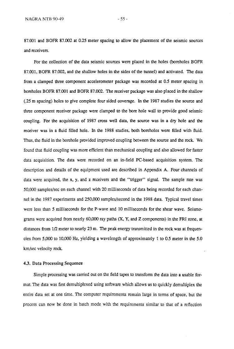
NAGRA NTB 90-49 - 55 -
87.001 and BOFR 87.002 at 0.25 meter spacing to allow the placement of the seisnllc sources
and receivers.
For the collection of the data seismic sources were placed in the holes (boreholes BOFR
87.0C)l, BOFR 87.002, and the shallow holes in the sides of the tunnel) and activated. The data
from a clamped three component accelerometer package was recorded at 0.5 meter spacing in
boreholes BOFR 87.001 and BOFR 87.002. The receiver package was also placed in the shallow
(.25 m spacing) holes to give complete four sided coverage. In the 1987 studies the source and
three component receiver package were clamped to the bore hole wall to provide good seismic
coupling. For the acquisition of 1987 cross well data, the source was in a dry hole and the
receiver was in a fluid filled hole. In the 1988 studies, both boreholes were filled with fluid.
Thus. the fluid in the borehole provided improved coupling between the source and the rock. We
found that fluid coupling was more efficient than mechanical coupling and also allowed for faster
data acquisition. The data were recorded on an in-field PC-based acquisition system. The
description and details of the equipment used are described in Appendix A. Four channels of
data were acquired, the x, y, and z receivers and the "trigger" signal. The sample rate was
50,000 samples/sec on each channel with 20 milliseconds of data being recorded for each chan
nel in the 1987 experiments and 250,000 samples/second in the 1988 data. Typical travel times
were less than 5 milliseconds for the P-wave and 10 milliseconds for the shear wave. Seismo
grams were acquired from nearly 60,000 ray paths (X, Y, and Z components) in the FRI zone, at
distances from 1/2 meter to nearly 23 m. The peak energy transmitted in the rock was at frequen
cies from 5,000 to 10,000 Hz, yielding a wavelength of approximately 1 to 0.5 meter in the 5.0
km/sec velocity rock.
4.3. Data Processing Sequence
Simple processing was carried out on the field tapes to transfonn the data into a usable for
mat. The data was first demultiplexed using software which allows us to quickly demultiplex the
entire data set at one time. The computer requirements remain large in tenns of space, but the
process can now be done in batch mode with the requirements similar to that of a reflection

NAGRA NTB 90-49 - 56 -
survey. The data are formatted such that the three components of each sweep of a stationary
source position are put into a file. Therefore, the number of files is equal to the number of sweeps,
or stationary source locations.
During acquisition, multiple signals were sometimes produced with the same source
receiver pairs in order to stack the data for improved signal qUality. After the data were demulti
plexed, the traces were stacked so that a single trace exists for each component of each source
recei ver pair.
43.1. Picking the Travel Times
The travel times were picked manually using an interactive picking routine developed at
LBL. The times were picked on the radial component (component 3), which is in the direction of
strongest P-wave motion. This was confirmed by rotating the data into the P-, SV - and SH
directions. Due to field equipment modifications the data quality was improved from 1987 to
1988. The source electronics used in 1988 was improved in power and rise time from the 1987
electronics so that the signal to noise ratio improved at higher frequencies. The repeatability of
this system resulted in more accurate travel time picks from the more consistent waveforms. This
can be seen by comparing Figures 4.1 (1987) and 4.2 (1988), a sample crosshole sweep from the
two data sets. The travel time picks are marked on each of the traces.
After the travel times have been picked, they were initially checked by plotting a time
distance curve (Figure 4.3a), a velocity-distance curve (Figure 4.3b) and a velocity vs. incidence
angle curve (Figure 4.3c). Any large variation from the general trend would indicate picking
errors or acquisition problems. Figures 4.4a through 4.4c show the corresponding 1988 plots,
respectively. As can be seen, the bulk of the 1988 travel time values (Figure 4.4) form a tighter
line than the 1987 values (Figure 4.4). The 1988 values which deviate from the tight line are
those which travel from the middle of BOFR 87.001 to the access tunnel, almost to BOFR
87.002. These values will be discussed later in the context of the interpretation. Compared to the
1988 data, the bulk of the 1987 travel time picks form a broader line of values indicating a
greater deviation in times. This is primarily due to the relatively large deviation in the picking of

NAGRA NTB 90-49 - 57 -
06105 COMP 3 31 37 ~7
31 497
.15 447
Jol 52"1
lJ 672
J:I '736
31 921
1O 12-4;
:II 1214
:II l1li2
27 lZ:>J
:II 15~
25 1333
c: 24 1080
~ II 1251!
IX! 22 1095 ::I 21 171e :::> :z: 20 1715
~ " 765 t) ,. bl4
~ 17 171<4
f-' ,. 1707
15 1'71i
1_
13 17Z5
12 610
11 1714
!O 1= 1667
1719
171C
l716
170e
16<Y.1
1303
615
702
I.DO 1.40 '''' 2.20 2.10 3.00 3.40 3.10 4.20 '.10 !..DO
TIME (WSECS)
DL '07-2524
Figure 4.1. Typical example of the crosshole 1987 P-wave data acquired at the FRI zone.
c: ~ IX! :s :::> :z: ~ t)
~ f-'
40 31 31 37 31 l!5 30 lJ 32 31
1O 2t
• 27 2t 25 24 II 22 21 20
" " 17
" 15 14
13 12 II
10 I
83105ES COMP 3
)~~~ !v-~ )J, '_V~-./'...J'-
'n Y/Y ~~ A~ .!hi
VN . v
'1'-'1. .~
7~,'A .~
~W'~'f ,-;:-r' ....,
:l\"IJ.".~ "',.... A
'iNJ'A'A -" VA :~ \'/.·fI'.II", "-
,~V;V-'V-·.V,V, J\ ""V"
~
'Y~\~~----7f~ .j.
" " y~, fWA "-rf'( II
jV/,\ i'I ~
~~v )J
r"~ , !':~
;y ~ v
lvr~ ~::.
v:~ \~J(;y . L I\, v
J71 35~
J36 373 489 520 bOO
662 671 588
520 ~5
526 623 bb6 606 74B
604 74J 851 746 1105
840 6Q.4
591 7.1 723
1022 729 8:le
BIB 8gB
631 615
617 519 312 452 355
I.DO 1.40 ,.., 2.20 2.10 3.00 3.40 J.8Cl ',20 ',10 !..DO
TIME (WSECS)
DL '07-2525
Figure 4.2. Typical example of the crosshole 1988 P-wave data acquired at the FRI zone. Shown on both figures are the picked arrival times.

W ~ F !rl ~ 1=
NAGRA NTB 90-49 - 58 -
a GRIMSEL 1987 b GRIMSEL 1987
'.0 '.10
•. 8 .... •. 0
I.'
•. U
'.11
+ .... + •
+~ .. ; + ,,'''f + -t..2t
+~* 1.0 I~
>-t: 2.8
U '.10 9
W >
2.0 .... t .• •. 12
1.0 . ... 0.1 •. M
0.0 -I-----,----.---.,-----r"---r---,...----,---..,.---,...--~ •.• 0 0.0 1,0 10,0 12,1 11.0 17.1 20.0 22.' 26.0 0.0 U 1.0 7.1 10,0 12.1 11.0 17.1 20.0 22.1 26,0
DISTANCE DISTANCE
XBL 907-2526 XBL 907-2527
>-
~ >
C
'.10
.... •. U
•. ,. 1.2.
'.10
.... •. 12
....
GRIMSEL 1987
+ +
... + + + t
++ +
+ +
+ + +
++
•.• 0 -l---,...-=---,-i-......!....,--~-,----.---.;--4"_____=:..,__i._.,--_ ___I -10.0 ·n,o -M.O -31,0 ·11.0 0.0 tl,O 31.0 ".0 n.o .0.0
INCIDENCE ANGLE
XBL 907-2528
Figure 4.3. (a) 1987 travel time versus distance data; (b) 1987 velocity versus distance data; and (c) 1987 velocity versus incidence angles. The dashed and solid lines are the least square fit of the data for the 1988 and 1987 data respectively, compare to Figure 4.4 for 1988 data.

~ ~
Ed ~ t=
NAGRA NTB 90-49 - 59-
a GRIMSEL 1988
1.0
•. 8
•. 0
1.8
1.0
~ u 9
W >
1.0
U
1.0
0.5
b
1.10
.... '.12
•. " .~
1.10
.... 4.11
4.11
4.84
+ +
++
GRIMSEL 1988
+ + .. +
20.0 21.1 •. 40+-----,,------r--...,.----,---,---,.-----r---,---,.----J
0.0 5.0 10.0 12.1 11.0 17.1 0.0 1.1 1.0 7.5 10.0 12.5 18.0 17.8 DISTANCE DISTANCE
XBL 907-2529
c GRIMSEL 1988
1.10
1.11
1.12
1.31
5.24
>-t::
9 1.10
w + > ++
4." + ... ++++ + + ++ ... .; +
+ + + + * 4.12 ;.
r- +
+~+ + + + +
4."
+
4 .• 0.+'-0.-0 -.n--'-.0--'-II<I'.0--.-3".-0 --.,"",.-0---'0-.0--""-' .O--'''''~-.O---'~-.o--n''-' .0----1J.
4.84 +
INCIDENCE ANGLE
XBL 907-2531
Figure 4.4. (a) 1988 travel time versus distance data; (b) 1988 velocity versus distance data; and (c) 1988 velocity versus incidence angles. The dashed line is the least square fit of the data for the 1987 data, the solid line is the fit for the 1988 data, compare to Figure 4.3 for 1987 data.
20.0 21.1
XBL 907-2530
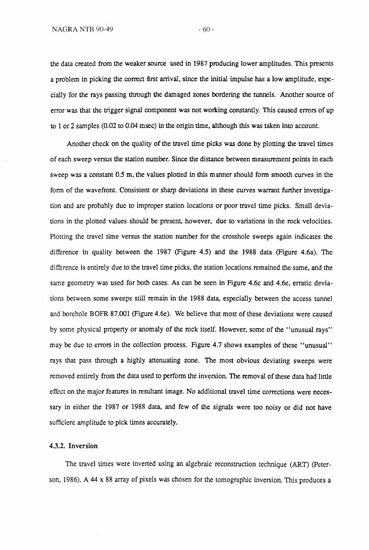
NAGRA NTB 90-49 - 60-
the data created from the weaker source used in 1987 producing lower amplitudes. This presents
a problem in picking the correct first arrival, since the initial impulse has a low amplitude, espe
cially for the rays passing through the damaged zones bordering the tunnels. Another source of
error was that the trigger signal component was not working constantly. This caused errors of up
to 1 or 2 samples (0.02 to 0.04 msec) in the origin time, although this was taken into account.
Another check on the quality of the travel time picks was done by plotting the travel times
of each sweep versus the station number. Since the distance between measurement points in each
sweep was a constant 0.5 m, the values plotted in this manner should fonn smooth curves in the
fonn of the wavefront. Consistent or sharp deviations in these curves warrant further investiga
tion and are probably due to improper station locations or poor travel time picks. Small devia
tions in the plotted values should be present, however, due to variations in the rock velocities.
Plotting the travel time versus the station number for the crosshole sweeps again indicates the
difference in quality between the 1987 (Figure 4.5) and the 1988 data (Figure 4.6a). The
difference is entirely due to the travel time picks, the station locations remained the same, and the
same geometry was used for both cases. As can be seen in Figure 4.6c and 4.6e, erratic devia
tions between some sweeps still remain in the 1988 data, especially between the access tunnel
and borehole BOFR 87.001 (Figure 4.6e). We believe that most of these deviations were caused
by some physical property or anomaly of the rock itself. However, some of the "unusual rays"
may be due to errors in the collection process. Figure 4.7 shows examples of these "unusual"
rays that pass through a highly attenuating zone. The most obvious deviating sweeps were
removed entirely from the data used to perfonn the inversion. The removal of these data had little
effect on the major features in resultant image. No additional travel time corrections were neces
sary in either the 1987 or 1988 data, and few of the signals were too noisy or did not have
sufficient amplitude to pick times accurately.
4.3.2. Inversion
The travel times were inverted using an algebraic reconstruction technique (ARn (peter
son, 1986). A 44 x 88 array of pixels was chosen for the tomographic inversion. This produces a

NAGRA NTB 90-49
0 ~ ~
~ 1= ..J
~ ~
- 61 -
CROSS BOREHOLE 1987
4.1
4.2
S.I
S.I
S.3
S.O
2.7
2.4
2.1
u
u+---r---.,---.,---,.------,-o----,---,----,...----.-----l m m m ~ ~ ~ ~ ~ ~ ~ ~
STATION NUMBER
XBL 907-2532
Figure 4.5. The travel time versus station number for the 1987 crosshole data, compare to Figure 4.6a.
0 w I/)
~ w :E 1=
I
CROSS BOREHOLE 1988
4.00
S.71
S.IO
1.21
1.00
2.71
2.10
2.21
2.00
1.71
1.1O-!--..,..--.,..---.,....--,.-----,..------.---,-----,.----,----1 u II " ~ m m ~ w ~ ~ ~
STATION NUMBER
XBL 907-2533
Figure 4.6a. Travel time versus station number from the 1988 crosshole paths for rays actually used in the final inversion.
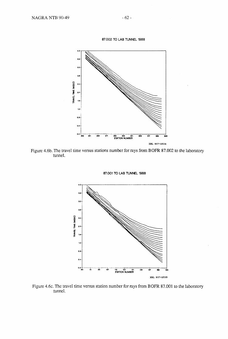
NAGRA NTB 90-49
E II)
~ w :E 1= -I W
~ 1=
- 62-
87.002 TO LAB TUNNEL 1988
•. 0
J.I
U
2..
2 .•
2.0
1.1
1.2
0.1
0 .•
O.O+---.----r----.---,.-----.-----.---,-----,---"T"----l 2U 211 211 zn 21& 213 301 JOt 117 aa IU
STAnON NUMBER
XBL 907-2534
Figure 4.6b. The travel time versus stations number for rays from BOFR 87.002 to the laboratory tunnel.
0 ~ ~ w :E 1= -I W
~ e:
87.001 TO LAB TUNNEL 1988
•. 0
3.1
U
2..
2 .•
2.0
"j 1.2
0.1
0 .•
0.0+---r----,...--,.-----,-----r---,-----,----.----.----1 13 II .. 107 115 123 131 131 M7 111 In
STAnON NUMBER
XBL 907-2535
Figure 4.6c. The travel time versus station number for rays from BOFR 87.001 to the laboratory tunnel.

NAGRA NTB 90-49
0 UJ
'" ~ UJ ~ 1= ..J UJ
~ 1=
- 63 -
87.002 TO ACCESS TUNNEL 1988
4.0~-------------------:;:-;;----]
3.1
3.2
1..
1.4
2.0
1.'
1.2
0.'
0.4
O.O+--~-"---'----'---r-----r---r--"-----r----i 2&3 2" 2e1 277 285 213 301 301 317 326 333
STATION NUMBER
XBL 907-2536
Figure 4.6d. The travel time versus station number for rays from BOFR 87.002 to the access tunnel.
~ ~ W ~ 1= Ed ~ 1=
87.001 TO ACCESS TUNNEL 1988
4.0
a.,
u
1.1
2.4
2.0
1.1
1.2
0.'
0.4
O.O+---,----r--.,---,----,r-----,----,.---,---.,-----., 13 " II 107 l1e 121 131 III 147 III ,.,
STATION NUMBER
XBL 907-2537
Figure 4.6e. The travel time versus station number for rays from BOFR 87.001 to the access tunnel.

NAGRA NTB 90-49 - 64-
XBL 907-2564
Figure 4.7a. Wavefonn data from ray paths BOFR 87.001 to the access tunnel. These are unusual rays that were not used in the final inversion. Note the shift in the data at the top and bottom of the figure. Total time shown is 8.2 milliseconds with each time line 1.0 milliseconds. The traces are for station 329 (top) through 253 (bottom) at 0.5 meter intervals.

NAGRA NTH 90-49 - 65 -
XBL 907-2565
Figure 4.7h. Wavefonn data from ray paths BOFR 87.001 to the access tunnel. These were not deleted from the final version of the tomogram.

NAGRA NTB 90-49 - 66-
~--~~v---~~--~--+-------~-------+--------:-
r ~~----~----~~----~------r------!
XBL 907-2566
Figure 4.7c. WavefOITIl data from ray paths BOFR 87.002 to the access tunnel. These were the unusual rays that were not used in the final inversion. Note the shift in the data at the top and bottom of the figure.

NAGRA NTB 90-49 - 67 -
~---1----'-+--
___ I
! t-----.• -
XBL 907-2570
Figure 4.7d. Wavefonn data from ray paths BOFR 87.002 to the access tunnel. These were not deleted from the final version.

NAGRA NTB 90-49 - 68 -
pixel size of 0.25 m which is the size of the smallest anomaly we can expect to see given the
wavelength of 0.7 m and station spacing of 0.5 m. Our previous experience has shown that for
this geometry a pixel size of half the station spacing gives the optimal combination of resolution
and inversion stability.
An image was produced using the entire 1987 data set (Figure 4.8). TIlls image can be
compared to the 1988 results (Figure 4.9) using the same velocity intervals and same number of
rays (4.9 km/s to 5.4 km/s). As stated previously the sweeps that contained the "unusual rays"
were not used in the 1988 inversions. The main features identified in the 1987 results (Figure
4.8) are the low velocity zones adjacent to the tunnels, assumed to be damaged zones, and a low
velocity zone (Feature A) extending from the middle of borehole BOFR 87.001 to the AU
tunnel/borehole B OFR 87.002 intersection, and two other low velocity zones (B and C in Figure
4.8).
The 1988 image has many differences from the 1987 results. The main differences are:
l. There is little evidence of the extensive 1987 damaged zones near the tunnels in the
1988 results. Also, the average velocity values in the entire 1988 field (5.2 km/s) are
higher than the average velocities in the 1987 field (4.9 km/s).
2. The prominent feature (Feature A, Figure 4.8) is observed in 1987 results as a single
strong low velocity zone about 2 m wide. The corresponding zone in the 1988 results,
Figure 4.9, consists of two or three very thin « 0.5 m thick) zones which become
discontinuous at about 4 or 5 m from the laboratory tunnel and are located in a
different orientation and place. Also, Feature C is not as pronounced in the 1988
results as in the 1987 results.
3. There appears to be an additional structure, Feature B, in the 1988 image which was
masked by the low velocity zone on the center-north edges of the 1987 result. This
feature in the 1988 results extends from near the access tunnel/BOFR 87.002 intersec
tion, to the middle of BOFR 87.001, and is, in fact, the dominant feature of the 1988
results. Evidence of this feature exists in the 1987 data, but is obscured by a low

NAGRA NTB 90-49
DAMAGE ZONE
DAMAGE ZONE
o 2
- 69 -
1987 ALL DATA
ACCESS TUNNEL 4 6 8 10
~c
NeI: _LL.
ex) -o N
o a:l
-t------r2--r----r-----T-..;....,;..-~...L.~, A 4 6 8 10
AU TUNNEL
4900 5000 6100 6200 5300 6400
VELOCITY (MIS) XBB 907-6028A
Figure 4.8. The final result of inverting all the good data from the 1987 tests.

NAGRA NTB 90-49
o 2
- 70-
1988 ALL DATA
ACCESS TUNNEL 4 6 8 10
--0 -+-_---I. __ --'--_----J_ o
DAMAGE ZONE
DAMAGE ZONE
8
,.-
o 00 r'''co a:
N LL_ o co
/~
.. . ':::: ::: :::::::::: .. . ........... ............. . ow ................. . . .. ..................... . .......... ...... ........ .
N o ~o
o N
4900 5000 5100 5200 5300 5400
VELOCITY (MIS) XBB 907-6029A
Figure 4.9. The final result of inverting all of the good data from the 1988 tests. No anisotropic corrections, "unusual" ray paths deleted.

NAGRA NTB 90-49 - 71 -
velocity feature on the east side of the tomogram.
The discrepancies between the two images seem severe and will be discussed in detail later
in the report. These differences between 1987 and 1988 results were very significant The 1988
hydrologic testing program was based on the results of the 1987 tomogram. Features A and and
C were the target of these tests and Feature B had not yet been identified as a major feature.
Therefore we were very interested in the appearance of Feature B and its hydrologic Significance.
4.3.3. Anisotropy Corrections
As discussed in the geology section, the strong foliation in the Grimsel granodiorite sug
gests that the rock may be highly anisotropic with respect to wave propagation. An obvious step
was to correct for this anisotropy in order to improve the image. Previous work has shown us that
image improvement may be achieved by removing the background anisotropy· from the travel
times (Johnson and Peterson, 1986).
In general, the P wave anisotropy may be approximately represented as
v~ = A + Bsin(24)) + Ccos(24)) + Dsin(44)) + Ecos(44)) (4.1)
where 4> is the angle of direction of propagation. A function of this form is fitted to the data. The
coefficients A, B, C, D and E represent the strength of the anisotropy. These values may be deter
mined in the laboratory or in the field. The laboratory values are difficult to determine and may
not adequately represent the in-situ anisotropy. In the field, the same travel times gathered for the
tomographic survey may be used to determine the coefficieniS or a separate test may be set up in
a more homogeneous (though not differing in anisotropy) area.
At Grimsel the tomographic travel time data was initially used for this calculation, but a
problem develops when the entire data set is used. Because of their relatively large size, the
existence of the low velocity zones associated with the tunnels will distort the estimate of aniso
tropy. The damaged zones associated with the tunnels at FRI are such that the rays with high
incidence angles will always pass through this zone, whereas the shallow angled rays will pri
marily travel cross borehole, through less fractured rock. This creates a false anisotropy centered
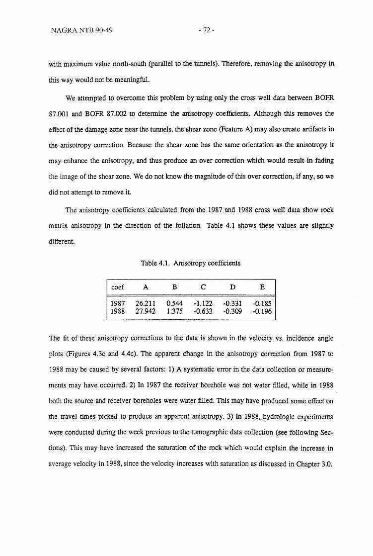
NAGRA NTB 90-49 - 72-
with maximum value north-south (parallel to the tunnels). Therefore, removing the anisotropy in
this way would not be meaningful.
We attempted to overcome this problem by using only the cross well data between BOFR
87.001 and BOFR 87.002 to detemtine the anisotropy coe:fficients. Although this removes the
effect of the damage zone near the tunnels, the shear zone (Feature A) may also create artifacts in
the anisotropy correction. Because the shear zone has the same orientation as the anisotropy it
may enhance the anisotropy, and thus produce an over correction which would result in fading
the image of the shear zone. We do not know the magnitude of this over correction, if any, so we
did not attempt to remove it
The anisotropy coefficients calculated from the 1987 and 1988 cross well data show rock
matrix anisotropy in the direction of the foliation. Table 4.1 shows these values are slightly
different.
coef
1987 1988
Table 4.1. Anisotropy coefficients
A
26.211 27.942
B
0.544 1.375
c D
-1.122 -0.331 -0.633 -0.309
E
-0.185 -0.196
The fit of these anisotropy corrections to the data is shown in the velocity vs. incidence angle
plots (Figures 4.3c and 4.4c). The apparent change in the anisotropy correction from 1987 to
1988 may be caused by several factors: 1) A systematic error in the data collection or measure-
ments may have occurred. 2) In 1987 the receiver borehole was not water filled, while in 1988
both the source and receiver boreholes were water filled. This may have produced some effect on
the travel times picked to produce an apparent anisotropy. 3) In 1988, hydrologic experiments
were conducted during the week previous to the tomographic data collection (see following Sec
tions). This may have increased the saturation of the rock which would explain the increase in
average velocity in 1988, since the velocity increases with saturation as discussed in Chapter 3.0.

NAGRA NTB 90-49 - 73 -
Although it is not likely that the background anisotropy changed from 1987 to 1988, the
anisotropy was removed from each data set using their respective correction coefficients. In each
case the contribution of the anisotropy was calculated and removed from the observed travel
times. This was done by calculating the difference between the travel times calculated with
coefficients A-E and the travel time calculated with only coefficient A, and then subtracting this
value from the measured travel time.
The travel times corrected for anisotropy were inverted in the same fashion as the
uncorrected data. The effect of the anisotropy corrections on the 1987 results (Figure 4.10)
change the magnitude of the anomaly corresponding to the shear zone. The corrections also
cause the amplitude of the anomaly to vary along the strike of the main fracture zone. Also,
smaller zones within the large low velocity feature adjacent to borehole BOFR 87.001 are more
resolved and coincide with similar features in the 1988 result.
The result of applying the correction to the 1988 data is shown in Figure 4.11. The
uncorrected image has been smoothed with the low velocity zones more distinct. The inversion
also appears to remove some artifacts that are produced in the original inversion. The smearing
seen to the upper left of Figure 4.9 is reduced, as is the effect of a strong, thin low velocity feature
extending from the middle of the laboratory tunnel to the center of BOFR 87.001. The "secon
dary" features which parallel the main low velocity zone (Feature A) in Figure 4.9 are also
greatly reduced leaving a single zone whose intersection with the laboratory tunnel coincides
with the large fracture observed on the wall of the AU tunnel.
4.4. Cross Well Studies
In many field cases only the cross well ray paths can be obtained. This maybe due to the
damaged or weathered zone preventing adequate surface to borehole arrivals or simply lack of
access. At FRI we see a damaged zone associated with the tunnel which strongly affects the wave
amplitudes, thus affecting the quality of the travel time picks. In order to determine the
effectiveness of cross well data to image the region between the boreholes we inverted only the
cross well travel times. Because the 1987 and 1988 differences are greatest in the regions of the
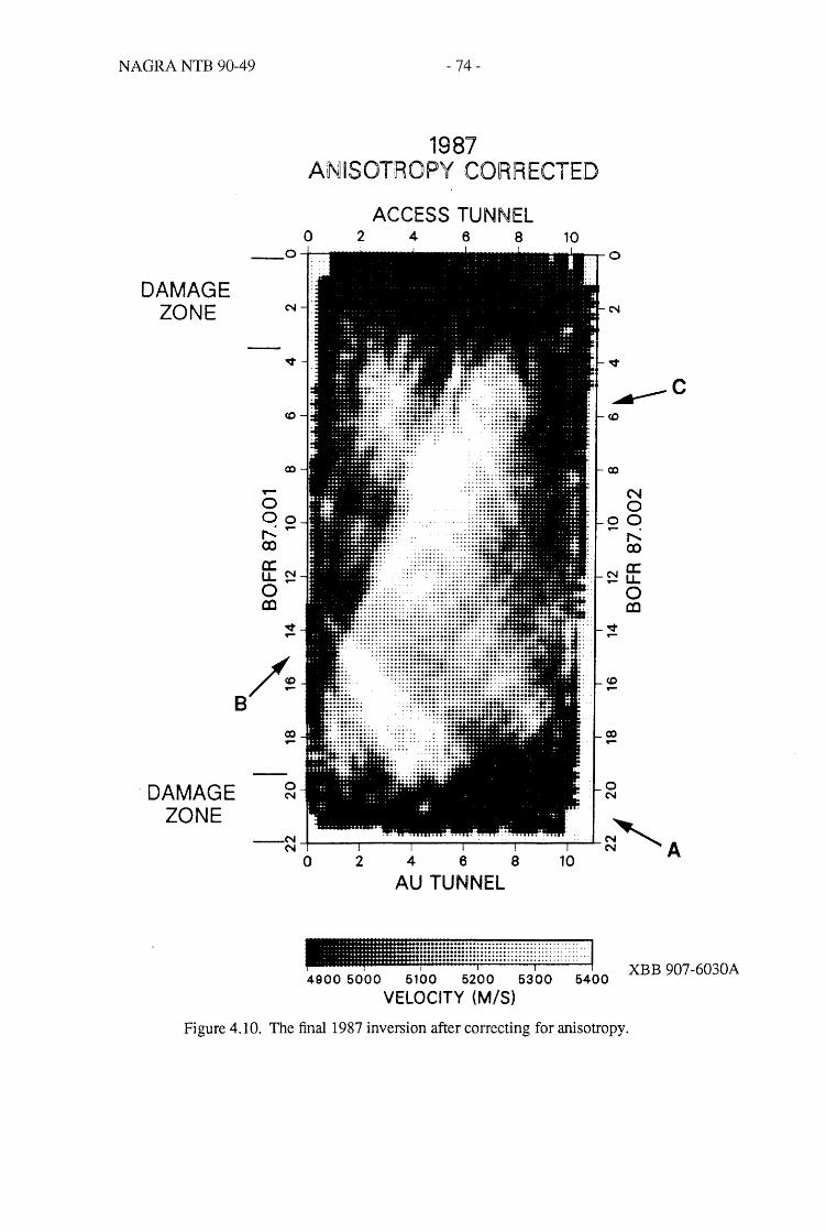
NAGRA NTB 90-49
DAMAGE ZONE
. DAMAGE ZONE
- 74-
1987 ANISOTROPY CORRECTED
ACCESS TUNNEL o 2 4 6 8 10
....---c
co -
-+----r-----,---r----r------r-~ ~" A o 2 4 6 8 10
AU TUNNEL
4900 5000 5100 5200 5300 5400 XBB 907-6030A
VELOCITY (MIS)
Figure 4.10. The final 1987 inversion after correcting for anisotropy.

NAGRA NTB 90-49
DAMAGE ZONE
8
DAMAGE ZONE
- 75 -
1988 ANISOTROPY CORRECTED
ACCESS TUNNEL o 2 4 6 8 10
___ O4---~----~--~ ~~~:::::::::::::;:i~~~i~~i~:~:~~ :' ..
o : . : : ~~: ~ ~~~:: : :::::: : :: :::: ' : : ::
~ IIIII: .,'1I ~1!::I·' .....• , ... N
.:L>~n~~\[~l1t ..•....... , ....... ,' ....... . ....... .... .
~ ............. . :: ~~n[il:~i[U~liUtI)! ~ : ~~~:ii: ji~iH~mHiHHH::
CD
~ CD -o N
.. =::~::~::~::mmimm:::: ~ C
,..:Iilllw,il ~ . ::.:: ::::ffi:::aF.::
:~I!I~I!g to N
,,::::::m!!lli~!m 52 ~
...••..••... ,.. . ..... . . ..••...•.................. .. ........ .... . .. ..... .. -......... " .. " ..... . . ......... . .. . .......... . .. .......... .. ,., .. . ......... .... .. ..... .,. ..... ".
co Na:: _u.
CD -o N
o co
~ -t-;.....;.;.;..;..;.....;.;..;,;...;...;..;.;..;..;..;..;..;.;.~;..;..;..;.;.;..;..;,;..;..;..;....;.;.~~..;.;.;..;..;.;~~~ A o 2 4 6 8 10
AU TUNNEL
... :::::: ::::::,:; .. . . ........ ... ........ . ::: ::::::::::::::::!
4900 6000 6100 6200 6300 6400
VELOCITY (MIS) XBB 907-6031A
Figure 4.11. The final 1988 inversion after correcting for anisotropy. The "unusual" rays have been deleted.
NAGRA NTB 90-49 - 76-
tunnel, we expected the cross well images to be more similar when the rays sampling areas adja
cent to the tunnel are removed.
Initially the 1987, and 1988 cross well travel times were inverted without removing the
anisotropy (Figures 4.12 and 4.13, respectively). Compared to the 1987 cross hole results, the
1988 cross hole image is much "smoother" and has a higher average velocity, 5.26, than the
1987 image, 5.09. These images also show that the inversion is strongly affected by the back
ground anisotropy. In this crosshole geometry, the rays traveling from the upper part of BOFR
87.001 to the lower part of BOFR 87.002 are in the high velocity direction of the anisotropy, with
the other rays perpendicular to this direction being in the "slow direction. tt This creates a pat
tern of velocity values symmetric about an axis in the direction of the anisotropy. The result is an
excellent example of what happens when the anisotropy of the background medium is ignored.
We removed the background anisotropy as before and performed an inversion of the
corrected crosshole values for the 1987 (Figure 4.14) and 1988 (Figure 4.15) data. Note that
Features A and B seen in the four-sided images (see Figures 4.8 and 4.9) are not imaged in the
cross well results. These anomalies are unresolvable because they occur near the tunnel walls
where only horizontal rays sample them in a cross hole configuration. The images do show a low
velocity zone corresponding to a fractured area seen in the core logs at about 7 and 15 m down
from the access tunnel in borehole BOFR 87.001 and 15 m down borehole BOFR 87.007. The
orientations of the imaged zone agrees with the general orientation of the fractures.
The only real difference in the two crosshole results is that the velocities in 1988 are much
higher than in 1987. We feel that these differences may be attributed to the saturation of the rock,
coupling of the sources and receivers to the borehole walls, the different sources, and/or the qual
ity of data. Note that in Figure 4.2 (1988) the initial arrival is taken to be a small downward
pulse. In Figure 4.1 (1987) the downward pulse exists for only a few of the traces, so that the ini
tial arrival was often taken at the second zero crossing, thus resulting in later picks. In effect we
see a combined amplitude-velocity effect on the 1987 data, and mainly a velocity variation in the
1988 data.

NAGRA NTB 90-49 - 77 -
8
o
1987 CROSSWEll DATA
ACCESS TUNNEL 2 4 6 8 10
o -+-_~ __ ~_~ __ .....L..-_---J. __ 0
N ..... .
CX)
~
0 00 ,,-CO
C:::N LL_
0 CO
.q--/~
CX) -0 N
N N
............
......... -
...---c
N o
00 -~
CO
Na: _u.
o N
o m
4-----,.2~-"""T4--"""T6.:........:.......;...;.....;.· ·.;..;,.8....;.·;,.;..;.· ··.;.;.;.···.;.....;.;,.10...;.;....:...;L~ A 0
AU TUNNEL
.... -.............. . . . ............... . .. .............. . . .. .............. .. ..... ............... . .. , ............. . 4900 6000 6100 6200 6300 6400
VELOCITY (MIS) XBB 907-6032A
Figure 4.12. Cross borehole data inversion of 1987 data, no anisotropy correction.

NAGRA NTB 90-49
o
- 78 -
1988 CROSSWEll DATA
ACCESS TUNNEL 2 4 6 8 10
o 0
.......................... ........................... ........... .
................ , ....................... . ..................... , ...... , ...... ' .... . ......... ......... . ............... ....................... ............. . ..........• .. ........... , ........... . .. .. , ..................... .
•••• •• •••• • •••••••• ·m::W~1!1W··· ... : ....... : ~ . : : : . : : : : : . : : : : . : : :n n H mr'
<0 .. : .......... ::::.:.::.:.:.:.:::::::::::::
.. .. . ~ .. ..... . . : ::::~~~!~~~·m:~~~mm III~_
... • • ..;: mlllll::~1 gO··········: imm~l~W:T·.:::::::::::lmmm~~ I~I~II~ ,....: - ::::::::::::::;;::::::::;:::::::::m~~m::
N o
00 -,...: co
CO H~!!:~!!%!!!;!!!l~ i ill j j j j l ~ll~~~j 1~ ~ (l j i ~! ~ j ~ 1 ~j j ~iij m~~~~L:::::::::: a: N :::::::::::::::::::::.:::::::::::::::: ::::::::::::::~;;;: N a:: LL _ ::::::::::::::::::::::::::::::::::: ::::::::;::::;;;::: _ u..
~ ~ ::::l~~illlll;!!II!!lmlllli!!i!!!!!!!l!:'!·I·!' ~ ~ e/: ;iiiiiiiiii.i:i:' .i.:; JIII!::.IIIIII!I I III 11
111111
':: i :
o N
-:.:::;:::::::::::::::::::::::: 0
N
~ -+----,.--..,.----,-.-.. '-" '-" -" ''T"'''-'' '-" '-"-' .,... .. '-' '--~ A o 2 4 6 8 10
AU TUNNEL
. ::::::: ::::::: ... ... ..... .........•
.: ::::::::::::::: ... XBB 907-6033A
4900 6000 6100 6200 6300 6400 VELOCITY (MIS)
Figure 4.13. Cross borehole data inversion of 1988 data, no anisotropy correction.
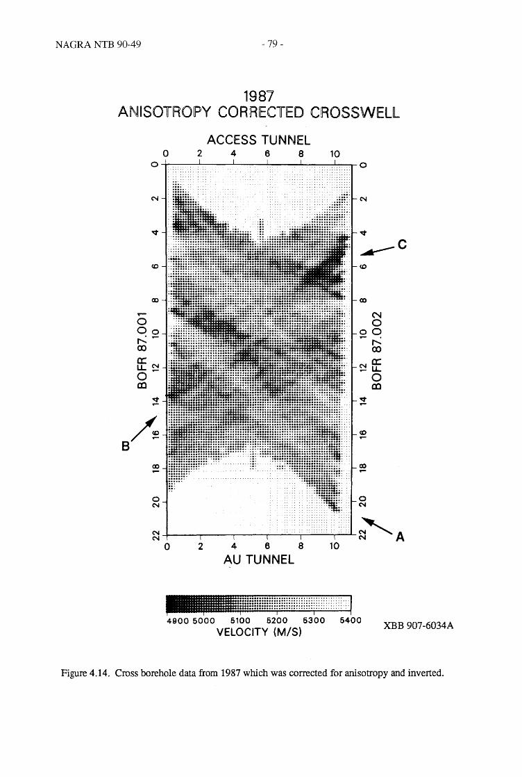
NAGRA NTB 90-49 - 79-
1987 ANISOTROPY CORRECTED CROSSWELL
ACCESS TUNNEL o 2 4 6 8 10
CD
~
0 00 ,....:-CX)
a:N u._
0 al
~ -
8 ~
CD -..
0 N
N N
0 2 4 6 8 10
AU TUNNEL
4900 6000 6100 6200 6300 6400
VELOCITY (MIS) XBB 907 -6034A
Figure 4.14. Cross borehole data from 1987 which was corrected for anisotropy and inverted.

NAGRA NTB 90-49 - 80-
1988 ANISOTROPY CORRECTED CROSSWELL
ACCESS TUNNEL a 2 4 6 8 10
o-+----'---~---.l...--.l...----L-__ O
......... , ..... . · ............. . · ............. .
~mlmlll1,1,: ..... ···· · ................... , · .................... . .................... · ............................... .
::.:::::::::::::::::::::::: N : :::::::::::::::::::::::::::
. .': : : : : : : : : : : : : : : : :: ~ : : =: ! : : :
, ........................ ,.. • ••••••••••• •• t ••••••••••••• ........................... ,. . .................................. . · " " .................... . . .......................... . · .................................................................... -~ . :.::::::::::::::::::::::;:::::::::.: ... ::::::::::::;::::::::::::::::: ~
· ................................................................... . ........................... . ............................ C .................................. , ................................ .
: .. ~::::::··::~!TTl~~n!T·:l~~L:;;~inlniH~U!n~HlHn~nT;: ~ <0 : : : : : : : ....... : : : : : : : : ; .. : ~ ~ : ~ ~ ~ ~ ~ ~ ~ ~ ~ ~ ; ~ ~ ~ 1 i ~ ~ 1 i ~ ~ ~ ~ ~ ~ ~ ~ ~ ~ ~ ~ ~ ~ : : : : : : : ~ : : : <0 .................................................. ................................................. .
.. ::: ::~ :::... :: ~!! iii ~ i i:: i ii ii i ii i i ii iii iii! i! iii ii i iiii~~lm!~ i: co .... ::::::::: .... :::::::::::::::::::::::::::::::::::::::::::::::':: co
go •.• ;"" •• 1 1 1~1~!!~wJ11~1;1 ::11· ...... 1·1:
1
·1111111Iilllllllllllll'· •••
;: .il~!!!~lll:li:. :.:! i ii ii:l11.11l:i!iiili· i1ili!I j Iii·, I!! 11!1:·!f·.l •• ~;;;~~;~~ ~~~g~~;~~~i~~~~~ ~ ~. ~ ~ ~ i ~ ~~~g~;!!~~~~~~~~~~~~ ~ ~ ~ ~ ~ ~~ ~ ~~~~~~ ~ ~ ~ ~:
N o 00 -,....:
CX)
Na: _u-o al
;. 1:lllllllllllllli!III!11 ,llill1: .. j; .;;.:: 1.:::1111111111 111111111 ii:; ;... :
B ~ ii·· i·:·· il i :.1::: Ill! II 1! m m: m!!!! II!I i II i III [II i! i 1111· ··"Iii! :
....................... ..... ................. . . . . .... ............... .. .. .. .................... . .. ..... .............. - .-
0 .. N
:::::::::::::::::::;;:: .. 0 :.::::::::::::::::::::::::. N ........................ . - ..... . .. . - ......... ,.
N N
-+-----r---.,..----,---: :-: :_.: :......,: :r-: :-:: :-:: :-: :..,. .. _ .. _ .. .a-~, A
0 2 468
AU TUNNEL
.::: :::: :::::::: .. . . .................. . ..................... .... ................. ... •••• a ........... .
10
4900 6000 6100 6200 5300 5400
VELOCITY (MIS)
XBB 907-6035A
Figure 4.15. Cross borehole data from 1988 which was corrected for anisotropy and inverted.

NAGRA NTB 90-49 - 81 -
4.5. Amplitude Tomography
In order to investigate the utility of using amplitudes for imaging the FRI zone we decided
to use the 1988 data to invert for attenuation infonnation. We felt that because no mechanical
clamping was used for the source, and only fluid coupling was used in the 1988 data, source and
receiver effects would be minimized.
The first arrival wave amplitudes may be inverted for the attenuation field using the same
inversion process used for the travel times through the equation
Ak r Pk = -In Ao = 'k.: aex,y)ds (4.2)
where Pk is the "projection" of the ray, Ak is the measured amplitude, Ao is the source ampli-
tude, Rk is the ray path, and a(x,y) is the attenuation at the x,y coordinate. Additional data pro-
cessing must be perfonned to properly detennine the amplitudes, and assumptions are made for
the cause of the dissipative mechanisms of medium. It is assumed that the measured amplitude is
a sufficient measure of the initial energy received and that the data can be corrected for the
geometric spreading and the source radiation pattern with the remaining energy dissipation due
to the intrinsic attenuation of the medium.
The wave amplitude, Ak, is considered to be a measure of the received energy and is usu-
ally measured from the peak-to-peak. or zero-to-peak amplitude of the initial arrival. A compar-
able value is the square root of the power, which is a more stable parameter. The power is deter-
mined by the fonnula
N P= L~tIA(i)l/N (4.3)
i=l
where ~t is the sample rate, A(i) is the amplitude at time i, and N is the number of samples in the
specified window. We took a window of 66 samples, or 0.264 msec, i.e., the initial arrival to
about one and a half cycles. The total energy from all three components were added to detennine
the total energy.
The amplitude values must be corrected for geometric spreading and the radiation pattern.
NAGRA NTB 90-49 - 82 -
The geometric spreading correction simply multiplies the amplitude value by the distance trav-
ele(t The radiation pattern is assumed to be a cosine function with 9 measured from the horizon-
tal. The actual radiation pattern was checked by performing measurements in boreholes BOAU
83.002 and BOAU 83.003 to the south of the FRI site. The geologic logs of these boreholes show
no fractures or anomalous zones between 5.0 and 10.0 m down each hole from the access tunnel.
In order to accurately determine the radiation pattern of the source, the attenuation, a, of the rock
must be known. A simplistic method of determining a is to take two measurements at two
different source-receiver offsets and apply the formula:
a- In --1 [A(XI) 1 - X2 - Xl A(X2)
(4.4)
where Xl and X2 are the two offsets and Al and A2 their respective amplitudes. We again calcu-
late the amplitude from the power formula., For the source-receiver offset, we used the path
directly across boreholes BOAU 83.002 and BOAU 83.003, a distance of 1.0 mat 9 = 0°. For this
offset, Al = 15402 and Xl = 1.0. Source-receiver offset A2 was taken from across boreholes
BOFR 87.001 and BOFR 87.002, a distance of 10.0 mat 9 = 0°. Although there were a total of 40
direct crosshole measurements taken between these boreholes, most of the ray paths intersect at
the fracture zone. Because only the background attenuation is wanted, the values for the five
largest amplitudes were calculated and averaged. In this case, A2 = 1300 and Xl = 10.0. Apply
ing Equation (4.2), a becomes 0.3 m-l . We calculated the Q of the medium by using the equation
1tf Q=av
(4.5)
assuming a velocity of v = 5200 mls and frequency f = 6000 Hz, a value of about 12 was obtained
for Q. BecauSe the ray paths were not common, Q becomes relative.
The radiation pattern for the source was obtained by plotting the observed amplitudes
A(x,8) with the calculated amplitudes Ao(x,9) = e-<IX for several angles, and fitting the resulting
curve with an angular function. The values used are from the tests carried out between boreholes
BOAU 83.002 and BOAU 83.003. The amplitudes are plotted in Figure 4.16 along with the
values for a cosine function. As expected, the values fit closely to the cosine function. The

w 0 ;:) ~ :J c... ~ et: w > ~ ..J W a:
NAGRA NTB 90-49 - 83 -
0.98
0.8~
0.72
o.eo
0.~8
0.38
b-
0.24 0 b-
b-
ee 0.12 0
0 0
0
0.12
POLAR PLOT OF RADIATION PATTERN
b-
0
0.2~
0 b-
o - MEASURED VALUES b- - COSINE AT
0
0.38 0.~8 0.80 0.72
RELATIVE AMPLITUDE 0.8~ 0.98
XBL 907-2523
Figure 4.16. Measured radiation pattern of the 1988 source.

NAGRA NTB 90-49 - 84-
difference may be due to a slightly erratic value for a and the attenuation anisotropy of the
medium. The amplitudes were then corrected for the radiation pattern by dividing each value by
cos e.
The source amplitude, Ao, is a difficult parameter to determine. The effect of having a poor
value is the same as neglecting a constant time correction when inverting travel time values. 1bis
usually results in excessive smearing and false anomalous zones. One method of estimating the
source amplitude is to solve Equation (4.2) for A(x=O) gi~en a:
(4.6)
Using X2 = 1.0 m, A(X2) = 15402 and a = 0.3 m-1 the source amplitude becomes 21000. 1bis
value was used for Ao in Equation (4.1).
The same inversion routine was used to invert amplitude data as was used. to invert travel
time data. The amplitudes were calculated and corrected for each source-receiver offset, produc
ing the same number of data points as for the travel time inversion.
The inversion was first perfonned on a 33 x 66 pixel map (Figure 4.17). The shading ranges
from 0.31 m-1 (dark) to 0.28 m-1 Oight) agrees with our calculated value of 0.31 m-1 for the
background anisotropy. The values obtained in the inversion range from about 0.22 m-1 in the
central region to about 0.65 m-l in the damaged zone near the tunnel walls. As can be seen from
Figure 4.17, this damaged zone dominates the image so that smaller anomalies are not evident.
The only additional anomaly that is observed is located near the 10 meter point of borehole
BOFR 87.001. This position coincides with a large velocity anomaly, the intersection of feature
A and B, seen in the velocity tomogram (Figure 4.11).
An inversion was done with only the cross borehole rays to eliminate the contribution of
the damaged zones to the result. This image (Figure 4.18) produces other anomalies, but the lim
ited angular coverage and the large reduction of data seems to lead to some smearing. Using the
crosshole data, the anomalous zone near the 10 m point of borehole BOFR 87.001 is more dis
tinct Other zones near the boreholes also coincide with highly fractured areas or with the velo
city results. However, the large zone extending from the intersection of BOFR 87.002 and the

NAGRA NTB 90-49
DAMAGE ZONE
DAMAGE ZONE
o
o
- 85 -
1988 CROSSWEll AMPLITUDE
ACCESS TUNNEL 2 4 6 8 10
246 8 ------~A 10
AU TUNNEL
0.31 0.30 0.29 0.28 XBB 907-6036A
ATTENUATION (11M)
Figure 4.17. Result of inverting the 1988 amplitude data.

NAGRA NTB 90-49 - 86 -
DAMAGE ZONE
o
<0
'r""
o
1988 CROSSWEll AMPLITUDE
ACCESS TUNNEL 2 4 6 8 10
.. :.::::: ... ::.. CD
" ... ~ .
o 0 1· ••• 0; ....... ;;;;.;; .. ;~I: . . .. . ...... .-, ..... ::' .. ':: :-:':::: .. :.: ... .
N o
00 -r'
co r'co
- ........................ . : : :: :- :::',:-:: :: :: ... ", ........................ .
:. :: :: ,::::::::.::. ~: . : a: N u._
. :: :: :' .:: .. ::: ... : ..... . Na: .-u.
o III , '::::::::::::::::::::::::::::::
~ .::::::::::::::::::::::::::::::::::::: ~
~ .......................'".,::,:"...mmm: ~
B ~ •••••••••••••••• : ••••• ! •..... :111. ,0:. ... J !I·!;· :.ll:!· .. ·I ... : .t.:.!. :~ ... ;.l .. :;' .. :.:. '.:. :.:' .... ! .. ::: ... 1..;.'.: ..... : ,~ .. ;: .•. :. ~ - :.;;;;;;;,; .. ;;:::::::::::: ::...... ............... ~
o N
•• ; • ; : • : : ••.•. : ; ; ; ; • : : 7 ~ : : . : ~ , • ~ : •
...................••... . .. . .... .., ........... , .......... ..•....
o N
o al
DAMAGE ZONE ~ -+----,.------..,----~ .. ~ .. ;.;.;.. .... ~.::..;..;...;: :..;..;...;:::p.;..:.:::..;.;..;.:::.;.;..;.:::.:..:...;.: .. :..;.:..;.:.:~:::..;.L' ~'A
o 2 4 6 8 10
. . : : : : : : : : . : : . : : . : : : : : : :: :::' ~ ~ ~ : .
AU TUNNEL
0.31 0.30 0.29 0.28 XBB 907-6037A
ATTENUATION (11M)
Figure 4.18. Result of inverting the 1988 cross borehole amplitude data.

NAGRA NTB 90-49 - 87 -
access tunnel does not coincide with any other velocity or geologic feature except at the intersec
tion itself. This anomaly seems to be due to a smearing, i.e. low ray coverage, of this known frac
ture zone toward the main anomaly, Feature A.
The attenuation results do not substantially improve our knowledge of the FRI region. They
suggest that the most important feature besides the damaged zones is the low velocity/high
attenuation anomaly near the middle of borehole BOFR 87.001. This zone is strongly identified
in all the images. The cause of the feature is probably some intersection of fractures and/or lam
prophyres.
However, the results do support the stifihess theory at these frequencies. The time delay
produced by a large number stiff fractures would be negligible at these frequencies, but the
attenuation effects would be significant This is dependent on the number of fractures and the
stiflhess value. These parameters are unknown, but the damaged zone probably contains a large
number of microcracks. The attenuation results also support the theory that the 1987 velocity
tomogram is an effective combination of velocity and attenuation effects. The attenuation meas
urement would have yielded much more information if we had used a data collection system with
more dynamic range. Our system was a 12 bit system. A 16 bit system would have provided 16
times more contrast in amplitudes, thus providing a wider range of amplitudes to analyze.
4.6. Discussion of Results
Although not immediately obvious, after anisotropy corrections, the 1987 and the 1988
results show essentially the same features. We will first discuss how the two results compare,
then analyze the best image in terms of what is known of the geology in the FRI site.
An obvious difference between the two results is the disappearance of the low velocity
features near the tunnels in 1988 results (Figures 4.10 and 4.11). Because these features were the
most dominant anomalies in 1987, a satisfactory reason must be found to explain its disappear
ance. As previously stated, the data quality was much better in 1988 than 1987 for several rea
sons. The source was more powerful and its repeatability improved. Also, when the source and/or
NAGRA NTB 90-49 - 88 -
receiver were in BOFR 87.(X)1 and BOFR 87.002 the coupling was improved over 1988 because
both holes were water filled. We also stacked from 2 to 9 traces for each source receiver pair.
These improvements increased the signal to noise ratio providing much more accurate travel time
picks on higher frequency first arrivals. In effect. the reduced data quality in 1987 prevented the
"proper" first arrival travel times to be picked in 1987. In some cases the value picked was a
pulse or two later than the time picked in 1988. TIlis is especially true where the attenuation is
greater, e.g., the damaged zones adjacent to the tunnel and in the main shear zone. The entire
1987 travel time data for sources or receivers along the tunnels are probably picked consistently
late, producing a velocity reconstruction which shows consistently lower velocities near the tun
nels and resulting in a lower average velocity. TIlis means that the 1987 tomogram was essen
tially a mixed velocity-attenuation tomogram.
Another difference in the results is that the shear zone (Feature A, Figures 4.10 and 4.11)
becomes discontinuous and less dominant in 1988. TIlis result is of great interest because this is
the zone that we were initially trying to image. Also, Feature C is less obvious in the 1988
results, again a target of the hydrologic tests. In 1987, we had assumed that we had imaged
Feature A satisfactorily as a several meter wide low velocity zone. However, the 1988 inversion
does not show such an extensive feature, but a thinner zone which extends to about 4 m from the
laboratory tunnel. The zone dies out for a meter, then reoccurs as a more massive feature with
variable velocity. To show the actual difference in the results, the 1988 image is subtracted from
the 1987 image pixel by pixel (Figure 4.19). (An inversion using the differences in travel times
could not be performed because slightly different stations were used for a few of the sweeps). As
can be seen from Figure 4.19, there is little difference between the two images except at the tun
nels, suggesting that the 1987 low velocity zone in the region of the shear zone and Feature C
exists in the 1988 result, but has a slightly different form and magnitude.
Both 1987 and 1988 images show a lower velocity near the intersection of the AU tunnel
and the shear zone where the excavation of the tunnel may have • 'loosened" the fractures. The
large low velocity features toward borehole BOFR 87.001 on strike with the shear zone are also
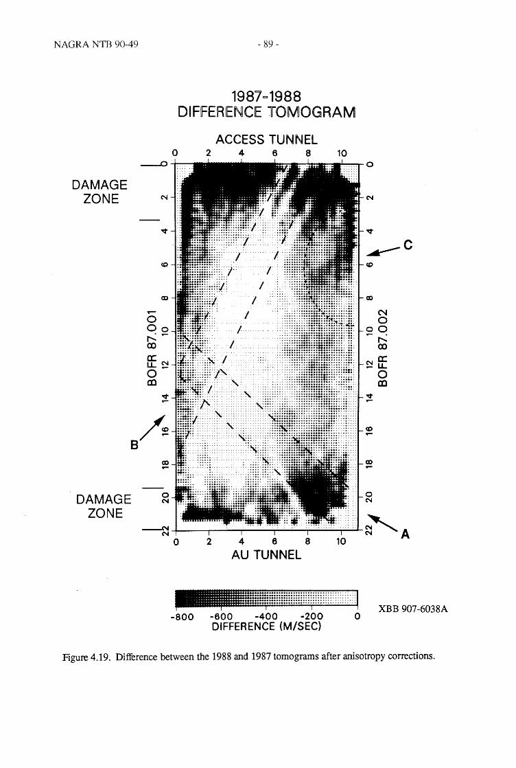
NAGRA NTB 90-49
DAMAGE ZONE
8
DAMAGE ZONE
a:N u.._
o al
~ ex) -
o
- 89 -
1987=1988 DIFfERENCE TOMOGRAM
ACCESS TUNNEL 2 4 6 8 10
o
~c
ex) -o N
~---",----"';-";"'---:'-~':"""":':"~";';";";";':":"':";";'':'';':'';''';'.;L..~A o 2 4 6 8 10
AU TUNNEL
-800 -600 -400 -200 o XBB 907 -6038A
DIFFERENCE (M/SEC)
Figure 4.19. Difference between the 1988 and 1987 tomogramsafter anisotropy corrections.
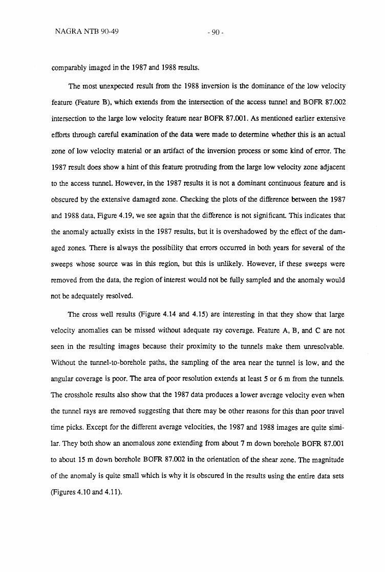
NAGRA NTB 90-49 - 90-
comparably imaged in the 1987 and 1988 results.
The most unexpected result from the 1988 inversion is the dominance of the low velocity
feature (Feature B), which extends from the intersection of the access tunnel and BOFR 87.002
intersection to the large low velocity feature near BOFR 87.001. As mentioned earlier extensive
efforts through careful examination of the data were made to determine whether this is an actual
zone of low velocity material or an artifact of the inversion process or some kind of error. The
1987 result does show a hint of this feature protruding from the large low velocity zone adjacent
to the access tunnel. However, in the 1987 results it is not a dominant continuous feature and is
obscured by the extensive damaged zone. Checking the plots of the difference between the 1987
and 1988 data, Figure 4.19, we see again that the difference is not significant This indicates that
the anomaly actually exists in the 1987 results, but it is overshadowed by the effect of the dam
aged zones. There is always the possibility that errors occurred in both years for several of the
sweeps whose source was in this region, but this is unlikely. However, if these sweeps were
removed from the data, the region of interest would not be fully sampled and the anomaly would
not be adequately resolved.
The cross well results (Figure 4.14 and 4.15) are interesting in that they show that large
velocity anomalies can be missed without adequate ray coverage. Feature A, B, and C are not
seen in the resulting images because their proximity to the tunnels make them unresolvable.
Without the tunnel-to-borehole paths, the sampling of the area near the tunnel is low, and the
angular coverage is poor. The area of poor resolution extends at least 5 or 6 m from the tunnels.
The crosshole results also show that the 1987 data produces a lower average velocity even when
the tunnel rays are removed suggesting that there may be other reasons for this than poor travel
time picks. Except for the different average velocities, the 1987 and 1988 images are quite simi
lar. They both show an anomalous zone extending from about 7 m down borehole BOFR 87.001
to about 15 m down borehole BOFR 87.002 in the orientation of the shear zone. The magnitude
of the anomaly is quite small which is why it is obscured in the results using the entire data sets
(Figures 4.10 and 4.11).

NAGRA NTB 90-49 - 91 -
4.7. Geologic Interpretation of the Results
The geologic map of the structures at FRI is shown next to the "final" 1988 tomographic
image to assist in the interpretation (Figure 4.20). To be useful the interpretation of the tomo
graphic images must include the geologic structure that is associated with each of the main
features that are imaged and an explanation for the differences between the results of the 1987
and 1988 experiments. These include:
1. The large low velocity anomalies observed along the tunnels in the 1987 image which
do not exist in the 1988 result.
2. The shear zone (Feature A) is observed in 1987 as a single large low velocity zone
about two meters wide. The corresponding zone in the 1988 results consists of a very
thin « 0.5 m thick) zone which become discontinuous.
3. Feature B, which extends from near the access tunnel BOFR 87.002 intersection, to
the middle ofBOFR 87.001, and is, in fact, the dominant feature of the 1988 results.
4. Two strong low velocity features at the intersection of Feature B and the shear zone.
We have already mentioned that the low velocity zones associated with the tunnels in the
1987 results may be due to the initial P-wave pulse being highly attenuated. This was primarily
due to a· weaker source being used in the 1987 experiment. However, this does not explain why
the 1988 velocity data did not resolve the damage zones, i.e., if there are damage zones with high
fracture content, why did we not detect them in the 1988 velocity data. It is true that one expla
nation may be that the 1987 result only detected the damage zone by picking later arrivals
because the initial pulse was attenuated, not slowed, and thus an artificially low velocity result
was obtained. The attenuation data from 1988, however, did detect the damage zones near the
tunnels. This suggests that at the frequencies we used,S to 10Khz, the effect of these thin frac
tures on the velocity was much less than that on attenuation. This is in fact what the "stifIhess"
theory predicts. As frequency increases, for a constant stifIhess, the velocity or delay becomes
less relative to the attenuation effect. Apparently we were at frequencies where for the stifIhesses
involved, attenuation is important and delay is less important.
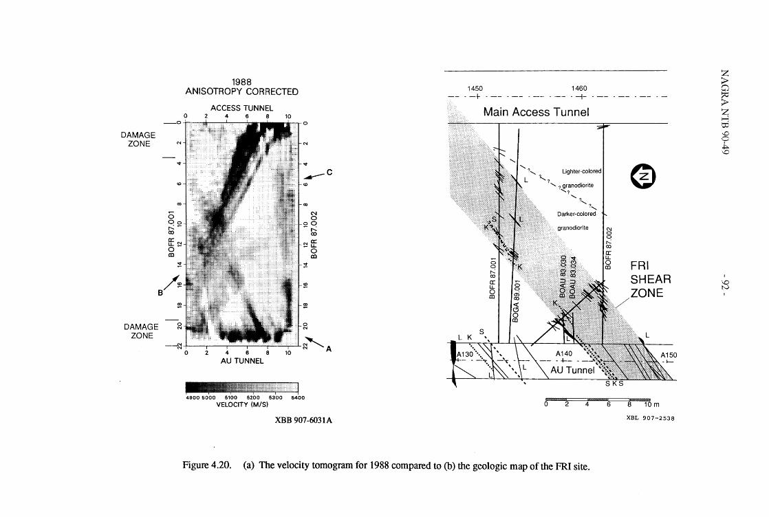
DAMAGE ZONE
B
DAMAGE ZONE
1988 ANISOTROPY CORRECTED
ACCESS TUNNEL o 2 4 6 8 10
__ 0 I .J. o
N
q-
<Xl
0 00 r..:~
co
fE~ 0 al
~
/~ e:!
0 N
~ 0
N
q
::::," :::::r-~
~
e:!
o N
4 ~ ~ ·:i·'~ i
AU TUNNEL 10 A
_iiif:iiiif:mllHlHlHH+i:::::H:::: ., 4900 6000 6100 6200 6300 6400
VELOCITY (MIS)
XBB 907-6031A
1450 1460 --~ --- --- --- --- -~-
Main Access Tunnel
'? Lighter-colored
., ? granodiorite .'?
o
., ? ., ?,
Darker-colored
2 4
Figure 4.20. (a) The velocity tomogram for 1988 compared to (b) the geologic map of the FRI site.
C\I a a
" OJ
cr LL o CO
6
®
FRI SHEAR
E
8 10 m
XBL 907-2538
z > CJ ~ > Z @ I,() C ~ \0
\0 tv

NAGRA NTB 90-49 - 93 -
In the final 1988 tomogram, the shear zone appears to produce a relatively weak velocity
anomaly. The zone appears as expected from the 1987 results, but its form is altered in 1988.
Although there is a visual difference, the actual differences are not great and may be due to the
better resolution obtained in 1988. The 1988 results indicate that it is likely that the zone is not a
simple single planar feature and thus the permeability along the zone may also be variable rather
than being a single well connected feature. Figure 4.20 indicates that the shear zone produces a
large velocity anomaly near the AU tunnel wall, until the point where this anomaly intersects a
larnprophyre at about 4 m from the AU tunnel wall along the strike of the shear zone. The inter
sections of lamprophyres and shear zones are areas of more intense fracturing, probably causing
larger velocity anomalies. This lamprophyre is probably discontinuous, being stretched along the
shear zone during deformation. After this velocity anomaly dies out, another small low velocity
anomaly is encountered at about 2 m further along strike of the shear zone. This anomaly may be
another piece of lamprophyre or a region of high fracturing.
The most dominant feature in Figure 4.20 is Feature B, which extends from a highly frac
tured area in the access tunnel to the shear zone. It is unlikely that the anomaly is totally an
artifact of the inversion or due to data errors since it occurs in the results from both years. The
anomaly may not actually extend to the shear zone, but may be smeared somewhat in this direc
tion. The visible fractured area at the access tunnel where the anomaly begins consists of subhor
izontal fractures and a tension fissure. From geologic considerations, it is most likely that this
feature is associated with a lamprophyre or an especially large tension fissure. The strike is
different from the lamprophyres in the immediate area, but as noted in the geology section, lam
prophyres are not consistent in their behavior, especially when associated with shear zones.
Since the geologic information about this feature is sparse, the only way to validate its presence
is to drill into it A subsequent borehole (BOGA 89.(01) was drilled parallel to BOFR 87.001,
but unfortunately it was several meters away from the anomaly and could not validate the predic
tion.
Where Feature B intersects the shear zone, Feature A, two large anomalies are also

NAGRA NTB 90-49 - 94-
observed. These anomalies may be areas of intense fracturing, most likely due to lamprophyres
intersecting the shear zone. A smalliamprophyre was logged in borehole BOGA 89.001 (Table
2.1) which coincides exactly with one of these anomalies. The other anomaly coincides with a
kakirite zone which also indicates a region of increased fracturing. These anomalies also suggest
that there may be hydrologic communication across the shear zone in this region.
Except for Feature B, all the anomalous velocity zones are coincident with geologic struc
tures. Feature C is still not verified, but the core suggests a different rock type, lighter colored
granite, rather than fracturing may be the cause of this feature. Although the core from this
region were not tested, the testing of the other core from the FRl zone suggested that the lighter
colored granite has lower velocity than the more altered darker colored granite (Chapter 3). The
two low velocity anomalies near borehole BOFR 87.001 were interpreted as zones of intense
fracturing likely due to the presence of lamprophyres. Borehole BOGA 89.001 was drilled, and
validated this interpretation. Though the geologic information determined the possibility of such
fractured regions, these anomalies could not be located by geologic data alone. It is always possi
ble that feature B could be an artifact caused by some data error. However, there is no basis on
which to reject its existence since it is observed in both the 1987 and 1988 results. Direct exami
nation leaves little doubt that there is some anomalous zone that exists near the tunnel wall, prob
ably a tension fissure.
Overall, the tomographic inversions seem to successfully image the major structures in the
test region. At the frequencies used, the tomograms do not successfully image the minor struc
tures such as individual fractures. The main conclusions from these tests are:
1. The velocity anomalies observed associated with fracturing were not due to single
fractures but groups of fractures.
2. The seismically important features associated with fracturing were fracture intersec
tions and fracture-Iamprophyre intersections. These are also the structures that should
be hydrologically important

NAGRA NTB 90-49 - 95 -
3. An interpretation of the results can not be done adequately without knowledge of the
geology.
4. Structures were resolved that could not be anticipated from the borehole and tunnel
data.
5. Although shear wave data were sparse, it is obvious that given the proper source, S
wave data would greatly aid in the interpretation of the geologic features.
6. The seismic visibility of the features from the amplitude and velocity tomograms
seem to support the stiffhess theory.
NAGRA NTB 90-49 - 97-
5.0. HYDROLOGIC ANALYSIS OF FRI EXPERIMENT
5.1. Introduction
Geophysical methods can be used to obtain useful infonnation for characterization of
underground geologic systems. The next step is to assess the hydrologic significance of the
features identified by the geophysical methods. Geophysically significant features are not always
hydraulically important and vice versa. In seismic methods, attenuation and velocity are meas
ured as a seismic wave travels through a rock. In other words, it is a point to point measurement
of the mechanical properties of the rock. On the other hand, hydraulic behavior is not entirely
governed by the mechanical properties of a rock, although it is closely related. It is the connec
tivity of the void spaces that controls the overall hydraulic properties.
At the Grimsel test site, LBL and Nagra designed hydraulic tests in conjunction with the
seismic tests described in the previous chapter. The tests were conducted by the company
SOLEXPERTS AG under the supervision of Nagra. In this chapter, we will describe how the
information obtained by geophysical investigations was used to design hydrologic investigations.
We will then discuss the hydraulic results and analysis of the hydraulic tests. In particular we
will focus on the anomalous interference data and attempt to find an explanation for it We will
also try to relate the analysis to seismic and geomechanic test results.
5.2. Background
5.2.1. Constant Pressure vs. Constant Rate Test
As a background we will briefly describe constant pressure tests, which were the type of
tests conducted at FRI site. In a constant pressure test, the hydraulic head in an isolated interval
is kept constant and the transient flow rate at the interval as well as pressure reaction in adjacent
intervals are monitored. In most groundwater applications, however, constant flux tests are more

NAGRA NTB 90-49 - 98-
commonly used because in moderate to highly permeable rocks, it is generally easier to achieve
and maintain a constant flux, q, than a constant pressure from the onset of the test. Therefore,
analytical solutions are more readily available for constant flux tests. The majority of the pub
lished papers in the literature are based on constant flow rate tests. Constant flow tests are also
easier to analyze because the type curves have somewhat more distinct shapes compared to con
stant pressure tests. In the latter, the type curve matching of q vs. time data from the pumping
well is less difficult because the curves are more or less flat. In analyzing constant pressure
crosshole tests, pressure vs. time type curves have to be developed for each observation well at
different radial distances. This is because the constant pressure solution is not similar in Kt/Ss ~.
The constant rate boundary condition is in general mathematically easier to work with to develop
a new analytical model.
However, constant pressure tests do have advantages. In very low permeability rocks, like
the one at Grimsel test site, constant pressure is generally easier to achieve than a constant rate.
It is also easier to minimize the wellbore storage effect in a constant pressure case. Moreover,
because the rock near the wellbore is subjected to a constant pressure throughout the test, there is
less concern about the permeability changing as a function of time (pressure). However, the per
meability may change in the location away from the well as the pressure front propagates into the
rock.
Whichever method is used, when conducting well tests in a tight fractured rock, it is impor
tant to measure early time data as accurately as possible. Transient data reflects the change of
permeability in space as a function of time. In this regard, transient data is more descriptive of
the rock heterogeneity than steady state data, which is influenced by the spatial arrangement of
heterogeneity in an unknown way. Especially when there is a skin zone near the well, one
should be able to evaluate the properties of the zone if there is good transient data for both the
flow period and the shut-in period.

NAGRA NTB 90-49 - 99-
5.2.2. Constant Pressure Solution
The dimensionless pressure in Laplace space for a constant pressure test with skin in an
infinite homogeneous two-dimensional system can be written as:
(5.1)
and for dimensionless flow, the solution is:
(5.2)
where p is the Laplace space variable, s is the skin factor, rD is the dimensionless radius, and Ko
and Kl are the modified bessel functions of the second kind of zero-th and first order, respec-
tively. The solutions in real space, hD and 'lo, can be obtained by inverting Equations (5.5) and
. (5.5) numerically (Figures 5.1 and 5.2). For references readers may consult Carslaw and Jaeger
(1945), Van Everdingen and Hurst (1949), and Ehlig-Echnomides (1979).
5.3. Test Configuration
The hydraulic tests were planned based on the 1987 tomography results (Figure 4.8).
Packer locations are shown on Figure 5.3. Each test consisted of pumping water in the interval at
a constant pressure and monitoring in all the other intervals. Objectives of each test were
1. to find hydraulic connection with other zones,
2. to characterize the properties of zones that are hydrologically active, and
3. existence of zones about which we have only inconclusive evidence.
The purpose of Test 1 was to provide a hydrologic characterization of a feature which is
clearly evidenced by geophysics. The packers for Interval 11.2 were placed such that they
confine the main fracture zone (corresponding to Feature A on Figure 4.8) as tightly as possible
in order to minimize wellbore storage and isolate the hydrology of the feature. Interval 11.2 was
used as the inflow interval and pressure was monitored in all the other intervals.
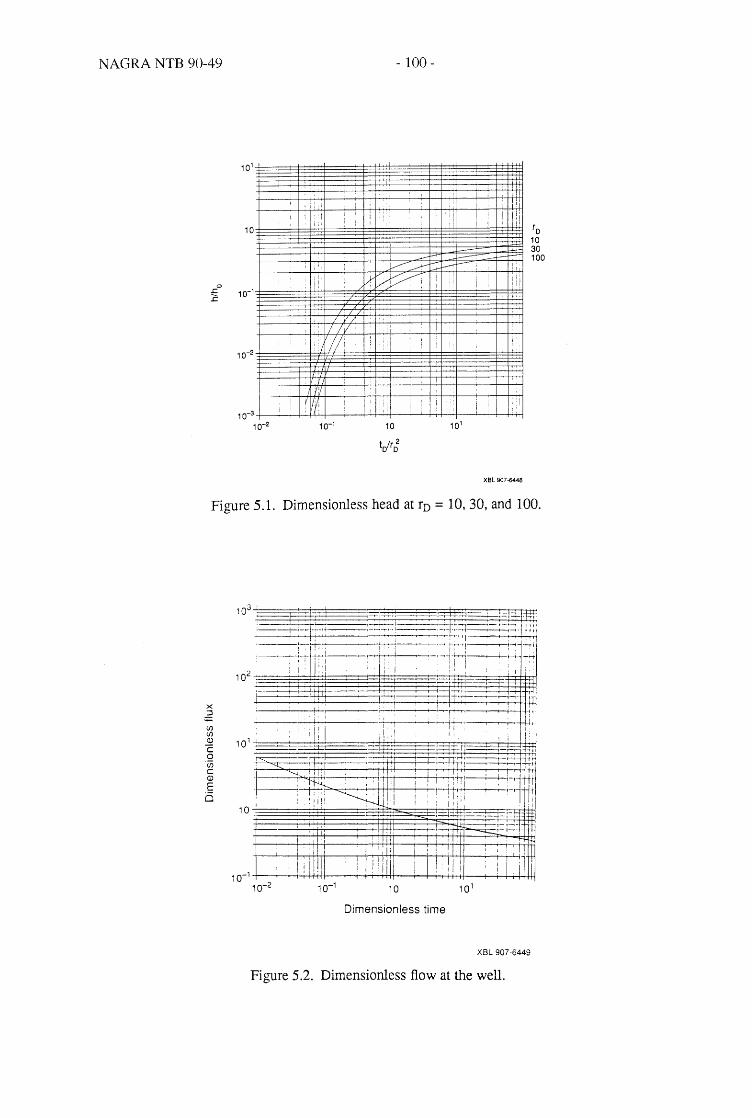
NAGRA NTB 90-49
o .c 1:
10-2
I
10-3
10-2
/ y;"
I II: il//
I tV
( ~l: 10-1
- 100-
:'
',I j
' I
:1: •
':
10 101
tD/r;
XBL 907-6448
Figure 5.1. Dimensionless head at rD = 10,30, and 100.
(Jl (Jl (l)
c o
"(i) c (l)
E (5
I I I:, : Ii! Ii!! I
! I 'I!il " i ! I: i: III I I !
10
Dimensionless time
XBL 907-6449
Figure 5.2. Dimensionless flow at the well.

NAGRA NTB 90-49 - 101 -
o o r-.: ex:> o co Upper access tunnel
P1.4
11.3
3
P1.3
11.2
P1.2
11.1
P1.1
Lower laboratory tunnel
_ Hydraulic packer
• Mechanical packer
Scale - -o 5m
~ ('j o M ex:> o co
C\J o o r-.: ex:> o co
P2.3
12.2
2
XBL 907-6450
Figure 5.3. Packer locations used in Tests 1,2 and 3 as of August 1988.

NAGRA NTB 90-49 - 102-
The purpose of Test 2 was to determine if the region to the north of 12.2 is hydrologically
significant This test would only have been conclusive if the result were positive. The tomogram
of Figure 4.8 showed this area to be a low velocity zones (Feature C). A negative result would
have meant that we did not find any connection between the low velocity region and any area
being monitored. A positive test result would have been very significant because this feature had
only been located with geophysics.
Test 3 was designed to understand the south-eastern part of the shear zone. Feature A
appeared clearly in the tomogram as extending across the tomographic plane. A parallel feature
to the south-east appeared in BOFR87.001 and in the BOFR87.002 core and nearby in the tomo
gram. However, the tomogram did not indicate that this part of the shear zone is continuous.
The test was designed to determine if there is continuity or if there is a cross-cutting fracture con
necting this part of the shear zone to 12.2 or n.1.
5.4 Test Results and Analysis
In the present report, we will focus on the results of Test 1. Comparison with the results of
Test 2 and 3 indicated that Feature A is clearly the most significant hydrologic feature at the FRI
site as expected. In Test 2, a coherent analysis is difficult because although 12.1 did take up some
water and a weak interference was observed in some intervals, some intervals were still recover
ing from Test 1. Therefore, there is no evidence that the low velocity zone to the north of 12.2 is
hydrologically significant. A similar conclusion can be drawn for Test 3 results. A weak but
definite hydrologic connection between Interval 11.2 and 12.2 was observed. Although the
existence of a cross-cutting feature cannot be completely denied, one can postulate that the
hydrologic significance is quite weak even ifit does exist. Readers interested in the details of the
test results are referred to Wyss (1988).
Figure 5.4 shows the pressure transient of interference data at various observation points in
Test 1. Note that the interval 13.1 responds most markedly. The response data at 13.1 is com
pared to the theoretical response obtained by evaluating Equation (5.5) at r = 10.2 m, or rn = 10.2
m/43 mm = 237 for s = 0 (Figure 5.5). As can be seen from the figure, the pressure observed at

NAGRA NTB 90-49
~ ell e ~ :::l en en a> 0:
3.0
2.5
2.0
1.5
L 1.0 ~ .....
0.5
o o
,7
10
- 103 -
-~
/ ~
-~ /"
L----
...-
Interval:
3.1
1.3 3.2 2.2 1.1 2.1
34.1
20 30 40
Time (hr)
XBL 907-6451
Figure 5.4. Interference buildup data for Test 1 at various observation points .
... . -~
~-
~ 10-2 -t-----f-f-----.,i'----+----+------l
J:
10-3T---f-~r-----+------l---------.j
10~+_~~~~r_.-~~~-~~~~~~~~ 10-1 10 101
Time (hr.)
XBL 907-6452
Figure 5.5. Comparison between data and the theoretical response curve.

NAGRA NTB 90-49 - 104-
13.1 is significantly lower than that predicted by the analytical solution, although the shapes of
the curves are almost identical. The analytical solution assumes that the fracture is infinite, iso
tropic and homogeneous. Therefore, conditions must exist where one or more of the above
assumptions are not appropriate. The plausible scenarios are:
1. Skin: There is a low permeability zone around the injection well, i.e., a skin that
causes the effective pressure at 11.2 to be lower.
2. Anisotropy: The fracture is anisotropic where the maximum permeability direction is
oriented vertically.
3. Leakage: There is leakage from the fracture to the adjacent rock so that the pressure
is more dispersed.
4. Boundary Effect: The boundary effect of the laboratory tunnel is keeping the pressure
low at 13.1.
In the following sections, more detailed discussions will be given for each case, although in real
ity all of the above conditions may coexist. As is the case with any field experiment, the possi
bility of an erroneous measurement should not be completely discounted. For example, the pres
sure loss through the tubing may not be negligible. However, we will limit our discussions to the
effects of the hydrologic features in the rock only.
5.4.1. Skin
Skin effect is usually suspected when anomalous results are obtained. Equation (5.5) can
be used to obtain pressure response curves at 13.1 for various values of skin factor, s. Figure 5.6
shows that the curve for s = 13 yields a relatively good match with the data except for the late
time portion. However, an almost perfect match can be obtained if the pressure in 11.2 is
assumed to be 6.6 bars, which is much lower than 19 bars (Figure 5.7). This is equivalent to
assuming that there is a constant pressure loss of more than 12 bars at the borehole wall. How
ever, this assumption contradicts the conventional skin concept where the pressure loss is
assumed to be proportional to the flow rate. Because the test was a constant pressure test, the

NAGRA NTB 90-49 - 105 -
8=0 5 10 15 20
~ 1Q-2+-----It--I-'-/.i!,.L--+-----+-----I
X
10-3+---+.ffli-.;.----f--------1-------l
104+-~~~*-~~~*-~~~~~~~~ 10-1 10
Time (hr.)
XBL 907-6453
Figure 5.6. Type curve match with the skin curves.
10-1 +-----+----;::II"!f-------!-------l
o 10-2+--------+.<'------+------+-------l :::I: I
10-3+-----I---I-------+-----+------l
10~+-~~~~-~~~~1~~~~~~~~~
10-' 10 10'
Time (hr.)
XBL 907-6454
Figure 5.7. Type curve match assuming the lower injection head of 6_6 bars.

NAGRA NTB 90-49 - 106 -
flow rate in Il.2 varied with time as shown in Figure 5.8. As can be seen in the figure, there is an
inflection point in the curve at around 0.18 hours, which cannot be explained by assuming an
ideal homogeneous medium. Figure 5.8 also shows the dimensionless flow rate for various
values of s. The curves are obtained by evaluating Equation (5.5). As can be seen from the
figure, the flow rate curve does not match any of the skin curves. When considered in combina-
tion with the fact that the match for 13.1 is not very good, it seems that the conventional skin con-
cept cannot explain the observed behaviors. If a constant . pressure drop is assumed at the
borehole wall independent of the flow rate, the flow rate curve would look identical to that of no
skin. Although the no-skin curve is closer to the observed curve, it still does not explain the
inflection in the flow rate curve.
5.4.2. Anisotropy
Geologic observations (Chapter 2) indicate that the fracture zone may be highly anisotropic
with the highest permeability in the vertical direction. Thus the injected water may flow pre-
ferentially in the vertical direction. As a reSUlt, observed pressure head in the horizontal direc-
tion at 13.1 may become lower than that in the isotropic case. In this section, the effect of aniso-
tropy on the interference pressure is investigated.
Analytical solutions for flow to a well in an anisotropic medium can be obtained through a
transformation of coordinates. The transformation of a coordinate is equal to the square root of
the ratio of the permeability in its direction to the geometric mean permeability. In the
transformed coordinates, the governing equation for flow becomes identical to that in an isotropic
medium. However, the shape of the well becomes elliptical. Kucuk and Brigham (1979) solved
the flow equation in the elliptical coordinate system. The dimensionless pressure outside the
well producing at a constant pressure in the Laplace space can be written as:
(5.3)
where A. = p/4, Affn) is Fourier coefficient, ~, and 11 are space coordinates in elliptical coordinate
system, and Fek2n(~'-A.), and ce2n(11,-A.) are Mathieu functions. To obtain the exact value of the

NAGRA NTB 90-49 - 107 -
a (ml/min) 100~------~----~------~------~
10~------~------~------~------~
1
0.1
0.01~~~~~~~~mm--~~Tm~~~~~
0.01 0.1 1 Time (hr.)
10 100
Data
5=0.0 0.1 1.
10.
XBL909-6740
Figure 5.8. Flow rate decline curve. Also shown are the decline curves for various values of s observed at 11.2.

NAGRA NTB 90-49 - 108 -
dimensionless pressure at 13.1, Equation (5.3) can be evaluated and transfonned back to the
Cartesian coordinate systems in the real space. Alternatively, an effective well radius can be
used to approximate the elliptical well and Equations (5.5) and (5.5) can be used in the
transfonned coordinates. This approximation should be adequate because the dimensionless dis
tance from 11.2 to 13.1 is large enough (ro = 247) so that the elliptical shape of the well does not
have much effect Thus, a lower pressure than the theoretical pressure can be translated as a
longer distance from the pumping well in the transfonned coordinates. Figure 5.9 shows the
dimensionless pressure at various ro and the equivalent anisotropy ratio nonnalized to ro = 247.
As can be seen from the figure, an unreasonably large anisotropy ratio (2xl09) is necessary to
explain the pressure drop. Therefore, it is unlikely that anisotropy is the cause for the low pres
sure measurement. However, this does not preclude the existence of anisotropy itself.
5.4.3. Leakage
So far, it was assumed that the flow is confined within the fracture zone. However, as can
be seen from Figure 5.5, interference responses, although small, were observed at various inter
vals that are not in the plane of the fracture zone. This implies that there was a leakage from the
fracture zone into the adjacent rocks, which may explain why the interference response at 13.1
was low. The solution for pressure under a constant pressure test in a leaky aquifer is not readily
available in the literature. However, if the thickness of the rock that leakage occurs into is
assumed to be a finite size and that the leakage is at quasi steady-state, the solution presented by
Da Prat et al. (1981) for a double porosity medium can be used. Figures 5.10 and 5.11 show the
matches to the flow rate and the obsexved pressure at 13.1, respectively. As can be seen from the
figures, although the flow rate match is very good, the match with the observed pressure at 13.1 is
not good at all. The theoretical pressure is too high compared to the data. This is because the
rock is assumed to be a finite size.
Let us now consider leakage into an infinite size rock. The Laplace space solution for the
normalized pressure in the fracture zone at a nondimensional distance, ro under a constant pres
sure test with leakage into an infinite size rock can be written as:

NAGRA NTB 90-49 - 109-
o 102T---~7nr.h~---+-----+-----~ I I
10-3-:t------crr+f.f--t------+-----+------1
10~+-~~~~t--.-,,~~--~~~tt-~~~~
10-1 10
Time (hr)
XBL 907-6456
Figure 5.9. Dimensionless pressure at various rD and the equivalent anisotropy ratio.
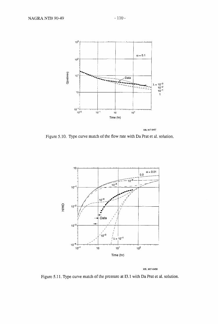
NAGRA NTB 90-49
102
C :§ 101
E 0
10
- 110-
I
I
I
~- I I
.~~ I ~-,.,-,--I - ..... "'-"'-"-:: i
10
Time (hr)
(0= 0.1
.. ~ '::"~=-.::.:...:.=-
A. = 10-3
10-2
10-1
1
XBL 907·6457
Figure 5.10. Type curve match of the flow rate with Da Prat et aI. solution.
o I I
/-"" ,......'i' /' /
/'/' ,
(0= 0.01 0.0
1 0-4 .~~ -- ./ /fit
10-2 f-:f--;L-----t----.... -"....;t-... --t---'-rl-:' ___ +-___ --J • I; ..
.. II ;'
-. ··Data / / I
10-3+-------t---~-,_r------+----~
I
/10-3 I
I A. = 10-1 I
10~+_-,-r~~r-~~~~-~~~~-._.~~
10-1 10
Time (hr)
XBL 907·6458
Figure 5.11. Type curve match of the pressure at 13.1 with Da Prat et al. solution.

NAGRA NTB 90-49 - 111 -
_ Ko [[ (Sso Op) 112 + p] 112 . r] h - --'-"----------
- pKo [[(SsOOP)I12 + p] 112] (5.4)
and the dimensionless flow rate at the well is simply:
_ [(S,Dlip)\12 + pj\12. K\ [[(S'DIiP)\12 + pj\12]
'lD-- pKo [[(SsOOP)I12 + p] 112]
(5.5)
where SsD is the ratio of the fracture speci fic storage to that of the matrix, Ko is the ratio of the
hydraulic conductivity of the same, and 0 = Kolbb. where bo is the ratio of fracture thickness to
the well radius. Equations (5.4) and (5.5) are evaluated for various values of 0 and plotted in Fig-
ures 5.12 and 5.13. Also plotted are the observed data. As can be seen in Figure 5.12, the match
with the interference data at 13.1 is now much better compared to the case of Da Prat's solution.
However, the late time data of 13.1 is still not matched very well. Also, the observed flow rate
curve is much flatter in the late time than the theoretical curves (Figure 5.13).
Nonetheless. the concept of leakage seems to explain the trend of the data: low interference
pressure, and the flattening of the flow rate curve. The weak hydrologic connection between
Interval 11.2 and 12.2 may be through this low permeability rock matrix. It is worth noting that
the 1988 seismic tomography results indicate the existence of a feature (B) that extends diago-
nally from the access tunnel toward B087.001 (Figure 4.9). This may be the actual conduit of
the leaking water. Although a localized leakage cannot be handled with an analytical solution,
this will also explain the low pressure at 13.1 and the flattening of the flow rate curve.
5.4.4. Boundary Effect
In the previous analyses the boundary effects of the tunnels were neglected. However, dur-
ing the injection test it was observed that water was seeping out thorough the shot-crete along the
zone where the FRI fracture intersects the access drift (peterson, personal communication 1989).
In this section the effects of the drifts on the measured pressure is investigated. Because of the
complexity of the geometry and the boundary conditions, a numerical model was used, where the
FRI fracture is assumed to consist of a two-dimensional interconnected channel network (Figure

NAGRA NTB 90-49
o I I
- 112 -
S = 1.0 So
1O-3 _l__--II-..,...;...t.J...::....,Lt-----+-----+--------1
10~-l---4~~~-~~~m-~~~~+--~~~~
10-1 10
Time (hr)
XBL 907-6459
Figure 5.12. Type curve match at 13.1 with a leaky fracture zone solution.
~ o u::
1O-1-+------+-----t-----+___----i
10-2 -+-----r----.-...-.,..-,~-....,__...--r-T""TTrr+____,.___r..--rT"TT"T+____.__,__,r-r--r_rrrl
10-2 10
Time
XBL 907-6463
Figure 5.13. Type curve match at Il.2 with a leaky fracture zone solution.
NAGRA NTB 90-49 - 113 -
5.14). Both models were assumed to be initially at steady-state subjected to the same hydrostatic
head. Then the node that corresponds to the location where the intetval 11.2 intersects the frac
ture was opened to simulate the field test. Results of the simulated well test are compared using
the cases with and without tunnels. Figure 5.15 shows the comparison of the pressures at 13.1.
As can be seen from the figure, the effect of the tunnels is felt at time equals 10. The curve for
the case with the tunnels flattens and deviates compared to the case without the tunnels, as the
pressure in 13.1 responds to the atmospheric pressure in the laboratory tunnel. However, the
actual data shows no sign of flattening as can also be seen in the figure. The effect of the labora
tory tunnel on the interference data at 13.1 seems to have been minimal. This indicates that the
permeability of the fracture around the laboratory tunnel is low. This agrees with the obsetvation
(peterson, personal communication 1989) that no apparent increase of water seepage was noted
in the vicinity where the FRl fracture intersects the laboratory tunnel.
Figure 5.16 shows the comparisons between the flowrates at 11.2 for the two cases. The
figure shows that the effect of the tunnels would be seen as a flattening of the flowrate decline
curve. However, it is not as significant as the previous case. The inflection in the actual data
cannot be explained by the effect of the tunnels alone.
5.5. Conclusions
The hydraulic tests have confinned the hydrologic significance of the fracture zone which
was previously identified by the seismic tomography. It appears that the majority of the flow
occurred within the relatively thin fracture zone which connects Interval 11.2 and 13.1. A weak
but definite hydrologic connection between Intetval 11.2 and 12.2 was also observed. Feature B
identified by the seismic tomography that extends diagonally from the access tunnel to
BOFR87.001 may partially explain this hydrologic connection.
Because of the anomalous interference and flow-rate data, four different scenarios that
differ from the ideal conditions were examined. They are 1) skin, 2) anisotropy, 3) leakage, and
4) boundary effects. Although it is possible for all of the four conditions to coexist, the most
plausible scenario seems to be the leakage effect outside of the fracture plane.

NAGRA NTB 90-49
E L{) -.;t
~I.f------ 45 m
- 114 -
13.1 /
11.2
XBL 907-6460
Laboratory tunnel
Access tunnel
Figure 5.14. Numerical model of the FRI fracture a) with and b) without tunnels.

NAGRA NTB 90-49 - 115 -
3: o u:
• + • ...
f
•
• 10
• +
•
t
dOd bl5otiotO+00·060
0<) f- •••••••••• ~o.£) •••••
0 •• • ,,:. ~.
+ No tunnels o Access tunnel only * Both tunnels
XBL 907-6461
Figure 5.15. Simulated data for the pressures at I3.1.
,
+ Simulation 0 Simulation without tunnels
* Simulation with tunnels
10-4
~ ..... ....... .............. ....... _ ..... .... ~ .,.-10-6
XBL 907-6462
Figure 5.16. Simulated data for the flow rates at n.2.

NAGRA NTB 90-49 - 117 -
6.0. INFLATION TESTS
6.1. Introduction
The putpOse of the inflation tests was to determine the mechanical stiffhess of the kakirite
fracture intersected by BOFR 87.001 and BOFR 87.003 in order to evaluate the influence of
changing fluid pressure in this fracture on seismic waves propagation and hydrologic behavior.
The mechanical stiffhess of the kakirite fracture in the FRI was pertinent to interpretation of both
the in-situ hydrologic and seismic experiments. Relative to the hydrologic measurements, stora
tivity of a fracture is directly related to fracture stiffhess. In addition, the fracture stiffhess relates
the applied stress to the changes in fracture aperture which significantly affects the permeability
of the fractures. With respect to the seismic measurements, the objective was to obtain an in-situ
measurement of fracture stiffhess which could be input into the theoretical model to predict the
effect of the fracture on seismic wave propagation. If changes in fluid pressure were sufficient to
change the fracture stiffhess, then the effects of this change would be observed in seismic meas
urements made during the inflation tests.
6.2. Description of the Experiment
In order to determine the stifIhess of the fracture it was first necessary to measure the defor
mation of the fracture in response to a change in stress across the fracture plane. The change in
stress was provided by pressurizing an interval between two packers. In order to perfOtm defor
mation measurements while at the same time pressurizing the fracture, special equipment, the
Bofex, which is schematically illustrated in Figure 6.1 was required. This figure shows that the
displacement measurements were made between two anchors fixed in the borehole. The linkage
between the anchors passes through the mandrel of the packers, so the anchors are independent
of packer deformations caused by water pressure changes. The displacement transducer is
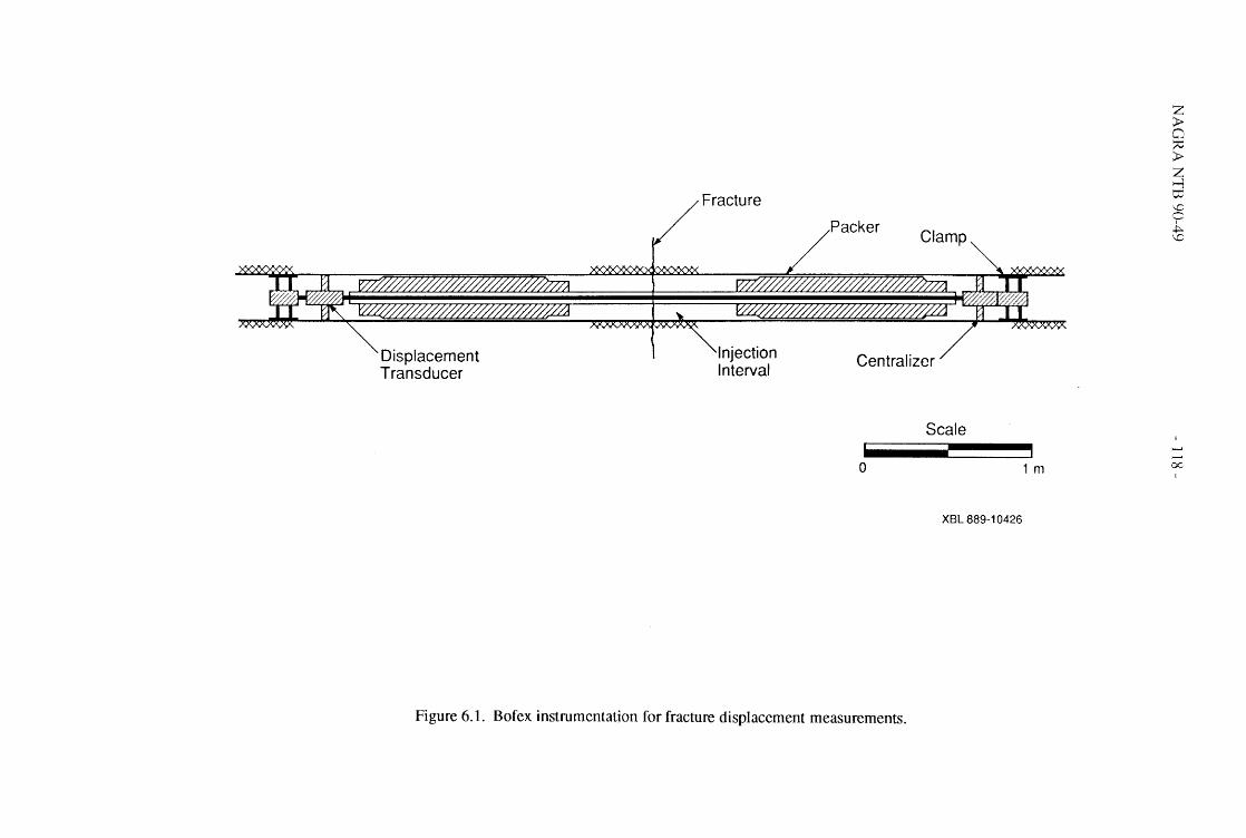
Fracture
Packer Clamp
Displacement Transducer
Injection Interval
Centralizer
Scale
o
XBL 889-10426
Figure 6.1. Bofex instrumentation for fracture displacement measurements.
1 m
z » o ~ » z ..., ttl '-C C
I
+:\.C
oc

NAGRA NTB 90-49 - 119 -
rigidly attached to one anchor (clamp at right in Figure 6.1). A spring-loaded plunger in the
transducer rests against the other anchor (at left in Figure 6.1) The output of the displacement
transducer was ± 10.0 V for a total possible displacement of ±6.35 mm (0.25 in). The electronics
provided a 1 mV sensitivity, so the displacement resolution was 0.64 J..Un.
As discussed in Chapter 5, interval 11.2, which contained the kakirite fracture was about 4
m long (Figure 5.3). This interval encompassed several fractures. Inspections of the core from
BOFR 87.001 and BOFR 87.003 suggested, however, that the kakirite fracture (which actually
consisted of two closely spaced fractures in the core from BOFR 87.(01) was the principal con
ductor. For the inflation tests, interval 11.2 was therefore shortened considerably and centered
over the kakirite fractures. Packer locations are shown in Figure 6.2 and tabulated in Table 6.1.
Similarly, new packer locations were determined for BOFR 87.003.
BOFR 87.001 and BOFR 87.002 were filled with water by placing packers in the end of the
holes as shown in Figure 6.2. Packer P1.1 was a special design with a seal so that the push rod
for the seismic transducer could pass through the packer while keeping water in the borehole.
Packers P1.2 and P1.3 were inflated simultaneously after the hole was filled with water.
Packer P3.1 was inflated in BOFR 87.003 first. Then the borehole was filled with water and
packer P3.2 was inflated. This procedure assured that no air was in the injection intervals 11.2
and 13.1. Packers in BOAU 83.034 and BOFR 87.004 were not disturbed. Therefore, for the
inflation test, water pressures were monitored in intervals 11.2,13.1,134.1 and 14.1.
In order to accommodate the seismic measurements, pressure and flow tubes to interval 11.2
were routed up BOFR 87.001 to the access tunnel, back through another borehole to the labora
tory tunnel and then to the monitoring apparatus, a distance of about 150 m. Packers P1.2 and
P1.3 were inflated to about 50 bars and P3.1 and P3.2 were inflated to about 30 bars. When pack
ers P1.2 and P1.3 were inflated the pressure in 11.2 increased to 15 bars and a slight reaction was
noted in 13.1. The 15 bar pressure was held only momentarily. Interval pressure in 11.2 and 13.1
were left to stabilize overnight at about 1.5 bars.

NAGRA NTB 90-49
....-o o r---:
- 120 -
N o o
co o 0) Upper Access Tunnel
r---: co o m
Tr+
Kakirite)4+ Fracture
P1.2
R1
P1.3
11.2, Bot 1
Lower Laboratory Tunnel
Scale
o 5m
I8l Bofex Anchor Point _ Hydraulic Packer
• Mechanical Packer
® R1• R 2 Receiver Locations
® T1 • T2 Transmitter Locations
o ..;t ('I') ('I') o 0 M M co co o 0 0) 0)
B087.004
T1
XBL 889·10429
Figure 6.2. Plan view showing instrumentation locations for inflation test.

NAGRA NTB 90-49 - 121 -
Table 6.1. Packer and interval locations for inflation tests
Hole Packer Interval Location in Borehole (m)
BOFR 87.003 P1.1 0.0 - 1.0 P1.2 8.6 - 9.6 P1.3 11.1-12.1
11.2 9.6-11.1
BOFR 87.003 P3.1 1.7 - 2.7 P3.2 4.2 - 5.2
13.1 2.7 - 4.2
The seismic receiver location was fixed in BOFR 87.001 at the position shown in Figure
6.2. A set of seismic measurements were obtained with the transmitter at 0.5 m intervals over the
length of BOFR 87.002. The transmitter location was then fixed as shown in Figure 6.2 so that
the direct ray path between receiver and transmitter was roughly normal to the fracture zone.
The Bofex 1 transducer required several hours to stabilize. It also generated a 8kHz signal
which was detected by the receiver in borehole BOFR 87.001. Thus, when seismic measure-
ments were made it was necessary to disconnect power to the transducer. Stabilization after
reconnection occurred in a matter of minutes.
Measurements associated with the inflation tests took place over the course of six days. A
time line of events and pressure history of 11.2 and 13.1 are shown in Figure 6.3. On the first day
interval 11.2 was pressurized to 20 bars and maintained constant. Flow rates were measured as a
check on hydrologic properties measured in the previous test. Seismic Ineasurements were made
periodically with the receiver and transmitter in fixed locations.
At about 17 hours into the experiment the pressure in 11.2 dropped to 6 bars for about 3
hours due to. equipment problems. Additional seismic measurements were made and then the
interval pressure was increased from 6 to 35 bars and held at that level for about 9 hours. Defor-
mation and pressures were monitored and periodic seismic measurements were made during this
time. Due to further equipment problems it was necessary to reduce the Il.2 pressure to 20 bars
after this 9-hour duration.

NAGRA NTB 90-49 - 122 -
Pressurize I1.2 to 20 bars Seismic crosshole measurements
I1.2 I1.2 and 13.1 pressurized rt pressure to 0 .l I1.2 and 13.1 pressure to 0
Time Line 0 ~1 .. ---~-----L-.. -':'-L..oI!!~-----L<!!!:.------------l120 hr
~ Periodic Seismic, Continuous Displacement Measurements
36 ,..-. BOFR 87.001
27
,A.
l
9 V
o 24~-----------------------.
18
'§' C'O 8-0> 12 :s CJ) CJ) 0> c:
6
BOFR 87.003
-o ~-------_____________ L-_______________ ~
o 30 60
Time (hours)
90 120
XBL 907-2581
Figure 6.3. Time line of events in inflation test and pressure history in intervals 11.2 of BOFR 87.001 and 13.1 ofBOFR 87.003.

NAGRA NTB 90-49 - 123 -
At about 40 hours a set of seismic measurements were made with the transmitter at 0.5 m
intervals along the length of BOFR 87.002. An additional set of seismic measurements were
then made with the receiver moved to a distance of 4.69 m in borehole BOFR 87.001 and the
transmitter at 0.5 m intervals along the length ofBOFR 87.002.
At about 45 hours the experimental configuration was changed. In order to further inflate
the fracture, interval 13.1 was pressurized to 20 bars while maintaining 20 bars pressure in inter
val n.2. Before the next phase of the test was carried out, the seismic transducer locations were
changed so that both source and receiver were in close proximity to the fracture. As shown in
Figure 6.2 the receiver was placed in BOAU 83.030 at approximately 2 m in the hole while the
transmitter in BOFR 87.002 was relocated so that the direct line ray path between the transducers
was normal to the fracture zone.
In order to remove the receiver from BOFR 87.001 it was necessary to drain the borehole.
It was then refilled, but this process caused a large perturbation in the Bofex 1 readings. Due to
schedule constraints it was necessary to begin injection into interval 13.1 before Bofex 1 was res
tabilized.
A set of seismic measurements were made before interval 13.1 was pressured. It was then
pressurized to 20 bars. Pressures and flow measurements were made at short time intervals dur
ing the initial pressurization. In order to permit independent inflation of the packers in BOFR
87.003, the pressure line was used as a packer inflation line. Thus, for the inflation test, both flow
and pressure measurements were made on the same line. In addition, the flow line from 11.2 had
been connected to the flow line from 13.1, so the total flow was the sum of that going to both
intervals.
Seismic measurements were made just prior to releasing the pressure to zero in intervals
11.2 an 13.1 at about 62 hours. Displacements were monitored and periodic seismic measure
ments were made until the equipment was removed at 120 hours.
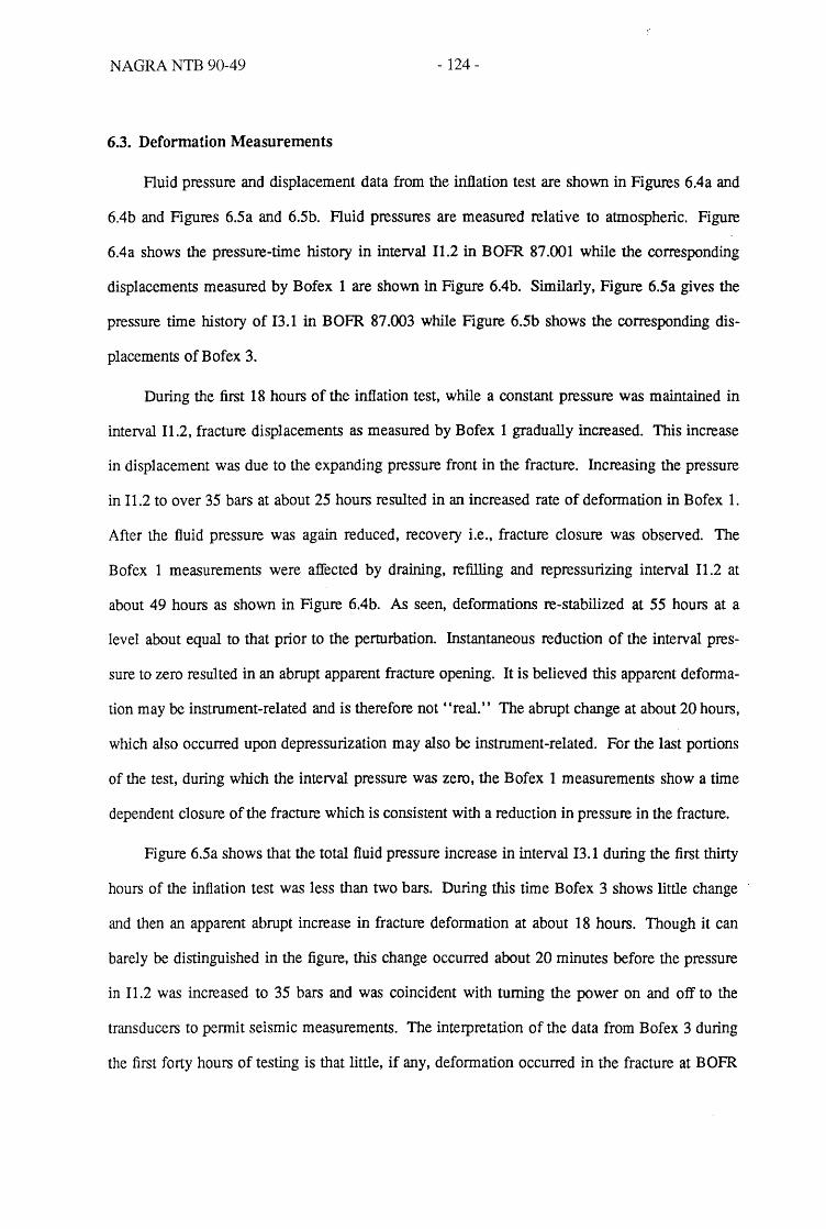
NAGRA NTB 90-49 - 124-
6.3. Deformation Measurements
Fluid pressure and displacement data from the inflation test are shown in Figures 6.4a and
6.4b and Figures 6.5a and 6.5b. Fluid pressures are measured relative to atmospheric. Figure
6.4a shows the pressure-time history in interval 11.2 in BOFR 87.001 while the corresponding
displacements measured by Bofex 1 are shown in Figure 6.4b. Similarly, Figure 6.5a gives the
pressure time history of 13.1 in BOFR 87.003 while Figure 6.5b shows the corresponding dis
placements of Bofex 3.
During the first 18 hours of the inflation test, while a constant pressure was maintained in
interval 11.2, fracture displacements as measured by Bofex 1 gradually increased. This increase
in displacement was due to the expanding pressure front in the fracture. Increasing the pressure
in 11.2 to over 35 bars at about 25 hours resulted in an increased rate of deformation in Bofex 1.
After the fluid pressure was again reduced, recovery Le., fracture closure was observed. The
Bofex 1 measurements were affected by draining, refilling and repressurizing interval 11.2 at
about 49 hours as shown in Figure 6.4b. As seen, deformations re-stabilized at 55 hours at a
level about equal to that prior to the perturbation. Instantaneous reduction of the interval pres
sure to zero resulted in an abrupt apparent fracture opening. It is believed this apparent deforma
tion may be instrument-related and is therefore not' 'real." The abrupt change at about 20 hours,
which also occurred upon depressurization may also be instrument-related. For the last portions
of the test, during which the interval pressure was zero, the Bofex 1 measurements show a time
dependent closure of the fracture which is consistent with a reduction in pressure in the fracture.
Figure 6.5a shows that the total fluid pressure increase in interval 13.1 during the first thirty
hours of the inflation test was less than two bars. During this time Bofex 3 shows little change
and then an apparent abrupt increase in fracture deformation at about 18 hours. Though it can
barely be distinguished in the figure, this change occurred about 20 minutes before the pressure
in 11.2 was increased to 35 bars and was coincident with turning the power on and off to the
transducers to permit seismic measurements. The interpretation of the data from Bofex 3 during
the first forty hours of testing is that little, if any, deformation occurred in the fracture at BOFR
NAGRA NTB 90-49 - 125 -
36 "....... SOFR 87.001
27
I .A.- I
1 I I I I I
~ I I 9 I I I I
I I o I
14~------~--r-------~------~------------------~
12 __ 10
~ 8
Q)0'l :S.£ ufE ~c..
C 61 LLO
Q)
E 4 Q) u C\l 0.. (/)
:.0 Q) !o-:::)
t5 C\l u:
2
0
-2
-4
-6
-8
-10
* ~Q) :::J .... _:::J UC/l ceo Ltu
0 30
...... E----- Restabilization
60
Time (hours)
90
Sofex 1
120
XBL 907-2584
Figure 6.4. (a) Pressure history in interval 11.2, BOFR 87.001, during inflation test; (b) fracture displacements as measured by Bofex 1 in BOFR 87.001 during inflation test. Vertical dashed lines show coincidence in time of events.

NAGRA NTB 90-49 - 126 -
36
SOFR 87.003
27
en Co e ~ 18 :J CJ) CJ) Q) ~ a..
9
I-- I
0 I
I
24
22
20
18
-10 ~----------------------------------------------~ o 30 60
Time (hours)
90 120
XBL 907-2585
Figure 6.5. (a) Pressure history in interval 13.1, BOFR 87.003, during inflation test; (b) fracture displacements as measured by Bofex 3 in BOFR 87.003 during inflation test. Vertical dashed lines show coincidence in time of events.

NAGRA NTB 90-49 - 127 -
87.003 in response to the pressurization of Il.2. When interval 13.1 in BOFR 87.003 was pressur
ized, the fracture opened rapidly in response to the pressure front moving out from the borehole.
The resulting total deformation was greater than observed for Bofex 1 for a similar duration of
time. This observation is consistent with the data showing flow rates to be higher at the same
injection pressure in 13.1 than in 11.2. Since the fracture intersected the tunnel wall at an oblique
angle, the stress notmal to the fracture at locations in close proximity to the wall, such as in
BOFR 87.003, was less than at other locations deeper in the rock mass. This lower nonnal stress
could lead to higher fracture permeability. In addition the wedge of rock formed at the intersec
tion of the fracture plane and the tunnel wall may have been deformed, resulting in further open
ing of the fracture.
After depressurization of 13.1, Bofex 3 showed a time dependent closure in response to
pressure reduction in the fracture. This response was similar in form, though greater in magni
tude than observed in Bofex 1 (Figure 6.4b).
6.4. Analysis of Deformation Measurements
The deformation measurements were made in order to evaluate the mechanical stifihess, at
an in-situ scale, of the kakirite fracture. The analyses were complicated by the fact that the fluid
pressure in the fracture was localized in extent. Therefore, in addition to the usual calculation of
stiflhess, referred to as a zero-order approximation, two additional calculations were performed
to evaluate the effects of the limited areal extent of the fluid pressure. The first modelled the frac
ture as a single crack with stifihess. The second modelled the fracture as a co-planar array of
parallel cracks.
The stifihess, le, of a fracture is defined as the ratio of the applied stress to the deformation
it produces. The units of 1C are Palm. The deformations are those which occur in addition to the
deformation of the intact rock adjacent to the fracture. As a zero-order approximation, then, the
measured values of displacement of the fracture in FR.I can be used directly to calculate fracture
stiffuess. Using the measured value of displacement from Bofex 1 after 17 hours, assuming a
pressure increase of 19 bars and correcting only for the angle between the Bofex and the normal

NAGRA NTB 90-49 - 128 -
to the fracture, 1C is given by:
1C = 1: = 1.9 X 10⁶
Pa = 1.3 x 10¹² Palm () 1.4 x 10⁻⁶ m
(6.1)
where P is pressure and () is displacement.
The assumption implicit in this calculation is that the pressure was everywhere equal and
applied over a fracture area of very large extent. Since the fluid pressure was non-unifonn and of
limited extent in area, the calculation in Equation (6.1) ~hould yield a very conservative (high)
estimate of stiffhess.
A more realistic model is shown in Figure 6.6, element I (top of figure). The fracture is
represented as a single two-dimensional mathematical crack in plane strain, with a spatially vary-
ing pressure applied over a portion of the crack surface. The effect of the fracture stiffuess is
represented schematically in the figure by springs of stiffuess 1C connecting the surfaces of the
crack. Using field data as input to the model, values of 1C as a function of crack length, 2c, were
determined.
The approach to solving the problem analytically involved the use of linear elastic fracture
mechanics. Since elasticity was assumed, the problem in I (Figure 6.5) could be decomposed
into two simpler elements designated by II and III in the figure. By supetpOsition, then:
(6.2)
where ()(x) is the displacement in the y direction. The value of ()ZO) was known from the Bofex 1
measurements.
The pressure distribution, P, in the crack was represented by a cubic polynomial of the
form:
(6.3)
where
P I x=o = constant = Po

NAGRA NTB 90-49 - 129-
II
+ Fracture Stiffness K
XBL 901-113
Figure 6.6. Modelling the inflation experiment by a pressurized crack with stiffhess. Assuming elasticity, model I is decomposed into two simple models designated II and III.

NAGRA NTB 90-49 - 130-
For the FR.I test coefficients in (6.3) were evaluated as:
ao = 1 a2 = 0 3 1 (6.3a)
a 1 = - 2t a3 = 2P
Calculations were carried out assuming pressure conditions after 17 hours were represented by
Po = 19 bars at x = 0 and the pressure in BOFR. 87.003 was 1.87 bars. Assuming the distance
between pressure measurement points, as measured along the fracture, was 10 m, the value of 1 =
13.6m.
To calculate displacements it was necessary to obtain expressions for the mode I stress
intensity factor, K1. For an elliptical crack of length 2c and point loads of magnitude P located at
a distance x = ± b from the midpoint of the crack, KI is given by:
(6.4)
The stress intensity factor for a distributed pressure is found by integration of Equation
(6.4) over the length of the crack. Substitution of Equation (6.3) into (6.4) and integration yields:
II c . -1.1 2.. _1 .k [ 1
1/2 { [ 211n
KI = 2 -; Po sm ( c ) + 21 c 1 - c2 - 21
+£ [_ [1_Ll1/2 +1.(1_.L)3n+~]} 2z3 c2 3 c2 3
(6.5)
The displacements, B&), corresponding to the unconstrained crack (element IT in Figure.
6.6) can now be found. Substitution of Equation (6.8) into the following equation yields dis-
placements perpendicular to the crack plane as a function of position x:
(6.6)
Displacements from (6.6) with the pressure distribution given by (6.3) and (6.3a), a Young's
modulus, E, of 42.7 GPa and a Poisson's ratio of v = 0.25 are given in Figure 6.7 for a range of

NAGRA NTB 90-49 - 131 -
0.0004 (a)
..-.. E ---- 0.0003
+-' c Q)
E 0.0002 Q) C,,) CO c.. C/) 0.0001 0 C = 20
0 0 20 40 60 80 100
Distance (m) 0.0004
(b) ..-.. E --- 0.0003 +-' c Q)
E Q) 0.0002 () CO c..
.C/) 0.0001 0
0 0 200 400 600 800 1000
Distance (m) XCG 899-4695
Figure 6.7. Displacement as a function of distance from the midpoint of the crack in element II, assuming 1= 13.62 m and crack lengths from 20 to 1000 m.
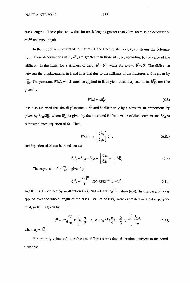
NAGRA NTB 90-49 - 132 -
crack lengths. These plots show that for crack lengths greater than 20 m, there is no dependence
of Oil on crack length.
In the model as represented in Figure 6.6 the fracture stifihess, 1(, constrains the deforma
tion. These deformations in IT, SIT, are greater than those of I, 01, according to the value of the
stiffhess. In the limit, for a stifihess of zero, S1 = oIT, while for 1C~oo, S1~O. The difference
between the displacements in I and IT is that due to the stiflhess of the fractures and is given by
o~). The pressure, P'(x), which must be applied in ITI to yield these displacements, Sti), must be
given by:
P'(x) = KOtx) (6.8)
It is also assumed that the displacements oIT and 01 differ only by a constant of proportionality
given by o~x)lofo) where o~O) is given by the measured Bofex 1 value of displacement and ofa) is
calculated from Equation (6.6). Thus,
(6.8a)
and Equation (6.2) can be rewritten as:
~ill _ ~r ~IT - [o~O) _ 1] ~IT U(x) - U(x) - U(x) - ~IT U(x)
U(O) (6.9)
The expression for o~) is given by
ill 2Kpr In" O(x) = E [2(c-x)/1tJ (1- v~) (6.10)
and KF is determined by substitution P'(x) and integrating Equation (6.4). In this case, P'(x) is
applied over the whole length of the crack. Values of P'(x) were expressed as a cubic polyno
mial, so KF is given by
(6.11)
where ao = o~)
For arbitrary values of c the fracture stifihess K was then determined subject to the condi-
tions that

NAGRA NTB 90-49 - 133 -
(6.12)
where ()to) is, again, the measured displacement. Thus, combining Equations (6.10) and (6.11)
with (6.9),
~I 4c (l-V)2 _ r: I ()~O) [ 1t U(O) -ao = - ...... _ ..... - -v2 lC-- ao - + al c+ 1t E ao 2
Hz cZ
: + ~ a3 c3]} (6.13)
For different values of crack length it is then possible to determine the corresponding stiflhess.
These are plotted in Figure 6.8. While the extent of the fractured zone is not known, it is
expected to be in excess of ten times the pressurized region. For crack lengths of this order of
magnitude Equation (6.13) yields values of lC on the order of 4 x 10¹⁰_2 X 1011 Palm, or almost
two orders of magnitude less than that derived for two half-spaces joined by a stiflhess as in
Equations (6. 1).
In the approach just described the displacements along the face of the crack are given as a
function of the stress intensity factor. Because of the simplifying assumptions used in deriving
the stress intensity factor, there is a discrepancy between displacements predicted using it and
those which would be predicted by a full elasticity solution. This discrepancy is very small close
to the crack tip but increases with distance from the work tip. The result of the approximations
involved in using a stress intensity factor to calculate the stiflhess of a crack with springs is that
the calculated stiffness is lower than would be predicted by the full elastic solution.
A second approach involving a different set of assumptions was to model the kakirite frac-
ture as a row of two-dimensional coplanar cracks of equal crack length, 2c, and unifonn spacing,
2b. In this model the ligaments of material between the cracks can be taken to represent the
areas of contact between the faces of the fracture, and the cracks to represent those areas not in
contact.
Simulations of the model for different crack spacings 2b and ratios of crack length to cra~k
spacing c/b were conducted assuming the material properties already noted above in the

NAGRA NTB 90-49 - 134-
20.0.1° .......... ---.,,-------------------,
o~--~--~---~---~---~-~ o 200 400 600 800 1000 1200
Crack length (m) XCG 899-4694
Figure 6.8. Predicted fracture stiffuess as a function of crack length.

NAGRA NTB 90-49 - 135 -
TWODD two-dimensional boundary element program developed by Crouch and Starfield (1983).
Crack spacing, 2b, ranged from 50 m as upper limit to 0.10 m as the lower limit. Crack length to
crack spacing ratios, c/b, ranged from 0.05 to 0.99. The range of c/b values for each b was
selected to best match observed results. The deformations were calculated for a position of 0.75
m above the midpoint of the center fracture.
The number of cracks for each simulation was chosen to accommodate the extent of the
pressure distribution as observed in the field so that the row of cracks extended from x = 0 m to x
= ±13.6 m with the first crack centered at the origin. The pressure distribution was assumed to
act only within the cracks. The effect of additional unpressurized cracks was found to be
minimal. Simulations were run for a single crack of 40 m length containing the entire pressure
distribution and c/b = 0.8. Additional deformation for fourteen cracks on either side of the pres
surized crack increased the deformation by less than six percent. Simulations for a smaller crack
spacing of 2b = 2 m and a c/b ranging from 0.95-0.99 showed an even less pronounced effect on
the deformation.
Simulations were run for crack spacing values ranging from 2b = 0.1 m to 2b = 1,0 m, for a
range of c/b values from 0.05-0.99. Results for the simulation are shown in Figure 6.9. All
simulations show the same trend of deformation increasing exponentially with increasing c/b, or
decreasing contact area. The effect of the crack spacing 2b on the deformation is significant; for
a given c/b, the deformation increases exponentially with increasing b, Proportional decrease in
c/b for a given deformation is less than the proportional increase in b. If Figure 6.9 is interpreted
in terms of contact area, it shows that for a given contact area deformation increases with
increasing b, and the contact area required to provide a given deformation increases with increas
ing b. This corroborates the work of Hopkins et al. (1987), who found that for a given contact
area, the smaller the individual areas of contact the higher the stiflhess of a fracture.
The horizontal line in Figure 6.9 represents the measured deformation in situ
(1.42 x 10⁻⁶ m). It is seen that for a given crack size quite large spacings are required to match
the observed results. Figure 6.10 is a plot of the percent contact area (1 - c/b) required to match

NAGRA NTB 90-49 - 136 -
20~----~-----.-----.------,-----,-----~
- 15 to o
>-::::l 10 C o ~ E o ~ 5
b= 0.1 m
OL-____ ~ ____ ~ ____ ~ ______ ~ ____ ~ ____ ~ o 0.1 0.2 0.3 0.4 0.5 0.6
c/b XCG 901-4508
Figure 6.9. Deformation between two points located 0.75 m either side of the midpoint of the center crack of a row of pressurized coplanar cracks.
0.8
0.7 f- -
~ ~ ctl
0.6 ell f- -Co U ctl C 0.5 0 f-! -u "C ell
.!::! "ffi 0.4 7-E
-
0 Z
0.3 ~ -
0.2 I I I 1 I 0 0.1 0.2 0.3
b (m)
XCG 901-4507
Figure 6.10. Normalized contact area of fracture faces as a function of crack half spacing b for a deformation of 1.42 x 10--6m.

NAGRA NTB 90-49 - 137 -
the observed infonnation as a function of crack spacing. This shows that for spacing 2b of 0.1 m
the contact area would still have to be about 66 percent. Because of limitations in computing
capacity it was not possible to make calculations of deformation for b less than 0.05 m. An
extrapolation of the curve in Figure 6.1 a (dotted line), based on a curve fit of the values obtained
at larger values of b shows that even if the crack spacing 2b were 0.05 m, the contact area would
be about 59 percent.
An independent assessment of the contact area in the fracture zone could not be made.
However, since the zone contained gouge material, high contact areas might be expected.
Another possibility is that the fluid in the fracture was confined to channels and did not have
access to all available void space.
For a row of co-planar cracks the average displacement, 0 is given by
0= -8ab(l-y2)[ln cos(1tc!2b)) 1tE
Since by definition, stiffness, K, is related to 0 by
then the stiffhess of a row of co-planar cracks is given by:
1 -8b(l-y2)[ln cos(1tc!2b)] K - 1tE
(6.14)
(6.15)
(6.16)
Using equation 6.16 and values ofc and b from Figure 6.9 corresponding to the in-situ measured
deformation, values of K were calculated which ranged from 2 x lOll Palm to 3 x lOll Pa/m. As
expected, these correspond to the high end of the range of stiffness values obtained from the
crack-with-springs model.
The effect of a single fracture with a stiffuess of 3 x 10¹¹ Palm on seismic wave propagation
can be evaluated using the seismic displacement discontinuity model described in the initial part
of this section. Figure 6.11 is a plot of the magnitude of the transmission coefficient, ITI, and nor-
malized group time delay, tg/tgo' for a wave nonnally incident upon a fracture (Pyrak-Nolte et al.,
1990). Values of [co/(K1z)] were calculated for K = 3 X lOll Pa/m, z = 1.4 X 10⁷ kg/m2s, and co
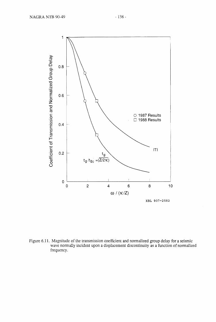
NAGRA NTB 90-49 - 138 -
>. ~ Q)
0 0.8 Q.. :::::l 0 lo...
CJ "'0 Q)
.~ ~
E 0.6 lo...
0 Z "'0 C ~
C o 1987 Results 0 o 1988 Results 'en C/)
0.4 'E C/)
c ~ lo...
~ -0 --c ITI Q)
'0 0.2 tg ;,;::: - tg Itgo =(Zl2K) Q) 0 ()
o o 2 4 6 8 10
0) I (K/Z)
XBL 907-2582
Figure 6.11. Magnitude of the transmission coefficient and normalized group delay for a seismic wave nonnally incident upon a displacement discontinuity as a function ofnonnalized frequency.

NAGRA NTB 90-49 - 139 -
corresponding to the center frequency of the P-waves in the tomographic survey. For the 1987
survey this frequency was about 6 kHz while for the 1988 survey it was about 10 kHz. In Figure
6.11 the corresponding values of ITI and tg/tgo are plotted as circles for the 1987 survey and
squares for the 1988 survey.
For a 6 kHz wave normally incident on a fracture with stiffuess of 3 x 10¹¹ Palm the value
of ITI is seen to be about 0.75 while for a 10 kHz wave it is about 0.56. A value of ITI = 0.75
means that, a wave propagated across the fracture would have an amplitude about 25% lower
than one propagating over the same path length of intact rock. Because of the higher frequency
used in the 1988 survey, the amplitude reduction (Le. ITI = .56) is predicted to be greater. From.
Figure 6.11 it is seen that the value of tg/tgo for the 1987 survey was about 0.55 while for the
1988 survey it was about 0.31. Since tgo = [1/2 (K"/z)], values oftg were found to be 0.013 m sec
and 0.007 m sec for the 1987 and 1988 surveys, respectively. A value of 0.013 m sec means that
the measured travel time of a wave crossing the fracture would be 0.013 m sec longer than that of
a wave propagated over the same distance through intact rock. These results indicate that,
because of the difference in frequency of the sources used in the two surveys, the fracture zone
would be less distinct in the 1988 tomogram than in the 1987 tomogram, and this was observed.
If the group time delay for the 10 kHz waves is converted to an effective change in velocity, the
theory predicts that the fracture zone should result in about a 1 % decrease in velocity relative to
, 'unfractured" rock. This decrease is also similar to the difference between background and frac
ture zone velocity in the tomogram after anisotropy was removed.
In order to complement the in-situ stiffuess measurements, laboratory measurements were
made on fractured specimen #2 (see Chapter 3), containing a single natural fracture. The meas- .
urements were performed in conjunction with the seismic measurements under saturated condi
tions. The apparatus used to jacket the specimen are described in Chapter 3.4. Additional
apparatus consisted of a capillary tube, partially filled with water under 10 psi pressure, con
nected to the saturated specimen. As axial load on the specimen was increased water was
expelled from the fracture. Upon unloading water flowed into the fracture. Assuming water

NAGRA NTB 90-49 - 140-
moved into or out of only the voids in the fracture, the stiffuess of the fracture is given by
lC = (J/(flv/A)
where (J is the normal stress on the fracture, flv is the change in volume of water and A is the
fracture area.
Five repeat measurements were made on fractured specimen #2. Typical results are shown
in Figure 6.12a,b. Shown in part a of the figure is the water volume change as a function of
applied stress. Arrows indicate the sequence of loading steps. As load increased the volume of
water in the capillary tube increased, indicating expulsion of water from the specimen. Upon
unloading water moved back into the specimen. However as can be seen, there was a large hys
teresis in the measurements; more water was expelled than imbibed. It is believed that the meas
urements reflect the movement of water in and out of the porosity of the intact rock as well as the
fracture. The highly foliated nature of the rock apparently introduces more interconnected poros
ity than is usually observed in granite. Loading the rock to the highest load level also may have
introduced some dilation, leading to the observed decrease in water volume at the highest load
ing step.
Fracture stiffuess values calculated from the volume change measurements are shown in
Figure 6.12b. These are incremental values, calculated from the volume change at each load
step. Because of the affect of the porosity of the rock adjacent to the fracture, these stiffuess
values are lower than the true fracture stiffuess; it is thought that the error is less for the values
obtained during unloading. The laboratory measured values of stiffuess (during unloading) were
about an order of magnitude higher than those measured in-situ. If the in-situ value of fracture
stiffi1ess was comparable to that of the laboratory measurements, the seismic displacement
discontinuity theory predicts that such fractures would have little affect on wave propagation.
However, a direct comparison for scale effect was not possible because the fracture in the labora
tory specimen was not the kakirite fracture.

NAGRA NTB 90-49 - 141 -
12.0 ~------------------------,
9 0 10.0 x
C')
E. Cl) 0) c ro .c 8.0 () Cl)
E ::l (5 > Q5 "@ 6.0 ~
4.0 L--______________________ ---l
1.4
N 1.2 a X E Ci3 1.0
0...
(/) (/)
~ 0.8
0) ~ ::l 0.6 t) ro
U::
o
0.4 -
0.2
o
2.0
2.0
4.0 6.0 8.0 10.0 12.0 14.0 16.0
Axial Stress MPa
4.0 6.0 8.0 10.0 12.0 14.0 16.0
Axial Stress CMPa
XBL 907-2583
Figure 6.12. Typical results of laboratory measurement of stiflhess of the fracture in fractured specimen #2; (a) change in volume of water in the fracture during loading and unloading, (b) stiffuess based on volume change measurements.

NAGRA NTB 90-49 - 142-
6.5. Seismic Results of Inflation Tests
As part of the FRI inflation experiments we attempted to detennine the effect of changing
the fracture aperture on seismic properties. During the inflation tests we propagated seismic
energy across the fracture. Because we were attempting to detect very small changes in the
seismic wave propagation properties, it was necessary to be very careful in our measurement pro
cedure.
The purpose of the first test, started on 24 August 1988, was to detennine' baseline proper
ties. This first test was a cross-borehole sweep, taken with the receiver clamped and held station
ary at 8.0 meters up borehole BOFR 87.001 from the AU tunnel, and the source being moved
down BOFR 87.002 from 18.5 meters from the AU tunnel to 4.0 meters from the AU tunnel, at
0.5 meter intervals. This test is referred to as pressure test at zero pressure, (PTO). The reason we
moved the source and not the receiver was that we felt that the receiver was clamped to the wall,
but the transmitter relied mainly on fluid in the borehole for coupling, and had more stable cou
pling as it was moved. All three components of these data are shown in Figure 6.13.
After the baseline data were obtained the transmitter was left in place at 5.0 meters down
BOFR 87.002 from the access tunnel. The pressure in the fracture was increased to 20 bars and
seismic measurements were then repeated with the source and receiver kept stationary. The loca
tions of the source and receiver were chosen so that the ray path crossed the fracture as close as
possible to the injection point. These measurements were repeated over two days in order to
detect any transient changes in seismic properties. Keeping the source and receiver stationary
would hopefully reduce any error associated with coupling. This data set is referred to as PT20S.
Immediately after this test but before depressurization we again took a sweep identical to PTO,
with the pressure field at 20 bars. This data set is referred to as PT20D. To keep the results as
clear as possible we will first compare the two borehole sweeps, i.e., PrO and Pf20D. We will
then discuss the results of the transient measurement (PT20S) when the source and receiver were
held stationary over two days time.

NAGRA NTB 90-49 - 143 -
All 3 components of both sweeps before (PTO) and after (PT20D) 2 days of pressurization
are shown in Figures 6.13 (PTO), and 6.14 (PT20D). Each set of data is a set of 10 stacked traces.
It is immediately evident from these figures that the waveforms of the two sweeps are quite simi
lar to each other in all three components. The traces at the top of the plots pass closest to the
pressured zone. When the maximum amplitude from each trace for each component is plotted
(Figures 6.15a 6.15b, and 6.15c), with the open squares corresponding to the data after two days
of pressurization, (PT20D) , it is seen that the amplitud~s may have increased slightly for the
traces close to the pressurized zone. One explanation for this could be that when the receiver is
clamped for two days the coupling may have improved as the clamp seats in the hole. In any case
if the fracture had opened, we would have expected a decrease in amplitude.
It is interesting to note that the amplitudes for components 2 and 3 (Figures 6.15b and
6.15c) show lobes with minima at stations 9 and 18 and maxima at 4, 13 and 22. The closest
point between source and receiver is at about station 12 or 13. During calibration of the source it
was seen that the radiation pattern for the source is almost exactly circular, therefore these lobes
are not due to radiation pattern effects of the source. In addition these lobes are not observed on
component 1 (Figure 6.15) and are even more pronounced after pressurization. A possible expla
nation is some sort of interference in the plane of components 2 and 3. However, though this is an
interesting phenomenon, it apparently does not relate to the inflation test. In any case, it appears
that from looking at the results of the before (PTO) and after (PT20D) tests, no significant
changes were noted. The results of leaving the source and receiver stationary (PT20S) were
somewhat more encouraging, however, also confusing.
On 24 August, before the fracture was pressured to 20 bars the source was left stationary at
5.0 meters down (from the access tunnel) borehole BOFR 87.002 and the receiver clamped in a
stationary position at 8.0 meters up (from the lab tunnel) BOFR 87.001. Hourly measurements
were made only during the day, because no access was allowed to the site at night. The schedule
of measurements is shown in Table 6.2. The first measurement was taken immediately after the
PTO sweep, Table 6.2, measurement 1, and prior to pressurization. Note that the amplitude for

NAGRA NTB 90-49
31
30
29
28
27
26
25
24
23
22
21
20 ~ 19 ~ Lr.l 18 ~ ;:J 17
Z 16
~ 15 U
<C 14 ~ E-< 13
12
11
10
9
8
6
5
4
.3
- 144-
PTO - COMPONENT 1
62
54
125
232
308
489
586
618
688
737
787
720
591
693
836
973
870
794
855
941
1049
911
1019
1033
938
945
1182
999
1052
957
OUU~llLUliLUllLUli~~~DLUU~~~~Ull~~Ull~~~~Uli~UDLUllL~
1.00 1.40 1.80 2.20 2.60 3.00 3.40 3.80 4.20 4.60 5.00
TIME (MSECS)
XBL 908-2724
Figure 6.13a. Recorded wave fonn data for component 1 prior to inflation test in BOFR 87.001.

NAGRA NTB 90-49
31
30
29
28
27
26
25
24
23
22
21
20 ~ 1 9 ~ c:o 18 ::E ~ 17 Z 16 ~ 15 U <t 14 ~ Eo-< 13
12
l'
10
8
1.00 1.40 1.80 2.20
- 145 -
PTO COMPONENT 2
2.50 3.00 3.40 3.80 4.20
TIME (MSECS)
4.60 5.00
125
112
182
292
37C
5"78
544
616
684
648
73'7
600
531
60 7
799
883
783
:144
643
492
642
472
:')93
72C
7"71
561
882
:061
756
XBL 908-2725
Figure 6.13b. Recorded wave form data for component 2 prior to inflation test in BOFR 87.001.

NAGRA NTB 90-49
31
30
29
28
27
26
25
24
23
22
21
20
~ 19 ~ CIl ~
18
~ 17 Z 16 ~ 15 U <t 14 ~ E- 1.3
12
11
10
8
5~----------..
3~-------....
- 146-
PTO - COMPONENT 3
98
64
128
240
342
495
5""18
6C2
64.C
621
635
579
51?
592
8""18
63""1
628
863
791
591
72C
568
568
866
633
B88
694
854
~lS5
962
o Ull~~~~~~llli~~~~llli~~~~~~~~~~l~~~~~ 1.00 1.40 1.80 2.20 2.50 3.00 3.40 3.80 4.20 4.S0 5.00
TIME (MSECS)
XBL 908-2726
Figure 6.13c. Recorded wave fonn data for component 3 prior to inflation test in BOFR 87.001.
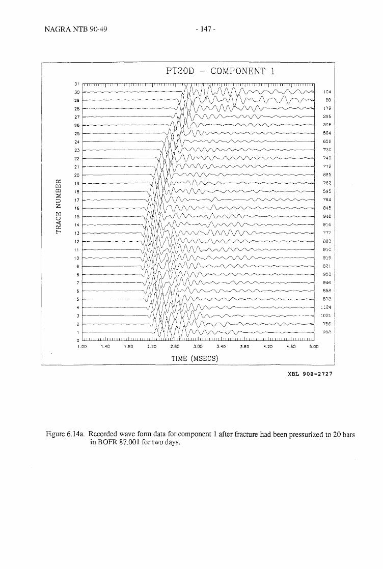
NAGRA NTB 90-49
31
.30
29
28
27
26
25
24
23
22
21
20
CC 1 9 ~ CO 18 ::E ~ 17 Z 16 (:il
15 U <t 14 c::: E- 13
12
11
10
9
B
7
6
5
.3
- 147 -
PT20D - COMPONENT 1
104
88
[')'9
295
398
564
659
73C
749
779
885
762
595
764
845
948
914
777
8C3
91C
919
821
95C
946
858
873
::24
:021
756
gge
DUli~~L~~~lill~~llllilD~~llD~~llll~~llll~lill~~~llliLUD
1.00 1.40 1.80 2.20 2.60 3.00 3.4\0 3.80 -4.20 4.60 5.00
TIME (MSECS)
XBL 908-2727
Figure 6.14a. Recorded wave form data for component 1 after fracture had been pressurized to 20 bars in BOFR 87.001 for two days.

NAGRA NTB 90-49
.31
30
29
28
27
26
25
24
23
22
21
20 cc: 19 ~ a::l ~
18
::> 17
Z 16 ~ 15 U <t 14 O! E-o 13
12
l'
10
9
B
7
6
5
4
3
2
0 1.00 1.~
- 148 -
PT20D - COMPONENT 2
TIME (MSECS)
208
156
245
377
522
622
7g0
946
1047
1155
1083
855
635
677
1019
846
877
1089
848
780
875
486
691
715
742
929
750
960
847
810
XBL 908-2728
Figure 6.14b. Recorded wave fonn data for component 2 after fracture had been pressurized to 20 bars in BOFR 87.001 for two days.

NAGRA NTB 90-49
31
30
29
28
27
26
25
24
23
22
21
20 0:: 19 ~ CD ~
18
:;:, 17 Z 16 ~ 15 U <I: 14 0:: E-o 13
12
11
10
9
8
7
6
5
4
:5
2
- 149-
PT20D - COMPONENT 3
TIME (MSECS)
14-9
114
171
282
411
572
731
783
821
621
772
663
664
616
910
821
890
861
827
612
723
600
658
735
726
74-9
713
789
832
816
XBL 908-2729
Figure 6.14c. Recorded wave fonn data for component 3 after fracture had been pressurized to 20 bars in BOFR 87.001 for two days.

NAGRA NTB 90-49 - 150-
PTOS AND PT20D AMPLITUDES - CaMP 1 PTOS AND PT20D AMPLITUDES - COMP 2 t200.0,-----------------------------------------------~
.. • • c c •
• c c
lOa. a
c • c • c
• C C
• c •
• c
• c 300. a
O.o4-~,_~,_~,_rT,_rT,_rT,_~._~_r~_r~_r~_r,,~ O.O;-rT,_rT_r~_r~_r~_r~,_rT._~_rrT_r~_r,,_r,,~ o. a 10. a
STATION
300.0
o. a
XBL 908-2730
PTOS AND PT20D AMPLITUDES - COMP 3
c c c
. .
c c . • •
STATION
c c
c c ...
10. a to. a
STATION
XBL 908-2732
Figure 6.15. Amplitude versus station number for the unpressurized data, (dark squares), and after 2 days of pressurization, (open squares) for (a) component 1, (b) component 2, and (c) component 3.
XBL 908-2731

NAGRA NTB 90-49 - 151 -
Table 6.2. Measurement schedule for pressurization of BOFR 87.001 for test PT20S.
No. Date Time P(Bars) Maximum amplitude No. of Stacks
1 24AUG 11.31 0 86.55469 16 2 24AUG 11:46 20 42.73584 10 3 24AUG 12:02 20 50.21338 10 4 24AUG 13:00 20 43.08276 10 5 24AUG 14:00 20 41.04785 10 6 24AUG 15:00 20 68.06396 10 7 24AUG 16:00 20 47.05322 10 8 25AUG 7:14 7 60.12549 16 9 25AUG 8:12 35 51.11719 10
10 25AUG 8:27 35 49.17871 10 11 25AUG 8:42 35 49.06128 10 12 25AUG 9:42 35 49.00537 10 13 25AUG 10:45 35 56.00000 10 14 25AUG 10:46 0 56.01074 10 15 25AUG 11:46 35 56.07202 10 16 25AUG 12:46 35 53.03198 10 17 25AUG 13:45 35 56.99194 10 18 25AUG 14:45 35 57.91748 10 19 25AUG 15:45 35 57.83203 10 20 25AUG 16:13 20 60.86938 10 21 26AUG 07:35 20 74.51733 10
Amplitudes are for component 1.

... 0 :::>
~ ~ C
NAGRA NTB 90-49 - 152-
PT20SS AMPLITUDES - COMP 1 PT20SS AMPLITUDES - COMP 2 100.0,-------------------------------------------------, 100.0,-------------------------------------------------,
'0.0 o
o
o 0 10.0 o
o 0
10.0 70.0
10.0
o 0 0 DOD
o 0
ao.o DOD 60.0
0
.. 0.0
lO.04--r~~--~~~~~_r~~--~T_~_r~~~r_r_T_~ 0.0 200
lO.O~-r~~--r-~._,__r~_,--~r_.-._-r_r~_,--.-~,_, 0.0 1.0 10.0 12.0 '''.0 ".0 t •• O 20.0 22. 1.0 10.0 12.0 14.0 11.0 11.0 20.0 22.
W£ASUR£W£NT W£ASUR£W£NT
XBL 908-2733 XBL 908-2734
PT20SS AMPLITUDES - COMP 3 100.0
10.0
10.0
10.0 ... 0 :::>
~ ~
o D
C o 10.0
C
o C C 0 C D
C
60.0 D
C
.0.0
lO.O 0.0 2.0 '.0 '.0 10.0 12.0 10.0 11.0 11.0 20.0 22.
Wu.sUREWENT
XBL 908-2735
Figure 6.16. Amplitude values for data given in Table 6.2 for (a) component 1, (b) component 2, and (c) component 3.

NAGRA NTB 90-49 - 153 -
this source-receiver pair has decreased from approximately 123 in PTO (Figure 6.11, COMP 1,
TRACE 28) to 86 Table 6.2, measurement 1. This illustrates the necessity of keeping the source
and receiver clamped in the exact position through out the experiment. The second measurement
was taken approximately 15 minutes after this and directly after the interval was pressurized.
This measurement shows a dramatic decrease in amplitude from 86 to 42 (Table 6.2). One would
like to think that the fracture immediately lost stiffness upon pressurization causing the amplitude
reduction. There are two reasons why this may not be true: (1.) the straight source-receiver path
intersects the fracture about 5 meters from the pressurized interval, and (2) measurement 6 (Fig
ure 6.16) taken about 3 hours later shows a large increase in amplitude, for no apparent reason.
There are just not enough ray paths taken to justify the amplitude reduction, especially since
there seems to be no other correlation throughout the rest of the experiment.
Measurement 8, taken the following day after 2 hours of depressurization again shows an
immediate increase in amplitude in accordance with the stiffness theory. The pressure is
increased to 35 bars an hour later and the amplitude again immediately decreases. The pressure
remains at 35 bars throughout the day (except for measurement 14 which measured the effect of
only about a minute depressurization; this does not show up on the pressure data which was
taken every 5 minutes). Also, throughout the day the amplitudes seem to steadily increase, with
a jump at measurement 13, which is opposite of what the stiffness theory predicts. We would
expect a steady decrease in amplitude as the pressure down the length of the fracture increased,
thus decreasing the stiffness by opening the fracture. By the end of the day (measurement 20) the
pressure is back up to where it was in the morning (measurement 8) after it was depressurized.
Therefore, we cannot say that the amplitude increased when the pressure decreased. However, by
the next day (measurement 21) the amplitude has increased. These ambiguous results are sup
ported by the sweeps PTO and PT20D as previously discussed.
Plotting the relative attenuation may show the results more clearly (Figure 6.17). This plot
shows the attenuation with respect to the first measurement which is said to have almost zero
attenuation. The figure shows the large jump between measurement 1 and 2. It also shows a con-

NAGRA NTB 90-49 - 154-
PT20 RELATIVE ATTENUATION 2. DO -,------------------------,
000
1. &0
o 0 1. DO o 0 0
o
O. &0
0.00 C 0.00 2.00 •. 00 '.00 •. 00 10.00 12.00 14.00 ".00 1'.0020.0022.0
WU.SUREWENT
XBL 908-2736
Figure 6.17. The relative attenuation between measurements for the values in Table 6.2, measurement 1 is taken as baseline. All three components have been averaged to obtain the amplitude values.
NAGRA NTB 90-49 - 155 -
sistent attenuation for the next four measurements, then more fluctuations with a general down
ward trend, opposite of what is expected, unless leak off in the region of ray coverage is occur
ring.
After the seismic measurements were made during the inflation of borehole BOFR 87.001
we wanted to perform similar measurements while borehole BOFR 87.003 was presurized.
Therefore, on 26 August the receiver was moved to 2.0 meters up the water filled borehole
BOAU 83.034 to a point adjacent to the fracture and Bofex 3 in BOFR 87.003 and clamped in
place. The close proximity of the receiver to the Bofex and the inflation point enabled us to
measure the seismic wave directly across the maximum inflation point, unlike the case when the
fracture was inflated from BOFR 87.001. Initially, a baseline sweep was taken (PTOE) down
borehole BOFR 87.002 with the source at the same points as in tests PrO, and Pr20D. The
source was then left stationary at 15.0 meters down BOFR 87.002 and hourly measurements
taken to produce data set Pf2020. The measurement schedule and amplitudes while the source
and receiver were fixed is shown in Table 6.3. The results of this sequence are similar to BOFR
87.001, however the variation in amplitudes between measurements is smaller. The amplitudes
initially seemed to decrease as required, though not significantly (Figure 6.18).
In accordance with these tests, an attempt should be made to explain why the amplitudes
varied so much between measurements. This problem is real in that each of the amplitudes in the
traces which made up the stack were consistent with each other, but different from the measure
ments taken just a few minutes later. The explanation must be that some physical change in
either the source or receiver position or the rock itself occurs in the short time span; maybe due
to the shot itself. Another explanation would be some time dependent variability in the electron
ics of the source amplitude. To determine if the amplitude variation was due to equipment or rock
condition a calibration was carried out at LBL over a two day time period. The source was
placed in a water filled borehole and the receiver was clamped into a water filled borehole
exactly in the same fashion as the field condition. The only difference being that the boreholes at
LBL were not in a fracture zone but in a 2 m x 2 m x 2 m concrete block. Measurements were

NAGRA NTB 90-49 - 156 -
Table 6.3. Measurement schedule for inflation ofBOFR 87.003
No. Date Time P (bars) Maximum Amplitude No. of Stacks
1 26AUG 12:15 0 604.0903 10 2 26AUG 12:30 20 596.0745 10 3 26AUG 12:45 20 595.1597 10 4 26AUG 13:00 20 581.0745 10 5 26AUG 13:45 20 557.0640 10 6 26AUG 14:30 20 566.1304 10 7 26AUG 15:05 20 573.7874 10 8 26AUG 16:00 20 576.5081 10 9 27AUG 10:21 20 670.8962 10
10 27AUG 10:39 20 683.5027 10 11 27AUG 10:46 20 690.5825 10 12 27AUG 11:00 0 686.8218 10 13 27AUG 11:20 0 700.6729 10 14 27AUG 11:40 0 698.1968 10 15 27AUG 12:02 0 698.4734 10 16 27AUG 13:00 0 705.7234 10 17 27AUG 14:00 0 682.1172 10 18 27AUG 15:00 0 657.0347 10 19 27AUG 15:30 0 655.7820 10 20 29AUG 7:15 0 670.8962 10 21 29AUG 7:20 0 719.9255 16
The amplitude values are from component 1.

NAGRA NTB 90-49 - 157 -
PT2020SS AMPLITUDES - COMP 1 PT2020SS AMPLITUDES - COMP 2 .• oo.o,-------------------------------------------------~
c c c c c
c c c c c c c
c c
c c o 0 c
'''.0 ".0 ' •. 0 20.0 22. 10.0 12.0 1 •. 0 ".0 1 •. 0 20.0 22.
WEASUR£W£NT WEASUR£WENT
XBL 908-2737
PT2020SS AMPLITUDES - COMP 3 •• oo.o,-------------------------------------------------~
100.0
c 0
c c C
.00.04--r_.-,--r-~,__r_r_._,--r_r_~,_-r_._,--r_~~_r~ 0.0 '0.0 12.0 ".0 ".0 ".0 20.0 22.
WEASUREWENT
XBL 908-2739
Figure 6.18. Amplitude values for a data given in Table 6.3 (a) component 1, (b) component 2, and (c) component 3.
XBL 908-2738

NAGRA NTB 90-49 - 158 -
taken at 1 hour inteIVals over two days. The signals were also recorded on a transducer per-
manently mounted on the block. This transducer would detennine if any variations were due to
source variation or the clamping of the receiver. The results were that there was no perceptible
change in the signal over a two day period. This would indicate that the changes in amplitude at
Grimsel were due to rock property changes and not clamping or electronics changes. Obviously
we did not have a simple rock type in the FRI experiment. The obseIVed changes were due to
either pressurization effects, chemical changes of the rock from injected fluid or some other fac-
tors. In any case, unfortunately, the results of the inflation experiment are such that the stiffhess
theory could not be tested in a rigorous fashion. Improvements of the experimental procedure
that may help future attempts are:
1. More measurements, both seismic and pressurelBofex should be taken.
2. The entire experiment should remain at steady state for at least a day if possible, and
3. A reference receiver should be put in place outside of the pressure zone.
6.6. Hydrologic Analysis
The storativity of a fracture can be defined as:
1 S = Ssb = pgb(¢cw + Cf) = pg(bcw + -) ,
1( (6.14)
where p is the density of water, g is the acceleration of gravity, ¢ is the porosity, which is unity,
Cw is the water compressibility, and Cf is the fracture compressibility. The fracture compressibil-
ity, Cf and the stiffhess, 1(, is related by:
1 er=bK
(6.15)
In order to calculate the stiflhess value and the specific storage using Equation (6.15) the fracture
aperture must be known. However, the aperture value is very difficult to estimate. One way to
estimate the aperture is from the transmissivity using the cubic law:
~ T= , 12Jl
(5.16)

NAGRA NTB 90-49 - 159 -
where b is the fracture aperture. As a first approximation the transient flow rate curve at 11.2 was
best-fitted to the straightforward analytical solution and the transmissivity was estimated to be
2.3 x 10⁻¹⁰m2/s. If Equation (6.16) is used to solve for b, the aperture becomes 6.6 x 10⁻⁶m.
From Equation (6.14) and the aperture value, the fracture storativity is calculated to be 5.9 x 10⁻⁸
assuming a value of K of 2 x 10¹¹ Palm (from Section 6.4). It turns out that b is so small that the
first term in Equation (6.14) is negligible.
Bofex measurements showed displacement of the fracture during the inflation tests (Figures
6.4b and 6.5b). This indicates that the fluid pressure is affecting the stress field significantly
enough to displace the fracture. The stress field change in tum can cause change in the permea
bility field. In this section we will examine the flow rate measurements to see if the fracture per
meability had changed during the inflation test.
As was briefly discussed, the injection pressure was changed three times during the
inflation test in BOFR 87.001. The initial inflation pressure in interval 11.2 was at 19 bars (Stage
1) and was raised to 35 bars at about 20 hours into the test (Stage 2). Then after five hours at 35
bars it was brought back down to about 17 bars (Stage 3). At about 50 hours the pressure was set
to about 19 bars again (Stage 4). This pressure time history is shown in Figure 6.4a. The flow
rate into interval 11.2 during the injection is shown in Figure 6.19. During Stage 4, interval 13.1
was opened to the same pressure as interval 11.2 and therefore, the flow rate in Stage 4 is the sum
of the flows into the both intervals.
If fluid pressure does not affect permeability, the flow rate (at a given time or at steady
state) should be linearly proportional to the injection pressure. Change in proportionality indi
cates change in permeability. Therefore, one can examine injectivity, which is defined as the
ratio of flow rate to injection pressure to evaluate any possible change in permeability due to
pressure change. Injectivity of BOFR 87.001 during the inflation test is shown in Figure 6.20.
As can be seen in the figure, the injectivity has increased by as much as 50% during Stage 2. The
higher pressure seems to have increased the permeability of the fracture by displacing it. During
Stage 3, the injectivity fell back to where it had been at Stage 1. This implies that the permeabil-
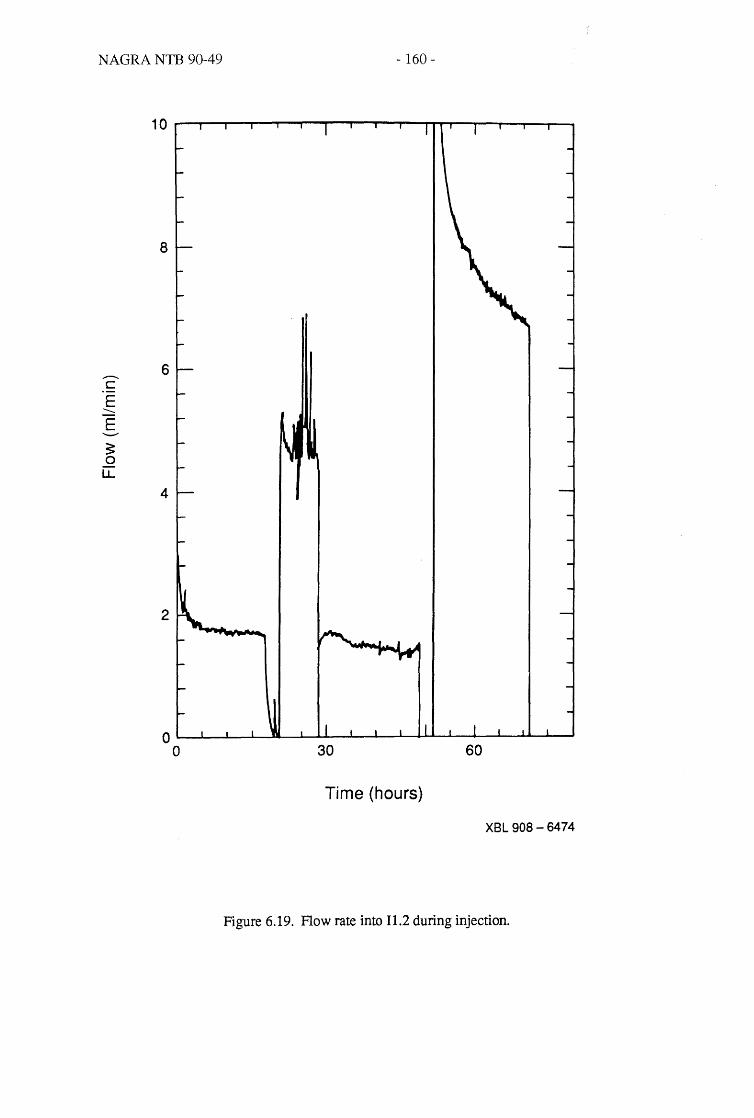
NAGRA NTB 90-49 - 160-
8
6 ...--c E
::::::: E 3: 0 u..
4
2
o~~~~~--~~--~~~~~~~~--~~~
o 30 60
Time (hours)
XBL 908 - 6474
Figure 6.19. Flow rate into 11.2 during injection.

NAGRA NTB 90-49 - 161 -
a.. .......... a
Time (hours)
XBL 908 - 6475
Figure 6.20. Injectivity (QIP) of BOFR 87.001 during the inflation test.

NAGRA NTB 90-49 - 162 -
ity had decreased back to the original value. However, the corresponding displacements meas
ured by Bofex 1 in Figure 6.4b indicate that the fracture displacement is not back to what it was
during Stage 1. This discrepancy may be due to the fact that Bofex only 'sees' displacements
occurring at the wellbore whereas injectivity is the measure of the fracture transmissivity aver
aged over the effective flow field. In other words, the fracture could have been hydraulically
back in the state it had been during Stage 1, it was mechanically still open at the well bore.
If the injectivity of the two boreholes, BOFR 87.001 and BOFR 87.003, are the same, the
injectivity during Stage 4 should be twice as large. However, as can be seen in Figure 6.20, the
injectivity almost quadrupled. This indicates that the permeability of BOFR 87.003 may be as
much as three times larger than that of BOFR 87.001. Larger injectivity of BOFR 87.001 may be
explained by the fact that BOFR 87.003 is much closer to one of the tunnels than BOFR 87.001.
It should be noted, however, that injectivity is best compared under steady-state conditions. If
transient data are used, the initial conditions should be consistent, i.e., if tests are conducted one
after another, enough time should be allowed for recovery between tests. In the present case, it
was neither at steady-state nor the same initial conditions existed for the four stages. Therefore,
the results are somewhat qualitative.

NAGRA NTB 90-49 - 163 -
7.0. SUMMARY, CONCLUSIONS, AND RECOMMENDATIONS
The motivation for the FRI project was to improve our abilities to use seismic imaging as a
tool for characterizing fractured rock, particularly for the purpose of hydrologic analysis. We
chose a fracture zone which was clearly present, hydrologically conductive, and accessible so
that we could test, calibrate, and improve our abilities to image and characterize such a feature
with seismic tomography. Four other studies were conducted in association with the seismic
experiments. A detailed geologic investigation provided the appropriate background and insight
for interpretation of the tomograms. Geomechanical studies allowed controlled measurement of
the rock and fracture properties and allowed us to develop hypotheses to help interpret the results
from the tomographic studies. A limited number of hydrologic tests were used to check the visual
observation that the fracture zone was hydrologically active and to see if other features marked
by seismic anomalies might also conduct fluid. Finally, we attempted to significantly modify the
fracture zone properties by inflating the kakirite fracture, measuring its stiflhess and permeability
change in situ, in order to determine if we could simultaneously detect changes in the seismic
response.
The site of the FRI experiments was picked because upon initial visual inspection, it
appeared structurally simple and it was accessible from four sides. However, as more detailed
investigations were performed, it became clear that the site is not at all simple. The rock is
heterogeneous and anisotropic. In addition to the main shear zone, there are different granitic
rock types, lamprophyres interspersed in the rock, fractures or joints, and mineralized veins. The
excavation of the tunnels bounding the FRI site apparently caused significant additional fractur
ing at the tunnel walls.
Laboratory results indicated that the level of saturation has a dominant effect on P- and S
wave velocities and amplitudes. The velocity was significantly lower and the attenuation was

NAGRA NTB 90-49 - 164-
greater in dry samples than in saturated samples. We could not test the effect of the kakirite frac
ture in the laboratory because the core containing it was reduced to rubble. The effect of smaller,
but still macroscopic fractures that we could test was not found to be significant. The effect of
heterogeneity in the rock was exemplified by one of the fractured specimens which had a higher
velocity than the adjacent intact rock specimens. This highlights an important aspect of using
seismic information to locate and characterize fractures: the seismic tomography is imaging
mechanical properties and not all of these mechanical properties may be correlated to hydrologic
properties.
The tomographic images produced in 1987 and 1988 are different. The major fractures con
taining kakirite were imaged clearly as Feature A in the 1987 velocity tomogram. In the 1988
tomogram, the feature is still imaged, but it is not as pronounced. The damaged zones near the
tunnel walls are clearly seen in 1987 and are not obvious in 1988.
Several hypotheses to explain the differences in the two surveys were explored first, if the
rock in the vicinity of Feature A and in the tunnel damage zone had been more saturated in 1988
than in 1987 due to fluid injection just prior to the 1988 seismic testing, laboratory results indi
cate that the fracture zone would have been characterized by a higher velocity and lower attenua
tion in 1988 and would have therefore produced a smaller seismic anomaly. However, there is no
strong evidence to show that the rock was not saturated in 1987.
Different sources and coupling mechanisms were used in the two years, so the reason for
the differences in the tomograms might be that the seismic source used in 1987 was not as power
ful. Thus the first arrivals of waves which were severely attenuated as they passed through the
shear zone and the damaged zones near the drifts were not detected in 1987. Having missed the
first arrivals the velocity appeared to be slower. The first arrivals were seen in 1988 and the zone
was a weaker velocity anomaly.
Probably the most interesting hypothesis for increased attenuation in 1987 is that frequency
differences between 1987 and 1988 were the cause of the different images. The dominant fre
quency of the received signal used in 1987 was lower than in 1988. By calculating values of
NAGRA NTB 90-49 - 165 -
stiflhess at the 1987 and 1988 dominant frequencies, we have shown that this difference in fre
quency would result in significantly more delay through the fracture in 1987 than in 1988. Thus,
stiflhess theory alone could account for the smaller anomalies in 1988. This unintentional change
in frequency may have resulted in the best evidence so far for the applicability of stiflhess theory
to acoustic wave propagation in fractured media. The 1987 results essentially combined attenua
tion and velocity tomography through serendipity, but it may be beneficial to look for frequencies
which combine attenuation and velocity tomography by design.
The hydraulic tests that were conducted confinned the hydrologic significance of the
kakirite-bearing fractures in the FRI zone identified by the seismic tomography. Conduction
along the zone was observed, but the hydraulic response curves did not indicate flow in an
infinite plane. Several scenarios which could effectively cause leakage were examined to see if
they could explain the deviations. The boundary effect caused by drainage into the tunnels seems
to be very small. It is possible that the leakage from the FRI fracture may occur locally though
another feature that intersects it. There is evidence from the hydrologic tests for some permeabil
ity perpendicular to the fracture which may correspond to features identified through tomography
in the FRI site. If the PRI work continues, we recommend that holes be drilled into these other
features to validate the tomographic results. Further hydrologic testing should also be conducted
to determine the behavior of these features. Tracer tests may also help us further characterize the
hydrology of PRI fractures. In any case, the interaction between the seismic and well test results
showed how the seismic results could be used to guide the well test design and the well test
interpretation could be used to develop hypotheses for further seismic and hydrologic testing.
A method for in-situ determination of mechanical stiflhess of a fracture was successfully
demonstrated. In this regard it was shown that corrections for the limited areal extent of the
inflation pressure in a fracture can significantly affect how such measurements should be inter
preted. The lack of any consistent observable change in the associated seismic measurements
was also most likely due to the limited extent of fracture inflation. Furthennore, it is clear that a
future test should be carried out under more controlled conditions being sure that more measure-

NAGRA NTB 90-49 - 166 -
ments are taken and a reference path is used. As a result of these short comings, the joint
geomechanical and seismic measurements were inconclusive in confirming the fracture stiffuess
theory.
Hydraulic storativity, which is notoriously hard to estimate, was independently estimated
for the FR.I fracture using the geomechanics measurements. This work represents new possibili
ties for joint mechanical and hydrologic well test interpretation. Further independent mechanical
measurement might provide a new way to explain the apparently non-linear flow behavior often
observed in well tests in fractured rock.
An interesting sidelight of the seismic work was that the damage zones caused by mining
are significant seismic anomalies that can be defined by tomography. This information might be
very useful in a mine-by experiment designed to evaluate the effect of excavation. Some of the
seismic perturbation might be due to desaturation, and it would be very elucidating to repeat such
measurements over time following excavation.
The seismic work points to several other promising areas for new work. The greatest poten
tial use for the seismic methods lie in the combined use of P- and S-wave analyses, although to
date there are no adequate high frequency S-wave sources available. None of the sources tried at
the FRI site produced good S-waves. Also, large amounts of data are necessary for tomographic
imaging. Hundreds of thousands of traces may be collected. These must be taken back to the
office and the first arrivals picked by hand in order to prepare the data for tomographic inversion.
Many problems with the field data may not show up for months after the data are collected. If
in-field, real-time data processing were developed, experimenters could see the results of the data
processing as the data were collected. This would speed up the analysis and allow problems with
the data to be identified and corrected in the field.
The FR.I site is not as simple as we had originally envisioned, and consequently the results
of the individual testing programs are not unequivocal. However, the combined results clearly
show how seismic methods can be more effectively applied to image fractured rock. In addition,
we have gained a better understanding of the relative significance of the physical properties

NAGRA NTB 90-49 - 167 -
affecting the propagation of seismic energy and the importance of the seismic results relative to
the hydrologic properties of fractured rock. Although the work was primarily carried out in
saturated, fractured granite, the results are focused on the physics of the processes and thus appli
cable to almost any rock that is dominated by fracture permeability.

NAGRA NTB 90-49 - 169-
8.0. REFERENCES
Carslaw, H. S. and J. C. Jaeger, 1946. In Conduction of Heat in Solids, Clarendon Press, Oxford.
Crampin, S., 1978. Seismic-wave propagation through a cracked solid: Polarization as a possible dilatancy diagnostic, Geophys. 1. Roy. Astron. Soc., 53, 467-496.
Crampin, S., 1981. A review of wave motion in anisotropic and cracked elastic-media, Wave Motion, 3, 343-391.
Cram pin, S., 1984a. Effective anisotropic propagation through a cracked solid, In Crampin, S., Hipkin, R. G., and Chesnokov, E. M., eds., Proc. of the First International Workshop on Seismic Anisotropy, Geophys. J. Roy. Astron. Soc., 76,135-145.
Crampin, S., 1984b. Anisotropy in exploration seismics, First Break, 2, 19-21.
Crampin, S., 1985. Evaluation of anisotropy by shear wave splitting, Geophysics, 50, (1) 142-152.
Crouch, S. L. and A. M. Starfield, 1983. Boundary Element Methods in Solid Mechanics: With Applications in Rock Mechanics and Geological Engineering, Allen and Unwin, London, Boston.
Da Prat, G., H. Cinco-Ley, and H. J. Ramey, Jr., 1981. Decline curve analysis using type curves for two-porosity systems, Society of Petroleum Engineers Journal, Society of Petroleum Engineers of AIME, 354-362.
Ehlig-Economides, C. A., 1979. Well test analysis for wells produced at a constant pressure, Ph.D. Thesis, Stanford University, Stanford, California.
Geotest, 1988. Felslabor Grimsel Fracture Zone Investigation, 3052 Zollikofen!Bern, Switzerland.
Hopkins, D. L., N. G. W. Cook, and L. R. Myer, 1987. Fracture stiffuess and aperture as a function of applied stress and contact geometry, Proc. 28th U.S. Symp. Rock Mech., Dniv. of Arizona, Tucson, Arizona, June 29-July 1, 1987.
Johnson, L. R. and J. E. Peterson, 1986. Analysis of ultrasonic velocities in Kouros, LBL Report LBID-1175.
Kucuk, F. and Brigham, W. E., 1979. Transient flow in elliptical systems, Soc. Pet. Eng. J., 401-410.
Nagra Technical Report 85-46, 1985. Grimsel Test Site - Overview and test programs, Baden, Switzerland, 118 pp.
Pyrak-Nolte, L. J., L. R. Myer and N. G. W. Cook, 1990. Anisotropy in seismic velocities and amplitudes from multiple parallel fractures, J. Geophys. Res., (in press).
Pyrak-Nolte, L. J., L. R. Myer and N. G. W. Cook, 1989. Transmission of seismic waves across single fractures J. Geophys. Res., (in press).
Schoenberg, M., 1980. Elastic wave behavior across linear slip interfaces, J. Acoust. Soc. Am., 68, (5) 1516-1521.

NAGRA NTB 90-49 - 170-
Schoenberg, M., 1983. Reflection of elastic waves from periodically stratified media with interfacial slip, Geophys. Prosp., 31,265-292.
Van Everdingen, A. E, W. Hurst, 1949. The application of the Laplace Transfonnation to flow problems in reservers, Trans., A/ME, 186, 305-324.
Wyss, E., 1988. Kurzbericht Zu Den Ersten Hydrogelogischen Untersuchungen 1m Rahmen Des Versuches FRI, 616, NAGRA, Internal Data Report.
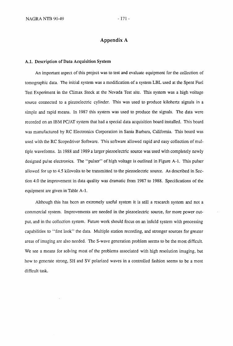
NAGRA NTB 90-49 - 171 -
Appendix A
A.1. Description of Data Acquisition System
An important aspect of this project was to test and evaluate equipment for the collection of
tomographic data. The initial system was a modification of a system LBL used at the Spent Fuel
Test Experiment in the Climax Stock at the Nevada Test site. This system was a high voltage
source connected to a piezoelectric cylinder. This was used to produce kilohertz signals in a
simple and rapid means. In 1987 this system was used to produce the signals. The data were
recorded on an IBM PCI AT system that had a special data acquisition board installed. This board
was manufactured by RC Electronics Corporation in Santa Barbara, California. This board was
used with the RC Scopedriver Software. This software allowed rapid and easy collection of mul
tiple waveforms. In 1988 and 1989 a larger piezoelectric source was used with completely newly
designed pulse electronics. The' 'pulser" of high voltage is outlined in Figure A-t. This pulser
allowed for up to 4.5 kilovolts to be transmitted to the piezoelectric source. As described in Sec
tion 4.0 the improvement in data quality was dramatic from 1987 to 1988. Specifications of the
equipment are given in Table A-I.
Although this has been an extremely useful system it is still a research system and not a
commercial system. Improvements are needed in the piezoelectric source, for more power out
put, and in the collection system. Future work should focus on an infield system with processing
capabilities to "first look" the data. Multiple station recording, and stronger sources for greater
areas of imaging are also needed. The S-wave generation problem seems to be the most difficult.
We see a means for solving most of the problems associated with high resolution imaging, but
how to generate strong, SH and SV polarized waves in a controlled fashion seems to be a most
difficult task.

NAGRA NTB 90-49
PSl (+)
HIGH VOLTAGE POWER SUPPLY
0-4 KVDC (-)
"FAST SWITCH" (HYDROGEN THYROTRON)
FAST OUT SLOW OUT
INTERNAL PULSE GENERATOR
& DRIVER UNIT
EXT. TRIG IN EOT TRIG OUT
START COMP TRIG OUT
GATE DR MON SCOPE TRIG OUT OUT
- 172 -
HV PULSER SYSTEM
I_ DISTANCE APPROX 200 FT. - 500 FT. • I r-----------------------L _ _ _ _ _ _ _ _ _ _ _ _ _ PIEZOELECTRIC TRANSDUCER
C3
C4
VDl t--+--+-_ HV PULSE
OUTPUT MONITOR
1 1 IR : L 1- __
C L 1
1 - ______ 1
R:::::1 MEG L
C :::::0.02 UF L .- -- - - - --- --."
I I .-------TYPICAL TIMING -------.
200 NS 1 - 10 MS MAX (TYP) 200 NS
~ I~~:oo MS (ryP) I ~' -I F SCOPE II ' I I
TRIG _ _ ' , , II II
COMPUTER n ' I I TRIG ~~,
GATE DRIVE ~0 : MONITOR _ _ :
EOT I I ,~,~----------TRIG I n
_______ I , ~ '---------
FASTSW 1\' ~', " -E1 V , I,;:~
SLOEW2
SW 1"'1--.: iF ~ : [1,'..---
HV PULSE 1....1 -' -----.iP,p..' ------f~ OUTPUT MON. I I I I , XBL 908-2815
Figure A-I. HV pu1ser system.

NAGRA NTB 90-49 - 173 -
Table A.I. Specifications of data acquisition system
Piezoelectric Source
Stack of 4 cylindrical Navy 5500 piezoelectric material. Each element in stack is 3 inches in diameter, 2 inches high and 1/4 inch wall thickness.
High Voltage Pulser
The "high voltage pulser" provides the necessary voltage to excite a piezoelectric transducer. The pulser unit consists of the following: (see Figure A.I)
(1) A variable high voltage power supply, 0 to 4.? kVdc, HVPS.
(2) An energy storage and electronic switching system.
(3) An internal pulse generator and driver unit.
(4) A precision high voltage pulse output monitor, VD1.
The high voltage power supply (HVPS):
The HVPS provides a variable dc source of high voltage (0 to 4.5 kVdc) necessary to charge the energy storage system capacitors, C1 and C2. The maximum current available from the HVPS is 50 mAdc.
The energy storage and electronic switching system:
The purpose of this section of the HV pulser is to provide the piezoelectric transducer with a very short rise time, long duration, negative high voltage pulse with adjustable amplitude.
This pulse is generated by using two independent capacitors: switching circuits, namely the fast switch and the slow switch.
The fast capacitor switch circuit consists of R 1, C 1 and V 1. The slow circuit consists of R2, C2 and V2.
Please refer to Figure A-I for circuit and timing details.
The internal pulse generator and driver unit
The pulse generator and drive units provides the necessary gates and triggers required for proper operation of the high voltage pulser.
Output triggers are provided to the computer indicating the start of the output pulse and end of the pulse.
Please refer to Figure A-I for "typical timing."
The precision high voltage pulse output monitor.
The output HV pulse monitor provides an output of IOOOv/v, into 50 ohms. The pulse rise and fall time of this circuit is good enough to observe the main hv pulse with reasonable fidelity.
Data Storage
IBM PC/AT with 2 Mb of RAM. RC Electronics, Inc. "scope driver" system. Data throughput of 1 million samples/sec over 16 channels maximum. 64,000 data points collected, per "shot." Capability to stack in real time up to 10,000 shots. Various offline analysis software.