Technical Report: Joint Power and Antenna

Selection Optimization in Large Distributed

MIMO NetworksAn Liu, Vincent Lau, Fellow IEEE,

Department of Electronic and Computer Engineering, Hong Kong University of Science and Technology

Abstract

Large MIMO network promises high energy efficiency by employing a large number of antennas.

However, the overhead to obtain the full channel state information is very large. To reduce the overhead,

we propose a downlink antenna selection scheme, which selects a subset of antennas based on the

knowledge of large scale fading factors to serve a given set of users in large distributed MIMO networks

employing regularized zero-forcing precoding. We study the joint optimization of antenna selection,

regularization factor, and power allocation to maximize the average weighted sum-rate. The problem is

a mixed combinatorial and non-convex problem whose objective and constraints have no closed-form

expressions. Random matrix theory is used to derive asymptotically accurate expressions for the objective

and constraints. The joint optimization problem is decomposed into three subproblems, each of which

is solved by an efficient algorithm. We derive structural solutions for some special cases and obtained

the capacity scaling law under very large distributed MIMO networks. We also show that for sufficiently

large number of distributed antennas, there is an asymptotic decoupling effect, which can be exploit

to simplify algorithms and physical layer processing. Simulations illustrate that the proposed scheme

achieves significant performance gain compared with various baselines.

Index Terms

Large MIMO network, Cloud Radio Access Networks (C-RAN), Antenna selection, Asymptotic

Analysis

I. INTRODUCTION

Large MIMO network has been a hot research topic lately due to the potentially high energy efficiency

[1]. Such a network is equipped with an order of magnitude more antennas than conventional systems.

For a base station (BS) with M 1 antennas, the total transmit power can be made as O (1/M), and the

transmit power per antenna would be O(1/M2

)[2]. Furthermore, the gain in multiuser system is very

impressive due to the increased degrees of freedom for large MIMO systems. There have been plenty of

works on large MIMO networks, including various topics from information theoretical capacity [3], [4]

to more practical issues such as transceiver design [5]–[7], channel state information (CSI) acquisition,

and pilot contamination problem [8], [9]. Various downlink precoding schemes have been proposed and

analyzed. Remarkably, the simple zero-forcing precoding is shown to achieve most of the capacity of

large MIMO downlink [2]. One of the main challenges of achieving the performance predicted by the

idea analysis is how to obtain the CSI at the transmitter (CSIT) for a very large number of antennas

with acceptable amount of overhead. In most of the existing works, Time-Division Duplex (TDD) is

assumed and channel reciprocity can be exploited to obtain CSIT via uplink pilot training. However,

there is still no efficient method for CSIT training and feedback in Frequency-Division Duplex (FDD)

networks. In [10], [11], random matrix theory has been used to analyze the asymptotic performance of

zero-forcing (ZF) and/or regularized ZF (RZF) [12], with focus on the case when all the antennas are

collocated at a BS. In [13], the authors provided a unified large system analysis of the performance of

linear detectors/precoders in multicell multiuser TDD systems under a general channel model.

In this paper, we focus on large distributed MIMO networks in which there are M distributed antennas

(thin base stations) linked together by high speed fiber backhaul as illustrated in Fig. 1. This distributed

network is also called the Cloud-RAN [14]. In such a scenario, it is likely that only a few nearby

antennas (thin base stations) can contribute significantly to a user’s communication due to path loss. To

avoid expensive CSI acquisition and signal processing overheads for antennas with huge path loss to the

users, a subset of S active antennas is selected to serve a given set of K users using RZF precoding,

where M S ≥ K. RZF precoding is considered because it is asymptotically optimal for S,K → ∞

[15], and it is more tractable than the more complicated non-linear precoding schemes.

There are some works studying antenna selection problems in multi-user MIMO systems [16], [17].

However, these approaches require the global knowledge of the instantaneous CSI in the network which

causes unacceptable signaling overhead for large M . This problem could be avoided using a simple

antenna selection algorithm which associates each user with the “strongest” antennas/BSs (i.e., the

antennas/BSs who have the largest path gain with the user). This simple baseline algorithm has been

adopted in conventional cellular networks such as 3G and LTE systems. However, it is inefficient when

the antennas/BSs are allowed to perform cooperative MIMO (CoMP) [18] as illustrated in the following

two examples. In both examples, we assume S = 2 distributed antennas are selected to serve K = 2

Cloud RAN

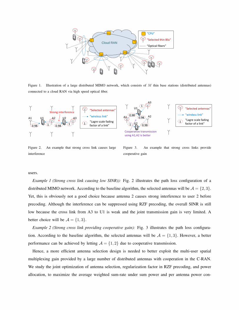
Figure 1. Illustration of a large distributed MIMO network, which consists of M thin base stations (distributed antennas)

connected to a cloud RAN via high speed optical fiber.

Figure 2. An example that strong cross link causes large

interference

!"#$

Figure 3. An example that strong cross links provide

cooperative gain

users.

Example 1 (Strong cross link causing low SINR)): Fig. 2 illustrates the path loss configuration of a

distributed MIMO network. According to the baseline algorithm, the selected antennas will be A = 2, 3.

Yet, this is obviously not a good choice because antenna 2 causes strong interference to user 2 before

precoding. Although the interference can be suppressed using RZF precoding, the overall SINR is still

low because the cross link from A3 to U1 is weak and the joint transmission gain is very limited. A

better choice will be A = 1, 3.

Example 2 (Strong cross link providing cooperative gain): Fig. 3 illustrates the path loss configura-

tion. According to the baseline algorithm, the selected antennas will be A = 1, 3. However, a better

performance can be achieved by letting A = 1, 2 due to cooperative transmission.

Hence, a more efficient antenna selection design is needed to better exploit the multi-user spatial

multiplexing gain provided by a large number of distributed antennas with cooperation in the C-RAN.

We study the joint optimization of antenna selection, regularization factor in RZF precoding, and power

allocation, to maximize the average weighted sum-rate under sum power and per antenna power con-

straints. The optimization requires the knowledge of large scale fading factors only and the overhead for

CSI acquisition is greatly reduced as discussed in Remark 1. The following are two first-order technical

challenges that need to be addressed.

• Combinatorial Optimization Problem: As motivated by the examples, traditional antenna selection

scheme in which each user is associated with the closest antennas (thin base stations) is highly sub-

optimal in the CoMP configuration. In fact, the antenna selection problem with CoMP processing

in the C-RAN is combinatorial with exponential complexity w.r.t. the total number of antennas M .

Brute force solution requires exhaustive search which is highly undesirable.

• Asymptotic Performance Analysis: It is also important to derive closed-form performance ex-

pressions for the C-RAN with dynamic antenna selection supporting CoMP in order to obtain

design insights on how the network performance scale with important system parameters. Yet, the

performance analysis is highly non-trivial due to the heterogeneous path loss between antenna-user

pair as well as the lack of closed form antenna selection solution.

In this paper, we first outline the system model and the antenna selection formulation in Section II

and III. Using the random matrix theory, we extend the results in [11] to obtain asymptotically accurate

expressions for the weighted sum-rate objective and the per-antenna transmit power constraints under a

given antenna selection and power allocation. By exploiting the implicit structure in the objective and

constraints functions, the joint optimization problem is decomposed into simpler subproblems, each of

which is solved by an efficient algorithm in Section IV. In Section V, we focus on studying the structural

properties of the solution for some interesting special cases and the asymptotic performance analysis for

very large distributed MIMO networks. For large M , we show that there is an asymptotic decoupling

effect in the distributed MIMO networks and the capacity grows logarithmically with M even when the

number of active antennas S is fixed. Simulations in Section VI illustrate that the proposed solution

achieves significant performance gain compared with various baselines.

II. SYSTEM MODEL

A. Channel Model

Consider the downlink of a large distributed MIMO network with M distributed transmit antennas

and K single-antenna users as illustrated in Fig. 1. The M K transmit antennas are distributed

geographically and connected to a Cloud RAN [14] via high speed fiber backhaul. Denote hkm as the

channel between the mth transmit antenna and the kth user. We consider composite fading channel, i.e.,

hkm = σkmWkm, ∀k,m, where σkm ≥ 0 is the large scale fading factor caused by, e.g., path loss and/or

shadow fading, and Wkm is the small scale fading factor.

Assumption 1 (Composite fading channel model): The small scale fading process Wkm (t) ∼ CN (0, 1)

is quasi-static within a time slot but i.i.d. w.r.t. time slots and the spatial indices k,m. The large scale

fading process σkm (t) is assumed to be a slow ergodic random process according to a general distribution.

It is also independent w.r.t. the spatial indices k,m.

B. Physical Layer Processing

We assume M K in the distributed MIMO network. While the M antennas are geographically

distributed in the coverage area, the baseband processing is centralized at the cloud RAN. To limit the

pilot training and signal processing overheads to serve the K users, we consider antenna selection scheme

where only a subset A, |A| = S ≥ K of the M distributed antennas are selected (activated) to serve the

K users. For convenience, let Aj denote the jth element in A. Let H (A) ∈ CK×S denote the composite

downlink channel matrix between the selected S antennas and the K users, and define Σ (A) ∈ RK×S++

as the corresponding large scale fading matrix, whose element at kth row and the jth column is σkAj . In

the rest of the paper, we will use H and Σ as the simplified notations for H (A) and Σ (A) when there

is no ambiguity. The cloud RAN is assumed to have knowledge of the K ×M large scale fading factors

σkm’s for antenna selection but only the K×S channel matrix H (A) for cooperative MIMO processing.

Remark 1 (Long-term and short-term CSI Acquisition): In TDD systems, channel reciprocity can be

exploited and H (A) can be estimated at the cloud RAN by transmitting reference signals in the uplink.

In FDD systems, the short-term channel matrix estimation H (A) can be obtained via explicit channel

feedback. In both cases, the amount of training for the short-term channel matrix H (A) is limited by the

coherence time of the channel. Since the channel coherent time is O(1), estimated CSI quality H (A) at

the C-RAN will be very poor if all the antennas in the network are active. Using antenna selection, the

number of active antennas at any time slot is limited. Hence, the amount of instantaneous CSI feedback

or the uplink overheads of channel sounding is greatly reduced by antenna selection A. On the other

hand, estimating the large scale fading matrix Σ is not limited by the channel coherent time because it is

a long-term statistics. In both FDD and TDD systems, the large scale fading matrix Σ can be estimated

at the C-RAN from the uplink reference signals [19], [20] due to the reciprocity of large scale path loss.

We consider linear precoding processing to support simultaneous downlink transmissions to the K

users using the set of active antennas A. The K × 1 composite receive signal vector for the K users can

be expressed as:

y = HFs + n,

where s = [s1, ..., sK ] ∼ CN (0, IK) is the symbol vector, F = [f1, ..., fK ] ∈ CS×K is the precoding

matrix and n ∼ CN (0, IK) is the AWGN noise vector. We employ regularized zero-forcing (RZF)

precoding [12] which is given by

F =(H†H + αIS

)−1H†P1/2 = H†

(HH† + αIK

)−1P1/2, (1)

where α is the regularization factor and P = diag (p1, ..., pK) is a power allocation matrix. Define power

allocation vector as p = [p1, ..., pK ]T . Note that the above RZF is a generalization of the conventional

RZF in [12], where P is fixed as cIK and c is chosen to satisfy sum power constraint.

For convenience, define the normalized channel matrix H = H/√S and normalized regularization

factor ρ = α/S. Let h†k denote the kth row of H and H1j denote the jth column of H, where 1j denotes

a K×1 vector of which the jth element is 1 and all other elements are zeros. Define Hk as the matrix H

with the kth row removed, and Pk , diag (p1, ..., pk−1, pk+1, ..., pK) . We assume that user k has perfect

knowledge of the effective channel h†kfk and the interference-plus-noise power, which can be estimated

through dedicated downlink training. Under this assumption and using matrix inversion lemma, it can be

shown that the SINR of user k is given by [10]

γk (Σ, ρ,p) =pkA

2k

Bk + (1 +Ak)2 , (2)

where

Ak = h†k

(H†kHk + ρIS

)−1hk,

Bk = h†k

(H†kHk + ρIS

)−1H†kPkHk

(H†kHk + ρIS

)−1hk.

The transmit power of the jth selected antenna in A is given by

pAj (Σ, ρ,p) = 1Tj H†(HH† + ρIK

)−1P(HH† + ρIK

)−1H1j/S. (3)

III. OPTIMIZATION FORMULATION FOR DYNAMIC ANTENNA SELECTION

A. Optimization Variables, Objective and Constraints

In this paper, we consider the joint optimization of active antenna set A, regularization factor ρ and

the power allocation p. The optimization is performed over the time scale of large scale fading, i.e., A,

ρ and p are only adaptive to the large scale fading factors. The objective is to maximize the weighted

sum-rate averaged over one large scale fading block. Given a realization of σkm’s and an active antenna

set A, the large scale fading matrix Σ (A) is fixed within a large scale fading block, and the conditioned

average weighted sum-rate is given by

I (A, ρ,p) = E

[K∑k=1

wklog (1 + γk (Σ (A) , ρ,p)) |Σ (A)

], (4)

where the conditioned expectation E [· |Σ (A) ] is taken over the small scale fading factors, and wk ≥ 0

is the weight for user k. We consider both per antenna and sum power constraint, which are given by

E [pm (Σ (A) , ρ,p) |Σ (A) ] ≤ pm, m ∈ A, (5)

E

[∑m∈A

pm (Σ (A) , ρ,p) |Σ (A)

]≤ PT . (6)

B. Problem Formulation

The optimization problem is formulated as follows

maxA,ρ>0,p≥0

I (A, ρ,p) , s.t. (5) and (6) are satisfied, |A| = S. (7)

There are several challenges to solve Problem (7). First, there is no analytical expression for the

optimization objective in (4) and the constraints in (5) and (6). Second, determining the optimal A in

(7) requires an exhaustive search over the entire antenna set. Third, even for fixed A, the problem is in

general non-convex w.r.t. ρ and p, as will be shown later. In this paper, the first challenge is tackled

in this section by using the random matrix theory in [11] to derive asymptotically accurate expressions

for the optimization objective and constraints. The last two challenges are tackled by decomposing the

problem into simpler subproblems, each of which is solved by an efficient algorithm in Section IV.

To derive asymptotically accurate deterministic expressions, we require the following assumptions.

Throughout the paper, the notation SK=Sβ−→ ∞ refers to K,S →∞ such that lim

S→∞K/S = β ∈ (0,∞).

Assumption 2 (Boundedness of Large Scale Fading): The elements of the large scale fading matrix

Σ (A) are uniformly bounded on S, i.e.,

lim supSK=Sβ−→ ∞

sup1≤k≤K, m∈A

|σkm| < ∞.

Moreover, 1S

∑Kk=1 σ

2km, ∀m ∈ A is uniformly lower bounded by some nonnegative quantity, i.e.,

lim infSK=Sβ−→ ∞

infm∈A

1

S

K∑k=1

σ2km > 0.

The normalized channel matrix H (A) has uniformly bounded spectral norm on S with probability 1,

i.e.,

lim supSK=Sβ−→ ∞

∥∥∥H† (A) H (A)∥∥∥ < ∞,

with probability one, where ‖·‖ denotes the spectral norm of a matrix.

The power allocation p satisfies max (p1, ..., pK) = O (1/K).

In the following, we derive asymptotic expressions for the SINR and per-antenna power constraints

under Assumption 2 in large system limit when K,S →∞ with the ratio β = K/S fixed.

Lemma 1 (Asymptotic SINR): Based on Assumption 2, the following statements are true for any given

(A, ρ > 0,p).

1) The system of K equations:

ξl =1

S

∑m∈A

[σ2lm/fm

(~ξ)], l = 1, ...,K, (8)

admits a unique solution ~ξ = [ξ1, ..., ξK ]T in RK+ , where fm(~ξ), ρ+ 1

S

∑Ki=1

σ2im

1+ξi.

2) Define matrix D ∈ RK×K whose element at the lth row and nth column is given by

Dln =1

S

∑m∈A

[1

Sσ2lmσ

2nm/

((1 + ξn)2 f2

m

(~ξ))]

.

Define vector b = [b1, ..., bK ]T whose lth element is given by

bl = − 1

S

∑m∈A

[σ2lm/f

2m

(~ξ)].

For any k ∈ 1, ...,K, define vector dk = [dk1, ..., dkK ]T whose lth element is given by

dkl =1

S

∑m∈A

[σ2kmσ

2lm/f

2m

(~ξ)].

Then IK −D is invertible and thus we can define the following vectors

~φ , (IK −D)−1 b, (9)

~θk , (IK −D)−1 dk, k = 1, ...,K, (10)

where the lth element of ~φ, denoted by φl, is the partial derivative of ξl over ρ.

3) Let γk (Σ, ρ,p) be the SINR of user k defined in (2). As K,S → ∞ with the ratio β = K/S

fixed, we have γk (Σ, ρ,p)− γk (Σ, ρ,P)a.s→ 0, where

γk (Σ, ρ,P) =pkξ

2k

1S

∑Kl 6=k

[plθkl/ (1 + ξl)

2]

+ (1 + ξk)2, (11)

where θkl is the lth element of ~θk.

Lemma 2 (Asymptotic per-antenna power): Based on Assumption 2, the following statements are true

for any given (A, ρ > 0,p).

1) The system of K equations:

vl =1

ρ+ 1S

∑m∈A

[σ2lm/ψm (v)

] , l = 1, ...,K (12)

admits a unique solution v = [v1, ..., vK ]T in RK++, where ψm (v) , 1 + 1S

∑Ki=1 σ

2imvi.

2) Define a matrix C ∈ RK×K whose element at the lth row and nth column is given by

Cln =1

S

∑m∈A

[1

Sσ2lmσ

2nmvl/ψ

2m (v)

]. (13)

Define a diagonal matrix ∆ with the lth diagonal element given by

∆l =1

S

∑m∈A

[σ2lm/ψm (v)

]. (14)

Define a vector c = [c1, ..., cK ]T with the lth element given by

cl =1

S

∑m∈A

[σ2lmvl

(pl +

1

S

K∑i=1

σ2imvi (pl − pi)

)/ψ2

m (v)

].

Then ρIK + ∆−C is invertible and thus we can define the following vector

~ϕ , (ρIK + ∆−C)−1 c. (15)

3) Let pm (Σ, ρ,p) be the per-antenna power defined in (2). As K,S →∞ with the ratio β = K/S

fixed, we have pm (Σ, ρ,p)− pm (Σ, ρ,p)a.s→ 0, ∀m ∈ A, where

pm (Σ, ρ,p) =ρ−1

S2ψ−2m (v)

K∑i=1

σ2im (pivi − ϕi) , ∀m ∈ A, (16)

where ϕi is the ith element of ~ϕ in (15).

Please refer to Appendix A for the proof of the above two lemmas.

Remark 2: The equations in (8) and (12) can be solved using the fixed point iterations in Proposition

1 of [11].

Remark 3: Another deterministic approximation of the SINR has been provided in Theorem 2 of [11].

The differences between the deterministic approximation in (11) and the one in [11] are as follows. 1)

In [11], a more general channel model which includes per-user channel transmit correlation and channel

estimation error is considered. Our channel model is a special case of the channel model in [11] with the

channel correlation matrices given by Θk = diag(σ2km, m ∈ A

), ∀k and zero channel estimation error,

i.e., τk = 0 in [11]. Since we assume geographically distributed antennas, the correlations between the

antennas are indeed negligible. Moreover, the algorithms and most results in this paper can be directly

generalized to case with transmit correlation and channel estimation error with little modification. 2) We

consider both sum power constraint and per-antenna power constraint, while [11] focused on sum power

constraint only. Consequently, in the deterministic approximation in [11], the precoding matrix F is scaled

to satisfy the sum power constraint. However, it is impossible to satisfy the per-antenna power constraint

by simply scaling F. Hence, the deterministic approximation in (11) is for a given power allocation p

without scaling of F. Moreover, we need to derive the deterministic approximation for per-antenna power

constraint in (2), which is not given in [11]. Then the per-antenna power constraint is guaranteed by the

optimization algorithm.

For convenience, define pA (Σ, ρ,p) ,∑

m∈A pm (Σ, ρ,p). Using the above two lemmas and follow-

ing similar proof as that of [21, Prop. 1], we can prove the following theorem which gives an asymptotic

equivalence of Problem (7).

Theorem 1 (Asymptotic equivalence of Problem (7)): Assume that Assumption 2 is satisfied. Let A∗,

ρ∗,p∗ denote an optimal solution of the following optimization problem

PE : max I (A, ρ,p) ,K∑k=1

wklog (1 + γk (Σ, ρ,p))

s.t. |A| = S, ρ > 0, p ≥ 0,

and pm (Σ, ρ,p) ≤ pm, ∀m ∈ A, pA (Σ, ρ,p) ≤ PT , (17)

where γk (Σ, ρ,p) and pm (Σ, ρ,p) are defined in (11) and (16) respectively. Let I∗ denote the optimal

value of Problem (7). As K,S →∞ with the ratio β = K/S fixed, we have

I (A∗, ρ∗,p∗) a.s−→ I (A∗, ρ∗,p∗) a.s−→ I∗.

Remark 4: Theorem 1 implies that the solution of the complicated problem in (7) can be approximated

by the solution of PE , and the approximation is asymptotically accurate as SK=Sβ−→ ∞. Simulations in

Section VI show that the deterministic approximation is still good even for a small number of transmit

antennas and users.

IV. OPTIMIZATION SOLUTION FOR PE

In this section, we shall tackle the remaining challenges of solving PE . We first decompose the complex

problems into simpler subproblems, and then propose efficient algorithms for solving the subproblems.

A. Problem Decomposition

Using primal decomposition, PE can be decomposed into the following 3 subproblems:

Subproblem 1: Optimization of p under fixed A and ρ, which can be formulated as

P1 (A, ρ) : maxp≥0I (A, ρ,p) , s.t. (17) is satisfied. (18)

Subproblem 2: Optimization of ρ under fixed A, which can be formulated as

P2 (A) : maxρ>0I (A, ρ,p∗ (A, ρ)) , s.t. (17) is satisfied, (19)

where p∗ (A, ρ) is the optimal solution of (18).

Subproblem 3: Optimization of A.

P3 : maxAI (A, ρ∗ (A) ,p∗ (A, ρ∗ (A))) , s.t.A ⊆ 1, ...,M , and |A| = S, (20)

where ρ∗ (A) is the optimal solution of subproblem 2.

Subproblem 1 and 2 are in general non-convex and it is difficult to obtain the optimal solution.

In Section IV-B, we propose Algorithm S1 which converges to a stationary point for Subproblem 1. In

Section IV-C, a bisection method is used to solve Subproblem 2. In Section IV-D, we propose an efficient

algorithm for Subproblem 3. For some special cases discussed in Section V, the proposed algorithms are

asymptotically optimal.

B. Algorithm S1 for Solving Subproblem 1

Subproblem 1 in (18) can be rewritten as a weighted sum-rate maximization problem under linear

constraints for K-user interference channel as follows. First, rewrite the objective I (A, ρ,p) as

I (A, ρ,p) =

K∑k=1

wklog

1 + gkkpk/

1 +

K∑l 6=k

gklpl

,

gkk ,ξ2k

(1 + ξk)2 , ∀k, gkl ,

θkl

S (1 + ξl)2 (1 + ξk)

2 , ∀k 6= l.

Recall the definitions of v, ψm (v) , ∀m ∈ A, ∆ and C in Lemma 2. Define a K × S matrix R with

the element at the kth row and the jth column given by

Rkj =1

S2ρ−1σ2

kAjψ−2Aj (v) ,

and define R as a K ×K matrix with each element given by

Rkk =1

S

∑m∈A

1 +1

S

K∑i 6=k

σ2imvi

σ2kmvk/ψ

2m (v)

, ∀k,Rkl = − 1

S

∑m∈A

[1

Sσ2lmvlσ

2kmvk/ψ

2m (v)

], ∀k 6= l.

Let V = diag (v1, ..., vK). Then the per antenna power constraint in (17) can be rewritten as Rp ≤

[pA1, ..., pAS ]T , where R , RT

[V − (ρIK + ∆−C)−1 R

]∈ RS×K . The sum power constraint in (17)

can be rewritten as 1T Rp ≤ pA. Finally, the overall constraint in (17) can be expressed in a compact

form as Rp ≤ p, p ≥ 0, where R ,[

IS , 1]T

R ∈ R(S+1)×K , and p = [pA1, ..., pAS , pA]T .

The Lagrange function of Subproblem 1 is given by

L(~λ,p

)= I (A, ρ,p) + ~λT (p−Rp) , p ≥ 0,

where ~λ ∈ R(S+1)×1+ is the Lagrange multipliers. It is well known that Problem (18) is usually a non-

convex problem with non-zero duality gap. Hence, the standard Lagrange dual method (LDM) [22] cannot

be used to solve this problem. We apply the local LDM in [23] to solve Problem (18) as follows.

Algorithm S1 (for solving Subproblem 1):

Initialization: Choose initial ~λ(0) > 0. Let i = 1.

Step 1 (Primal update in the inner loop): For fixed ~λ = ~λ(i−1), find a stationary point p(~λ(i−1)

)of

maxp

L(~λ,p

), s.t. p ≥ 0, (21)

using Algorithm I described later with initial point1 p(~λ(i−2)

).

Step 2 (Dual update in the outer loop): Update ~λ as

~λ(i) = ~λ(i−1) + t(i)4~λ(i), (22)

where t(i) denotes the step size, and the update direction 4~λ(i) is the optimal solution of the following quadratic

programming problem:

min4~λ4~λTb(i) +

1

24~λTB(i)4~λ, s.t. ~λ(i−1) +4~λ ≥ 0, (23)

where b(i) = p−Rp(~λ(i−1)

), and B(i) ∈ RN×N is positive definite.

Return to Step 1 until convergence.

1Note that p(~λ(−1)

)is randomly generated.

Choice of the Matrix B(i): B(i) is obtained by the well known BFGS update as follows [24]

B(i+1) =

B(i) +qiq

Ti

qTi zi− B(i)ziz

Ti B

(i)

zTi B(i)zi

, qTi zi > 0,

B(i), otherwise,

zi = ~λ(i) − ~λ(i−1), qi = b(i+1) − b(i).

The initial B(1) = 2mbIS+1, where mb is the smallest integer such that maxn

∣∣∣4λn∣∣∣ < 0.5, and4~λ =[4λ1, ...,4λS+1

]is the optimal solution of the problem max

4~λ4~λTb(1) + 1

24~λTB(1)4~λ.

Choice of the Step Size t(i): Set t(i) = τ (i)2−mt , where mt is an integer which is initialized as 0 and is

incremented until one of the following conditions is satisfied: 1) L(~λ(i), p

(~λ(i)))≤ L

(~λ(i−1), p

(~λ(i−1)

)). 2)

mt = m0t , where m0

t is a small positive integer, e.g., we let m0t = 2 in the simulations. 3) rei ≤ rei−1, where

rei = maxn

∣∣∣λ(i)n b(i+1)

n

∣∣∣+(

maxnb(i+1)n

)+

, (24)

is defined as the residual error after the ith iteration, and b(i)n , λ(i)

n are the nth element of b(i), ~λ(i) respectively.

Finally, τ (i) is given by

τ (i+1) = (1− ε) τ (i) + εt(i),

where 0 < τ (1) ≤ 0.5, 0 < ε < 1 and are set as τ (1) = 0.25, ε = 0.2 in the simulations.

In the following, we will propose an efficient primal algorithm to solve the inner loop problem (21)

based on the interference pricing method [25], which strikes a balance between maximizing each user’s

own objective and minimizing interference by introducing interference prices in each user’s objective

function. Specifically, the interference price for user k is given by [25]

πk =

K∑l 6=k

wlglkgllpl

Ωl (Ωl + gllpl), (25)

where

Ωl = 1 +

K∑i 6=l

glipi, (26)

is the interference-plus-noise power of user l. Given fixed interference prices and powers for the other

users, pk is updated by maximizing the following objective function

maxp

wklog

(1 +

gkkpk

1 +∑K

l 6=k gklpl

)− ~λT rkpk − πkpk, s.t. p ≥ 0, (27)

where rk is the kth column of R. Here, we present a primal algorithm with sequential power updates to

solve the inner loop problem (21).

Algorithm I (Primal algorithm for solving inner-loop Problem (21)):

Initialization: Choose proper initial p.

While not converge do

For k = 1 to K

Calculate πk in (25) and Ωk in (26) using current power allocation p.

Given πk and current power allocation p, update pk by solving problem (27) as

pk =

[wk

πk + ~λT rk− Ωkgkk

]+

.

End

End

Theorem 2 (Convergence of Primal Alg. I): Algorithm I converges monotonically to a stationary point

of the inner-loop Problem in (21).

The proof can be established using a similar approach as in Appendix A of [25].

Using the monotonic convergence of the primal Algorithm I in Theorem 2, it follows from Theorem 1

and Theorem 2 in [23] that the overall Algorithm S1 (with Algorithm I as primal algorithm) converges

to a stationary point of P1 (A, ρ) under the mild conditions summarized in [23].

C. Bisection Algorithm for Subproblem 2

One of the main challenges for solving Subproblem 2 is that the calculation of the objective function

I (A, ρ,p∗ (A, ρ)) requires solving the optimal solution p∗ (A, ρ) of Subproblem 1 which is a non-convex

problem. In this section, we propose a bisection algorithm with Algorithm S1 as a subroutine to find a

good solution for Subproblem 2. This algorithm is also shown to be asymptotically optimal at high SNR

under some specific topology in Section V. The algorithm relies on the following theorem.

Theorem 3 (Equivalent problem of P2 (A)): Consider the following joint optimization problem under

fixed A:

P2a (A) : maxρ>0,p≥0

I (A, ρ,p) , s.t. (17) is satisfied. (28)

Then the followings are true:

1) Let ρ∗,p∗ denote the optimal solution of P2a (A). Then ρ∗ must be an optimal solution of P2 (A),

and p∗ must be an optimal solution of P1 (A, ρ∗).

2) Let p (A, ρ) denote the stationary point of P1 (A, ρ) found by Algorithm S1. Define a function

I (A, ρ) , I (A, ρ, p (A, ρ)) . (29)

Assume that I (A, ρ) is differentiable over ρ and let ρ (A) denote a solution of

∂I (A, ρ)

∂ρ= 0. (30)

Then ρ (A) , p (A, ρ (A)) must be a stationary point of P2a (A).

Proof: The first result is obvious. The second result can be proved using the facts that p (A, ρ (A))

satisfies the KKT condition of P1 (A, ρ (A)) and ρ (A) is a solution of (30). Details are omitted due to

page limit.

The above theorem implies that we can find a good solution for Subproblem 2 by solving Equation

(30) using the following bisection algorithm.

Algorithm S2 (Bisection search for solving Subproblem 2):

Initialization: Choose proper ρa, ρb such that 0 < ρa < ρb and ∂I(A,ρa)∂ρ > 0, ∂I(A,ρb)

∂ρ < 0.

Step 1: Let ρ = (ρa + ρb) /2. If ∂I(A,ρ)∂ρ ≤ 0, let ρb = ρ. Otherwise, let ρa = ρ.

Return to Step 1 until ρb − ρa is small enough.

The main challenge in implementing Algorithm S2 is to calculate the derivative ∂I(A,ρ)∂ρ without an

analytical expression for I (A, ρ). In the following, we show how to calculate ∂I(A,ρ)∂ρ from the output

of Algorithm S1: p (A, ρ) and ~λ, where ~λ ∈ R(S+1)×1+ is the Lagrange multipliers corresponding to

p (A, ρ).

Note that p (A, ρ) satisfies the KKT conditions of P1 (A, ρ), which can be expressed as

∇pI (A, ρ, p (A, ρ))−RT ~λ+ ~ν = 0; (31)

diag (p) ~λ− diag(~λ)

Rp (A, ρ) = 0;

diag(~ν)

p (A, ρ) = 0;

where ~ν ∈ RK+ is the Lagrange multipliers associated with the positive constraint p ≥ 0. By (31),

~ν = RT ~λ−∇pI (A, ρ, p (A, ρ)), where ∇pI (A, ρ, p (A, ρ)) =[∂I∂p1

, ..., ∂I∂pK

]and

∂I∂pk

= wkgkk/(

Ωk + gkkpk (A, ρ))− πk,

where Ωk is the interference-plus-noise power in (26) calculated from p (A, ρ). Assuming that ∂p(A,ρ)∂ρ ,

∂~λ∂ρ and ∂~ν

∂ρ exist and taking partial derivative of the equations in (31) with respect to ρ, we obtain a linear

equation with ∂p(A,ρ)∂ρ , ∂~λ

∂ρ and ∂~ν∂ρ as the variables. Then we can calculate ∂p(A,ρ)

∂ρ by solving this linear

equation. Finally, the derivative ∂I(A,ρ)∂ρ can be calculated as

∂I (A, ρ)

∂ρ=

∑Kl=1

(pl (A, ρ) ∂gkl∂ρ + gkl

∂pl(A,ρ)∂ρ

)gkkpk (A, ρ) + Ωk

−

∑Kl 6=k

(pl (A, ρ) ∂gkl∂ρ + gkl

∂pl(A,ρ)∂ρ

)Ωk

. (32)

The detailed calculations and expressions for ∂p(A,ρ)∂ρ , ∂gkl

∂ρ ’s and ∂I(A,ρ)∂ρ can be found in Appendix B.

D. Algorithm S3 for Solving Subproblem 3

Subproblem 3 is a combinatorial problem and the optimal solution requires complex brute-force

exhaustive search, which is undesirable. In this section, we shall propose a low complexity algorithm for

P3. The proposed solution is also asymptotically optimal for large M as shown in Corollary 1.

As illustrated from Example 1 and 2 in the introduction, it is important to incorporate both the cross

link and direct link in computing the antenna selection metric for distributed MIMO networks. If there

is an antenna with strong cross links / direct links with several users, then it may or may not be good

antenna because it can contribute to both cooperative gain or interference. There is no simple rule to

identify good antennas but this insight is helpful to design a good antenna selection algorithm.

Based on the above insight, we propose an efficient algorithm S3 for P3. It contains 4 steps. In step 1,

the algorithm selects the antennas which have a direct link with a single user. Such antenna provides a

direct link for a single user without causing strong interference to others2. In step 2, the algorithm selects

the antennas which have strong cross link / direct link with several users. Such antennas have the potential

to provide large cooperative gain. In this step, the “bad” antennas which cause strong interference may

also be selected. However, they will be identified and deleted in step 4. In step 3, the algorithm selects

the antennas which has a strong cross link with a single user (the weight of the user is also considered

in the selection). Such antenna provides an (additional) strong channel for a single user without causing

strong interference to others. In step 4, a greedy search is performed to replace the “bad” antennas with

the “good” antennas chosen from a candidate antenna set Γj . In the jth search, we switch the jth selected

antenna Aj with each antenna m ∈ Γj and calculate the weighted sum-rate. If the weighted sum-rate

is increased, we update A as Aj = m. The candidate antenna set Γj is carefully chosen to reduce the

number of weighted sum-rate calculations as well as maintain a good performance.

We first define some notations and then give the detailed steps of Algorithm S3. Let mk = argmaxmσ2km,

k = 1, ...,K. Define gdk = σ2kmk

. For k = 1, ...,K, and m = 1, ...,M , let Gkm = 1, if σ2km ≥ κgdk, and

otherwise, let Gkm = 0, where κ ∈ (0, 1). Roughly speaking, Gkm is an indication of whether antenna

m contribute significantly to the communication of user k. Simulations show that the performance of

Algorithm S3 is not sensitive to the choice of κ for κ ∈[

14 ,

12

]and we set κ = 1

4 for the simulations in

Section VI. Define Km = k : Gkm > 1 , m = 1, ...,M . Let IA , I (A, ρ (A) , p (A, ρ (A))) denote

2In the rest of the paper, the phrase “an antenna causes interference to a user” refers to the case when an antenna causes

strong interference to a user before precoding and the joint transmission using RZF does not provide much gain due to some

other weak cross links as shown in Example 1.

the optimized weighted sum-rate under A. For any set of antennas A ⊆ 1, ...,M, let A denote the

relative complement of A.

Algorithm S3 (for solving Subproblem 3):

Initialization: Let A = Φ, where Φ denote the void set.

Step 1 (Select antennas with a direct link and no cross link):

For k = 1 to K, if |Kmk | = 1, let A = A ∪ mk. If |A| = S, goto step 4.

Step 2 (Select antennas with multiple strong links):

Let Gm = |Km|B +∑Kk=1 σ

2km, where B can be any constant larger than max

1≤m≤M

∑Kk=1 σ

2km.

Let m∗ = argmaxm∈A

Gm

While |Km∗ | ≥ 2 and |A| < S

Let A = A ∪m∗ and m∗ = argmaxm∈A

Gm.

End

If |A| = S, goto step 4.

Step 3 (Select antennas with a single strong link):

Let km = argmaxk

σ2km and Im = wkm log

(1 + σ2

kmm

).

While |A| < S

Let m∗ = argmaxm∈A

Im and A = A ∪m∗.

End

Step 4 (Greedy search for replacing "bad" antennas with "good" ones):

For j = 1 to S

Let A−j = A/Aj . Let n∗ = argmaxm∈A∩m:|Km|=1

Im and Γaj = A ∩ m : |Km| ≥ 2.

If In∗ ≥ IAj or∣∣KAj ∣∣ > 1, let Γj = Γaj ∪ n∗; otherwise, let Γj = Γaj .

Let m∗ = argmaxm∈Γj

IA−j∪m.

If IA−j∪m∗ > IA, let Aj = m∗.

End

Finally, we give more elaboration on the choice of the candidate antenna set Γj in step 4. The Im

defined in step 3 roughly reflects the contribution of antenna m to the weighted rate of a single user.

Then n∗ in step 4 is the unselected antenna which is likely to contribute the most to the weighted rate

of a single user without causing strong interference to other users. If In∗ ≥ IAj , n∗ is added in Γj . Even

if In∗ < IAj , we still add n∗ in Γj if Aj has the potential to cause large interference, i.e.,∣∣KAj ∣∣ > 1.

Γaj are the set of unselected antennas which have the potential to provide cooperative gain, and are also

added in Γj .

V. STRUCTURAL SOLUTION FOR SOME SPECIAL CASES

In this section, we focus on deriving structural properties of the optimal solutions under several special

cases so as to obtain some design insights.

A. Large MIMO Network with Collocated Antennas

We first study the case when the antennas are collocated at the base station. In this case, it is reasonable

to assume that all antennas experience the same large scale fading and thus σ2km = σ2

k1, k = 1, ...,K, m =

1, ...,M . Under this assumption, any subset A of S antennas is optimal for the antenna selection problem

since all antennas are statistically equivalent. Hence, we focus on the structural properties of p∗ and ρ∗.

We first obtain simpler expressions for asymptotic SINR and transmit power for P1 (A, ρ) and P2 (A).

Theorem 4 (Asymptotic expressions for collocated antennas): For a given (A, ρ > 0,p), if σ2km =

σ2k1, k = 1, ...,K, m = 1, ...,M , then the followings are true:

1) The system of equation:

u =1

ρ+ 1S

∑Ki=1

σ2i1

1+σ2i1u

, (33)

admits a unique solution u in R++.

2) Define

F12 =1

S

K∑i=1

σ2i1(

1 + σ2i1u)2 , F12 (p) =

1

S

K∑i=1

piσ2i1(

1 + σ2i1u)2 .

As K,S →∞ with the ratio β = K/S fixed, γk (Σ, ρ,p) in (2) and pm (Σ, ρ,p) in (3) respectively

converge to the following deterministic values almost surely

γk (Σ, ρ,P) =pkσ

4k1u

2 (ρ+ F12)

F12 (p)σ2k1u+

(1 + σ2

k1u)2

(ρ+ F12),

pm (Σ, ρ,p) =F12 (p)u

S (ρ+ F12), ∀m ∈ A. (34)

The proof is similar to the proof in Appendix A.

Using Theorem 4, P1 (A, ρ) can be reformulated into a simpler form as follows. First, according to

(34), all antennas always have the same transmit power. Furthermore, it can be verified that either the

per antenna power constraint or the sum power constraint must be achieved with equality at the optimal

solution. Combining these facts and the asymptotic expressions in Theorem 4, subproblem P1 (A, ρ) can

be equivalent to the following optimization problem

maxp≥0

K∑k=1

wklog

(1 +

pkσ4k1u

2

σ2k1P

′

T +(1 + σ2

k1u)2), s.t.

F12 (p)u

(ρ+ F12)≤ P ′T , (35)

where P′

T = min(PT , min

m∈ASpm

).

1) Water-filling Structure of the Optimal Power Allocation: For fixed A, ρ, the optimal power allocation

p∗ (A, ρ) = [p∗1 (A, ρ) , ..., p∗K (A, ρ)] is given by:

p∗k (A, ρ) =

(wkS

(1 + σ2

k1u)2

(ρ+ F12)

λσ2k1u

−σ2k1P

′

T +(1 + σ2

k1u)2

σ4k1u

2

)+

, (36)

where λ is chosen such that F12 (p∗ (A, ρ))u/ (ρ+ F12) = P′

T .

2) Properties of the optimal ρ in High SNR Regime: The following theorem summarizes the structural

properties of the optimal solution ρ∗ for P2 (A).

Theorem 5 (Properties of ρ∗ at high SNR): For fixed K and S, the following are true:

1) ρ∗ = O(

1P′T

)for large P

′

T .

2) There exists a small enough constant ρ′

max > 0 such that the objective of P2 (A): I (A, ρ,p∗ (A, ρ)),

is a concave function of ρ for all ρ < ρ′

max.

The proof is given in Appendix C. Theorem 5 implies that with sufficiently small initial ρb > ρa > 0,

Algorithm S2 will converge to the optimal ρ∗ at high enough SNR.

B. Large MIMO Network with Collocated Users

In this case, all users experience the same large scale fading: σ2km = σ2

1m, k = 1, ...,K, m = 1, ...,M .

As a result, the antenna selection problem has a trivial solution: A∗ =m : σ2

1m ≥ σ21Smax

, where σ2

1Smax

is the Sth largest σ21m’s and we shall focus on p∗ and ρ∗ for subproblems P1 (A, ρ) and P2 (A). The

following theorem summarizes the asymptotic SINR and sum power in this case.

Theorem 6 (Asymptotic expressions for collocated users): For a given (A, ρ > 0,p), if σ2km = σ2

1m, k =

1, ...,K, m = 1, ...,M , then the followings are true:

1) The system of equation:

ξ =1

S

∑m∈A

(1 + ξ)σ21m

ρ+ ρξ + βσ21m

,

admits a unique solution ξ in R++.

2) Define

E12 =1

S

∑m∈A

σ21m(

ρ+ ρξ + βσ21m

)2 , E22 =1

S

∑m∈A

σ41m(

ρ+ ρξ + βσ21m

)2 .As K,S → ∞ with the ratio β = K/S fixed, γk (Σ, ρ,p) in (2) and

∑Sm∈A pm (Σ, ρ,p) in (6)

respectively converge to the following deterministic values almost surely

γk (Σ, ρ,P) =pkξ

2

βE22

1−βE22

1K

∑Kl=1 pl + (1 + ξ)2

, (37)

pA (Σ, ρ,P) =βE12

1− βE22

1

K

K∑l=1

pl, (38)

Remark 5: Similarly, we can obtain simpler expression for per antenna power pm (Σ, ρ,p) in (5).

Using these simpler asymptotic expressions, P1 (A, ρ) can be reformulated into a simpler form, and the

optimal power allocation is also given by a simple water-filling solution. The details are omitted due to

limited space.

Similarly, using Theorem 6 and assuming we have sum power constraint pA (Σ, ρ,p) ≤ PT only,

subproblem P1 (A, ρ) is equivalent to the following optimization problem:

maxp≥0

K∑k=1

wklog(

1 +ξ2pk

PTE22/E12 + (1 + ξ)2

), s.t.

βE12

1− βE22

1

K

K∑l=1

pl ≤ PT .

For fixed A, ρ, the optimal power allocation p∗ (A, ρ) is given by water-filling solution as

p∗k (A, ρ) =

(wkS (1− βE22)

λE12− PTE22/E12 + (1 + ξ)2

ξ2

)+

,

where λ is chosen such that βE12

1−βE22

1K

∑Kl=1 p

∗l (A, ρ) = PT . For the special case of sum rate maximization

where wk = 1, ∀k, the above water-filling solution gives equal power allocation, which coinsides with

the result in Section IV of [11]. On the other hand, the optimal ρ∗ for P2 (A) is given by:

ρ∗ =β

PT,

where β = K/S. The proof can be extended from the proof in Appendix B of [10] and is omitted due

to page limit.

C. Very Large Distributed MIMO Network

In this section, we analyze the asymptotic performance for very large distributed MIMO networks (i.e.,

M is very large). To simplify the analysis, we make the following assumptions.

Assumption 3 (Very Large Distributed MIMO Network): The coverage area is a square with side length

Rc. There are M = N2 distributed antennas evenly distributed in the square grid for some integer N . The

locations of the K users are randomly generated from a uniformly distribution within the square. Assume

that the large scale fading is purely caused by path loss. The path loss model is given by σ2km = G0r

−ζkm,

where G0 > 0 is a constant, rkm is the distance between the mth antenna and kth user, ζ is the path loss

factor.

Figure 4. Illustration of asymptotic decoupling effect in a very large distributed MIMO network

Let mk = argmaxm

σ2km. For each user, define gdk = σ2

kmkas the direct-link gain, and gck = max

l 6=kσ2kml

as

the maximum cross-link gain. Define the ratio η = minkgdk/g

ck, which measures the decoupling between

the distributed antennas and the users. We have the following theorem

Theorem 7 (Asymptotic Decoupling and Capacity Scaling): For any η0 > 0, we have

Pr (η > η0) ≥ 1−K

[1−

(1− π

(η

1/ζ0 + 1

)2/ (2M)

)K−1]. (39)

Furthermore, for any ε > 0, the maximum achievable sum-rate Cs almost surely satisfies

O

(K

(ζ

2− ε)

logM)≤ Cs ≤ O

(K

(ζ

2+ ε

)logM

),

as M →∞ with K,S fixed.

Please refer to Appendix D for the proof.

Remark 6 (Interpretation of Asymptotic Decoupling): For fixed β = K/S and reasonably large M/K,

there is a high probability that η is large. This means that there is a large chance that the topology of

the selected active antennas and the K users have strong direct-link and weak cross-links as illustrated

in Fig. 4. Intuitively, this means that for large M , there is a high chance that each of the K users can

find a set of nearby transmit antennas which are relatively far from other users. Due to this decoupling

effect in large distributed MIMO system, simplified physical layer processing (such as Matched-Filter

precoder [2] for each user using the selected antennas nearby) can also achieve good performance.

Corollary 1 (Asymptotic Optimality of Algorithm S3): Algorithm S3 is asymptotically optimal, i.e., for

any ε > 0, the achieved sum-rate IA satisfies IAa.s≥ O

(K(ζ2 − ε

)logM

)as M →∞ with K,S fixed.

The proof is given in Appendix E.

0 5 10 15 20 25 30 35 40 45 500

0.01

0.02

0.03

0.04

0.05

0.06

0.07R

elat

ive

sum

−ra

te e

rror

Number of selected antennas S

K = fix(S/2)K = S

Figure 5. Relative sum-rate error versus S under sum power

constraint PT = 10

0 5 10 15 20 25 30 35 40 45 500

0.02

0.04

0.06

0.08

0.1

0.12

0.14

0.16

0.18

Rel

ativ

e tr

ansm

it po

wer

err

or

Number of selected antennas S

K = fix(S/2)K = S

Figure 6. Relative transmit power error versus S under sum

power constraint PT = 10

VI. NUMERICAL RESULTS

In this section, simulations are used to verify the accuracy of the asymptotic expressions in the paper,

and the performance of the proposed algorithms. Consider a Cloud RAN serving K users lying inside

a square with an area of 2Km × 2Km. Assume that the antennas are evenly distributed in the square.

Assume the same path loss model as in Assumption 3, where the path loss factor is set as ζ = 2.5. The

locations of users are randomly generated from a uniform distribution except for Fig. 8.

A. Verify the accuracy of the Asymptotic Expressions

We verify the accuracy of the asymptotic sum-rate (i.e., wk = 1, ∀k) I (A, ρ,p) and transmit power

pA (Σ, ρ,p) by comparing them to those obtained by Monte-Carlo simulations: Isim and psimA . In this

simulation, all antennas are selected for transmission, i.e., S = M and A = 1, ...,M. Assume sum

power constraint PT = 10 only and equal power allocation, i.e., P = cI in (1), where c is chosen such that

pA (Σ, ρ,p) = PT . The regularization factor is fixed as ρ = β/PT , where β = K/S. In Fig. 5, we plot(I (A, ρ,p)− Isim

)/Isim, the relative error of the asymptotic sum-rate compared to the simulated one,

versus S. In Fig. 6, we plot(pA (Σ, ρ,p)− psim

A)/psimA , the relative error of the asymptotic sum transmit

power compared to the simulated one, versus S. In each simulation, the large scale fading matrix Σ is

generated according to a random realization of user locations and the simulated sum-rate / sum transmit

power are averaged over a single large fading block. It can be seen that the asymptotic approximation

is quite accurate. Note that the approximation error does not always decrease as M increases because in

0 5 10 15 20 25

15

20

25

30

35

PT (dB)

Wei

ghte

d su

m−

rate

(B

its/ C

hann

el u

se)

asymptotic with power allocationsimulated with power allocationasymptotic without power allocationsimulated without power allocation

Figure 7. Comparison of asymptotic and simulated weighted

sum-rates with and without power allocation

0 5 10 15 20 255

10

15

20

25

30

35

PT (dB)

Wei

ghte

d su

m−

rate

(B

its/ C

hann

el u

se)

Proposed AsymptoticProposed SimulatedBaseline AsymptoticBaseline Simulated

S = 8

S = 16

Figure 8. Comparison of proposed antenna selection scheme

and baseline for strong cross-link case

each simulation, Σ is totally changed. But roughly speaking, the approximation error tends to decrease

as M increases.

In the rest of the simulations, the per antenna power constraint is set as pm = 5dB, m = 1, ...,M .

The number of users K is fixed as 8. From the first user to the eighth user, the weights increase linearly

from 0.5 to 1.5.

B. Evaluate the Gain due to Power Allocation

In Fig. 7, we verify the performance gain due to power allocation using Algorithm S1. We plot both

the asymptotic and simulated weighted sum-rates averaged over a single large fading block versus sum

power constraint PT . The number of antennas S is fixed as S = M = 16. The performance without power

allocation, i.e., P = cI in (1), is also given for comparison. When power allocation is considered and

optimized, a higher weighted sum-rate can be achieved compared to the case when only the regularization

factor ρ is optimized. Note that as PT increases, the weighted sum-rate get saturated due to per antenna

power constraint.

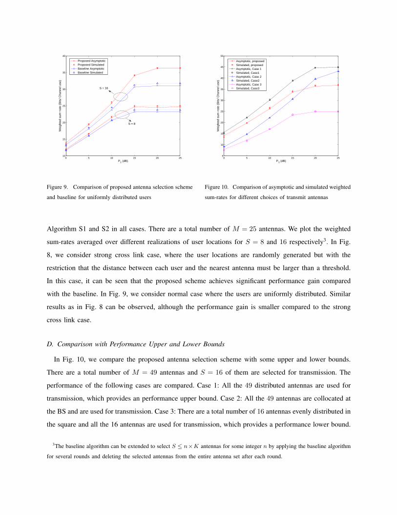
C. Performance Gain of the Proposed Scheme w.r.t. Baseline

In Fig. 8 and 9, we compare the performance of the proposed algorithm with the traditional antenna

selection baseline algorithm described in Section IV-D. The power allocation and ρ are optimized using

0 5 10 15 20 2510

15

20

25

30

35

40

PT (dB)

Wei

ghte

d su

m−

rate

(B

its/ C

hann

el u

se)

Proposed AsymptoticProposed SimulatedBaseline AsymptoticBaseline Simulated

S = 16

S = 8

Figure 9. Comparison of proposed antenna selection scheme

and baseline for uniformly distributed users

0 5 10 15 20 255

10

15

20

25

30

35

40

45

50

PT (dB)

Wei

ghte

d su

m−

rate

(B

its/ C

hann

el u

se)

Asymptotic, proposedSimulated, proposedAsymptotic, Case 1Simulated, Case1Asymptotic, Case 2Simulated, Case2Asymptotic, Case 3Simulated, Case3

Figure 10. Comparison of asymptotic and simulated weighted

sum-rates for different choices of transmit antennas

Algorithm S1 and S2 in all cases. There are a total number of M = 25 antennas. We plot the weighted

sum-rates averaged over different realizations of user locations for S = 8 and 16 respectively3. In Fig.

8, we consider strong cross link case, where the user locations are randomly generated but with the

restriction that the distance between each user and the nearest antenna must be larger than a threshold.

In this case, it can be seen that the proposed scheme achieves significant performance gain compared

with the baseline. In Fig. 9, we consider normal case where the users are uniformly distributed. Similar

results as in Fig. 8 can be observed, although the performance gain is smaller compared to the strong

cross link case.

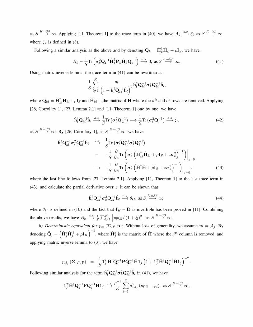
D. Comparison with Performance Upper and Lower Bounds

In Fig. 10, we compare the proposed antenna selection scheme with some upper and lower bounds.

There are a total number of M = 49 antennas and S = 16 of them are selected for transmission. The

performance of the following cases are compared. Case 1: All the 49 distributed antennas are used for

transmission, which provides an performance upper bound. Case 2: All the 49 antennas are collocated at

the BS and are used for transmission. Case 3: There are a total number of 16 antennas evenly distributed in

the square and all the 16 antennas are used for transmission, which provides a performance lower bound.

3The baseline algorithm can be extended to select S ≤ n×K antennas for some integer n by applying the baseline algorithm

for several rounds and deleting the selected antennas from the entire antenna set after each round.

We plot the weighted sum-rates averaged over different realizations of user locations versus sum power

constraint PT . The following advantages of the proposed antenna selection scheme can be observed. 1)

It achieves a weighted sum-rate close to the upper bound in Case 1, and higher than Case 2, while the

pilot training overhead is lower. 2) The performance is much better than Case 3 due to large antenna

gain. Note that as PT increases, the weighted sum-rate of the proposed scheme and Case 3 get saturated

earlier because in this two cases, the number of active antennas is smaller and the actual total transmit

power is smaller when PT is large.

VII. CONCLUSION

We consider downlink antenna selection problem in a large distributed MIMO network with M 1

geographically distributed antennas serving K users using RZF precoding. The objective is to maximize

the average weighted sum-rate under per antenna and sum power constraint by joint optimization of

antenna selection, regularization factor, and power allocation based on the knowledge of large scale

fading factors. The problem is a mixed combinatorial and non-convex problem. The objective and

constraints have no closed-form expressions. We first derive asymptotically accurate expressions for

average weighted sum-rate and transmit power. Then the joint optimization problem is decomposed

into simpler subproblems and efficient algorithms are proposed to solve them. For the special cases of

collocated antennas or collocated users, we obtain structural solution. We also show that the capacity of a

very large distributed MIMO network scales according to O(K ζ

2 logM)

, where ζ is the path loss factor.

Simulations show that the proposed antenna selection scheme provides a very good trade-off between

performance and CSI acquisition overhead.

APPENDIX

A. Proof of Lemma 1 and Lemma 2

a) Deterministic equivalent for γk (Σ, ρ,p): We first derive the deterministic equivalent for Ak and

Bk, then the deterministic equivalent for γk (Σ, ρ,p) follows immediately.

Ak can be rewritten as Ak = σ2kh†k

(H†kHk + ρIS

)−1hk, where σ2

k = diag(σ2kA1

, ...,σ2kAS), and

the elements of hk are i.i.d. complex random variables with zero mean, variance 1/S. Applying [26,

Corrolary 1] and [27, Lemma 2.1] one by one, we have

Aka.s−→ 1

STr(σ2k

(H†kHk + ρIS

)−1)

a.s−→ 1

STr(σ2k

(H†H + ρIS

)−1), (40)

as SK=Sβ−→ ∞. Applying [11, Theorem 1] to the trace term in (40), we have Ak

a.s−→ ξk as SK=Sβ−→ ∞,

where ξk is defined in (8).

Following a similar analysis as the above and by denoting Qk = H†kHk + ρIS , we have

Bk −1

STr(σ2kQ−1k H†kPkHkQ

−1k

)a.s−→ 0, as S

K=Sβ−→ ∞. (41)

Using matrix inverse lemma, the trace term in (41) can be rewritten as

1

S

K∑l 6=k

pl(1 + h†lQ

−1kl hl

)2 h†lQ−1kl σ

2kQ−1kl hl,

where Qkl = H†klHkl+ρIS and Hkl is the matrix of H where the kth and lth rows are removed. Applying

[26, Corrolary 1], [27, Lemma 2.1] and [11, Theorem 1] one by one, we have

h†lQ−1kl hl

a.s−→ 1

STr(σ2lQ−1kl

)−→ 1

STr(σ2lQ−1) a.s−→ ξl, (42)

as SK=Sβ−→ ∞. By [26, Corrolary 1], as S

K=Sβ−→ ∞, we have

h†lQ−1kl σ

2kQ−1kl hl

a.s−→ 1

STr(σ2lQ−1kl σ

2kQ−1kl

)= − 1

S

∂

∂zTr(σ2l

(H†klHkl + ρIS + zσ2

k

)−1)∣∣∣∣

z=0

−→ − 1

S

∂

∂zTr(σ2l

(H†H + ρIS + zσ2

k

)−1)∣∣∣∣

z=0

. (43)

where the last line follows from [27, Lemma 2.1]. Applying [11, Theorem 1] to the last trace term in

(43), and calculate the partial derivative over z, it can be shown that

h†lQ−1kl σ

2kQ−1kl hl

a.s−→ θkl, as SK=Sβ−→ ∞, (44)

where θkl is defined in (10) and the fact that IK −D is invertible has been proved in [11]. Combining

the above results, we have Bka.s−→ 1

S

∑Kl 6=k

[plθkl/ (1 + ξl)

2]

as SK=Sβ−→ ∞.

b) Deterministic equivalent for pm (Σ, ρ,p): Without loss of generality, we assume m = Aj . By

denoting Qj =(HcjH

c†j + ρIK

)−1, where Hc

j is the matrix of H where the jth column is removed, and

applying matrix inverse lemma to (3), we have

pAj (Σ, ρ,p) =1

S1Tj H†Q−1

j PQ−1j H1j

(1 + 1Tj H†Q−1

j H1j

)−2.

Following similar analysis for the term h†lQ−1kl σ

2kQ−1kl hl in (41), we have

1Tj H†Q−1j PQ−1

j H1ja.s−→ ρ−1

K

K∑i=1

σ2iAj (pivi − ϕi) , as S

K=Sβ−→ ∞,

where vi is defined in (12) and ϕi is defined in (15). Following similar analysis for the term h†lQ−1kl hl

in (42), we have

1Tj H†Q−1j H1j

a.s−→ 1

S

K∑i=1

σ2iAjvi, as S

K=Sβ−→ ∞.

Combining the above results, we show that as SK=Sβ−→ ∞, pm (Σ, ρ,p)

a.s−→ pm (Σ, ρ,p) in (16).

Finally, (ρIK + ∆−C)−1 is invertible because it is a diagonally dominant matrix. This completes

the proof of Lemma 1 and Lemma 2.

B. Calculation of the Derivative ∂I(A,ρ)∂ρ

For convenience, define two (S +K + 1)-dimensional vectors

pext =

p

0

, ~λext =

~λ

−~ν

.Define a (S +K + 1)×K matrix Rext ,

[RT ,−IK

]T . Define a vector e ∈ RK whose kth element is

ek =

K∑l=1

wlglk∑Ki=1 pi (A, ρ) ∂gli∂ρ(

gllpl (A, ρ) + Ωl

)2 −wl

∂glk∂ρ

gllpl (A, ρ) + Ωl

+

K∑l 6=k

(wl

∂glk∂ρ

Ωl

−wlglk

∑Ki 6=l pi (A, ρ) ∂gli∂ρ

Ω2l

).

Define a K ×K matrix Υ whose element at the kth row and lth column is

Υkl =

K∑l=1

−wlglkgln(1 +

∑Ki=1 glipi (A, ρ)

)2 +∑l 6=k,n

wlglkgln

Ω2l

.

Finally, define a (2K + S + 1)× (2K + S + 1) matrix

Υext =

Υ; −RText

diag(~λext

)Rext; diag (Rextp (A, ρ)− pext)

.Taking partial derivative of the equations in (31) with respect to ρ, we obtain the following linear

equations

Υext

∂p(A,ρ)∂ρ

∂~λext∂ρ

=

(∂R∂ρ

)T~λ+ e

−diag(~λext

)(∂Rext∂ρ

)Tp (A, ρ)

.Then we can obtain ∂p(A,ρ)

∂ρ by solving the above linear equations.

Define J1 =j : pAj (Σ, ρ, p (A, ρ)) < pAj

and K = k : pk (A, ρ) > 0. If pA (Σ, ρ, p (A, ρ)) <

PT , let J = J1∪S + 1, otherwise, let J = J1. Note that we have λj = 0, ∀j ∈ J and νk = 0, ∀k ∈ K

according to the KKT conditions. It can be verified that ∂λj∂ρ = 0, ∀j ∈ J and ∂νk∂ρ = 0, ∀k ∈ K. Therefore,

we can delete these |J | + |K| variables and the corresponding linear equations whose index i satisfies

i−K ∈ J or i− S −K − 1 ∈ K. The remaining 2K + S + 1− |J | − |K| variables can be determined

by the remaining linear equations. After obtaining ∂p(A,ρ)∂ρ , the derivative ∂I(A,ρ)

∂ρ can be calculated using

(32).

To complete the calculation of ∂I(A,ρ)∂ρ , we still need to obtain ∂gkl

∂ρ , ∀k, l, and ∂R∂ρ . The following

Lemma are useful and can be proved by a direct calculation.

Lemma 3 (Derivatives of the intermediate variables): For the intermediate variables ~θk, v, ∆ and C

defined in Lemma 1 and Lemma 2, the partial derivatives of them with respective to ρ are given below.∂~θk∂ρ

= (IK −D)−1

(∂dk∂ρ

+∂D

∂ρ~θk

), ∀k, (45)

where ∂dk∂ρ is given by

∂dkl∂ρ

= − 2

S

∑m∈A

[σ2kmσ

2lm

(1− 1

S

K∑i=1

σ2imφi

(1 + ξi)2

)/f3m

(~ξ)]

, ∀l,

and ∂D∂ρ is given by

∂Dln

∂ρ=

1

S2

∑m∈A

[2σ2

lmσ2nm

(1 + ξn)2

[1

S

K∑i=1

σ2im

1 + ξi

(φi

1 + ξi− φn

1 + ξn

)− 1− ρφn

1 + ξn

]/f3m

(~ξ)]

.

∂Cln∂ρ

=1

S

∑m∈A

[1

Sσ2lmσ

2nm

∂vl∂ρ

/ψ2m (v)− 2

Sσ2lmσ

2nmvl

1

S

K∑i=1

σ2im

∂vi∂ρ

/ψ3m (v)

], ∀l, n, (46)

∂4l

∂ρ= − 1

S

∑m∈A

[σ2lm

1

S

K∑i=1

σ2im

∂vi∂ρ

/ψ2m (v)

], ∀l, (47)

∂v

∂ρ= − (ρIK + ∆−C)−1 v, (48)

Using Lemma 3, ∂gkl∂ρ , ∀k, l, and ∂R

∂ρ can be obtained by a direct calculation as follows.

∂gkk∂ρ

=2ξk

∂ξk∂ρ

(1 + ξk)3 , ∀k,

∂gkl∂ρ

=

∂θkl∂ρ

S (1 + ξl)2 (1 + ξk)

2 −2θkl

[∂ξl∂ρ (1 + ξk) + ∂ξk

∂ρ (1 + ξl)]

S (1 + ξl)3 (1 + ξk)

3 , ∀k 6= l,

where ∂ξk∂ρ = φk, ∀k is defined in (9), ~θk = [θk1, ..., θkK ]T , ∀k is defined in (10) and ∂~θk

∂ρ is given in

(45). To calculate ∂R∂ρ , we first obtain ∂R

∂ρ as

∂Rkj∂ρ

= −σ2kAjρ

−1

S2

[ρ−1/ψ2

Aj (v) +2

S

K∑i=1

σ2iAj

∂vi∂ρ

/ψ3Aj (v)

], ∀k, j.

where ∂vi∂ρ , ∀i is given in (48). Then we obtain ∂R

∂ρ as

∂Rkk∂ρ

=1

S

∑m∈A

σ2km

∂vk∂ρ

+ σ2km

1

S

K∑i 6=k

σ2im

(vk∂vi∂ρ

+ vi∂vk∂ρ

) /ψ2m (v)

−

2σ2kmvk

1 +1

S

K∑i 6=k

σ2imvi

1

S

K∑i=1

σ2im

∂vi∂ρ

/ψ3m (v)

, ∀k,∂Rkl∂ρ

= − 1

S

∑m∈A

[σ2kmσ

2lm

1

S

(vl∂vk∂ρ

+ vk∂vl∂ρ

)/ψ2

m (v)− 2

Sσ2kmσ

2lmvkvl

1

S

K∑i=1

σ2im

∂vi∂ρ

/ψ3m (v)

], ∀k 6= l.

Finally, ∂R∂ρ =

[IS , 1

]T∂R∂ρ and ∂R

∂ρ is given by

∂R

∂ρ=

(∂R

∂ρ

)T (V − (ρIK + ∆−C)−1 R

)+ RT

(∂V

∂ρ− (ρIK + ∆−C)−1 ∂R

∂ρ

)+RT

(IK +

∂∆

∂ρ− ∂C

∂ρ

)(ρIK + ∆−C)−2 R,

where ∂C∂ρ and ∂∆

∂ρ are given in (46) and (47) respectively, and ∂V∂ρ = diag

(∂v1∂ρ , ...,

∂vK∂ρ

).

C. Proof of Theorem 5

When P′

T is large enough, all users will be allocated with positive power. In this case, the SINR of

user k under power allocation in (36) is given by

γk (ρ,p∗ (A, ρ)) =Swk

(1 + σ2

k1u)2σ2k1

(2ρuP

′

T + (β − 1)P′

T + 1S

∑Kl=1

1σ2l1

)(∑K

l=1wl

)(σ2k1P

′

T +(1 + σ2

k1u)2) − 1, (49)

and the objective of P2 (A) is given by I (A, ρ,p∗ (A, ρ)) =∑K

k=1wklog (1 + γk (ρ,p∗ (A, ρ))). For

any k, it can be shown that the solution ρk of ∂∂ρ γk (ρ,p∗ (A, ρ)) = 0 must satisfy ρk = O

(1P′T

). Since

the optimal regularization factor ρ∗ must satisfy minkρk ≤ ρ∗ ≤ max

kρk, we have ρ∗ = O

(1P′T

). To prove

the second result, it can be verified that ∂2

∂2ρ γk (ρ,p∗ (A, ρ)) < 0 and thus γk (ρ,p∗ (A, ρ)) is concave

when ρ is small enough. Since I (A, ρ,p∗ (A, ρ)) is a concave increasing function of γk (ρ,p∗ (A, ρ)),

I (A, ρ,p∗ (A, ρ)) must be a concave function of ρ [22].

D. Proof of Theorem 7

We first derive a lower bound for the probability that the minimum distance rmin between any two

users is larger than a certain value r0: Pr (rmin ≥ r0). Let dukl denote the distance between user k and

user l. We have

Pr (rmin ≥ r0) = 1− Pr(

minl 6=k

dukl ≤ r0, ∃k ∈ 1, ...,K)

≥ 1−K∑k=1

Pr(

minl 6=k

dukl ≤ r0

)= 1−KPr

(minl 6=1

du1l ≤ r0

)= 1−K

[1− (Pr (du12 ≥ r0))K−1

]≥ 1−K

[1−

(1− πr2

0

R2c

)K−1],

where the second inequality follows from the union bound and the last inequality holds because Pr (du12 ≥ r0)

≥ 1− πr20R2c

.

Then we use the path loss model to transfer the probability Pr (rmin ≥ r0) to the probability Pr (η > η0)

in (39). Note that for any k, we have minm

rkm ≤√

2Rc2√M

, and maxlrkml

≥ rmin −√

2Rc2√M

. Hence η ≥(rmin/

(√2Rc

2√M

)− 1)ζ

and

Pr (η > η0) ≥ Pr

((rmin/

(√2Rc

2√M

)− 1

)ζ> η0

)

= Pr(rmin >

√2Rc

2√M

(η

1/ζ0 + 1

))≥ 1−K

[1−

(1− π

(η

1/ζ0 + 1

)2/ (2M)

)K−1].

Finally, we prove the capacity scaling by deriving an upper and a lower bound for the sum-rate. The

following lemma follows directly from Assumption 3 and is useful for deriving the upper bound.

Lemma 4: For any ε > 0, as M →∞ with K,S fixed, we have

Pr(

mink,m

rkm ≤M−1

2−ε)

=πM−2ε

R2c

→ 0,

and thus

Pr(gdk > G0M

ζ

2+ε)→ 0.

Let PUT = max(PT ,max

m∈ASpm

)and let XS denote a random variable with χ2 (2S) distribution.

Assuming that each user is severed by S antennas without interference from other users, we obtain an

upper bound for average sum-rate as follows:

Cs ≤ KE[log(

1 + PUT gdkXS

)]≤ Klog

(1 + PUT g

dkE [XS ]

). (50)

Combining (50) with Lemma 4, we prove that Cs ≤ O(K(ζ2 + ε

)logM

)holds almost surely as

M →∞ with K,S fixed.

Furthermore, it follows from the lower bound provided in Appendix E that Cs ≥ O(K(ζ2 − ε

)logM

).

This completes the proof of Theorem 7.

E. Proof of Corollary 1

Due to (39) in Theorem 7, the step 1 in Algorithm S3 will almost surely select a set of antennas

A, |A| = K such that each user has strong direct-link with one of the selected K antennas and weak

cross-links with other selected antennas for large M/K. Assume that each selected antenna only severs

the nearest user, and assume equal power allocation for each user, i.e., pk = min(PT /K, min

m∈Apm

), k =

1, ...,K. Let Xm denote a random variable with χ2 (2m) distribution. Let η0 = Mζ

2−ε1 in (39). Then

using (39) and the fact that gdk ≥ G0

(√2Rc

2√M

)−ζ, we can show that as M → ∞ with K,S fixed, the

average sum-rate IA is almost surely lower bounded by

IAa.s≥ KE

log

1 +p1G0

(√2Rc

2√M

)−ζX1

1 + p1M− ζ

2+ε1G0

(√2Rc

2√M

)−ζXK−1

, (51)

where X1 and XK−1 are independent. Choose B1, B2 > 0 such that Pr (X1 ≥ B1) Pr (XK−1 ≤ B2) ≥

1− ε2. Then as M →∞ with K,S fixed, it follows from (51) that

IAa.s≥ K (1− ε2) log

1 +p1G0

(√2Rc

2√M

)−ζB1

1 + p1M− ζ

2+ε1G0

(√2Rc

2√M

)−ζB2

= O

(K (1− ε2)

(ζ

2− ε1

)logM

).

Choose ε1, ε2 such that ε1 + ζ2ε2 − ε1ε2 = ε. Then we have IA

a.s≥ O

(K(ζ2 − ε

)logM

)as M → ∞

with K,S fixed. The rest steps in S3 only increase the sum-rate by a constant. This completes the proof.

REFERENCES

[1] T. Marzetta, “How much training is required for multiuser MIMO?” Fortieth Asilomar Conf. on Signals, Systems, and

Computers, Pacific Grove, CA, pp. 359 – 363, Oct. 2006.

[2] F. Rusek, D. Persson, B. K. Lau, E. G. Larsson, O. Edfors, F. Tufvesson, and T. L. Marzetta, “Scaling up MIMO:

Opportunities and challenges with very large arrays,” to appear in IEEE Signal Processing Magazine, 2012. [Online].

Available: http://arxiv.org/abs/1201.3210

[3] A. Moustakas, S. Simon, and A. Sengupta, “Mimo capacity through correlated channels in the presence of correlated

interferers and noise: a (not so) large n analysis,” IEEE Trans. Inf. Theory, vol. 49, no. 10, pp. 2545 – 2561, oct. 2003.

[4] A. Tulino, A. Lozano, and S. Verdu, “Impact of antenna correlation on the capacity of multiantenna channels,” IEEE Trans.

Inf. Theory, vol. 51, no. 7, pp. 2491 – 2509, Jul. 2005.

[5] B. Hochwald and S. Vishwanath, “Space-time multiple access: Linear growth in the sum rate,” Proc. Allerton Conf. on

Commun., Control, and Computing, vol. 40, no. 1, pp. 387 – 396, 2002.

[6] Y.-C. Liang, S. Sun, and C. K. Ho, “Block-iterative generalized decision feedback equalizers for large MIMO systems:

algorithm design and asymptotic performance analysis,” IEEE Trans. Signal Processing, vol. 54, no. 6, pp. 2035 – 2048,

Jun. 2006.

[7] K. Vishnu Vardhan, S. Mohammed, A. Chockalingam, and B. Sundar Rajan, “A low-complexity detector for large MIMO

systems and multicarrier cdma systems,” IEEE J. Select. Areas Commun., vol. 26, no. 3, pp. 473 – 485, april 2008.

[8] T. Marzetta, “Noncooperative cellular wireless with unlimited numbers of base station antennas,” IEEE Trans. Wireless

Commun., vol. 9, no. 11, pp. 3590 – 3600, Nov. 2010.

[9] J. Jose, A. Ashikhmin, T. Marzetta, and S. Vishwanath, “Pilot contamination and precoding in multi-cell TDD systems,”

IEEE Trans. Wireless Commun., vol. 10, no. 8, pp. 2640 – 2651, August 2011.

[10] R. Muharar and J. Evans, “Downlink beamforming with transmit-side channel correlation: A large system analysis,” in

Proc. IEEE ICC 2011, pp. 1 – 5, Jun 2011.

[11] S. Wagner, R. Couillet, M. Debbah, and D. T. M. Slock, “Large system analysis of linear precoding in correlated

MISO broadcast channels under limited feedback,” submitted to IEEE Trans. Inf. Theory. [Online]. Available:

http://arxiv.org/abs/0906.3682

[12] C. Peel, B. Hochwald, and A. Swindlehurst, “A vector-perturbation technique for near-capacity multiantenna multiuser

communication-part I: channel inversion and regularization,” IEEE Trans. Commun., vol. 53, no. 1, pp. 195 – 202, Jan.

2005.

[13] J. Hoydis, S. ten Brink, and M. Debbah, “Massive MIMO in UL/DL cellular systems: How many antennas do we need?”

submitted to IEEE J. Select. Areas Commun., Special Issue on "Large-Scale Multiple Antenna Wireless Systems", 2011.

[14] Huawei, “Cloud RAN introduction,” The 4th CJK International Workshop, Sep. 2011.

[15] R. Zakhour and S. V. Hanly, “Base station cooperation on the downlink: Large system analysis,” submitted to IEEE

Trans. Info. Theory, Jun. 2010. [Online]. Available: http://arxiv.org/abs/1006.3360

[16] R. Chen, J. Andrews, and R. Heath, “Efficient transmit antenna selection for multiuser MIMO systems with block

diagonalization,” in Proc. IEEE GLOBECOM 2007, pp. 3499 –3503, Nov. 2007.

[17] M. Mohaisen and K. Chang, “On transmit antenna selection for multiuser MIMO systems with dirty paper coding,” in

Proc. IEEE PIMRC 2009, pp. 3074 –3078, Sep. 2009.

[18] R. Irmer, H. Droste, P. Marsch, M. Grieger, G. Fettweis, S. Brueck, H.-P. Mayer, L. Thiele, and V. Jungnickel, “Coordinated

multipoint: Concepts, performance, and field trial results,” IEEE Communications Magazine, vol. 49, no. 2, pp. 102 –111,

february 2011.

[19] B. Chalise, L. Haering, and A. Czylwik, “Robust uplink to downlink spatial covariance matrix transformation for downlink

beamforming,” in Proc. IEEE ICC 2004, pp. 3010 – 3014, Jun. 2004.

[20] B. Hochwald and T. Maretta, “Adapting a downlink array from uplink measurements,” IEEE Trans. Signal Processing,

vol. 49, no. 3, pp. 642 –653, Mar 2001.

[21] J. Hoydis, R. Couillet, and M. Debbah, “Random beamforming over correlated fading channels,” submitted to IEEE

Trans. Info. Theory, 2011. [Online]. Available: http://arxiv.org/abs/1105.0569

[22] S. Boyd and L. Vandenberghe, Convex Optimization. Cambridge University Press, 2004.

[23] A. Liu, V. K. N. Lau, and Y. Liu, “Local dual method for optimization of parallel MIMO B-MAC interference networks

under multiple linear constraints,” submitted to IEEE Trans. Signal Processing, Sep. 2011; revised Apr. 2012. [Online].

Available: http://www.ee.ust.hk/~eeknlau/HKUST-Office-HomePage/Publications.html

[24] D. G. Luenberger and Y. Ye, Linear and Nonlinear Programming, 3rd ed. New York: Springer, 2008.

[25] C. Shi, R. A. Berry, and M. L. Honig, “Monotonic convergence of distributed interference pricing in wireless networks,”

in Proc. IEEE ISIT, Seoul, Korea, June 2009.

[26] J. Evans and D. Tse, “Large system performance of linear multiuser receivers in multipath fading channels,” IEEE Trans.

Inf. Theory, vol. 46, no. 6, pp. 2059 –2078, sep 2000.

[27] Z. Bai and J. Silverstein, “On the signal-to-interference ratio of CDMA systems in wireless communications,” Ann. Appl.

Probab., vol. 17, no. 1, p. 81, 2007.