TECHNICAL REPORT RD-RE-87-3

DIAGNOSTIC PARAMETER DETERMINATIONFOR A CLASS OF THREE-PARAMETER

CO PROBABILITY DISTRIBUTIONS0N

V) S. H. Lehnigk and H. P. Dudel0 Research DirectorateN Research, Development, & Engineering Center

JULY 1987

fedstce A3r5en8, Albama 98-5000

. Appruved for public release; distribution unlimited.

PTICI t 1989o., . . .., -

.4

SM, FORM 1021, 1 AUG 85 PREVIOUS EDITION IS OBSOLETE 89 2 6 087 i

DISPOSITION INSTRUCTIONS

DESTROY THIS REPORT WHEN IT IS NO LONGER NEEDED. DO NOTRETURN IT TO THE ORIGINATOR.

DISCLAIMER

THE FINDINGS IN THIS REPORT ARE NOT TO BE CONSTRUED AS AN

OFFICIAL DEPARTMENT OF THE ARMY POSITION UNLESS SO DESIG-NATED BY OTHER AUTHORIZED DOCUMENTS.

TRADE NAMES

USE OF TRADE NAMES OR MANUFACTURERS IN THIS REPORT DOESNOT CONSTITUTE AN OFFICIAL INDORSEMENT OR APPROVAL OFTHE USE OF SUCH COMMERCIAL HARDWARE OR SOFTWARE.

m a I II II

U11CLASSIFIEDSECURITY CLASSIFICATION OF THIS PAGE

REPORT DOCUMENTATION PAGE F"OrNapmved"_________________________________________Eixp Darto Jun 30 1986

la REPORT SECURITY CLASSIFICATION lb. RESTRICTIVE MARKINGSUNCLASSIFIED

2a SECURITY CLASSIFICATION AUTHORITY 3, DISTRIBUTION JAVAILABILITY OF REPORTApproved for public release; distribution

2b. DECLASSIFICATION IDOWNGRAOING SCH4EDULE unlimited.

4. PERFORMING ORGANIZATION REPORT NUMBER(S) S. MONITORING ORGANIZATION REPORT NUMBER(S)

RD- RE 87-3

6a. NAME OF PERFORMING ORGANIZATION 6b. OFFICE SYMBOL 7a. NAME OF MONITORING ORGANIZATIONResearch Directorate ifplcbeRD&E Center IAMSMI-RD-RE-OP6C. ADDRESS (City. State, and ZIP Code) 7b. ADDRESS (City. State, and ZIP Code)Commander, US Army Missile CommandATTN: AMSMI-RD-RE-OPRedstone Arsenal, AL 35898-5248 ______________________

84. NAME OF FUNDING / SPONSORING 8b. OFFICE SYMOL 9. PROCUREMENT INSTRUMENT IDENTIFICATION NUMBERORGANIZATION #IfA9110-1111)

Sk. ADDRESS (City. State, and ZIP Code) 10. SOURCE OF FUNDING NUMSERSPROGRAM .I PROJECT I TASK I WORK UNITELEMENT NO. O. NO rCESSION NO

11. TITLE (Include Secunty Clification)Diagnostic Parameter Determination for a Class of Three-ParameterProbability Distributions (U)

?2. PERSONAL AUTHOR(S)

S. H. Lehniak and H. P. Dudel13a. TYPE OF REPORT 13b. TIME COVERED 14. DATE OF REPORT (Yo"., Month, Day) IS. PAGE COUNTFinal Technical IFROM_____ TO 61 July 1987 4

16. SUPPLEMENTARY NOTATION

17. COSATI CODES 1S. SUBJECT TERMS (Continue an rovrSe it neceUaiY and iadintifr by bslock number)FIELD GROUP SUB-GROUP Hyper-Gammna Distribution, Three Parameters, Density

Estimation, Approximation of Cumulative Distribution

19. ABSTRACT (Continue on rgwvem if riecuflary and identify by block number)

The problem of parameter estimation of the non-shifted hyper-Gamma class is being con-sidered. The approach is based on an applicability criterion which provides the oppor-tunity to determine the parameters by means of three equations derived from the first andsecond moments and an analytical approximation of the logarithm of the cumulative distri-bution function. The parameter estimation process requires the iterative solution of twoequations. Examples are given to verify the efficiency of the proposed parameter deter-mination method. Recently obtained results on maximum-likelihood parameter estimationfor the hyper-Gamma class nay turn out to be practically more reliable than those presentedin this report, especially for non-smooth data.

20. DISTRIBUTION / AVAILABILITY OF ABSTRACT 21 ABSTRACT SECURITY CLASSIFICATION13 UNCLASSIFIECWUN4LIMITED (3 SAME AS RPT. C3 oTic USERS UNCLASSIFIED

22a. NAME OF RESPONSIBLE INDIVIDUAL 22b TELEPHONE (include Area Code) 22c. OFFICE SYMBOL

i". ehnik- -176 AMSMI-RD-RD-OPDO FORM 1473, 54 MAR 83 APR edition may be used until exhausted. SECURITY CLASSIFICATIONOF THIS PAGE_

All other edition% are obsolete. UNCLASSIFIED

i/(ii blank)

TABLE OF CONTENTS

Page

I. INTRODUCTION ....................................................... I

II. NOTATIONS AND FORMULAS ............................................ 4

III. THE APPLICABILITY CRITERION ....................................... 6

IV. DETERMINATION OF THE PARAMETERS ................................... 8

V. THE ITERATION PROCESS ............................................. 13

VI. EXAMPLES ....................................................... 15

REFERENCES ........................................................... 26

APPENDIX A. THE EQUATION h(R,a) 0 ................................. A-i

APPENDIX B. APPROXIMATION OF v(u) by v*(u) ........................... B-i

APPENDIX C. THE COEFFICIENT a AS A FUNCTION OF R .................... C-I

APPENDIX D. CONVERGENCE OF THE ITERATION PROCESS .................... D-I

iij/(iv blank)

LIST OF TABLES

Figure Title Page

1 Empirical Example #3 - Absolute Frequencies ..................... 9

2 Empirical Example #3 - Relative Frequencies .................... 10

3 SYNEX #8: Exponential Weibull Distribution

(B-1, P-0, Beta-1) ........................................... 16

4 SYNEX #9: Weibull Distribution (B-i, P-il, Beta-2) ..............17

5 SYNEX #10: Weibull Distribution (B=2, P--2, Beta-3) .............18

6 SYNEX .#10: Weibull Distribution (B-2, Pin12, Beta-3) .............19

7 SYNEX #11: Weibull Distribution (B-5, P-0.5, Beta-O.5) ..........20

8 Empirical Example #3 .......................................... 21

Acce-z Por

FV--NT 7--

vI(vi. blank)

SUMMARY

The application of a class of continuous, one-sided, three-parameterprobability distributions is being considered. The parameters represent scaleand initial and terminal shape of the associated probability density function.The class contains as special cases (for specific numerical values of theshape parameters) the following well-known distributions: Gauss, Welbull,exponential, Rayleigh, Gamma, chi-square, Maxwell, and Wien. The objective isto present and discuss a parameter determination technique which uses cumula-tive frequency data. The approach is based on an applicability criterion forthe considered distribution class which provides the opportunity to determinethe parameter values by means of three equations derived from the first andsecond moments, and an analytical approximation of the logarithm of the cumu-lative distribution function. Since the scale-parameter can be eliminated,the parameter determination process requires the Iterative solution on a per-sonal computer (PC) of only two equations. Convergence of the iteration pro-cess provides the ultimate practical justification for the applicability ofthe considered distribution class relative to given empirical data. Examplesare given to verify the efficiency of the proposed parameter determinationmethod.

vii/(viii blank)

I. INTRODUCTION

The objective is to revitalize interest in the application of a class ofprobability distributions which had been designated a generalized Gammadistribution by various authors [1, 2, 3, 4, and 51. This class representsthree-parameter, continuous, one-sided distributions which may be defined interms of the cumulative distribution function (cdf)

F r((1 p)F) y((-p)S 1,FS), F = xb-1, x > 0, (W)F(x)=

0, x < 0,

with parameters b, p, and R, r(y) and y(a,y) being the Gamma function and theincomplete Gamma function (with lower integration limit zero), respectively.

Apparently, this class of distributions was introduced originally byL. Amoroso [6]. Various aspects of it received attention in fairly recentpublications [7, 8]. These papers refer to the close connection of the class(*), via the associated probability density function (pdf), with a class ofparabolic differential equations (generalized Feller equation). They alsoestablish a connection with the underlying dynamical diffusion process. Inthis context the publication [9, Sec. 7] may be of particular interest.

The probability density function (pdf) class associated with the cdf class(*) is given by

dF(x) b- -P exp -F, P = xb- 1 , x > 0,f(x) - dx 0

10, x < 0. (1)

The expression for f(x) clearly demonstrates the meaning of the parametersb, p, and R. The parameter b > 0 represents scale, p < I represents initialshape (for small values of x > 0) and 8 > 0 represents terminal shape (forlarge values of x).

A shift parameter xo may be introduced by replacing x by x-xo , x > xo .That will not be done here, however, since only distributions of the three-parameter type (*), (I), are of interest. To partially lift the restrictionson p and 8, one may replace the independent variable x by, say, y-1 , y > 0being a new independent variable; however, this possibility will not be offurther concern here. Another remark concerns a notational change relative tothe earlier papers (7, 8, 9]. The parameter A which appeared there has beenreplaced by A - I - X.

• 1

The reason for the designation of p and 8 as initial and terminal shapeparameters, respectively, is evident. For large values of x, the exponentialfunction in (1) is the dominating factor and, consequently, the shape of thepdf curve or, more precisely, its rate of decay, for large values of x isdetermined by $. In any case, f(x) + 0 as x + + -. Since the exponentialfunction approaches unity as x + 0, the initial shape of the pdf curve isdetermined by p. If 0 < p < 1, f(x) + + - as x + 0 so that, in this case, aJ-shaped distribution is being dealt with. If p = 0, f(x) + R/br(br(R-1 )); thedistribution is of the half bell-shaped type (purely exponential). Finally,if p < 0, f(x) + 0 as x + 0. The distrib'tion is hump-shaped, the pdf havinga unique maximum at the point xm - b(-pR-1)l/B.

For particular values of the shape parameters, the class of distributionscharacterized by (*) contains a number of special cases well-known in sta-tistics and statistical physics. The major ones are: [2, 7, 10]:

Gauss (p - 0, 8 - 2),Weibull (p l 1 - 8 < 1),exponential (p - I - 6 - 0),Rayleigh (p = 1 - 8 = - 1),Gamma (p < 1, 6 - I),chi-square (p - (2 - v)/2 < 1, 8 - 1),Maxwell (p - - 2, 8 = 2, x - vto, b - (2kT/m)l/2to), andWien (p - - 3, 8 = 1, x - 2rcwo-2w, b = 2ncw- 2kT*l1 .

Apparently, application of the distribution class (*) has been severelylimited, although various attempts have been made, [1, 2, 3, 4, and II] forthe special cases of Gamma and Weibull to formalize and standardize the para-meter estimation process. In fact, the distribution class (*), has not beenused as extensively in every day statistical practice as it should be. Themain reason for this state of affairs is most likely attributed to com-putational intensity and possibly to convergence problems arising in thenumerical solution of the associated maximum-likelihood equations. Thisreport will not deal further with questions related to the maximum-likelihoodapproach. This will be done elsewhere in a separate publication.

From an application point of view, to revitalize interest in the distri-bution class (*) means to provide a practically useful, efficient, and com-putationally economical technique for the determination of the three unknownparameters b, p, and 8 relative to given frequency data. Practical usefulnessimplies the notion of a criterion being involved whose satisfaction can beverified in the application of the technique. The parameter determinationtechnique that is being proposed here does involve such a criterion. It isbased on an applicability criterion, announced already [71, which is charac-teristic for the distribution class (*). This criterion, which will be pre-sented in Section II, recognizes the fact that the logarithm of the cdf,is asymptotically linear in log x as x approaches zero from above. Thistypical property of the class (*), can be exploited to establish one equationin the three unknowns b, p, and 6, which encompasses the cumulative frequencydata. Two more equations in the three unknowns are obtained from the firstand second moments which can be numerically determined from the relative fre-quency data. Since the scale parameter b can easily be eliminated by means ofthe first moment, two equations are eventually left in the unknowns p and 8.

2

The equation resulting from the log cdf function is too complicated tobe used directly. Therefore, it will be replaced by a simpler approximatingfunction which will subsequently be used for a least squares fit of the givenlog cdf points. The quality of this approximation will be discussed inAppendixes B and C.

The solution of the two final equations for the two unknown parameters pand A proceeds by iteration (Section V). Convergence of the iteration processprovides the ultimate practical justification for the application of thedistribution class (*), relative to given empirical data (Appendix D).

A number of examples are presented in Section VI. These are "synthetic"examples in the sense that their parameter values are known in advance andthen reconstructed by means of the proposed parameter determination method. Aquality test is immediately available by means of comparison of the originaland the calculated parameter values. One empirical example has been includedfor purposes of exposition and demonstration. No attempt will be made in thisreport to do a goodness-of-fit test. This will be left to another publicationwhich will deal exclusively with empirical examples.

While work on this project was in progress and during its publicationphase, parallel efforts on maximum-likelihood density estimation fQr thehyper-Gamma class have led to essential new results [14] which cover both thethree- and four-parameter cases. Although computer programming via themaximum-likelihood approach is more complex than that required by the tech-nique presented in this report, maximum-likelihood density estimation may bepreferable in practice. Nevertheless, the method presented here leads quicklyto approximate parameter values which may be used as initial values inmaximum-likelihood estimations.

3

II. NOTATIONS AND FORMULAS

In statistical practice, empirical, data are normally given in terms ofabsolute frequencies, fa, relative to a finite number m of class intervals,[xv-l, xv)(v - 1, ..., m). The intervals are assumed to be of equal length,d - x. - xV_], so that xv - vd, and xo = 0.

The (piecewlse constant) absolute frequency function fa(x), xE[O, xm),is defined as fa(x) - fa(Xv-1) for xE[xvl, xv). A relative frequency

function, fr(x), xE[O,xm) can now be defined as fr(x) - N-lfa(x), N beingthe total number of observations, i.e.,

m

N -Ifa(X,).

V-1

With fr(x) one associates the (empirical) 'pdf f(x) - d-lfr(x), xE[O, xx). Amajor problem in statistical analysis arises in the attempt to construct acontinuous analogue of a given (piecewise constant) empirical pdf. The mainobjective of the work to be presented in this report deals with a new approachto the solution of this problem within the class of distributions (*).

The (empirical) cdf associated with given frequency data is defined as acontinuous and piecewise linear function F(x) with functional values at x - 0and at the interval endpoints given by

F(O) - 0,

V VF(xv) 1 : f(x,-I)d E Y fr(xul)(v - 1, ... , m). (2)

The set of m class intervals, [xv_1, xv), x0 U 0, x - vd (v - 1, ... m)together with the cdf values, F(x,), as defined in (2), shall be called anempicical data set.

The (theoretical) moments of the distribution class (*) are given by theformula

MV xvf(x)dx - bv r((v+l-p)R-l) (v - 0, 1, 2, ... ) (3)r ( ( l-p ) S- 1), ,,

0

f(x) given by (1), Mo - 1, MI U u being the mean value, and M2 being the meansquare value.

Observe the important inequality

o< i (4)M2

!4

which follows from

0 < f (x-u)2f(x)dx - M2 - U2 .

0

Replacement of f(x) in (3) by the empirical pdf yields the (empirical)first and second moments,

m

Ml - d E fr(xv)(v - 1/2), (5)

v-I

m

M2 - d2 E fr(x,)(v(v 1) + 1/3). (6)

v-1

5

III. THE APPLICABILITY CRITERION

Now return to the cdf class, F(x), given in (*). By means of the defi-nition of the incomplete Gamma function y(a, y) in terms of the degeneratehyper-geometric function 4(.,.;.) (12; 9.236.4] the nontrivial part of F(x)can be represented in the form

F(x) 0p p IP ((l-p)wl, I + (l-p)g-1 ; -

- xb-1, x>O.

This allows a useful expression for the logarithm of F(x) to be obtained:

log F(x) = - log r(l +(l-p)8 - I) + (l-p)log xb- I

+ log D ((l-p)8 -1 , 1 + (l-p)8- 1; - (xb-1 )8). (7)

The independent variable transformation x - Mly is carried out. The reasonfor this transformation is that, for a given empirical data set, all intervalendpoints x. M vd with x. < M1 will be transformed into points Yv with0 < yv < 1, so that the corresponding numbers u. - log yv - log x MI- I willbe negative. (In some cases where there are only a few points x. < MI, it maybe better to transform x into y by means of a factor K, M1 < K < xm. In anycase, from a practical point of view, as will be seen shortly, it is essentialto have "sufficiently" many numbers uV = log yV - log xV - I with uV < 0.)With log y = u and log F(x) = log F(MIy) - log F(Mleu - v(u), so that log xb- l - log yMlb

-I - u - log MI-1 , the functional relation

v(u) = (l-p)u - log r(l+(l-p)q-i)-(l-p) log Ml-lb

+ log o ((1-p)8 -1 , 1 +(1-p)8-1 ; - (Mjb-lea) ) (8)

is obtained from (7). The function 0 is represented as a power series in itslast argument with constant term equal to unity. Therefore, as x 4 0, i.e.,as y + 0, which means as u + - -, log 0 + 0. (For the argument of ( in (8)the series is alternating and, hence, 0 < D < 1.) Consequently, the functionv(u) given in (8) is asymptotically linear in u as u + - -. In other words,

v(u) - va(u) = (l-p)u-log r(l+(l-p)8- ) - (1-p) log Ml-lb, u 4. - -.

This asymptotic linearity property may also be expressed by saying that, asu 4 - -, the graph of the function v(u) approaches the (straight line) asymp-tote determined by the equation

va(u) -(1-p)u - log f(l+(1-p)9 -1 ) - (l-p) log Ml-lb.

6

Here and In (8) the scale parameter b may be eliminated by weans of the firstmoment, using (3) for v - 1,

b = Ml r(-P)8-1),r((2-p)8 - 1)

which leads to

va(u) = (l-p)u-log(l-p)R-1-(2-p)logr((l-p)%-l)

+(l-p)logr((2-p)R-1). (9)

Obviously, the graph of the function v(u) has a second asymptote, namely theline v = 0 four u + = -. This one, however, is of no further interest.

Based on the asymptotic linearity property of the function v(u), one canformulate the following applicability criterion which has been announcedalready in [7]:

A distribution function F(x) of the class (*) may be considered as acandidate for a data fit if the logarithmic plot of a given set of empirical

data, i.e., the plot of the points P , - (u ,,vJ) ul, log x -,K1, Mi < K < xm,v,- log F(x,,) (v = 1, ..., m), indicates the existence of an asymptote as u

It is essential to observe that the initial shape parameter p of amember of the distribution class (*) is uniquely determined by the directionangle 9 of the asymptote of the graph of the function v(u). According to (8)and (9), i-p - tan e. This fact will be exploited in the parameter deter-mination method.

7

IV. DETERMINATION OF THE PARAMETERS

This section presents the general outline of the proposed parameterdetermination method relative to the distribution class (*). The actual com-putational procedure will be established in Section V.

Determination of the parameters b, p, and 8 relative to a given empiricaldata set requires the solution of three simultaneous equations. For nota-tional convenience p is replaced by 1-a. Since the scale parameter b can beexpressed uniquely in terms of the two shape parameters by means of the firstmoment (3), it is actually necessary to have only two equations involving thetwo shape parameters. One such equation can be obtained from the secondmoment upon elimination of b. It is of the form

h(S,a) - r2 I17 - Ar 2) r OA -- M2 (10)

in which, according to (4), 0 < A < I. A second equation, g(R,a) - 0, followsfrom the function v(u) given in (8) if u - 0 and b is eliminated.

Unfortunately, the second equation is unpleasant from a computationalpoint of view. It is desirable, therefore, from a practical standpoint, toreplace it by some other equation which can more easily be handled.

To achieve this objective, an approximating function v*(u) is used forthe function v(u) with the fact in mind that the asymptote of the graph ofv(u) determines the initial shape parameter uniquely. For v*(u) the function

v*(u) - au + o(eSu-l) + v(O), a - 1-p (11)

is chosen.

There are several reasons for this choice of v*(u):

(1) The graph of v*(u) has the asymptote v*a(u) - au + v(0) asu + -, Its direction tangent a - 1-p being the same as that of the asymptoteof the graph of the original function v(u) (9),

(2) The function v*(u) approximates the function v(u) well over theinterval (-o, 0] (Appendix B). Of course, regardless of the value P, v*(u)will not approximate v(u) for large values of u, since v(u) + 0 as u + +- whereas v*(u) does not. This is no matter of concern, however. The inten-tion is to exploit the asymptotic linearity property of v(u) as u + -

(3) v*(O) - v(O), and

(4) The function v*(u) is linear in its coefficients a and o-

If v(u) can now be approximated by v*(u) in such a fashion that thecoefficient a, say, becomes a well-defined function of 8, a - a(A), then theneeded second equation, g*(R,a) - a - a(8) - 0 to solve the problem results.

8

The easiest way to explain the procedure is to go along with an example.Table 1 shows absolute frequencies fa (FABS) over m-14 classes (K) with inter-vals (xv-1 , xv) - [v-l,v) of length d = 1. The total number of observationsis N - 119. The data for this example (Example Library Classification:EMPEX #3) originated from Reference (13]. EMPEX #3 presents the frequencydistribution of 119 upper-tropospheric wind speeds measured over Nashville,Tenessee between mid-May and mid-September 1985. The reported (scalar) windspeed values refer to the 300 hektopascal level which corresponds approxima-tely to a height of 9.6 km. The original reports [13] of wind speeds in inte-gral values of knots have been grouped here into classes of 5 knots. There-fore, the vth class interval [v-I, v) contains the observations from 5v-5 to5,-l knots (v=1,...,14).

TABLE I. Empirical Example #3 - Absolute Frequencies.

K XR FABS

1: 1.00 2 *****2: 2.00 6 ****************3: 3.00 14 *************************************4: 4.00 17 *********************************************5: 5.00 21 * * * * * * * * * * * * * * * * * * * * * * * * * * * *

6: 6.00 14 *************************************7: 7.00 15 ****************************************8: 8.00 10 ***************************9: 9.00 7 *******************

10: 10.00 6 ****************11: 11.00 2 *****12: 12.00 1 ***13: 13.00 3 ********14: 14.00 1 ***

9

The relative frequencies fr (FREL) are given in Table 2 together with the cdfvalues F (CUMREL) at the right-hand interval endpoints (XR) calculatedaccording to (2). This table also shows the coordinates uV M log vMI- 1 , vV -

log F(v) of the log cdf points Pv - (uv, vv) in the U- and V- columns. Thevalue of MI - 5.4496 has been determined from (5). (It corresponds to 26.248knots).

TABLE 2. Empirical Example #3 - Relative Frequencies.

K XR FREL CUMREL U V

1 1.00 1.68% 1.68% -1.6955 -4.08602 2.00 5.04% 6.72% -1.0024 -2.69973 3.00 11.76% 18.49% -0.5969 -1.68814 4.00 14.29% 32.77% -0.3092 -1.11565 5.00 17.65% 50.42% -0.0861 -0.68486 6.00 11.76% 62.18% 0.0962 -0.47517 7.00 12.61% 74.79% 0.2504 -0.29058 8.00 8.40% 83.19% 0.3839 -0.18409 9.00 5.88% 89.08% 0.5017 -0.1157

10 10.00 5.04% 94.12% 0.6070 -0.060611 11.00 1.68% 95.80% 0.7024 -0.042912 12.00 0.84% 96.64% 0.7894 -0.034213 13.00 2.52% 99.16% 0.8694 -0.008414 14.00 0.84% 100.00% 0.9435 0.0000

10

The plot of the points Pv (with P9 , P10 , P1 2, P1 3 omitted for reasonsof clarity) is shown in Figure 1. Inspection of the plot leads to the conclu-sion that the class (*) can be applied for a data fit.

V Ix v

a-iX x

-2

-3

-4 Xp 1

I I _ _ _ _ _ _

-4 -3 -2 -1 0 £ 2UFigure 1. Plot of points PV.

Digressing briefly, a few remarks concerning cdf plots like the oneshown in Figure I are offered. It is strongly recommended that the plotbe prepared for a given empirical data set and inspected carefully for thefollowing reasons: (1) It provides the first opportunity to decide whetheror not the distribution class (*) should be applied for a data fit, and(2) the plot provides the analyst with some basic information about the typeof distribution he is dealing with beyond that which can be extracted from ahistogram. If an asymptote location can be estimated, its direction angle 9provides immediately an estimate of the initital shape parameter p sincetan I - a - 1-p. Observe that 0 < p < I (J-shaped pdf) if 0 < 0 < n/4,p - 0 if w / i/4 (half bell-shaped type pdf, purely exponential), and p < 0(hump-shaped pdf) if w/4 < 0 < w/2.

11

If now, in the general case, the plot of points P. - (uV, v,)(v-l,...,m),uV = log x.4l-I, v v - log F(x), with enumeration done such that uI < u2 <...<UK_3 < 0 < uK..2 < ... < Um, of a given empirical data set indicates that thedistribution class (*) is applicable, then there must be numbers p - 1-a and8 (and b) such that the function v(u) "fits" the points PV. If this is so,then if v*(u) is a good approximating function of v(u), the same will be truefor v*(u) if the parameters a, p, and B have been properly chosen.

To specify the coefficients a and p of v*(u), perform a least squaresfit on the points PV = (uV, vV) with

ul < u2 < ... < uK-3 < 0 < ur-2 < UK-1 < UK (12)

disregarding all others with index greater than <. In the above example,- 8. The reasons for this choice of a subset of the points P. are that,

(1) points with uV < 0 over which the quality of the fit may be poor areeliminated and (2) a sufficient number of points are available to adequatelyaccount for the typical concavity of the graph of the function v(u) (Fig. 1).Experience shows that a minimum of five points PV with negative abscissasuV are normally adequate. Should there be less than five such points underscaling of x by means of Ml, one should use a scaling factor K < M1 .

With 8 in (11) as a parameter, the least squares fit on the pointsPV with abscissas (12) leads to a system of two linear equations for a and pwhich can easily be solved to give a and p as functions of 8, a - a(R),p - p(8). Actually, only a - a(8) is needed for the parameter determinationprocedure. The function 0(8) is useful, however, to judge the quality of theapproximation of v(u) by v*(u) (Appendix B).

Of course, it is necessary in this process to determine the numericalvalue of v(O) which appears in (11). But this number can easily be calculatedby means of Lagrange-Aitken interpolation over the consecutive points PK-4,PK-3, PK-2, P- 1 with u,-4 < uK-3 < 0 < u,'-2 < u.

12

V. THE ITERATION PROCESS

The least squares fit on the log cdf points Pv = (uv,vv) with abscissassatisfying the inequalities (12) by means of the function v*(u) given in (14)leads to the error equations

v*(u v ) = ouv + p(eBuV-l) + v(o) = vv + V(v - 1,...,,K). (13)

Minimization of the sum of squares of the errors V specifies the coefficientsa and p as functions of the parameter 8,

a(B) - D1i/D, p(8) - D2/D. (14)

The determinants are defined by

D(B) - ALIA 22 - A2 12 , DI(8) - BA2 2-CA1 2 , D2(0) - CAI1 - BA12 (15)

with

KIc I

Al l E u2v , A1 2 (8) E ujav, A2 2 (8) - a2 V,

v-1 v-i v-1

K K (16)

B-uvcC(B) - avcvavh e -, cv -v(O).

v-I v-I

In addition to the equation g*(B,a) = a - a(B) - 0, use the equationh(8,a) - 0 given in (10). The coefficient A which appears in the function his to be determined by means of the formulas (5) and (6). Essential proper-ties of the equations g* - 0 and h - 0 are discussed in Appendixes A and C.

The iteration process now proceeds as follows. Set 8 - 1 in (13) andcalculate the value al - a() from (14). Then solve the equation h(A,aI ) - 0.As a matter of fact, use of the equation H(a,a) - 0 obtained from h(8,a) - 0by the substitution 9 - a(l-a)- reduces the interval of the unknown from(0, + a*) to (0,1). The regula falsi method is used with the starting valuea - 0.5, and a search for the first pair of functional values of oppositesign is initiated. Iteration is terminated when 1 j<-10-3. (The fullNewton's method has also been used with no essential improvement in accuracybut the added computational burden of having to evaluate the psi function.)

The solution 81 of h(B,al) - 0 is then used to calculate the valueG2 - a(81 ) from (14). Proceeding in this fashion, establish two sequences{fa} and {Bv } which, provided the data set Is well-conditioned, will converge(Appendix D) to numbers ao 1 1 - po and 8o, respectively. These numberspo and 80 are the final values for the shape parameters p and 8. The finalvalue bo for the scale parameter b is then obtained from the first moment,bo - M1 r((1-po)8o-

1 )/ r((2-p o )Bo- 1), and the parameter determination processis complete.

13

In practice, of course, the iteration process will be terminated when adesired accuracy has been reached. For the examples to be discussed in thenext section, the criterion jav-avl < 10-2, j<v < 10-2 was used andseems to be adequate. Thus, the first pair of values a. and Bv which satisfythis criterion was taken as the final values.

14

VI. EXAMPLES

This section presents a number of examples for the parameter determina-tion method. To demonstrate its efficiency, several special cases of thedistribution class (*) were selected for which, in order to be able to eval-uate the results objectively, the parameter values were chosen to begin withand then reconstructed. The resulting errors in these examples are entirelydue to errors arising from the approximation of the function v(u) by the func-tion v*(u). The log F(x) values have been calculated directly from the exactcdf's which, since all of the examples are of Weibull type (i.e., p = I - v),are given by

F(x) - I - exp - 8, xb- 1 . (17)

The moments M1 and M2 have been calculated from the formula (3) by means ofthe given b, p, and R values. In empirical cases, additional errors willarise from the use of the sample moments.

There are four examples, classified in our example library as SYNEX(- synthetic example) #8, #9, #10, and #11. SYNEX #8 represents an exponen-tial distribution, SYNEX #11 a J-shaped distribution. The others are of hump-shaped type. SYNEX #10 is being presented in two different versions relativeto the number of classes.

Tables 3, 4, 5, 6, and 7 are essentially self-explanatory. The headingincludes the original parameter values (p - I - 8 in all cases). Column Kindicates the class interval number. In the second column, x. - XR gives theright-hand class interval endpoint. The interval length d in each case canimmediately be extracted from this column. The cdf values F(xv) - CUMREL areshown in column 4 as calculated from (17) for the given b, p, and 6 values upto values of xv in such a way that the first three points Pv , (u, vV)(v = Pc-2 , c-1, K) in the fourth quadrant of the (u, v)-plane are included inthe set of points to be used for the least squares fit. Column 3 (which isactually of no interest relative to the SYNEX's) shows the relative frequen-cies fr(Xv) - FREL calculated from the cdf values. The coordinates uv - U,vV = V of the points P. are given in columns 5 and 6, respectively. The lastcolumn DV/DU - tan om_ .l contains the coordinate difference ratios. It is ofsome interest in these SYNEX's only.

The moments M1 - Ml, M2 - M2, and the numbers A - M12/M2 and v(O) - VO

are given in the center block of each table. In each case, the numericalvalue of v(o) has been calculated by means of four-point-Lagrange-Aitkeninterpolation as explained at the end of Section IV.

The last block in each table contains the numerical results for eachiteration step. The final values for the parameters appear in the lowerright-hand corner. Iteration in each example has been started with R - 1and terminated at lgv-Bvl 1< 10-2.

It should be observed that the fact that the examples are of Weibull typehas nowhere been used in the iteration process, i.e., p and 8 (and b) havebeen individually determined.

15

TABLE 3. SYNEX #8: Exponential Weibull Distribution (B=1, P-0, BETA=1)

K XR FREL CUMREL U V DV/DU

1 0.10 9.52% 9.52% -2.303 -2.352 1.0222 0.20 8.61% 18.13% -1.609 -1.708 0.9303 0.30 7.79% 25.92% -1.204 -1.350 0.8824 0.40 7.05% 32.97% -0.916 -1.110 0.8365 0.50 6.38% 39.35% -0.693 -0.933 0.7936 0.60 5.77% 45.12% -0.511 -0.796 0.7517 0.70 5.22% 50.34% -0.357 -0.686 0.7118 0.80 4.73% 55.07% -0.223 -0.597 0.6729 0.90 4.28% 59.34% -0.105 -0.522 0.635

10 1.00 3.87% 63.21% 0.000 -0.459 0.59911 1.10 3.50% 66.71% 0.095 -0.405 0.56612 1.20 3.17% 69.88% 0.182 -0.358 0.53313 1.30 2.87% 72.75% 0.262 -0.318 0.502

M1 1.0000 M2 m 2.0000 A = 0.5000

VO = -0.4587

Iteration #1: RHO - -0.4093 PO 0.0191SIGMA - 0.9809 BETAO- 1.0201ALPHAO- 0.5050 BO - 1.0479

Iteration #2: RHO - -0.3988 PO - 0.0226SIGMA - 0.9774 BETAO- 1.0239ALPHAO- 0.5059 50 - 1.0571

16

TABLE 4. SYNEX #9. Weibull Distribution (B-1, P=-l, BETA=2)

K XR FREL CUMREL U V DV/DU

1 0.10 1.00% 1.00% -2.182 -4.610 2.1132 0.20 2.93% 3.92% -1.489 -3.239 1.9783 0.30 4.69% 8.61% -1.083 -2.453 1.9394 0.40 6.18% 14.79% -0.796 -1.912 1.8815 0.50 7.33% 22.12% -0.572 -1.509 1.8056 0.60 8.11% 30.23% -0.390 -1.196 1.7147 0.70 8.50% 38.74% -0.236 -0.948 1.6088 0.80 8.53% 47.27% -0.102 -0.749 1.4919 0.90 8.24% 55.51% 0.015 -0.589 1.365

10 1.00 7.70% 63.21% 0.121 -0.459 1.23311 1.10 6.97% 70.18% 0.216 -0.354 1.097

Ml = 0.8862 M2 = 1.0000 A = 0.7854

VO = -0.6087

Iteration #1: RHO - -0.7523 PO -1.1471SIGMA - 2.1471 BETAO- 1.8121ALPHAO- 0.6444 BO - 0.8922

Iteration #2: RHO - -0.3812 P0 - -1.0052.SIGMA - 2.0052 BETAO- 1.9921ALPHAO- 0.6658 BO = 0.9959

Iteration #3: RHO = -0.3454 P0 - -0.9882SIGMA - 1.9882 BETAG- 2.0168ALPHAO- 0.6685 BO f 1.0089

Iteration #4: RHO = -0.3410 PO - -0.9860SIGMA - 1.9860 BETAO- 2.0199ALPHAO= 0.6689 BO - 1.0105

17

TABLE 5. SYNEX #10: Weibull Distribution (B2, P-2, BETA=3)

K XR FREL CUMREL U V DV/DU

1 0.10 0.01% 0.01% -2.883 -8.987 3.1182 0.20 0.09% 0.10% -2.189 -6.908 2.9993 0.30 0.24% 0.34% -1.784 -5.693 2.9974 0.40 0.46% 0.80% -1.496 -4.832 2.9925 0.50 0.75% 1.55% -1.273 -4.167 2.9836 0.60 1.11% 2.66% -1.091 -3.625 2.9697 0.70 1.53% 4.20% -0.937 -3.171 2.9498 0.80 2.00% 6.20% -0.803 -2.781 2.9229 0.90 2.51% 8.71% -0.685 -2.441 2.88610 1.00 3.04% 11.75% -0.580 -2.141 2.84211 1.10 3.58% 15.33% -0.485 -1.876 2.78812 1.20 4.10% 19.43% -0.398 -1.639 2.72413 1.30 4.59% 24.01% -0.318 -1.427 2.64914 1.40 5.02% 29.04% -0.243 -1.237 2.56215 1.50 5.38% 34.42% -0.174 -1.067 2.46516 1.60 5.65% 40.07% -0.110 -0.915 2.35617 1.70 5.82% 45.89% -0.049 -0.779 2.23618 1.80 5.87% 51.76% 0.008 -0.659 2.10719 1.90 5.81% 57.57% 0.062 -0.552 1.96820 2.00 5.64% 63.21% 0.113 -0.459 1.822

M1 = 1.7860 M2 - 3.6110 A - 0.8833

VO = -0.6746

Iteration #1: RHO - -0.7792 P0 - -2.1569SIGMA - 3.1569 BETAO- 2.7861ALPHAO- 0.7359 BO - 1.8925

Iteration #2: RHO - -0.3418 PO - -2.0029SIGMA - 3.0029 BETAO- 2.9976ALPHAO- 0.7498 BO - 1.9985

Iteration #3: RHO - -0.3276 PO - -1.9963SIGMA - 2.9963 BETAO- 3.0075ALPHAO- 0.7505 BO - 2.0031

18

TABLE 6. SYNEX #10: Weibull Distribution (B=2, P=12, BETA=3)

K XR FREL CUMREL U V DV/DU

1 0.30 0.34% 0.34% -1.784 -5.693 3.1912 0.60 2.33% 2.66% -1.091 -3.625 2.9833 0.90 6.05% 8.71% -0.685 -2.441 2.9224 1.20 10.72% 19.43% -0.398 -1.639 2.7895 1.50 14.99% 34.42% -0.174 -1.067 2.5636 1.80 17.34% 51.76% 0.008 -0.659 2.2387 2.10 16.82% 68.58% 0.162 -0.377 1.8258 2.40 13.66% 82.24% 0.296 -0.196 1.360

M1 I 1.7860 M2 - 3.6110 A = 0.8833

VO = -0.6746

Iteration #1: RHO - -1.3093 PO = -2.4482SIGMA = 3.4482 BETAO- 2.4435ALPHAO- 0.7096 BO - 1.6902

Iteration #2: RHO - -0.3908 PO - -2.0325

SIGMA - 3.0325 BETAO- 2.9538ALPHAO- 0.7471 BO - 1.9778

Iteration #3: RHO - -0.2972 PO - -1.9730SIGMA - 2.9730 BETAO- 3.0435ALPHAO- 0.7527 BO - 2.0195

Iteration #4: RHO - -0.2840 P0 - -1.9643SIGMA - 2.9643 BETAO- 3.0574ALPHAO- 0.7535 BO - 2.0257

Iteration #5: RHO - -0.2821 PO - -1.9630SIGMA = 2.9630 BETAO- 3.0595ALPHAO- 0.7537 50 - 2.0266

19

TABLE 7. SYNEX #11: Weibull Distribution (B=5, P=0.5, BETA=0.5)

K XR FREL CUMREL U V DV/DU

1 1.00 36.06% 36.06% -2.303 -1.020 0.4432 2.00 10.81% 46.87% -1.609 -0.758 0.3783 3.00 7.04% 53.91% -1.204 -0.618 0.3454 4.00 5.20% 59.12% -0.916 -0.526 0.3205 5.00 4.10% 63.21% -0.693 -0.459 0.3006 6.00 3.35% 66.56% -0.511 -0.407 0.2837 7.00 2.81% 69.37% -0.357 -0.366 0.2688 8.00 2.40% 71.77% -0.223 -0.332 0.2559 9.00 2.08% 73.86% -0.105 -0.303 0.243

10 10.00 1.83% 75.69% 0.000 -0.279 0.23211 11.00 1.62% 77.31% 0.095 -0.257 0.22212 12.00 1.45% 78.76% 0.182 -0.239 0.21313 13.00 1.30% 80.06% 0.262 -0.222 0.205

Ml = 10.0000 M2 - 600.0000 A = 0.1667

VO = -0.2785

Iteration #1: RHO - -0.1775 P0 0.6110SIGMA = 0.3890 BETAO- 0.5897ALPHAO- 0.3709 BO - 11.3206

Iteration #2: RHO - -0.3785 P0 - 0.5568SIGMA - 0.4432 BETAO- 0.5409ALPHAO- 0.3510 BO - 7.5874

Iteration #3: RHO - -0.4325 PO - 0.5449SIGMA - 0.4551 BETA0- 0.5315ALPHAO- 0.3470 BO - 6.9509

20

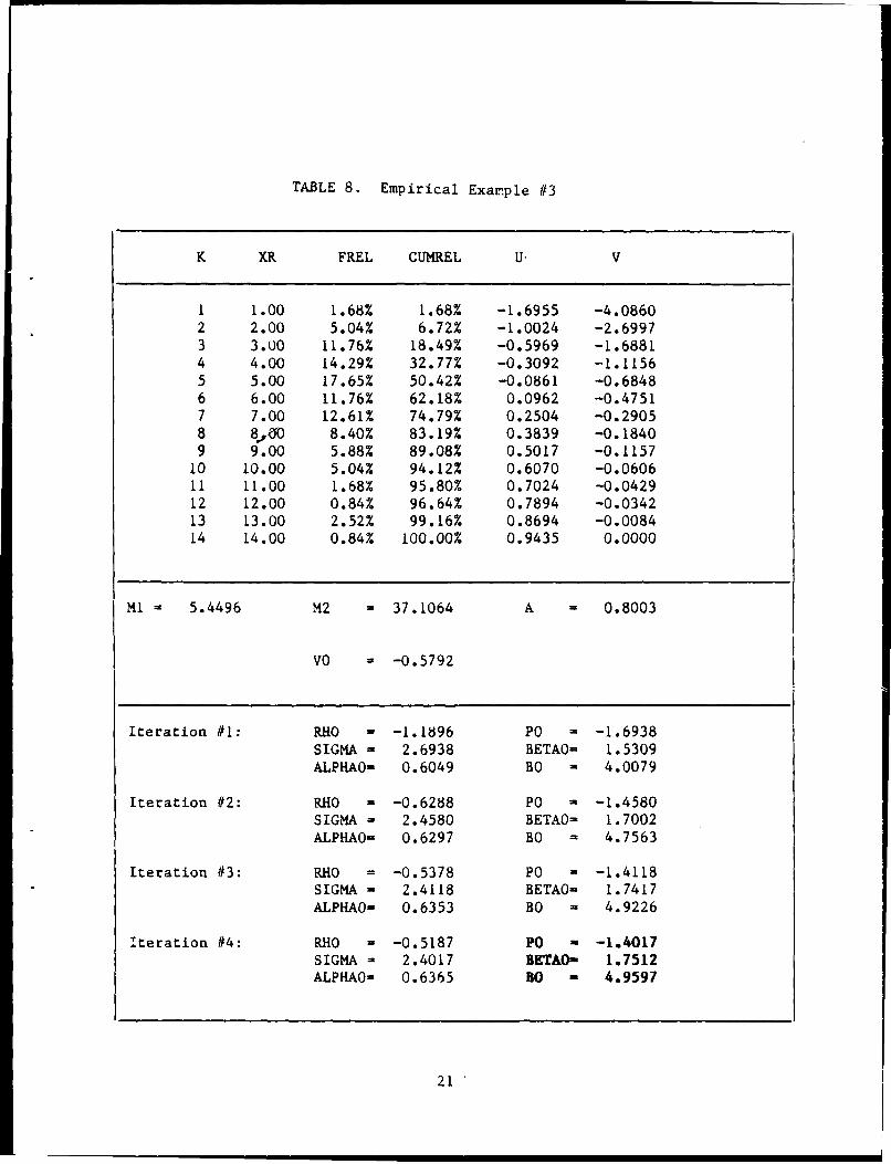
TABLE 8. Empirical Exarmple #3

K XR FREL CUMREL U- V

1 1.00 1.68% 1.68% -1.6955 -4.08602 2.00 5.04% 6.72% -1.0024 -2.69973 3.00 11.76% 18.49% -0.5969 -1.68814 4.00 14.29% 32.77% -0.3092 -1.11565 5.00 17.65% 50.42% -0.0861 -0.68486 6.00 11.76% 62.18% 0.0962 -0.47517 7.00 12.61% 74.79% 0.2504 -0.29058 8.0 8.40% 83.19% 0.3839 -0.18409 9.00 5.88% 89.08% 0.5017 -0.115710 10.00 5.04% 94.12% 0.6070 -0.060611 11.00 1.68% 95.80% 0.7024 -0.042912 12.00 0.84% 96.64% 0.7894 -0.034213 13.00 2.52% 99.16% 0.8694 -0.008414 14.00 0.84% 100.00% 0.9435 0.0000

M1 = 5.4496 M2 = 37.1064 A 0.8003

V0 = -0.5792

Iteration #1: RHO - -1.1896 PO -1.6938SIGMA = 2.6938 BETAO 1.5309ALPHAO= 0.6049 BO 2 4.0079

Iteration #2: RHO = -0.6288 Po 2 -1.4580SIGMA = 2.4580 BETAO= 1.7002ALPHAO= 0.6297 BO 4.7563

Iteration #3: RHO = -0.5378 P0 -1.4118SIGMA = 2.4118 BETAO= 1.7417ALPHAO= 0.6353 BO 2 4.9226

Iteration #4: RHO - -0.5187 Po -1.4017SIGMA = 2.4017 BETAO- 1.7512ALPHAO- 0.6365 BO - 4.9597

21

The accompanying Figures 2, 3, 4, 5, and 6 show the log cdf point plots.In Figure 4 the points P1 and P2 are not shown.

The calculations have been performed on an IBM-PC compatible microcom-puter (without math co-processor) in compiled MS Basic. For empirical samplesof frequency distributions with approximately 40 classes, actual computingtime was less than 60 sec.

The evaluation of the differences between the obtained parameter values

po, go, bo, and the original ones, p, B, b, shows that max I1po-P I. I o-IIbo-b 11 is < 6.10-2 in SYNEX #8, < 2"10-2 in SYNEX #9, < 8"I0 - 3 in SYNEX#10a, < 6.10-2 in SYNEX #10b. In SYNEX #11, max I po-p 1, Igo- It < 5.10-2,but 1.950 < bo - b < 1.951. The large error in the scale parameter demon-strates the well-known sensitivity of this parameter to small changes in theothers for J-shaped distributions. The culprit in this matter, of course, isthe error in the Initial shape parameter p. Ultimately, this error resultsfrom the fact that the class interval length in the example used is too bigfor this type of distribution.

Before closing this section, briefly return to the empirical example,EMPEX #3 considered in Section IV. The first and second moments are (from(5) and (6), respectively) Ml = Ml = 5.4496 and M2 - M2 - 37.1064 as shown inthe center block of Table 8, which also shows the numerical values ofA - M1

2/M2 and v(O) - VO. Starting with 8 - 1, after the 4th iteration step,the final parameter values bo, Po, and 80 shown in the lower right-hand cornerof Table 8 are obtained. The least squares approximations include the pointsF9 for v - 1,...,8. No goodness-of-fit test will be performed on the finalparameter values in this paper. This will be left to a separate publicationwhich will deal exclusively with empirical examples. However, it is worthmentioning that a recently performed maximum-likelihood estimation of theparameters of EMPEX #3 resulted in the final values p - - 1.466, B 1.720,and 6 = 4.795.

22

-i I

Ki

-4,

K

xx

-2

-4 H

-5 -4

II I I I

-5 - 4 - 3l - z - i. 0

U

Figure 2

o I I I

V K

-1K

I

-2

-4

-5

I, I I

-5 -4 -3 -2 -1 0

U

Figure 3

23

-4

-2

-424

-25

REFERENCES

1. Stacy, E. W.: "A Generalization of the Gamma Distribution," ANN. MATH.STAT. 33, pp. 1187-1192, 1962.

2. Stacy, E. W., and Mihram, G. A.: "Parameter Estimation for a GeneralizedGamma Distribution," TECHNOMETRICS 7, pp. 349-358, 1965.

3. Parr, Van B., and Webster, J. T.: "A Method for Discriminating BetweenFailure Density Functions Used in Reliability Predictions," TECHNOMETRICS7, pp. 1-10, 1965.

4. Harter, H. L.: "Maximum-Likelihood Estimation of the Parameters of aFour-Parameter Generalized Gamma Population from Complete and CensoredSamples," TECHNOMETRICS 9, pp. 159-165, 1967.

5. Essenwanger, 0. M.: "APPLIED STATISTICS IN ATMOSPHERIC SCIENCE,"Elsevier, Amsterdam, 1976.

6. Amoroso, L.: "Ricerche Intorno Alla Curva Deireditti," ANN. MATH. PARAAPPL., ser. 4, 2, pp. 123-157, 1924.

I,

7. Lehnigk, S. H.: "On a Class of Probability Distributions, Accepted byMATH. METH. IN THE APPL. SCI.

8. Lehnigk, S. H.: "Characteristic Functions of a Class of ProbabilityDistributions," Accepted by COMPL. VAR.

9. Lehnigk, S. H.: "Initial Condition Solutions of the Generalized FellerEquation," J. APPL. MATH. PHYS. (ZAMP) 29, pp. 273-294, 1978.

10. Lehnigk, S. H.: "Maxwell and Wien Processes as Special Cases of theGeneralized Feller Diffusion Process," J. MATH PHYS. 18, pp. 104-105,1977.

11. Harter, H. L., and Moore, A. H.: "Maximum-Likelihood Estimation of theParameters of Gamma and Weibull Populations from Complete and fromCensored Samples," TECHNOMETRICS, 7, pp. 639-643, 1965.

12. Gradshteyn, I. S., and Ryzhik, I. M.: TABLES OF INTEGRALS, SERIES, ANDPRODUCTS, 4th ed., Academic Press, New York, 1965.

13. NOAA, National Weather Service. Twice daily teletype bulletins of upper-air observations (rawin), Station KBNA (72 327).

14. Lehnigk, S. H., "Maximum-Likelihood Estimation of the Parameters of aFour-Parameter Class of Probability Distributions", Accepted by PROC.EDIN. MATH. SOC.

26

APPENDIX A

The Equation h(P,a) - 0

Return to the equation h(S,a) 0 0, 0 < A < 1, given in (10). The first

partial derivatives of h(R,a) are

ham2h [1 2(+) (i±)'(i)-A (±r () A'#

W (y) - d log r(y)/dy [12;8.360J being the psi function. If h(R*,cT*) -0for R* > 0, a* > 0, then

~h [- (1+a ) r1+a (a)(

Use of the series expansion for t(y) [12;8.362,1]

,(y) s- y 1V.o y+v 1+v

y = - '(1) being Euler's constant [12;8,367.1] results in

0

> 0, * > O, *> 0.(a* + vR*)(l+a* + v.*)(2+a* + v8*)

Consequently,

(~\ _r2(.±2a r>0;a \ - -) a.(Lh C6* >

A-1

In other words, considered as a function of a > 0 for fixed S > 0, h(Aa) hasa positive derivative at each of its zeros a. Since h(P,a) is continuous as afunction of a, it follows that, for fixed R > 0, h(S,a) - 0 can have at mostone root a > 0 and that h(R,a) increases from negative to positive valuesacross the root.

Again, if R* and a* are positive numbers such that h(8*,a*) = 0, then

T --/ (~ [2-- ,r2 +a 21+ar*)I IV-a~~

S*2

(2+a*\- (2+a,) --.

The following formula can be established,

/a*' I 2+a*\2(l+a*) W - *" (L - (2+a*) - - A* '.a sV,

Vs- - 28* <0O, R* >0O, a* >0O,(a* + vS*) (1+a* + vR*)(2+a* + v8*)

so that

= 2r2 > 0\-8/ sV >•

V-O

Therefore, considered as a function of R > 0 for fixed a > 0, h(8,a) has apositive derivative at each of its zeros. Continuity again implies that, forfixed a > 0, h(R,a) - 0 has at most one root, A > 0, and h(R,a) increasesfrom negative to positive values across the root.

To continue the investigation of the properties of the equationh(R,a) - 0 consider the ratio

C(8,a) -(A-1)

-~~ (2%+ar (a) r

which is a continuous function of A and a in the open domain 8 > 0, a > 0.Set (1+a)R-l - a, A-1 - y. Then (A-9) can be expressed as an infinite pro-duct (12;8.325.1],

A-2

C( R,) rot) r(c-) ifi( ct)~k c~))

V=o V- 0

0 < t < (i++VB)2-1 1(i+a+VB)2 (i+ao+V) 2

The infinite product converges (absolutely) for every R > 0 and a > 0 sincethe series

S(i+a+vRY-2 < 1+,q2 v-2 < 1 + j2

The inequality 0 < tv < 1 implies that 0 < C(S,a) < 1. Furthermore, becauseof convergence of the product, the series

log tv - log (I+a+vp)2

converges. Its uth partial sum is denoted byU )i

llog i++B)2 )To investigate the behavio, of the function C defined In (A-i), first

consider a > 0 fixed. Let 9 m- 1 , m being a positive integer. Then

- < log (I - <I2) < log i )< 0 (v m )

(l+C+VMl)- - (1+ 1)2

and, hence, for u > m,

qu < m log + lo --- log (2+1)2 +lg (I+v+vm-1)2)

< log (1 1 ) < 0.

A-2+( 3

A-3

Therefore,

0<Ifeu =i U /1 / / 1 \0 < lia e lir II t -, < exp log -

uV+ 1 t+ 0 /-o (2+a) 2

(2+a)2)

The right-hand side can be-made arbitrarily small if m is sufficiently large.In other words, for every fixed a > 0, the Infinite product C(R,a) will bearbitrarily small if 8 > 0 is sufficiently small, I.e., for every fixed a > 0,it diverges to zero as R + 0.

To investigate the behavior of C(B,a) for a > 0 fixed and 8 large, usethe partial products of (A-10),

P

U

1iThe denominator IT (l+a+vR)2 is a polynomial In P also of degree 2u with lead-

VMO

Ing coefficient (l+a)2 u!. Therefore, for every fixed a > 0 and for every u,

U

ppt as + W+.(l+a)2

VMO

This means that, for every fixed a > 0, the infinite product converges to1 - (I+a)- 2 , 0 < 1 - (+a) - 2 < 1, as R + + -.

From these results two preliminary conclusions are drawn:

(1) Since the function C(8,a) > 0 in (A-i) can be made arbitrarilysmall for every fixed a > 0 if P > 0 is sufficiently small, the functionh(Aa) with 0 < A < I will be negative for every fixed a > 0 if R > 0 is suf-ficiently small and

(2) If 1 - (l+a) - 2 < A, i.e., if

1

0< a < a- 1 1, (A-3)

h(A,a) < 0 for every R > 0. On the other hand, h(8,a) > 0 for every a > aAif 8 is sufficiently large.

A-4

Consequently, since h is a continuous function of R, observe that, forevery fixed a > 0A, h(A,a) - 0 has at least one positive root. Earlier itwas observed that, for every fixed a > 0, h(R,a) - 0 has at most one root.It follows that, for every fixed a > aA, h(P,a) 0 has exactly one positiveroot 8.

With the established existence of at least one point P* - (R*, a*), R* >0, a* > aA, such that h(A*,a*) = 0, discussion of the equation h(R ,a) - 0can be completed by means of the implicit function theorem. Its conditionsare satisfied in some neighborhood of P*: h(P*, *) = 0, (ha)p* > 0, (hq)p* >0, h(R,a), ha(8,a), hR(R,a) being continuously differentiable in the domain 0

< 8 < + -, qA < a < + =. Consequently, there exists a closed interval [RI,R 2 ]such that 0 < 81 < 8* < F2 and a one-valued continuous function a = 3(P) suchthat h(R,a(P)) = 0 for every RE [BI,R2]. The implicitly defined function3(g) is even continuously differentiable in (RI,A 2). Its derivative is givenby

d (R) P ( 8)) < , E ( I, 2),dR ha(Pd( 8))

i.e., '(A) is a monotonically decreasing function of R for 91 < R< A2.

The domain of existence of the implicit function 3(8) can now be extendedto all of 0 < 8 < + - by the following arguments.

Suppose U(B) could not be continued to the right of some point B > 0.Then there would exist a point F on the line - 6 B with coordinates S and a,aA < 3 < + -, such that every neighborhood of P would contain infinitely manypoints P of the graph of the function 3(B) with abscissas 8 < 8. At each ofthese points h(B,a) - 0. Then T would be a limit point of such points P.Because of continuity of h(8,a) this would implyh(8,a) - 0. But then thefunction 6(8) could be extended to the right of 8 by the original arguments.Analogous considerations apply for continuation to the left.

Since h(B,a) - 0 has exactly one root 8 > 0 for every a > aA, the rangeof a(S) is the interval (aA,+ -) and, as a consequence of monotonicity,

(8) + + - as 8 0 0, 3(8) + aA as 8 + + -.

A-5/(A-6 blank)

APPENDIX B

Approximation of v(u) by v*(u)

Return to the function v(u) defined in (8), replacing bM1-1 byr((l-p)8-1/r((2-p)8 -1 leaving, however, Mlb-1 in the argument of the $-functionunchanged for notational convenience. Then

v(u) - (l-p)u - log - (2-p) log r + (l-p) log r

+ log , 1 +-L-; - (! •u (B-1)

To approximate v(u) the function v*(u) given in(1i) was used with

v(O) - - log - - (2-p) log r + (l-p) log r

+ log , 1 +-; -

numerically to be determined by four-point Lagrange-Aitken interpolation fromgiven points of the log cdf plot.

Subtraction of v*(u) from (B-1) results in

v(u) - v*(u) - p + log 0(0) - pe8u, (B-2)

where, for notational convenience, O(u) stands for the function € as itappears In (B-I), 0(0) for its value at u - 0. Since fv(u) - v*(u)Imust besmall over a suitable u-interval and since Iv(u) - v*(u)Imust go to 0 asu+ - w, from (B-2) it can be seen that the two constants must satsi.y theequation

P - log 0(0). (B-3)

Now set (l-p)8 - = a, (Mlb-l) 8 - c, and expand D(u) into its power series[12;9.210.I],

s(u) - D(a, 1+a; - ceSu)

-1 - 2 ceRu + a _ c2 e 2 Bu - a _L c 3 e3Ru + -

i+a 1! 2+a 2! 3+a 3!

B-i

If each of the exponential functions is expanded into its power series, theseries for € can be rearranged as follows:

a 1a 1 a 1O(u) , 1 c + - - c2 - - - c3 +

l+a 1! 2+a 2! 3+a 3!

L c L (Ru) + - (u)2 + ! +L+a 12! 3!

+2a 1 c2 [L (28u) + - (28u)2 + -L (28u)3 + ""

2+a~ 3! 1L 2! 3!u)

a 13! [L (39u) +- (38u)2 + -L (3gu)3 + .""+-

The series in the first row is equal to ((O). The series in brackets In thevth following row is equal to ev u-l. Therefore,

$(u) (0) - 3Z (-1)v-1 a 1 cv (e Bu-l).S+Ea v!v-1

Denote the infinite series by A(u). Then

f(u) - (0(0)(1-A(u)0-l(0)j (B-4)

and consequently,

log O(u) - log D(O) + log(l - A(u)0-1 (o)]

Return with this expression to (B-2) and obtain

jv(u) - v*(u) I p + log[l -A(u)Di(O)] - 8uI (B5)

The identity (B-4) shows that I - A(O)0-1 (o) 1 . Furthermore, 0 < 0(0) <

O(u) < 1 for uE (- =,0), and $(u) + I as u 4 - . Therefore, 1 - A(u)o-l(0) +

D-1(0) as u + - -. Consequently,

I < 1 - A(u)$- 1 (0) < 0-I(0), uE (-®,0],

which implies

0 < log[1 - A(u)-l(0)] < - log V(0), uE (-a, 01.

B-2

From (B-5) the following estimate now results:

Iv(u) - v*(u) 1< p - log b(O) - pe ou , u <0.

If (B-3) holds, this reduces to

Iv(u) - v*(u) I< IP I eRu, u 0,

and v(O) - v*(O) - 0. Since Jv(u) - v*(u) J+ 0 as u + - , the maximum errorin the approximation occurs at some uo < 0. Therefore

Iv(u) - v*(u) l< p Je'uo uniformly in u < 0.

The error over the interval (O,u] is Immaterial since the objective isto approximate v(u) as u + -

B-3/(B-4 blank)

APPENDIX C

The Coefficient a as a Function of 9

Next the properties of the function o(P) defined in.(14) together with

(15) and (16) are investigated.

First of all, establish the fact that a(R) > OF or PE (0,+ a). For twopoints Pv - (u,,v.)(v1l,2) with uI < u2 and the point Vo - (0,v(O)'

2a)( 2 2) a 2 u .a2)D - l + u2 I +a2 -(ua+(ula2 -u2a2)

and, by induction,

D = All A2 2 - A1 2 ( M uav ua V 2

l< j<v<k

for any number c of points P. - (u., v.) with the abscissas ordered as above.Now look at the terms

upav - uai = uu(eRuv - l) - Uv(e UU-l), l<u<v<k, A > 0. (C-1)

Set 0up - x, Ru. - y, x < y, x A 0, y A 0. Then (C-I) changes into x(eY-1) -y(eX-l) and y = ax leads to the function

f(x) = xg(x), g(x) - eax - 1 - a(eX-1), g(O) - 0, (C-2)

g'(x) - aex (e-(la-)X-l)

Distinguish the three possible cases.

1. 0 < x < y - ax, 1 < a < + -, so that g'(x) > 0, x > 0. Since g(O) - 0,g(x) > 0, x > 0 and, hence f(x) > 0, x > 0. Therefore uja v - uvau > 0,0 < uu < uV.

2. x < 0 < y - ax, - - < a < 0, g'(x) < 0. This. and g(O) - 0 imply g(x)> 0, f(x) < 0, x < 0, and hence, uua. - uuau < 0, ui < 0 < uV.

3. x < y - ax < 0, 0 < a < 1, g'(x) > 0. g(O) - 0 leads to g(x) < 0,f(x) > 0, uua V - ua u > 0, 0 < uu < uV < O.

Therefore, for (C-I)

uuaV - ua. < O, uu V > 0, (C-3)<0, u11uv < 0.

C-1

Consequently, D(B) > 0, 8 (0, + -).

Next, look at DI(8).- For two points,

Dl - (ulci + u2c2)(a 21 + a22) - (alcI + a2c2)(ulal + u2a2)

- (ula2 - u2al)(cla2 - c2al)

and, by induction,

D1 - BA2 2-CA1 2- (uuav.-uvau)(cav - cjau)•

1< u<v~k

Investigate the terms

ca. - cvau - [v, - v(O)I(eRUv-l) - [vv-v(O)](e'Uu-l),

l<u<vk, 00.

Division of (C-3) by u~uv 0 0 results in

a. a.1- - > 0 in any case. (C-4)u V u11

Let r. M cuuu-1 ,rVM cVUV- , and assume 0 < r. < r.. Since r. may be

interpreted as tan 9, 6. being the angle between the horizontal positively

oriented line through P. and the line through P. and Vo - (O,v(O)), the last

assumption implies concavity of the location of the three points Pu, PV, andVo . Then, since acuK- 1 > 0, (C-4) implies

a. rV a.1S> 0 in any case.u V r. u U

Multiplication by uuuvru yields

uUr j AV - uvrva u - cta v - cvau > 0, uuuv > 0 (C-5)1< O, uUu V < 0.

On the basis of this inequality and (C-3), DI(A) > 0, R (0, + -,), providedthe points PV are concavely located. Consequently, under this concavitycondition, the coefficient a(8) of the approximating function v*(u) is a posi-tive function of 8 > 0.

The following remark is essential at this stage. In practical situations,all of the coordinates of the points Pv (v-l,...,k) of a given empirical dataset may not satisfy the inequality (C-5). Indeed, this is frequently the case.

C-2

However, violation of (C-5) will occur only for points PV with v equal orclose to 1, since the smoothing effect of the cumulative frequencies elim-inates this occurrence for large values of v. In other words, if the pointsPV are sufficiently smoothly located, D1 and, consequently, a, will still bepositive. If, however, in a practical situation, DI should turn out to bealways negative or zero, then this is a clear indication that the class (*)of distributions cannot be used for a data fit.

Turn now to the derivative of a(8) with respect to the parameter R. Itis given by

a' - D- 2 {D[BA' 2 2 - C'A1 2-CA'1 2] -Dl[AlA'22 - 2A12A'12]1 , (C-6)

k k k

A1 2 = u , A2 2 2 uvabv, C uvvc,bie'u v ...b

Starting from k = 2 one can show by induction that

BA2 2 - C'A1 2 - CA1 2 - [(uaV-uvau)(uvbvcu-uUbucV)

1< IX v k

+ u 1U v(c Va V-c va 11) (bv-b U)]

= ((cuUv-cvuu)(uuaVbp-uvaubV)

1<u<\<k)

+ 2 uuuv (cuav-cvau) (bV-bu)1 (C-7)

after addition and subtraction of uuuv (cuav-cvaU)(bv-bu), and

I IAll A2 2 - 2A1 2A1 2 - 2 F uuuv (uua-uvau) (bv-bu). (C-8)

1< u< Kk

The derivative of a(8) can now be written as

a' . D-2 1[Fueav-uvau)Z(cu-cvuu)(uuavbu-uvaujbv]

[F 2 U [ \(ija u a )] [uuv (cuav -cVau)(bV-bi)]

- 2 [Ecu~aV-uvapu CUav-cvauj)] [F1u U V(ula V-u v u) (bv-b )] 1(C9)

summations to be performed over 1 < u < v < k. For simplicity, set

Ru- M uUa V - ujau, SUV , cua v - cvau.

Then, using different subscript pairs for clearer distinction between theindividual factors, write the second and third lines in this expression for

a' as follows:

c-3

2 [FR2 11v] u cu X S KX(b X -b

-2 IF IRuV] [uuXRX (bX - ,

Those pairs of terms cancel for which the subscript pairs (u,v) and (,,X) areequal. The remaining terms are pairwise of the form

2R2 uvuKuXS X (bX-b) - 2 Rj1VSUVuuXRKX (bXI-bc), (C-10)

(u,v) A (1CX).

The error equations (13) of the least squares approximation can bewritten as

auv + pav - c v - ev (v-1, .. , k).

Division by av (A 0 since uV 0) results in

av a v av

and consequently,

( U ' C IJ C) E I . CV)a ~-i~)i(a. +v (a.~a

Multiplication by aay leads to

aRuv - + Euv (0 < U < v < k)

with Eua. - evau = Eu. Then (C-10) changes into

2R2UujcUXU (aRjcX-Ejc)(bX-bjc)-2RUV (aRjv-Eijv) UKuXRcX (bX-b<c)

= 2RUuuu(bX-bz)[EUvRK- EKXRuvj (C-11)

If, for some 8 > 0, the points Pv - (uv,vv) should all be located on the graphof the function v*(u), then ev would be zero for v-l,...,k. This would meanE1V . 0 for I < u < v < k, so that the terms in (C-11) would be zero. Hence,the derivative of a(A) would reduce from its general form (C-9) to

at = D-1 E (Cjuv-cvuj)(uuavbU - uvaubv).

1<,v<< k

C-4

In general, however, the approximation errors ev will not be zero. Then

a' - D-1 E (Cuuv-cvuu)(uuavbp - uvaubv) + D-2E (C-12)l<p<v<k

where E represents the sum of all terms (after cancellation) which are due tothe ev's not being zero.

Now establish inequalities for the factors in the sum In (C-12). Firstfor cuu - cvuu: if, as before, ru = cuul- 1, rV = cvuv

-', then r. - rV > 0if the points P, , PV, Vo satisfy the concavity condition. Multiplication of

the last Inequality by uu leads to

> 0, uuuv > 0,cjuV - cvuu < 0, uju < 0. (C-13)

Next look at

uUa b1 - u aUb = u, (eSU'-l) eRu-uv(e u1 )e uv.

Set 8up - x, Buv - y, x < y, x A O, y 0 0. Furthermore, set y - ax, andobtain the function

f(x) - -xe-(l+t)x g(x), g(x) e- ax - 1 - a(e-x-l).

With x replaced by -x, the function g(x) appearing here is the same as that In(C-2). Therefore,

u~avbu - {< , uu v > 0,

> O, uuu v < 0.

This inequality and (C-13) show that the sum in the expression (C-12) for a'Is certainly negative if the points Pv , (uV,vV) are concavely located rela-tive to each other with respect to the point Vo - (O,v(O)) (or at least thosefor sufficiently large v). Consequently, if the error term D- 2 IE I is suf-ficiently small, I.e., if the approximation of the points PV by the graph ofthe function v*(u) is sufficiently good, the derivative a' of a(P) as givenin (C-6) will still be negative.

An essential practical side result can be formulated on the basis of thelast considerations. The class of distributions (* ) may be used for an ana-lytical fit of a given empirical statistical data set if the function a(s) ismonotonically decreasing.

At the end of Appendix D this version of the applicability criterionshall be reformulated to obtain a practically more useful form.

C-5

This appendix shall be finished by an investigation of the limitingbehavior of a(R) as R + and 9 + 0. The function a(R) is defined by theexpression

BA2 2 - CA1 2 o " (C-i14)A 11A 2 2 - A

2 (-4

12

the various terms being given in (16). As 8 + + -, (since uI < u2 < ...< Uk-3 < 0 < Uk-2 < Uk-1 < Uk),

BA22 - CA12 - (B - ukck)a2 + (terms of lower order),

ALIA22 - A2 1 2 - (All - u2 )a2 + (terms of lower order).

Therefore, provided a' is negative,

k-l1: uVa,

B - ukck v1a $ a A1 l -U2 k - > 0, + + .

All-u k-1 2

v-1

As A + 0 the following is argued. Since the numerator and the denomina-tor in the expression (C-14) for a both go to zero as B + 0, the Bernoulli-deL'Hospital rule applies. It is used three times. If, in the first step,the expressions (C-7) and (C-8) are used, the following expressions arederived In the third step for the numerator and denominator, respectively,

= [uuuv(uvbv-uubu)(uvbvcu-uubucv) + (terms which go to 0)]

2 E [ 3ujuv (ubv-upbp ) (bv-bu) + uuuv(uuaV-uvau) (u 2 vbv-u 2 ub)].

Clearly, each term In the second sum approaches zero as 8 + 0. Since bV + 0as 8 + 0, the first term in the first sum approaches the positive valueuuuv(cuuv - cvuu.)(u v - uu). Consequently, a + + - as 9 + 0.

C-6

Convergence of the Iteration Process

Two functional relations have been established:

a -( A), a =( 8), 0 < 8 < + W. (D-1)

The first one is implicitly defined by the second moment equation h(q,a) = 0;the second one has been derived from a least squares fit of given log cdfpoints. The properties of U(8) and a(8) have been discussed in Appendixes Aand C, respectively. The parameter determination problem has exactly onesolution go, ao - i - po, bo, if and only if there exists exactly one valueRo > 0 such that a(%) - Fr(Ro), i.e., geometrically speaking, if, and only if,the graphs of the two functions in (D-l) have exactly one point of intersection.

Suppose now that there is exactly one Bo > 0 such that a(80 ) - a(Bo).Since U(8) is not explicitly available, use instead of (D-l) the equivalentequations

h(Ba) 0 0, a - a(8), (D-2)

and solve them iteratively.

From the least squares fit by means of v*(u) with the starting value8 - 1, exactly one number Is obtained, al - a(l) - DI(l)/D(l). Then solve theequation h(8,al) - 0, its unique solution being 81 and face the trichotomy81 - , 81 > I, 81 < I.

(a) If BI - 1, the iteration process through (D-2) produces the sequen-ces fa.1 and f8,j with av - al, 8v - 1 (v-1,2,...). Consequently, the solu-tion of the system (D-2) is 80 - 1, a0 - 1 - Po M al.

(b) If 81 > 1, sequences TavT and Jfl are obtained for which not allelements are equal. If the function a(R) is monotomically decreasing(Appendix C), i.e., if the given data are not "ill-conditioned," in the seconditeration step a number a2 = a(RI) < al = a(l), is obtained. Since h(8l,01) =

0, h(8l,a 2 ) < 0 (Appendix C). Therefore, the root R2 of h(8,a2 ) = 0 satisfiesthe inequality R2 > Rl These arguments apply in each of the subsequentiteration steps. Since it was assumed that there exists only one value Ro forwhich a( %) - Z( %), the sequence f%1 converges to 80, 8 + 80 > 1 as v + + -,and the sequence favl converges, aV 4 co -a I - Po as v + + -.

(c) If 81 < 1 analogous arguments apply to establish convergence of thesequences f8,1 and fav1 to unique limits Ro < 1, ao - I - Po, respectively.

In practice, of course, the iteration process is stopped whenever adesired accuracy has been reached, and the last 8-value is taken as Ro.

Convergence of the iteration process represents the ultimate practicaltest for the applicability of the class of distributions (*). If the itera-tion process does not converge, this is, in fact, an indication that thegiven empirical data set is ill-conditioned and that the class (*) shouldnot be applied.

D-1/(D/2 blank)

DISTRIBUTION

Copies

DirectorUS Army Research OfficeATTN: SLCRO-PH 1

SLCRO-ZC 1P. 0. Box 12211Research Triangle Park, NC 27709-2211

HeadquartersDepartment of the ArmyATTN: DAMA-ARRWashington, DC 20310-0632

OUSDREATTN: Dr. Ted BerlincourtThe PentagonWashington, DC 20310-0632

US Army Materiel System Analysis ActivityATTN: AMXSY-MPAberdeen Proving Ground, MD 21005

IIT Research InstituteATTN: GACIAC10 W. 35th StreetChicago, IL 60616

AMSMI-RD, Dr. McCorkle 1Dr. Rhoades 1

-RD-RE, Dr. R. Hartman 1Dr. J. Bennett 1.Dr. S. L. Lehnigk 10Mr. H. P. Dudel 10

-RD-CS-T, Record I-RD-CS-R, Reference 15-GC-IP, Mr. Bush 1

DIST-1/(DIST-2 blank)