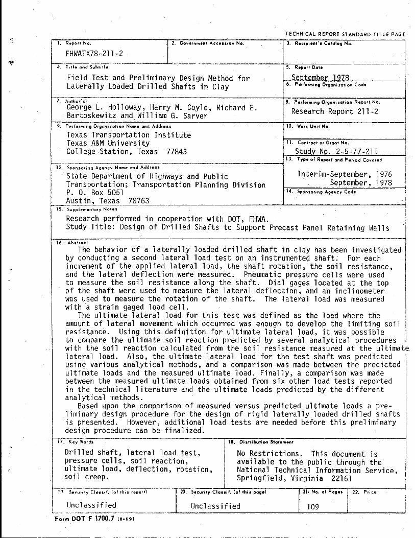
f?-; TECHNICAL REPORT STANDARD TITLE PAGE

1. Report No. 2. Government A·ceeiuion No. FHWATX78-211-2

3. Reeipi•nt' 1 Catalog No. 1 I

~4_-r::-~-:~-:-~-";-- 5-;:-t~-~. ~·~-~-Pr:-1 ,-. m_i_n_a.j...r_y_D_e_s_;9·n--M__,e--t-ho_d_f_o_r ____ -+~s=·...,s~::;o-P~~·=·~=~,_lu..0bt:•e!=r==l=Q7:':R=~-,.---~--_-_-_ .. ·_·-~1 Laterally Loaded Drilled Shafts in Clay 6. PerformingOrgonirotronCod•

7. Author's) George L. Holloway, Harry M. Coyle, Richard E. Bartoskewitz and William G. Sarver

9. P .. rforming Organization Nome and Address Texas Transportation Institute Texas A&M University College Station, Texas 77843

~----------------------------------------------~ 12. Sponsoring Agency Name and Address ·State Department of Highways and Public Transportation; Transportation Planning Division P. 0. Box 5051 ·

8. ?erformrng Orgoniution Report No. Research Report 211-2

10. Work Unit No.

II. Contract or Grant No. Studv No. 2-5-77-211

13. Type of R•part and Period Covered

Interim-September, 1976 September, 1978

14. Sponsoring Ag.enc:y Code

' I

i l i I i

Austin, Te~~~ .. --787~1._ __ .. _ --------------~---------------1! I 15. Suppl~menlory Notes

Research performed in cooperation with DOT, FHWA. Study Title: Design of Drilled Shafts to Support Precast Panel Retaining Walls

16. Abttroc:t

i I I

I

The behavior of a laterally loaded drilled shaft in clay has been investigated by conducting a second lateral load test on an instrumented shaft. For each increment of the applied lateral load, the shaft rotation, the soil resistance, 1

and the lateral deflection were measured. Pneumatic pressure cells were used to measure the soil resistance along the shaft. Dial gages located at the top of the shaft were used to measure the lateral deflection, and an inclinometer was used to measure the rotation of the shaft. The lateral load was measured with a strain gaged load cell.

The ultimate lateral load for this test was defined as the load where the amount of lateral movement which occurred was enough to develop the limiting soil resistance. Using this definition for ultimate lateral load, it was possible to compare the ultimate soil reaction predicted by several analytical procedures with the soil reaction calculated from the soil resistance measured at the ultimate lateral load. Also, the ultimate lateral load for the test shaft was predicted using various analytical methods, and a comparison was made between the predicted ultimate loads and the measured ultimate load. Finally, a comparison was made between the measured ultimate loads obtained from six other load tests reported in the technical literature and the ultimate loads predicted by the different analytical methods.

Based upon the comparison of measured versus predicted ultimate loads a pre­liminary design procedure for the design of rigid laterally loaded drilled shafts 1

is presented. However; additional load tests are needed before this preliminary design procedure can be finalized.

17. Key Wordt Drilled shaft, lateral load test, pressure cells, soil reaction, ultimate load, deflection, rotation, soil creep.

18. Distribution Stot•ment I

No Restrictions. This document is / available to the public through the j National Technical Information Service, i Springfield, Virginia 22161

I I? s~·;;;;,·t;c~ ... ,. (oj"'";h.-;~;;;,.t) ~uroty Clauil. (of thit page)

Unclassified nclassified 109 / '--------· ----------- ·------------.1..-------"--------.J

21· No. of Pages 22. Pri ee

Form DOT F 1700.7 cs-691

'0

FIELD TEST AND PRELIMINARY DESIGN METHOD FOR LATERALLY LOADED DRILLED SHAFTS. IN CLAY

by

George L. Holloway Research Assistant

Harry r~. Coyle Research Engineer

Richard E. Bartoskewitz Engineering Research Associate

and

William G. Sarver Research Associate

Research Report No. 211-2

Technical Reports Center Texas Transportation tnstJtuta

Design of Drilled Shafts to Support Precast Panel Retaining Walls Research Study Number 2-5-77-211

Sponsored by State Department of Highways and Public Transportation

in Cooperation with the U.S. Department of Transportation

Federal Highway Administration

September 1978

TEXAS TRANSPORTATION INSTITUTE Texas A&M University

College Station, Texas

Disclaimer

The contents of this report reflect the views of the authors who are responsible for the facts and accuracy of the data presented herein. The contents do not necessarily reflect the views or policies of the Federal Highway Administration. This report does not constitute a standard, specification or regulation.

There was no invention or discovery conceived or first actually reduced to practice in the course of or under this contract, including any art, method, process, machine, manufacture, design or composition of matter, or any new and useful improvement thereof, or any variety of plant which is or may be patentable under the patent laws of the United States of America or any foreign country.

ii

,,

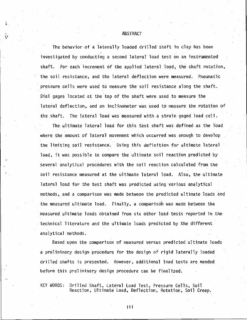
ABSTRACT

The behavior of a laterally loaded drilled shaft in clay has been

investigated by conducting a second lateral load test on an instrumented

shaft. For each increment of the applied lateral load, the shaft rotation,

the soil resistance, and the lateral deflection were measured. Pneumatic

pressure cells were used to measure the soil resistance along the shaft.

Dial gages located at the top of the shaft were used to measure the

lateral deflection, and an inclinometer was used to measure the rotation of

the shaft. The lateral load was measured with a strain gaged load cell.

The ultimate lateral load for this test shaft was defined as the load

where the amount of lateral movement which occurred was enough to develop

the limiting soil resistance·. Using this definition for ultimate lateral

load, it was possible to compare the ultimate soil reaction predicted by

several analytical procedures with the soil reaction calculated from the

soil resistance measured at the ultimate lateral load. Also, the ultimate

lateral load for the test shaft was predicted using various analytical

methods, and a comparison was made between the predicted ultimate loads and

the measured ultimate load. Finally, a comparisoh was made between the

measured ultimate loads obtained from six other load tests reported in the

technical literature and the ultimate loads predicted by the different

analytical methods.

Based upon the comparison of measured versus predicted ultimate loads

a preliminary design procedure for the design of rigid laterally loaded

drilled shafts is presented. However, additional load tests are needed

before this preliminary design procedure can be finalized.

KEY WORDS: Drilled Shaft, Lateral Load Test, Pressure Cells, Soil Reaction, Ultimate Load, Deflection, Rotation, Soil Creep.

iii

SUMMARY

This report presents the results of the second year of a four-year

study on drilled shafts (piers) that are· used to support precast panel

retaining walls. The objective of the study is to develop rational

criteria for the design of foundations for this purpose.

During the first year it was determined that many drilled shafts that

are used in this manner can be designed or analyzed as rigid structural

members. The first part of this report briefly summarizes some of the work

that has been done by others within recent years relating to the design

of rigid shafts, the prediction of lateral load capacities, and the

measurement of 1 atera·l soi 1 pressures.

A field test was conducted on a 36-in. diameter shaft embedded 15-ft

in clay. Passive lateral pressures in the longitudinal direction on the

shaft were measured with 6-in. square pressure cells. At one point on the

shaft three cells were mounted along a circumferential line to measure the

horizontal pressure distribution. Lateral displacement of the shaft was

measured at one point located about 9-in. above ground level. Rotation

of the shaft was measured by an inclinometer and also by horizontal offsets

from a plumb line to several points on the shaft. An electric strain gage

type load cell was used to measure the lateral load that was applied by

means of a hydraulic winch connected to a block and tackle.

A comparison was made between the ultimate soil reaction computed from

the test data and the values predicted by several analytical methods. A

comparison was also made between (1) the measured ultimate load and the

loads predicted by several analytical techniques, and (2) the ultimate loads

obtained from six load tests reported in the literature and the correspond­

ing loads predicted by the same analytical techniques.

iv

;r{

,>.

------------------------------ -------- ----

A preliminary design procedure for rigid laterally loaded drilled shafts

is presented. The procedure is base~d upon the comparison of the measured

versus predicted ultimate loads.

v

IMPLEMENTATION STATEMENT

A preliminary procedure has been developed for the design of laterally

loaded drilled shafts in clay to support precast panel retaining walls. The

·procedure was developed from the results of lateral load tests conducted on \

two shafts similar in size to those that wou]d be used in practice. It was

found that the ultimate lateral load in each case exceeded the load that

could be reasonably expected to occur in a normal service structure. How­

ever, in each case the shaft rotation at the ultimate load was too great to

be aesthetically acceptable. Recognizing this fact, it appears that the

design of drilled shafts for this purpose may be realistically designed on

the basis of a limiting value of rotation in conjunction with a required

lateral load capacity. Moreover, it is not known at this time what effect,

if any, the phenomenon of time-dependent soil creep will have on the

interrelationship between load and rotation. A "creep-test" is planned

for the third year of this study in order to possibly resolve this question. ,

Therefore, it is recommended that implementation of the study findings to

date should not be carried out until all test data relative to shafts in

clay are obtained and the results have been thoroughly analyzed.

vi

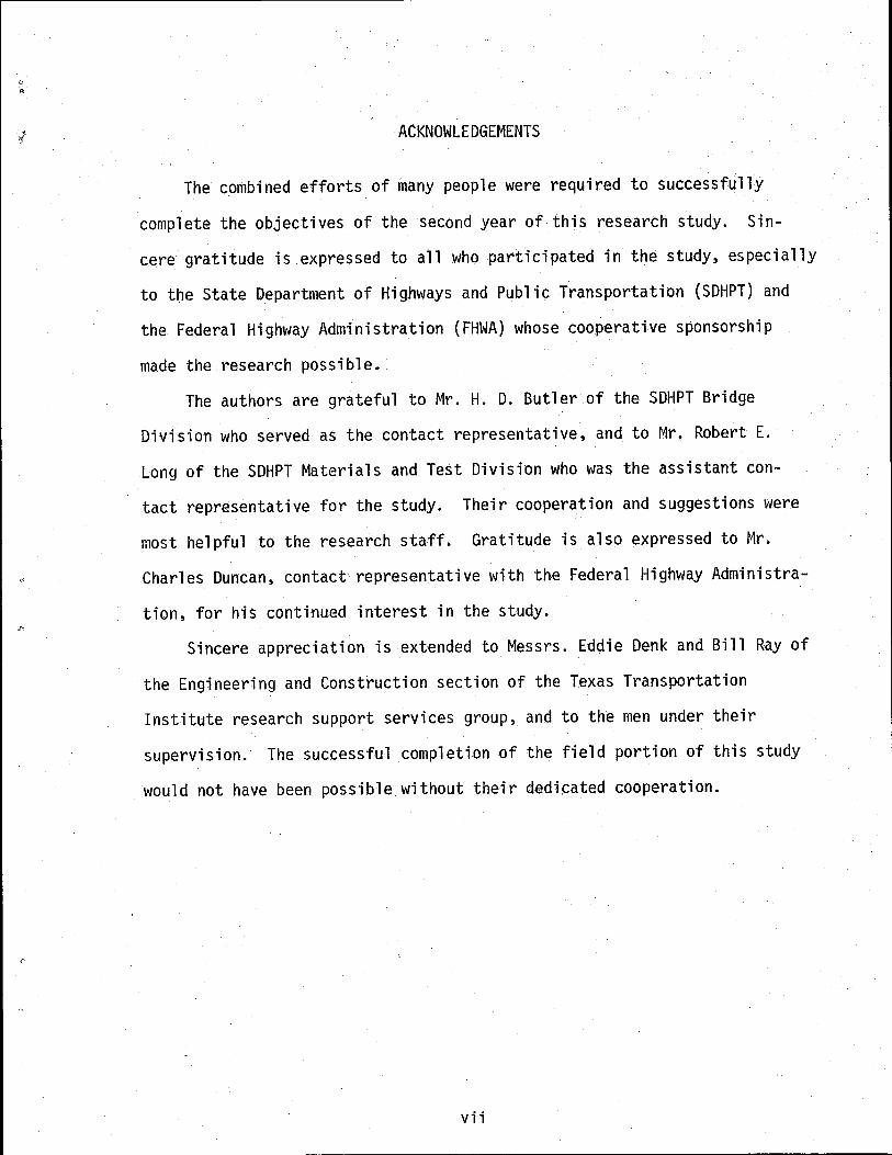
ACKNOWLEDGEMENTS

The combined efforts of many people were required to successfully

complete the objectives of the second year ofthis research study. Sin­

cere gratitude is expressed to all who participated in the study, especially

to the State Department of Highways and Public Transportation (SDHPT) and

the Federal Highway Administration (FHWA) whose cooperative sponsorship

made the research possible.

The authors are grateful to Mr. H. D. Butler of the SDHPT Bridge

Division who served as the contact representative, and to Mr. Robert E.·

Long of the SDHPT Materials and Test Division who was the assistant con-

tact representative for the study. Their cooperation and suggestions were

most helpful to the research staff. Gratitude is also expressed to Mr.

Charles Duncan, contact representative with the Federal Highway Administra-

tion, for his continued interest in the study.

Sincere appreciation is extended to Messrs. Eddie Denk and Bill Ray of

the Engineering and Construction section of the Texas Transportation

Institute research support services group, and to the men under their

supervision. The successful completion of the field portion of this study

would not have been possible without their dedicated cooperation.

vii

TABLE OF CONTENTS

INTRODUCTION . • .

Drilled Shaft Characteristics

Rigid Behavior of Laterally Loaded Cylindrical Foundations ....... .

Objectives of This Study

FIELD LOAD TEST ..

Soil Conditions

Loading System

Test Shaft . .

Instrumentation

Test Shaft Construction .

Loading Procedure

TEST RESULTS

Pressure Cell Data

Load-Deflection Characteristics

Load-Rotation Characteristics

Ultimate Soil Reaction

Ultimate Load on Rigid Shafts

PRELIMINARY DESIGN PROCEDURE . . .

Force Acting on Retaining Wall

Application Point of Resultant Force

Soil Shear Strength ....

Allowable Shaft Rotation

Soil Creep .

Drilled Shaft Design Method

viii

1

1

2

7

10

10

17

19

'21

27

29

35

35

52

52

56

61

67

67

68

68

69

71

71

Proposed Design Procedure

Example of Design Procedure .

CONCLUSIONS AND RECOMMENDATIONS

Conclusions . : .

Recommendations

APPENDIX I - REFERENCES .

APPENDIX II - NOTATION

. . . .

APPENDIX III - EXPLANATION OF SPECIAL LOADING PROGEDURES

ix

74

75

80

80

81

83

87

89

·---·------------------------------------------------------~

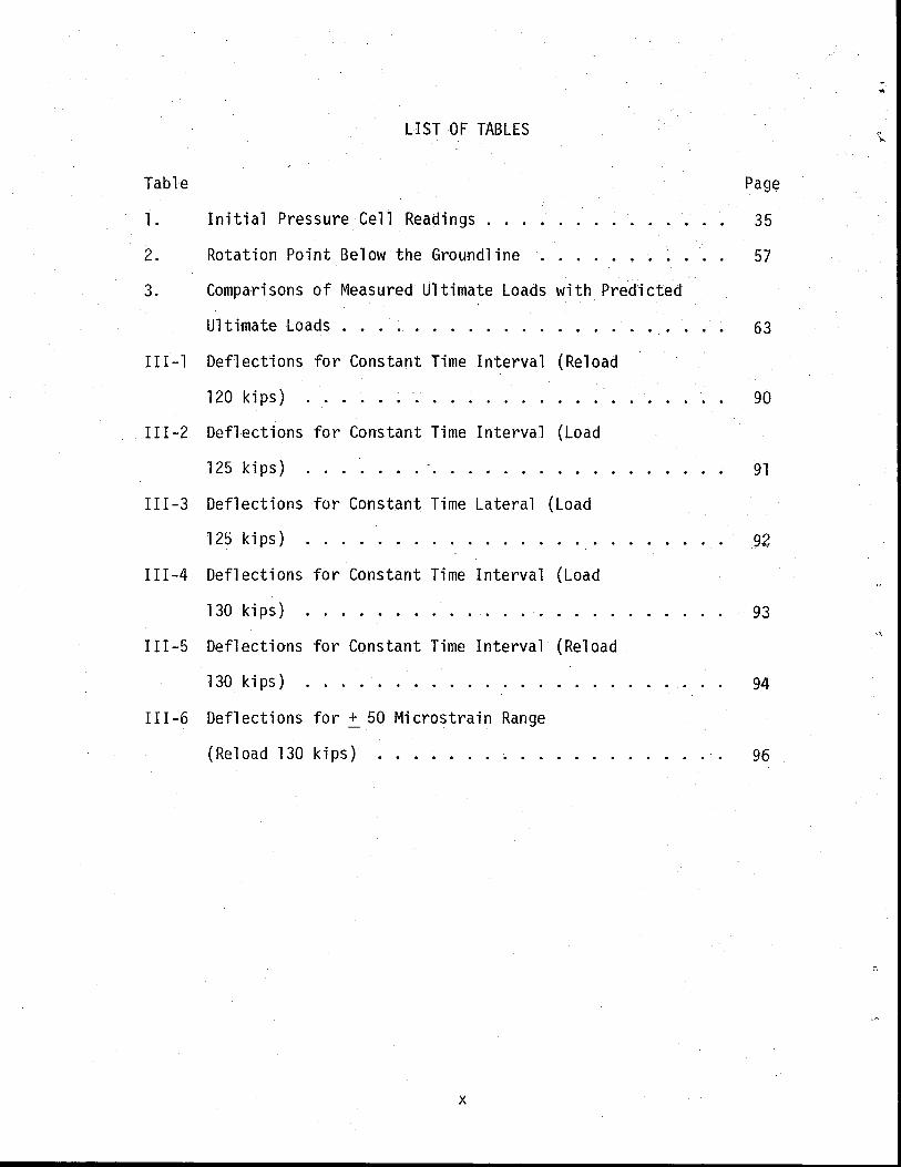
Table

l.

2.

LIST OF TABLES

Initial Pressure Cell Readings ....

Rotation Point Below the Groundline

3. Comparisons of Measured Ultimate Loads with Predicted

Ultimate Loads ........... .

III-1 Deflections for Constant Time Interval (Reload

120 kips)

II I -2 Deflections for Constant Time Interval (Load

125 kips)

III-3 Deflections for Constant Time Lateral (Load

125 kips) . . . . . . . . . . . . . . . . . . III-4 Deflections for Constant Time Interval (Load

130 kips) . . . . . . . . . . . . . . . . . III-5 Deflections for Constant Time Interval (Reload

130 kips) . . . . . . . . . . . . . . . . . . III-6 Deflections for + 50 Microstrain Range

(Reload 130 kips)

X

. . .

. . .

. . .

Page

35

57

63

90

91

92

93

94

96

~-~~~~~~~~~~~~~~~~~----

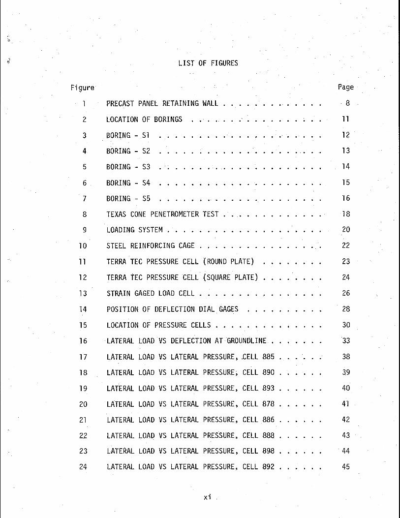
Figure

1

2

3

4

5

6

7

8

9

10

11

12

13

14

15

16

17

18

19

20

21

22

23

24

LIST OF FIGURES

PRECAST PANEL RETAINING WALL . .

LOCATION OF BORINGS

BORING - S1

BORING - S2

BORING - S3

BORING - S4

BORING - S5

TEXAS CONE PENETROMETER TEST

LOADING SYSTEM . . . . .

STEEL REINFORCING CAGE .

TERRA TEC PRESSURE CELL (ROUND PLATE)

TERRA TEC PRESSURE CELL (SQUARE PLATE) .

STRAIN GAGED LOAD CELL . . . . . . .

POSITION OF DEFLECTION DIAL GAGES

LOCATION OF PRESSURE CELLS . . . . .

LATERAL LOAD VS DEFLECTION AT GROUNDLINE

LATERAL LOAD VS LATERAL PRESSURE, £ELL 885 .

LATERAL LOAD VS LATERAL PRESSURE, CELL 890 .

LATERAL LOAD VS LATERAL PRESSURE, CELL 893 ..

LATERAL LOAD VS LATERAL PRESSURE, CELL 878 .

LATERAL LOAD VS LATERAL PRESSURE, CELL 886

LATERAL LOAD VS LATERAL PRESSURE, CELL 888 ..

LATERAL LOAD VS LATERAL PRESSURE, CELL 898

LATERAL LOAD VS LATERAL PRESSURE, CELL 892 .

xi

Page

8

11

12

13

14

15

16

18

20

22

23

24

26

28

30

33

38

39

40

41

42

43

44

45

------ -- -------------------~~~~~~~~~~~~

,_

"'

Figure Page \i

25 LATERAL LOAD VS LATERAL PRESSURE, CELL 875 . 46

26 LATERAL LOAD VS LATERAL PRESSURE, CELL 876 47

27 LATERAL PRESSURE VS DEPTH BELOW GROUNDLINE 50

28 HORIZONTAL PRESSURE VS LATERAL LOAD . . 51

29 LATERAL LOAD VS DEFLECTION AT GROUNDLINE . . . . 53

30 LATERAL DEFLECTION VS TIME . . . . 54

31 LATERAL LOAD VS ROTATION . 55

32 ULTIMATE SOIL REACTION VS DEPTH BELOW GROUNDLINE 60

33 DESIGN CHART FOR COHESIVE SOILS . . . . . . . . . . 73

xii

0

6

INTRODUCTION

Drilled. Shaft Characteristics

Drilled shafts are cylindrical foundation elements that serve

essentially the same function as piles. The only significant difference

between the two is the method of installation. Drilled shafts are

usually constructed by placing concrete in an excavated cylindrical hole,

whereas, piles are driven directly into the soil. The purpose of these

types of foundation elements is to transfer structural loads from the

surface to a depth in the soil where a more adequate bearing_strata is

found. Other terms which are used to describe the drilled shaft founda­

tion element are drilled pile, bored piles, and drilled caisson (38).

The term 11 drilled shaft 11 will be used in this study.

The manner in which a drilled shaft resists an axial load varies

according to the subsurface material and physical dimensions of the

shaft. The bearing capacity is derived from a combination of frictional

resistance and end-bearing resistance. Drilled shafts are usually

designed for end-bearing in the case where the shaft is placed through

soft or compressible deposits and supported on dense soil or rock. A

drilled shaft may also be constructed with an enlarged base in order to

provide additional end-bearing capacity (7).

Widespread use of drilled shafts began near the end of World War II.

The increased use of shafts was the result of the need by the Army for

rapid construction of light service buildings. Today, truck or crane

Numbers in parentheses refer to the references listed in Appendix I.

1

mounted drilling rigs are capable of producing holes with diameters

ranging from 12 in. to 20 ft ( 30 em to 6.1 m) and shaft depths in

excess of 200 ft (61 .Om). Battered shafts, those which are skewed from

the vertical, can also be constructed if the contractor has suitable

drilling equipment (38).

Drilled shafts have some distinct advantages over piles. The most

import~nt one is that the shaft can be drilled t6 the anticipated

bearing stratum, whereas, a pile may seek refusal in dense sand layers,

in weathered rock, or in soil with obstructions. Shafts are drilled

with virtually no displacement to the foundation soil. On the other

hand, pile driving with its associated vibrations, remolds and displaces

the adjacent soil (3). Shafts which have been underreamed provide

additional advantages over driven piles. Two advantages which are

obtained by underreaming are increased bearing capacity of the shaft

and uplift resistance.

Rigid Behavior of Laterally Loaded Cylindrical Foundations

In 1932 Sieler (32) suggested that a parabolic stress distribution

was developed along the buried length of a timber pole subjected to

lateral loads. From this early work with timber poles a design chart

was developed for calculating the required embedment depth for poles

subjected to lateral loads. This parabolic stress distribution, which

was later confirmed by Rutledge (26), Osterberg (25) and Shilts et al.

(33), satisfied statics and included the distributed effect of the soil

resistance . However, several arbitrary assumptions were made in these

studies. The most notable assumption was that the point of rotation

2

occurred at a depth of two thirds the embedment depth and that the soil

resistance was zero.

J. Brinch Hansen (12) developed a methoq for the design of rigid

foundations based on theoretical earth pressure coefficients, k and c .

kq· The coefficient, kc is determined from the product of the beari~g

capacity factor and a depth factor. The coefficient kq is the product

of the at rest earth pressure coefficient, the tange~t of the angle of

shearing resistance, and the bearing capacity factor. Hansen•s method

requires an iterative process for the summation of moments about an

assumed point of rotation. The process is quickly converging and

usually only 2 or 3 trials are necessary before a solution is achieved.

However, this method is not easily adaptable to chart solutions for

routine designs.

In two related publications, Brems (4, 5) discussed the lateral

resistance and the design of piles in cohesive soils. From studies

conducted on short rigid piles Broms determined that the ultimate

lateral soil resistance is equal to nine times the undrained cohesive

strength of the soil multiplied by the pile diameter. The soil

resistance was neglected from the ground surface to a depth of one and

a half times the pile diameter. As a result of this work, a dimension­

less design chart was developed from which deflections, embedment

depths, and maximum bending moments could be obtained.

In 1966, Ivey and Hawkins (17) proposed a method to calculate the

embedment depth of drilled shafts for the support of sign str~ctures.

The method utilizes the same parabolic soil pressure distribution as

that suggested by Sieler (32) in 1932. However, the Rankine passive

3.

earth pressure formula (35) is used to determine the maximum allowable

passive pressures. The maximum allowable passive pressure is then

reduced to an average allowable pressure by an appropriate geometric

reduction factor to fit to the parabolic soil pressure distribution.

Since Rankine's formula is based on a theoretically frictionless medium,

the presence of friction in an actual case introduces an error on the

safe side for this design procedure. In later studies directed by Ivey

(11, 15, 16, 18) a three dimensional analysis of the laterally loaded

drilled shaft problem was developed. This analysis takes into account

all shear forces acting on the shaft when determining the ultimate

resistance due to overturning loads. A series of model and full scale

tests were conducted which indicated that a modifying factor should be

introduced into the calculation of the coefficients of passive and active

earth pressure. Using the theory developed in this study, predicted

values of ultimate load are unconservative. However, the theory gives

conservative results for rotations up to 3°.

Numerous other authors (1, 7, 14, 19, 22, 35) have conducted

studies which involve the measurement of soil pressure on cylindrical

foundations by- the use of pressure cells or pressure gages. In addition

to direct measurements of soil pressure, several investigators have

reported soil reactions that were determined indirectly from instrumented

piles or drilled shafts (9, 21, 23, 30, 31, 39). The soil reactions

were determined by double-differentiation of the bending moments that

were obtained from strain gage measurements. However, before either

method of measurement was employed, the researcher had to decide whether

to use an elastic or rigid behavior analysis in determining the relative

4

flexibility of the shaft.·

The determination of whether a drilled shaft behaves either

elastically or rigidly is dependent upon the relationship between the

soil stiffness and the shaft flexural stiffness. Methods of determining I

drilled shaft behavior have been proposed by Broms (4), Vesic (37),

Matlock and Re~se (24), Davisson and Gill (8), and Lytton (20). Most of

these methods require the use of a stiffness ratio in order to determine

the relative stiffness of the shaft with respect to the soil. A compari­

son of the results obtained by the different methods shows that they

give similar results, and therefore, it makes little difference which

method is used ..

Hays et al. (13) developed two methods of solution for the rigid

pile problem. The first, being a more analytical approach, was a

discrete element solution utilizing the Winkler assumption and load

deformation curves. Using this analytical approach it was observed that

the point of rotation was not located at a constant distance below the

ground surface but shifted from somewhere below the middle of the pile

embedment depth for light loads to a depth below the three quarters

point for failure loads. The point of rotation varied at ultimate loads

for different soils and for different ratios of a·ppl ied moment to shear.

It should also be noted that this solution assumed that premature

material failure did not occur and that the lbad-deformation curves

experienced continued deflection at the maximum value of soil reaction.

The second method for the solution.of rigid pile behavior was

called the Ulti~ate Load Solution. The assumption used in this method

was th~t the soil resistance is at its maximum value along the whole

5

length of the pile, even though the maximum resistance will never be

reached around the rotation point. The solution is a quickly converging

iterative process involving the selection of trial embedment depths. It

is greatly enhanced by the development of design charts.

In 1977, Kasch (19) measured the pressure distribution in the soil

along a drilled shaft subjected to large lateral loads. The measurement

system used to measure soil pressure consisted of a series of pressure

cells placed vertically along the shaft. A load cell instrumented with

strain gages was used to measure the lateral load applied to the shaft.

The ultimate soil resistance was never developed during this test because

the test shaft failed structurally prior to soil failure. However, a

tentative design procedure was developed on the results of this test and

other existing design methods.

Although there are a number of methods which are available for

predicting lateral load behavior of drilled shafts, relatively few full­

scale field tests have been conducted which could be used to determine

the best method. Bhusham, Haley, and Fang (2) have reported on 12

drilled shaft tests. The test shafts varied in size from 2 to 4 ft (0.6

to 1.2 m) in diameter and 9 to 22 ft (2.7 to 6.7 m) in length. De­

tailed 1 aboratory investigations of the soil parameters were included for

each site. A computer program (29) entitled 11 Analysis of Laterally

· Loaded Pi 1 es by Computer," (Code name - COM622) was used to predict

lateral deflections and the results were compared with field measurement~

Using this method, the soil properties are characterized by load­

deflection curves (21, 23, 24, 31) and the flexural stiffness of the

pile is characterized in an appropriate manner to obtain compatibility

6

between the pile and soil deflection. The results of these investiga­

tions indicated that for laterally loaded drilled shafts in clay the

agreement between the measured and predicted lateral deflections was

good for deflections up to 0.5 in. (1.3 em). However the agreement

b~came progressively worse at larger deflections.

Objectives of This Study

The State Department of Highways and Public Transportation (SDHPT)

has in recent years developed a new concept in retaining wall design

and construction. The new type of retaining wall makes use of precast

panels that are placed between T-shaped pilasters. The pilasters are

spaced approximately twelve feet on centers, and are supported by

drilled shafts as shown in Fig. 1. The precast panel derives its

restraining ability from the pilasters, which are located at the edges

of the panel. The active earth pressures acting on the panel are "

transmitted to the pilasters and must be resisted by the soil in contact

with the drilled shafts. Both passive and active pressures may be

developed in the soil which is tn contact with the shaft. Since the

magnitude and distribution of these pressu~es are not well known ~nd

understood at this time, shaft designs have been necessarily conserva-

tive to ensure the long-term stability of the walls.

Wright, Coyle, Bartoskewitz, and Milberger (39) have developed

design criteria for determining the lateral earth pressures developed

in the cohesionless backfill acting on precast panel walls. As part of

this study on precast panel retaining walls, Wright, et al., instrumented

one drilled shaft with pressure cells in order to verify that this method

7

Drilled Shaft

----Panel

Pi laster

FIG. l- PRECAST PANEL RETAINING WALL

8

ti

"

could be used to measure pressure distribution on the shaft. It was

determined that the method could be used in future research studies.

A three-year research study was begun at Texas A&M University in

1977 to develop a rational design criteria for the design of drilled

shafts supporting precast panel retaining walls~ The first year of

the study was devoted to the testing of one drilled shaft and the

results have been reported by Kasch et al. (19). The test shaft for

the first year had the same dimensions as those used in the related

studies by Prescott (27) and Wright (39) on precast panel walls. As

mentioned previously, this test shaft failed structurally and some

minor problems were encountered with the loading system. Consequently,

a soil failure was not attained during the 1977 test program. However,

the use of pressure cells to measure soil pressure reaction was

successful, and their use was continued in future test programs.

During the second year of this study a test shaft was constructed

and tested in order to insure a failure in the soil. The shaft

contained enough reinforcing steel to insure that a structural failure

would not occur, and the loading system was redesigned for the

anticipated higher failure loads. Also, pressure cells were placed

on the horizontal as well as the vertical axis of the t~st shaft in

order to study pressure distributions in both directions. The test

procedure fall owed by Kasch (19) during the 1977 test was used during

the initial phase of this test program. The results of the test

program which was conducted during the second year of this research

study are reported herein.

9

FIELD LOAD TEST

The drilled shaft which was tested during the second year of this

research program was also tested in a cohesive soil. The test site was

located at the Southwest end of the Northeast runway at the Texas A&fvl

Research Annex. Not only did the test site contain a suitable cohesive

soil but also the beam-shaft reaction system was already in place from

the previous test conducted by Kasch (19) in 1977.

Soil Conditions

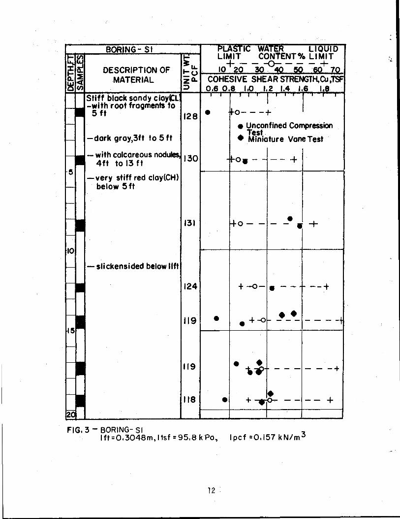
Soil conditions at the test site were investigated by making two

additional soil borings. Three soil borings had been made and one Texas

Cone Penetrometer (TCP) test had been conducted previously in the

general test area by Kasch (19). The two new soil borings were made on

January 6, 1978. These borings were designated as B-S4 and B-S5. Their

location, along with the location of the borings previously made (B-Sl,

B-S2 and B-S3) are shown in Fig. 2. Undisturbed soil samples were taken

with a 1.5 in. (3.8 em) thin-wall tube sampler. The location of the

TCP test which was conducted previously is al$0 shown in Fig. 2.

Laboratory tests were performed on the undisturbed samples in order

to determine Atterberg limits, moisture content, and total unit weight.

The undrained shear strength, C , of the cohesive samples was determined u

from unconfined compression tests. The results of laboratory tests for

each soil boring are given in Figs. 3 thru 7. These test results

indicate that the soil properties at the test site are fairly uniform.

The soil consists of stiff to very stiff clay with an average undrained

shear strength of 1.4 tsf (134 kPa). To a depth of approximately

10

1 . .,..

B-S3 •

V\

N

REACTION BEAM AND SHAFTS

I'' • .. _)

B-S2 • e TCP TEST

• B-SI

0 5 10 15 20

SCALE IN FEET

END OF RUNWAY

FIG. 2- LOCATION OF BORINGS

I ft = 0.3048 m

11

B-S4 B-S5 • •

TEST SHAFT 0

N

DESCRIPTION OF MATERIAL COHESIVE SHEAR STRENGTH.Cu,

Stiff block sandy c . -with root fragments

5 ft

-dark groy,3ft to 5 ft

128 •

-with calcareous •uu"'~ 130 4ft to 13ft

-very stiff red cloy(CH) below 5ft

-slickensided below lift

131

• Unconfined Compression Test

• Miniature Vane Test

• - -- +

o--- • +

124 + -o- • - - -- +

119 • .+ ••

119 •• ----- -+

118 • ---- +

FIG, 3 - BORING- 51 lft=0,3048m,ltsf =95.8 k Po, lpcf =0,157 kN/m3

12 .

" "

5 ft root frooments to 126 0 •

nroy, 3ft to 7ft • Unconfined Compression .. Test

• Min ioture Vane Test -becomes cloy(CH)below

4ft 3 -with colc;oreo_ys

1.

1

ond pockets, 5ft

-red below 7ft 131

-slickensided below lOft 128

8

0

• 2.03 ......

. 121 • • 0 • 0 ..

123

119

1.53+ .__.... ?,• • •

t-----+---,---1---- I. 53+ ----f • •

FIG. 4 ~ BORING-52 lft=0.3048m,ltsf=95.8 kPo, lpcf =0.157 kN/m3

13 .

122

131

-light brown, 5ft to lOft -with calcoreo~s 133

and pockets,5ft to

-becomes cloy(CH)M~nw• 5 ft

-red and slickensided below lOft

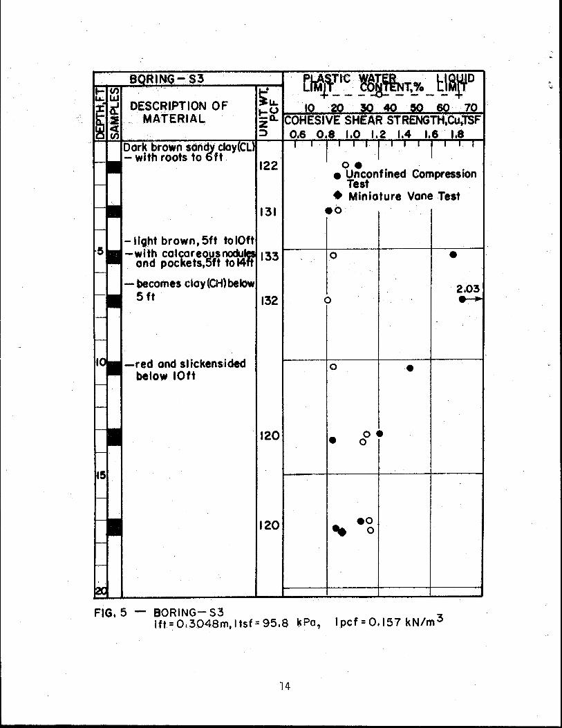
FlG. 5 - BORING- 53

132

120

120

1ft= 0.3048m, I tsf = 95.8 !)(Po,

14

oe e Unconfined Compression

Test • Miniature Vane Test

eo

0

0

• 0 0

eo .. 0

•

lpcf=O.I57 kN/m3

e

2.03

BORING- 54

DESCRIPTION OF MATERIAL

- very stiff block sandy cloy

-gray- 3ft to 8ft

PLASTIC WATER LIQUID LIMIT CONTENT,0/o LIMIT +----0----+

10 20 40 50 60 70 COHESIVE SHEAR STRENGTH,Cu, TSF

UNCONFINED COMPRESSION TEST

0.6 0.8 1.0 1.6

1---.....::;;.-+- - - - + ---1

-becomes cloy (CH) below 4ft 127

-with co lcoreous nodules and pockets, 5 ft to 13ft

red and slickensided below 10ft

FIG. 6- BORING- 54

L 126 1----+0 0 +- - ·- +

0 0 - - + ---+----1·

I ft = 0.3048 m, I tsf = 95.8 kPo, I pcf =0.157 k Nfm3

15

BORING-55

DESCRIPTION OF MATERIAL

- stiff black sandy cloy(CL) root fragments to 4ft

-with calcareous nodules · 4ft to 13 ft

- very stiff red cloy (CH)

, - slickensided be.low 9ft

FIG. 7 - BORING- S5

1-~LL. f-.:'U -l:l. z :::>

PLASTIC WATER LIQUI 0 LIMIT CONTENT,% LIMIT + - - -....... o-. - - - +

10 60 70 COHESIVE SHEAR STRENGTH,Cu,TSF

UNCONFINED COMPRESSION TEST

127 t----+- 0 •--+- ·-~----t

0 0 127 1-----+-. ---+-----t-.

00 1.95.

125 J----+----+--

lft=0.3048 m, ltsf= 95.8 kPa, I pcf =0.157 k N Jm3

16

5 ft (1.5 m), the clay was classified as a CL according to the Unified

Soil Classification System. The clay immediately below the 5-ft (1.5 m)

depth was classified as a CH. A slick€nsided structure·was noted in the

clay at depths below 10ft (3.0 m). The average undrained cohesive

shear strength determined by the buderstadt (10) methods which involves

the use of theN-value (blow count) from the TCP test, was 1.15 tsf

(110.2 kPa). The TCP shear strength data are given in Fig. 8. The

average of 1.15 tsf (110.2 kPa) compares well with the average of

1.4 tsf (134 kPa) obtained from the unconfined compression test~

Upon completion of the boring B-S3 in July 1977, ~n open end stand

pipe was installed at the site in order to make ground water observa­

tions. A perforated PVC pipe, covered with screen wire was placed in

the bore hole and surrounded with clean gravel. The water level read­

ings recorded throughout the year indicated that the level was steady

at a depth of 18.8 ft (5.73 m).

Loading System

As stated previously, the test site is the same as the one used by

Kasch (19) for the twenty foot deep drilled shaft test conducted during

the first year of this study. Therefore, only a few modifications

needed to be made in the existing loading system to accommodate the new

test shaft.

The loading mechanism was moved to the opposite end of the reaction

slab, so that the load could be applied in the opposite direction from

the earlier test. The reason for repositioning was to insure that the

new test shaft would not be tested in disturbed soil.

17

~ UNDRAINED COHESIVE SHEAR STRENGTH.Cu, TSF ...

•

14 0.94 •

18 1.21 •

• 18 1.21

17 1.14 •

16 1.07 •

1.01

1.07

FIG.8 -TEXAS CONE PENETROMETER TEST lft=0.3048m,ltsf=95.8k Po, lpcf=O,I57kN/m3

18

The pulley blocks used for this second test consisted of two six

sheave, 100-ton (890 kN) capacity blocks with an equalizer attached.

This gave the loading system a 14:1 mechanical advantage. The use of

the equalizer on the blocks not only added two additional strands of

wire cable but also decreased the tension in the indivi~ual strands.

Another factor which influenced the decision to use a greater number of

strands was the capacity of the hydraulic winch. It was observed from

the first test that it was very near its maximum capacity when the

structural failure occurred. The complete loading system is shown in

Fig. 9.

Test Shaft

The test shaft was located approximately 20ft (6.1 m) center to

center on line from the reaction slab. The shaft was nominally 3 ft

(0.9 m) in diameter by 15 ft (4.6 m) in depth. Due to some wobble

of the auger bit during dri 11 ing, the first few feet of the shaft was

slightly larger than 36-in. (91 em) in diameter. The final depth of

drilling was recorded as 15.1 ft (4.61 m).

The amount of steel was increased substantially for this test in

order to insure that a structural failure would not occur. The

reinforcing cage consisted of 12 No. ll bars (grade 60) with a No. 3

spiral at a 2-in. (5 em) pitch for the first 6ft (1.8 m), and a

6-in. (15 em) pitch for the remaining depth. Inside the 32-in.

(81 em) diameter cage, twelve additional bars were spaced equally at a

24-in. (61 em) diameter. Each bar was 15.5 ft (4.72 m) long and 1.5 in.

(3.8 em) in diameter, and the top 6-in. (15 em) was threaded with a

19

N 0

T 4FT

j_

~ '-""'

~ I --......._ -.. !""'--.,.,.. / '\.

-.. / '\. i< - /

"" :..--

,..,. :::~

~ ; ~ ~~ :>> <) c:::~ <: :::> .:::::

t::=-< ::::> ~ t::::o < -..:> fc:::: ~> <

.,.,.. fc::::

< :::::>

~ t:::>

:::::> ::::::::-< 1.::::: :::::> ::::::::-< ::;:;. fc:::: ::::::::-< ~> f::: ;::> < ~:> f::: ::::::=-< r-· fc:::: ~o--> :::::p. f< ~:> 1.::::: :::p. 1<: ~~ 1<:

f::: t:::P. 1-p. f::: -1.::::: 1---"' 1<:

,....... ~p

f<: 1<: t:::P.

-~p. ..- (::::P. 1..-- 20 FT -------....,..14---...4 I......:

FIG. 9- LOADING SYSTEM I ft = 0.3048 m

12WF 120~ I

LOAD CELL) I

"""---1L.::-4_:__-II •

I 2.6FT

·I~

15FT

~3FT1

~20FT ~I

ll;) ! (

1.375 in. (3.492cm) universal thread. The reinforcing steel configura­

tion is shown in Fig. 10.

A 12 WF 120 steel column was bolted to the test shaft using the

threaded reinforcing bars. The steel column served the purpose of not

only allowing the lateral load to be applied at a reasonable distance

above the ground surface but it also served as a reference point for

making inclination measurement during the testing program.

Instrumentation

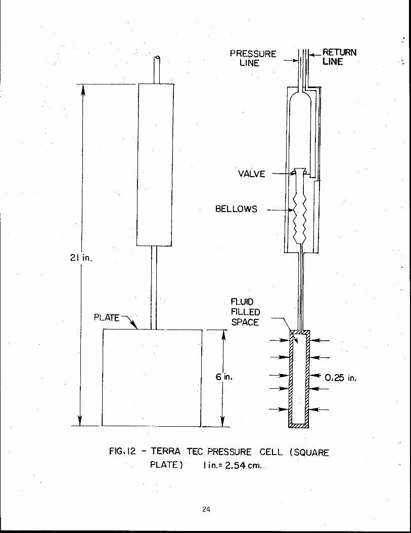
Pressure Cells. - The test shaft was instrumented with Terra Tee

pressure cells. These cells were used successfully during the related

studies by Wright et al. (39) and Kasch (19). Three cells were

retrieved from the test shaft used in 1977 and were reused along with

seven new cells for this test. The newer cells have a different shape

than the older cells but the basic principal of operation is the same.

The older cells (round plate) and the newer cells (square plate) are

shown in Figs. 11 and 12 respectively. Before the cells were installed

in the testshaft, they were individually-calibrated in a pressure

chamber. The zero reading of each cell was determined and no malfunc­

tions were observed in any of the cells. The installation of the

pressure cells was greatly enhanced by the use of a template. This

template was lightly tapped against the soil to produce a flat surface

for the face of the cell to rest against. Meta 1 pins were then driven

into the soil to hold the cells in place.

Load Cell. -The load applied to the test shaft was measured by a

200-kip (890 kN) capacity strain gaged load cell. This load cell, which

21

-r-- ,-,... ~

6 f ft (@ 2 in TCA-N0.3

RAL PI SPI

12 NO. II Gr60 BARS

12- I lf2 in { 14 5} G r 60 BARS

-~ ~

!---i< ~ - "- - > -I--

c t 1-" ~ t-- 1-- -p..

5ft -f-- I"""'

< ~ ......... io-.. 1-- 1--

I--> f--

ic: F::: I-' '- 1-- 1--> --1--~ foe ~ t-- 1-- --> ~ --

foe F: --1-- --> --~ - f--

i< - 1-- 1-- > f-- I--

foe F: --r- I-1- > - i- I-< ~ -r- ..._

I-1- !'-......

~36in -J

-r-

9 p 5

~

ft@ 6 in ITCH NO.3 PIRAL

FIG. 10- STEEL REINFORCING CAGE I ft = 0.3048 m

22

15 ft LONG, TOP 6 in THREADED 3/8 in·l2 THREADS

24in.

FRONT VIEW

PRESSURE LINE

SIDE VIEW

VALVE

FLUID FILLED SPACE

PRESSURE lN MATERIAL ·

9 in. 025. . ln.

FIG. II-TERRA TEC PRESSURE CELL (ROUND PLATE} I in. = 2.54 em

23

21 in.

PL

rc

'

ATE~

PRESSURE LINE

VALVE

BEL LOWS

'

6 in

~~

FLUID FILLED SPACE

RETURN LINE

0.25 in.

FJG, 12 - TERRA TEC PRESSURE CELL (SQUARE PLATE) I in.= 2.54 em.

24

was the same one used by Kasch in 1977 (19), had to be modified becausf~

an elongation had occurred in the connecting pin holes. This elongation

occurred from a chain reaction of events after the connecting plate

material yielded. This yielding introduced a moment fnto the connecting

pins and caused a failure of the pins. After the pins failed, the yoke

expanded due to movement of the pins and this caused the connecting pin

holes to elongate. The modifications were accomplished by increasing

the diameter of the connecting pin holes from 1.00 in. (2.54 em) to 1.50 in.

(3.81 em) diameter. The connecting pins were threaded on the outside of

the-load cell with a 1.25-in. (3.18 em) coarse thread before being heat

treated. These measures were taken so that the pins would be in double

shear and would not allow moment to be transferred into them. A

schematic of the load cell is shown in Fig. 13.

The load was measured with a Budd P350 indicator in units of micro-

strain and converted to kips by a predetermined calibration constant.

The accuracy of the load cell and Budd indicator was approximately.:!=_ .04

kips (0. 18 kN).

Inclinometer. - The rotation of the shaft was determined using a

Hilger & Watts TB108-l inclinometer. The rotation was measured in

degrees to an accuracy of approximately plus or minus one minute.

Rotational measurements were made by placing the inclinometer at five

predetermined locations on the steel column. A back-up system was also

devised for the determination of the shaft rotation. A horizontal

measurement from a vertical reference line to the five points on the

steel column allowed the determination of the relative movement of the

points. A reference line was e~tablished by a plumb-bob suspended from

25

SECTION A-A

A'---~--+---

Fl G, 13 - STRAIN GAGED LOAD CELL

26

CONNECTING PLATE ,_______, CGJNECTING PIN

~-YOKE

CO\JNECTING NUT

LOCATION OF STRAIN GAGES

SIDE VIEW

--+-+-'A CONNECTING

.._____ PLATE

a frame welded to the top of the column. Initial measurements were made

before the lateral load was applied. The initial measurements were

substracted from subsequent measurements in order to obtain the movement

relative to the initial position of the plumb line.

Dial Gages. - The deflection of the shaft at the ground line was

measured using two 0.001 in. (0.03 mm) dial gages. The gages were

attached to threadable rods which were mounted on a steel beam that was

located 18 in. (46 em) behind the shaft. The beam was supported by

two footings which were placed approximately 7.5 ft (2.29 m) on each

side of the shaft. An overhead view"showing the position of the dial

gages is given in Fig. 14.

Test Shaft Constructipn

The construction of the test shaft was accomplished in March 1978.

Experience gained during construction of the test shaft in 1977 indicated

that shoring would be needed after the soil excavation. Shoring was

accomplished by tying 2 in. x 4 in. (5 em x 10 em) boards 15ft (4.6 m)

long to the outside of the reinforcing cage. A metal flashing was also

attached to the cag~ on the front and back ~n line with the applied load.

Holes had been cut in the flashing to indicate the location of the

pressure cells with respect to depth. This served the purpose of

reducing working- time during location and installation of the pressure

cells. The reinforcing cage, with the shoring and metal flashing

attached, was lowered into the excavation in the proper position. After

the cage was in position the tie wires were cut, and the boards and metal

flashing were forced against the side of the excavation using wooden

27

-----------------------------

N CXl

TOP VIEW

SUPPORT BEAM

FOOTING 1.5 FT DIAMETER

APPLIED LOAD

0

, CONCRETE SHAFT '..- DIAMETER= 36 IN

~DIAL GAGES

SUPPORT BEAM

1.. I (5,0FT--c 7.5 FT

FIG. 14- POSITION· OF DEFLECTION DLAL GAGE I ft = 0.3048 m

:I

:;_ ~ ~

blocks.

The location of the pressure cells on the test shaft is shown in

Fig. 15. Eight of the cells were installed along a vertical line in the

plane of the applied load, and the remaining two cells were installed in

the horizontal plane perpendicular to the vertical plane at a depth of

4.5 ft (1.37 m). Seven of the pressure cells were placed on the front of

the shaft facing the loading system and the remaining three cells were

placed on the back of the shaft. The cells were placed in the soil

along the side of the excavation and held in place by steel pins. Care

was taken to insure that each cell was implanted firmly in the soil.

The shoring was removed and the concrete was placed in six consecutive

layers. A vibrator was used to insure consolidation of each layer. Con­

crete cylinders taken during the construction of the test shaft had an

average 28-day strength of 4130 psi (28,480 kPa). The' shaft was

allowed to cure for 62 days before the first load was applied on May 24,

1978. Cylinders tested at this time had an average compressive strength

of4570psi (31,510 kPa) .

. Loading Procedure

The loading procedure for this test shaft was a combination of two

previous procedures reported by Wright et al. (39) and Kasch (19).

Wright et al. developed a method for calculating the maximum resultant

force of the backfill acting on a retaining wall. Kasch (19) simulated,

on the shaft tested in 1977, the backfilling process of the retaining

wa 11 and the overburden pressure imposed by the backfi 11 on the retain­

ing wall, during a six-day period. At the conclusion of the six-day

29

I I I I

15ft.

~3ft.~

LATERAL LOAD r

2.6ft.

CELL NO.

X= 2.0 ft.

X= 4.5 ft.

X= 6.0 ft.

X= 7.5 ft.

X =9.0 ft,

X= 11.0 ft.

X= 12.5 ft.

X= 14.0ff.

885

876, 890,875

893

878

886

888

898

892

SECTION A-A

A

D

0

0

D

.-- .... I I !. __ _.

r--, I I

L--'

r--, I I L __ I

FIG, 15 -LOCATION OF PRESSURE CELLS X= DEPTH

BELOW GROUND LINE; I ft.= 0. 3048m

30

" v

period, a 13-day period of 11 Constant load'' was maintained. This was

done in order to determine if any creep was ·occurring in the soil along

the front of the shaft. However, neither of these two simulations pro­

duced any significant results at this relatively low load level. The

simulation of the overburden pressure did not cause any noticeable

changes in the pressure cell readings and consequently was not used in

this latest test.

The lateral loading procedure began with a 5-kip (22 kN)

incremental load being applied four times each day for the first two

days. The loads were applied, readings were made on the pressure cells,

and inclinations were measured after each load movement stabilized. The

stabilization time was usually 10 to 15 minates after the 1oad was

applied. During the first two days of the loading procedure an attempt

was made to simulate the loading schedule that occurred on the shaft

reported by Wright et al. (39). The total lateral load was equal to

40 kips (178 kN) at the end of the first two days of loading. No

large movements or unusual rotations were observed. At this point, it

was decided to continue this 5-kip (22 kN) incremental loading

procedure.

At the 60-kip (267 kN) level the load-deflection curve was

deviating significantly from the one presented by Kasch (19) as shown

in Fig. 16. Therefore, the decision was made to slow the loading

procedure to 5 kips (22 kN) only twice a day. A large crack was

beginning to form along the back of the drilled shaft at this time in

the loading program and deflections at the top of the shaft at ground

level were beginning to take longer to stabilize. It was also noted that

31

some creep was beginning to occur during the 24-hour period between load­

ings. After four days of twice a day loading the load.;...deflection curve

was continuing, to deviate from Kasch's (19) curve as shown in Fig. 16

for the loo~ktp {445 kN) level.

Hre new curve a:lmost paralleled the earlier curve but at a

much lower l~ad. After projecting the trend of the new data on the

load-deflection graph, the decision was made to slow the loading pro­

cedure down even further. There were two reasons for this. First, it

was necessary to establish theultimate resistance of the soil, and

secondly, small deflections were occurring for hours after the load was·

applied. By the time the new load increment was to be applied the

following day, the previous load had usually fallen off approximately

15 kips ( 67 kN). Therefore, instead of beginning with this 1 ower

load and adding a new load of 5-kips (22 kN), the load was first

brought back to where it had been the previous day. Pressure readings

were made and then an additional load of 5-kips (22 kN) was added so

as to limit the amount of differential load being applied to the test

shaft at any given time. Bringing the load back to the previous load

each day before the new load was added was considered necessary so that

the ultimate resistance of the soil could be established.

Beginning at the 115-kip (512 kN) load level, large deflections

were observed when the load was brought to the previous level. In

addition, small deflections were continuing as the load was returned to

its previous value in order to establish a stabilization point. Two

different methods were used to determine if and when the movement

ceased at a given constant load. These methods are outlined in detail

32

w w

£ ll"' 0-:;

180

I I I I I I __L-6 160

140

(/')

Cl. 120 ::t:: .. 0 ~ 100 _J

_J 80 .~

~~I ,/_/'0 1/ /. I 'I I I 6-A 1977 Test _J - - o-o 1978 Test

0------~~----~----~~----~----~~----~~--~ 0.5. 1.0 1.5 2.0 2.5 3.0 3.5 DEFLECTION AT GROUNDLINE, in.

FIG. 16- LATERAL LOAD VS DEFLECTION AT GROUNDLINE I kip = 4.45 kN; I in. = 2.54 em

and the corresponding data are presented in Appendix III.

It was believed that from the 115-kip (512 kN) load level to the

end of the loading program the deflections were both a function of the

time the load was held and the amount of load on the shaft. This value

of 115-kips (512 kN) will be considered the ultimate load for this test

and will be used for comparison with other methods ( 4, 12, 13, 16, 17) of

determining ultimate soil reaction. However, it was decided to continue

loading the shaft so additional pressure measurement could be taken at

higher loads. Loading was continued up to 150-kips (668 kN) to

determine if the shape of the pressure distribution along the shaft

might change with respect to depth below the surface.

34

TEST RESULTS

The data obtained from the full-scale lateral load test conducted

during May and June 1978 are given in this section. Pressure cell data

are presented and analyzed along with the test shaft deflection and

rotation results. A comparison of the ultimate ~oil reaction predicted

by different theories with the actual behavior of this test shaft is

discussed. Also, a comparison is made between methods which predict the

ultimate load on rigid shafts.

Pressure Cell Data

Initial Pressures. - Three sets of pressure cell readings were made

before the first lateral load was applied on May 25, 1978. These read-

ings are shown in Table 1.

TABLE 1. -Initial Pressure Cell Readings

Zero Reading In Shaft Before In Shaft Before Cell From Lab Concrete Lateral Load

March 1978 March 23, 1978 May 24, 1978 psi psi psi

875 7.5 7.5 8.1 876 15.0 16.0 18.2

878 8.0 8.5 6.1

885 3.5 3.0 2.4 886 4.0 5.0 1.3 888 3.25 3.9 3.0 890 3.0 3.5 1.05 892 3.0 4.5 4.5. 893 1.0 1.0 3.6 898 3.0 4.0 8.6

NOTE: 1 psi = 6.895 kPa

35

The readings presented are: (1) the zero readings from the labora­

tory calibration; (2) the initial readings taken after the cells were

installed in the shaft, but before the concrete was placed; and (3) the

readings taken 30 days after the concrete was placed and before the first

lateral load was applied. These pressure measurements (before concrete

and before load) were used for determining the total pressure change of

the shaft and the amount of pressure change due to the lateral load

applied. As shown in Table 1, the initial zero readings taken in the

shaft differed from the zero readings obtained from the laboratory

calibration. The pressures in the shaft ranged from 0.5 psi to 1.5 psi

(3.4 to 10.3 kPa) higher than the laboratory calibrations except for

one pressure cell. This cell (No. 885) was located two feet below the

ground surface and recorded a pressure of 0.5 psi (3.4 kPa) lower

than the laboratory calibrations. The reason for the pressure being

lower is not known. However, this general trend of an increased pressure

was expected because of the way the pressure cells were attached to the

wall of the shaft during installation.

The cells were read again 30 days after the concrete was placed.

There is not a consis.tent trend for this set of readings .. Four of the

pressure cells recorded pressures ranging from 0.6 to 4.6 psi (4.1 to

31.7 kPa) higher than the in shaft before concrete measurements and

the remaining six cells recorded pressures ranging from 0.6 to 3.7 psi

(4.1 to 25.5 kPa) lower than the in.shaft before concrete measure­

ments. The placement of the concrete or the concrete shrinkage during

the 30-day curing time could have caused these fluctuations in the

initial pressure cell readings.

36

Pressures During Lateral Loading. - The lateral soil pressures that

resulted from the lateral loading of the drilled shaft were obtained by

subtracting the initial cell readings from the cell readings for a

particular lateral load. The initial cell readings were obtained on

May 24, 1978, just prior to the application of the first lateral load.

The lateral soil pressures obtained for each cell throughout the test

are plotted on Figs. 17 thru 26. Most of the curves show a gradual

increase in pressure as the lateral load was increased. However, cells

878 and 888 (see Fig. 15) showed an erratic pressure behavior. This

behavior could possibly be explained by the point of rotation shifting

downward during the increase of the lateral loading which could cause

lower pressures than previously recorded. The two bottom cells (898 and

892) indicated negative pressures at the beginning of the test and did

not begin to show positive pressures until the 80-kip (356 kN) and 40- .

kip (178 kN) load levels, respectively. A possible reason for the

occurrence of negative pressures could be that some of the clay may have

fallen out from behind the cells during installation and created an

insufficient bearing area for the cell plate. The reason these cells

did not begin to indicate any significant pressure increase as soon as

the other cells did, may be because of their location on the shaft.

Since these cells were the two bottom cells, it would probably take

longer for the load to be felt at these depths. It is also important to

note, that cell 898 did not indicate a positive pressure as soon as cell

892. This behavior would be expected, because cell 898 was 1.5 ft

(.46 m) above cell 892 (see Fig. 15) and the distance to the point of

rotation was greater for cell 892. Thus, cell 892 experienced positive

37

20

p 0------~------~----~------~------~~ 20 40 so so roo 108

LATERAL PRESSURE, PSI

FIG. 17- LATERAL LOAD VS LATERAL PRESSURE, CELL885 I kip = 4.45 kN; I psi = 6.89 kPo

38

0

v

140.-----~-------r------~------r-----~----n

CELL 890

100~----~------~------4----

U>SQ a.. ~ .. Q <( 0 ...J

60 0

...J 0

<t 0 0:: w !:i

5 .-·' ·--· 40

201----

10 20 30 40 50 57 LATERAL PRESSURE, PSI

FIG. 18- LATERAL LOAD VS LATERAL PRESSURE, CELL 890 I kip =4.45 kN; I psi = 6.89 kPa

39

140~-r------~------r-----~-------r------·U

CELL 893 l2011---+---~----t-----t-----'--

~100 ~ .. Cl <( 0 ...J 80 ...J <( 0:: w .._ <(

...J 60

40

• 0

0

I • _,

!J !.i

0 10 20 30 40 50 LATERAL PRESSURE, PSI

FIG. 19- LATERAL LOAD VS LATERAL PRESSURE , CELL 893 I kip = 4.45 kN; I psi = 6.89 kPa

40

0

"

140~----~------~------~------------~

CELL 878

~ 100 ~ .. 0 <( 0 ....1

....1 <( 0:: w t:r ....1

80

0

0 0

60 • 0

l..i

·-.. f.!

40

20r---

3 6 9 12 15 LATERAL PRESSURE, PSI

FIG. 20- LATERAL LOAD VS LATERAL PRESSURE, CELL 878 l kip = 4.45 kN; I psi = 6.89 kPo

41

14Qr------,..-----,----..-or------rl------.

(f.) 100 a.. ~ .. 0 <{ 0 _J 80 _J

<t 0:: w ~ _J 60

40

CELL 886

0

0

• . ~ ~· .~ _, !..1

10 20 30 40 50 LATERAL PRESSURE, PSI

FIG. 21- LATERAL LOAD VS LATERAL PRESSURE, CELL 886 I kip = 4.45 kN; I psi = 6.89 kPo

42

: ·...;

" 140

120

(/) 100 0.. ~ .. 0 <( 0 80 ..J

..J <( 0::: w ~ ..J 60

40

20

0

I~

CELL 888

/v 7 ,..1

] 0

~ 0 (

0 0

}1 0

• ,. -· ,. _, '---

p

2 4 6 8 10

LATERAL PRESSURE, PSI

FIG. ·22- LATERAL LOAD VS LATERAL PRESSURE, CELL 888 I kip = 4.45 kN; I psi = 6.89 kPa

43

140

CELL 898 LL -120

en 100 a.. ~ .. 0 <t

-~

I 0

0 _J 80 _J <t 0::: w

), p 0 (

0 r 0

~ _J 60

0

0 ,. -· • " ~

40 rl

20 .~~

~ 0 10 20 30 40

LATERAL PRESSURE, PSI

FIG. 23- LATERAL LOAD VS LATERAL PRESSURE, CELL 898 I kip = 4.45 kN; I psi= 6.89kPo

44

140r·--~----~~----~------~------~~--I

ELL 892 120r--r------4-------4-------~----~

en 100 a.. -~ .. 0 <X: 0 80 _J

_J <( 0:: LLJ

~ _J 60

0

0

Ci

li

• 40

20r.-~r-----~------~----~-+-------r------~

0 30 60 90 120 150 LATERAL PRESSURE , PSI

FIG. 24- LATERAL LOAD VS, LATERAL PRESSURE, CELL 892 I kip = 4.45 kN; I psi = 6.89 kPa

45

140 -

120 CELL 875

(f) 100 a.. ~

... c <( 0 _J

_J <( 0:: w ~ _J

80

~ 0

p 04

60 0

0

0

Ll

Ll

f-~ ._,

L-.._

40

·~. , 20

10 20 30 40 50 0

LATERAL PRESSURE, PSI

FIG. 25- LATERAL LOAD VS LATERAL PRESSURE, CELL 875 I kip = 4.45 kN; I psi = 6.89 kPo

46

,.

'

140r-------r----r------r-----,----L

CELL 876

CJ) 100 a. ~ .. 0 <( 0 _J

_J <( a::: w ~ _J

80

60 0

0

L1 .~

~· ,. ~·

40

20U-----~------~------+---~--~--~~

o-----~---~----~---~-----10 20 30 40 50

LATERAL PRESSURE, PSI

RG. 26- LATERAL LOAD VS LATERAL PRESSURE, CELL 876 I kip = 4.45 kN; I psi = 6.89 kPa

47

pressures sooner than cell 898 because larger movement into the soil

occurred sooner at cell 892.

Initially it was assumed that the point of rotation caused by the

lateral loading would be between 8.5 and 12.0 ft (2.59 m and 3.66 m)

below the ground surface. Therefore, the cells located on the front

side of the shaft in the dirgction of the applied load and the cells

located on the back side of the shaft would all be recording passive

pressures. The cell which recorded the highest pressure on the applied

load side was the top cell (cell 885), and the highest pressure recorded

on the back side in the direction away from the applied load was the

bottom ce 11 ( ce 11 892).

The pressure cell data indicate that of the five cells which were

in line with the applied load on the front of the shaft, the top three

cells (885, 890 and 893) along with cell 886 exhibited considerable

pressure increases while only a slight increase was recorded on the fifth

cell (cell 878). The two cells (875 and 876) which were placed on the

horizontal axis (see Fig. 15) with cell 890 also indicated some pressure

increase but of a lesser magnitude than that recorded by cell 890. Of

the three cells on the back side of the shaft, only the bottom cell

(cell 892) indicated a significant increase in pressure. The remaining

two cells (888 and 898) indicated only a slight increase in pressure.

The lateral pressures indicated by cells 885, 890, 893, 886, 888

and 892 when plotted with depth below the ground surface for the various

lateral loads are shown in Fig. 27. It is interesting to notethat the

second cell from the top on the front side of the shaft (cell 890)

recorded the highest pressures up to the 85-kip (378 kN) level.

48

Thereafter, the pressures indicated by the top cell (cell 885) were the

highest pressures. Cell 885 recorded pressures nearly twice the amount

recorded by the second cell (cell 890) a-s the loads reached the 120-kip

(534 kN) level. Kasch (19) -recorded similar pressure distributions in

that the second cell below the ground surface recorded the highest

pressure until the structural failure occurred and the test was termi:-:

nated. The highest pressure for this test was recorded on the lowest

-cell (892) on the back side of the shaft at a depth of 14.0 ft (4.27 m)

below the ground surface. The pressure on cell 888 remained essentially

constant at less than 2.50 psi (17.25 kPa) until the latter stages of

the test where it eventually increased to 8.0 psi (55.2 kPa). These

data would seem to indicate that the rotation point of the shaft was in

the general area of this cell. The pressures recorded from cells 878

and 898 did not correlate well with those cells positioned above and

below. The complete data for cells 878 and 898 have already been pre­

sented and possible reasons for the erratic behavior have been given.

Therefore, it was felt that the pressures recorded on cells 878 and 898

were questionable and these data have not been included in Fig. 27.

The pressures .recorded by the three cells (875, 890 and 876) .which

were placed horizontally in the shaft at the 4.5-ft (1.37 m) depth are

shown in Fig. 28. Since only one cell was placed on either side of cell

890, a complete pressure distribution could not be drawn. However,

both cell (875 and 876) pressures were plotted on the_opposite side

corresponding to the same angle of rotation from the direction of

applied load by assuming that these pressures would be the mirror image.

The data presented in Fig. 28 illustrate the fact that the pressures

49

x =2.0 FT., CELL NO. 885

x =4.5 FT., CELL N0.890

x= 6.0 FT., CELL NO. 893

x = 7.5 FT., CELL NO. 878 (Not Plotted)

x = 9.0 FT., CELL NO. 886

-'l ............

........... /

'l / ............ /

............ / ............ /

............ / ........... /

............ / ............ /

............. /

50K 60K 70K 80K 90K lOOK

/ 130K ~140K

11 ~ . 150K 1/ /

/; / 1/ I 11 I

I 1 I I 1 I

I I I I I I

I 11 I I I

I 1 I I 1 I

II I It I Ill

)J.) //

/

x ·= 11.0 FT., CELL NO. 888

x = 12.5 FT., CELL N0.898 ( Not PI otted )

x = 14.0 FT., CELL NO. 892

FIG. 27- LATERAL PRESSURE VS DEPTH BELOW GROUND LINE x= DEPTH BELOW GROUNDLINE; ·I· ft=0.3048m; I kip = 4.45 kN ; I psi = 6.89 kFb

50

IIOk 120k

\ 130k 140k

~DIRECTION OF~ J I APPLIED LATERAL

1 LOAD I I

'r--11

150k

:3Qk;

10-- 40k /

I / I

/ 30°

50/ / - 60k / ---20- / ,

/ / / _.,., / ·3o- / / /

J ~ / /

40--- // / _, / 50--- /

GO- --

FIG. 28- HORIZONTAL PRESSURE VS LATERAL LOAD. I kip = 4.45 kN; I psi =6.89 kPa

51

begin to drop significantly beyond an angle of 30° from the direction of

the applied load.

Load-Deflection Characteristics

The measured values of lateral load versus groundline deflection for

this test shaft are shown in Fig. 29. The groundline deflections were

obtained by averaging the two dial gauge readings at a height of 9 in.

(23 em) above the ground surfaces. The deflection readings were taken

immediately after each load was applied or at the time the deflection

rate decreased to .001 in./min. (0.02 mm/min.) for loads below the 115-

kip (512 kN) level. The readings where this rate was exceeded are

shown as dashed lines in Fig. 29. These readings were taken when a

constant rate of movement was obtained (see Appendix III). Deflection

versus time curves for the test shaft are shown in Fig. 30. The dashed

lines represent the time the load was held before a constant rate of

movement was obtained.

Load-Rotation Characteristics

The load-rotation curve is shown in Fig. 31. If a value of 115.kips

(512.0 kN) is taken as the ultimate load on the test shaft (see page 34),

then the corresponding angle of rotation is approximately 1.1°. This is

considerably less than the 5° rotation which Ivey and Dunlap (16)

indicated that was needed to develop the ultimate soil resistance for

minor service footings. It should be noted that this 5° rotation is

based on measurements where the ratio of the height of the applied load

above the ground surface to the depth of the shaft is approximately 2.0.

The ratio for this study pertaining to retaining walls with much smaller

52

160

140

120

~100 ~ .. ~ 9ao _J (J1

<{ w

ffi 60 ~ _J

40

20

::I 6 (.: ...

----[]

1.0 2.0 3.0 4.0 5.0 6.0 10 DEFLECTION AT GROUNDLINE, IN.

FIG. 29- LATERAL LOAD VERSUS DEFLECTION AT GROUNDLINE I kip =4.-45 k N, I in= 2.54 em

0.0

1.0

z - .. z 0 2.0 t-u w _J IJ_ w 0 3.0

_J (J1 ..j:::.

<( 0:: w ti 4.0 _J

5.0

l 60 K ~

L._ -lOOK

115 K

L ____ ------ -- 125 K L ____ ~---- ----- I'"'---- - --- 130K

130 RELOAD ------ ----- ----- ----- ----- ----- -----~-- --

10 20 30 40 50 Tl ME, MIN.

FIG. 30- LATERAL DEFLECTION VERSUS TIME I kip = 4.45 k N, I in = 2.54 em

60 70

~· I, , ll

140 .. ---A ',_ r I

,~ ... --- -6.

(/) 0.. ~

120

100

;

/

'\---'-: ---A. ~~~---b.

I

~A

a so \

§ _) <( 0:: w 60 j

40 I

20

0

'A

.5 1.0 1.5 ROTATION, DEGREES

FIG. 31- LATERAL LOAD vs. ROTATION . I kip =4.45 kN

55

2.0 2.5

moment arms is less than 0.2.

The exact location of the point of rotation of the shaft is not well

defined. The rotation point indicated by the pressure cell readings

seemed to be occurring approximately 10.5 ft (3.~m) below the ground

surface or between pressure cells 886 and 888 (see Fig. 27). However, as

the lateral load exceeded 115 kips (512.0 kN), the inclinometer and plumb­

line readings indicated that the point of rotation was between 9.0 and

10.50 ft (2.75 m and 3.20 m). These points of rotation were obtained by

dividing the measured deflection of the shaft at the ground surface by

the tangent of the rotation angle. These measurements along with the

point of rotation determined by the pressure cell readings seem to indi­

cate that the approximate point of rotation is close to two-thirds the

embedment depth. This agrees well with what other authors (4, 12, 13,

15, 16, 17, 18 and 32) have suggested. Analytical studies by Hays et al.

(13) indicated that the rotation point did not remain in the same loca­

tion but shifted downward from some point below the middle of the founda­

tion element for light loads to a point beyond three-quarters of the

embedment depth at failure loads. Table 2 indicates this phenomenon was

occurring during this test but·the point of rotation never extended

beyond the three-quarters point.

Ultimate Soil Reaction

The value of 115 kips (512.0 kN) has been defined as the ultimate

lateral load for this test shaft. It is felt that at this load level

the amount of deflection which was occurring and the rate at which it

was occurring would have caused an initial soil failure. It is possible

that if the loads had been held for longer periods of time movement may

56

!-l 0 .

TABLE 2. - Rotation Point Below the Ground Line

Date Load Deflection Average Rotated Rotation Point; Ft.

kips (in.) Angles 0 (Min.) Inclinometer Plumb-Line

5/23 0.000 0.000 0

24 5.000 0.0035 0

24 9.966 0.017 02.0 1.68 0.96

24 15.148 0.031 03.0 2.21 2.36

24 20.004 0.051 03.8 2.90 4.37

25 25.295 0.079 04.0 5.21 4.53

25 30.007 0.109 04.2 6.68 4.72

25 35.080 0.151 04.2 9.55 5.98

25 39.791 0.204 06.4 8.38 6.07

26 45.227 0.272 09 .. 0 7.91 5.31

26 50.301 0.333 12.6 6.82 5.93

26 55.01t:: 0.396 ·13.8 7.47 5.87

26 59.361 0.468 16.0 7.63 6.47

29 64.978 0.592 22.6 6.75 7.17

29 69.870 0.675 23.8 7.37 6.za -.

30 74.581 0. 781 26.0 7~09 7.86

30 80.380 0.882 29.8 7.29 7.73

31 85.091 1.023 33.4 8.02 7.46

31 90.237 1.132 36.4 8.16 7.66

6/1 95~456 1. 304 41.2 8.32 7.97

1 99.950 1.440 45.2 8.38 8. 01

2 105.458 1. 695 52.2 8.55 7.97

5 110.096 1. 915 58.0 8.71 7.98

6 . 115.170 2.103 63.8 8.69 8.42

13 120.425 4.033 69.6 9.33 9.00

13 124.955 4.384 80.0 9.29 9.13

14 129.606 5.066 100.0 9.25 9.22

16 135.102 5.960 115.0 9. 91 10.55

16 140.175 6.436 130.0 9.78 10.38

NOTE: 1 kip = 4.45 kN; 1 in. = 2.54 em; l ft = 0~3048 m

57 :

... .

have eventually teased due to soil compression with a resulting increase

in soil strerigth. However, for this test shaft, it is apparent that ">

failure. occurred somewhere between 115 and 140 kips (512 kN and 623 kN)

because of the excessive amount of movement and rotation which was

experienced above the 115-kip (512 kN) load level.

The maximum lateral soil pressure which was recorded by cell 885

(see Fig •. 27) in the direction of· the applied 115 kip (512 kN) lateral

load was 76.4 psi (526.8 kPa). The corresponding value of maximum

lateral soil pressure in the direction away from the applied lateral

load was recorded by cell 892 (see Fig. 27) with a measured value of

114.5 psi (789.5 kPa). The lateral soil pressure is analogous to soil . . ..

resistance and will be used hereafter to define pressures which were

measured. Soil reaction should not be confused with soil resistance.

Soil reaction is the soil resistance multiplied by the diameter of the

shaft.

Below the point of rotation for a rigid shaft, the soil reaction is

measured in the direction away from the applied lateral load. Therefore,

at the point of rotation there is a reversal of soil rea.ction. This is

the assumption made in a number of theories (4, 12, 13, 17, and 32) and

is the basis fQr obtaini.ng the staticequilibrium. However, the assump­

tion ~ade in plastic design is that the soil reaction is ultimate over

the full length of .the cross section of a foundation element.

There are several theories which can be used to predict the

ultimate soil reaction. Theories proposed by Rankine (35), Hansen (12),

Matlock (23), Reese (28), and Hays (13) will be used to compare the •

58 '

~-

ultimate soil reaction, Pu' with the two maximum soil reactions obtained

at cells 885 and 892 (see Fig. 15) for the 115 kips (512 kN) lateral·

load. The equations used to predict the ultimate soil reactions accord-

ing to Rankine, Hansen, Matlock, Reese, and Hays are:

Rankine: Pu = {yx + 2 Cu) B ..

Hansen: Pu = Kc Cu B . . . . . . . . . . Matlock: Pu = ~ + yx + o. 5xjc 8 . . . .

Cu B u Reese: Pu = ~ + yX + 2. 83xj C B

Cu B u Hays: Pu = 2n C B + ax u

.

( 1 )

(2)

(3)

(4)

(5)

The term, y, is the unit weight of the overburden material and x is

defined as the vertical distance below the ground surface. The term, B,

is the diameter of the shaft and ~ is a soil strength reduction factor.

The term, a, is the slope of the Hays soil reaction curve (13). The

terms Kc and Cu have been defined on pages 3 and 10 respectfvely.

A plot of ultimate soil reaction versus depth as determined by the

different theories is presented in Fig. 32. Using the soil reactions

obtained at the 2-ft (0.6 m) and the 14-ft (4.3 m) depths for the 115-

kip (512 kN) load, the dashed curve in Fig. 32 is defined. This

dashed curve seems to correlate rather favorably with the method pre­

sented by Matlock (23). The general slope of the curve is almost

identical to those presented by both Matlock and Hays. The equation used

by Mat1ock is of the same form that was developed by Reese (28) but has

been empirically adjusted using the results of lateral load test on

piles in soft clay. The equation used by Hays is basically the same·

as that used by Matlock except that Hays uses a factor of two times the

59

.... I.L

.. LIJ g _J

~ ::::> 0 ct: (!)

~ 9 lJJ m

iE a. ~~

ULTIMATE SOIL REACTION, Pu lb I in.

1000 2000 3000 4000 5000 6000 7000

2 1----+-

4

6

8

10

12

HANSEN

FIG. 3 2 - ULTIMATE SOIL REACTION VS. DEPTH

BELOW GROUNDLINE I ft = 0.3048 m : I lb I in.= 175 N I m

60

pile diameter for the ultimate soil reaction at the surface, whereas;

Matlock uses a factor of three. In some instances Matlock's equation

has predicted satisfactory results for lateral load tests in stiff clay,

while Reese's equation has yielded values in excess of those determined

experimentally (30, 37). It is possible to conclude that from the data

presented and the studies reported by Reese (30, 37) that the Reese

method may represent an upper bound for ultimate soil reaction.

The test conducted by Kasch (19) resulted in a structural failure

before an ultimate soil resistance could be measured. However, Kasch

did verify that the Rankine method was conservative. This fact was also

verified by this test as shown in Fig. 32. On the basis of the compari­

sons discussed above, it seems that the Matlock method most closely

predicts the ultimate soil reaction for this particular test site and

the Hays method would be conservative. However, additional testing is

needed and the correct ultimate load established before it ca~ be

determined which method can best predict the ultimate soil reaction.

Ultimate Load on Rigid Shafts

The methods previously discussed in·the section on rigid behavior

of laterally loaded foundations were used to calculate the ultimate loads

that could be carried by this test shaft and six other rigid test shafts

for which all necessary information was available. The measured ultimate

load is the maximum lateral load that can be applied to the test shaft

before continued foundation deflection and rotation will occur with no

increase in load. A comparison of measured ultimate loads with predicted

61

ultimate loads for the seven test shafts is presented in Table 3.

Close examination of Table 3 shows that the Hay's (13) method seems

to give the best correlation with measured field load for this current

test. Also, the Southern California Edison (SCE) shafts 2 and 6

measured loads compare favorably with the loads predicted by the Hay's

method. The predicted load for shaft 2 is conservative by 8%, while

shaft 6 is conservative by 16%. It should be noted that both shafts 2

and 6 were approximately 15ft (4.6 m) in depth and 4ft (1.2 m) in

diameter and the lateral load was applied 1 ft (0.3 m) above the ground

surface. Shaft 7 was 9ft (2.7 m) deep and 2ft (0.6 m) in diameter

and the lateral load was applied 1 ft (0.3 m) above the ground surface.

For test shaft 7 the Hays method predicted an ultimate lateral load which

was approximately 25% less than the measured value. In the paper which

Hays et al. (13) published a comparison was made between 15 model tests

and the ultimate load solution. From this model study it was concluded

that the ultimate load solution was almost always conservative with a

predicted mean of 0.61 times the mean of the actual loads. Hays

attributed the reason for this conservatism to the relativity low depth

to diameter ratio of the model test shafts.

As shown in Table 3, the Bryan and Galveston tests {project 105)

produced loads which were higher than all five p~edicted loads. Hansen's

method seems to give the best correlation for both of these tests. The

first measured load value was obtained during the initial test both at

Bryan and Galveston. A second test was conducted on the same size shaft

and in the same sdil where 50% of the maximum load was used. The load

values from the second test are shown in parentheses.

62

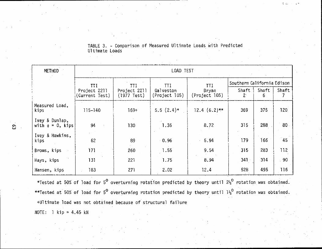
0'\ w

METHOD

TABLE 3. - Comparison of Measured Ultimate Loads ~ith Predicted Ultimate Loads

LOAD TEST

TTI TTI TTI TTI Southern ca 1 i forn i a Edison Project 2211 Project 2211 Galveston Bryan Shaft Shaft Shaft

(Current Test) (1977 Test) (Project 105) (Project 105) 2 6 7

Measured Load, kips 115-140 169+ 5.5 (2.4)* 12.4 (6.2)** 369 375 120

Ivey & Dunlap, with <P = 0, kips 94 130 1.35 8.72 315 288 80

Ivey & Hawkins, kips 62 89 0.96 5.94 179 166 45

Broms, kips 171 260 1. 55 9.54 315 283 112

Hays, kips 131 221 1. 75 8.94 341 314 90

Hansen, kips 183 271 2.02 12.4 528 495 116 - ---- -- - ----~---· -- ---- --- -- -----

*Tested at 50% of load for 5° overturning rotation predicted by theory until 2~0 rotation was obtained.

**Tested at 50% of load for 5° overturning rotation predicted by theory until 1~0 rotation was obtained.

+Ultimate load was not obtained because of structural failure

NOTE: 1 kip = 4.45 kN

',,

I I

-I

These two tests.cannot be compared in the same way as the other

tests because these shafts were loaded with a constant lateral load over

an extended period of time. However, it is interesting to note that the

Galveston and Bryan tests reached a rotation of 1~0 and 2~0 respectively,

for the 50% ultimate load.

Dunlap and Ivey (ll) stated that the use of this percentage (50%)

for long-term loads would probably result in significant rotations, and

the engineer should decide what rotation is acceptable for a particular

structure. It was also mentioned that if the rotation is limited by

functional or aesthetic considerations the use of smaller rotations and

loads may be necessary. It should be pointed out that for these two

tests (Galveston and Bryan) along with the 15 model tests by Hays et al.

(13) that the load was applied at a distance above the ground surface of

approximately twice the buried depth of the test shaft. In addition, the

depth to diameter ratios were much smaller than the TTI project 211

studies and the Southern California tests.

This information see.ms to indicate that as the depth to diameter.

ratio decreases, the Hays method predicts values which are more conserva­

tive than for large'r ratios. This may pos.sibly be due to the fact that

the equation which Hays uses for soil reaction is conservative near the

surface. Therefore, a better correlation may be obtained using the Hays

method if the ultimate soil reaction predicted near the surface is

increased.

The Ivey and Hawkins (17) method as shown in Table 3 which is based

on the Rankine passive earth pressure theory consjstently yields con­

servative predictions. This conservatism is also indicated in Fig. 29

64

" 4

since the measured ultimate soil reaction for the present study exceeds

the Rankine predicted so'il reaction. The method by Ivey and Dunlap is a

semi-empirical method which involves the use of a modifying factor that

is applied to the Rankine coefficients of passive and active earth

pressures. The modifying factor is applied in the use of both the

cohesive shear str~ngth and the angle of shearing re~istance when deter-

mining the ultimate load of a foundation. In order to calculate the

predicted values presented in Table 3, the angle of shearing resistance

was assumed to be equal to zero and the undrained shear strength was used

as reported by the authors. This method (Ivey and Dunlap) seems to

work well for small lateral loads but becomes more conservative for the

larger lateral loads.

The method proposed by Broms (4) gives predicted loads which are

reasonably close to the measured value in some cases. However, there is

not a consistent trend in the predicted ultimate loads. Some predicted

loads are conservative while others are unconservative. One very

significant point concerning the Broms method is that the unit weight

of the soil is not used anywhere in the calculations. All the other

m~thods presented in Tabie 3 include the use of.the unit weight of the·

soil along with the undrained shear strength, Cu, for calculating the

ultimate load on a drilled shaft.

The method which Hansen proposes seems to give predicted loads

which are generally unconservative but in a few cases the predicted

loads are close to the measured loads. The Hansen method is not easily

adaptable to a chart solution but requires only a few iterations for an

ultimate load to be obtained. The earth pressure coefficient for

65

cohesion which is used in determining the soil reaction incorporates both ,,

the angle of shearing resistance and depth to diameter ratio. These

factors are not included in all the other methods presented in Table 3

for calculating the soil reaction. Three of the methods (Ivey and Dunlap,

Broms, and Hays) seem to give predicted values of ultimate lateral load

which are close to each other and to the measured values. Therefore,

any of the three methods could be used for design purposes, as long as

a safety factor is included for added assurance that failure will not

occur. However, since the Hays method does seem to correlate best with

the load tests presented in Table 3, this method will be used, with a

slight modification, as the recommended preliminary design criteria for

this current study.

66

PRELIMINARY DESIGN PROCEDURE

It is considered appropriate to use rigid foundation design p,ro­

cedures when designing drilled shafts to support precast panel retaining

walls. There are several reasons for using the rigid design procedure.

In the first place the lateral loads on most retaining walls should not

be of such large magnitude as to necessitate a deeply embedded shaft

that would require elastic analysis. Secondly, in most instance_s rigid

design procedures are less complicated than elastic solutions because

they do not require computer solutions. However, to be reasonably

assured of rigid foundation behavior, the depth over diameter ratio of

the drilled shaft should be limited to six (19, 38).

There are several other design parameters which must be obtained

before the depth and diameter of a shaft supporting a retaining wall can

be determined. These parameters include the resultant force acting on

the retaining wall, the point of application of the resultant force, the )

undrained shear strength of the soil, the allowable shaft rotation, and

the creep potential of the soil.

Force· Acting, on Retaining Wall

The force acting on a retaining wall is the resultant of the lateral

pressure in the backfill. Based on the results of a study conducted on

an instrumented precast panel retaining wall, Wright et al. (39)

developed an equation to predict the resultant force of a level,

cohesionless backfill with no surcharge, acting on a retaining wall. The

equation developed to predict this is:

Fr = 0.25 yh2L (Ka + 0.8) .. (6)

67

where his the height of the wall and Lis the length of the panel,

pilaster to pilaster. The term y has been defined in Eq. T (p. 59).

The expression for Ka is the Rankine coefficient of active earth

pressure, and is defined as follows:

COS/; -

Ka = cosz; (7)

cos z; +

where z; is'the angle of the slope of the backfill to the horizontal

and ~· is the effective angle of shearing resistance of the backfill

material.

Application Point of Resultant Force

Wright et al. also developed an equation to calculate the location

of the point of application of the resultant force, Fr, of a level back­

fill with no surcharge. The equation is:

H = !!. OKa + 0. 26;l 2 Ka + 0.8 ~ · (8)

where H is the distance from the ground surface to the point where the

force is applied above the base of the retaining wall. The terms hand

Ka were defined in Eqs. 6 and 7.

Soil Shear Strength

The State Department of Highways and Public Transportation often

uses the Texas Cone Penetrometer Test as the primary means of deter­

mining soil shear strength in routine subsurface investigations.'

68-'

Laboratory testing to determine soil shear strength is often omitted

because of the additional expense involved. The TCP test consists of

driving a 3.0in. (7.6 em) diameter cone attached to a drill rod, with a

170 lb (77.1 kg) hammer. The hammer is dropped 2ft (0.61 m) for each

blow. The cone is seated with 12 blows and the number of blows, ~·

required to produce the next foot of penetration is recorded (10).

An improved correlation between the TCP blow count, N, and the

undrained shear strength has recently been reported by Duderstadt et al.

(10). The correlation has been reported for highly plastic homogeneous

clays (CH) and for homogeneous clays of low to medium plasticity (CL).

The results were reported as:

Homogeneous CH Cu = 0.067N

Homogeneous CL Cu = 0.053N

(9)

(1 0)

If it is desired by the designer a factor of safety may be applied to

the shear strength, Cu.

Allowable Shaft Rotation

If excessive rotation of the drilled shaft were allowed to occur,

objectionable deflection of the panel retaining wall in terms of

aesthetics and possibly serviceability would result. It is therefore

desirable to incorporate a factor of safety to guard against this

potential problem.

Based on the finding that the ultimate load of a rigid shaft for

minor service structures generally occurs at a rotation of 5°, Ivey and

Dunlap (16) proposed that the following equation be used as a factor of

69 '

safety against undesirable rotation:

Fr . Pe = 2 • • . . . . . . . . . . . • . • • . •

1 _ ( 5-e) 25

( 11)

where Fr is the resultant force transmitted from the wall to the shaft

(from Eq. 6) and e is the desired limiting angle of rotation. P8

is

the force acting at height, H, necessary to rotate the shaft through the

limiting angle of rotation, e. However, the results of this current

study indicate that the 5° rotation limit is too large for drilled shafts

supporting precast panel retaining walls and is not applicable for this

case as it was in the case of foundations of minor service structures.

Therefore, it is proposed that the 5° rotation limit be changed to a

value of 2.5° rotation. Thus, the equation to be used for factor of

safety against undesirable rotation is as follows:

Fr Pe = (2.5-e)2

1 - ~T--;~-6.25

(12)

The amount of rotation producing undesirable lateral deflection is ' '

dependent not only upon the size and configuration of the wall but also

upon th~ location. It was observed during this study that a total

rotation of as much as 2° could be aesthetically objectionable. The

total rotation actually consists of two separate movements after the

lateral load is applied. The first is the initial rotation that occurs

immediately after the application of the load. The second is a long-

term rotation that occurs as a result of soil creep. In view of these

considerations it is recommended that e be limited to 1° rotation or

' 70: ',

less.

Soil Creep

The time-dependent deformation behavior of a soil mass under a

given set of sustained stresses is referred to as creep. There are many

factors which probably contribute to creep in soils, but, each specific

factor which influences the amount of creep is not completely known or

understood. It is generally agreed that creep is a function of several

variables including, soil type, soil structure, seasonal variation in

temperature and moisture content, and stress history (6, 11). Therefore,

the soil in contact with the drilled shaft supporting the panel wall will

be subjected to the creep phenomena due to the sustained load being ;

applied to the wall.

Dunlap et al. (11), in a study of sustained loads on drilled shafts,

recommended that a factor of safety based on the soil type be applied to

account for creep. A factor of safety of 3 is recommended for soft and

stiff fissured clays. For stiff non-fissured clays, a factor of safety

of 2 is recommended. It was stated that although these safety factors

should result in a rotation that terminates, it is 1ikely.that the

rotation will be significant and in the order of 1°. Therefore, if an

appropriate safety factor for creep is used in conjunction with a

limiting angle of rotation, e equals 1° or less, it is likely that the

total shaft rotation will be limited to 2° or less.

Drilled Shaft Design Method

Based on the data presented in Table 3, the method proposed by Hays

71·

has been selected as the preliminary design method. However, a modifi­

cation of the ultimate soil reaction at the ground surface, Puo' will be

incorporated into the Hays method. This modification will involve an

increase from a value of 2.0 to 2.25 for the constant multiplied by the

undrained shear strength, Cu' and the diameter of the shaft, B (see

Eq. 5). In order to expedite the design procedure, a dimensionless

design chart deve 1 oped by Hays ( 13) wi 11 be used as presented in Fig. 33.

Since it is impossible to depict accurately all data with a family of

curves, it may be necessary to develop additional data points. Also, a

computer could be used to determine the exact ratio of S/Pu0D needed in

the solution for the ultimate lateral load, Su. This would minimize the

possibility of error introduced by interpolating. These points can

be generated by using the fo 11 owing_ two equation:

S I p D = 2 K - 1 + 8 ( K2 - • 5) U U0

( 13)

(S /p D)(H/0) = -K2 + .5 s/3 (2K3 - 1) U U0

( 14)

K is the ratio of x over D and f3 is a nondimensional variable

expressed as the slope of the soil _reaction curve times the diameter, B,

and divided by the depth of the shaft, D. s is the ultimate lateral u

load and H, x and p have been defined previously. Eq. 13 can be Uo

solved for K with selected values for both S /p D and f3. K can then be U U0

substituted into Eq. 14 and the ratio of H/0 is obtained. This procedure

may be fo 11 owed for different va 1 ues of S /p D with f3 being constant · U U0

until a complete solution is obtained.

J

"

0

~ a:: 0

0 ::J .e-

::::s

0.9---..,-----...,._..--...,._..--~-----r-----,

U) 0.4l----l.-+4-~~~4r-~-+----+----+-----f

0.0'----..1...-----'-----'-----'----...L------J 0.0 0.5 1.0 1.5 20 2.5 3.0

HID RATIO

FIG. 33- DESIGN CHART FOR COHESIVE SOILS (AFTER HAYS)

73 ..

Proposed Design Procedure

The following procedure is recommended as the preliminary design

method for the design of drilled shafts to support precast panel retain­

ing walls:

1. Use Eq. 6 to calculate the force, Fr, that will be applied to

the shaft by the retaining wall.

2. Use Eq. 8 to calculate the point of application, H, of the

force, Fr.

3. Set e equal to 1° or less and calculate the resulting force,

p8

, using Eq. 12

4. Choose the appropriate factor of safety for soil creep and

calculate the design force pd as: pd = p8

(F.S.)

5. Determine the undrained ~.hear strength, Cu, of the

soil by use of Eq. 9 or 10. A factor of safety may be

applied if desired.

6. Choose a trial value for shaft diameter, B, and embedment

depth, D.

7. Calculate xr using the following operation:

xr = 7 C B/(yB + .5 C ) u u

8. Calculate a using the fo 11 owing equations:

7C B a = --fj- for D > xr

7C B a= _u_ for

xr D < xr

9. Solve. for the soil reaction, puo' at the surface using the

following equation:

p = 2.25 C B U0 U

10. Calculate s using the following equation:

11. Determine the ratio of the height of .the applied force, H, to

the depth o.f the shaft, D.

12. Enter the design chart (Fig. 33) with s and H/D to obtain the

ratio S /p D. U U0

13. Multiply the ratio S /p D by p D to obtain the ultimate U U 0 U 0

lateral load, Su.

14. Repeat Steps 6-13 until the value calculated for Su exceeds the

design force, pd, calculated in Step 4 by a minimum amount.

Example of Design Procedure

The following example is provided as an aid in the design of precast

panel retaining wall foundations. A drilled shaft foundation is· to be

designed for the following situation:

A retaining wall is to consist of panels having a depth of 10 ft

(3.05 m) and length of 12ft (3.7 m). The backfill material will be

clean sand having an effective angle of shearing resistance, ~·, equal to

36° and unit weight, y, equal to 115 pcf (18.1 kN/m3). The backfill

will have no additional surcharge and will have a horizontal slope. The

subsoil at the construction site has been classified as a non-fissured

75

CH. The average N value obtained from the TCP test conducted at the

site is 20. The unit weight of the subsoil is 130 pcf (20.4 kN/m3).

The limiting angle of rotation, e, is 1°.

Step la using Eq. 7:

Ka = cos 0° = 0.260

Step lb using Eq. 6:

Fr = 0.25 (.115)(10) 2(12)(0.260 + 0.8) = 36.6 kips

Step 2 using Eq. 8:

H = lQ [0.260 + 0.267l = 2. 49 ft 2 0.260 + 0.8 J

Step 3 using Eq. 12:

P = 36 · 6 = 57.19 kips 1 - (2.5- 1)2

6.25

Step 4: Calculate Pd; soil conditions indicate that F.S. = 2.0.

Pd = 57.19 (2) = 114.38 kips

Step 5:

Step 6:

Try:

C = (0.067)(20) = 1.340 TSF = 2.68 KSF u .

Choose trial depth, 0, and diameter, B.

B = 3 ft

D = 15 ft

76

Step 7: Calculate xr:

X = 7<2·68)( 3) = 32 53 ft r .130(3) + .5(2.68) · ·

Step 8: Calculate a; the slope of the soil reaction curve:

since D < xr then

a _ 7(2.68)(3) = 1 73 - 32.53 .

Step 9: Calculate p ; the soil reaction at the surface: Uo

Puo = 2.25 (2.68)(3) = 18.09 k~ls

Step 10: Calculate s: s = (1.73){15) = 1 43

18.09 .

Step 11: Divide the distance to the point of application of the

resultant force on the wall by the depth of shaft:

!:! = 2.49 = 17 D 15 .

Step 12: From the Design Chart (Fig. 33):

s _.!!_D = .49 Pu

0

Step 13: Solve for the ultimate load:

Su = (.49)(18.09)(15) = 133.0 kips

133.0 > 114.4 :. This solution is valid. However,

a more optimum design may exist.

77

Repeat Steps 6 - 13.

Step 6: Choose a new trial depth, D, and diameter, B:

Try B = 3 ft

D = 14 ft

Step 7: Calculate Xr:

- 7 ( 2 . 68 )( 3) xr- .130(3) + .5(2.68) = 32.53 ft

Step 8: Calculate a:

since D < Xr then

= 7(2.68)(3) = 1 73 a 32.53 ·

Step 9: Calculate p : Uo

p = 2.25(2.68)(3) = 18.09 kips Uo

Step 10: Calculate s:

13 = {1. 73}(14} = 1.34 18.09

Step 11: H 0

2.49 = 18 14 .

Step 12: Using Design Chart:

78

Step 13: Solve for Su

Su = (.48)(18.09}(14) = 121.6 kips

121.6 > 114.4 This solution is also valid.

There may still exist a more optimum design, but the value calculated

is close enough to the required value to perform satisfactory with an

added assurance of safety. Therefore choose the 3-ft diameter by 14-ft

depth shaft.

79

CONCLUSIONS AND RECOM~ENDATIONS

The second year of a research study on the design of drilled shafts

to support precast panel retaining walls has been completed. Progress

has been made towards the improvement of design criteria for these

drilled shafts. Based upon the analysis of the data obtained from the

second lateral load test of an instrumented drilled shaft, the follow­

ing conclusions and recommendations are made:

Conclusions

1. Lateral deflections were of such magnitude near the end of

the testing program that they,would probably be aesthetically

objectionable. It is concluded that al.lowable deflection or

rotation rather than ultimate lateral load based on soil

failure may be the controlling factor for the design of

drilled shafts supporting precast panel retaining walls.

2. Based on the comparison of the measured versus predicted

ultimate loads given in Table 3, the Hays method does give

the best overall correlation of the different methods which

were investigated. Therefore, the Hays method with slight

modification is recommended for use as the preliminary design

procedure.

3. The Hays method, the Broms method, and the Ivey and Dunlap

method with ~ equal zero, all seem to predict values of

ultimate lateral load which are reasonable. Therefore, it

is concluded that any of these methods could be used if

appropriate safety measures are incorporated into the

80

particular design method chosen.

4. The Ivey and Hawkins design method, which is based on Rankine•s

passive earth pressure formula, constantly predicted values of

ultimate lateral load which were highly conservative. There­

fore this method is not recommended.

5. The Hansen method seems to define an upper bound of values for

ultimate lateral load and appear to be generally unconservative.

Therefore, this method is not recommended.

6. The available test data which have been published are limited

and the proposed preliminary design procedure· should be used

with caution. Therefore, some degree of conservatism is

suggested by using conservative values of the limiting angle

of rotation, e; the factor of safety applied to the undrained

cohesive shear strength, Cu; and the factor of safety applied

for soi 1 creep.

Recommendations

1. Additional ultimate load tests should be conducted on shafts.

of varying depths and diameters.

2. A comprehensive definition of ultimate load based on limiting

soil resistance and deformation is needed.

3. A limiting value for total deflection or rotation of a drilled

shaft supporting a precast panel retaining wall should be

determined.

4. Sustained lateral load tests should be conducted on shafts o.f

varying depth and diameters in order to study the creep

81

phenomenon.

5. Other lateral load tests should be conducted in other soil

types such as sand and silt.

82

APPENDIX I - REFERENCES

1. Adams, J. I., and Radhakri shna, H. S., 11 The Latera 1 Capacity of Deep Augered Footings, .. Proceedings, Eighth International Conference on Soil Mechanics and Foundation Engineering, Vol. 2.1, Mockba, USSR, 1973, pp. 1-8. .

2. Bhushan, Kul, Haley, Steven C., and Fang, Patrick T., 11 Lateral Load Tests on Drilled Piers in Stiff Clays, .. Preprints 3248, ASCE Spring Convention and Exhibit, Pittsburgh, Pennsylvania, April 24-28, 1978.

3. Bowles, Joseph E., Foundation Analysis and Design, 1st. ed., McGraw-Hill Book Co., New York, 1968, pp. 503-512.

4. Broms, Bengt B., 11 Lateral Resistance of Piles in Cohesive Soils, .. Journal of the Soil Mechanics and Foundation Division, ASCE, Vol. 90, No. SM2, Proc. Paper 3825, March, 1964, pp. 27-63.

5. Broms, Bengt B., 11 Lateral Resistance of Piles in Cohesionless Soils, 11 Proceedings of the American Society of Civil Engineers, Journal of Soil Mechanics and Foundation Division, ASCE, Vol. 91, No. SM3, May 1965, pp. 79-99.

8. Davisson, M. T., and Gill, H. L., "Laterally Loaded Piles in a Layered Soil System, .. Journal of the Soil Mechanics and Foundation Division, ASCE, Vol. 89, No. SM3, Proc. Paper 3509, May 1963, pp. 63-94.

9. DuBose, Lawrence A., 11 A Comprehensive Study of Factors Influencing the Load Carrying Capacities of Drilled and Cast in Place Concrete Piles," Texas Highway Department Project No. RP-4, Texas Trans­portation Institute, Texas A&M University, July 1956.

10. Duderstadt, Frankl in J., Coyle, Harry M., and Bartoskewitz, Richard E., .. Correlation of the Texas Cone Penetrometer Test N-Value with Soil Shear Strength, .. Research Report 10-3F, Texas Transportation Institute, Texas A&M University; September 1970.

11. Dunlap, Wayne A., Ivey, Don L., and Smith, Harry L., 11 Long-Term Overturning Loads on Drilled Shaft Footings," Research Report 105-5F, Texas Transportation Institute, Texas A&M University, September 1970.

83

12. Hansen, J. Brinch, 11 Th,e Ultimate Resistance of Rigid Piles Against Transversal Forces, .. Danish Geotechnical Institute, Bulletin 12, 1961.

13. Hays, C. 0., Davidson, J. L., Hagan, E. M., and Risitano, R. R., 11 Drilled Shaft Foundation for Highway Sign Structures, .. Research Report D647F, Engineering and Industrial Experiment Station, University of Florida, December 1974.

14. Heijnen, W. J., and Lubking, P., ~Lateral Soil Pressure and Negative Friction on Piles, .. Proceedings, Eighth International

· Conference on Soi 1 Mechanics and Foundation Engineering, Vol . 2.1 , Mockba, USSR, 1973, pp. 143-147.

1!5. Ivey, Don L., 11 Theory, Resistance of a Drilled Shaft Footing to Overturning Loads, .. Research Report 105-l, Texas Transportation Institute, Texas A&M University, February 1968~

16. Ivey, Don L., and Dunlap, Wayne A., 11 Design Procedure Compared to Full-Scale Tests of Drilled Shaft Footings, .. Research Report 105-3, Texas Transportation Institute, Texas A&M University, February · 1970.

17. Ivey, Don L., and Hawkins, Leon, 11 Signboaq:! Footings to Resist Wind Loads, .. Civil Engineering, Vol. 36, No. 12, December 1966, pp. 34-35.

18. Ivey, Don L., Koch, Kenneth J., and Raba, Carl F., Jr., .. Resistance of a Drilled Shaft Footing to Overturning Loads, Model Tests and Correlation with Theory, .. Research Report 105-2, Texas Transporta­tion Institute, Texas A&M University, July 1968.

19. Kasch, Vernon R., Coyle, Harry M., Bartoskewitz, R. E., and Sarver, t~illiam G., 11 Design of Drilled Shafts to Support Precast Panel R~taining Walls, .. Research Report No. 211-1, Te~as Transportation Institute, Texas A&t~ University, November 1977.

20. Lytton, Robert L., 11 Design Charts for Minor Service Structure Foundations, .. Research Report 506-lF, Texas Transportation Institute, Texas A&M University, September 1971.

21. McClelland, Bramlette, and Focht, John A., Jr., 11 Soil Modulus for Laterally Loaded Piles, 11 Journal of the Soil Mechanics and Foundations Division, ASCE, Vol. 82, No. SM4, Proc. Paper 1081, October 1956, pp. 1081-1 - 1081-22.

22. Mason, H. G., and Bishop, J. A., 11 Measurement of Earth Pressure and Deflection Along the Embedded Portion of a. 40-ft Steel Pile, .. ASTM Special Technical Publication, No. 154-A, 1954, pp. 1-21.

23. Matlock, Hudson, .. Correlations for Design of Laterally Loaded Piles

84

in Soft Clay, .. Preprints, Second Annual Offshore Technology Conference, Paper No. OTC 1204, 1970, pp. 577-594.

24. Matlock, Hudson, and Reese, Lymon C., 11 Generalized Solutions for Laterally Loaded Piles, .. Journal of the Soil Mechanics and Foundation Division, ASCE, Vol. 86, No. SM5, Part I, Proc. Paper 2626, October 1960, pp. 63-91.

25. Osterberg, J. 0., 11 Lateral Stability of Poles Embedded in a Clay Soil , 11 Northwestern University Project 208, Bell Telephone Laboratories, Evanston, Illinois, December 1958.

26. Outdoor Advertising Association of America, Engineering Manual, Outdoor Advertising Association of America, Chicago, Illinois, 1955.

27. Prescott, David M., Coyle, Harry M., and Milberger, Lionel J., 11 Field Measurements of Lateral Earth Pressures on a Pre-Cast Panel Retaining Wall, .. Research Report No. 169-3, Texas Transportation Institute, Texas A&M University; September 1973.

28. Reese, Lyman C., Discussion of 11 Soil Modulus for Laterally Loaded Piles, 11 by Bramlette r.lcClelland and John A. Focht, Jr., Transaction~, ASCE, Vol. 123, 1958, pp. 1071-1074.

29. Reese, Lyman C., Cox, William R., and Koop, Francis D., 11 Analysis of Laterally Loaded Piles in Sand, .. Preprints, Sixth Annual Offshore Technology Conference, Paper No. OTC 2080, 1974, pp~ 473-483.

30. Reese, Lyman C., Cox, William R., and Koop, Francis D .. , 11 Field Testing and Analysis of Laterally Loaded Piles in Stiff Clay, 11

Preprints, Seventh Annual Offshore Technology Conference, Paper No. OTC 2312, 1975, pp. 671-690.

31. Reese, Lymon C., and ~4elch, R. C., 11 Lateral Loading of Deep Foundations in Stiff Clay, .. Journal of the Geotechnical Engineering Division, ASCE, Vol. 101, No. 677, Proc. Paper 11456, July 1975, pp. 633-699.

32. Seiler, J. F., 11 Effect of Depth of Embedment of Pole Stability, .. Wood Preserving News, Vol. 10, No. 11, November 1932, pp. 152-168.

33. Shilts, W. L., Graves, L. D., and Driscoll, G. G., 11 A Report of Field and Laboratory Tests on the Stability of Posts Against Lateral Loads, .. Proceedings, Second International Conference on Soil ~~echanics and Foundation Engineering, Vol. 5, Rotterdam, Holland, 1948, pp. 107-122.

34. Stobie, James C., 11 Pole Footings, .. Journal of, the Institute of Engineers, Australia, Vol. 2, 1930, pp. 58-63.

85

Terzaghi, Karl, and Peck, Ralph B., Soil Mechanics in Engineering Practice, 2nd ed., John Wiley & Sons, Ltd, New York, 1967, pp. 198-200.

I

36. Vesic, Aleksandar B., 11 Bending of Beams Resting on Isotropic Elastic Solid, 11 Journal of the Engineering Mechanics Division, ASCE, Vol. 87, No. EM2, Proc. Paper 2800, April 1961, pp. 35-53.

37. Welch, Robert C., and Reese, Lymon C., .. Lateral Load Behavior of Drilled Shafts, .. Research Report 89-10, Center for Highway Research, The University of Texas at Austin, May 1972.

38. Woodward, Richard J., Gardner, WilliamS., and Greer, David M., Drilled Pier Foundations, McGraw-Hill Bdok Co., New York, 1972, 287 pp.

39. Wright, William V., Coyle, Harry M., Bartoskewitz, Richard E., and Milberger, Lionel J., 11 New Retaining Wall Design Criteria Based on Lateral Earth Pressure Measurements, .. Research Report No. 169-4F, Texas Transportation Institute, Texas A&M University, August 1975.

86

APPENDIX II - NOTATION

The following symbols are used in this thesis:

B = foundation diameter;

Cu = undrained cohesive shear strength;

D = embedded depth;

Fr = resultant force transmitted from retaining wall to

drilled shaft;

H =height of lateral load application;

h =height of retaining wall;

Ka = Rankine coefficient df active earth pressure;

Kc = earth pressure coefficient;

L =length of precast panel;

N = blow count from TCP Test;

Pd =design force;

Pu = ultimate soil reaction at groundline; 0

P8

=force acting at height, H1, to rotate shaft through

angle;

p = soil reaction;

p = ultimate lateral soil reaction; u

WF = wide flange;

x = depth below groundline;

e = limiting angle of rotation;

s = nondimensional variable;

~ = angle of shearing resistance;

~· = effective angle of shearing resistance;

87

a = slope of the Hays soil re~ction curve

y = unit weight of overburden material

t - angle of slope of backfill to horizontal; and

n = soil strength reduction factor.

88

J. APPENDIX I II - EXPLANATION OF SPEClAL LOADING PROCEDURES

Due to the design of the loading system and its inherent operating

limitations, a constant lateral load was not maintained on the test

shaft over an extended period of time. By the time the load had

reached 115-kips (512 kN) it was apparent that for any given load

the movement was continuing for an indefinite period of time. At this

point in the loading procedure the decision was made to measure the

length of time the shaft would continue to move under a given load and

to determine if the movement would continue at a constant rate. This

additional information was needed to determine when it would be

reasonable to take representative pressure measurements and inclination

readings for a given load. Therefore, two different methods were used

in the loading procedure after the 120-kip (534-kN) level had been

attained. These two methods were designated the "Constant Time Interval

Method" and the "Average Load Method".

The Constant Time Interval Method consisted of two sets of measure­

ments during a fiv~ minute period. The first measurement was made as

soon as the load was reapplied and brought back up to the specified

reading on the Budd indicator. The second measurement was the total

movement of the shaft and was made at the end of the five-minute period.

These measurements were continued until it was felt that a constant

movement rate was obtained (even though the shaft was continuing to

move). These movements are shown in Tables III-1 thru III-5 for the

reapplication of load from the 120 kip (534 kN) level to that of the

130-kip {578 kN) reload level.

The Average Load Method consisted of setting the Budd indicator 50

89

TABLE III-1. -Deflections for Constant Time

Interval (Reload 120 kips)

Dial Reading Movement During

Time Time Time Increment 1 in. Load Interval

(Ni n.) Application Held

1140 0.986 5 0.924 0.062

1145 0.914 0.010

5 0.898 0. 016 1150 0.887 0.011

5 0.878 0.009

1155 0.866 0.012 0.858 0.008

NOTE: l kip = 4.45 kN; l in. = 2.54 em

90

Time

1210

1215

1220

1225

1230

1235

1240

TABLE III-2. - Deflections for Constant

Time Interval (Load 12b kips)

Dial Reading ~1ovement During Time Time

Increment 1 in. Load Interval (r~i n.) Application Held

0.834 5 0.798 0.036

0. 761 0.037 5 0.744 0.017

0.709 0.033 5 0.693 0.016

0.659 0.034 5 <·. 0.642 0.017

0.610 0.032 !) 0.598 0.012

0.573 0.025 5 0.558 . 0.015

0.531 0.027 0.522 0.009

NOTE : 1 kip = 4. 45 kN; 1 in. = 2. 54 em

91.

TABLE III-3. - Deflections for Constant Time

Interval (Reload 125 kips)

Dial Gage Readings Movement Du_ring

Tilile Time Time Increment 1 in. 5 in. Load Interval

(r1in.) Application Held

1105 6.372 3.842 5 0.296 3.780 0.076

1110 0.270 - 0.026 5 0.257 3.741 0. 013

1115 0.241 3.724 0.016 5 0.227 3.710 0.014

1120 0~215 3.698 0.012 5 0.206 3.689 0,009

1125 0.196 3.679 0.010 5 0.186 3.668 0.010

1130 0.176 3.658 0.010 5 0.168 3.649 0.008

1135 0.157 3.639 0. 011 I

NOTE: l kip = 4. 45 kN ; l in. = 2. 54 em

92

TABLE III-4. - Deflections for Constant Time Interval (Load 130 kips)

Dial Gage Readings Hovement During

Time Load Time

Time Increment 1 in. 5 in. Application Interval (t4in.) Held

1156 0.926 3.625

1153 0.898 3.598 0.028

1205 0.868 3.568 0.030

5 0.848 3.547 0.020

1210 0.834 3.530 0.014

5 0.819 3.513 0.015

1215 0.805 3.499 0.014

5 0.789 3.484 0.016

1220 0.776 3.469 0.013

5 0.760 3.452 0.016

1225 0.743 3.436 0.017

5 0.730 3.422 0.013

1230 0. 714 3.406 0.016

5 o. 701 3.393 0.013

1235 0.683 3.376 0.018

5 0.671 3.364 0.012

1240 0.658 3.352 0.013

5 0.699 3.337 0.014

1245 0.630 -3.324 0.014

0.619 3.312 0.011

0.595 3.288 -

NOTE: 1 kip = 4.45 kN; 1 in. = 2.54 em

93

TABLE III-5. - Deflections for Constant Time

Interval (Reload 130 kips}

Dial Gage Readings Hovement During

Time Load Time Time Increment 1 in. 5 in. Application Interval

(!'lin.} Held

1103 0.478 3.176

1110 0.420 3.116 0.058

1115 5 0.405 3.100 0.015

5 0.392 3.086 0.013

1120 0.378 3.072 0.014

5 0.366 3.062 0. 012

1125 0.354 3.050 0.012

5 0.345 3.041 0.'009

1130 0.334 3.029 0.011

5 0.326 3.022 0.008

1135 0.317 3. 012 0.009

5 . 0.310 3.005 . 0. 007

1140 0.300 2.994 0.010

5 0.392 2.986 0.008

1150 0.277 2.972 0.015

0.264 2.959 0.013

NOTE: 1 kip = 4.45 kN; 1 in. = 2.54 em

94

"j

j

micro strains above the desired load and letting it drop to 50 micro

strains below the load before reapplying it again. The time for this to

occur and the measurement of the deflections between each application

was recorded and shown in Table III-6.

As expected, the movement between each reapplication of th~ load

was relatively constant, but the time between each increment was

beginning to increase along with the movement between each interval.

After two hours significant movements were still being observed at a

nearly uniform rate. It was concluded that at this point that the

deflection was both a function of the time the load was held and the

load itself.

95

-(l

TABLE III-6. - Deflections for + 50 Microstrain

Range (Reload 130 kips)

Dial Gage Readings ~1ovement During

Time Load Time Time Increment 1 in. 5 in. Application Interval

{r4i n. ) Held

1430 0.221 2.914 0.043

16 0.196 2 .. 889 0.025 1446 0.179 2.872 0.017

26 0.167 2.861 0. 012 1512 0.146 2.840 0.021

32 0.136 2.829 0. 010 1544 0.114 2.807 0.022

40 0.104 2.797 0.010 1624 0.079 2. 772 0.025

0~069 2.762 0~ 010

NOTE: 1 kip = 4.45 kN; 1 in. = 2.54 em

96

NOTES

97

0