technical report tr-2016-16 - university of wisconsin ...sbel.wisc.edu/documents/tr-2016-16.pdf ·...
TRANSCRIPT

Simulation-Based Engineering LabUniversity of Wisconsin-Madison
Technical Report TR-2016-16
Using the Complementarity and Penalty Methods for Solving
Frictional Contact Problems in Chrono:
Validation for the Cone Penetration Test
Micha l Kwarta and Dan Negrut
Version: March 24, 2017

Abstract
The numerical results of cone penetration test were presented and validated againstexperimental ones. Two different approaches for modeling the dynamics of granularmatter were used. The first one, discrete element method with penalty contact mod-eling (DEM-P) [1], is an approach usually used in e. g. granular flows or powdermechanics simulations. The second method, called DEM-C (from “complementarity”)is essential in fields like robotics and graphics [2]. In this approach the bodies cannotpenetrate due to the complementarity conditions. Even though the methods modelcontact with friction in two different ways, as well as they can be described by usingtwo very different sets of mechanical and numerical parameters, the results obtainedfrom the simulations were comparable. The validation study was enriched by the per-formance analysis. We also examined how sensitive the simulations were to the changesof certain parameters’ values and particles shape. To obtain the results, an open sourcesoftware package, called Chrono was used [3]. The source code of the model used inthe numerical experiments is available on-line.
Keywords: cone penetration test, penalty contact modeling, differential varia-tional inequality modeling, friction, contact
1

Contents
1 Laboratory Experiments 51.1 Overview . . . . . . . . . . . . . . . . . . . . . . . . . . . . . . . . . . . . . . 51.2 Results . . . . . . . . . . . . . . . . . . . . . . . . . . . . . . . . . . . . . . . 8
2 Numerical Simulations 122.1 Physical Side of the Simulations . . . . . . . . . . . . . . . . . . . . . . . . . 122.2 Numerical Side of the Simulations . . . . . . . . . . . . . . . . . . . . . . . . 142.3 Results . . . . . . . . . . . . . . . . . . . . . . . . . . . . . . . . . . . . . . . 152.4 Performance analysis . . . . . . . . . . . . . . . . . . . . . . . . . . . . . . . 21
3 Additional Analyses 243.1 Impact of the µparticle-particle on the results . . . . . . . . . . . . . . . . . . . . 243.2 Impact of the µparticle-cone on the results . . . . . . . . . . . . . . . . . . . . . 273.3 Granular material made of the “double-spheres”. The sensitivity analysis of
the longitudinal dimension . . . . . . . . . . . . . . . . . . . . . . . . . . . . 30
4 Conclusion 33
2

Nomenclature
Abbreviations
DEM-P Discrete Element Method - Penalty
DEM-C Discrete Element Method - Complementarity
CPT Cone Penetrometer Test
LVDT Linear Variable Differential Transformer
Mathematical notation
N(µ, σ2) Normal distribution with mean µ and variance σ2
Physical parameters
Y Young’s modulus
ν Poisson’s ratio
% density
g Earth’s gravity
a average value of the upward acceleration caused by the friction force between the LVDTapparatus’ rod and its track, a = 2.21m
s2
µp−p inter-sphere coefficient of friction
µp−w coefficient of friction between particles and container’s walls
µp−c coefficient of friction between particles and cones
cr,p−p inter-sphere coefficient of restitution
cr,p−w coefficient of restitution between particles and container’s walls
cr,p−c coefficient of restitution between particles and cones
L30◦ height of the cone with 30◦ in apex angle, L30◦ = 34.36 mm
W30◦ width of the base’s diameter of the cone with 30◦ in apex angle, W30◦ = 9.21 mm
L60◦ height of the cone with 60◦ in apex angle, L60◦ = 22.10 mm
W60◦ width of the base’s diameter of the cone with 60◦ in apex angle, W60◦ = 19.86 mm
H height (relative to the granular material surface) the cones were dropped from;H ∈ {0, 1
2Li, Li}, i ∈ {30◦, 60◦}
3
Numerical parameters
∆t time step
MNoI maximum number of iterations
CRS contact recovery speed
4
1 Laboratory Experiments
1.1 Overview
The detailed report concerning the laboratory cone penetration test can be found in [4]. Inthis section aspects of the experiment which needed to be considered during the numericalmodeling were described. The mechanical and geometrical parameters of the bodies used inthe empirical tests were provided. The impact of the experimental apparatus on the resultswas briefly described as well.
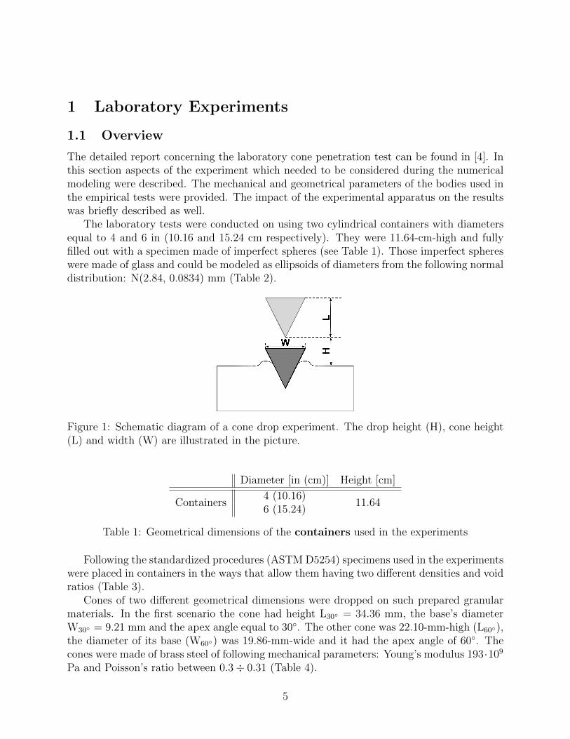
The laboratory tests were conducted on using two cylindrical containers with diametersequal to 4 and 6 in (10.16 and 15.24 cm respectively). They were 11.64-cm-high and fullyfilled out with a specimen made of imperfect spheres (see Table 1). Those imperfect sphereswere made of glass and could be modeled as ellipsoids of diameters from the following normaldistribution: N(2.84, 0.0834) mm (Table 2).
Figure 1: Schematic diagram of a cone drop experiment. The drop height (H), cone height(L) and width (W) are illustrated in the picture.
Diameter [in (cm)] Height [cm]
Containers4 (10.16)
11.646 (15.24)
Table 1: Geometrical dimensions of the containers used in the experiments
Following the standardized procedures (ASTM D5254) specimens used in the experimentswere placed in containers in the ways that allow them having two different densities and voidratios (Table 3).
Cones of two different geometrical dimensions were dropped on such prepared granularmaterials. In the first scenario the cone had height L30◦ = 34.36 mm, the base’s diameterW30◦ = 9.21 mm and the apex angle equal to 30◦. The other cone was 22.10-mm-high (L60◦),the diameter of its base (W60◦) was 19.86-mm-wide and it had the apex angle of 60◦. Thecones were made of brass steel of following mechanical parameters: Young’s modulus 193·109
Pa and Poisson’s ratio between 0.3÷ 0.31 (Table 4).
5
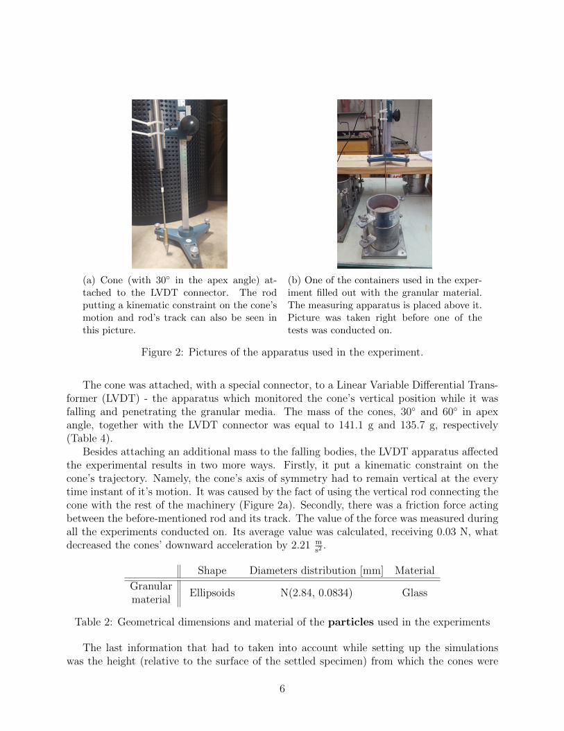
(a) Cone (with 30◦ in the apex angle) at-tached to the LVDT connector. The rodputting a kinematic constraint on the cone’smotion and rod’s track can also be seen inthis picture.
(b) One of the containers used in the exper-iment filled out with the granular material.The measuring apparatus is placed above it.Picture was taken right before one of thetests was conducted on.
Figure 2: Pictures of the apparatus used in the experiment.
The cone was attached, with a special connector, to a Linear Variable Differential Trans-former (LVDT) - the apparatus which monitored the cone’s vertical position while it wasfalling and penetrating the granular media. The mass of the cones, 30◦ and 60◦ in apexangle, together with the LVDT connector was equal to 141.1 g and 135.7 g, respectively(Table 4).
Besides attaching an additional mass to the falling bodies, the LVDT apparatus affectedthe experimental results in two more ways. Firstly, it put a kinematic constraint on thecone’s trajectory. Namely, the cone’s axis of symmetry had to remain vertical at the everytime instant of it’s motion. It was caused by the fact of using the vertical rod connecting thecone with the rest of the machinery (Figure 2a). Secondly, there was a friction force actingbetween the before-mentioned rod and its track. The value of the force was measured duringall the experiments conducted on. Its average value was calculated, receiving 0.03 N, whatdecreased the cones’ downward acceleration by 2.21 m
s2.
Shape Diameters distribution [mm] Material
GranularEllipsoids N(2.84, 0.0834) Glass
material
Table 2: Geometrical dimensions and material of the particles used in the experiments
The last information that had to taken into account while setting up the simulationswas the height (relative to the surface of the settled specimen) from which the cones were
6

(a) Cones with 60◦ and 30◦ in the apex angle. (b) Cones with LVDT connectors attached.
Figure 3: Pictures of the cones used in the experiment.
dropped. In the static cone penetration test, the cone was placed on the surface of thegranular material at zero drop height. In the dynamic loading, the cone was dropped atseveral heights above the surface of the granular material. The laboratory test of the dynamicloading was conducted for two different initial heights of cones. First one, was equal to thedropped cone’s height (L30◦ = 34.36 mm, L60◦ = 22.10 mm), and the other one equal to thehalf of its height (1
2L30◦ = 17.18 mm, 1
2L60◦ = 11.05 mm).
Density[kgm3
]Void Ratio
Loose Case 1504.32 0.66Dense Case 1630.35 0.53
Table 3: Densities and void ratios of specimens used in the empirical tests
ApexHeight [mm]
Base’sY [Pa] ν mass∗ [g]
angle Diameter [mm]
Cones30◦ 34.36 9.21
193 · 109 0.3÷ 0.31141.1
60◦ 22.10 19.86 135.7
Table 4: Geometrical dimensions and mechanical parameters of the cones used in the ex-periments∗ mass of the cones together with the LVDT connector
7

1.2 Results
Below, the experimental results presented in [4] were showed.
Figure 4: Depth/height vs. time plots of the cone 30◦ in apex angle. Container with a 4-inches-wide diameter. Granular material packed loosely.
Figure 5: Depth/height vs. time plots of the cone 30◦ in apex angle. Container with a 4-inches-wide diameter. Granular material packed densely.
8

Figure 6: Depth/height vs. time plots of the cone 30◦ in apex angle. Container with a 6-inches-wide diameter. Granular material packed loosely.
Figure 7: Depth/height vs. time plots of the cone 30◦ in apex angle. Container with a 6-inches-wide diameter. Granular material packed densely.
9

Figure 8: Depth/height vs. time plots of the cone 60◦ in apex angle. Container with a 4-inches-wide diameter. Granular material packed loosely.
Figure 9: Depth/height vs. time plots of the cone 60◦ in apex angle. Container with a 4-inches-wide diameter. Granular material packed densely.
10
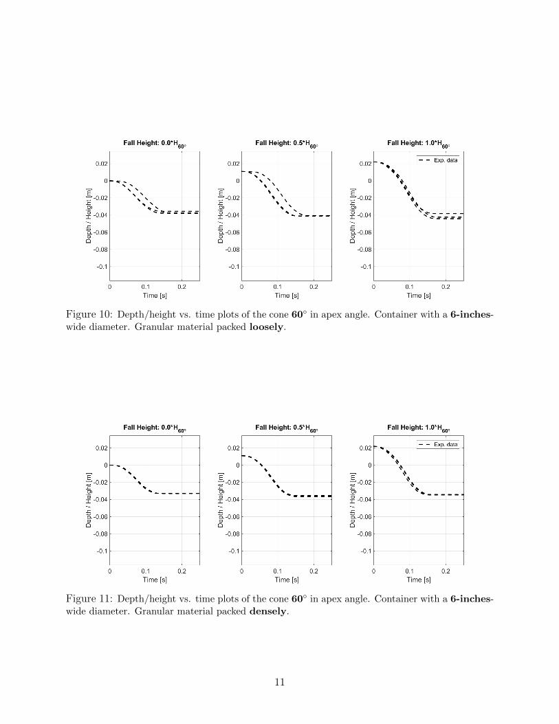
Figure 10: Depth/height vs. time plots of the cone 60◦ in apex angle. Container with a 6-inches-wide diameter. Granular material packed loosely.
Figure 11: Depth/height vs. time plots of the cone 60◦ in apex angle. Container with a 6-inches-wide diameter. Granular material packed densely.
11

(a) (b)
Figure 12: Kinetic energy of the mechanical system during the settling stage. Simulation withcontainer of diameter equal to (a) 4 inches (b) 6 inches.
2 Numerical Simulations
2.1 Physical Side of the Simulations
The simulations could be divided into two stages. In the first one (settling stage) the speci-men was poured into the container and was allowed to gain its equilibrium state (Fig. 12).The second one (cone penetration stage) was about placing the cone right above the surfaceof the granular material and dropping it with an initial vertical velocity equal to
√2(g-a)H,
where:
g was a gravity of Earth,
a was the average upward acceleration caused by the friction force between the LVDTapparatus’ rod and its track, a = 2.21m
s2and
H was one of the three initial heights the cone was dropped from (H ∈ {0, 12Li, Li},
i ∈ {30◦, 60◦})
The containers of a diameter equal to 4 and 6 inches were filled out with the granularmaterial consisted of the perfect spheres. The particles, with diameter of 2.84 mm each, weremade of glass of the following mechanical parameters: density 2500 kg
m3 , Young’s modulus108 Pa (value lower than in reality for stability reasons) and Poisson’s Ratio 0.3. The coef-ficient of restitution between particles was set to 0.658 [5]. The walls of the container weremassless and had the mechanical parameters of the same values.
A few words of explanation are in order concerning the values of the friction coef-ficient between particles (µparticle-particle, µp-p) and between particles and containers’ walls(µparticle-wall, µp-w). Values of those parameters played significant role in obtaining loser anddenser packings of the settled specimen. Namely, when the coefficients of friction were set
12

Material %[kgm3
]Y [Pa] ν
GranularGlass 2500 108 0.3
material
Table 5: The values of particles’ mechanical parameters used in the simulations
to 0.7 the settled granular material had a density similar to the one obtained in the loosecase of the empirical test. The packing seen in the dense case scenario was achieved afterthe settling simulation with the frictionless particles and walls. In the second part of thesimulation (cone penetration test) the before-mentioned friction coefficients together withµparticle-cone (µp-c) were set to 0.7. The analysis of friction coefficient impact on the resultswas described in Sections 3.1 and 3.2. The values of friction coefficients for objects madefrom steel of glass were summarized in [6].
Material Apex angle Y [Pa] ν mass∗ [g]
Cones Brass Steel30◦
193 · 109 0.3141.1
60◦ 135.7
Table 6: The values of cones’ mechanical parameters used in the simulations
Cones used in the simulations were given the geometrical dimensions and mass presentedin the Table 4. They were made of brass steel and were given the following parameters:Young’s modulus 193 · 109 Pa, Poisson’s ratio 0.3. The coefficient of restitution and coeffi-cient of friction between the steel cone an glass beads were equal to: 0.597 [5] and 0.7 [6],respectively.
A kinematic constraint was put on the cone to model the impact of the rod it was attachedto. With such constraint cone’s symmetry axis remained vertical at the every time instant.
Settling µp−p µp−w cr,p−p cr,p−w
Loose Case 0.7 0.70.658 0.658
Dense Case 0.0 0.0
CPT Test µp−p µp−w cr,p−p cr,p−w µp−c cr,p−c
Both Cases 0.7 0.7 0.658 0.658 0.7 0.597
Table 7: The values of mechanical parameters describing contacts used in the simulations
13

Approach time step [s] MNoI∗ CRS∗∗ [ms]
DEM-P 10−5 - -DEM-C 10−4 50 1.0
Table 8: Numerical parameters’ values used in the simulations∗ MNoI - maximum number of iterations∗∗ CRS - contact recovery speed
2.2 Numerical Side of the Simulations
To simulate the cone penetration test the mechanical system was modeled using two differentmethods of handling the friction and contact forces between colliding bodies: penalty (DEM-P) and complementarity (DEM-C) method. Those approaches can be successfully used insimulating the mechanical phenomena. If calibrated correctly, simulations based on DEM-P,as well as on DEM-C should give the results that are close enough to empirical measurementsand also to each other. Correct calibration is equal to choosing the numerical values for theparameters the two approaches can be characterized with from the numerical point of view.Those values should provide stability of the computations and model the physics sufficientlywell.
Stability of calculations in DEM-P model can be ensured by choosing the correct values ofthe time step (∆t). While using DEM-C method the combination of the following parameters:time step, contact recovery speed (CRS) and maximum number of iterations (MNoI) isimportant.
In both modeling approaches ∆t is the parameter responsible for the stability of calcu-lations. Too large value of the time step will make the simulations unstable, too small - willresult in having very long execution time. The optimal value of ∆t can be chosen using trialand error method. When it comes to the simulations run so far, the values of the time stepused in the simulations based on the DEM-C usually were about 10 times larger than inDEM-P-based ones.
Contact recovery speed (CRS) is a parameter used only in DEM-C-based simulations. Asits name indicates, it is a parameter that puts the upped limit on the normal component ofthe velocity two colliding bodies rebound off each other with. In complementarity approachthe bodies are modeled as they were rigid. Even though, at the beginning of each time stepbodies can overlap, assigning the penetration depth to such contact. In each time step, thenormal component of the velocity two bodies will rebound off each other is equal to thepenetration depth divided by the time step. If the value of this component exceeds the valueof the upper limit (called contact recovery speed) it is simply clamped to the value of thislimit. In other words, CRS provides stability to the simulations and allows having largervalues of ∆t and at the same time smaller amount of maximum number of iterations pertime step (MNoI). Thus, it also makes the execution time of the simulations shorter.
MNoI sets the maximum number of iterations that are done during each time step to cal-culate the values of the normal and tangential components of forces related to every contact.
14

(a) (b)
Figure 13: Cone penetration test - numerical setup: (a) cone placed over the settled specimen; (b)cone penetrating the granular material.
The value of this parameter depends on the type of the simulations. In the simulation of conepenetration test (CPT) 50 iterations per time step were enough to have reasonable results.Calculations with MNoI set up to 600 gave the satisfactory results concerning shear test [7].The simulations of standard triaxial test required the value of MNoI to be set to 2500, tohave calculation that were not only stable but also giving results correct from the physicalpoint of view [8]. The values of the above-described parameters used in the simulations ofcone penetration test were presented in Table 8.
2.3 Results
In this section the results obtained from the simulations were presented and compared to theexperimental data. The densities and void ratios of the samples in their equilibrium statewere summarized in the Tables from 9 to 12. The relative error between the simulations andempirical test varied from 1.19 % to 5.20 % concerning densities and from 3.85 % to 13.79 %when it comes to the void ratios. The displacements of the cones as functions of time wereplotted in the Figures from 14 to 21. The numerical results matched the experimental ones.Moreover, the outcomes from simulations based on DEM-P and DEM-C were comparable.It is noteworthy, taking into account the fact that those approaches model frictional contactdifferently and use different sets of parameters to describe physical phenomena.
15

Figure 14: Hight/depth vs. time plots of the cone 30◦ in apex angle. Container with a 4-inches-wide diameter. Granular material packed loosely.
Densities[kgm3
]Experiment
Simulation Relative Error [%]DEM-P DEM-C DEM-P DEM-C
Loose Case 1504.29 1449.59 1426.00 3.64 5.20Dense Case 1630.34 1608.79 1593.69 1.32 2.25
Table 9: A comparison of the experimental and numerical results. Densities of the samplesin their equilibrium state. Container with a diameter of 4 inches.
Densities[kgm3
]Experiment
Simulation Relative Error [%]DEM-P DEM-C DEM-P DEM-C
Loose Case 1504.32 1462.70 1433.39 2.77 4.72Dense Case 1630.35 1610.93 1601.22 1.19 1.79
Table 10: A comparison of the experimental and numerical results. Densities of the samplesin their equilibrium state. Container with a diameter of 6 inches.
16

Figure 15: Hight/depth vs. time plots of the cone 30◦ in apex angle. Container with a 4-inches-wide diameter. Granular material packed densely.
Void Ratios ExperimentSimulation Relative Error [%]
DEM-P DEM-C DEM-P DEM-C
Loose Case 0.66 0.72 0.75 9.50 13.79Dense Case 0.53 0.55 0.57 3.85 6.61
Table 11: A comparison of the experimental and numerical results. Void ratios of thesamples in their equilibrium state. Container with a diameter of 4 inches.
Void Ratios ExperimentSimulation Relative Error [%]
DEM-P DEM-C DEM-P DEM-C
Loose Case 0.66 0.71 0.74 7.15 12.43Dense Case 0.53 0.55 0.56 3.46 5.23
Table 12: A comparison of the experimental and numerical results. Void ratios of thesamples in their equilibrium state. Container with a diameter of 6 inches.
17
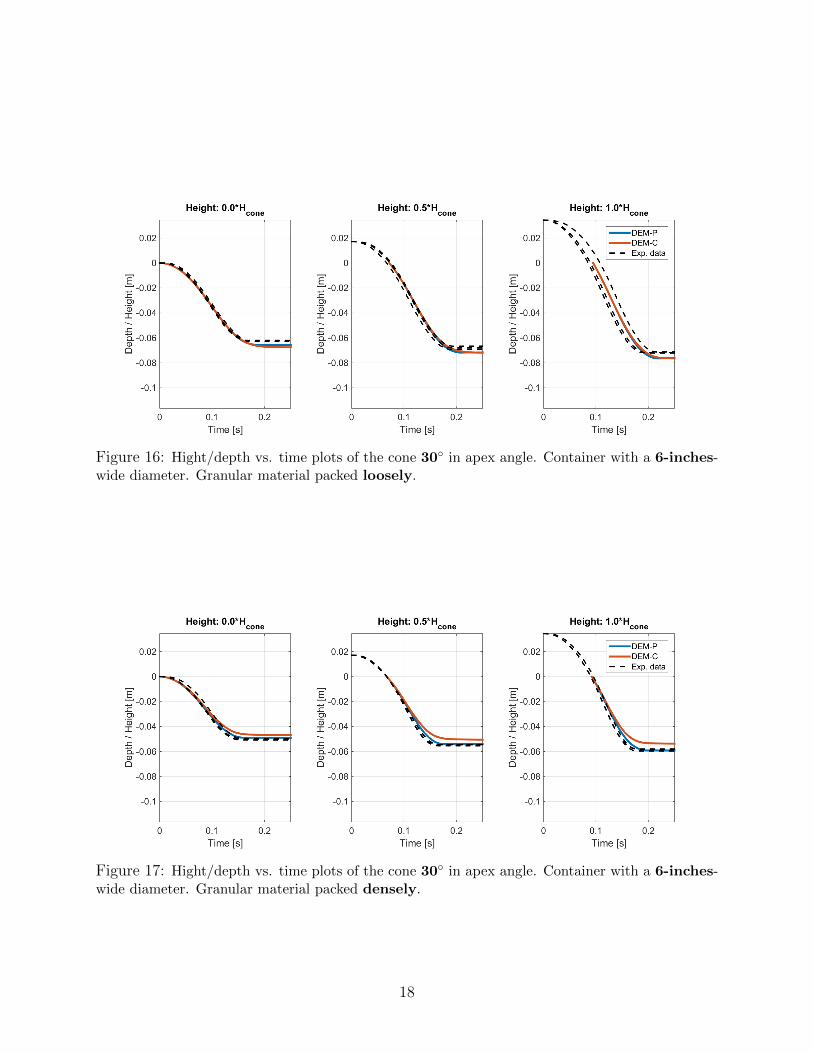
Figure 16: Hight/depth vs. time plots of the cone 30◦ in apex angle. Container with a 6-inches-wide diameter. Granular material packed loosely.
Figure 17: Hight/depth vs. time plots of the cone 30◦ in apex angle. Container with a 6-inches-wide diameter. Granular material packed densely.
18

Figure 18: Hight/depth vs. time plots of the cone 60◦ in apex angle. Container with a 4-inches-wide diameter. Granular material packed loosely.
Figure 19: Hight/depth vs. time plots of the cone 60◦ in apex angle. Container with a 4-inches-wide diameter. Granular material packed densely.
19
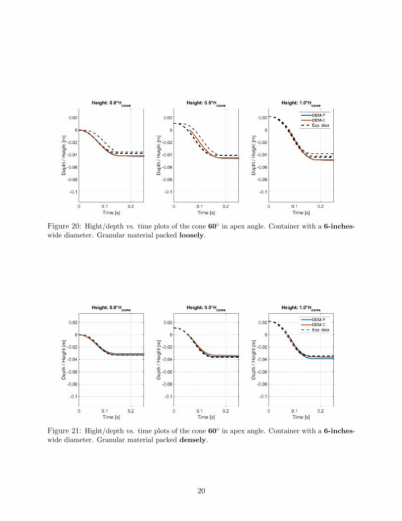
Figure 20: Hight/depth vs. time plots of the cone 60◦ in apex angle. Container with a 6-inches-wide diameter. Granular material packed loosely.
Figure 21: Hight/depth vs. time plots of the cone 60◦ in apex angle. Container with a 6-inches-wide diameter. Granular material packed densely.
20
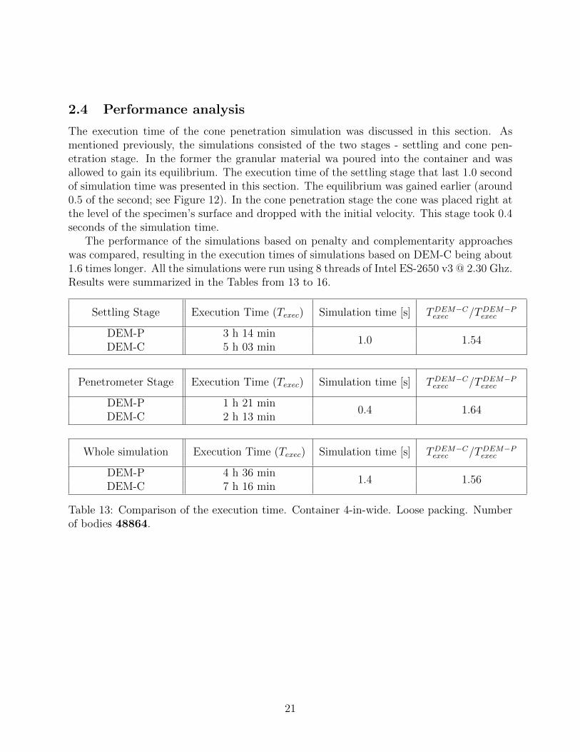
2.4 Performance analysis
The execution time of the cone penetration simulation was discussed in this section. Asmentioned previously, the simulations consisted of the two stages - settling and cone pen-etration stage. In the former the granular material wa poured into the container and wasallowed to gain its equilibrium. The execution time of the settling stage that last 1.0 secondof simulation time was presented in this section. The equilibrium was gained earlier (around0.5 of the second; see Figure 12). In the cone penetration stage the cone was placed right atthe level of the specimen’s surface and dropped with the initial velocity. This stage took 0.4seconds of the simulation time.
The performance of the simulations based on penalty and complementarity approacheswas compared, resulting in the execution times of simulations based on DEM-C being about1.6 times longer. All the simulations were run using 8 threads of Intel ES-2650 v3 @ 2.30 Ghz.Results were summarized in the Tables from 13 to 16.
Settling Stage Execution Time (Texec) Simulation time [s] TDEM−Cexec /TDEM−Pexec
DEM-P 3 h 14 min1.0 1.54
DEM-C 5 h 03 min
Penetrometer Stage Execution Time (Texec) Simulation time [s] TDEM−Cexec /TDEM−Pexec
DEM-P 1 h 21 min0.4 1.64
DEM-C 2 h 13 min
Whole simulation Execution Time (Texec) Simulation time [s] TDEM−Cexec /TDEM−Pexec
DEM-P 4 h 36 min1.4 1.56
DEM-C 7 h 16 min
Table 13: Comparison of the execution time. Container 4-in-wide. Loose packing. Numberof bodies 48864.
21

Settling Stage Execution Time (Texec) Simulation time [s] TDEM−Cexec /TDEM−Pexec
DEM-P 3 h 33 min1.0 1.67
DEM-C 5 h 55 min
Penetrometer Stage Execution Time (Texec) Simulation time [s] TDEM−Cexec /TDEM−Pexec
DEM-P 1 h 27 min0.4 1.76
DEM-C 2 h 32 min
Whole simulation Execution Time (Texec) Simulation time [s] TDEM−Cexec /TDEM−Pexec
DEM-P 5 h 00 min1.4 1.69
DEM-C 8 h 27 min
Table 14: Comparison of the execution time. Container 4-in-wide. Dense packing. Numberof bodies 53296.
Settling Stage Execution Time (Texec) Simulation time [s] TDEM−Cexec /TDEM−Pexec
DEM-P 7 h 06 min1.0 1.46
DEM-C 10 h 23 min
Penetrometer Stage Execution Time (Texec) Simulation time [s] TDEM−Cexec /TDEM−Pexec
DEM-P 4 h 12 min0.4 1.78
DEM-C 7 h 29 min
Whole simulation Execution Time (Texec) Simulation time [s] TDEM−Cexec /TDEM−Pexec
DEM-P 11 h 18 min1.4 1.58
DEM-C 17 h 52 min
Table 15: Comparison of the execution time. Container 6-in-wide. Loose packing. Numberof bodies 110786.
22

Settling Stage Execution Time (Texec) Simulation time [s] TDEM−Cexec /TDEM−Pexec
DEM-P 7 h 28 min1.0 1.44
DEM-C 10 h 47 min
Penetrometer Stage Execution Time (Texec) Simulation time [s] TDEM−Cexec /TDEM−Pexec
DEM-P 4 h 42 min0.4 1.71
DEM-C 8 h 02 min
Whole simulation Execution Time (Texec) Simulation time [s] TDEM−Cexec /TDEM−Pexec
DEM-P 12 h 10 min1.4 1.55
DEM-C 18 h 49 min
Table 16: Comparison of the execution time. Container 6-in-wide. Dense packing. Numberof bodies 120860.
23

3 Additional Analyses
3.1 Impact of the µparticle-particle on the results
The impact of the inter-sphere coefficient of friction (µp-p) on the depth at which the conewas stopped was discussed in this section. As expected, the larger the value of µp−p was, theearlier the cone was stopped. It is worthy to mention that the analysis of the impact of theµp-c (friction coefficient between particles and cone) had very little impact on the numericalresults (see section 3.2).
To understand how sensitive the simulation is to the value of µp-p, the cone penetrationtest (the second stage) was run for a couple of different values of this parameter. Namely,µp-p ∈ {0.4, 0.5, 0.6, 0.7}. In every simulation the fiction coefficient between the cone andparticles (µp-c) was set to 0.7. The values of other numerical and mechanical parameters canbe found in Tables from 5 to 7.
Due to making the plots readable (without many lines lying one next to another) curvesrelated to µp-p = 0.5 and µp-p = 0.7 only were presented in the plots on Figures from 22 to 26.The trend that for larger values of µp-p the cone penetrates lesser the sample was seen onthe plots. Thus, the curve corresponding to µp-p 0.6 was located between those presented onplots below. Cone’s displacement related to µp-p = 0.4 was located beneath all the curves(it can be also found in the section 3.2 where plots with µp-p = 0.4 were showed).
Another worthy of note observation is that the difference between the curves obtained fordifferent values of µp-p is larger in case of simulations with granular material packed loosely.On the other hand, the simulations with granular material packed densely were not verysensitive for the different values of the parameter.
Figure 22: Hight/depth vs. time plots of the cone 30◦ in apex angle. Container with a 4-inches-wide diameter. Granular material packed loosely.
24
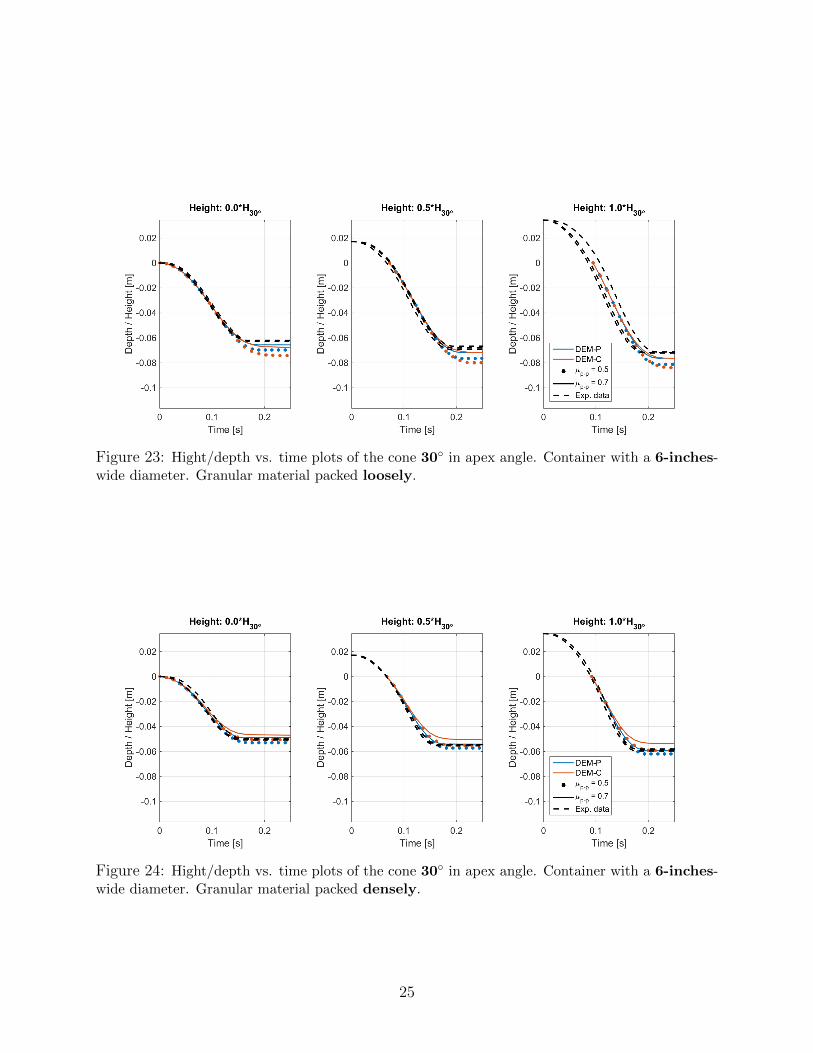
Figure 23: Hight/depth vs. time plots of the cone 30◦ in apex angle. Container with a 6-inches-wide diameter. Granular material packed loosely.
Figure 24: Hight/depth vs. time plots of the cone 30◦ in apex angle. Container with a 6-inches-wide diameter. Granular material packed densely.
25
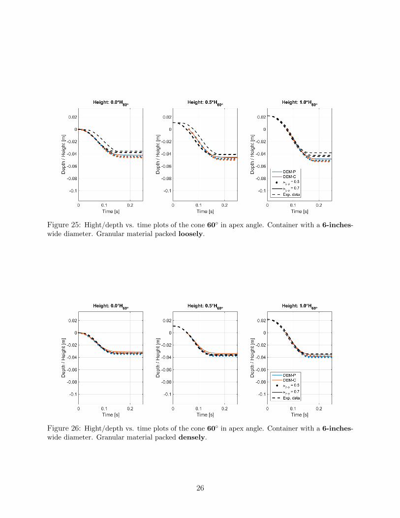
Figure 25: Hight/depth vs. time plots of the cone 60◦ in apex angle. Container with a 6-inches-wide diameter. Granular material packed loosely.
Figure 26: Hight/depth vs. time plots of the cone 60◦ in apex angle. Container with a 6-inches-wide diameter. Granular material packed densely.
26
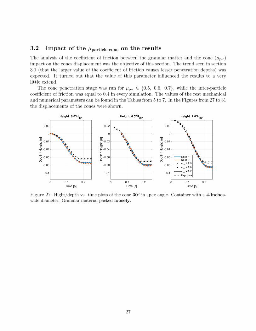
3.2 Impact of the µparticle-cone on the results
The analysis of the coefficient of friction between the granular matter and the cone (µp-c)impact on the cones displacement was the objective of this section. The trend seen in section3.1 (that the larger value of the coefficient of friction causes lesser penetration depths) wasexpected. It turned out that the value of this parameter influenced the results to a verylittle extend.
The cone penetration stage was run for µp-c ∈ {0.5, 0.6, 0.7}, while the inter-particlecoefficient of friction was equal to 0.4 in every simulation. The values of the rest mechanicaland numerical parameters can be found in the Tables from 5 to 7. In the Figures from 27 to 31the displacements of the cones were shown.
Figure 27: Hight/depth vs. time plots of the cone 30◦ in apex angle. Container with a 4-inches-wide diameter. Granular material packed loosely.
27

Figure 28: Hight/depth vs. time plots of the cone 30◦ in apex angle. Container with a 6-inches-wide diameter. Granular material packed loosely.
Figure 29: Hight/depth vs. time plots of the cone 30◦ in apex angle. Container with a 6-inches-wide diameter. Granular material packed densely.
28

Figure 30: Hight/depth vs. time plots of the cone 60◦ in apex angle. Container with a 6-inches-wide diameter. Granular material packed loosely.
Figure 31: Hight/depth vs. time plots of the cone 60◦ in apex angle. Container with a 6-inches-wide diameter. Granular material packed densely.
29

3.3 Granular material made of the “double-spheres”. The sensi-tivity analysis of the longitudinal dimension
The response of the mechanical system for the case where the granular material particleshad a shape of “double sphere” was also investigated. A double-sphere is defined as a bodythat consists of two spheres of equal diameters connected to each other. Its longitudinaldimension L is equal to md, where
m is a constant real number from the range [1.0, 2.0] and
d is a diameter of one of the spheres.
A cross-section of a double sphere with its dimensions was shown in the Figure 32. Acouple of examples of such particles for different values of m were shown in the Fig. 33.
Volume (V ), radii of gyration (kxx, kyy, kzz) and principal moments of inertia (Ixx, Iyy, Izz)of double sphere can be calculated from following equations:
V =
{4π3R3(1− cosϑ∗) if ϑ∗ ∈ [0, 90◦]
4π3R3(1 + cosϑ∗) if ϑ∗ ∈ [90◦, 180∗]
ixx = izz = 2%
2π
5R5(1− cosϑ∗)− π
5R5
[1
3(cos3 ϑ∗ − 1) + (1− cosϑ∗)
]+
2π
3(z′)2R3(1− cosϑ∗) +
π
2R4(z′)
√1− cos2 ϑ∗
if ϑ∗ ∈ [0, 90◦]
2π
5R5(1+ cosϑ∗)− π
5R5
[1
3(- cos3 ϑ∗ − 1) + (1+ cosϑ∗)
]+
2π
3(z′)2R3(1+ cosϑ∗) +
π
2R4(z′)
√1− cos2 ϑ∗
if ϑ∗ ∈ [90◦, 180◦]
iyy =
{4π5%R5
[13(+ cos3 ϑ∗ − 1) + (1− cosϑ∗)
]if ϑ∗ ∈ [0, 90◦]
4π5%R5
[13(- cos3 ϑ∗ − 1) + (1+ cosϑ∗)
]if ϑ∗ ∈ [90◦, 180◦]
k2xx = k2zz =ixxm
=ixxV %
k2yy =iyym
=iyyV %
Ixx = Izz = mk2xx Iyy = mk2yy
where:
V volume of double sphere
R radius of double sphere
z′ is equal to R− δ2
30

δ is the size of the overlap between two spheres
cosϑ∗ is equal to z′
R
% density
m mass
The y-direction was parallel to the longitudinal axis of the double sphere. Two remain-ing directions (x, z) were (obviously) perpendicular to y-axis. Results corresponding toϑ∗ ∈ [90◦, 180◦] are the ones describing double sphere (L = md > d). For the case where(L = md < d) the shape of the particle starts being similar to the lens; geometrical param-eters of a lens can be obtained from the formulas corresponding to ϑ∗ ∈ [0, 90◦]. Differencesbetween the equations describing lenses and double spheres were marked in red.
The sensitivity analysis of the longitudinal dimension impact on the depth at which thecone stopped penetrating the specimen was conducted on. The outcome of this analysis isshowed in the Fig. 35.
Figure 32: Dimensions of a double sphere. m ∈ [1.0, 2.0]
(a) m = 1.0 (b) m = 1.5 (c) m = 2.0
Figure 33: Cross-sections of double-spheres of different longitudinal dimension. In otherwords, double-spheres that have different values of parameter m.
31

Figure 34: ”Double-spheres” in 3D view
Figure 35: Depth at which the cone stopped penetrating the granular material as a function of thelongitudinal dimension of the double spheres. Plot shows the results obtained from the simulationsof cone having 30◦ in its apex angle; dropped from 34.36 mm above the specimen’s surface. Thegranular material had the inter-particle friction coefficient equal to 0.4 and µparticle-cone = 0.7.Container’s diameter was equal to 6 inches. Dashed lined show the depths reached by cones in thelaboratory tests.
32

4 Conclusion
1. Results from the simulations based on DEM-P and DEM-C approaches were compa-rable.
2. If calibrated correctly, both DEM-P and DEM-C can be used in simulating cone pen-etration test, giving the results close to the experimental ones.
3. DEM-C-based simulations were around 1.6 times slower than those based on DEM-P.
4. The simulations were sensitive to the value of the inter-particle coefficient of friction.
5. The value of the coefficient of friction between the particles and cone did not havethe major impact on the depths at which the cone stopped penetrating the granularmaterial.
6. If the grains were modeled as the double-spheres, the larger their longitudinal dimen-sion was, the smaller the penetration depths was.
33
References
[1] Fleischmann, J., 2015. DEM-PM Contact Model with Multi-Step Tangential ContactDisplacement History. Tech. Rep. TR-2015-06, Simulation-Based Engineering Labora-tory, University of Wisconsin-Madison.
[2] Negrut, D., and Serban, R., 2016. Posing Multibody Dynamics with Friction and Con-tact as a Differential Algebraic Inclusion Problem. Tech. Rep. TR-2016-12: http:
//sbel.wisc.edu/documents/TR-2016-12.pdf, Simulation-Based Engineering Labora-tory, University of Wisconsin-Madison.
[3] Project Chrono. Chrono: An Open Source Framework for the Physics-Based Simulationof Dynamic Systems. http://projectchrono.org. Accessed: 2016-03-07.
[4] Williams, K., 2016. Cone penetration results for 3mm glass beads and 20-30 Ottawasand. Tech. Rep. TR-2016-04: http://sbel.wisc.edu/documents/TR-2016-04.pdf,Simulation-Based Engineering Laboratory, University of Wisconsin-Madison.
[5] Elert, G. The Physics Factbook. Coefficients of Restitution, http://hypertextbook.com/facts/2006/restitution.shtml.
[6] The Engineering Toolbox. Friction and Friction Coefficients, http://www.
engineeringtoolbox.com/friction-coefficients-d_778.html.
[7] Kwarta, M., and Negrut, D., 2016. Using the Complementarity and Penalty Methods forSolving Frictional Contact Problems in Chrono: Validation for the Shear-Test with Par-ticle Image Velocimetry. Tech. Rep. TR-2016-18: http://sbel.wisc.edu/documents/
TR-2016-18.pdf, Simulation-Based Engineering Laboratory, University of Wisconsin-Madison.
[8] Kwarta, M., and Negrut, D., 2016. Using the Complementarity and Penalty Meth-ods for Solving Frictional Contact Problems in Chrono: Validation for the TriaxialTest. Tech. Rep. TR-2016-17: http://sbel.wisc.edu/documents/TR-2016-17.pdf,Simulation-Based Engineering Laboratory, University of Wisconsin-Madison.
34