technical support document for the proposed pm … support document for the proposed pm naaqs rule...

Technical Support Document for the Proposed PM NAAQS Rule

Response Surface Modeling

U.S. Environmental Protection Agency Office of Air Quality Planning and Standards

Research Triangle Park, NC 27711 February 2006

1

Table of Contents

I. Introduction ……….................................................................................................. 2 II. Emissions Inventories and Projections…………………………….......................... 2 III. Development of the Validation of Response Surface Modeling…………………... 7

A. Use of RSM …………………………….……………………………….… 8 B. Technical Approaches and Experimental Design of RSM .………….……. 9 B.1 CMAQ Modeling Platform for RSM ……………………………… 9 B.2 Statistical Technique used in RSM …………………………….…… 11 B.3 Modeling Scenarios and Emission Inventories and Sectors ….…... 13 B.4 Development of SMOKE/CMAQ Utility Interface Module ……..… 14 B.5 Selection of Emissions Control Factors and Control Ranges …...... 14

B.6 Selection of Regional vs. Local Impact ……………………........… 16 B.7 Output Metrics for CMAQ RSM PM2.5 ………………………….… 18 B.8 RSM Graphical Tool: Visual Policy Analyzer ……………........… 21 IV. Validation of Response Surface Modeling ………………………………….…….. 25

Appendix A: Control Scenario Model Runs Appendix B: Out-of-Sample Validation and Boundary Condition Runs

2

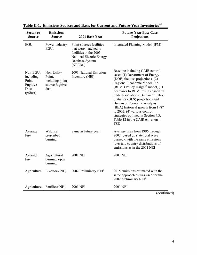
I. Introduction This Technical Support Document (TSD) describes the emissions inventories and air quality modeling performed by EPA for the development of the Response Surface Model (RSM) in support of the Regulatory Impact Assessment (RIA) for the proposed National Ambient Air Quality Standards (NAAQS) for PM2.5. Included is information on (1) the emissions inventories and development of projections, (2) the air quality modeling and development of model inputs, (3) development and experimental design of the RSM, and (4) the performance and validation of the RSM as compared to the air quality modeling. The RSM is based on a new approach known as air quality metamodeling that aggregates numerous pre-specified individual air quality modeling simulations into a multi-dimensional air quality “response surface”. Simply, this metamodeling technique is a “model of the model” and can be shown to reproduce the results from an individual modeling simulation with little bias or error. The RSM incorporates statistical relationships between model inputs and outputs to provide real-time estimate of these air quality changes. The RSM provides a wide breadth of model outputs, which we utilize to develop emissions control scenarios. The RSM approach informs the selection and evaluation of various control scenarios. This approach allows for the rapid assessment of air quality impacts of different combinations of emissions reductions and was used to estimate air quality changes for various control scenarios for the proposed PM2.5 NAAQS. II. Emissions Inventories and Projections Emission inventories were developed for the 48 contiguous States, the District of Columbia, and portions of Canada and Mexico for the purposes of modeling particulate matter (PM) to support the air quality modeling analyses for the RSM development and the proposed PM NAAQS. The model required hourly emissions for the entire year of 2001 and future years on a 36-km national grid of the following pollutants: carbon monoxide (CO), nitrogen oxides (NOX), volatile organic compounds (VOC), sulfur dioxide (SO2), ammonia (NH3), particulate matter less than or equal to 10 microns (PM10), and particulate matter less than or equal to 2.5 microns (PM2.5). The emission sources and the basis for current and future-year emission inventories for the Clean Air Interstate Rule (CAIR), and the PM NAAQS proposal are listed in Table II-1. Readers interested in additional technical detail describing how EPA developed and projected this inventory to 2010 and 2015 can reference the CAIR Emissions Inventory TSD.1 Section 3 in the CAIR TSD details the 2001 baseline emissions used in each of the inventory sectors in Table II-1. Section 4 in the CAIR TSD details the growth and control methodology used in the 2010 and 2015 CAIR control strategy inventories.

1 See: http://www.epa.gov/interstateairquality/pdfs/finaltech01.pdf. Additional information may be found in Appendix H of the Clean Air Interstate Rule Emissions Inventory TSD, March 2005.

3

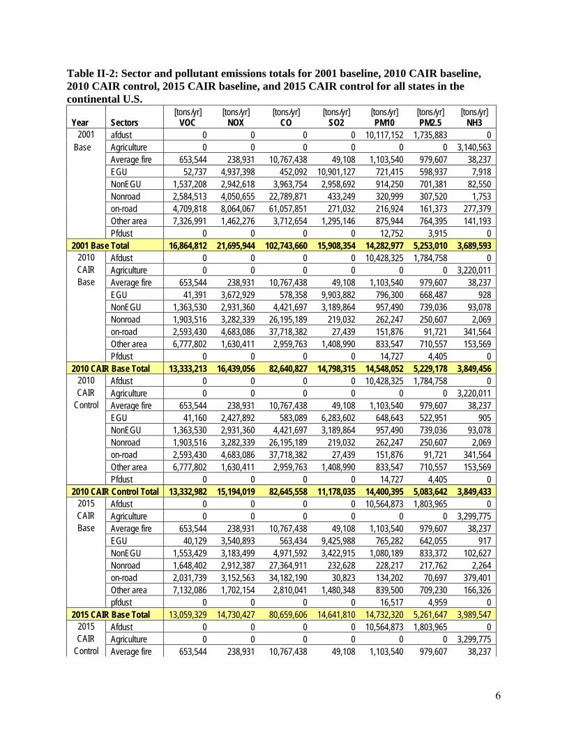
Table II-2 provides summaries for 2001, 2010 CAIR baseline and control, and 2015 CAIR baseline and control emissions by pollutant and inventory sector, as defined in Table II-1, for states in the continental U.S. Appendix B and Appendix H in the CAIR TSD include more detailed summaries that expand the 2001 baseline and 2015 CAIR control strategy (respectively) emissions in Table II-2 to include totals by state, sector and pollutant. Except for the future CAIR control strategy EGU emissions; this information is also available electronically in the CAIR docket (item number OAR-2003-0053-1705) and the CAIR website: http://www.epa.gov/cleanairinterstaterule/technical.html , as a Microsoft®

Excel® file, named

Emissions_summary_state_sector_2001-2010-2015.xls. Also available are annual total emissions by state and sector (except for CAIR control strategy EGU emissions) after application of chemical speciation factors for 2001, 2010, and 2015, which includes differences among the years. It can be found as a Microsoft®

Excel® file

Emissions_summary_state_sector_speciation_2001-2010-2015.xls in the CAIR docket (item number OAR-2003-0053-1706) and the CAIR website.

4

Table II-1. Emissions Sources and Basis for Current and Future-Year Inventoriesa,b

Sector or Source

Emissions Source 2001 Base Year

Future-Year Base Case Projections

EGU Power industry EGUs

Point-sources facilities that were matched to facilities in the 2003 National Electric Energy Database System (NEEDS)

Integrated Planning Model (IPM)

Non-EGU, including Point Fugitive Dust (pfdust)

Non-Utility Point, including point source fugitive dust

2001 National Emission Inventory (NEI)

Baseline including CAIR control case: (1) Department of Energy (DOE) fuel use projections, (2) Regional Economic Model, Inc. (REMI) Policy Insight® model, (3) decreases to REMI results based on trade associations, Bureau of Labor Statistics (BLS) projections and Bureau of Economic Analysis (BEA) historical growth from 1987 to 2002, (4) various control strategies outlined in Section 4.3, Table 12 in the CAIR emissions TSD

Average Fire

Wildfire, prescribed burning

Same as future year Average fires from 1996 through 2002 (based on state total acres burned), with the same emissions rates and country distributions of emissions as in the 2001 NEI

Average Fire

Agricultural burning, open burning

2001 NEI 2001 NEI

Agriculture Livestock NH3 2002 Preliminary NEIc 2015 emissions estimated with the same approach as was used for the 2002 preliminary NEIc

Agriculture Fertilizer NH3 2001 NEI 2001 NEI

(continued)

5

Table II-1. Emissions Sources and Basis for Current and Future-Year Inventoriesa,b (continued)

Sector or Source

Emissions Source 2001 Base Year

Future-Year Base Case Projections

Other Area, including Area Fugitive Dust (afdust)

All other stationary area sources, including area-source fugitive dust

1999 NEI, version 3 grown to 2001

(1) DOE fuel use projections, (2) REMI Policy Insight Model, (3) decreases to REMI results based on trade associations, BLS projections and BEA historical growth from 1987 – 2002, (4) various control strategies outlined in Section 4.3, Table 13 in the CAIR emissions TSD

On-road Highway vehicles

Except for California, the National Mobile Inventory Model (NMIM) using the Mobile6.2 model. California used their won on-road mobile source estimation model (EMFAC2002), which were assigned pollutant-specific monthly variation from NMIM.

Except for California, projected vehicle miles traveled same as CAIR proposed and final rule, emissions from MOBILE6.2 model. For California, 2001 emissions were grown by county and SCC using NMIM 2001 to future year ratios.

Nonroad Locomotives, commercial marine vessels, and aircraft

2001 NEI; CMV adjusted to new national totals from Office of Transportation Air Quality (OTAQ)

Grown based on national totals from OTAQ, using state/county distribution of emissions from the 2001 NEI

Nonroad All other nonroad vehicles

NONROAD 2004 model NONROAD 2004 model

a This table documents only the sources of data for the U.S. inventory. The sources of data used for Canada and

Mexico are explained in the CAIR emissions inventory technical support document. b All fugitive dust emissions were adjusted downward using county-specific transportable fractions needed as

part of the current state of the art in air quality modeling. c ftp://ftp.epa.gov/EmisInventory/prelim2002nei/nonpoint/documentation/nh3inventorydraft_jan2004.pdf.

6

Table II-2: Sector and pollutant emissions totals for 2001 baseline, 2010 CAIR baseline, 2010 CAIR control, 2015 CAIR baseline, and 2015 CAIR control for all states in the continental U.S.

Year Sectors [tons/yr]

VOC [tons/yr]

NOX [tons/yr]

CO [tons/yr]

SO2 [tons/yr] PM10

[tons/yr] PM2.5

[tons/yr]NH3

2001 afdust 0 0 0 0 10,117,152 1,735,883 0 Base Agriculture 0 0 0 0 0 0 3,140,563 Average fire 653,544 238,931 10,767,438 49,108 1,103,540 979,607 38,237 EGU 52,737 4,937,398 452,092 10,901,127 721,415 598,937 7,918 NonEGU 1,537,208 2,942,618 3,963,754 2,958,692 914,250 701,381 82,550 Nonroad 2,584,513 4,050,655 22,789,871 433,249 320,999 307,520 1,753 on-road 4,709,818 8,064,067 61,057,851 271,032 216,924 161,373 277,379 Other area 7,326,991 1,462,276 3,712,654 1,295,146 875,944 764,395 141,193 Pfdust 0 0 0 0 12,752 3,915 0 2001 Base Total 16,864,812 21,695,944 102,743,660 15,908,354 14,282,977 5,253,010 3,689,593

2010 Afdust 0 0 0 0 10,428,325 1,784,758 0 CAIR Agriculture 0 0 0 0 0 0 3,220,011 Base Average fire 653,544 238,931 10,767,438 49,108 1,103,540 979,607 38,237

EGU 41,391 3,672,929 578,358 9,903,882 796,300 668,487 928 NonEGU 1,363,530 2,931,360 4,421,697 3,189,864 957,490 739,036 93,078 Nonroad 1,903,516 3,282,339 26,195,189 219,032 262,247 250,607 2,069 on-road 2,593,430 4,683,086 37,718,382 27,439 151,876 91,721 341,564 Other area 6,777,802 1,630,411 2,959,763 1,408,990 833,547 710,557 153,569 Pfdust 0 0 0 0 14,727 4,405 0

2010 CAIR Base Total 13,333,213 16,439,056 82,640,827 14,798,315 14,548,052 5,229,178 3,849,456 2010 Afdust 0 0 0 0 10,428,325 1,784,758 0 CAIR Agriculture 0 0 0 0 0 0 3,220,011

Control Average fire 653,544 238,931 10,767,438 49,108 1,103,540 979,607 38,237 EGU 41,160 2,427,892 583,089 6,283,602 648,643 522,951 905 NonEGU 1,363,530 2,931,360 4,421,697 3,189,864 957,490 739,036 93,078 Nonroad 1,903,516 3,282,339 26,195,189 219,032 262,247 250,607 2,069 on-road 2,593,430 4,683,086 37,718,382 27,439 151,876 91,721 341,564 Other area 6,777,802 1,630,411 2,959,763 1,408,990 833,547 710,557 153,569 Pfdust 0 0 0 0 14,727 4,405 0 2010 CAIR Control Total 13,332,982 15,194,019 82,645,558 11,178,035 14,400,395 5,083,642 3,849,433

2015 Afdust 0 0 0 0 10,564,873 1,803,965 0 CAIR Agriculture 0 0 0 0 0 0 3,299,775 Base Average fire 653,544 238,931 10,767,438 49,108 1,103,540 979,607 38,237

EGU 40,129 3,540,893 563,434 9,425,988 765,282 642,055 917 NonEGU 1,553,429 3,183,499 4,971,592 3,422,915 1,080,189 833,372 102,627 Nonroad 1,648,402 2,912,387 27,364,911 232,628 228,217 217,762 2,264 on-road 2,031,739 3,152,563 34,182,190 30,823 134,202 70,697 379,401 Other area 7,132,086 1,702,154 2,810,041 1,480,348 839,500 709,230 166,326 pfdust 0 0 0 0 16,517 4,959 0 2015 CAIR Base Total 13,059,329 14,730,427 80,659,606 14,641,810 14,732,320 5,261,647 3,989,547

2015 Afdust 0 0 0 0 10,564,873 1,803,965 0 CAIR Agriculture 0 0 0 0 0 0 3,299,775

Control Average fire 653,544 238,931 10,767,438 49,108 1,103,540 979,607 38,237

7

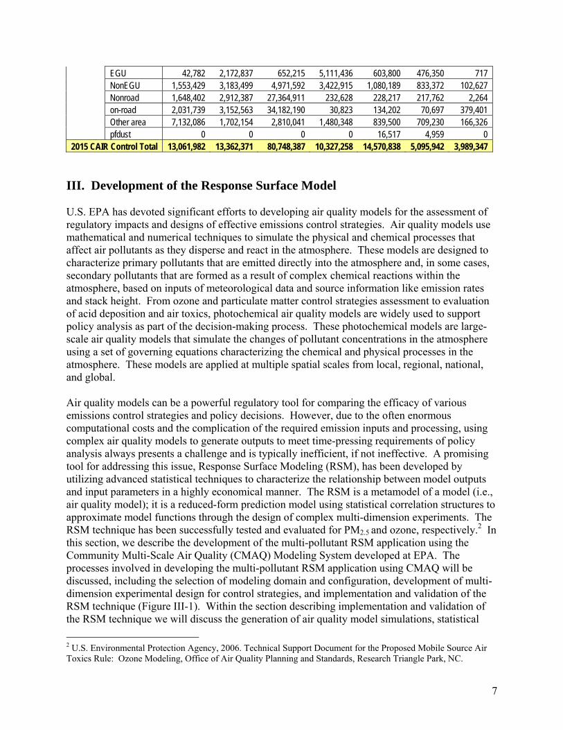
EGU 42,782 2,172,837 652,215 5,111,436 603,800 476,350 717 NonEGU 1,553,429 3,183,499 4,971,592 3,422,915 1,080,189 833,372 102,627 Nonroad 1,648,402 2,912,387 27,364,911 232,628 228,217 217,762 2,264 on-road 2,031,739 3,152,563 34,182,190 30,823 134,202 70,697 379,401 Other area 7,132,086 1,702,154 2,810,041 1,480,348 839,500 709,230 166,326 pfdust 0 0 0 0 16,517 4,959 0 2015 CAIR Control Total 13,061,982 13,362,371 80,748,387 10,327,258 14,570,838 5,095,942 3,989,347

III. Development of the Response Surface Model U.S. EPA has devoted significant efforts to developing air quality models for the assessment of regulatory impacts and designs of effective emissions control strategies. Air quality models use mathematical and numerical techniques to simulate the physical and chemical processes that affect air pollutants as they disperse and react in the atmosphere. These models are designed to characterize primary pollutants that are emitted directly into the atmosphere and, in some cases, secondary pollutants that are formed as a result of complex chemical reactions within the atmosphere, based on inputs of meteorological data and source information like emission rates and stack height. From ozone and particulate matter control strategies assessment to evaluation of acid deposition and air toxics, photochemical air quality models are widely used to support policy analysis as part of the decision-making process. These photochemical models are large-scale air quality models that simulate the changes of pollutant concentrations in the atmosphere using a set of governing equations characterizing the chemical and physical processes in the atmosphere. These models are applied at multiple spatial scales from local, regional, national, and global. Air quality models can be a powerful regulatory tool for comparing the efficacy of various emissions control strategies and policy decisions. However, due to the often enormous computational costs and the complication of the required emission inputs and processing, using complex air quality models to generate outputs to meet time-pressing requirements of policy analysis always presents a challenge and is typically inefficient, if not ineffective. A promising tool for addressing this issue, Response Surface Modeling (RSM), has been developed by utilizing advanced statistical techniques to characterize the relationship between model outputs and input parameters in a highly economical manner. The RSM is a metamodel of a model (i.e., air quality model); it is a reduced-form prediction model using statistical correlation structures to approximate model functions through the design of complex multi-dimension experiments. The RSM technique has been successfully tested and evaluated for PM2.5 and ozone, respectively.2 In this section, we describe the development of the multi-pollutant RSM application using the Community Multi-Scale Air Quality (CMAQ) Modeling System developed at EPA. The processes involved in developing the multi-pollutant RSM application using CMAQ will be discussed, including the selection of modeling domain and configuration, development of multi-dimension experimental design for control strategies, and implementation and validation of the RSM technique (Figure III-1). Within the section describing implementation and validation of the RSM technique we will discuss the generation of air quality model simulations, statistical 2 U.S. Environmental Protection Agency, 2006. Technical Support Document for the Proposed Mobile Source Air Toxics Rule: Ozone Modeling, Office of Air Quality Planning and Standards, Research Triangle Park, NC.

8

modeling and construction of representative surfaces, model validation, and development of the Visual Policy Analyzer, a standalone software tool for viewing and manipulating the response surface.

Figure III-1. Flow diagram identifying key steps within the development of Response Surface Modeling. A. Use of RSM The RSM is intended to provide a modeling surrogate tool that can effectively simulate real-time PM impacts for a variety of regulatory alternatives for use in Regulatory Impact Analyses. For

9

example, generating estimates of the health benefits of reductions in PM precursors and providing screening level estimates of the impacts of control strategies on NAAQS design values are functions the RSM supports. While the RSM may not provide a complete picture of all changes necessary to reach various alternative standards nationwide, it is highly useful in the context of providing illustrative control scenarios for selected areas, and understanding the contribution of different source categories, source regions and pollutant emissions to air quality across the U.S. The RSM can be used in a variety of ways: (1) strategy design and assessment (e.g. comparison of urban vs. regional controls; comparison across sectors; comparison across pollutants); (2) optimization (develop optimal combinations of controls to attain standards at minimum cost); (3) model sensitivity (systematically evaluate the relative sensitivity of modeled ozone and PM levels to changes in emissions inputs. B. Technical Approaches and Experimental Design of RSM B.1 CMAQ Modeling Platform for RSM Multi-pollutant (particulate matter (PM2.5) and ozone) air quality modeling was performed using the Community Multi-scale Air Quality (CMAQ) model for the development of an integrated PM2.5 and ozone Response Surface Model (RSM). Precursors of both PM2.5 and ozone and their transformations and transport were modeled. For the purpose of the PM2.5 NAAQS RIA, model evaluation and control strategy assessment will focus exclusively on PM2.5, its constituents and precursors. Currently, the RSM is used as the foundation to conceptualize control strategy scenarios and resulting outcomes. Likewise, the use of RSM will be extended to investigate and better inform sector based control scenarios based on a multi-pollutant approach (i.e., ozone and PM analyses). CMAQ is a three-dimensional regional grid-based air quality model designed to simulate particulate matter and ozone concentrations and deposition over large spatial scales (e.g., over the contiguous U.S.) over an extended period of time (e.g., up to a year).3 The CMAQ model includes state-of-the-science capabilities for conducting urban to regional scale simulations of multiple air quality issues, including tropospheric ozone, fine particles, toxics, acid deposition, and visibility degradation. The CMAQ model is a publicly available (supported by the Community Modeling and Analysis System (CMAS) Center; http://www.cmascenter.org/), peer reviewed, state-of-the-science model consisting of a number of science attributes that are critical for simulating the oxidant precursors and non-linear organic and inorganic chemical relationships associated with the formation of sulfate, nitrate, and organic aerosols. CMAQ also

3 Dennis, R.L., Byun, D.W., Novak, J.H., Galluppi, K.J., Coats, C.J., and Vouk, M.A., 1996. The next generation of integrated air quality modeling: EPA’s Models-3, Atmospheric Environment, 30, 1925-1938. Byun, D.W., and Ching, J.K.S., Eds, 1999. Science algorithms of EPA Models-3 Community Multiscale Air Quality (CMAQ modeling system, EPA/600/R-99/030, Office of Research and Development, U.S. Environmental Protection Agency. Byun, D.W., and Schere, K.L., 2006. Review of the Governing Equations, Computational Algorithms, and Other Components of the Models-3 community Multiscale Air Quality (CMAQ) Modeling System. J. Applied Mechanics Reviews, Accepted.

10

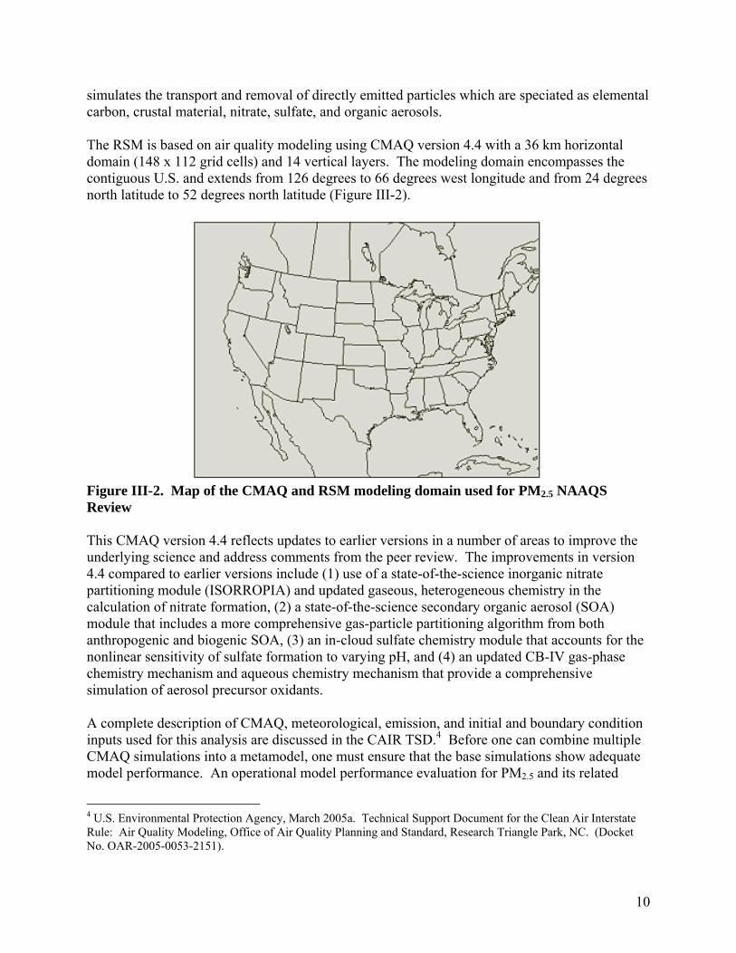
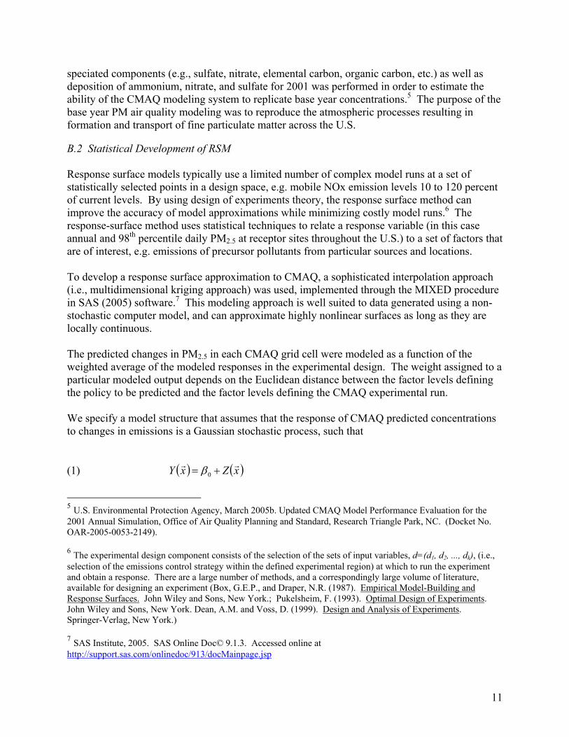
simulates the transport and removal of directly emitted particles which are speciated as elemental carbon, crustal material, nitrate, sulfate, and organic aerosols. The RSM is based on air quality modeling using CMAQ version 4.4 with a 36 km horizontal domain (148 x 112 grid cells) and 14 vertical layers. The modeling domain encompasses the contiguous U.S. and extends from 126 degrees to 66 degrees west longitude and from 24 degrees north latitude to 52 degrees north latitude (Figure III-2).

Figure III-2. Map of the CMAQ and RSM modeling domain used for PM2.5 NAAQS Review This CMAQ version 4.4 reflects updates to earlier versions in a number of areas to improve the underlying science and address comments from the peer review. The improvements in version 4.4 compared to earlier versions include (1) use of a state-of-the-science inorganic nitrate partitioning module (ISORROPIA) and updated gaseous, heterogeneous chemistry in the calculation of nitrate formation, (2) a state-of-the-science secondary organic aerosol (SOA) module that includes a more comprehensive gas-particle partitioning algorithm from both anthropogenic and biogenic SOA, (3) an in-cloud sulfate chemistry module that accounts for the nonlinear sensitivity of sulfate formation to varying pH, and (4) an updated CB-IV gas-phase chemistry mechanism and aqueous chemistry mechanism that provide a comprehensive simulation of aerosol precursor oxidants. A complete description of CMAQ, meteorological, emission, and initial and boundary condition inputs used for this analysis are discussed in the CAIR TSD.4 Before one can combine multiple CMAQ simulations into a metamodel, one must ensure that the base simulations show adequate model performance. An operational model performance evaluation for PM2.5 and its related

4 U.S. Environmental Protection Agency, March 2005a. Technical Support Document for the Clean Air Interstate Rule: Air Quality Modeling, Office of Air Quality Planning and Standard, Research Triangle Park, NC. (Docket No. OAR-2005-0053-2151).

11

speciated components (e.g., sulfate, nitrate, elemental carbon, organic carbon, etc.) as well as deposition of ammonium, nitrate, and sulfate for 2001 was performed in order to estimate the ability of the CMAQ modeling system to replicate base year concentrations.5 The purpose of the base year PM air quality modeling was to reproduce the atmospheric processes resulting in formation and transport of fine particulate matter across the U.S. B.2 Statistical Development of RSM Response surface models typically use a limited number of complex model runs at a set of statistically selected points in a design space, e.g. mobile NOx emission levels 10 to 120 percent of current levels. By using design of experiments theory, the response surface method can improve the accuracy of model approximations while minimizing costly model runs.6 The response-surface method uses statistical techniques to relate a response variable (in this case annual and 98th percentile daily PM2.5 at receptor sites throughout the U.S.) to a set of factors that are of interest, e.g. emissions of precursor pollutants from particular sources and locations. To develop a response surface approximation to CMAQ, a sophisticated interpolation approach (i.e., multidimensional kriging approach) was used, implemented through the MIXED procedure in SAS (2005) software.7 This modeling approach is well suited to data generated using a non-stochastic computer model, and can approximate highly nonlinear surfaces as long as they are locally continuous. The predicted changes in PM2.5 in each CMAQ grid cell were modeled as a function of the weighted average of the modeled responses in the experimental design. The weight assigned to a particular modeled output depends on the Euclidean distance between the factor levels defining the policy to be predicted and the factor levels defining the CMAQ experimental run. We specify a model structure that assumes that the response of CMAQ predicted concentrations to changes in emissions is a Gaussian stochastic process, such that (1) ( ) ( )xZxY rr

+= 0β

5 U.S. Environmental Protection Agency, March 2005b. Updated CMAQ Model Performance Evaluation for the 2001 Annual Simulation, Office of Air Quality Planning and Standard, Research Triangle Park, NC. (Docket No. OAR-2005-0053-2149). 6 The experimental design component consists of the selection of the sets of input variables, d=(d1, d2, ..., dk), (i.e., selection of the emissions control strategy within the defined experimental region) at which to run the experiment and obtain a response. There are a large number of methods, and a correspondingly large volume of literature, available for designing an experiment (Box, G.E.P., and Draper, N.R. (1987). Empirical Model-Building and Response Surfaces. John Wiley and Sons, New York.; Pukelsheim, F. (1993). Optimal Design of Experiments. John Wiley and Sons, New York. Dean, A.M. and Voss, D. (1999). Design and Analysis of Experiments. Springer-Verlag, New York.) 7 SAS Institute, 2005. SAS Online Doc© 9.1.3. Accessed online at http://support.sas.com/onlinedoc/913/docMainpage.jsp

12

where Y is the species output metric, xr is the vector of emissions factors (defined between 0 and 1.2), 0β is the mean response (estimated), and ( )xZ r is a Gaussian process assumed to have mean 0, variance σ2, and a correlation structure defined by (2) ( ) ( )( )( )( )222 ,exp, θσ jiji xxdistxxR rrrr

−= where ixr is the vector of factor values associated with run i of the experimental design,

( )ji xxdist rr ,2 is the squared distance between the vectors of factors associated with runs i and j, and θ and σ2 are parameters to be estimated. The variance (σ2) and correlation (θ) parameters are fit using maximum likelihood methods. Based on the estimated parameters and the available CMAQ model results, the predicted value for a given species metric is obtained using the equation (3) ( ) ( ) ( )0

1000

ˆˆˆ ββ −+= − yRxrxy t rrr where 0xr is the vector of factor values for which we want a predicted species response, ( )0ˆ xy r is

the prediction at 0xr , 0β̂ is the estimate of 0β , R is the matrix of all design points correlated with

each other based on equation (2) (with θ̂ as the estimate of θ), R-1 is the inverse of R, ( )0xrt r is the transpose of the vector or correlations, between 0xr and each of the design points, namely,

( ) ( ) ( )( )Tnt xxRxxRxr rrrrr ,,...,, 0100 = , and yr is the vector of the particular species response metrics

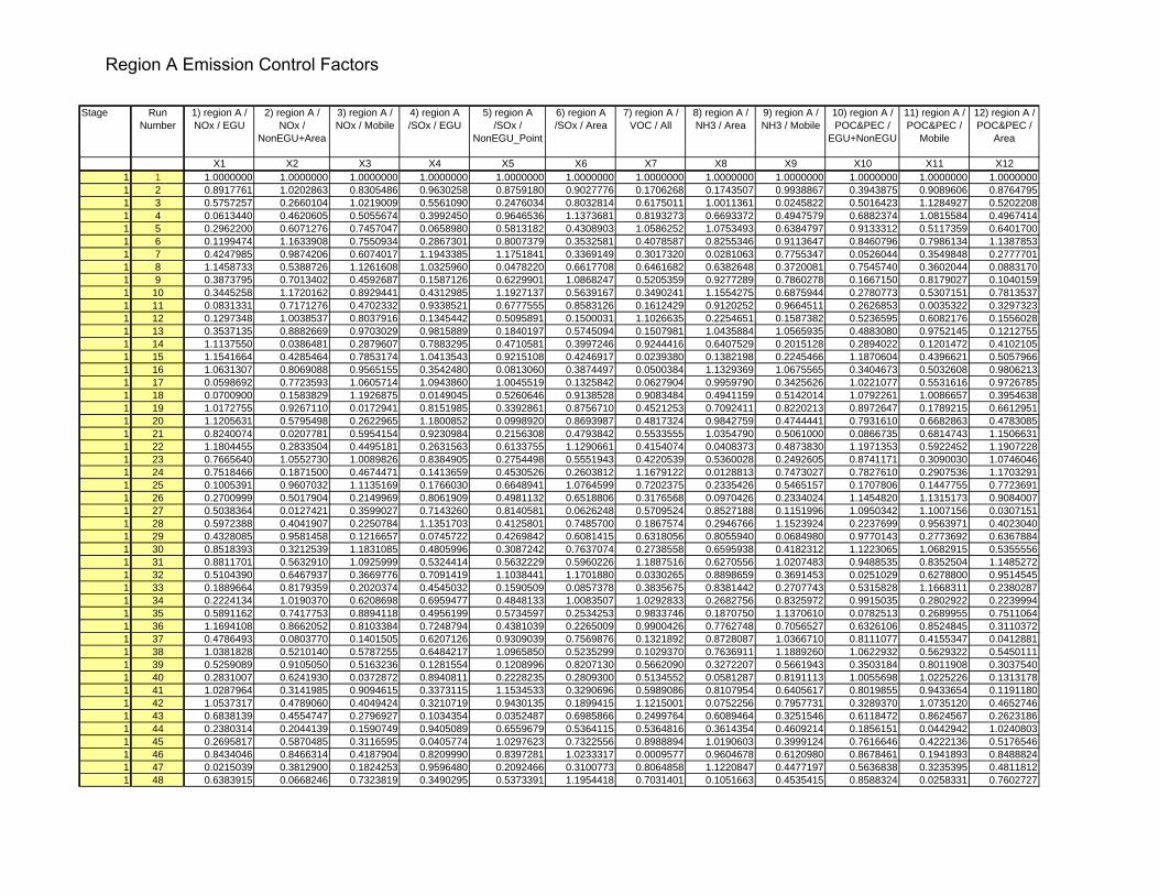
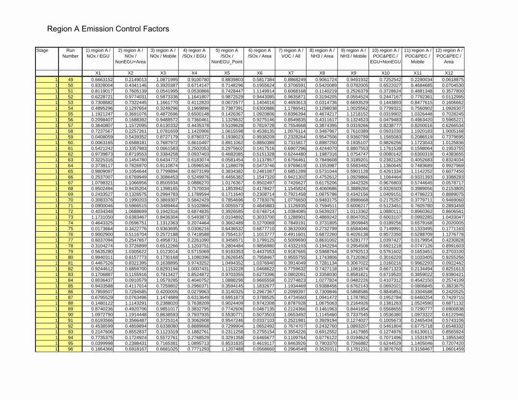
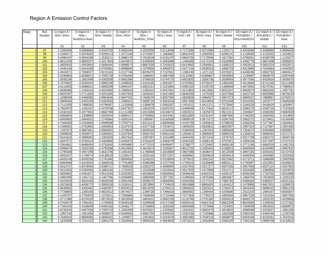
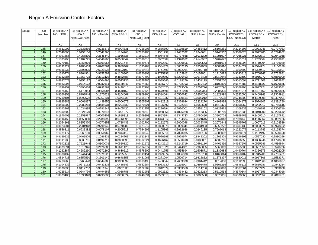
associated with the design points. In this specific application, the design points are the 180 xr vectors, each of length 12, consisting of the selected 12 emission control factors defined below in Section B.5. The vector 0xr consists of the values of the 12 factors for which the predicted species metric is desired. yr is the vector of CMAQ modeled species metric values and has 180 elements. The matrix R is formed as a 180x180 matrix with a row and column for each design point. The value in each cell of R is determined by equation (2). The RSM experimental design covers a change in the baseline emissions of zero to 120 percent, utilizing a staged Latin Hypercube statistical method. This statistical method follows a space filling design within the policy area and policy controls in order to accurately capture the linear and nonlinear interactions among pollutants. The Latin hypercube design retains flexibility, which accommodates the number of runs selected based on limitations (computer resources). A total of 180 CMAQ model runs were conducted (a base case run plus 179 control runs). The model runs were broken into two stages, 120 runs in the first stage and 60 runs each in stage two. This allowed for faster development of preliminary surfaces and allowed testing of additional predictive power for additional model runs. The set of CMAQ simulations provide inputs to the statistical response surface modeling. The complete list of model runs and corresponding control scenarios (selection of policy factor controls) are provided in Appendix A. The CMAQ model

13

was applied for the 2010 CAIR projection baseline in order to provide annual PM2.5 concentrations, visibility, and deposition estimates. The CMAQ model was run for 4 months, one month from each season, February, April, July, October, in order to reduce computational time for such a large number of annual model runs. These months were chosen based on greatest predictability of the quarterly mean. Each quarterly run included a 5-day ramp-up (i.e., "spin-up") period designed to minimize the influence of the initial concentration fields (i.e., initial conditions) used at the start of the model run. The development of initial condition concentrations is described in the CAIR TSD. The ramp-up periods used for the RSM CMAQ applications are as follows:

- First quarter ramp-up period is January 27 - 31, 2001 - Second quarter ramp-up period is March 27 - 31, 2001 - Third quarter ramp-up period is June 26 - 30, 2001 - Fourth quarter ramp-up period is September 26 - 30, 2001

Model predictions from these ramp-up periods were discarded and not used in analyses of the modeling results. Once the response surface model has been generated, it can be used to simulate the functions of the more computationally expensive atmospheric chemistry model. The RSM can be used to derive analytical representations of model sensitivities to changes in model inputs. For example, the RSM is designed to show how CMAQ (air quality model) predicts the atmosphere would respond to emission reductions for selected sources and pollutants, though it does not provide how those reductions in pollutants can be accomplished (i.e. specific control technologies). The RSM allows for comparison on an equal footing of controls for different source/pollutant combinations, and between local and regional sources. It should be noted that because RSM is built from CMAQ air quality model runs, it therefore has the same strengths and limitations of the underlying model and its inputs. B.3 Modeling Scenarios and Emission Inventories and Sectors The PM NAAQS RIA modeled relative changes in air quality for the entire U.S. using the Response Surface Model (RSM) applied to the 2010 regulatory Base Case developed by EPA as part of the analysis for the Clean Air Interstate Rule (CAIR). While CAIR targets controls of SO2 and NOx in the Eastern United States, the other rules/programs in the 2010 baseline include Clean Air Non-Road Diesel Rule, Heavy Duty Diesel Rule, Tier 2, and the NOx SIP Call. Because our base year of analysis is 2015, we extrapolate the baseline year from 2010 to 2015 and to include CAIR controls.8 2015 serves as a logical base year for analysis because it is a reasonable estimate of the date by which States would begin to implement controls to attain the revised standard; assuming promulgation in 2006, designations would require 3 years, and States would then have 5 years to attain. The RSM control strategy outputs are based on projected

8 We developed the RSM with a 2010 baseline so that it could serve the analytical needs of both the final PM NAAQS implementation rule (due in late 2006) for the current standard as well as the PM NAAQS RIA for the revised standard.

14

2015 post-CAIR emissions inventories and therefore reflect any uncertainties in those inventories. Certain source/pollutant inventories may be more uncertain than others. B.4 Development of SMOKE/CMAQ Utility Interface Module A pre-requisite task of the integrated PM2.5 and ozone CMAQ RSM effort was to develop an interface utility module within the CMAQ to allow the model to directly read the pre-merged SMOKE emission files (e.g., 3-D point sources, 2-D mobile sources, 2-D area sources, 2-D biogenic, sources, etc.), and more importantly, allow the model to directly control the % emission reduction/increase for the RSM scenarios runs that are needed for constructing the PM2.5 and O3 response surfaces. This tool increased the capacity and functionality of the operational CMAQ RSM models runs while (1) eliminating massive emission inputs for CMAQ RSM modeling (2) leading to highly efficient RSM modeling since the process can be automated to eliminate tedious manual operations. A SMOKE/CMAQ interface module has been developed as part of CMAQ system to facilitate and expedite these CMAQ RSM simulations. B.5 Selection of Emissions Control Factors and Control Ranges The main purpose of the RSM is to demonstrate the impact of various reductions in precursor emissions from different combinations of sources on air quality. Therefore, constraints were placed on the experimental design space, i.e. the region over which the response is studied, to a set of variables that parameterize a set of possible emissions control strategies, and evaluate the change in ambient PM2.5 levels that result from a change (reduction or increase) in emissions.9 Selection of policy factors were based on precursor emission type and source category relevant to policy analysis of interest. The experimental design carefully considered factors that would provide maximum information for use in comparing relative efficacy of different emissions control strategies. Hence, 12 variable emission control factors were selected based on precursor emission type and source category, as well as balancing computational efficiency of model runs and resources available. The selection of factors was based on three fundamental areas:

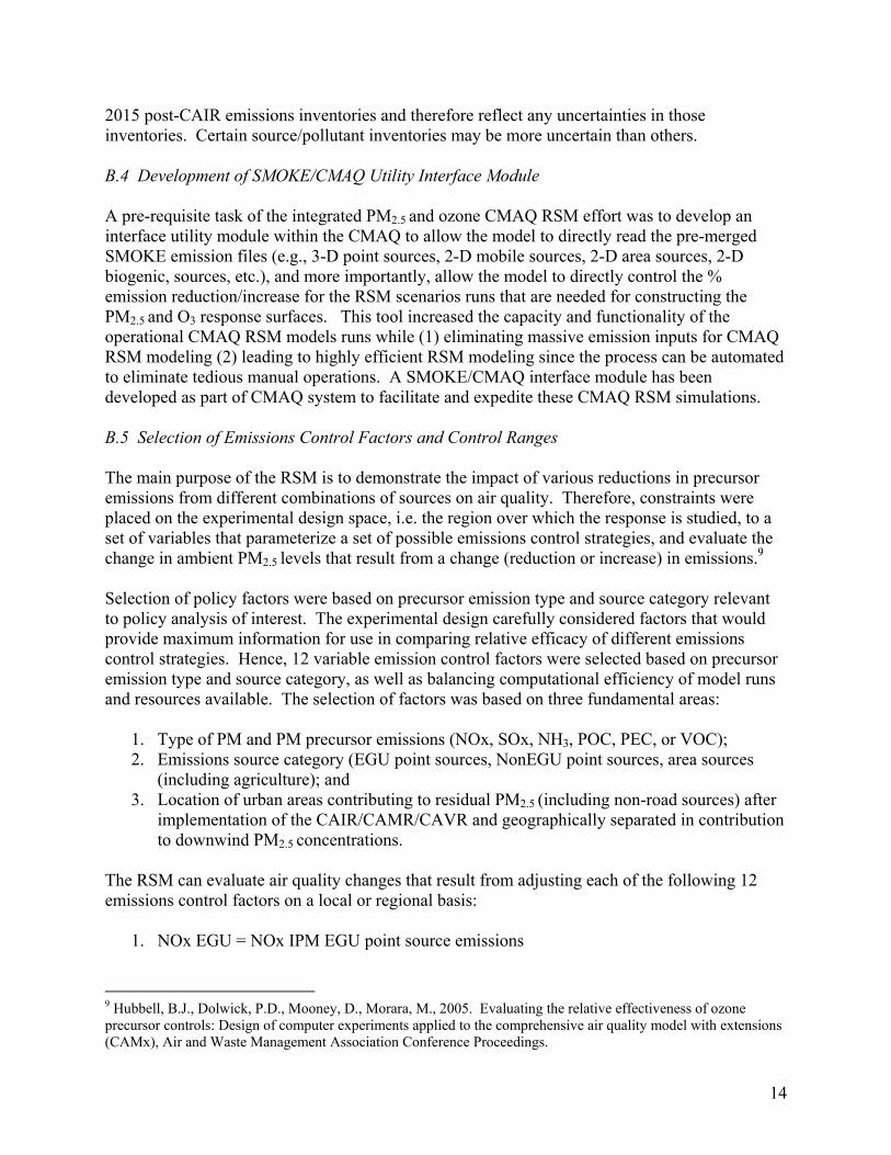
1. Type of PM and PM precursor emissions (NOx, SOx, NH3, POC, PEC, or VOC); 2. Emissions source category (EGU point sources, NonEGU point sources, area sources

(including agriculture); and 3. Location of urban areas contributing to residual PM2.5 (including non-road sources) after

implementation of the CAIR/CAMR/CAVR and geographically separated in contribution to downwind PM2.5 concentrations.

The RSM can evaluate air quality changes that result from adjusting each of the following 12 emissions control factors on a local or regional basis:

1. NOx EGU = NOx IPM EGU point source emissions

9 Hubbell, B.J., Dolwick, P.D., Mooney, D., Morara, M., 2005. Evaluating the relative effectiveness of ozone precursor controls: Design of computer experiments applied to the comprehensive air quality model with extensions (CAMx), Air and Waste Management Association Conference Proceedings.

15

2. NOx NonEGU Point and Area = NOx IPM Non-EGU point source, area source, and agricultural source emissions

3. NOx Mobile = NOx nonroad source and mobile source emissions 4. SOx EGU = SOx IPM EGU point source emissions 5. SOx NonEGU Point = SOx IPM Non-EGU point source emissions 6. SOx Area = SOx area source and agricultural source emissions 7. NH3 Area = Ammonia area source and agricultural source emissions 8. NH3 Mobile = Ammonia non-road source and mobile source sources 9. POC/PEC Point (EGU and NonEGU) = Elemental carbon and organic carbon IPM EGU

point source and IPM Non-EGU point source emissions 10. POC/PEC Mobile = Elemental carbon and organic carbon nonroad source and mobile

source emissions 11. POC/PEC Area = Elemental carbon and organic carbon area source and agricultural

source emissions 12. VOC All = Volatile organic carbon IPM EGU point source, IPM Non-EGU point source,

area source, agricultural source, nonroad source, and mobile source emissions10 Source groupings with small contributions to emissions were grouped with similar larger source groupings for efficiency (Figure III-3). NonEGU Area NOx and SOx sources were primarily smaller industrial combustion sources, such as coal, oil, and natural gas powered boilers and internal combustion engines. Agricultural area sources were only significant contributors to ammonia emissions. VOC sources were lumped together because VOCs are not expected to influence PM levels significantly.

Figure III-3. National analysis of source contributions to emissions sectors.11

10 This version of the RSM did not address direct emissions of inorganic metallic particles from sources such as steel mills and other industrial processes.

0%

25%

50%

75%

100%

NOx SO2 NH3 POC/PEC VOC

EGU NonEGU Point NonEGU Area NonEGU Mobile

16

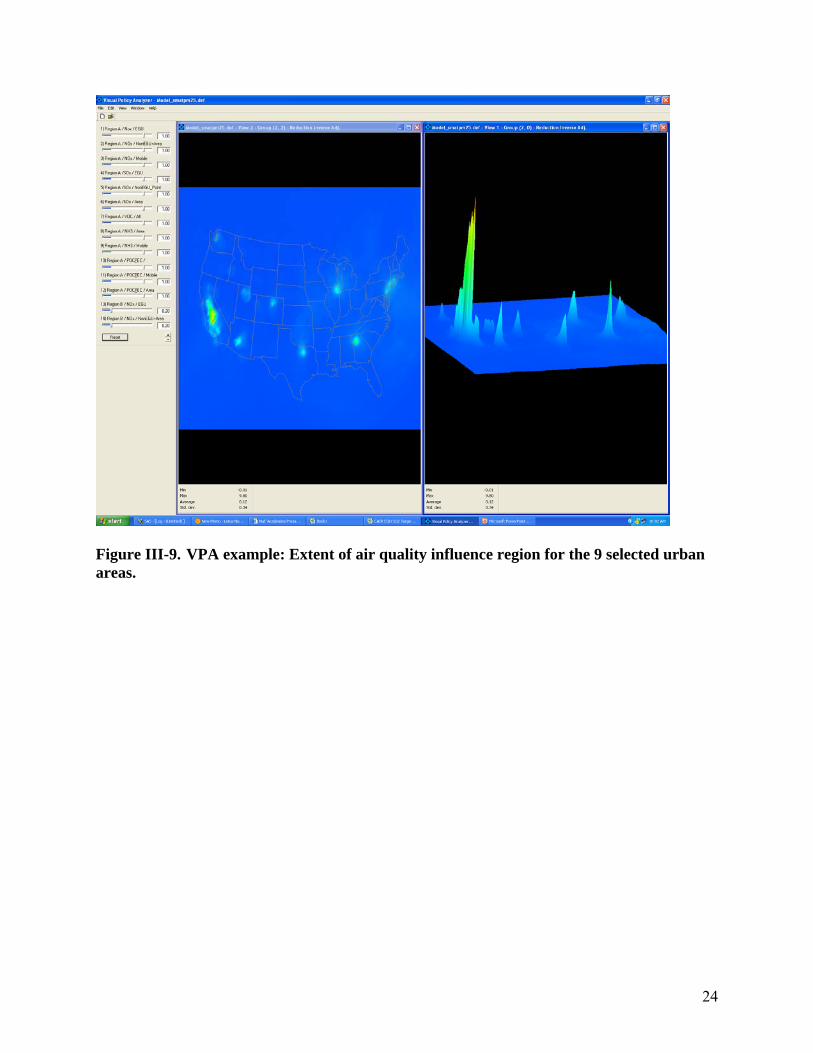
B.6 Selection of Regional vs. Local Impact Based on the selection of 12 control factors, the RSM experimental design applied a regional design allowing for development of independent response surfaces for particular urban areas, as well as a generalized response surface (i.e. air quality response) for all other locations (outside of the particular urban areas). A rigorous area-of-influence analysis was conducted for the selection of RSM urban locations to discern the degree of overlap between different urban areas in terms of air quality impacts, and to tease out local versus regional impacts. The area-of-influence analysis incorporated control model runs where emissions were zeroed out in many urban areas. Results of these control runs for the months of February and July are shown in Figures III-4 and III-5. The area-of-influence analysis concluded that ambient PM2.5 in each of the 9 urban areas is largely independent of the precursor emissions in all other included urban areas. This conclusion is also supported and clearly seen in Figure III-9 (demonstrating the extent of the air quality influence region), where reductions (represented as spikes in figure display) of PM2.5 based on an example of local precursor controls are shown. Thus, selection of these areas allows the RSM to analyze air quality changes in these 9 urban areas and associated counties independent of one another. These 9 urban areas include New York / Philadelphia (combined), Chicago, Atlanta, Dallas, San Joaquin, Salt Lake City, Phoenix, Seattle, and Denver. Figure III-6 displays these 9 urban areas based on the CMAQ model 36-km grids.

11 The data in Figure III-3, which are based on the emissions inventory developed for CAIR, suggest EGUs contribute on the order of 10% of primary organic carbon. More recently, EPA has reviewed data on primary EGU emissions and concluded these estimates are approximately an order of magnitude too high. This suggests that the control costs and reductions associated with any controls for EGU POC in are of little relevance. EPA has since corrected this portion of the inventory for future analyses and modeling.

17

Figure III-4. PM2.5: Areas of influence for nine selected RSM urban locations for the monthly average of July 2001.

Figure III-5. PM2.5: Areas of influence for nine selected RSM urban locations for the monthly average of February 2001.

18

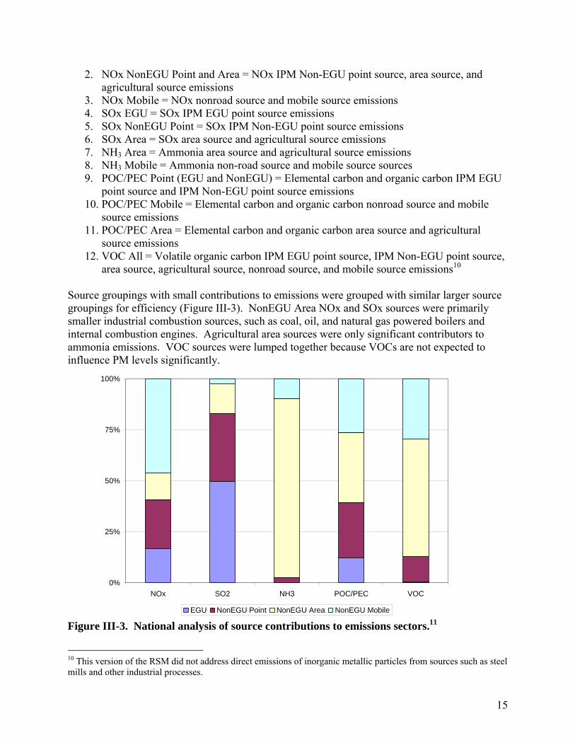
Figure III-6. Map of the CMAQ modeled 36-km grids for nine urban areas modeled. B.7 Output Metrics for CMAQ RSM PM2.5 Several output measures of PM2.5 levels were extracted from the CMAQ model runs which are of particular interest for this PM NAAQS RIA. The quarterly mean and annual 98th percentile daily average of sulfate, nitrate, crustal, elemental carbon, organic carbon, and ammonium concentrations were outputted to influence development of RSM surfaces. Projected PM2.5 annual and daily design values at monitored locations were used to assess how the attainment status of an area might be affected by different control strategies. In general, the procedures for projecting both the annual and daily PM2.5 design values are based on using model predictions in a relative sense. In this manner, the 2001 Base Year predictions and the 2015 future predictions are coupled with ambient data to forecast future concentrations. This approach is consistent with the EPA draft guidance documents for modeling PM2.5.12 Projected annual design values were calculated using the Speciated Modeled Attainment Test (SMAT) approach, the details of which can be found in the report "Procedures for Estimating Future PM2.5 Values for the CAIR Final Rule by Application of the (Revised) Speciated Modeled

12 U.S. Environmental Protection Agency, 2001. Draft Guidance on the Use of Models and Other Analyses in Attainment Demonstrations for the PM2.5 NAAQS.

19

Attainment Test (SMAT)".13 Below are the steps we followed for projecting future PM2.5 concentrations. These steps were performed to estimate future case concentrations at each FRM monitoring site. The starting point for these projections is the average of the 1999-2001, 2000-2002, and 2001-2003 design values at each monitoring site. By averaging 1999-2001, 2000-2002, and 2001-2003, the value from 2001 is weighted three times, whereas, values for 2000 and 2002 are each weighted twice, and 1999 and 2003 are each weighted once. This approach has the desired benefits of (1) weighting the PM2.5 values towards the middle year of the five-year period, which is the 2001 Base Year for our emissions projections, and (2) smoothing out the effects of year-to-year variability in emissions and meteorology that occurs over the full five-year period. This approach provides a robust estimate of current air quality for use as a basis for future year projections.

Step 1: Calculate quarterly mean ambient concentrations for each of the six major components of PM2.5 (i.e., sulfate, nitrate, ammonium, elemental carbon, organic carbon, and crustal material) using the component species concentrations estimated for each FRM site and estimate the species fractions at each FRM site, then multiply the average 1999-2003 FRM quarterly mean concentration at each site by the estimated fractional composition of PM2.5 species, by quarter (e.g., 20 percent sulfate multiplied by 15.0 µg/m3 of PM2.5 equals 3 µg/m3 sulfate). Step 2: Calculate quarterly average Relative Reduction Factors (RRFs) for sulfate, nitrate, elemental carbon, organic carbon, and crustal material. The species-specific RRFs for the location of each FRM are the ratio of the 2015 CAIR case to 2001 Base Year quarterly average model predicted species concentrations. The species-specific quarterly RRF are then multiplied by the corresponding 1999-2003 quarterly species concentration from Step 1. The result is the future case quarterly average concentration for each of these species. Step 3: Calculate quarterly average concentrations for ammonium and particle-bound water. The future case concentrations for ammonium are calculated using the future case sulfate and nitrate concentrations determined from Step 2 along with the degree of neutralization of sulfate (held constant from the base year). Concentrations of particle-bound water are calculated using the empirical relationship derived from the AIM model using the future case concentrations of sulfate, nitrate, and ammonium as inputs. Step 4: Calculate the mean of the four quarterly average future case concentrations to estimate future annual average concentration for each component specie. The annual average concentrations of the components are added together to obtain the future annual average concentration for PM2.5. Step 5: For counties with only one monitoring site, the projected value at that site is the future case value for that county. For counties with more than one monitor, the highest value in the county is selected as the concentration for that county.

13 U.S. Environmental Protection Agency, 2004. “Procedures for Estimating Future PM2.5 Values for the CAIR Final Rule by Application of the (Revised) Speciated Modeled Attainment Test (SMAT)- Updated 11/8/04”.

20

The daily design values are based on applying a similar projection method. As with the annual design value, monitor data for the years 1999 to 2003 are used as the basis for the projection. There are several steps in the projection for each of the base years of monitoring data:

Step 1: The first step in projecting the daily design value is to identify the maximum daily average PM2.5 concentration in each quarter that is less than or equal to the annual 98th percentile value over the entire year. Step 2: These quarterly PM2.5 concentrations are then separated into their component species by multiplying the quarterly maximum daily concentration at each site by the estimated fractional composition of PM2.5 species, by quarter, based on the observed species fractions from speciation monitors in 2002. Step 3: The component species are then projected by multiplying each species concentration by the quarterly relative reduction factors for each specie derived from the 2015 and 2001 PM2.5 air quality modeling. Step 4: The projected species components are then summed to obtain a PM2.5 concentration for each quarter that represents a potential daily design value. Step 5: The projected daily design value for each monitor in 2015 is then calculated as the maximum of the projected quarterly values.

This procedure is repeated for each of the years of monitoring data, 1999-2003. A weighted average projected 2015 design value is then calculated by averaging the projections for 3 year intervals (1999-2001, 2000-2002, 2001-2003), and then averaging over the three interval averages. The projected daily design value for a county is then calculated as the maximum weighted average design value (1999 - 2003) across all monitors within a county. In addition to the aforementioned PM2.5 metrics, other outputs were extracted however; they are not currently used for the proposed PM NAAQS RIA. These metrics include: annual and quarterly nitrogen and sulfate deposition, annual mean of visibility (light extinction coefficient of the average 20% worst days, average of 20% best days), daily one-hour ozone maximum, 12-hour daylight average ozone, and daily 24-hour average ozone. The following is the translation of CMAQ output species into PM2.5 and related species (units= µg/m3): PM2.5 mass: PM2.5 = ASO4I + ASO4J + ANH4I + ANH4J +

ANO3I +ANO3J + AORGAI + AORGAJ + 1.167*AORGPAI + 1.167*AORGPAJ+

AORGBI + AORGBJ + AECI + AECJ + A25I + A25J Sulfate PM: PM_SULF = ASO4I + ASO4J Nitrate PM: PM_NITR = ANO3I + ANO3J Ammonium PM: PM_AMM = ANH4I + ANH4J Organic aerosols: PM_ORG_TOT = AORGAI + AORGAJ + 1.167*AORGPAI +

21

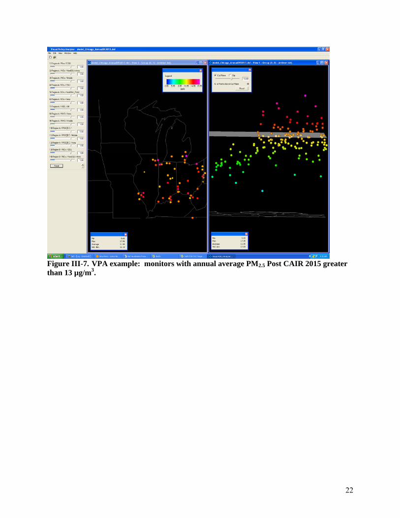
1.167*AORGPAJ + AORGBI + AORGBJ Elemental Carbon: PM_EC = AECI + AECJ Crustal Material (soils): PM_OTH = A25I +A25J Coarse PM: PM_COARS = ASOIL +ACORS + ASEAS where, PM_SULF is particulate sulfate ion, ASO4J is accumulation mode sulfate mass, ASO4I is aitken mode sulfate mass, PM_NITR is particulate nitrate ion, ANO3J is accumulation mode nitrate mass, ANO3I is aitken mode aerosol nitrate mass, ANH4J is accumulation mode ammonium mass, ANH4I is aitken mode ammonium mass, PM_ORG_TOT is total organic aerosols, AORGAJ is accumulation mode anthropogenic secondary organic mass, AORGAI is aitken mode anthropogenic secondary organic mass, AORGPAJ is accumulation mode primary organic mass, AORGPAI is aitken mode primary organic mass, AORGBJ is accumulation mode secondary biogenic organic mass, AORGBI is aitken mode biogenic secondary biogenic organic mass, PM_EC is primary elemental carbon, AECJ is accumulation mode elemental carbon mass, AECI is aitken mode elemental carbon mass, PM_OTH is primary fine particles (other unspeciated primary PM2.5), A25J is accumulation mode unspecified anthropogenic mass, A25I is aitken mode unspecified anthropogenic mass. PM2.5 is defined as the sum of the individual species. Note that a factor of 1.167 was applied to AORGPAI and AORGPAJ since the CMAQ model assumed the conversion factor between organic carbon to organic mass is 1.2 for primary organic aerosol emission and measurements assumed the conversion factor of 1.4. B.8 RSM Graphical Tool: Visual Policy Analyzer The RSM will be part of an integrated suite of 3 distinct tools, the Air Strategy Assessment Program (ASAP) which EPA is creating. ASAP uses a systematic approach for linking data and models for integrated assessments. This suite of tools is intended to facilitate multipollutant screening analyses of multiple air quality control strategies. ASAP serves as a graphical user interface that allows for easy inputs by the user with simultaneous analysis features (graphs and maps). RSM provides information on air quality responses to reductions of pollutants for various sectors. Within the ASAP framework, RSM provides this information in the form of graphical displays: bar charts, pollutant/sector stacked bar charts, and histograms. The Visual Policy Analyzer (VPA) tool was developed as a graphically based analysis tool for interacting with the RSM. The VPA tool functions outside of the ASAP framework. The VPA allows for simultaneous viewing of inputs of emissions changes on multiple model outputs. For example, the user will be able to change any policy factor (e.g., mobile NOx levels) and see the impact on PM2.5 constituents (PM sulfate, PM nitrate, etc.). The future design and advancements of the VPA will be implemented to include real-time interaction with ozone, visibility, and deposition. Figures III-7 – III-9 display example outputs of the VPA.

22

Figure III-7. VPA example: monitors with annual average PM2.5 Post CAIR 2015 greater than 13 µg/m3.

23

Figure III-8. VPA example: Monitors with annual average PM2.5 Post CAIR 2015 greater than 13 µg/m3 after applying 50 percent reduction in carbon.

24

Figure III-9. VPA example: Extent of air quality influence region for the 9 selected urban areas.

25

IV. Validation of the Response Surface Modeling To develop a response surface approximation to CMAQ, a multidimensional kriging approach was implemented. The RSM uses a nonlinear 24-dimensional kriging model implemented through SAS (2005)14 software. Kriging is an interpolation method based on an exponentially weighted sum of the sample data. This modeling approach is appropriate for data generated using a non-stochastic computer model, and can approximate highly nonlinear surfaces as long as they are locally continuous. The predicted changes in PM2.5 in each CMAQ grid cell was modeled as a function of the weighted average of the modeled responses in the experimental design. The weight assigned to a particular modeled output depends on the Euclidean distance between the factor levels defining the policy to be predicted and the factor levels defining the CMAQ experimental run.15 Uncertainties associated with RSM come from two key areas: (1) inherent uncertainties from the air quality model (CMAQ) due to uncertainties of modeling sciences and formulation, computational approximation, and input data, including both emission and meteorological data; and (2) statistical representation of RSM model to simulate the responses of the air quality model (CMAQ) due to preset control scenarios. The model was validated using a number of techniques, while recognizing and acknowledging these uncertainties associated with the development and application of the RSM. Visual inspection of prediction maps was conducted to confirm overall spatial comparability in the predicted versus modeled outputs for each of the CMAQ experimental design runs. Cross-validation was used to evaluate overall response-surface performance. For each iterative run, one of the experimental model runs is left out of the model estimation, and the RSM is then computed and used to predict the omitted run. RSM predicted changes in PM2.5 air quality are compared with CMAQ predictions and a standard set of model performance evaluation metrics over all grid cells is computed for the run. These evaluation metrics include: bias, error, normalized bias and error, and fractional bias and error.16 The performance metrics are defined as follows: (3) YyBIAS −= ˆ (4) YyERROR −= ˆ

14 SAS Institute, 2005. SAS Online Doc© 9.1.3. Accessed online at http://support.sas.com/onlinedoc/913/docMainpage.jsp 15 Hubbell, B.J., Dolwick, P.D., Mooney, D., Morara, M., 2005. Evaluating the relative effectiveness of ozone precursor controls: Design of computer experiments applied to the comprehensive air quality model with extensions (CAMx), Air and Waste Management Association Conference Proceedings. 16 Boylan, J.W. Evaluation of Model Performance. Presentation for the 3rd Particulate Matter/Regional Haze/Ozone Modeling Workshop, New Orleans, LA, May 19, 2005. Accessed online at: http://cleanairinfo.com/modelingworkshop/presentations/PM_MPE_Boylan.pdf

26

(5) Y

YyBIASNORMALIZED −=

ˆ

(6) Y

YyERRORNORMALIZED −=

ˆ

(7) ⎟⎠⎞

⎜⎝⎛ +

−=

2ˆˆ

YyYyBIASFRACTIONAL (bounded between -200% and +200%)

(8) ⎟⎠⎞

⎜⎝⎛ +

−=

2ˆˆ

YyYy

ERRORFRACTIONAL (bounded between 0% and +200%)

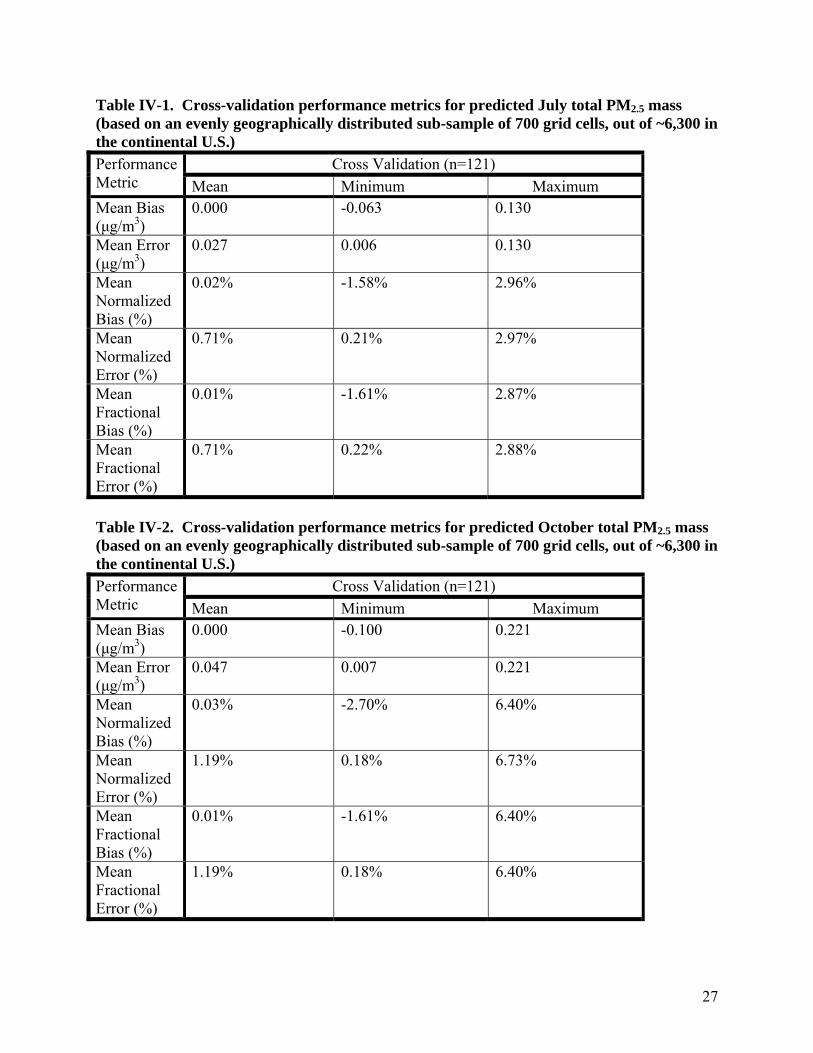
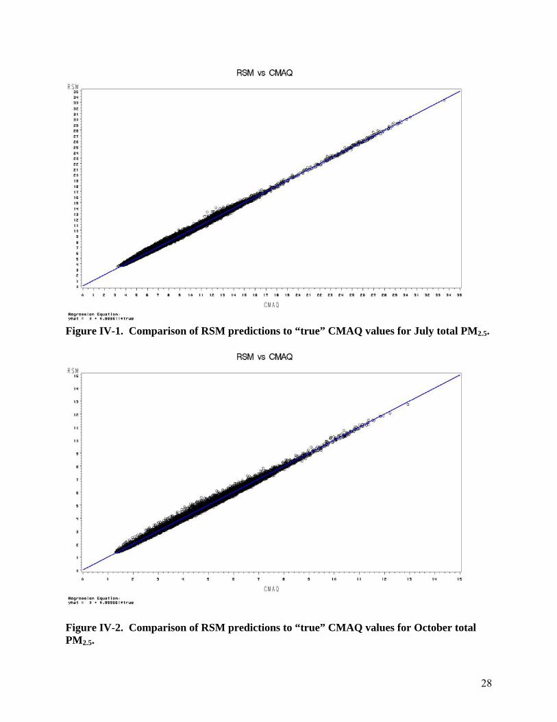
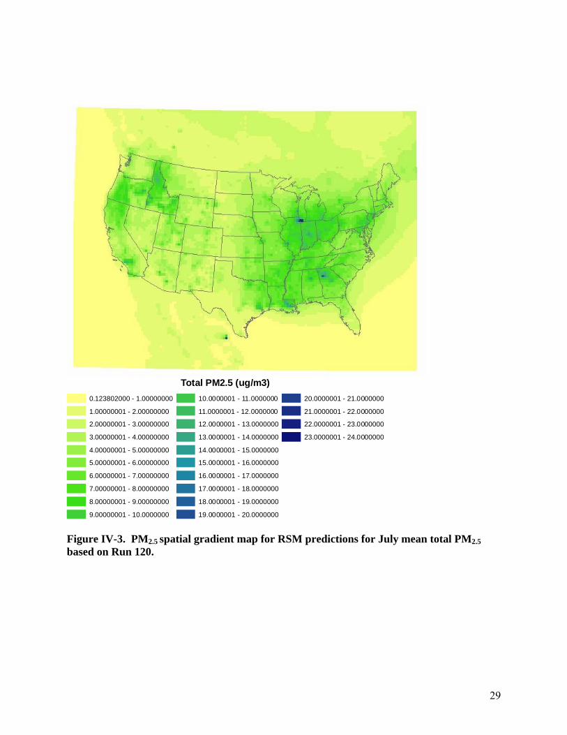
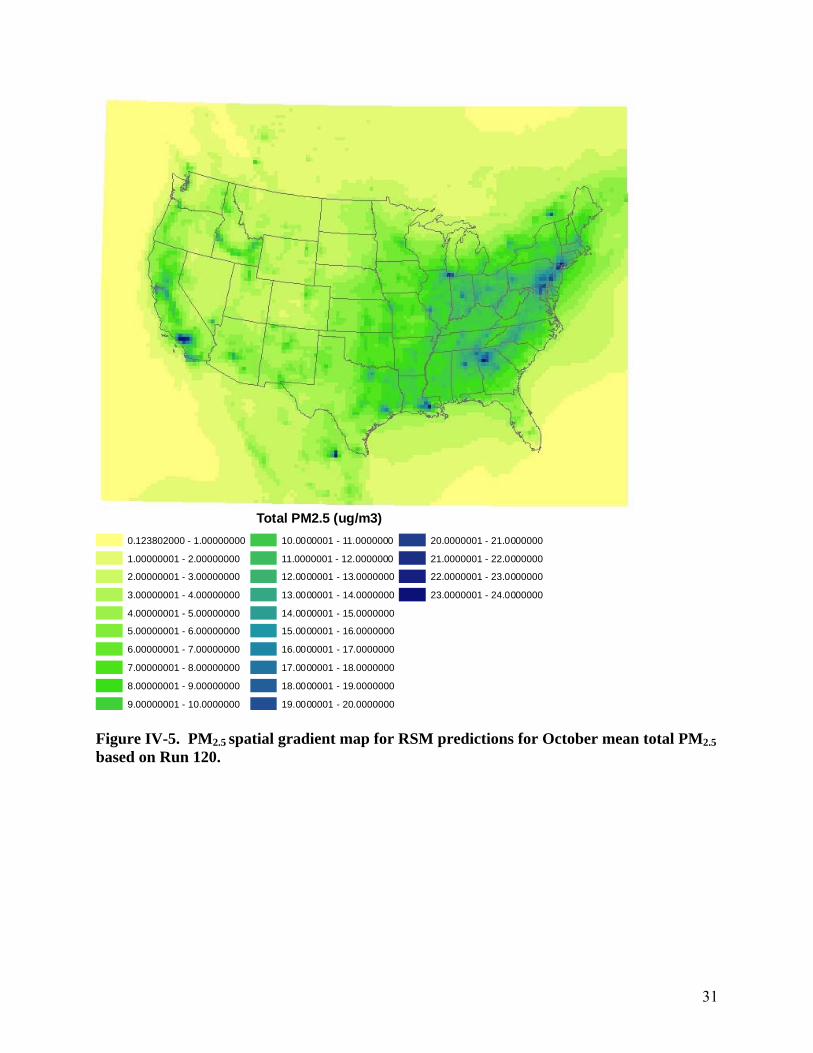
The process is then repeated for each experimental design model run, and the distributions of the performance metrics are then examined over the total number of model runs to gauge the overall performance of the response surface across the experimental design. During the beginning stages of the RSM evaluation, an initial cross-validation was performed for selected corresponding CMAQ and RSM grid cells for the months of July and October (Tables IV-1 and IV-2). Comparison of RSM predictions to “true” CMAQ values for July and October total PM2.5 show good agreement (Figures IV-1 and IV-2). In addition, comparison of RSM and CMAQ predictions for the July mean total PM2.5 for a particular run (run 120) is shown in Figures IV-3 and IV-4. Likewise, Figures IV-5 and IV-6 display a comparison of RSM and CMAQ predictions for October mean total PM2.5 for run 120.

27

Table IV-1. Cross-validation performance metrics for predicted July total PM2.5 mass (based on an evenly geographically distributed sub-sample of 700 grid cells, out of ~6,300 in the continental U.S.)

Cross Validation (n=121) Performance Metric Mean Minimum Maximum Mean Bias (µg/m3)

0.000 -0.063 0.130

Mean Error (µg/m3)

0.027 0.006 0.130

Mean Normalized Bias (%)

0.02% -1.58% 2.96%

Mean Normalized Error (%)

0.71% 0.21% 2.97%

Mean Fractional Bias (%)

0.01% -1.61% 2.87%

Mean Fractional Error (%)

0.71% 0.22% 2.88%

Table IV-2. Cross-validation performance metrics for predicted October total PM2.5 mass (based on an evenly geographically distributed sub-sample of 700 grid cells, out of ~6,300 in the continental U.S.)

Cross Validation (n=121) Performance Metric Mean Minimum Maximum Mean Bias (µg/m3)

0.000 -0.100 0.221

Mean Error (µg/m3)

0.047 0.007 0.221


0.03% -2.70% 6.40%


1.19% 0.18% 6.73%


0.01% -1.61% 6.40%


1.19% 0.18% 6.40%

28

Figure IV-1. Comparison of RSM predictions to “true” CMAQ values for July total PM2.5.

Figure IV-2. Comparison of RSM predictions to “true” CMAQ values for October total PM2.5.

29

Figure IV-3. PM2.5 spatial gradient map for RSM predictions for July mean total PM2.5 based on Run 120.

Total PM2.5 (ug/m3)0.123802000 - 1.00000000

1.00000001 - 2.00000000

2.00000001 - 3.00000000

3.00000001 - 4.00000000

4.00000001 - 5.00000000

5.00000001 - 6.00000000

6.00000001 - 7.00000000

7.00000001 - 8.00000000

8.00000001 - 9.00000000

9.00000001 - 10.0000000

10.0000001 - 11.0000000

11.0000001 - 12.0000000

12.0000001 - 13.0000000

13.0000001 - 14.0000000

14.0000001 - 15.0000000

15.0000001 - 16.0000000

16.0000001 - 17.0000000

17.0000001 - 18.0000000

18.0000001 - 19.0000000

19.0000001 - 20.0000000

20.0000001 - 21.0000000

21.0000001 - 22.0000000

22.0000001 - 23.0000000

23.0000001 - 24.0000000

30

Figure IV-4. PM2.5 spatial gradient map for CMAQ simulations for July mean total PM2.5 based on Run 120.

Total PM2.5 (ug/m3)0.123802000 - 1.00000000

1.00000001 - 2.00000000

2.00000001 - 3.00000000

3.00000001 - 4.00000000

4.00000001 - 5.00000000

5.00000001 - 6.00000000

6.00000001 - 7.00000000

7.00000001 - 8.00000000

8.00000001 - 9.00000000

9.00000001 - 10.0000000

10.0000001 - 11.0000000

11.0000001 - 12.0000000

12.0000001 - 13.0000000

13.0000001 - 14.0000000

14.0000001 - 15.0000000

15.0000001 - 16.0000000

16.0000001 - 17.0000000

17.0000001 - 18.0000000

18.0000001 - 19.0000000

19.0000001 - 20.0000000

20.0000001 - 21.0000000

21.0000001 - 22.0000000

22.0000001 - 23.0000000

23.0000001 - 24.0000000

31

Figure IV-5. PM2.5 spatial gradient map for RSM predictions for October mean total PM2.5 based on Run 120.

Total PM2.5 (ug/m3)0.123802000 - 1.00000000

1.00000001 - 2.00000000

2.00000001 - 3.00000000

3.00000001 - 4.00000000

4.00000001 - 5.00000000

5.00000001 - 6.00000000

6.00000001 - 7.00000000

7.00000001 - 8.00000000

8.00000001 - 9.00000000

9.00000001 - 10.0000000

10.0000001 - 11.0000000

11.0000001 - 12.0000000

12.0000001 - 13.0000000

13.0000001 - 14.0000000

14.0000001 - 15.0000000

15.0000001 - 16.0000000

16.0000001 - 17.0000000

17.0000001 - 18.0000000

18.0000001 - 19.0000000

19.0000001 - 20.0000000

20.0000001 - 21.0000000

21.0000001 - 22.0000000

22.0000001 - 23.0000000

23.0000001 - 24.0000000

32

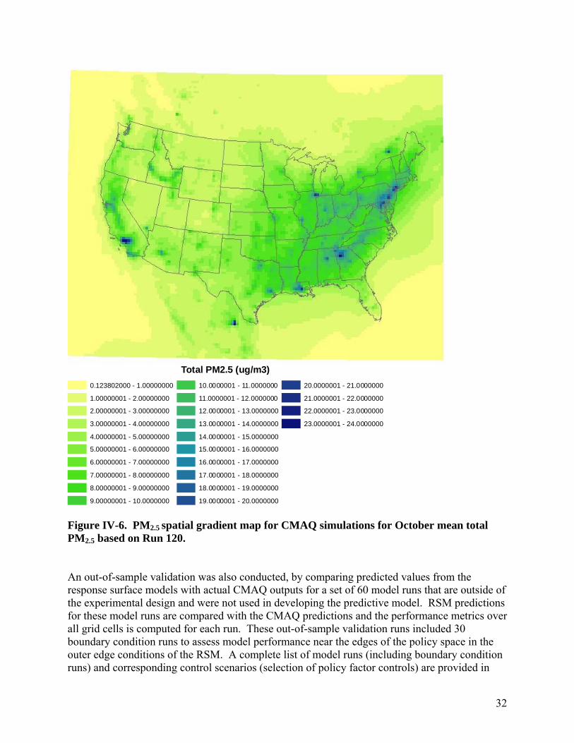
Figure IV-6. PM2.5 spatial gradient map for CMAQ simulations for October mean total PM2.5 based on Run 120. An out-of-sample validation was also conducted, by comparing predicted values from the response surface models with actual CMAQ outputs for a set of 60 model runs that are outside of the experimental design and were not used in developing the predictive model. RSM predictions for these model runs are compared with the CMAQ predictions and the performance metrics over all grid cells is computed for each run. These out-of-sample validation runs included 30 boundary condition runs to assess model performance near the edges of the policy space in the outer edge conditions of the RSM. A complete list of model runs (including boundary condition runs) and corresponding control scenarios (selection of policy factor controls) are provided in

Total PM2.5 (ug/m3)0.123802000 - 1.00000000

1.00000001 - 2.00000000

2.00000001 - 3.00000000

3.00000001 - 4.00000000

4.00000001 - 5.00000000

5.00000001 - 6.00000000

6.00000001 - 7.00000000

7.00000001 - 8.00000000

8.00000001 - 9.00000000

9.00000001 - 10.0000000

10.0000001 - 11.0000000

11.0000001 - 12.0000000

12.0000001 - 13.0000000

13.0000001 - 14.0000000

14.0000001 - 15.0000000

15.0000001 - 16.0000000

16.0000001 - 17.0000000

17.0000001 - 18.0000000

18.0000001 - 19.0000000

19.0000001 - 20.0000000

20.0000001 - 21.0000000

21.0000001 - 22.0000000

22.0000001 - 23.0000000

23.0000001 - 24.0000000

33

Appendix B. The distribution of the performance metrics over the set of 60 runs was then examined. Cross-validation and out-of-sample performance metrics for the PM2.5 design value metric are shown in Table IV-3. Table IV-3. Cross Validation Performance Metrics for the Predicted PM2.5 Design Values

Daily 98th Percentile Design Value Annual Mean Design Value Performance Metric Mean Minimum Maximum Mean Minimum Maximum Mean Bias (µg/m3)

0.001 -0.646 0.796 0.001 -0.136 0.333

Mean Error (µg/m3)

0.282 0.147 0.822 0.067 0.021 0.336


0.03% -2.51% 2.81% 0.03% -1.51% 2.86%


1.13% 0.57% 3.10% 0.71% 0.21% 2.95%


0.02% -2.62% 2.74% 0.02% -1.51% 2.86%


1.14% 0.58% 3.19% 0.71% 0.21% 2.90%



Appendix A

Control Scenario Model Runs



Stage Run Number

1) region A / NOx / EGU

2) region A / NOx /

NonEGU+Area

3) region A / NOx / Mobile

4) region A /SOx / EGU

5) region A /SOx /

NonEGU_Point

6) region A /SOx / Area

7) region A / VOC / All

8) region A / NH3 / Area

9) region A / NH3 / Mobile

10) region A / POC&PEC /

EGU+NonEGU


Mobile


Area

X1 X2 X3 X4 X5 X6 X7 X8 X9 X10 X11 X121 1 1.0000000 1.0000000 1.0000000 1.0000000 1.0000000 1.0000000 1.0000000 1.0000000 1.0000000 1.0000000 1.0000000 1.00000001 2 0.8917761 1.0202863 0.8305486 0.9630258 0.8759180 0.9027776 0.1706268 0.1743507 0.9938867 0.3943875 0.9089606 0.87647951 3 0.5757257 0.2660104 1.0219009 0.5561090 0.2476034 0.8032814 0.6175011 1.0011361 0.0245822 0.5016423 1.1284927 0.52022081 4 0.0613440 0.4620605 0.5055674 0.3992450 0.9646536 1.1373681 0.8193273 0.6693372 0.4947579 0.6882374 1.0815584 0.49674141 5 0.2962200 0.6071276 0.7457047 0.0658980 0.5813182 0.4308903 1.0586252 1.0753493 0.6384797 0.9133312 0.5117359 0.64017001 6 0.1199474 1.1633908 0.7550934 0.2867301 0.8007379 0.3532581 0.4078587 0.8255346 0.9113647 0.8460796 0.7986134 1.13878531 7 0.4247985 0.9874206 0.6074017 1.1943385 1.1751841 0.3369149 0.3017320 0.0281063 0.7755347 0.0526044 0.3549848 0.27777011 8 1.1458733 0.5388726 1.1261608 1.0325960 0.0478220 0.6617708 0.6461682 0.6382648 0.3720081 0.7545740 0.3602044 0.08831701 9 0.3873795 0.7013402 0.4592687 0.1587126 0.6229901 1.0868247 0.5205359 0.9277289 0.7860278 0.1667150 0.8179027 0.10401591 10 0.3445258 1.1720162 0.8929441 0.4312985 1.1927137 0.5639167 0.3490241 1.1554275 0.6875944 0.2780773 0.5307151 0.78135371 11 0.0831331 0.7171276 0.4702332 0.9338521 0.6777555 0.8583126 0.1612429 0.9120252 0.9664511 0.2626853 0.0035322 0.32973231 12 0.1297348 1.0038537 0.8037916 0.1345442 0.5095891 0.1500031 1.1026635 0.2254651 0.1587382 0.5236595 0.6082176 0.15560281 13 0.3537135 0.8882669 0.9703029 0.9815889 0.1840197 0.5745094 0.1507981 1.0435884 1.0565935 0.4883080 0.9752145 0.12127551 14 1.1137550 0.0386481 0.2879607 0.7883295 0.4710581 0.3997246 0.9244416 0.6407529 0.2015128 0.2894022 0.1201472 0.41021051 15 1.1541664 0.4285464 0.7853174 1.0413543 0.9215108 0.4246917 0.0239380 0.1382198 0.2245466 1.1870604 0.4396621 0.50579661 16 1.0631307 0.8069088 0.9565155 0.3542480 0.0813060 0.3874497 0.0500384 1.1329369 1.0675565 0.3404673 0.5032608 0.98062131 17 0.0598692 0.7723593 1.0605714 1.0943860 1.0045519 0.1325842 0.0627904 0.9959790 0.3425626 1.0221077 0.5531616 0.97267851 18 0.0700900 0.1583829 1.1926875 0.0149045 0.5260646 0.9138528 0.9083484 0.4941159 0.5142014 1.0792261 1.0086657 0.39546381 19 1.0172755 0.9267110 0.0172941 0.8151985 0.3392861 0.8756710 0.4521253 0.7092411 0.8220213 0.8972647 0.1789215 0.66129511 20 1.1205631 0.5795498 0.2622965 1.1800852 0.0998920 0.8693987 0.4817324 0.9842759 0.4744441 0.7931610 0.6682863 0.47830851 21 0.8240074 0.0207781 0.5954154 0.9230984 0.2156308 0.4793842 0.5533555 1.0354790 0.5061000 0.0866735 0.6814743 1.15066311 22 1.1804455 0.2833504 0.4495181 0.2631563 0.6133755 1.1290661 0.4154074 0.0408373 0.4873830 1.1971353 0.5922452 1.19072281 23 0.7665640 1.0552730 1.0089826 0.8384905 0.2754498 0.5551943 0.4220539 0.5360028 0.2492605 0.8741171 0.3090030 1.07460461 24 0.7518466 0.1871500 0.4674471 0.1413659 0.4530526 0.2603812 1.1679122 0.0128813 0.7473027 0.7827610 0.2907536 1.17032911 25 0.1005391 0.9607032 1.1135169 0.1766030 0.6648941 1.0764599 0.7202375 0.2335426 0.5465157 0.1707806 0.1447755 0.77236911 26 0.2700999 0.5017904 0.2149969 0.8061909 0.4981132 0.6518806 0.3176568 0.0970426 0.2334024 1.1454820 1.1315173 0.90840071 27 0.5038364 0.0127421 0.3599027 0.7143260 0.8140581 0.0626248 0.5709524 0.8527188 0.1151996 1.0950342 1.1007156 0.03071511 28 0.5972388 0.4041907 0.2250784 1.1351703 0.4125801 0.7485700 0.1867574 0.2946766 1.1523924 0.2237699 0.9563971 0.40230401 29 0.4328085 0.9581458 0.1216657 0.0745722 0.4269842 0.6081415 0.6318056 0.8055940 0.0684980 0.9770143 0.2773692 0.63678841 30 0.8518393 0.3212539 1.1831085 0.4805996 0.3087242 0.7637074 0.2738558 0.6595938 0.4182312 1.1223065 1.0682915 0.53555561 31 0.8811701 0.5632910 1.0925999 0.5324414 0.5632229 0.5960226 1.1887516 0.6270556 1.0207483 0.9488535 0.8352504 1.14852721 32 0.5104390 0.6467937 0.3669776 0.7091419 1.1038441 1.1701880 0.0330265 0.8898659 0.3691453 0.0251029 0.6278800 0.95145451 33 0.1889664 0.8179359 0.2020374 0.4545032 0.1590509 0.0857378 0.3835675 0.8381442 0.2707743 0.5315828 1.1668311 0.23802871 34 0.2224134 1.0190370 0.6208698 0.6959477 0.4848133 1.0083507 1.0292833 0.2682756 0.8325972 0.9915035 0.2802922 0.22399941 35 0.5891162 0.7417753 0.8894118 0.4956199 0.5734597 0.2534253 0.9833746 0.1870750 1.1370610 0.0782513 0.2689955 0.75110641 36 1.1694108 0.8662052 0.8103384 0.7248794 0.4381039 0.2265009 0.9900426 0.7762748 0.7056527 0.6326106 0.8524845 0.31103721 37 0.4786493 0.0803770 0.1401505 0.6207126 0.9309039 0.7569876 0.1321892 0.8728087 1.0366710 0.8111077 0.4155347 0.04128811 38 1.0381828 0.5210140 0.5787255 0.6484217 1.0965850 0.5235299 0.1029370 0.7636911 1.1889260 1.0622932 0.5629322 0.54501111 39 0.5259089 0.9105050 0.5163236 0.1281554 0.1208996 0.8207130 0.5662090 0.3272207 0.5661943 0.3503184 0.8011908 0.30375401 40 0.2831007 0.6241930 0.0372872 0.8940811 0.2228235 0.2809300 0.5134552 0.0581287 0.8191113 1.0055698 1.0225226 0.13131781 41 1.0287964 0.3141985 0.9094615 0.3373115 1.1534533 0.3290696 0.5989086 0.8107954 0.6405617 0.8019855 0.9433654 0.11911801 42 1.0537317 0.4789060 0.4049424 0.3210719 0.9430135 0.1899415 1.1215001 0.0752256 0.7957731 0.3289370 1.0735120 0.46527461 43 0.6838139 0.4554747 0.2796927 0.1034354 0.0352487 0.6985866 0.2499764 0.6089464 0.3251546 0.6118472 0.8624567 0.26231861 44 0.2380314 0.2044139 0.1590749 0.9405089 0.6559679 0.5364115 0.5364816 0.3614354 0.4609214 0.1856151 0.0442942 1.02408031 45 0.2695817 0.5870485 0.3116595 0.0405774 1.0297623 0.7322556 0.8988894 1.0190603 0.3999124 0.7616646 0.4222136 0.51765461 46 0.8434046 0.8466314 0.4187904 0.8209990 0.8397281 1.0233317 0.0009577 0.9604678 0.6120980 0.8678461 0.1941893 0.84888241 47 0.0215039 0.3812900 0.1824253 0.9596480 0.2092466 0.3100773 0.8064858 1.1220847 0.4477197 0.5636838 0.3235395 0.48118121 48 0.6383915 0.0668246 0.7323819 0.3490295 0.5373391 1.1954418 0.7031401 0.1051663 0.4535415 0.8588324 0.0258331 0.7602727

Region A Emission Control Factors

Stage Run Number


2) region A / NOx /

NonEGU+Area



5) region A /SOx /

NonEGU_Point






EGU+NonEGU


Mobile


Area

X1 X2 X3 X4 X5 X6 X7 X8 X9 X10 X11 X121 49 0.6663152 0.2149013 1.0871995 0.9100780 0.8839803 0.5817384 0.8868249 0.9061724 0.9491932 0.7252542 0.2290034 0.06188751 50 0.8328004 0.4341146 0.3920387 0.6714147 0.7148296 0.1955624 0.3706591 0.5420089 0.0782005 0.6522027 0.4684685 0.07045301 51 0.8119017 0.7605139 0.0541995 0.0530866 0.7428447 1.1149914 0.6068168 0.1140219 0.2526379 0.3728624 0.4881348 0.35778001 52 0.6228721 0.9774031 0.5873336 1.1641807 0.9872529 0.9443085 0.9635871 0.3194205 0.0554524 0.2447167 0.7792361 0.01129951 53 0.7308682 0.7322445 1.1661770 0.4112820 0.0672677 1.1404016 0.4693613 0.0314736 0.6693529 0.1443893 0.8477615 0.16066621 54 0.4895296 0.1297654 0.3249296 0.1969896 0.7387391 0.6300886 1.1786541 0.1298038 1.0025562 0.7799321 0.7560902 1.09263071 55 1.1921247 0.3691076 0.4872696 0.6500148 0.1426367 1.0920806 0.8396394 0.4674217 1.1218152 0.0319902 1.0326448 0.70282451 56 0.2098407 0.1688392 0.9488572 0.7360461 1.1329632 0.9275146 0.8549835 0.4311617 0.1324523 0.0479483 0.4963420 0.59652211 57 0.3640807 1.1572095 0.6130332 0.4435378 0.5109628 0.7819728 0.7554668 0.3874395 0.0319266 0.8238777 0.8200016 0.62665341 58 0.7237567 0.2257261 1.0781659 1.1420906 1.0615598 0.4538135 1.0076114 0.3487967 0.7610389 0.0931030 1.1920183 1.00051681 59 0.0408059 0.5439352 0.8727179 0.8780372 0.1938023 0.9938209 0.2328264 0.9547506 0.9360789 1.1565083 0.2086519 0.73796951 60 0.0063165 0.6588181 0.7687972 0.8610497 0.8911062 0.8850389 0.7315817 0.8987250 0.1935107 0.9826256 1.1723043 1.01258361 61 0.5421242 0.3357983 0.0661583 0.2502053 0.2975602 0.1417516 0.6907296 0.4244070 0.8807553 1.1761539 0.1598064 0.19537551 62 0.9739873 0.8719553 0.3384258 0.0937403 0.4682085 0.5151328 0.6244480 1.1987316 1.0754747 0.0080142 0.6300319 0.43836551 63 0.3225316 0.1454780 0.6434772 0.6183074 0.0581454 0.1137857 0.6756461 0.7849608 0.3189201 0.2382126 0.4052683 0.83240341 64 0.3738117 0.7826970 0.9110874 1.0596536 0.1188078 0.5473746 0.9769619 0.1553987 0.5583492 1.1360645 0.7483689 0.99279691 65 0.9809097 0.1054644 0.7799894 0.6073199 0.3834382 0.2481087 0.6851289 0.5731044 0.5901128 0.4261334 1.1142252 0.60774501 66 0.2537007 0.6769949 0.3086453 0.5249976 0.4456382 1.1547320 0.9421302 0.4752612 1.0929866 1.1064464 0.9331393 0.33882831 67 1.0798321 1.1066956 0.8505934 0.0886270 1.0176367 0.9502497 0.7426627 0.6175206 1.0442326 0.9676803 0.5744645 0.05787171 68 0.9502494 0.9435204 0.1398165 0.7570034 1.1853942 0.4178427 1.1545824 0.4060686 0.3889284 0.9326503 0.3989056 0.21538051 69 0.2433527 0.1326575 0.2994783 1.1789594 0.1711640 0.2308714 0.7921458 1.0875786 0.4342156 1.0409151 0.4786223 0.88890751 70 0.3083376 0.1990203 0.3869307 0.5842429 0.7854696 0.7783076 1.0776650 0.9483175 0.8986668 0.2175257 0.3779711 0.94690601 71 0.0900046 0.5966515 0.3489464 0.5102866 0.0055573 0.4845883 1.1126935 0.7594511 0.6006217 0.5123451 0.7605780 0.28934591 72 0.4034348 1.0688699 0.1942316 0.6874835 0.3926585 0.6748714 1.0384085 0.5639237 1.0113362 1.0880111 0.8960362 0.86065611 73 1.1731050 0.6383467 0.8436304 0.5493873 0.0104892 0.3033700 0.1288901 0.4869242 0.8047052 0.6003107 0.0992285 1.04330471 74 0.4643325 0.0596751 1.1312363 0.2074464 0.3662489 0.1270069 0.7849191 0.3731805 0.3509845 0.0189256 0.6579168 0.20200051 75 0.0173664 0.3422776 0.9363695 0.0306216 0.6436532 0.6877710 0.3632000 0.2732799 0.6584046 0.7149991 0.1333495 0.17711631 76 0.9002900 0.5116704 0.2572188 0.7418588 0.7554137 1.1013777 0.4911601 0.6872260 0.4026138 0.9572350 0.5288709 1.12767781 77 0.6037094 0.2547657 0.4958731 0.2261090 0.3456571 0.1799125 0.5009690 0.8631002 0.5281777 1.0397427 0.0179954 0.42308281 78 0.3104274 0.3726899 0.6512266 1.1203751 0.2804484 0.9856980 0.4332193 0.1942294 0.2954508 0.6921218 0.0747126 0.89916031 79 0.5635280 1.0305622 1.0123014 0.5715069 0.9183353 0.4437053 0.9187665 0.5988764 0.9792513 0.5761602 0.1653451 0.37031001 80 0.9940311 0.6157773 0.1730168 1.1080396 0.2626545 0.7958467 0.9555755 1.1743806 0.7120362 0.3016220 0.1033405 0.92552561 81 0.4467526 0.8321395 0.1638895 0.9743252 1.0494352 1.0376940 0.3914049 0.7281134 0.3067022 1.0160216 0.9962293 0.09224621 82 0.9244612 0.6859700 0.8293194 1.0007431 1.1153228 1.0468622 0.7759632 0.7427118 1.1061674 0.6671323 0.2134494 0.82516131 83 0.1706887 0.1155916 0.7913427 0.8524872 0.9703355 0.6273396 0.0802091 0.3358030 0.8581821 0.6719520 0.3859022 0.93804211 84 0.8036437 0.0910579 1.0579285 0.4040752 1.0888298 0.9665558 0.2274823 1.0277824 0.0482226 0.4107312 0.4542150 0.25741091 85 0.9433588 0.4117014 0.7259802 0.2960371 0.3594145 1.1832677 1.1934469 0.9388456 0.6762143 0.0692021 0.0806845 0.38236751 86 0.7859507 0.7294585 0.4200005 0.0279963 0.3140325 0.2967367 0.2099397 0.7309846 0.5868586 0.8845851 0.3304588 0.24205251 87 0.6795529 0.0763496 1.1474889 0.6313649 0.6951873 0.3788525 0.4734560 1.0941472 1.1787852 0.1952784 0.6460254 0.74297151 88 0.1480122 1.1143291 0.2388020 0.7638209 0.9024409 0.9742308 0.8787928 1.0675063 0.2164926 0.1381263 1.0524590 0.68711321 89 0.8740236 0.4920706 0.9851017 0.3832795 0.7742606 0.0467135 0.2124366 0.1461963 0.8441854 0.5568655 0.7290777 0.69008381 90 1.0972790 1.1914448 0.8638593 0.7937935 0.5530771 0.5073503 1.0653492 1.1145460 0.7337545 1.0536380 1.0973322 0.61229461 91 0.6193566 0.3566487 0.3725314 0.3062608 0.9547246 0.0337103 0.2521981 0.3929194 0.1274027 0.1005673 0.2465434 0.57431061 92 0.4538599 0.4859894 0.6338080 0.8889668 0.7299904 1.0652492 0.7674707 0.2432760 1.0893207 0.5461804 0.6775718 0.65483321 93 0.2147606 0.8552837 0.1123319 0.1882761 0.2311258 0.2755154 0.3554226 0.6912552 1.1417985 0.1274976 0.6130011 0.85659241 94 0.7735375 0.1724924 0.5572761 0.2768529 0.3291358 0.6465677 0.1109764 0.6776122 0.0194624 0.7071496 1.1531970 1.18553401 95 0.0399998 0.2398431 0.7165381 1.0895713 0.8531835 0.4619117 0.8463926 0.7903370 0.7266882 0.6244529 1.1405046 0.72074201 96 0.1664366 0.6918167 0.6681025 0.7771293 1.1207488 0.0568660 0.2964549 0.3520311 0.1781231 0.3876760 0.3158467 1.0601459


Stage Run Number


2) region A / NOx /

NonEGU+Area



5) region A /SOx /

NonEGU_Point






EGU+NonEGU


Mobile


Area

X1 X2 X3 X4 X5 X6 X7 X8 X9 X10 X11 X121 97 0.1394059 0.6689669 0.5443725 0.4602449 0.2532056 0.2114848 0.7171396 0.0072066 1.1192171 0.4529366 0.3468090 0.55694261 98 0.1945571 0.9379262 0.5285213 1.0272198 0.3710837 1.1683682 0.8664243 0.2069300 0.6286141 0.1134546 0.1152002 1.16188121 99 0.6496167 0.9044236 1.1530211 0.3680170 0.7916018 0.0191470 0.5844736 0.7179935 0.1617281 0.4796051 0.9199728 1.11292771 100 0.9611030 0.8902537 0.1017843 0.5043872 0.5439593 0.2063088 1.1456269 0.4172104 0.5310689 0.4300778 0.9807008 1.05668511 101 1.0825915 1.0953904 0.5656404 0.9098573 0.8667526 0.7242813 0.5414993 0.2546661 0.1068115 0.4402613 0.0652224 0.45226711 102 1.0440148 0.0443189 0.0760961 0.9958590 0.7079556 0.4900675 0.2677134 0.5508316 1.1666723 0.8313895 0.7044684 0.44420021 103 0.4916071 0.7598527 0.9215160 0.2127746 0.8209470 0.7197652 1.1396190 1.1671132 0.3378321 0.6438198 0.0500752 1.08945171 104 0.5336884 0.8258612 0.7092728 0.4764436 1.1688051 0.4087006 0.0110482 0.5086867 0.6929563 1.1140697 0.8848475 1.03976461 105 1.0035236 1.1851699 0.4302558 0.5662399 1.0789635 0.0744770 0.6501833 1.0556736 0.2639904 0.4977590 0.4432624 0.34359701 106 0.7076802 0.5590344 0.6885238 0.1698559 0.6341530 1.0553357 0.0702983 0.9755047 0.1892695 0.4014846 0.8741249 0.81110901 107 0.9114653 0.0089201 0.0865299 0.8493197 0.6831313 0.1021805 0.9384150 0.2105730 0.1489949 0.4672663 0.9273781 0.79689141 108 0.6948385 1.1265410 0.0024350 0.2380544 1.1453414 0.0037961 0.3212953 0.0613082 0.9022307 0.9093575 0.5805260 1.10077811 109 0.8691097 0.2711683 0.0251845 0.0097833 1.0540301 0.3421482 0.6646295 1.1470430 0.9227068 0.3620734 0.6955890 0.96760331 110 1.1038099 0.4499382 0.9964645 0.5947531 0.7646370 0.8307359 1.0820926 0.4584027 0.0957373 0.5892027 0.7899857 0.67929711 111 0.3909594 1.0493159 0.0492603 1.1588421 0.5908718 0.3603416 1.0957299 0.8419856 0.8751548 0.2510445 1.1879777 0.58460091 112 0.7111055 0.7988265 0.6796907 1.1128368 0.1389678 0.0950267 0.1401012 0.4421211 0.7573840 0.3160228 1.0416629 0.18349471 113 0.7902870 1.1430187 0.2479798 0.2447357 0.1691979 0.8425701 0.0469948 0.5171542 0.0024112 0.2090175 0.2540716 0.71933631 114 0.4182332 0.2977804 0.9662780 0.1111280 0.4014386 0.8159074 0.3352021 1.1825674 0.9512311 1.1693847 0.2393260 0.56605391 115 0.9360804 1.1308895 1.0329244 0.6689117 0.0783962 0.0244491 0.8251893 0.5231447 0.0887800 0.7440292 0.1830453 0.14148931 116 0.6563665 1.0840032 1.1740964 0.4280144 0.1090967 0.6160936 0.0909516 0.0871672 0.4295783 0.5962272 1.0119651 0.91400961 117 0.7408459 0.2400084 0.0958598 0.3759774 0.8413113 0.8909996 0.4420736 0.1696810 0.5798625 0.3393290 0.7377587 0.36306441 118 0.1599052 1.0752863 1.0454953 1.0157576 0.0227733 0.7016071 0.2849252 0.5833631 0.8602957 0.2987324 0.7127897 0.29014831 119 1.1337973 0.9967061 0.6909351 1.0718049 0.6049245 1.0194438 1.0189450 1.1087924 0.2885669 0.7304072 0.5492890 0.80598571 120 0.3399826 0.3036971 0.5358561 0.3197833 0.9926754 0.9301016 0.1994812 0.2808055 0.9889225 0.1584014 0.9690094 0.02727411 121 0.5541823 0.3999362 1.1062029 1.0637916 1.0397597 0.1631089 1.0440435 0.3071434 1.1979732 0.9227708 0.0302372 0.00587362 122 0.4347571 0.3783314 0.4394866 0.4339370 0.3764429 0.4384478 0.4345150 0.4358145 0.3797821 0.4384246 0.2477097 0.37472102 123 0.2504861 0.8488454 0.3753440 0.0004880 0.4772310 0.8499457 0.3738077 0.3733462 0.8468136 0.3771168 0.4660518 0.24817632 124 0.0996676 0.2530195 0.4795088 0.6410993 0.4615674 0.1535057 0.8512735 0.2493404 0.6198815 0.8492684 0.6194480 0.09976322 125 0.1790368 0.0957299 0.4631706 0.1481643 0.1796669 0.3203669 0.0967088 0.4638470 0.3012058 0.0997235 0.3045342 0.61727642 126 0.3050207 0.1748074 0.6138618 0.2199170 0.3025145 0.8372337 0.4606682 0.0000816 0.8359914 0.4646305 0.2945985 0.32620662 127 0.6428149 0.0005259 0.1741490 0.6856659 0.3240202 0.5318804 0.1575913 0.3062242 0.5522562 0.6173711 0.1888696 0.29920592 128 0.8394698 0.6423004 0.3065618 0.7702485 0.5295498 0.2157159 0.1739015 0.3235886 0.5803111 0.1785957 0.1522652 0.83496252 129 0.5313747 0.8378094 0.8389717 0.7858529 0.1922272 0.4008900 0.5327903 0.5317277 0.6507205 0.0057959 0.6507124 0.52678262 130 0.5511952 0.5283306 0.1882426 1.1733323 0.1533308 1.0316944 0.5517005 0.1473968 1.0314711 0.3234483 1.1382856 0.19199782 131 0.5820802 0.5491617 0.5515194 0.4232352 0.6525805 0.6828303 0.3946649 0.6492233 0.4420137 0.8395256 0.7720750 0.55109682 132 0.3983390 0.1481713 0.1467786 0.5394893 0.3983698 0.2877281 0.2189084 0.3975488 0.6863967 0.1866704 0.7816559 0.15051002 133 0.4424629 0.5816439 0.5826339 0.2692290 0.9938376 0.8659556 0.4040288 0.2177313 0.7685792 0.5485602 0.5365927 0.65313312 134 0.2875828 0.4436773 0.3955518 0.3109141 0.2872865 0.7704618 0.9951886 0.6865620 0.1454512 0.1478960 0.9467501 1.02906752 135 0.8648962 0.2930462 0.4465097 0.9493013 0.8613035 1.0700413 0.2894052 0.2923531 0.2789374 0.5843400 0.0688242 0.99912292 136 0.7728854 1.1350158 0.6822612 0.0674627 1.1396728 0.7396616 1.0669382 1.1389464 0.4246680 1.0322216 1.1984167 0.68268472 137 0.1429797 0.2750878 1.1374911 0.7056885 0.7668095 0.2716469 0.7377409 0.7730270 0.5393064 0.9967206 0.7241054 1.06873802 138 1.0711386 0.4224029 1.0673019 0.3620659 1.0683431 0.0682239 0.3116789 0.2791384 0.9450619 0.6800270 1.1653192 0.94288062 139 0.2764574 0.7345191 1.1725083 0.5440146 0.4249558 0.6717169 0.9505015 0.9451763 0.9852209 0.8633594 1.1256544 0.27274022 140 0.7342443 0.3108649 0.9464182 0.2548177 0.2726863 1.1626182 0.6694669 0.7373466 0.7219402 0.7694939 0.4803592 0.66699722 141 0.6726334 0.9467558 0.7390719 1.1504499 0.9478321 1.1255826 1.1616341 0.0683476 0.3619602 1.0688398 0.2223627 1.19812652 142 1.1952745 1.1951636 0.2696872 0.9180834 0.6681703 0.5459425 0.2252156 0.7225888 1.1620348 0.5381532 0.5405245 1.12307602 143 0.7048283 0.9856058 0.0695041 1.1309877 1.1952802 0.9243478 0.4992480 0.7049133 0.4839879 0.9404268 0.9233451 0.75432532 144 1.1632908 0.7231122 1.1981375 0.3318560 0.9850535 0.4963642 0.2574212 1.1601850 0.2560100 0.7361183 0.0869708 0.5119522


Stage Run Number


2) region A / NOx /

NonEGU+Area



5) region A /SOx /

NonEGU_Point






EGU+NonEGU


Mobile


Area

X1 X2 X3 X4 X5 X6 X7 X8 X9 X10 X11 X122 145 0.4811002 0.3637865 0.8236876 0.9004331 0.7258008 0.0886399 0.5119819 0.4856412 0.5107281 0.2714297 1.0023046 0.07970632 146 0.7548605 0.9253106 0.7041366 1.1134460 0.7053780 1.1501297 1.1482022 0.9248681 0.9143957 0.3086528 0.9042480 0.62746522 147 0.4991366 0.4968870 0.3646440 1.1916336 1.1602014 0.5064648 0.0777858 0.5011309 1.1291927 0.7055921 0.3342317 0.90410582 148 1.1523798 1.1489725 0.4848106 0.8558049 0.2538015 1.0002507 1.1328672 0.9146957 0.3287672 1.1611011 1.1739364 0.95598912 149 0.0779189 0.6268976 0.5101964 0.8291548 0.0869571 0.8972362 0.3299506 1.1900553 0.9581634 0.4836098 0.3719204 1.17760202 150 0.6332429 0.9188469 0.0907764 0.9689467 1.1525783 0.9584322 1.0052135 0.8552969 0.9683810 0.2574029 0.8574974 1.11501892 151 0.9146933 0.3305835 0.6321535 0.8693102 0.5059246 1.1741491 0.9062064 0.8280718 0.8672973 1.1500303 0.8329413 0.01755972 152 1.1310774 0.8964961 0.9152597 0.1169365 0.6280908 0.3725997 1.1153912 0.0152051 0.1710873 0.9143818 0.8700947 0.87328812 153 0.3332584 1.1763723 0.3313425 0.4882488 0.8977492 1.1929392 0.8296493 0.9678408 0.8913948 1.1313409 0.6916272 0.48890002 154 0.8997078 0.0155127 1.0004865 0.6543136 0.8578286 0.9089645 0.0199176 1.1431119 0.7451200 0.9013094 0.1721508 1.14398922 155 0.9583095 0.9714172 0.9032611 0.5189847 0.9074358 0.9685779 0.9702703 0.3419492 0.8100899 0.6574783 0.5138323 0.16998852 156 1.1736959 0.3496458 0.8992561 0.3440010 0.8277993 0.6552020 0.8723009 0.8754726 0.6226790 0.5168194 0.8927224 0.34835812 157 0.3675159 0.5172954 0.8558087 0.4510152 0.0162723 0.1679696 0.1141068 0.4500344 0.2286335 0.8871914 0.3401152 0.60268352 158 0.8566358 0.8797844 0.1175521 0.8104667 0.4909966 0.2384064 0.6560642 0.6257264 0.1822995 0.2282695 0.7450941 0.23039112 159 0.9730404 1.0392522 0.6567231 1.0374035 0.6884874 0.7451637 0.3450514 0.6005212 0.1377638 0.6745808 0.4469808 0.84370912 160 0.6885289 0.6061837 1.1439956 0.6006679 0.3505907 0.4482219 0.2374644 0.2324270 0.4108994 0.2024172 0.8074107 0.13917902 161 0.3496002 0.2289213 0.3434034 0.2294732 0.5170721 0.8106692 0.8122364 1.1052620 1.0618421 0.3808062 0.6232917 0.97566452 162 0.5143363 1.1034895 0.8791944 0.8405430 0.2391253 0.6236594 0.6030002 0.1851102 0.0129462 1.1108639 1.0340198 0.73067102 163 0.2300600 0.1821170 1.0370247 1.1001977 0.8078648 0.6058356 0.1825928 0.4116335 0.1005700 0.8151235 0.6040200 0.02066122 164 0.1846408 0.1359987 0.6005409 0.1818211 0.2049399 0.1853284 0.1343733 0.5780480 0.3800708 0.6958483 0.8400610 0.81578912 165 0.4116159 1.0653080 0.2285099 0.6743595 0.9750334 0.1373917 0.5734584 1.0624645 1.1067013 0.7938740 0.4116562 0.88024662 166 0.2054868 0.8855370 0.4070852 1.0788432 0.1002700 0.0122676 0.2000048 0.2039345 0.2076443 0.0545762 1.0607013 0.21035892 167 0.0123081 0.2084948 0.9791942 0.5770286 1.1071512 0.3850075 0.8859341 0.3834993 0.6958272 0.1607133 0.2033676 0.69784222 168 0.3856811 0.6935382 0.0078107 0.2005618 0.7934296 1.1105365 0.6962668 0.0249135 0.7906018 0.1222077 0.0113743 0.71253742 169 1.1071177 0.7068180 0.3850962 0.7314119 0.1330049 0.7085811 0.7098935 0.8195106 0.4685092 0.6628371 1.1132197 0.05004082 170 0.8189639 0.0469809 1.1086431 0.0234205 0.1613147 0.7926698 0.7979974 0.8842302 0.1203309 0.9396893 1.0567030 0.78802662 171 0.0511930 0.8033701 0.8194717 0.8853698 0.9382821 0.4696467 0.0580498 0.6935051 0.6632765 0.0466350 0.1306246 0.47284502 172 0.7942328 0.7928944 0.8800031 0.0580120 0.0461975 0.1242217 0.1242719 0.0491110 0.0465356 0.4587607 0.0595646 0.45869442 173 0.4679694 0.1619946 0.2126680 0.1611129 0.5984877 0.9351821 0.0444081 0.7965035 0.5968069 1.1855030 0.6607358 1.05207062 174 0.1262387 0.4682260 0.6972260 0.4680512 0.4578509 0.0441756 0.4555694 0.1608871 1.1839688 1.0490764 0.9356575 0.96022052 175 0.9878132 0.1241454 0.7971520 0.1225953 0.0319454 0.9929974 1.1856370 0.1218700 1.0466814 0.9650182 0.5945209 0.77514212 176 1.0514726 0.6652530 0.1303149 0.6648355 1.0431066 0.0271004 1.0509714 0.6622862 1.1571397 0.0630011 0.9917806 1.15523712 177 0.0278268 0.7760478 0.6644083 0.9930092 0.0633493 1.0438647 0.7639370 0.9904412 0.0612050 0.1112595 1.1812060 0.10668772 178 0.1104832 0.0271162 0.0431333 1.0488843 1.0862254 0.1083730 1.0215907 1.0495478 1.0806216 1.0846116 0.9650287 1.08432542 179 1.0078035 1.0417757 0.9911948 1.0807838 1.0122289 1.0812574 0.6369558 0.1114786 1.0969063 1.0067561 1.1557427 1.09690082 180 1.0225514 0.0644799 1.0494652 1.0088781 0.5552953 1.0992522 0.0364432 1.0822213 0.5210558 0.3570844 0.1067356 0.03440182 181 1.0873406 0.1096820 0.0293639 1.0230874 1.0240591 0.3539019 1.0913754 1.0088580 0.3575055 0.6378066 0.5222652 0.2815761


Stage Run Number

1 11 21 31 41 51 61 71 81 91 101 111 121 131 141 151 161 171 181 191 201 211 221 231 241 251 261 271 281 291 301 311 321 331 341 351 361 371 381 391 401 411 421 431 441 451 461 471 48

1) region B / NOx / EGU

2) region B / NOx /

NonEGU+Area

3) region B / NOx / Mobile

4) region B /SOx / EGU

5) region B /SOx /

NonEGU_Point

6) region B /SOx / Area

7) region B / VOC / All

8) region B / NH3 / Area

9) region B / NH3 / Mobile

10) region B / POC&PEC /

EGU+NonEGU


Mobile


Area

X13 X14 X15 X16 X17 X18 X19 X20 X21 X22 X23 X241.0000000 1.0000000 1.0000000 1.0000000 1.0000000 1.0000000 1.0000000 1.0000000 1.0000000 1.0000000 1.0000000 1.00000000.5121882 0.0341276 0.8547828 0.8540070 0.2761077 1.1127229 0.6560251 0.5360635 0.1582792 0.6733407 1.1388141 1.06077930.7581993 0.4037377 0.6980373 0.9669171 0.8831168 0.0616131 1.1655932 0.6248513 1.1068460 0.9553568 0.1929159 0.14685040.2142724 1.0120975 1.1225356 0.6120882 1.1346647 0.0758992 0.7042327 0.3125207 0.9091518 0.6616545 0.0146600 0.31410451.1764554 0.3941004 0.5618578 0.1841616 0.4666042 1.0272443 0.2104007 0.0057966 1.0775076 0.8801210 0.7396340 1.19825890.1427332 0.6818600 0.3414118 0.4521920 0.9179738 0.8257675 1.1217603 0.4030331 1.0640219 1.0152217 0.9790792 0.13218650.5079761 0.6453140 0.1572046 0.6511628 0.8140566 0.7082153 0.5950600 0.0863221 0.5629916 0.9952257 0.5881954 0.00785910.1149864 0.7273411 1.0684339 0.6462410 0.6949114 0.2533856 1.0218678 0.7444349 0.5015792 0.5512290 1.1735248 0.09730241.1309576 1.0709528 0.7942981 0.1095703 0.6604621 0.1390646 0.2590020 0.3557028 0.6341062 0.0040392 0.5435313 1.04427730.8896218 0.5377298 0.5415595 0.5938803 0.4073465 0.0211485 0.9451317 1.0312609 0.8692348 0.0667818 0.3160721 1.15069520.1226411 0.1062694 0.2944807 0.0678650 0.5868822 0.3660726 0.5432285 0.1437005 0.2529511 0.1777648 0.4852635 0.49109860.3085604 0.2686047 0.5746464 0.7090021 0.7964991 1.0377235 0.4917900 0.0490631 0.2337186 0.0574664 0.5011953 0.51991770.1792716 0.8213107 0.6641962 0.7206280 0.3514086 0.9734983 0.4392120 1.0182454 0.1340144 0.0753678 0.2110881 0.84654630.9646380 0.1901553 0.4006305 0.7804041 0.1785368 0.5059177 0.8226188 0.7194329 0.0478359 0.3876849 0.1153075 1.13863071.1866555 0.4485138 0.6857038 0.7781675 0.9816085 0.8905811 0.6477563 0.7774397 0.1091890 0.2575453 0.3648815 0.54625430.2838314 0.8004675 1.1654032 0.4893580 0.8605708 0.5444480 0.9786687 0.5104126 0.0150476 0.7218153 0.3394353 0.50073890.4406250 0.8684011 0.4237429 1.1882419 0.6854046 0.4426224 0.3304786 0.6845873 0.0962717 0.5834642 0.8272666 0.64632110.4196526 1.0884810 0.7086468 1.0620264 0.5356230 0.9834231 0.4615988 1.0283238 0.8044105 0.5065773 0.6194463 0.96514710.0485984 0.0166111 0.8958920 0.8969457 0.2698028 0.5577388 0.0033864 0.9720938 0.2763288 0.2007758 0.7855570 0.37221601.0118677 1.1213266 0.3765758 0.9772209 0.7725627 1.1624951 0.4870635 0.1392603 0.7232696 1.1418762 0.3900224 0.70899580.5200988 0.5504163 0.7465379 1.1179384 0.4556765 0.9972233 0.2737103 0.0982119 0.4792766 0.0226487 1.0543814 0.86284130.7731453 0.3243314 0.6373007 1.0448833 0.3424345 0.6010087 0.7774580 0.3297444 1.1364413 0.6371987 0.8192159 0.21298090.3148446 0.1541219 0.3802394 1.1737444 0.8360562 0.1585607 0.6143988 0.0146194 0.9573977 0.1410719 0.3015603 0.91013990.7909162 0.0461797 0.4690228 0.4703477 0.6721378 0.1291757 0.7654266 0.8259912 0.5250606 1.1770158 0.4542205 0.22529930.1666268 0.3151497 1.1310911 0.7386704 0.6345515 0.3023991 0.5162225 0.7829255 0.2090953 1.0938800 0.9322293 0.68716970.1390187 0.2296113 0.7228832 0.1987151 0.6074632 0.2916104 1.0500849 1.0638402 0.1673823 0.6221095 0.6079213 0.17829270.7329436 0.5132311 1.1821776 0.5229240 0.7450088 0.3594411 0.5208208 1.0726046 0.4826325 0.6824586 0.5952797 1.16079140.6361218 1.0482813 0.5909954 0.9965303 1.1515396 0.5239055 1.1194001 1.1789603 0.4399338 0.9236552 0.3487021 0.46170920.8717374 1.1976842 0.4987430 0.5657931 0.0656365 0.6983759 0.6927112 0.9363229 0.4653477 0.0803681 1.0120728 1.17427940.4374823 0.5410415 0.7622743 0.6388701 0.1331821 0.9588148 0.1256945 0.2092787 0.2241184 0.9484946 1.0951584 0.03608610.3703773 0.4766455 0.0366498 0.9842654 0.9778674 0.4381384 0.1086072 0.9677663 0.6766529 0.1886052 0.7722981 1.14238171.0934441 0.5943834 0.6497776 0.3473086 0.5632859 0.6647456 0.8476825 0.2643996 0.3443221 0.8315547 1.1809435 0.02881581.0207924 0.6032436 0.1030355 0.8156202 0.3124687 0.6446966 0.3698373 0.9069587 0.3053574 1.0244497 0.2223671 0.07575120.9994121 0.2781526 0.6012573 0.9078125 0.3752189 0.2048978 0.9393826 0.1902105 0.6181177 0.1355492 0.0593685 0.10908280.6669191 0.3825170 1.0342826 1.1061949 0.7226285 0.5730286 0.7923145 1.1995283 0.8368655 0.0148589 0.0366978 0.43068910.0873939 0.9849581 0.4877336 0.3399820 0.0715032 0.6209075 1.1984382 0.1616870 1.0989470 0.3998650 0.5247909 1.11463180.6962390 0.3751715 0.5053896 1.0588096 0.5045537 0.1936246 0.8932912 0.6962902 1.1249339 1.1804457 0.7973624 1.01724900.6270214 0.7734572 0.1164809 0.0380288 0.8717731 0.4529051 0.1437730 1.1446632 0.7345203 1.1576282 0.8868907 0.56079500.3802591 0.2303380 0.5559545 0.1387993 1.1905586 0.7330279 0.7536472 1.1602180 1.1867068 1.0336296 0.9188183 1.09379391.0611713 0.4247476 0.4564774 0.6895610 0.7659904 1.1361593 1.1576609 0.2753544 0.9149542 0.5997319 0.8625292 0.52879650.6855578 0.4609068 0.1652070 0.2758752 0.3613665 0.4715292 1.1862895 0.7604497 0.0222140 0.9014287 0.9478034 0.04885250.7121330 1.1558792 0.9045203 1.0195876 0.0210684 0.1021872 0.3230825 0.7580504 0.3760556 0.5787257 0.8554859 0.59548220.6060041 0.1475700 0.3281003 0.1642177 0.4993588 0.0433883 0.0794594 0.0798259 0.1258957 0.6570094 0.2488057 0.87350030.6462741 0.7956949 1.1096665 0.8685637 0.0185182 0.8317977 0.0344269 0.6499007 0.7584504 0.9138386 0.6621838 1.18572730.0926555 0.1129459 0.0697742 0.5525765 0.2264310 1.1234920 0.3482694 0.9900840 0.3642392 0.3209036 0.5607753 0.08441990.8227270 0.0762456 0.9619109 0.6643476 1.0386170 0.0018721 0.1324786 0.7353768 0.8820597 0.7181359 0.0470081 0.83868250.3946197 0.9521692 0.7177006 0.3516236 0.2554711 0.6550413 1.0041584 1.0034250 1.1928390 0.2822557 1.1217312 0.27568570.3308541 0.8128238 1.0884982 0.1725161 0.4498267 0.0122612 0.5632884 0.5671931 0.6944069 0.1208412 0.2578659 1.0757376

Region B Emission Contol Factors

Stage Run Number

1 491 501 511 521 531 541 551 561 571 581 591 601 611 621 631 641 651 661 671 681 691 701 711 721 731 741 751 761 771 781 791 801 811 821 831 841 851 861 871 881 891 901 911 921 931 941 951 96


2) region B / NOx /

NonEGU+Area



5) region B /SOx /

NonEGU_Point






EGU+NonEGU


Mobile


Area

X13 X14 X15 X16 X17 X18 X19 X20 X21 X22 X23 X240.4820420 0.6922849 1.1497500 0.8832789 0.6179736 1.0561406 0.1542806 0.6132265 1.0082419 1.0733913 0.5577560 0.01558720.7400059 1.0224412 1.1578930 0.0823375 1.0025081 1.0795541 0.2832699 0.3320757 1.1764168 0.6156534 1.1178321 0.55637091.0009904 1.1740058 0.8789136 0.7545143 0.7053475 1.1453689 0.1919982 0.8010341 0.1463922 0.5451280 0.2983713 0.47171501.0570741 0.9033887 0.0957172 0.4272924 0.3309493 0.7403584 0.6311764 1.1537398 0.8294028 0.6476762 0.6321771 0.88095570.6180156 0.9318881 0.0177128 0.9204995 0.6539057 0.4077894 0.9191226 0.2180180 0.1978531 0.3763516 0.7527253 0.76594700.9409252 0.8581296 0.5134666 0.5089040 1.0569607 1.1528759 0.8029895 0.1876707 0.4919282 0.7906855 1.1042017 0.97989190.2560906 0.6633065 0.3569076 0.5362668 0.0035555 0.8621689 0.2995555 0.9475415 1.0854514 0.7393344 0.5756615 0.36617150.8913480 0.1747094 0.4410776 1.1937467 0.7538858 0.2633072 0.3797648 0.7995313 0.2667207 0.8430726 0.3755099 1.12528690.4965128 1.0949547 0.2763735 0.0716667 0.1450138 0.1837188 0.8341019 0.1004239 0.0341967 1.0520388 0.7265554 0.29949540.7209944 0.6374632 0.7334164 0.0940635 0.7898647 0.6710326 0.9243776 0.4404024 1.1171636 0.8291500 0.2352251 0.71449670.7075065 0.3362353 0.4352716 0.3659587 0.0519720 0.8533335 1.0450945 0.8923797 0.7857700 1.0009393 0.0928224 0.63325570.4259511 0.2409465 0.6267861 1.0237843 0.0381203 1.0176633 0.9589112 0.4690920 1.1632535 0.7068344 0.6851438 0.67582130.0126029 1.1155164 0.9178221 0.8337338 1.0163141 0.6364037 0.4248083 0.5417899 0.3110132 0.8951646 0.1550711 0.78017310.5605615 0.2526010 0.3610176 1.1635707 1.1681755 0.3315719 0.4125028 0.1265042 0.5862142 0.7636014 0.9916348 0.44019681.1448818 0.4110441 1.0027867 0.1507561 1.0958783 0.1119974 0.4478839 0.4569016 0.0574310 0.4030826 1.0097761 0.58812700.7691620 0.9484192 1.1989676 0.0007169 0.0982436 0.5907359 0.8776895 0.4319851 0.5343422 0.7489824 0.7198525 1.03450960.0298639 0.9706431 0.0069362 0.2160110 1.1177438 1.1785163 0.4797062 0.8307541 0.1197736 0.4554776 0.8025977 0.34328240.9193309 0.4353348 0.7865523 0.6718015 0.9037852 0.0897088 0.2256671 1.0881842 0.0004092 0.5178249 0.6582005 0.12321480.5812776 0.7381692 1.0504026 0.4982798 0.4224210 0.7239021 1.0721439 1.0528545 0.6447778 0.9313855 0.1620514 0.93463230.8001040 0.0012549 0.3117732 0.4412886 0.1557138 0.2757701 0.2331433 0.5723632 0.9374710 1.0654754 0.7695581 0.40282350.6740032 0.2140348 0.2360856 0.7154949 0.9224335 0.8416134 0.0162029 0.3829397 0.7084746 0.3681351 0.1444194 0.24081340.1510255 0.9214995 0.2050764 1.1218579 0.4394959 0.3925122 0.8876558 0.2488266 0.1705241 1.1056573 0.4203319 0.05199360.2270157 0.0621729 0.9747061 1.0087596 0.0465250 0.2301512 0.7216795 0.3691351 0.3903229 1.1279901 1.0757514 0.72437820.2931657 1.0073662 0.2158344 0.9574721 0.2163989 1.0493094 0.2685645 0.2541744 0.3861947 0.8104073 0.0664465 0.92610671.1142345 0.5671122 0.0487532 0.3764937 0.3002516 0.7918725 0.3824588 0.8766498 0.4409180 0.7776678 1.1603417 0.74299900.7828153 0.9644432 0.9396491 0.2988791 0.1686177 1.0617427 0.5552788 0.4769818 0.4588326 0.9839374 0.0708790 0.48653351.1002495 0.6731865 0.0878913 0.6021737 0.3891416 0.5126947 0.1785300 0.9283093 0.5415255 0.3550720 1.1510223 0.18836510.4018574 1.1830630 1.0134419 1.0875634 0.5963506 0.2243548 1.1009727 0.6799560 0.0693862 0.8649087 1.0669938 0.99165730.3647084 1.0646570 0.0280663 0.3143689 1.0637209 0.0578180 0.4599044 0.3469433 1.0306281 0.4792029 0.3597004 0.20055470.0772326 1.1673148 0.3368046 0.2427298 1.0444446 1.1893505 0.8584186 0.7281362 0.5148556 0.5302290 0.2892138 0.77589151.1571463 0.8730546 0.3992093 0.7499709 1.1751614 0.1406424 0.7805649 0.0692301 0.0772894 0.8545571 0.8496763 1.02871161.0317087 0.6533737 0.9425713 0.0132562 0.1108865 0.2811541 0.5840123 0.6061679 0.8149971 0.9694466 0.6230427 0.41549630.4554108 0.7196280 0.1944499 1.1384106 1.1862735 0.4817250 0.1167312 0.4231322 0.8501102 0.4640740 0.9012322 0.69834950.5722100 1.1360627 0.8344955 0.1234386 0.3903687 0.8023937 0.1658864 0.3048018 0.0827862 0.3398953 1.0381474 0.16091980.3525686 0.0279722 1.0930123 0.4065466 1.1012676 0.4994366 0.7417865 0.2227473 0.9762581 0.2293545 1.0873765 0.42909620.5991012 0.8921304 0.2229221 0.8239713 0.6267324 1.0064599 1.1469133 0.3703975 0.3329093 0.1983429 0.2741610 0.65777620.5581737 0.1281848 0.5821725 0.1169783 0.6493446 0.9431543 1.0672486 0.3935274 1.1590128 0.4402215 0.5311254 0.53899461.1251278 1.0391573 1.1730933 1.1531737 0.4117891 0.3272635 1.0951983 0.4996289 0.9692991 0.2911700 0.8302956 0.32409420.8183507 1.1487365 0.3086718 1.0333396 0.2090771 0.0938670 0.3138841 0.2386270 0.8484121 0.6078729 0.2649214 0.60102850.4646122 0.4985916 0.9224147 0.6907908 0.8281538 1.1018297 0.9841177 0.4108046 0.2138992 0.2661130 0.9531077 0.94463580.2499242 0.1840309 0.2663381 0.9191547 0.2930666 0.9345871 0.8692522 1.1220893 0.4019920 1.1640168 0.0223151 0.85314291.1605979 0.0544723 1.0733428 0.8060156 0.8045487 0.7706684 0.9988193 0.5887840 0.4251099 0.4896818 0.4912051 0.38563860.0386239 0.8436221 0.4103703 1.1417753 0.9624321 0.8742564 0.6223656 0.8665614 0.9897958 0.8771371 1.0235917 0.79108580.6557389 0.1371354 0.2871819 0.0484440 1.1255856 0.9220411 0.2030514 0.1516176 0.2991928 1.1376272 0.1347347 1.08054220.8319543 0.5227796 0.1327049 0.3083390 0.5746286 0.9118940 1.1754633 0.7006276 0.6525599 0.2435844 0.0062894 0.35722641.0819696 0.5064795 0.1862168 0.4682629 0.9966979 0.6119871 0.7157486 1.0913844 0.7734625 0.4385386 0.4344141 1.10248250.9263675 0.5755265 0.1461668 0.0219788 0.2303079 0.3154561 0.5349805 1.1178352 0.1849811 0.0930148 0.8700931 0.73035470.8447233 0.5893739 0.8145895 0.0558695 0.2841336 0.0331098 0.8149335 0.5565521 0.5760013 1.0821700 0.1204840 0.2562060


Stage Run Number

1 971 981 991 1001 1011 1021 1031 1041 1051 1061 1071 1081 1091 1101 1111 1121 1131 1141 1151 1161 1171 1181 1191 1201 1212 1222 1232 1242 1252 1262 1272 1282 1292 1302 1312 1322 1332 1342 1352 1362 1372 1382 1392 1402 1412 1422 1432 144


2) region B / NOx /

NonEGU+Area



5) region B /SOx /

NonEGU_Point






EGU+NonEGU


Mobile


Area

X13 X14 X15 X16 X17 X18 X19 X20 X21 X22 X23 X240.1007800 0.9156709 0.6117795 0.2534714 0.5241975 0.1625343 0.3037654 1.1399661 0.9279176 0.6948125 1.1432442 1.05902020.9011323 0.7672051 0.2469339 0.9395806 0.8496514 0.7887163 0.4040503 0.8410252 1.0519598 0.4268882 0.9696342 0.23541600.3452976 0.2869784 0.8225631 0.3942335 0.1034797 0.3469756 0.0455731 0.8112436 1.0406836 0.2759751 0.9815090 0.33824080.8683209 1.1050404 0.1248532 0.7690711 0.9335302 0.3760987 0.5083700 0.1789495 1.0260116 0.1192547 0.4623228 0.19953480.1857193 0.9981225 0.8622167 0.4332546 0.2461607 0.7656764 0.5736187 1.1081414 0.7928378 0.0452010 0.3200785 0.11040871.0710487 0.6144891 0.8072180 0.2263208 0.1901239 0.3802794 0.7365148 0.2835882 0.2492235 0.1046855 0.0850020 0.39210640.9890907 1.0557948 0.6538157 0.8748701 0.9527987 0.8868223 0.6845937 1.1890178 0.4153480 0.9733454 0.4758579 0.26220990.9316230 0.7871170 0.6762438 0.5726350 0.0812482 0.9695991 0.2410191 0.0501586 0.8928660 0.1626142 0.1091444 0.57736880.0514517 0.7472826 0.9981887 0.2686845 0.5122790 0.4249777 0.1882162 0.0214881 0.3571659 0.8018271 0.5127337 1.00027730.0606563 0.8315964 0.0527228 0.2306536 0.1831641 0.4691391 0.0667606 0.4892144 1.1476806 0.7835111 0.1764539 0.61036260.0080099 0.3650442 0.9522127 1.0707168 0.7362944 0.6833092 1.0350041 0.5219751 0.7129651 0.4156602 0.2061482 0.30497790.4769160 0.7576282 0.5203045 0.2809654 0.8585766 0.5816778 0.9095664 0.6656056 0.3222915 0.2311096 0.7408385 0.89982890.9782377 0.1685202 1.0400129 0.4180681 0.5423684 1.1978880 0.6673258 0.9801619 0.5929365 0.5631319 0.6952849 0.45720661.0417870 0.0847660 0.7574066 0.3253507 1.0239523 0.5329550 0.0933660 0.8874653 0.7652992 0.0325797 0.8935863 0.06574120.2342984 0.4540277 0.8867154 0.5449308 1.0875151 0.5607979 0.0886990 1.0444359 0.6667714 0.7577382 0.4480783 0.95950500.9505511 0.3071702 0.4793976 1.0960548 0.1298162 0.1771733 0.6732006 0.8545122 0.9433470 0.2146065 1.0433117 0.66190250.5372813 0.2002987 0.7791463 0.9453883 0.4846885 1.0971211 0.9646994 0.2961409 0.6098398 1.0489975 0.3813313 0.82668970.2044057 0.3423127 0.8422558 0.5866334 0.9405318 1.0800367 1.0860862 0.5997723 0.2818724 0.1591094 0.9237007 0.81167520.8535420 0.3583499 0.5301322 0.8404021 0.7128633 0.7566936 0.3527559 0.9197504 0.7429294 1.1986521 0.1860519 0.75092900.5454524 0.8870271 0.9848720 0.5173318 0.8943753 0.4123569 0.0279557 0.5098010 0.6292648 1.1134540 0.4074601 0.15474320.2788859 0.2962609 0.1701305 0.3897872 0.3268435 0.2117316 1.1370409 0.0379951 0.8791633 0.3156226 1.1909175 0.98126671.1990658 0.7084549 1.1107843 0.2083312 1.0710313 0.8127890 0.3988094 0.6587486 1.0104568 0.3469805 0.6705777 0.62599890.1998905 0.6278029 0.0799417 0.1441795 1.1402437 0.2427382 1.0182591 0.9538152 0.5577240 0.5226374 0.7091032 0.80577230.3214597 0.0931368 1.0233714 0.7952821 0.4796656 0.9022922 0.0582097 0.6381797 0.9942532 0.3057783 0.4170776 0.28907520.2650758 0.4804623 0.2592098 0.6240409 0.5565092 0.7174013 0.6038298 0.1135370 0.6897075 0.4952595 0.6488369 0.90040230.3744663 0.8499412 0.8500372 0.4364231 0.2511710 0.8524614 0.2499903 0.4366094 0.1773821 0.8527788 0.0975773 0.43747470.8498815 0.0956650 0.4637824 0.8480593 0.3239174 0.2506894 0.6451146 0.3786079 0.5291152 0.2485756 0.6424193 0.37471980.0973542 0.3045725 0.6185008 0.2508166 0.2995116 0.4785207 0.5289790 0.8470669 0.1897585 0.0949134 0.8340723 0.25132550.1583980 0.8392664 0.1757105 0.4770831 0.6432477 0.4608845 0.5497001 0.4666267 0.5495825 0.2950950 0.5497390 0.47602890.0030390 0.5283681 0.0022736 0.4600712 0.5331952 0.6144433 0.1495442 0.1572407 0.1502085 0.6422713 0.1469404 0.61520820.3035331 0.5808816 0.3060633 0.1543511 0.5525326 0.3234093 0.2190692 0.6186190 0.3943898 0.8333427 0.5846150 0.00037080.2998541 0.6477847 0.3254406 0.6187573 0.1487093 0.2994460 1.0274731 0.3224257 0.6805883 0.1480824 0.3939080 0.55329460.8392520 1.0322065 0.6431054 0.1763080 0.5837976 0.8368736 0.4434338 0.6454343 0.2896593 1.0275177 0.2151521 0.58517500.5293253 0.4435757 0.1904945 0.3061536 0.3964291 0.1895335 0.2895263 0.8387583 0.8606374 0.7690570 0.4034946 0.64736880.1887384 0.8623578 0.5490059 0.5292651 0.4019245 0.5531671 0.8636946 0.5329705 0.7693007 1.0685669 1.0277336 0.39914550.5504955 0.1449049 0.1487334 0.1884036 1.0306606 0.1499703 0.7674675 0.5484530 1.0728498 1.1720211 0.9984725 0.21909410.6521124 0.7836176 1.0275924 1.0270073 0.4465621 0.6466794 1.1681772 0.5846486 1.1731760 0.4200512 0.4415654 0.99835390.8647237 0.9414917 1.1347338 0.6858295 0.7865099 0.3956561 0.3105923 0.9936267 0.9492979 0.5376952 1.1678824 0.68469851.1347451 0.0719781 0.7722334 0.2884453 1.1998803 0.2183589 0.9491026 0.2895574 1.1993738 0.9420088 0.5370161 0.77112571.1680957 0.7230472 0.5334319 0.8647197 0.8250567 0.4062336 0.3637407 0.7686480 0.9865586 0.2697257 0.9415401 0.14137470.7383149 0.7051360 0.2705923 1.1690095 1.1627319 1.0684980 0.4810334 1.1731180 0.8230262 0.3110311 0.2728336 1.07000580.2697088 1.1619756 0.6667114 0.4263314 0.0911163 0.7863393 0.4943524 0.9441705 0.7022286 0.6733072 0.3087122 1.17148550.0725956 0.2215746 0.7053689 0.9519349 0.0796579 1.1710092 0.5004138 0.2729743 0.9210864 0.8232737 1.1969311 0.42373520.9847957 0.2565694 0.4858534 0.7056077 1.1296192 0.5349931 1.1301700 0.6719814 0.4987767 0.7060294 0.8250093 0.73701490.7043979 0.5614127 0.5070473 0.4837467 0.3345329 0.7394888 0.9030134 0.7229342 0.2570358 0.3638045 0.7063063 0.26941530.2265287 1.1326077 0.9566495 0.0919452 0.9586433 0.2669104 0.3368356 0.3659040 0.5100676 1.1218419 0.7580231 0.31089721.1519031 0.3312301 1.1742865 0.0754141 0.1991105 0.3089236 0.8958223 0.4828357 0.0892570 0.4823525 0.4945246 0.95214300.5060728 1.0042795 0.3683883 0.5062014 0.3725680 0.9473877 0.1970598 0.9222775 1.1278754 0.2209690 0.0772750 0.0697977


Stage Run Number

2 1452 1462 1472 1482 1492 1502 1512 1522 1532 1542 1552 1562 1572 1582 1592 1602 1612 1622 1632 1642 1652 1662 1672 1682 1692 1702 1712 1722 1732 1742 1752 1762 1772 1782 1792 1802 181


2) region B / NOx /

NonEGU+Area



5) region B /SOx /

NonEGU_Point






EGU+NonEGU


Mobile


Area

X13 X14 X15 X16 X17 X18 X19 X20 X21 X22 X23 X240.3385232 0.8944397 1.1148237 0.6266742 0.9088491 0.0689157 1.1892240 0.0917003 1.0011713 0.5117441 1.1293635 0.67247720.8978964 0.9557499 1.1888781 1.1276607 0.9675165 0.7061795 0.8267435 1.1525123 0.9037016 1.1501939 0.3315003 0.82324040.9555074 0.1948386 0.9113561 0.3279935 0.1170332 0.6269808 0.9698741 0.5006238 0.3336000 0.6293150 1.0002828 0.70582841.1895135 0.3704289 0.8286706 1.0063837 0.4868882 0.9166076 1.1425859 0.6305663 0.8981139 0.3314653 0.9541290 0.75865250.9132292 1.1891197 0.9684896 0.9029430 0.6918108 1.1309650 0.1678277 0.5661850 0.3706769 1.1894653 0.1949344 0.49539130.0185770 0.9100840 0.8721647 0.3676688 0.5174316 0.3385915 0.3409350 1.1318868 0.8582299 0.9098233 0.3694505 0.50951230.9712949 0.1133872 1.1412513 0.8298835 0.8918908 0.8941801 0.2387870 0.9052772 0.6592750 0.8687123 0.9072830 0.09237630.4905652 0.4890096 0.6932870 0.0136991 0.2356112 0.3669517 0.8103604 0.3396879 1.1445106 0.6882408 0.6932947 0.91830340.6907822 1.1420796 0.3517674 0.6571843 0.8791814 1.1181214 0.8426534 0.8943876 0.3506745 0.1721246 0.1698481 1.13148390.1683004 0.3486590 0.4474110 0.8922941 0.8074937 0.0169102 0.1803439 0.1947936 0.4493588 0.8871079 0.5178668 0.33272180.5135455 0.5185331 0.6230123 0.3412835 0.6237591 0.8672654 0.6763867 0.8711911 0.8070609 0.3443985 0.3411093 1.18838660.8753411 0.2371817 0.2314411 0.2356328 0.6062933 0.1195488 1.0741330 0.6928666 0.6264131 0.2370848 0.8744636 0.85483580.4527434 0.7420017 1.1030919 0.7444573 0.8454884 0.4915520 0.1377797 0.1678200 1.0343656 0.7453556 0.8130568 0.96896700.8126637 0.8794388 0.1349874 0.8092326 0.6795775 0.6926456 1.0639334 0.5187509 0.6021350 0.4475250 0.6030312 0.86775300.6218709 0.6257095 1.0636378 0.6787639 1.0759070 0.1707802 0.7308291 0.3414036 0.2288145 0.6005565 0.2325666 0.11675681.0364139 0.6775842 0.7277295 1.0770747 0.1357674 0.5167488 0.0072439 0.4500987 0.8401999 0.1810889 0.8427930 0.16968551.0755861 1.0779674 0.0209633 0.4095105 0.2040772 0.3438992 0.1053163 1.0386857 1.1059520 0.4086791 0.6799895 0.35029960.4076229 0.9744567 0.8842682 0.5781365 0.7308506 0.2342969 0.0206071 0.2324062 0.4115196 0.7288063 1.0616053 0.89009910.5749588 0.0078783 1.0581248 0.2047040 0.0124795 0.6798783 1.1131814 1.1033727 0.2065544 0.0066704 0.7273031 0.45028460.0265418 0.0225335 0.2111084 0.7292409 0.3842147 0.5773399 0.8835204 0.1829240 0.7275970 0.3838254 0.0106784 0.22695461.1072379 1.1093834 0.8000827 0.1064706 1.1112273 0.8188604 1.0588732 1.0751340 0.0118724 1.1072165 0.1065191 0.18573040.8840870 0.8134369 0.7925963 0.3830213 0.0593002 0.8830259 0.6961658 0.5774515 0.1061542 0.8141461 1.1131302 0.13766040.2079614 0.8845296 0.0557977 1.1092313 0.1634640 0.0522604 0.7109035 0.2004862 1.0559634 1.0534594 0.8861020 0.40778150.7984689 0.2090991 0.0465219 0.6960269 0.4682168 0.7938755 0.0478327 0.9779472 0.7938927 0.2108254 0.1328256 0.10351460.1322103 0.6954250 0.5943491 0.1306224 0.1234189 0.1233590 0.7999006 0.0126006 0.1301520 0.0504402 0.7872753 0.02492410.0579909 0.0526599 0.9903591 0.7908601 0.9923172 0.5996643 0.4712214 0.8146550 0.1614360 0.7957335 0.4669358 1.10846730.4719867 0.1649093 0.0642955 0.0439051 1.0476024 0.9885669 0.6636361 0.8865399 0.4672714 0.1325163 0.9366945 0.81516560.6609670 0.4702234 0.1130607 0.9910497 0.7791623 0.4556508 0.9905224 1.0555227 0.6618165 0.4689138 0.0441403 0.79723310.9357235 0.1210875 1.0831275 0.4552806 0.0271968 1.1858804 0.0665955 0.7079105 0.0445162 0.9376137 1.0514523 0.05853960.0441031 0.9345293 1.0962545 1.1850234 1.1534242 0.9638974 1.0107480 0.1311416 0.5970878 0.9909269 0.9636235 0.04445491.0482738 0.9874712 1.0125462 1.0490370 1.0864306 0.7750196 0.3589803 0.7880193 1.1861747 0.9631097 0.7741622 1.05236380.7755765 1.0427876 0.2802999 0.9650887 1.0115378 1.1593569 0.6393198 0.0540034 0.9666186 1.0414971 0.0286500 1.15968900.1105266 1.0821206 0.3893075 0.0315908 0.3546699 1.0402849 1.0869427 0.0436967 0.0299576 0.0662517 1.1540862 0.52055840.7626276 0.7651356 0.9305313 1.1551871 0.7172551 1.0131043 0.3890280 1.1841005 0.0607858 0.1070942 1.0849762 1.00948300.3547832 0.5553208 0.4149612 0.0617999 0.9272537 1.0217598 0.9310275 0.9647299 1.0913869 1.0098573 0.7620552 1.02589711.0872540 0.2831110 0.3188772 1.0860862 0.2603213 0.0354353 0.6083222 0.0320208 0.7147111 0.5560181 0.6359750 0.63459680.7186724 0.3925298 0.0852688 0.7634556 0.4188283 1.0896754 0.2661331 0.0625984 0.2605255 0.0361057 0.2857013 1.0896130




Appendix B

Out-of-Sample Validation & Boundary Condition Runs



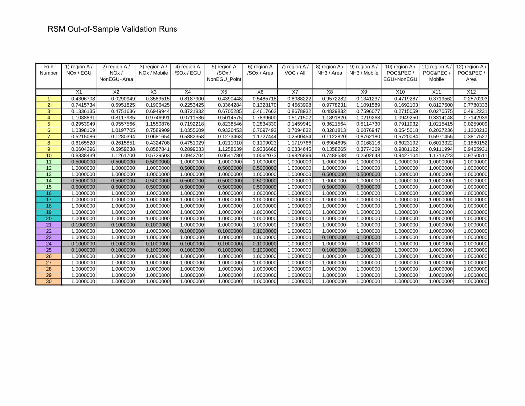
Run Number


2) region A / NOx /

NonEGU+Area



5) region A /SOx /

NonEGU_Point






EGU+NonEGU


Mobile


Area

X1 X2 X3 X4 X5 X6 X7 X8 X9 X10 X11 X121 0.4306708 0.0290949 0.3589515 0.8187900 0.4390448 0.5485718 0.8088222 0.9572282 0.1341237 0.4719287 0.3719562 0.25702032 0.7415734 0.6951825 0.1906425 0.2253425 0.3364284 0.1328170 0.4563998 0.9778231 1.1091589 0.1692103 0.8127500 0.77803333 0.1336135 0.4751636 0.6949944 0.8721832 0.6705285 0.4617662 0.8678932 0.4829832 0.7596077 0.2715059 0.0270575 0.49122314 1.1088831 0.8117935 0.9746991 0.0711536 0.5014575 0.7839600 0.5171502 1.1891820 1.0219268 1.0949250 0.3314148 0.71429395 0.2953949 0.9557566 1.1550876 0.7192218 0.8238546 0.2834330 0.1459941 0.3621564 0.5114730 0.7911932 1.0215415 0.02590096 1.0398169 1.0197705 0.7589909 1.0355609 0.9326453 0.7097492 0.7094832 0.3281813 0.6076947 0.0545018 0.2027236 1.12002127 0.5215086 0.1280394 0.0681654 0.5882358 0.1273463 1.1727444 0.2500454 0.1122820 0.8762180 0.5720084 0.5971455 0.38175278 0.6165520 0.2615851 0.4324708 0.4751029 1.0211010 0.1109023 1.1719766 0.6904895 0.0168116 0.6023192 0.6013322 0.18801529 0.0604296 0.5959238 0.8587841 0.2899033 1.1258639 0.9336668 0.0834645 0.1358265 0.3774369 0.9881122 0.9111994 0.946593110 0.8838439 1.1261700 0.5729503 1.0942704 0.0641780 1.0062073 0.9826899 0.7488538 0.2502648 0.9427104 1.1713723 0.975051111 0.5000000 0.5000000 0.5000000 1.0000000 1.0000000 1.0000000 1.0000000 1.0000000 1.0000000 1.0000000 1.0000000 1.000000012 1.0000000 1.0000000 1.0000000 0.5000000 0.5000000 0.5000000 1.0000000 1.0000000 1.0000000 1.0000000 1.0000000 1.000000013 1.0000000 1.0000000 1.0000000 1.0000000 1.0000000 1.0000000 1.0000000 0.5000000 0.5000000 1.0000000 1.0000000 1.000000014 0.5000000 0.5000000 0.5000000 0.5000000 0.5000000 0.5000000 1.0000000 1.0000000 1.0000000 1.0000000 1.0000000 1.000000015 0.5000000 0.5000000 0.5000000 0.5000000 0.5000000 0.5000000 1.0000000 0.5000000 0.5000000 1.0000000 1.0000000 1.000000016 1.0000000 1.0000000 1.0000000 1.0000000 1.0000000 1.0000000 1.0000000 1.0000000 1.0000000 1.0000000 1.0000000 1.000000017 1.0000000 1.0000000 1.0000000 1.0000000 1.0000000 1.0000000 1.0000000 1.0000000 1.0000000 1.0000000 1.0000000 1.000000018 1.0000000 1.0000000 1.0000000 1.0000000 1.0000000 1.0000000 1.0000000 1.0000000 1.0000000 1.0000000 1.0000000 1.000000019 1.0000000 1.0000000 1.0000000 1.0000000 1.0000000 1.0000000 1.0000000 1.0000000 1.0000000 1.0000000 1.0000000 1.000000020 1.0000000 1.0000000 1.0000000 1.0000000 1.0000000 1.0000000 1.0000000 1.0000000 1.0000000 1.0000000 1.0000000 1.000000021 0.1000000 0.1000000 0.1000000 1.0000000 1.0000000 1.0000000 1.0000000 1.0000000 1.0000000 1.0000000 1.0000000 1.000000022 1.0000000 1.0000000 1.0000000 0.1000000 0.1000000 0.1000000 1.0000000 1.0000000 1.0000000 1.0000000 1.0000000 1.000000023 1.0000000 1.0000000 1.0000000 1.0000000 1.0000000 1.0000000 1.0000000 0.1000000 0.1000000 1.0000000 1.0000000 1.000000024 0.1000000 0.1000000 0.1000000 0.1000000 0.1000000 0.1000000 1.0000000 1.0000000 1.0000000 1.0000000 1.0000000 1.000000025 0.1000000 0.1000000 0.1000000 0.1000000 0.1000000 0.1000000 1.0000000 0.1000000 0.1000000 1.0000000 1.0000000 1.000000026 1.0000000 1.0000000 1.0000000 1.0000000 1.0000000 1.0000000 1.0000000 1.0000000 1.0000000 1.0000000 1.0000000 1.000000027 1.0000000 1.0000000 1.0000000 1.0000000 1.0000000 1.0000000 1.0000000 1.0000000 1.0000000 1.0000000 1.0000000 1.000000028 1.0000000 1.0000000 1.0000000 1.0000000 1.0000000 1.0000000 1.0000000 1.0000000 1.0000000 1.0000000 1.0000000 1.000000029 1.0000000 1.0000000 1.0000000 1.0000000 1.0000000 1.0000000 1.0000000 1.0000000 1.0000000 1.0000000 1.0000000 1.000000030 1.0000000 1.0000000 1.0000000 1.0000000 1.0000000 1.0000000 1.0000000 1.0000000 1.0000000 1.0000000 1.0000000 1.0000000

RSM Out-of-Sample Validation Runs

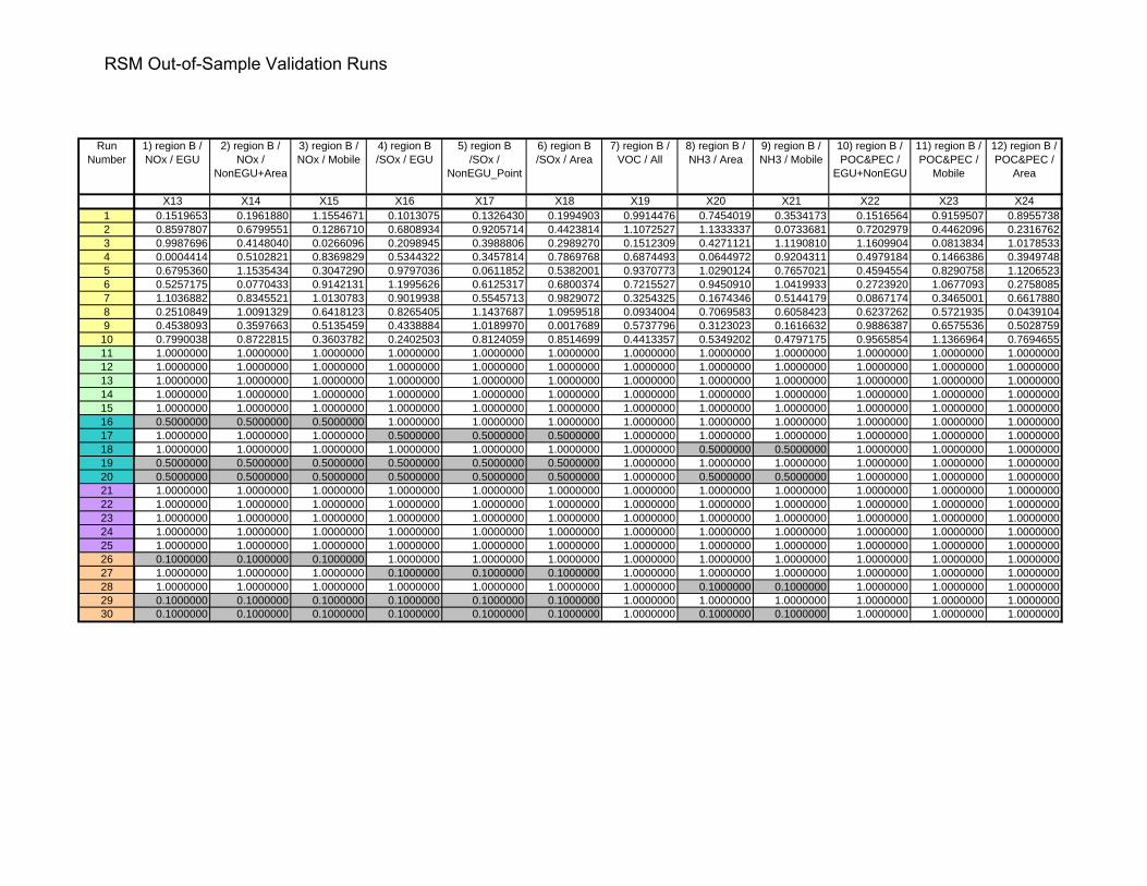
Run Number

123456789101112131415161718192021222324252627282930


2) region B / NOx /

NonEGU+Area



5) region B /SOx /

NonEGU_Point






EGU+NonEGU


Mobile


Area

X13 X14 X15 X16 X17 X18 X19 X20 X21 X22 X23 X240.1519653 0.1961880 1.1554671 0.1013075 0.1326430 0.1994903 0.9914476 0.7454019 0.3534173 0.1516564 0.9159507 0.89557380.8597807 0.6799551 0.1286710 0.6808934 0.9205714 0.4423814 1.1072527 1.1333337 0.0733681 0.7202979 0.4462096 0.23167620.9987696 0.4148040 0.0266096 0.2098945 0.3988806 0.2989270 0.1512309 0.4271121 1.1190810 1.1609904 0.0813834 1.01785330.0004414 0.5102821 0.8369829 0.5344322 0.3457814 0.7869768 0.6874493 0.0644972 0.9204311 0.4979184 0.1466386 0.39497480.6795360 1.1535434 0.3047290 0.9797036 0.0611852 0.5382001 0.9370773 1.0290124 0.7657021 0.4594554 0.8290758 1.12065230.5257175 0.0770433 0.9142131 1.1995626 0.6125317 0.6800374 0.7215527 0.9450910 1.0419933 0.2723920 1.0677093 0.27580851.1036882 0.8345521 1.0130783 0.9019938 0.5545713 0.9829072 0.3254325 0.1674346 0.5144179 0.0867174 0.3465001 0.66178800.2510849 1.0091329 0.6418123 0.8265405 1.1437687 1.0959518 0.0934004 0.7069583 0.6058423 0.6237262 0.5721935 0.04391040.4538093 0.3597663 0.5135459 0.4338884 1.0189970 0.0017689 0.5737796 0.3123023 0.1616632 0.9886387 0.6575536 0.50287590.7990038 0.8722815 0.3603782 0.2402503 0.8124059 0.8514699 0.4413357 0.5349202 0.4797175 0.9565854 1.1366964 0.76946551.0000000 1.0000000 1.0000000 1.0000000 1.0000000 1.0000000 1.0000000 1.0000000 1.0000000 1.0000000 1.0000000 1.00000001.0000000 1.0000000 1.0000000 1.0000000 1.0000000 1.0000000 1.0000000 1.0000000 1.0000000 1.0000000 1.0000000 1.00000001.0000000 1.0000000 1.0000000 1.0000000 1.0000000 1.0000000 1.0000000 1.0000000 1.0000000 1.0000000 1.0000000 1.00000001.0000000 1.0000000 1.0000000 1.0000000 1.0000000 1.0000000 1.0000000 1.0000000 1.0000000 1.0000000 1.0000000 1.00000001.0000000 1.0000000 1.0000000 1.0000000 1.0000000 1.0000000 1.0000000 1.0000000 1.0000000 1.0000000 1.0000000 1.00000000.5000000 0.5000000 0.5000000 1.0000000 1.0000000 1.0000000 1.0000000 1.0000000 1.0000000 1.0000000 1.0000000 1.00000001.0000000 1.0000000 1.0000000 0.5000000 0.5000000 0.5000000 1.0000000 1.0000000 1.0000000 1.0000000 1.0000000 1.00000001.0000000 1.0000000 1.0000000 1.0000000 1.0000000 1.0000000 1.0000000 0.5000000 0.5000000 1.0000000 1.0000000 1.00000000.5000000 0.5000000 0.5000000 0.5000000 0.5000000 0.5000000 1.0000000 1.0000000 1.0000000 1.0000000 1.0000000 1.00000000.5000000 0.5000000 0.5000000 0.5000000 0.5000000 0.5000000 1.0000000 0.5000000 0.5000000 1.0000000 1.0000000 1.00000001.0000000 1.0000000 1.0000000 1.0000000 1.0000000 1.0000000 1.0000000 1.0000000 1.0000000 1.0000000 1.0000000 1.00000001.0000000 1.0000000 1.0000000 1.0000000 1.0000000 1.0000000 1.0000000 1.0000000 1.0000000 1.0000000 1.0000000 1.00000001.0000000 1.0000000 1.0000000 1.0000000 1.0000000 1.0000000 1.0000000 1.0000000 1.0000000 1.0000000 1.0000000 1.00000001.0000000 1.0000000 1.0000000 1.0000000 1.0000000 1.0000000 1.0000000 1.0000000 1.0000000 1.0000000 1.0000000 1.00000001.0000000 1.0000000 1.0000000 1.0000000 1.0000000 1.0000000 1.0000000 1.0000000 1.0000000 1.0000000 1.0000000 1.00000000.1000000 0.1000000 0.1000000 1.0000000 1.0000000 1.0000000 1.0000000 1.0000000 1.0000000 1.0000000 1.0000000 1.00000001.0000000 1.0000000 1.0000000 0.1000000 0.1000000 0.1000000 1.0000000 1.0000000 1.0000000 1.0000000 1.0000000 1.00000001.0000000 1.0000000 1.0000000 1.0000000 1.0000000 1.0000000 1.0000000 0.1000000 0.1000000 1.0000000 1.0000000 1.00000000.1000000 0.1000000 0.1000000 0.1000000 0.1000000 0.1000000 1.0000000 1.0000000 1.0000000 1.0000000 1.0000000 1.00000000.1000000 0.1000000 0.1000000 0.1000000 0.1000000 0.1000000 1.0000000 0.1000000 0.1000000 1.0000000 1.0000000 1.0000000

RSM Out-of-Sample Validation Runs

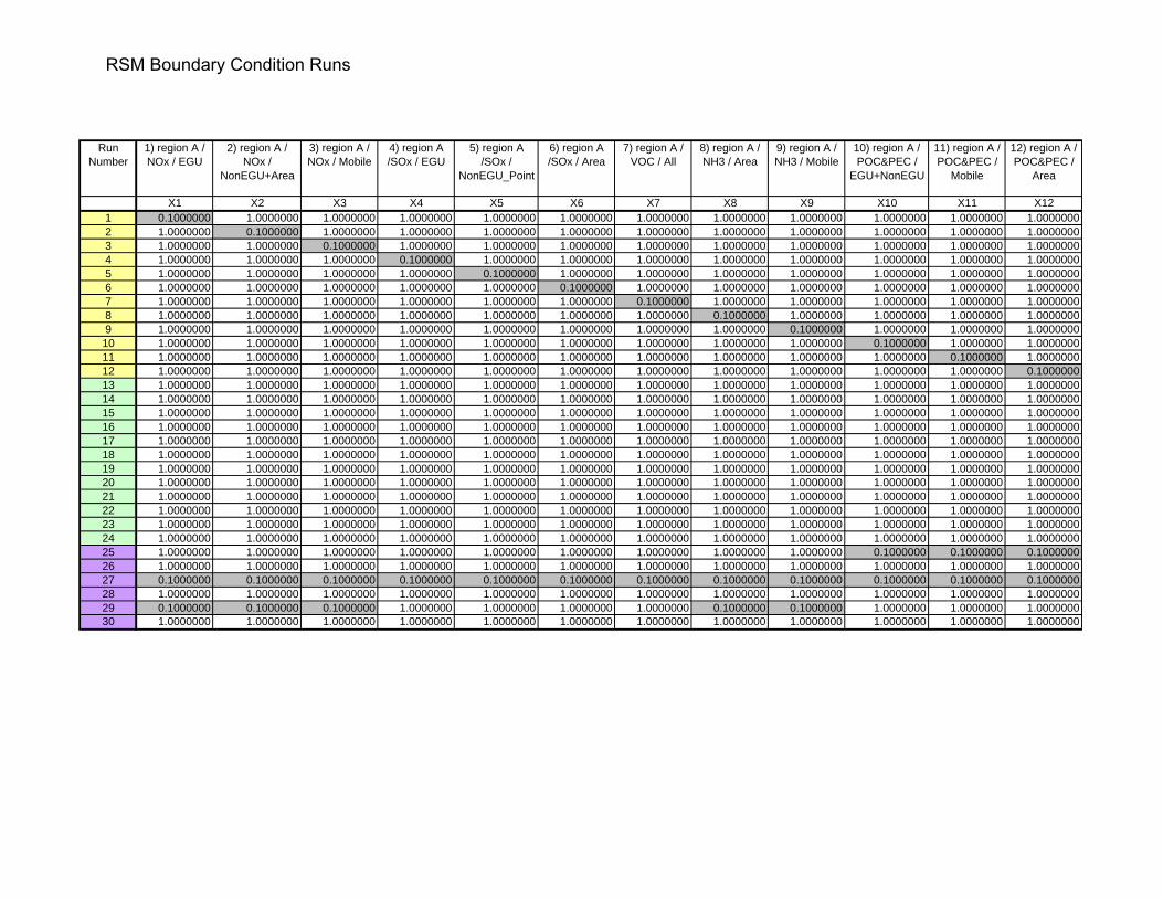
Run Number


2) region A / NOx /

NonEGU+Area



5) region A /SOx /

NonEGU_Point






EGU+NonEGU


Mobile


Area

X1 X2 X3 X4 X5 X6 X7 X8 X9 X10 X11 X121 0.1000000 1.0000000 1.0000000 1.0000000 1.0000000 1.0000000 1.0000000 1.0000000 1.0000000 1.0000000 1.0000000 1.00000002 1.0000000 0.1000000 1.0000000 1.0000000 1.0000000 1.0000000 1.0000000 1.0000000 1.0000000 1.0000000 1.0000000 1.00000003 1.0000000 1.0000000 0.1000000 1.0000000 1.0000000 1.0000000 1.0000000 1.0000000 1.0000000 1.0000000 1.0000000 1.00000004 1.0000000 1.0000000 1.0000000 0.1000000 1.0000000 1.0000000 1.0000000 1.0000000 1.0000000 1.0000000 1.0000000 1.00000005 1.0000000 1.0000000 1.0000000 1.0000000 0.1000000 1.0000000 1.0000000 1.0000000 1.0000000 1.0000000 1.0000000 1.00000006 1.0000000 1.0000000 1.0000000 1.0000000 1.0000000 0.1000000 1.0000000 1.0000000 1.0000000 1.0000000 1.0000000 1.00000007 1.0000000 1.0000000 1.0000000 1.0000000 1.0000000 1.0000000 0.1000000 1.0000000 1.0000000 1.0000000 1.0000000 1.00000008 1.0000000 1.0000000 1.0000000 1.0000000 1.0000000 1.0000000 1.0000000 0.1000000 1.0000000 1.0000000 1.0000000 1.00000009 1.0000000 1.0000000 1.0000000 1.0000000 1.0000000 1.0000000 1.0000000 1.0000000 0.1000000 1.0000000 1.0000000 1.000000010 1.0000000 1.0000000 1.0000000 1.0000000 1.0000000 1.0000000 1.0000000 1.0000000 1.0000000 0.1000000 1.0000000 1.000000011 1.0000000 1.0000000 1.0000000 1.0000000 1.0000000 1.0000000 1.0000000 1.0000000 1.0000000 1.0000000 0.1000000 1.000000012 1.0000000 1.0000000 1.0000000 1.0000000 1.0000000 1.0000000 1.0000000 1.0000000 1.0000000 1.0000000 1.0000000 0.100000013 1.0000000 1.0000000 1.0000000 1.0000000 1.0000000 1.0000000 1.0000000 1.0000000 1.0000000 1.0000000 1.0000000 1.000000014 1.0000000 1.0000000 1.0000000 1.0000000 1.0000000 1.0000000 1.0000000 1.0000000 1.0000000 1.0000000 1.0000000 1.000000015 1.0000000 1.0000000 1.0000000 1.0000000 1.0000000 1.0000000 1.0000000 1.0000000 1.0000000 1.0000000 1.0000000 1.000000016 1.0000000 1.0000000 1.0000000 1.0000000 1.0000000 1.0000000 1.0000000 1.0000000 1.0000000 1.0000000 1.0000000 1.000000017 1.0000000 1.0000000 1.0000000 1.0000000 1.0000000 1.0000000 1.0000000 1.0000000 1.0000000 1.0000000 1.0000000 1.000000018 1.0000000 1.0000000 1.0000000 1.0000000 1.0000000 1.0000000 1.0000000 1.0000000 1.0000000 1.0000000 1.0000000 1.000000019 1.0000000 1.0000000 1.0000000 1.0000000 1.0000000 1.0000000 1.0000000 1.0000000 1.0000000 1.0000000 1.0000000 1.000000020 1.0000000 1.0000000 1.0000000 1.0000000 1.0000000 1.0000000 1.0000000 1.0000000 1.0000000 1.0000000 1.0000000 1.000000021 1.0000000 1.0000000 1.0000000 1.0000000 1.0000000 1.0000000 1.0000000 1.0000000 1.0000000 1.0000000 1.0000000 1.000000022 1.0000000 1.0000000 1.0000000 1.0000000 1.0000000 1.0000000 1.0000000 1.0000000 1.0000000 1.0000000 1.0000000 1.000000023 1.0000000 1.0000000 1.0000000 1.0000000 1.0000000 1.0000000 1.0000000 1.0000000 1.0000000 1.0000000 1.0000000 1.000000024 1.0000000 1.0000000 1.0000000 1.0000000 1.0000000 1.0000000 1.0000000 1.0000000 1.0000000 1.0000000 1.0000000 1.000000025 1.0000000 1.0000000 1.0000000 1.0000000 1.0000000 1.0000000 1.0000000 1.0000000 1.0000000 0.1000000 0.1000000 0.100000026 1.0000000 1.0000000 1.0000000 1.0000000 1.0000000 1.0000000 1.0000000 1.0000000 1.0000000 1.0000000 1.0000000 1.000000027 0.1000000 0.1000000 0.1000000 0.1000000 0.1000000 0.1000000 0.1000000 0.1000000 0.1000000 0.1000000 0.1000000 0.100000028 1.0000000 1.0000000 1.0000000 1.0000000 1.0000000 1.0000000 1.0000000 1.0000000 1.0000000 1.0000000 1.0000000 1.000000029 0.1000000 0.1000000 0.1000000 1.0000000 1.0000000 1.0000000 1.0000000 0.1000000 0.1000000 1.0000000 1.0000000 1.000000030 1.0000000 1.0000000 1.0000000 1.0000000 1.0000000 1.0000000 1.0000000 1.0000000 1.0000000 1.0000000 1.0000000 1.0000000

RSM Boundary Condition Runs

Run Number

123456789101112131415161718192021222324252627282930


2) region B / NOx /

NonEGU+Area



5) region B /SOx /

NonEGU_Point






EGU+NonEGU


Mobile


Area

X13 X14 X15 X16 X17 X18 X19 X20 X21 X22 X23 X241.0000000 1.0000000 1.0000000 1.0000000 1.0000000 1.0000000 1.0000000 1.0000000 1.0000000 1.0000000 1.0000000 1.00000001.0000000 1.0000000 1.0000000 1.0000000 1.0000000 1.0000000 1.0000000 1.0000000 1.0000000 1.0000000 1.0000000 1.00000001.0000000 1.0000000 1.0000000 1.0000000 1.0000000 1.0000000 1.0000000 1.0000000 1.0000000 1.0000000 1.0000000 1.00000001.0000000 1.0000000 1.0000000 1.0000000 1.0000000 1.0000000 1.0000000 1.0000000 1.0000000 1.0000000 1.0000000 1.00000001.0000000 1.0000000 1.0000000 1.0000000 1.0000000 1.0000000 1.0000000 1.0000000 1.0000000 1.0000000 1.0000000 1.00000001.0000000 1.0000000 1.0000000 1.0000000 1.0000000 1.0000000 1.0000000 1.0000000 1.0000000 1.0000000 1.0000000 1.00000001.0000000 1.0000000 1.0000000 1.0000000 1.0000000 1.0000000 1.0000000 1.0000000 1.0000000 1.0000000 1.0000000 1.00000001.0000000 1.0000000 1.0000000 1.0000000 1.0000000 1.0000000 1.0000000 1.0000000 1.0000000 1.0000000 1.0000000 1.00000001.0000000 1.0000000 1.0000000 1.0000000 1.0000000 1.0000000 1.0000000 1.0000000 1.0000000 1.0000000 1.0000000 1.00000001.0000000 1.0000000 1.0000000 1.0000000 1.0000000 1.0000000 1.0000000 1.0000000 1.0000000 1.0000000 1.0000000 1.00000001.0000000 1.0000000 1.0000000 1.0000000 1.0000000 1.0000000 1.0000000 1.0000000 1.0000000 1.0000000 1.0000000 1.00000001.0000000 1.0000000 1.0000000 1.0000000 1.0000000 1.0000000 1.0000000 1.0000000 1.0000000 1.0000000 1.0000000 1.00000000.1000000 1.0000000 1.0000000 1.0000000 1.0000000 1.0000000 1.0000000 1.0000000 1.0000000 1.0000000 1.0000000 1.00000001.0000000 0.1000000 1.0000000 1.0000000 1.0000000 1.0000000 1.0000000 1.0000000 1.0000000 1.0000000 1.0000000 1.00000001.0000000 1.0000000 0.1000000 1.0000000 1.0000000 1.0000000 1.0000000 1.0000000 1.0000000 1.0000000 1.0000000 1.00000001.0000000 1.0000000 1.0000000 0.1000000 1.0000000 1.0000000 1.0000000 1.0000000 1.0000000 1.0000000 1.0000000 1.00000001.0000000 1.0000000 1.0000000 1.0000000 0.1000000 1.0000000 1.0000000 1.0000000 1.0000000 1.0000000 1.0000000 1.00000001.0000000 1.0000000 1.0000000 1.0000000 1.0000000 0.1000000 1.0000000 1.0000000 1.0000000 1.0000000 1.0000000 1.00000001.0000000 1.0000000 1.0000000 1.0000000 1.0000000 1.0000000 0.1000000 1.0000000 1.0000000 1.0000000 1.0000000 1.00000001.0000000 1.0000000 1.0000000 1.0000000 1.0000000 1.0000000 1.0000000 0.1000000 1.0000000 1.0000000 1.0000000 1.00000001.0000000 1.0000000 1.0000000 1.0000000 1.0000000 1.0000000 1.0000000 1.0000000 0.1000000 1.0000000 1.0000000 1.00000001.0000000 1.0000000 1.0000000 1.0000000 1.0000000 1.0000000 1.0000000 1.0000000 1.0000000 0.1000000 1.0000000 1.00000001.0000000 1.0000000 1.0000000 1.0000000 1.0000000 1.0000000 1.0000000 1.0000000 1.0000000 1.0000000 0.1000000 1.00000001.0000000 1.0000000 1.0000000 1.0000000 1.0000000 1.0000000 1.0000000 1.0000000 1.0000000 1.0000000 1.0000000 0.10000001.0000000 1.0000000 1.0000000 1.0000000 1.0000000 1.0000000 1.0000000 1.0000000 1.0000000 1.0000000 1.0000000 1.00000001.0000000 1.0000000 1.0000000 1.0000000 1.0000000 1.0000000 1.0000000 1.0000000 1.0000000 0.1000000 0.1000000 0.10000001.0000000 1.0000000 1.0000000 1.0000000 1.0000000 1.0000000 1.0000000 1.0000000 1.0000000 1.0000000 1.0000000 1.00000000.1000000 0.1000000 0.1000000 0.1000000 0.1000000 0.1000000 0.1000000 0.1000000 0.1000000 0.1000000 0.1000000 0.10000001.0000000 1.0000000 1.0000000 1.0000000 1.0000000 1.0000000 1.0000000 1.0000000 1.0000000 1.0000000 1.0000000 1.00000000.1000000 0.1000000 0.1000000 1.0000000 1.0000000 1.0000000 1.0000000 0.1000000 0.1000000 1.0000000 1.0000000 1.0000000

RSM Boundary Condition Runs

technical support document for the proposed pm … support document for the proposed pm naaqs rule...

Documents