technicalmemorandum83997 interactive -uigitansignal processor
TRANSCRIPT
...... I/ (._,+_," i
, TechnicalMemorandum83997
-i i" "Interactive u g tanSignal Processor
(_ASA-_/_-83997) ZNTE.;ACIIVE _/GJ[TAL SIGNAL _184-3q9714
: PaOCESSO_ (blASA} ltJ7 p HE A(,8/MY A01CSCi 09B
" " Uaclas -
- - G3/61 2.]127
W. H. Mish, R. M. Wenger, K. W. Behannon,
and J. B. Byrnes _:
I1 SEPTEMBER1982 __ '-'_
(Revised Moy 1984' //_.._;_j_;_:%E_",.'_'",."_. _ ,_ _ r-_
NationalAeronauticsand V_.! !"_._SpaceAdministration ",_ _m'r,_1¢_," ,%
Goddard Space Flight Center
Greenbelt.Maryland20771
1984026903
' INTERACTIVE DIGITAL SIGNAL PROCESSOR
by
William H. Mish
Laboratory for Extraterrestrial Physics
NASA/Goddard Space Flight Center
Greenbelt, Maryland 20771
Ray M. Wenger
Computer Science Corporation8728 Colesville Rd
_ Silver Spring, Maryland 20910
Kenneth W. Behannon
Laboratory for Extraterrestrial PhysicsNASAIGoddard Space Flight Center
Greenbelt, Maryland 20771
James B. Byrnes
Laboratory for Extraterrestrial PhysicsNASA/Goddard Space __ight Center
Greenbelt, Maryland 20771I
IP
4
September 1982
Revised May 1984
1984026903-002
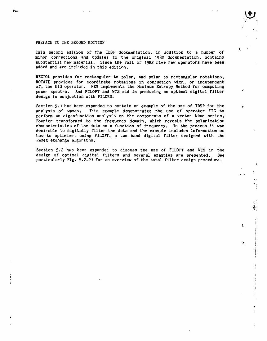
PREFACE TO THE SECOND EDITION
This second edition of the IDSP documentation, in addition to a number of
minor corrections and updates to the original 1982 documentation, contains
substantial new material. Since the Fall of 1982 five new operators have beenadded and are included in this edition.
RECPOL provides for rectangular to polar, and polar to rectangular rotations,
ROTATE provides for coordinate rotations in conJuction with, or independentof, the EIG operator. MEM implements the Maximum Entropy Method for computing
power spectra. And FILOPT and WTS aid in producing an optimal digital filter
design in conJuction with FILDES.
Section 5.1 has been expanded to contain an example of the use of IDSP for the ,
analysis of waves. This example demonstrates the use of operator EIG to
perform an eigenfunction analysis on the components of a vector time series,
Fourier transformed to the frequency domain, which reveals the polarization
characteristics of the data as a function of frequency. In the process it wasdesirable to digitally filter the data and the example includes information on
how to optimize, using FILOPT, a two band digital filter designed with theRemez exchange algorithm.
Section 5.2 has been expanded to discuss the use of FILOPT and WTS in the
design of optimal digital filters and several examples are presented. Seeparticularly Fig. 5.2-21 for an overview of the total filter design procedure.
1984026903-003

ABSTRACT
The Interactive Digital Signal Processor (IDSP) is implemented on a VAX11/780 under VMS. It consists of a set of time series analysis "Operators"
each of which operates on an input file to produce an output file; theoperators can be executed in any order that makes sense and recursively, if
desired. The operators are the various algorltl_s that have been used in
digital time series analysis work over the years. In addition, there is
provision for user written operators to be easily interfaced to the system.
• The system can be operated both interactively and in batch mode.
In IDSP a file can consist of up to n (currently n=8) simultaneous time
, series. Thus storage for a file can be subdivided such that it is used, for
example, entirely for one long single time series or for as many as n shortertime series, such as the components of a vector. An operator always operates
simultaneously on all of the time series in a file.
IDSP currently includes over thirty standard operators that range from Fourier
transform operations (FFT,FFTIN,WINDOW,SPECT), design and application of
digital filters (FILDES, FILOPT,FILTER,WTS), elgenvalue analysis (EIG), to
operators that provide graphical output (GRAPH,GRAFCK), allow batch operation
(REDO), editing (CONCAT, EDHIST, EDIT,INTERP, SUBSET,SUBSER) and displayinformation (SHOW, CMDHIS). The complete set of standard operators is listedbelow.
AVER, CMDHIS, CONCAT, COPY, IX:L, DSTAT, EDHIST, EDIT, EIG, FILDES, FILOPT,
FILTER, FFT, FFTIN, FLOP, GRAFCK, GRAPH, INTERP, MEM, MNFLD, NORM, RECPOL,
REDO, ROTATE, SETUP, SHOW, SPECT, SUBSER, SUBSET, TRACE, WINDOW, WTS, STOP.
IDSP is being used extensively to process data sets obtained from scientific
experiments onboard spacecraft such as Dynamics Explorer, ISEE, IMP andVoyager. In addition IDSP provides an excellent teaching tool for
demonstrating the application of the various time series operators toartiflcally-generated signals.
IDSP is available from the Computer Software Management and Information Center
l (COSMIC), 112 Barrow HaI_, University of Georgia, Athens, Georgia 30602,Program Number GSC-12862. I
i
i
abstract 5/29/8L1
1984026903-004

TABLE OF CONTENTS
lo0) INTRODUCTION OF IDSP ......................................... Ie0--I
2.0) AN EXAMPLE OF THE USE OF IDSP................................ 2.0-I
3 O) OVERVIEW OF THE IDSP SYSTB' DESIGN 3 0 Il .alllOlelml.lllell.ll'llOll l
4.0) HOW TO START USING IDSP ...................................... 4.0-I
5.0) APPLICATION NOTES
5.1) FOURIER TRANSFORM, SPECTRAL MATRICES, EIGENVECTOR COORDINATES,
MAXMIU/4 ENTROPY METHOD (OPERATORS FFT, SPECT, EIG and MEN).. 5.1-I|
5.I.I) OPERATOR FFT .......................................... 5. I-I
5.1.2) OPERATOR SPECT ........................................ 5.1-5
5.1.3) STATISTICAL STABILITY ................................. 5.1-95.1.4) OPERATOR EIG .......................................... 5.1-10
5.1.5) EXAMPLE: THE USE OF IDSP IN THE ANALYSIS OF WAVES IN
DEEP SPACE DATA ....................................... 5.1-I?
5.1.6) OPERATOR MEM .......................................... 5.1-23
5.2) DIGITAL FILTERS (OPERATORS FILDES,FILOPT, FILTER and WTS) .... 5.2-I
5.2.1) INTRODUCTION TO DIGITAL FILTER DESIGN USING REMEZ
_ EXCHANGE . . .5.2.2)DESIGN 52-i• • . 5.2-2
5.2.3) USE OF A DIFFERENTIATING FILTER ....................... 5.2-8
5.3) THE EFFECT OF WINDOWING, ZERO PADDING AND OBSERVATIONTIME ON ESTIMATION OF SPECTRA OF SINUSOIDS
(OPERATORS SETUP, WINDOW, FFT and SPECT) ..................... 5.3-I t
6.0) IDSP OPERATOR DESCRIPTIONS '!
6.1) AVER_average every n points ............................... 6.1-I
¢ 6.2) CMDHIS--listing of commands issued during current session 6.2-I {P
6.3) CONCAT--concatenate two different datasets ................. 6.3-I
6.4) COPY_copy one dataset to another .......................... 6.4-I
6.5) DCL_allow user to enter VAX DCL commands .................. 6.5-I
6.6) DSTAT_compute dataset statistics .......................... 6.6-I
6.7) EDHIST_alIow user to edit history of dataset .............. 6.7-I
6.8) EDIT--Dlsplay series and Intersctlvely edit on a HP264BA \Graphics terminal .......................................... 6.8-1
ii !1
table of contents 5/29/84
1984026903-005
-/
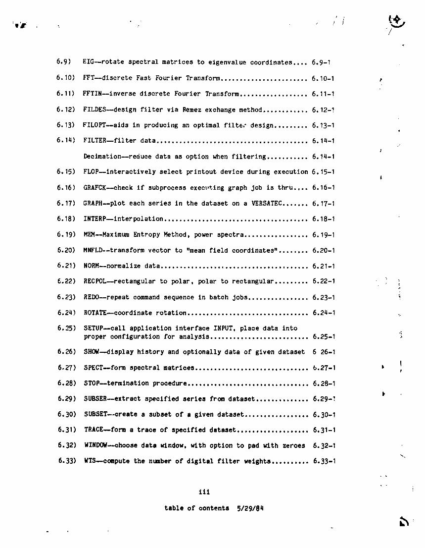
6.9) ElO--rotate spectral matrices to eigenvalue coordinates.... 6.9-I
5.10) FFT--discrete Fast Fourier Transform.......................6.10-I
6.11) FFTIN--Inverse discrete Fourier Transform..................6.11-I
6.12) FILDES--deslgn filter via Remez exchange method............ 6.12-!
6.13) FILOPT_aids in producing an optimal lilts,-design......... 6.13-I#
6.14) FILTER--filter data........................................6.14-I/
]
Decimation--reducedata as option when filtering........... 6.14-I
6.15) FLOP--interactively select printout device during execution 6.15-IJ
6.16) GRAFCK--check If subprocess exect,tlnggraph Job is thru.... 6.16-I
6.17) GRAPH_pZot each series in the dataset on a VERSATEC....... 6.17-I
6.18) INTERP--interpolatlon......................................6.18-I
6.19) MEM--Maxlmum Entropy Method, power spectra.................6.19-I
6.20) MNFLD--transform vector to "mean field coordinates"........ 6.20-I
6.21) NORM--normallze data.......................................6.21-I
6.22) RECPOL--rectangular to polar, polar'to rectangular......... 6.22-I ,' ;A
6.23) REDO--repeat command sequence in batch Jobs................6.23-I
6.24) ROTATE--coordlnaterotation................................6.24-I
6.25) SETUPNcall application interface INPUT, place data intoproper configuration for analysis..........................6.25-I
6.26) SHOW--display history and optionally data of given dataset 6 26-I
6_27) SPECTNform spectral matrices..............................b.27-I m I?
6.28) STOP_termlnatlon procedure................................6.28-I
6.29) SUBSER--extract specified series from dataset.............. 6.29-I
6.30) St_SET--create a 3ubset of a given dataset.................6.30-I
6.31) TRACE_form a trace of specified dataaet ................... 6.31-1
6.32) WINDOW_vhooae data window, with option to pad with zeroes 6.32-1
6.33) WTS--compute the number of dtgltal filter weights .......... 6.33-1
itl
table of contents 5/29/84
1984026903-006

ACKNOWLEDGEMENTS
BIBLIOGRAPHY
APPENDIX A-WRITING INPUT ROUTINES FOR IDSP.............................. A-I
APPENDIX B-WRITING USER DEFINED OPERATORS FOR IDSP...................... B-I
APPENDIX C-DESIGN CONSIDERATIONS FOR IDSP............................... C-I
APPENDIX D-EXECUTION OF BATCH JOBS...................................... D-I
APPENDIX E-CONVENTIONS ON DATASET NAMES................................. E-I
i APPENDIX F-EXISTING INPUT ROUTINES...................................... F-I
APPENDIX G-CHANGES INCORPORATED INTO VERSION I OF IDSP.................. G-I
APPENDIX H-EXISTING USER OPERATORS...................................... H-I
APPENDIX I-INSTALLATION PROCEDURE....................................... I-I
APPENDIX J-AN INPUT ROUTINE FOR GENERATION OF FEST DATA................. J-1
R
b_
iv
, table or" oontents 5/29/8_ 'i
/
1984026903-007

LIST OF TABLES
Table 2.0-1 Page 2.0-2 /Part of the output from the FILDES operator that gives a listing of the filter
coefficients and other related parameters for the 5 band filter shown in Fig.2.0-3.
Table 5.1-1 Page 5.1-15Polarization parameters for operator EIG
Table 5.2-I Page 5.2-10 •
Part of the output from the FILDES operator that gives a listing of the filter
coefficients and other related parameters for the 3 band filter shown in Fig.5.2-5.
oTable 5.2-2 Page 5.2-11
Part of the output from _he FILDES operator that gives a listing of the filtercoefficients and other related parameters for the differentiating filter shown
in Fig. 5.2-17.
Table 5.3-1 Page 5.3-1Criteria for the selection of a "window" function.
L
IP
v
list of tables 5/31/84
lip
1984026903-008

LIST OF FIGURES
Fig.l.0-1 Page 1.0-qA schematic of mapping an analog phenomenon to the digital world.
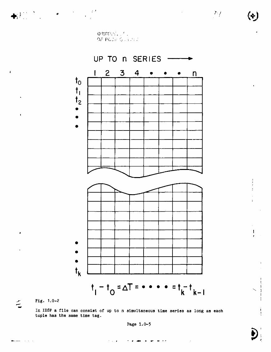
Fig. 1.0-2 Page 1.0-5In IDSP a file can consist of up to n simultaneous time series as long as each
tuple has the same time tag.
Fig. 1.0-3 Page 1.0-6
IDSP processes the time serie_ according to two basic concepts: SPAN and
INTERVAL. The Interval is defined as the basic time segment to be analyzed--' the segment of data that is to be filtered or Fourier transfc,_ed, etc., by an
Operator. The Span is defined to be the total time under analysis-- composed
of one or more contiguous Intervals.
Fig. 2.0-I Page 2.0-3
On the Dynamics Explcrer Spacecraft there is a magnetic field experiment that
provides a vector measurement of the ambient magnetic field every 0.5 sac.
The data from one of the components of the vector is plotted as a function oftime.
Fig. 2.0-2 Page 2.0-3
Shows the spectrum resulting from application of Operators WINDOW, FFT, SPECT
and GRAPH on the time series from Fig. 2.0-I, note that at 0.0324 and 0.175 Hz
there are peaks in the spectrum resulting from the unwanted signals.
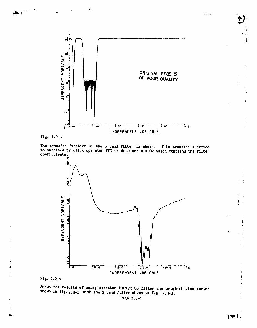
Fig. 2.0-3 Page 2.0-4The transfer function of the 5 band filter is shown. This transfer function
is obtained by using Operator FFT on data set WINDOW which contains the filtercoefficients.
Fig. 2. O-q Page 2.0-q
m Shows the results of using Operator FILTER to filter the original time series Ishown in Fig. 2.0-I with the 5 band filter shown in Fig. 2.0-3.
Fig. 5.1-1 Page 5.1-25This drawing is after Bergland, 1969 and shows what happens when a time seriesx(t) is Fourier transformed. X(J) is, in general, a complex series. The timeseries x(kAT) is assumed to be periodic in the time domain of period T. The
Fourier coefficients X(J£ O) are periodic over £. Each J should beinterpreted as a harmonic ndmber and each k a sampleS period number. Actual
frequency = Jfo" Actual time = kAT. When x(k) series is composed o£ realnumbers, as it-often is, the real part of X(J) is symmetric (even function)about the Nyquist frequency £f=£./2 and the imaginary part is antisymmeEric(odd function) about the Nyquts_c _equency. ,\
vl
list of flgures 5/29/8_
1984026903-009
,@j
Fig. 5.I-2 Page 5.1-26
Shows the real part of the results of Fourier transformin_ x(t) : 10 Cos
(2_*15*k*AT) + 5 Sin (2_*20*k*AT) sampled at 120 times per sec. Note that the
real part is symmetric about the Nyquist frequency, ff (i.e., BIN 120/2 = 60).
Fig. 5.I-3 Page 5.1-26
Shows the imaginary part of the results of Fourier transforming xrt) = 10 Cos
(2_*15*k*AT) + 5 S_.n (2T*20*k*AT) sampled at 120 times per sec. Note that the
imaginary part is antisymmetrlc about the Nyquist frequency, ff.
Fig. 5.1-4 Page 5.1-27
Shows the results of plotting the magnitude of the Fourier transform of x(t) -
10 Cos (2x*15*k*aT) + 5 Sin (2_*20*k*aT) sampled at 120 times per sac, which
shows the expected peaks at BINS 15 and 20, respectively and is symmetricabout the Nyqulst frequency.
Fig. 5.I-5 Page 5.1-27
A schematic of the operators FFT and SPECT and their associated data sets.
Flg. 5. I-6 Page 5.1-28
In the study of wave phenomena it is common to investlgate, using an
eigenfunction analysis, the fluctuations characteristics of the individualcomponents of the vector relative to the directional properties of the
fluctuation themselves. In such calculation the eigenvalues determine the
principal axes (o_2,o2_,as 2) of the characteristic variance (polarization)ellipse at each frequency estimate. The eigenvectors define the coordinatesystem corresponding to the directions of maximum (X), intermediate (Y) and
minimum (Z) oscillation in the wave at each frequency estimate. : :
Fig. 5.I-7 Page 5.1-29
Illustration of a plane, left-hand polarized wave, with front parallel to the ',
X-Y plane, shown at a succession of times t = 0 to t = 4 as it propagates inthe + Z direction (toward left). The perturbation vector b rotates CCW as
viewed frum upstream, its tlp describing the polarization ellipse in each 360°rotation. Although the total field B Is not shown, this case corresponds to
• _ positive and B negative. For right-handed waves propagating in the + Zdirection, the rotation sense would be CW. In the case shown, the spatialorientation of the ellipse remains constant during the tim,.- _nterval of thepropagation; in general, it may vary with time. _ l
P
Fig. 5.1-8 Page 5.1-30
A schematic of the operators EIG, SPECT, and DSTAT and the as_,iated data )sets.
Fig. 5.1-9 Page 5.1-31_aw vector magnetic field tlme series from the Voyager 2 spacecraft consisting
of 48-sac averages of field magnitude BH, and vector components XH, ¥H and Z.in hellographlc coordinates (ordinate "'units are nT -- nanotestras = I0"*-_
Gauss_ abscissa units used are sample number rather than time). The datacover a 24-hour period (1981/day 250) and show oscillation of field at twofrequencies differing by a factor of 20. Note that at the lower frequency
there are large amplitude variations In the field magnitude as well as in thecomponents.
vii
llst of figures 5/29/84
1984026903-010

Fig. 5.I-I0 Page 5.1-32
Power spectra for each time series shown in Fig. 5.I-9, plus the trace (Tr) of
the PS_ matrix (upper left, with field magnitude B spectrum). Ordinate unitsare nT=IHz and abscissa units are Hz. In each of the spectra a pronounccd
peak is seen centered on 1.75 X I0'm-4 Hz (dashed vertical llne) corresponding
to the low frequency, large amplitude variation prominent in the time ser_es.
This figure illustrates that there is relatively more power in d" nal
fluctuations than in magnitude (field strength) fluctuations.
Fig. 5.1-11 ' ",' -'J "• Eigenfunction properties of fluctuations shown in Fig. 5.1-9 over a _ , :_ a
range of frequency (q X I0*m-5 to q X !011-q Hz) that includes the p_.. _refrequency (delineated by the vertical hatched band). In the top panel the
trace spectrum is repeated from Fig. 5.1-10 for reference. Also shown, in
' panels 2 through q, respectively, are results from the application of EIG:degree of polarization, cosine of angle between _ and R, and wave elllptlcity(see text for discusslon).
Fig, 5, 1-12 Page 5,1-3qRaw time series of _4¢. 5.1-9 rotated into new coordinate system defined bythe wave eigenvector set, Operator EIG generates sets of eigenvalues andeigenvectors for each spectral estimate. Those determining the coordinates ofthe data in this figure corresponded to the estimate containing the spectral
peak denoted in Figs, 5.1-10 and 5,1-11, The XE direction is that of theelgenvector associated with the largest elgenvalue,-Z_ is that associated withthe smallest, and YE is that associated with the in%ermediate value. Sincethe wave is nearly circularly polarized, the amplitudes of the oscillations in
the YF direction are nearly as large as in the XR direction and essentiallyzero i-nthe Z_ direction. The magnitude of the field is not included since itis invarlant under rotation.
Fig. 5.1-13 Page 5.1-35Raw time series consisting of 9.6 seo averages for the portion of day 250 inwhich higher frequency fluctuations were seen also in Fig, 5,1-9 (1200-182qUT), Note that in this case the amplitude of variations in the magnetic field
magnitude (B H) is significantly lower than that of those in the vectorc_ponents.
, Fig. 5.1-14 Page 5.1-36The transfer function (frequency response) of the high pass filter designedwith operator FILDES to remove the low frequency oscillations from the rawdata, The function was obtained and plotted through the successive oporatorsiWINDOW FILDES, FFT WINDOW, and GRAPH FFTMP.
Fig. 5.1-15 Page 5.1-37Passband (PB) and Stopband (SB) ripple amplltvde as a function of relative
bandwelght WTX(1)/WTX(2) for a 125-coefflcient high pass filter with the givenbandedges. The vertical dashed llne delineates ripple characteristics
corresponding to relative weight value of 182 used for filter shown in Fig.
5.1-14 (see text and Fig. 5.1-16).
viii
list of figures 512918q
1984026903-011

ab,l_ • /,I ,
Fig. 5. I-16 Page 5.1-38Stopband minimum frequency response as a function of relative bandweight forfilter described in Fig. 5,1-15 caption, The second (right-handed) minimum atWTX(1)/WTX(2) = 182 is maximum attenuation state for the given configuration.
Fig. 5.1-17 Page 5.1-39Output from the application of the high pass filter to the time series shownin Fig. 5.1-13. The low frequency modulation of the data has been removedsuccessfully.
Fig. 5.1-1P Page 5.1-q0Power spectra for filtered time series shown in Fig. 5.1-17. Suppression ofpower in low frequency variations results in a more distinctive display of the"high" frequency shoulder, with peak less prominent in this case but centeredon a frequency of 3.4 X I0"*-3 Hz (dashed vertical, line).
a
Fig. 5.1-19 Page 5.1-41Elgenfunctlon properties of' the fluctuations shown in Fig. 5.1-17 in thefrequency band 0.001 to 0.01 Hz. Parameters plotted are same as those tn Fig.5.1-11. F-equency of peak power in the fluctuations is delineated by thevertical hatched band, Comparison with Fig. 5.1-11 shows properties of wavesat 3.4 X 10"*-3 Hz are similar to those of the 1.75 X 10"*-4 Hz waves.
Fig, 5.2-1 Page 5.2-12FIR filter design specifications after Schaff, 1979.
Fig. 5.2-2 Page 5.2-13
Raw magnetic field time series from the DE spacecraft sampled at twlce/sec,
showing contamination riding on top of the desired signal.
Fig. 5.2-3 Page 5.2-13
Power spectrum of the raw tlme series shown in Fig. 5.2-2 showing power at0.0324 and 0.175 Hz.
Fig. 5.2-4 Page 5.2-14 __le output of operator FILOPT showing 201o8(1 + deltal), and 20log(delta 2)plotted against the weight ratio, deltal/delta 2. From these plots weconcluded that the best tradeoff was a weight ratio of 2.5, which in turn was
used to design the filter shown in Fig. 5.2-5.
, Fig. 5.2-5 Page 5.2-15Transfer function of a notch filter designed to remove the unwanted 0.0324 Hz )signal from the original time series.
Fig. 5.2-6 Page 5.2-15Time series after applying the filter shown in Fig. 5.2-5.
_ Fig. 5.2-7 Page 5.2-16"i, Transfer function of a notch filter designed to remove the unwanted 0.175 Hza signal from the time series.
l-I
i
Ix
list of figures 5/29/8q
" m m m m=mm_ ; _ t
1984026903-012
I
!t
iJ
Flg. 5.2-8 Page 5.2-16" Time series after application of both the filter shown ir Flg. 5.2-5 and Flg.
5.2-7. Note that the time series is substantially free of the unwanted
signals.
Fig. 5.2-9 Page 5.2-17
The output of operator FILOPT showing 201og(i + deltal) , and 201og(delta2)
! plotted against the weight ratio, delcal/delta 2. Prom these plots weconcluded that the best tradeoff was a weight ratio of 8, which in turn wasused to design the filter shown in Fig. 5.2-10.
Fig. 5.2-10 Page 5.2-18The transfer function of the 5 band filter Is shown. This transfer function
is obtained by using operator FFT on data set WINDOW which contains the filter|
coefficients.
Flg. 5.2-11 Page 5.2-18
Shows the results of using operator FILTER to filter the original time seriesshown in Fig. 5.2-2 wlth the 5 band filter shown in Flg. 5.2-10.
Fig. 5.2-12 Page 5.2-19
Sho_ the power spectrum of the data after being filtered with the 5--band
filter, note that the peaks In the power spectrum at 0.0324 Hz and 0.17 _ Hzhave been removed.
Flg. 5.2-13 Page 5.2-19
Shows the power spectrum of the data ak_er being filtered with the two 3-bandfilters, note that the peaks In the power spectrum at 0.0324 I;z and 0.175 Hzhave been removed.
Flg. 5.2-14 Page 5.2-20
Shows the tangential (T) component of a magnetic field vector plotted as afunction of time.
Flg. 5.2-15 Page 5.2-20
Shows the normal (N) component of a magnetic field vectoz plotted as afunction of time.
i IFlg. 5.2-16 Page 5.2-21 ,
Shows the power spectrum of the magnetic field vector plotted In Flg. 5.2-14and 5.2-15.
Flg. 5.2-17 Page 5.2-21Shows the transfer function of the differentiating filter.
Flg. 5.2-18 Page 5.2-22Filtered version of T originally plotted In Fig, 5.2-14.
Flg. 5.2-19 Page 5.2-22
Flltered version of _Ioriginally plotted In Fig. 5.2-15. ._
X
list of figures 5/31/84
1984026903-013
"r
(I
Fig• 5.2-20 Page 5.2-23 ;The low frequency features are visibly absent and the data appears to be much
: more like white noise. 1_s is borre out by the power spectrum shown in this
plot which is flat at large F.
Fig. 5.2-21 Page 5.2-24Depicts the series of operations and options involved in the optimal design ofa multiple band filter.
j,=
Fig. 5 • 3-1 Page 5.3-5Transform of a sinusoid of amplitude 50 un'ts, and frequency 20 Hz with oneunit of random noise added using a rectangular ("do nothing") window•Observatlu,_ time of 0.5 sec.
I
Fig• 5.3-2 Page 5.3-5
• Transform of a time series containing two frequencies (20.5 and 18 Hz) with
amplitudes 50 and I units, respectively, and one unit of random noise using ahanning window. Observation time of 0.5 sec. Demonstrates the inability of
the banning window to resolve _he two frequencies present. Note the width ofthe main lobe has increased relative to the main lobe width of the rectangularwindow.
Fig. 5.3-3 Page 5.3-6
Transform of a time series containing two frequencies (20.5 and 18 Hz) with
amplitudes 50 and I units, respectively, and one unit of random noise using a
Hamming window. Observation time of 0.5 sec. Demonstrates the ability of the .
Hamming window to resolve the two discrete ._ < ,j
Fig. 5.3-4 Page 5.3-6 _ iTransform of a time series containing two frequencies (20.5 and 18 Hz) with 'amplitudes 50 _nd I units respectively and one unit of random noise using a
Hamming window. Observation time of 0.25 sec. Demonstrates the inability, ....even using the Hamming window, to resolve the two frequencies present due to _ '
inadequate observation time. _
Fig. 5.3-5 Page 5.3-7 _ '"
Plot of a 10 Hz time series showing the discontinuity introduced by zero I'
padding. The Fourier transform implicitly assumes that the time domain
function observed during T. is repeated wlth period TO outside of theselimits. Consquently zero padding will modify the origlnal-functlon and resultin a different transform.
))
Fig. 5.3-6 Page 5.3-7
Transform of a 10 Hz time series containing ; unit of noise with no zeropadding using a rectangular window.
Fig. 5.3-7 Page 5.3-8i
i Transform of a 10 Hz tlme series containing I unit of noise zero padded to 200points using a rectangular window. Note the increase in leakage due to zeropadding.
Fig. 5.3-8 Page 5.3-8Plot of a 10 Hz time series after being windowed by a Hamming window, note howthe ends are tapered to zero.
xl
list of figures 5/29/8q
1984026903-014

!
!
• Fig. 5.3-9 Page 5.3-9! Transform of a 10 Hz time series cont_ItJingI unit of noise using a Hamming1 window and no zero padding.i i
, Fig. 5.3-10 Page 5.3-9i Transform of a 10 Hz time series containing I unit of noise using a Hamlng
window zero padded out to 200 polnts, note that the leakage level is about thesame _s shown in Fig 5.3-9.
L
t
xli i
list of figures 5/29/84
'ql
1984026903-015

" ' I {4,.),
1.0) INTRODUCTION TO IDSP j
Many, but of course not all, of the phenomena that we want to measure in thereal world are of an analog nature. Often it is desirable, perhaps essential,
that we be able to process these measurements on a digital device in order to(
be able to extract the desired information from the raw data. The process ofmapping the _.-_og phenomena to the digital world is called sampling. When a
phenomenon i8 Ampled as a function of time, what results is a digital timeseries.
The design of the instrumentation to perform this sampling is, of course, _- critical. How often the instrument samples the phenomenon (to avoid
aliasing), the time between samples (is it constant?), the number of bits of
digitization (precision), and the transfer function of the instrument all have
a large affect on the ability of the researcher to analyze the data properly.
Fig. 1.0-I is a schematic of this process, i.e., an analog phenomenon issampled as a function of time and digitized, and _lat results is a digitaltime series. IL
Often the phenomenon of interest requires that multiple parameters of thephenomenon be sampled similtaneously. As an example: if the phenomenon of
interest is a vector quantity, then it is required that all of the componentsof the vector be sampled. This, in turn, will result in there being not one
but "n" digital time series generated.
The processing of these digital time series to extract information usually is
done with a number of fairly standard operations that are applied to the dataserially, but, of course, not always in the same order. It may also be very
desirable to "experiment" with various operations to explore their effect on i :the results.
i
Some of the more common operations that come to mind are the editing of data
to remove "bad" points, interpolation of the data during data drop-outs,digital filtering of data to remove unwanted signals, and discrete Fouriertransformation of da_a so that it can be viewed in the frequency domain, tomention but a few.
It was the above mentioned concepts that dictated the design of the' Interactive Digital Signal Processor software.
IDSP was designed and implemented to be extremely interactive and easy to use.
, Essentially, it consists of a set of "operators" each of which operates on an
ir__putfile to produce an o__utputfile; the operators can be zxecuted in anyorder that makes sense with respect to the task to be accomplished and
recursively, if desired. The operators themselves are simply the variousalgorithms that have been used in digital time series analysis work over the
years. Some specific examples are: an operator FILTER to filter a time
series, an operator FFT to perform a discrete Fourier Transform on a time
series, an operator INTERP to interpolate across gaps in a time series etc.In addition, there is provision for user written operators to be easily
interfaced to the system.{
1
Page 1.0-I
{
introduction 10/25/82
1984026903-016

I
!
In order for an operator to process an input file to produce an output file,it is necessary that the input file have a "name". In IDSP the name of the 4
input file is simply the name of the last operator to process this file.
Thus, if we have just interpolated a file, the name of this file is nowINTERP. If we now filter INTERP, its name becomes FILTER. In this fashion a
file progresses through the various operations. Note that when the data are il
first introduced into the system the name of the file is SETUP. I
The only exception to this rule of the output file being named exactly for theoperator that just processed it is the case where an operator produces more
than a _ output file. An example is the spectral density matrixoperation SPECT which, for technical reasons, produces three output filesSPECTD and SPECTOFF containing the diagonal elements of the matrix and off-
diagonal elements, respectively and COHPH which contains the coherence and
phase information arising from the off-diagonal terms.
So far we have treated the terms "time series" and files as if they are the
same thing; however, there is a distinction. In IDSP a file can consist of up
to n (currently n=8) simultaneous time series, as long as each tuple of thefile has the same time tag (see Fig. 1.0-2). Thus storage for a file can be
subdivided such that it is used, for example, entirely for one long single
time series or for as many as n shorter time series (total space not to exceed
500,000 real points, operations involving FFT will be smaller due to workingarrays). An operator always operates simultaneously and identically on all of
the time series in a file regardless of whether there is one, two, ..., or n.
This distinction is an important aspect of IDSP when one considers that many
time series consist of multiple components, e.g., vector components.
To allow the user to keep track of what operations have been done to a file,
an integral part of each file is hi_ory information that explicitly records ; _the history of operations performed. The history information is very useful
because the processing of a file can involve many operators in a nontrivial _
application, and it is quite easy to forget just what operations have been _
applied. Any time the user wishes to find out this history it is onlynecessary to type in SHOW "file name" and the history of the file to this
point will be displayed on the terminal. Also when a file is graphed with the ,_
Operator GRAPH the history information is displayed along with the graph. ._
IDSP processes the time series according to two basic concepts: SPAN andINTERVAL (see Fig. 1.0-3). The Interval is defined as the basic time segment
to be analyzed--the segment of data that is to be filtered or Fourier _ l
transformed, etc. by an operator. The Span is defined to be the total timeunder analysis--composed of one or more contiguous Intervals.
IDSP is designed to operate on a DEC VAX 11/780 and thus the notion ofDIRECTORIES needs to be understood. Since a disk on the VAX can contain files
belonging to many different users, each disk has a set of files called
directories, i.e., a catalog of the files on that disk that belong to aparticular user. When the user "Signs On" the VAX the user is automatically
put into his/her default directory. IDSP uses one sub-directory of ,this
default directory: [Userid.IDSP]. The sub-directory [Userid. IDSP] is use__ to
store input parameters required by some of the operators, e.g., in order todesign a filter there is an operator called FILDES which requires that certain \
design parameters be supplied; these are stored in sub-directory
Page 1.0-2 tl
introductioil 10/25/82
1984026903-017

! [Userid. IDSP]. The same sort of thing is true of operator SETUP.
[Userid. IDSP] is also used to store the executable version of IDSP and all ofthe working files of IDSP _nd it is out of thls sub-directory that execution
r takes pl_ e. The execution of an operator, as previously explained, generatesan output data set. Only the latest version of each data set is retained byIDSP, e.g., multiple execution of the same operator over-writes previous
versions of the data set unless the COPY operator is used to save the previousversion.
_I IDSP includes the £ollowin_ Operators'. /
I. AVER--average every n points
2. CMDHIS--give listing of commands issued during current session3. CONCAT--concatenate two different datasets
, q. COPY_copy one dataset to another5. DCL--allow user to enter VAX DCL commands and return to IDSP
Decimation--reduce data as option when filtering wlth operator FILTER
6. DSTAT--compute dataset statistics
7. EDHIST--alIow user to edit history of dataset
' 8. EDIT--display series and interactlvely edit on a HP26q8A Graphics terminal.
, 9. EIG--rotate spectral matrices to elgenvalue coordinates10. FILDES--design filter via Remez Exchange method
11. FILOPT--aids in producing an optimal filter design12. FILTER--filter data
13. FFT--discrete Fast Fourier Transformlq. FFTIN--inverse discrete Fourier Transform
15. FLOP--interactively select printout device during execution
16. GRAFCK--check to see if subprocess executing graph Job has finished17. GRAPH--plot each series in the dataset
18. INTERP--interpolation
19. MEM--Maximum Entropy method of computing power spectra20. MNFLD--transform a vector to mean field coordinates
21. NORM--normalize data22. RECPOL--rectangular to polar; polar to rectangular rotations23. REDO--repeat command sequence in batch Jobs ,
2q. ROTATE--arbitrary coordinate rotation
25. SETUP--call application interface INPUT, place data into proper
configuration for analysis
t 26. SHOW--display history and optionally data of given dataset 127. SPECT--form spectral matrices
28. SUBSER--extract specified series from dataset
29. SUBSET--create a subset of a given dataset30. TRACE--form a trace of specified dataset31. WINDOW--choose data window, wlth option to pad with zeroes
32. WTS--compute the number of digital filter weights33. STOP--termination procedure
In addition to the above standard operators provision has been made for the
user to write their own operators and interface them to IDSP (see Appendix Bfor details).
Page 1.0-3
i
introduction 5/29/84
I
1984026903-018

t
.
.: ORIGINAL p_,-__,__ ,_r:'.:OF POOR QUALITY.
P
I
Page 1,0-4
1984026903-019
UP TO n SERIES =
' 1 2 3 4 • • • ntotlta
i
, IP
tk
tt - to =z_T=" " " " =tk"tk-t_" Fig. 1.0-2
In IDSP a file can consist of up to n simultaneous time series as long as each iituple has the same time tag.
Page 1.0-5
1984026903-020

ORIGINALPA:L<_[_.,OF POOR QUALI'rY
,,k--
Page 1.0-6
1984026903-021

Q
: 2.0) AN EXAMPLE OF THE USE OF IDSP
The following example illustrates how to use IDSP. On the Dynamics Explorer
Spacecraft there is a magnetic field experiment that provides a vectormeasurement of the ambient magnetic field every 0.5 sec. _le data from one of
the components of the vector is shown in Fig. 2.0-I as a function of time.
This plot was obtained by using operator GRAPH on data set SETUP.
As is evident there appears to be substantial periodic signal riding on top ofthe actual signal of interest. It was desired to remove this contamination
from the signal of interest. First it was necessary to do a spectrum analysis
on the data to determine the freque_.cy(s) of the unwanted signals present.Fig 2.0-2 shows the results of using operators WINDOW, FFT, SPECT, and GRAPH
_. on this time series, note that at 0.0324 and 0.175 Hz there are peaks in the
, spectrum resulting from the unwanted signals.
We now use operator FILDES to design a finite impulse response (FIR) filter to
remove both unwanted frequencies. In this case we use a single filter thathas two stopbands and three passbands for a total of 5 bands. Operator FILDES i,
will permit you to design a FIR filter with up to 10 bands totall
The transfer function of this 5 band filter is shown in Fig. 2.0-3. This
transfer function is obtained by using operator FFT on data set WINDOW which
_. contains the windowed filter coefficients. The plot is obtained with operatorGRAPH. Table 2.0-I results from the execution of operator FILDES and presents
{, the coefficients and other parameters of this 5 band filter. Fig. 2.0-4 shows ,I
i; the results of using operator FILTER to filter the original time series shown
in Fig. 2.0-I with this 5 band filter, i
The IDSP command sequence without required and optional operands is shown
' below.SETUP input Dynamics Explorer data into IDSP ,
GRAPH SETUP plot the raw data
WINDOW SETUP window the raw data _
FFT WINDOW Fourier transform the windowed data
SPECT FFT generate the spectral matrices
• GRAPH SPECTD plot the transformed data to obtain the
i power spectrumi
FILDES design the 5 band digital filteri
WINDOW FILDES window the filter coefficients
FFT WINDOW Fourier transform the windowed
coefficients to obtain the transfer
function of the filter
i GRAPH FFTMP plot the filter transfer function L' FILTER SETUP digital filter the raw data I
GRAPH FILTER plot the filtered data9" I'(
Page 2.0-1 !
IDSP example 10/25/82
1984026903-022

Page 2.0-2
1984026903-023

- #i"
!
, _ _,._II r '_i" i _;
71
r _
J.
,0.0 409.6 8|9._ 1228.8 1638.g 20q8 0
]NOEPEhIDENT VQRIQBLE
Fig. 2.0-I
On the Dynamics Explorer Spacecraft there is a magnetic field experiment thatprovides a vector measurement of the ambient magnetic field every 0.5 see.The data from one of the components of the vector is plotted as a function oftime.
io"i7
: >lolZlO1
, Nzo-1
'i!:"- lg
I0"
t ' "" ' ..... I'0"' ...... i'O;'! ...... fo 'i ...... i'Oil ...... fo 'l
INDEPENDENT VQRINBLE
Fig. 2.0-2
Shows the spectrum resulting from application of operators WINDOW, FFT, SPECT,, and GRAPH on the time series from Fig. 2.0-I, note that at 0.0324 and 0.175 Hz
,t" there are peaks in the spectrum resulting from the unwanted signalsJ
L
_' Page 2.0-3 i' i
i
1984026903-024
¢._.-ar_,. al_, _
:J
DeI " ,_,.!','
¢n
cz:> ORIGINAL PAC-_ ,e,- OF POOR QUALITY
z_10 ,,0 ,Z "
" I
t
p.B l A A .... 1 | i.oo o.Io b._o o.3o ' _.,_o b.s
INDEPENDENT VARIABLE
Fig. 2.0-3
The transfer function of the 5 band filter is shown. This transfer functionis obtained by using operator FFT on data set WINDOW whioh contains the filtercoefficients.
.-J _
m d
IlC
Q
Z !
n
¢-h
I
_I I I ,, I i • I ! A | , I
d 0.0 359.6 719.2 1070.8 1;36.q '1798
INDEPENDENT VARIRBLEI
" Fig. 2.0-4
3bov_ the results of using operator FILTER to filter the original time seriesshown in Fig. 2.0-1 with the 5 bsnd filter shown in Fig. 2.0 3.
., Page 2.0-4 '
1984026903-025

3.0) OVERVIEW OF THE IDSP SYSTEM DESIGN
I. The system must be interactive, yet capable of running in background mode.
Basic functional operations are called operators. Each operator modifying adataset writes results to a dataset identified with the operation performed.Other operators can then input those results by accessipg the datasetassociated wlth a previous operation. For routine operations, a command
procedure can be written to batch process the data, using the operators in anymeaningful order. .,
!
2. The user chooses the operations appropriate for the analysis of hisparticular data, and is able to specify which dataset will be the inout for agiven operator. If at any point in interactive mode the user feels a result is
' unsatisfactory, he can redo any operation using a dataset from an earlier
operation as input. Or he may operate recursively by specifying the outputfrom a given operator as input for that same operator. This structure allowsthe user to "interactively experiment" with the analysis of his data.
3. Each dataset includes records detailing the operations that have been
performed on that dataset. This is included to help the user keep track ofdata set processing so that he does not misorder or duplicate operations (forexample, inadvertantly filtering a dataset twice).
4. The system is able to procr _ up to n (currently n=8) different time seriesconcurrently with up to NPTS p _'ts each, as long as the total space requiredby the operation is less than a real array of length 500,000. NOTE: Because of
the size of working arrays required, operations involving the FFT will beconsiderably smaller. For series involving more than 10,000 points, the usershould check documentation under Design Considerations, APPENDIX C and also beaware that time of such long runs may be excessive. !
5. Any given operator imposes the same operation on all of the series
currently being processed. Each operator assumes that every series beingprocessed involves the lame time interval (see Fig. 1.0-2).
6. The system processes the time domain according to two basic parameters:
span, interval. The interval is defined as the basic time segment to beanalyzed--the segmez.t of data which is to be filtered or Fourier transformed !.
• by a specified operation. The span is defined to be the total tlme under I ianalysis--composed of one or more contiguous intervals (see Fig. 1.0-3). ,
L7. At the outset (in operator SETUP), each series is required to have valid
' data at the endpolnts of the desired interval. If necessary, the system I"
successively reduces the interval until thls requirement Is met. ii
8. Cc.4parlsons between series of different types where different operators areused can be accomplished by making separate runs, storing the results, and
using thls as input for a final run. A cross correlation operator (not
currently available as a system operator) could b_ ,'sed to analyticallycompare the two results. For meaningful comparison, each series must have thesame number of points. A concatenation operator will be used when one desirescomparisons between two different runs. This concatenation will be permitted \only if the number of points in the two sets of series is identical. This
_-" composite dataset can then be accessed as input for comparison operators.
Page 3.0-1J
section 3.0 10/26/82
1984026903-026
9. The user can write his own operators and interface them into the IDSP
system by adhering to the conventions described in Writing User DefinedOperators, APPENDIX B.
10. Each application accesses data by an input routine spec_1.c tc the
experimenter data of the application. This routine is called by the system,
and is the interface between the system and the experimenter data. Because a
different input routine is required if the application changes the user will
need to relink IDSP with this different input routine in this event.
iJL
J
0
Page 3.0-2
seetlon 3.0 10126/82
1984026903-027
a.O) HOW TO START USING THE IDSP
The beginning user should do the following:
I. Create a subdirectory called [usrid.IDSP] where the user will place the
input parameter files. Use the following sequence:
SET DEF [usrid]
CRE/DIR [usrid. IDSP]SET DEF [usrid. IDSP]
2. Create datasets in [usrid.IDSP] which are required by the SETUP command:
, FORO51.DAT (see operator SETUP, Section 6); FORO52.DAT (see Writing Inp,_t
Routines, APPENDIX A), and any other data sets required by the input routine.
3. ASSIGN experimenter data to FOR011 or other FORTRAN logical unit number as
required by the specific input routine being linked (this step may be optional
depending on the specific requirements of the INPUT routine being used). See
Writing Input Routines, APPENDIX A.
4. Activate the IDSP system by: @SYS$IDSP:IDSP linknames, where "linknames"
are the names of the dataset(s) uontaining the object versions of special
routines the user wishes to link into the system, e.g. user written operators.
The name of the dataset containing the desired applications interface INPUT
routine is always required: datasets containing user defined operators are
optional (see Writing User Defined Operators, APPENDIX B). Multiple datasets
must be separated by commas. The user should indicate the device name where
appropriate to avoid a search of the wrong device and subsequent abort of thelink. If the user has already linked his desired routines in a previous run,
he may skip the l%nk step by specifyin_ "NOLINK" for "linknames". WARNING: In
order for the system to be properly initialized this execution step must be
entered after every time the user logs on. (Otherwise lack of proper system
assignments will cause the program tc abort.)
Assuming the default device is DRAI:, IDSP will then do the appropriate link,
make logical assignments, and set the default directory to DRAI:[usrid. IDSP].
When it is ready for the user to begin using the system, it will display:
ENTER COMMAND. Files created by IDSP will be stored into this default
• directory, i
5. Help in understanding the commands available may be obtained by typing'HELP', or by typing 'HELP command', e. g., 'HELP SETUP'. The first non-HELP
command of any session must be either SETUP (place experimenter data into
proper configuration for analysis, see Section 6) or FILDES (design a filter
and store coeficients, see Section 6) unless dataeets have been saved from a
previous session. The session is terminated by the command STOP which executestermination procedures.
ALL COMMANDS MUST BE TYPED IN UPPERCASE•
Commands have the f_llowing form: CMD REQ OPT where CMD is the command name, _.
REQ are the requires parameters (separated by spaces), and OPT are the
"" optional parameters (separated by spaces) For any given command, the user
Page 4.0-I
section 4.0 10/26/82
1984026903-028

will be prompted if required parameters are omitted. Unless optionalparameters are entered on the first line, their default values will be used.
6. An example of a reasonable sequence of commands follows:
SETUP (obtain interval for analysis)INTERP SETUP (interpolate missing points)GRAPH INTERP (Versatec plot of data)FFT INTERP (do Fourier transform)
SPECT FFT (form spectral matrices)HELP SPECT (find out diagonal is stored in SPECTD)
SHOW SPECTD (see operation history of diagonal)
HELP GRAPH (recall graphing options)GRAPH SPECTD (see graph of spectral terms)STOP (end the IDSP session).
ii
P
Page 4.0-2
section 4.0 10/26/82
1984026903-029

i
J
5.0) APPLICATION NOTES _'
5.1) FOURIER TRANSFORMS, SPECTRAL DENSITY MATRIX, THE EIGENVECTOR SYSTEM AND
T
MAXMIUM ENTROPY METHOD (OPERATORS FFT, FFTIN, SPECT, EIG, MEM)
5oi.1) OPERATOR FFT
We start by considering three related concepts of Fourier analysis, ti_
Fourier Series, the C_ntinIDus Fourier' Transform (Integral) and the Discrete
Fourier Transform.
It can be shown that under rather liberal conditions (see Lanezos, 1956) an
entirely "unp-edictable" function f(t), generally normalized to the range ±_,
can be represented, (to any arbitrarily high degree of accuracy), by a sum of
components which are periodic (sines and cosines). This sum or series is
called a Fourier Series. The representation of f(t) as a Fourier series ..
demands strict periodicity in the time domain. That is, when f(t) is
represented by a Fourier Series it is assumed to repeat with period 2_ outside
of the fundamental range +-i. The function f(t) may be a truly periodic
function, or may exist in the finite interval +-_ only, and we force
periodicity on it in order to make the Fourier Series applicable for its
representation. In the latter case periodicity is employed as a mathematical
artifice.
Fourier found that decomposition of arbitrary functions into harmonic
components remains possible even if the realm of the function f(t) extends i,)
beyond +-_ to +® (see Lanczos, 1966). This i- c-_lled the Continuous Fourier
Transform (see Eq. 5.1-I) which is neither periodic in the time or frequency
domain due to the infinite limits. This new function, X(f), does not resemble
the original function in any direct way but is merely associated with it I
somewhat as the logarithm of a number is associated with the original number.
For the purpose of time series analysis this process maps the function from
the time domain to the frequency domain.
If the data we have to work with are digitized observations taken at
equidistant time intervals, AT, we employ the methods of Fourier Transforms
but adapted to finite summation (Discrete Fourier Transform) instead of {.
integration (Continuous Fourier Transform). The Discrete Fourier Transform is _.
_"'" Page 5.1-1
section 5.1 4/16/84
1984026903-030

t"
Q ¶I'
. a special case of the Continuous Fourier Transform where it is assumed that
the N samples of the original function f(t) are one period of a periodic
waye form.
The Discrete Fourier transform, which is implemented as operator FFT, is of
interest because it, under certain conditions to be discussed, approximates
the continuous transform and thus allows us to Fourier transform discrete
(digitized) data. The Discrete Fourier Transform implies periodicity in the
time domain which results in periodicity in the frequency domain.
The relationship between the discrete and continuous Fourier transform is as{
follows:
The Continuous Fourier transform is defined as:
X(f):I/(2w)_(t)e-i2wftdt -®<f,t< +® ; i:(-I)0"5 (5.1-I)
The equivalent Discrete Fourier transform is defined as:
N-I
)_(k) e-i21rjk/NX(j): (i/N j,k:O, 1,2....,N-I (5.I-2) -,
k=O
t
where N : the total number of data points in the original time series.J
The validity of this relationship is a function of the particular waveform i
being analyzed.
JAccording to Bclgham, 1974, there are five cases of time domain functions to
• consider :
t
Case I Band-limited periodic waveform, truncation interval (rectangular 1f
• window) equal to one (or multiple) period(s). Ir
Page 5.1-2 tI
section 5.1 4/16/84
!
1984026903-031
This example represents the only class of waveforms for which the discrete and
.= continuous Fourier transform are exactly the same within a scaling constant.
Equivalence of the two tranforms requires:
(i) the time series of interest, x(t), must be periodic over T (see Fig.
5._-I);
(ii) x(t) must be band-limited;
(iii) The sampling rate, ff, must be at least two times the largest
frequency component of x(t); It is defined as ff=I/(2AT), where AT is a
constant and is the time between samples; and
(iv) The truncation (rectargular window) must be non-zero over exactly one
(or multiple) period(s) of x(t). This also implles that the time series
x(t) should be'a stationary series. This means it_ statlstlcal properties
should not change with time during the period of time spanned by the
• series (see Jenkins, 1968).
i
Case 2 Band-llmlted periodic waveforms, truncation interval not equal to
integer perlod(s).
If a periodic, band-llmited function is ,_ampled and truncated to consist of
other than an integer multiple of the period, the discrete and continuous
fourier transforms will differ. The effect of truncation at other than a
multiple of the period is to create a periodic function with
discontinuities (see Fig. 5.3-7 under the discussion of zero paddlng). These
sharp discontinuities in the time domain resuli, in additional frequency
' components in the frequency domain. This effect is termed leakage. Windowing
with other than a rectangular window (see Section 5.3) can be employed to
reduce this leakage.
Case 3 Another class are functions which are of finite duration in the time
domain. If x(t) is time-limited (for an ex_iple see Matthaeus and Goldst_ein,
1982), its Fourier transform cannot be band-limited and sampling must result
P" Page 5.1-3
section 5.1 q/16t8q
,)
1984026903-032

in aliasing. It is necessary to choose the sample interval AT such that
aliasing is reduced to an acceptable range. For this class of functions, if N
ts chosen equal to the number of samples of the finite-length function, then
the only error is that introduced by aliasing. Errors introduced by allasing
are reduced by choosing the sample interval, AT, sufficiently small and, in
the limit (see Lanczos, 1956), the discrete Fourier transform will agree to
within a constant with the continuous Fourier transform.d
Case 4 General periodic waveforms, truncation interval one (multiple)
period(s).
Periodic waveforms not band-limited but truncated to an interval of one
(multiple) period(s) will result in the discrete and eontinuous Fourier
transforms being the same with th_ only source of error being aliasing. If
the truncation is not equal to an integer multiple of the period, then results
are as described in Case 2.
Case 5 Ggneral waveforms, not tlme-limlted or band-limited.
This important and common class of functions are neither time or band-limited.
Sampling thus results in an aliased frequency function and time domain
truncation introduces rippling in the frequency domain. As this class of
functions is often encountered we would like to treat them as though they were
either band-l lmired (Case I) or time-limited (Case 3). The aliasing error can
often be reduced to an acceptable level by decreasing AT, and the time domain
truncation error can often be reduced by windowing with other than a
rectangular window (see Section 5.3).
Graphical interpretation of operator FFT
For the following discussion see Eq. 5.1-2 and Fig. 5.1-I which follows
Bergland, 1969. Let (AT) be the time between samples in the time domain, so
that the fundamental frequency is, fo=I/T, and fs = Nfo" X(J), the discrete
Fourier transform, is in general a complex series. The time series x(kAT) is
; assumed to be periodic in the time domain of period T. The Fourier :d
coeffzcients X(jf O) are periodic over fs by definition of Eq. 5.1-2. Each j
Page 5.1-q
section 5.1 4/16/84L
j
1984026903-033

Q
' should be interpreted as a harmonic number and each k a sample period number•
_" Note that x(NAT):x(0), X(Nf0):X(O) , actual frequency : Jfo' and actual time =kAT.
When the series x(k) is composed of real numbers, as it often is, the real
part of X(j) is symmetric (even function) about the Nyqulst frequency and the{
imaginary part is antisymmetric (odd function) about the Nyquist frequency.
Fig. 5.1-I shows the relationship between x(kAT) and X(Jf0). This also can be {
seen in the example shown in Figs. 5.I-2 and 5. I-3, where we show the real and
imaginary parts of the results of discrete Fourier trah,_formlng x(t) = 10 Cos
(2v*15*k*AT) + 5 Sin (2v*20*k*AT) sampled at 120 times per sec. Note that the .,
real part shown in Fig. 5.1-2 is symmetric about ff (i.e., BIN 120/2 = 60) and
the imaginary part shown in Fig. 5. I-3 is antisymmetrlc about ff. Flg. 5• I-4
is the results of plotting the magnitude of this complex transform, which
shows the expected peaks at BINS 15 and 20, respectively. Note: for
convenience the range is thought of as I - (N/2)f0 to (N/2)fo•
Operator FFT computes the X(Jf O) complex coefficients; only (N/2)+I
coefficients are retained in the output data set (FFT) because of symmetry,
where N is the number of points in the original time series (N:NFTS).
Operator FFT also has the option of computing the magnitude and phase of the
coefficients which are stored in data set FFTHP, if thls option is executed•
_J
5.1.2) OPERATOR SPECT i_
Often one wants to look at power spectra of a vector quantity Bi(i:I,2,3).
• for this it is convenient to look at the matrix G = G(jf O)
<Bi (Jfo),Bj(Jfo)>, which is an estimate of the Fourier transform of the
, 2-time correlation matrix <BI(t),Bj(t+T)>. For any vector quantity, the I:
matrix G can be written in terms of the Power Spectral Densities (PSD),
;, cospectra and quadrature spectra associated with the three vector component
directions (x,y,z) as follows (see Otnes and Enochson, 1972):
r Note: BI = Complex Conj.
_m
Page 5. I-5 !
section 5.1 4/16/84i
)
1984026903-034
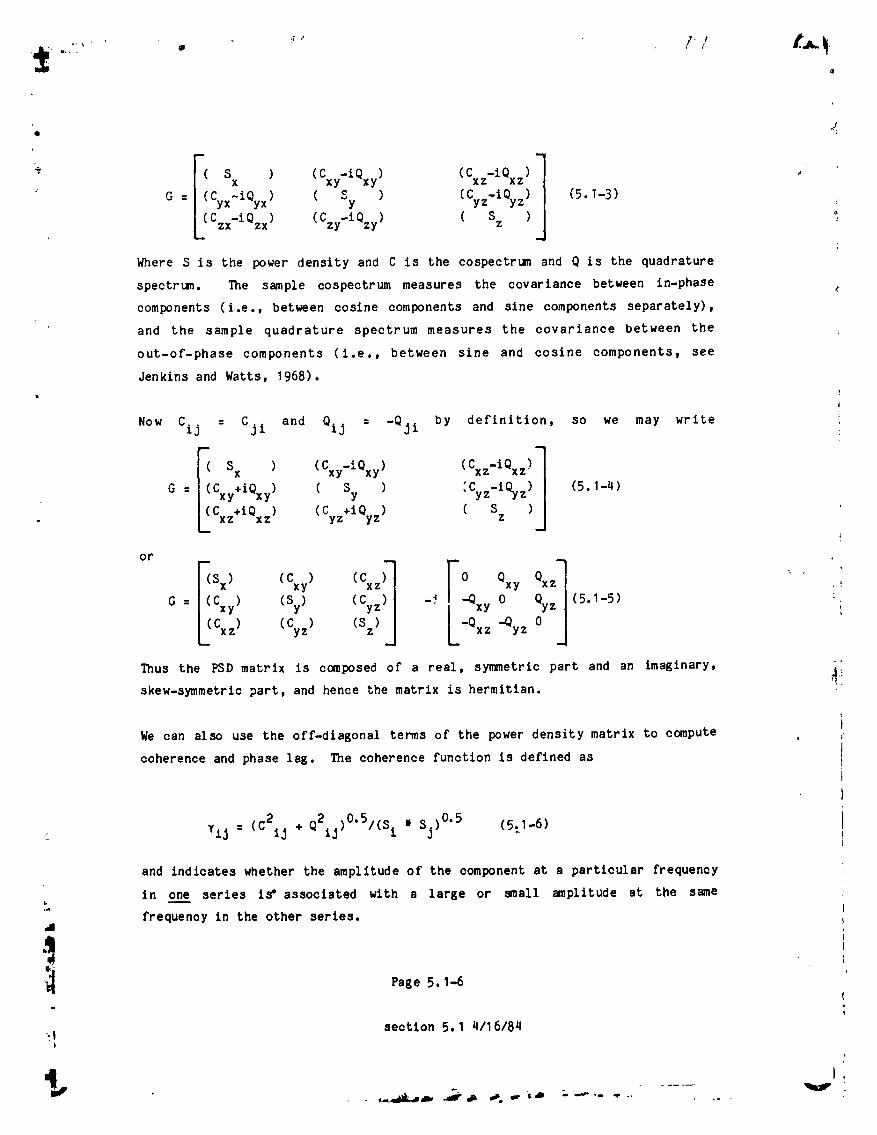
AIL _;
_. Sx ) (Cxy-iQxy) (Cxz-iQxz) ,
: G = /(Cyx-iQyx) ( Sy ) (Cyz-tQy z) (5.1-3)
(Czx-i Qzx) (Czy-iQzy) ( Sz )
Where S is the power density and C is the eospectrum and Q is the quadrature
spectrum. The sample eospectrum measures the covarlance between in-phase
components (i.e., between cosine components and sine components separately),
and the sample quadrature spectrum measures the covarlance between the
out-of-phase components (i.e., between sine and cosine components, see
Jenkins and Watts, 1968).
Now Cij = Cji and Qij = -Qji by definition, so we may write
F Sx ) (Cxy-iOxy) (Cx,-iOxz)]G = I(Cxy+iQxy) ( Sy ) :Cyz-tQy z) (5.1-4)
I (Cxz+iOxz) (Cyz+iQy z) ( Sz )
or
: LXY yzG I(Cxy) (Sy) (Cy z) -_ 0 (5.1-5) :.
J Cxz) (Cyz) (Sz) -Oxz "Oy z
Thus the PSD matrix is composed of a real, symmetric part and an imaginary, _i
skew-symmetric part, and hence the matrix is hermltian.
We can also use the off-diagonal terms of the power density matrix to compute
coherence and phase lag. The coherence function is defined as
YiJ : (c2 (5.1-6),_, iJ + Q2ij)0"5/(Si* SJ)0"5
and indicates whether the amplitude of the component at a particular frequency
in one series is* associated with a large or small amplitude at the sameL --
frequency in the other series•
Page 5.1-6i
_! section 5.1 4/16/84b
,......_,m,-,J'_ ,_. ,,,..;,i,---,-,..., ,- . _ "
1984026903-035

_' t"l
!
1
:/
Iand phase angle or phase lag in degrees is defined as
i :'_ @tj = (I801_)tan-I (qijlCij) (5.1-7)i
1 and indicates whether the frequency components in one series lead or lag the!
componentsat the same frequency in the other series.i
Operator SPECT computes the FSD matrix by using up to the first four (q)
complex series in the file generated by Operator FFT and in turn generates allr
possible permutations of the power and cross spectra using equation 5.]-8
belowi note that i is the index for the individual elements of each time
series, and j is the series index.
P(l,J,k) : XNORMIX(i,j)WmX(i,k) (5.1-8)
|Note: X(i,j) = Complex Conj.,
where ){NORM: 2/((2WNPTS-2)Iw2),thus folding the negative power and adding it
to the positive. For i=I, XNORM = I/((2iNPTS-2)m=2).
Example
For the case of three (3) time series, each containing 11 points (NPTS=11),i
these matrices are generated in the following fashion. Note that the time .__i
series, after being Fourier transformed (OperatorFFT), consists of 6 cc.mpiex
values of X(J). Note that for a given value of the time series index i, Eq.
5.I-8 produces from the Fourier transformedith elements of the three paralleli
series all possiblepermutationsof auto and cross power spectra.
|' P(1,1,1) : XNORM_X(1,1) iX(l,1)
IIP(1,1,2) = XNORMmX(1,1)reX(l,2)
P(1,1,3) = XNORMmX(1,1)%X(1,3)|
P(1,2,2) = XNORMIX(1,2) tX(1,2)I
P(1,2,3) = XNORM_X(1,2) reX(l,3)m
P(1,3,3) = XNORMiX(1,3) IX(l,3)
P(2, 1, 1) = XNORMIX(2,1)ltX(2, 1) \
"'" Page 5.1-v
'i
section 5.1 q/16184
1984026903-036

j_
i rl!
f
P(5,3,3) = XNOHM•X(5,3)uuX(5,3)
P(6,1,1) = XNORM*X(6,1) *X(6,1)
P(6,1,2) = XNORMmX(6,1) reX(6,2)m
P(6,1,3) = XNORMmX(6,1) •X(6,3) _"
P(6,2,2) - XNORM•X(6,2) reX(6,2)• /
P(6,2,3) = XNORM•X(6,2) •X(6,3)
P(6,3, 3) -- XNORM•X(6,3) •X(6,3)I
For the above caleulatlons Operator SPECT would generate the set of PSD
matrices shown below• Note that these Matrices are hermltian so we only
compute the upper right portion:
i:6 P(6,2,2) P(6,2,3)I
P(6,3,3)J
c5,1,2 PC ,1,3;]i=5 P(5,2,2) P(5,2, 3)I
P(5,3,3)| ' '
P(,,I,1) P(4, I,2) P(,,I,3)'I
i=4 P(4,2,2) P(4,2, 3) /
P(4,3,3)J
(3,1,1) P(3,1,2) P(3,1,3)Q .
1--3 P(3,2,2) P(3,2,3) I t..1
P(3,3,3)J I
P(2, 1,1 ) P(2, 1,2) P(2, 1,3) i I;11=2 P(2,2,2) P(2,2,3)
P(2, 3,3
P(1,1,1) P(1,1,2) P(1,1,3) 1
1=1 P(1,2, 2) P(1,2, 3)
P(I,3,3)
Page 5.1-8
&
section 5.1 4/16/84
1984026903-037
J_%
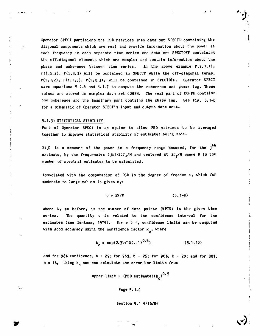
_.- Operator SPErT partitions the PSD matrices into data set SPECTD containing the "
diagonal components which are real and provJde information about the power at
C each frequency in each separate time series and data set SPECTOFF containing
i the off-diagonal elements which are complex and contain information about the
_' phase and coherence between time series. In the above example P(i,1,1),
P(i,2,2), P(i,3,3) will be contained in SPECTD while the off-dlagonal terms, :
P(i,1,2), P(i,1,3), P(i,2,3), will be contained in SPECTOFF. Operator SPECT
uses equations 5.I-6 and 5.I-7 to compute the coherence and phase lag. These ,
values are stored in complex data set COHPH. The real part of COHPH contains
the coherence and the imaginary part contains the phase lag. See Fig. 5.1-5
for a schematic of Operator SPECT's input and output data sets.
t
5.I.3) STATISTICAL STABILITY
Part of Operator SPECf is an option to allow PSD matrices to be averaged
; together to improve statistical stability of estimates be__n_made.
, X(j_ is a measure of the power in a frequency range bounded, for the jthIi
estimate, by the frequencies (J+I/2)f_M and centered at Jff/M where M is the
number of spectral estimates to be calculated.
Associated with the computation of PSD is the degree of freedom u, which for '
moderate to large values is given by:
u = 2N/M (5.1-9) ;
where N, as before, is the number of data points (NPIS) in the 8ivan time
series. The quantity u is related to the confidence interval for the t!
estimates (see Sentman, 1974). for u > 4, confidence limits can be computed
with good accuracy using the confidence factor kc, wherei
k = exp(2.3b/lO(u-1) 0"5) (5.1-10)c
and for 98_ confidence, b : 29; for 96%, b : 25; for 905, b : 20; and for 805,
b = 16, Using k one can calculate the error bar limits from
upper limit = (PSD estimate)(kc )0"5
r
" Page 5.1-9
1
section 5.1 4/16/84
1984026903-038

0.5lower limit : (PSD estlmate)/(k c)
For example, if N : 1500 samples and M : 60 spectral estimates, giving
v : 2NIH : 50
then kc = exp(O.O329b) and, for 90% confidence, (kc)0"5 = 1.390 and 11(ke)0"5
= 0.719. The PSD estimate would thus be multiplied by the factors 1.390 and
0.719 to obtain error bar upper and lower limits, respectively.
Note the relationship between data set SPECTD, when not averaged, and the real
part of data set FFTMP (see Section 6,FFT Operator); SPECTD :
2*(FFTMP/(2*J-I))*a2, where J = the number of points in the FFT including zero
frequency.
5.1.4) OPERATOR EIG, EIGENVECTOR SYSTEM
Users of spectral analysis techniques are often interested in applying them to
the study of wave phenomena. In such cases it is usually necessary to
investigate the fluctuation characteristics of the individual components of a '
vector, not only relative to a physically-defined set of coordinates but also :;
relative to one which is defined by the directional properties of the
fluctuations themselves. For the ease of an ideal elliptically-polarized
plane wave, for example, there is no fluctuation perpendicular to the wave _,:
front, and a maximum level of fl,,etuation along one direction parallel to the
wave front. There is thus a preferred coordinate system which most perfectly
reveals the nature of such a wave.
Such an analysis is implemented using an elgenvalue and eigenvector
calculation, In such a calculation, the characteristic variance ellipse (see
Fig. 5.1-6) is determined, to the extent possible; the principal axes of the
ellipse are the directions of maximum, Intermediate and minimum fluctuation,
respectively. To obtain eigenvalues and elKenvectors one needs only to
diaEonalize the real part of the PSD matrix, i.e., the real part of Eqn.
_5.1-5) For this purpose, IDSP employs the subroutine EIGRS, which is an IMSL
(International Hathematlcal and Statistical Libraries Inc., see Edition 8,
Page 5.1-10
section 5.1 4/16/84
I..
1984026903-039

Vol. 2, Chapter E) FORTRAN routine which computes and returns the eigenvaluesb
and associated eigenvectors of a real symmetric matrix. The eigenvalues are
the variances in the three principal axis dlreotions (see FIE. 5.1-6). EIGRS
does not order the eigenvalues and eigenvectors aceordin 8 to maximum,
intermediate and mimimum, however| this is accomplished in subroutine DIAG.
The eiEenvectors Vj are labeled with the indices JMAX, JMID, and JMIN,
respectively, in the orderin8 process. When used in conjuction with spectral
analysis, this process is carried out separately and independently for each
spectral estimate (each frequency bin). Thus the directions of interest can
be different at each frequency and FiE. 5.1-6 is for a particular frequency, f.
For the computation of parameters which characterize the polarization
properties of the fluctuations (see FiE. 5.1-7), we transform to a coordinate
system defined by the eigenvector system. This can be done in one of two
ways, either using the standard eigenvector definition In terms of the
principal axis system or using a special definition appropriate for data in
"mean field coordinates', which are defined in the description of operator
MNFLD (see Section 6). These systems are further described below.
1) Standard Ei6envector System- Under this option (the default mode), the
standard eigenvector definition developed above is used.
From this definition a matrix R can be derived for transformation of data from
the input coordinate system to the eigenvector system:
V(I,JMAX) V(2,JMAX) V(3,JMAX)
R : V(I,JMID) V(2,JMID) V(3, JMID) C5.1-11) ',
• ii
V(I,JMIN) V(2,JMIN) V(3,JMIN)
Where VCi,JMIN), i : 1,2,3, is the unit vector in the minimum varlance
direction.
This matrix is that.used to transform both the real and imaginary parts of the
"" Page 5. I-II !
section 5, 1 4116t8q
1984026903-040

J_
, PSD matrix data sets (SPECTD and SPECTOFF). Polarization par_neters are
computed according to the formulation described under option (2) oelow.
2) Mean Field Ei_envector S_stem- Use of this option is valid only if the data#
analyzed have been transformed to the Mean Field Coordi,ate System by use of
operator MNFLD (see Section 6) prior to application of EIG. This will have
set the switch MFIELD = I, which automatically activates the appropriate
elgenvector derivation procedure.
In this case, the ordering of eigenvalues and eizenvectors in DIAG will lead
to the definition
kI = V(I,JHIN)
k2 = V(2,JMIN) (5.1-12) _
k3 = V(3,JdIN).
A
The unit vector k gives the wave normal vector direction in the ease of a wave
analysis, and is here taken as the direction of minimum fluctuatlon, i.e., the
direction given by the elgenvector asslclated with the minimum elgenvalue, and
is one of the set of eigenvector coordinates.
For data in mean field coordinates, the matrix R can be derived wnlch
transforms the real and imaginary parts of the PSD matrix data sets (SPECTD
and SPECTOFF) to (mean field) eigenvector coordinates. In this case, R Is
expressed in terms of the components (kl,k2,k3) of R only'.
u q
4" k p _
2 2
i
k2 -kI 0 (5. :-13) i
+k 2 +k '.
k 1 k 2 k3
Page 5.1-12
section 5.1 4116/8q
1984026903-041
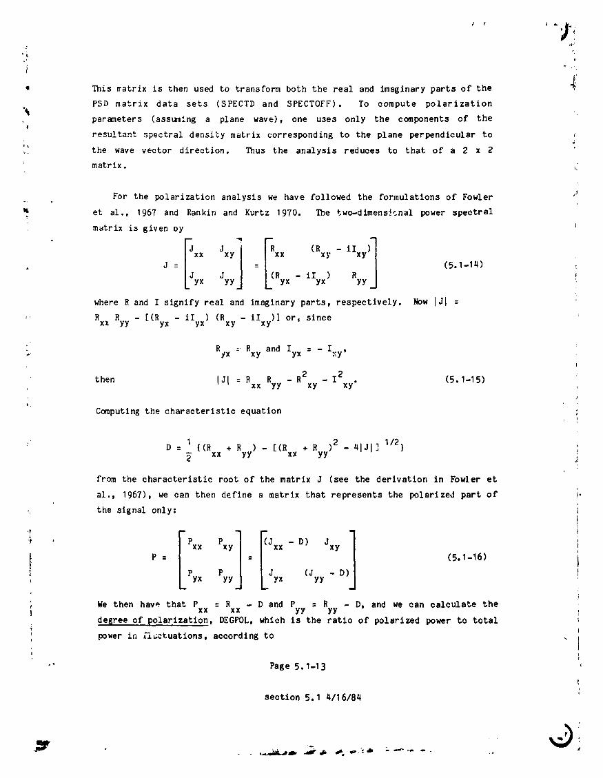
I
l
• This _atrix is then used to transform both the real and imaginary parts of the ;'_i
PSD matrix data sets (SPECTD and SPECTOFF). To compute polarization
parameters (assuming a plane wave), one uses only the components of the
resultant spectral density matrix corresponding to the plane perpendicular to
_ the wave vector direction. Thus the analysis reduces to that of a 2 x 2
matrix.
: For the polarization analysis we have followed the formulations of Fowler "'
et al., 1967 and Rankin and Kurtz 1970. The two-dimens_cnal power spectral
matrix is given Dy
xx xy xx (Rxy - t xy• J : : (5.1-1q)
L yx YY/ L(Ryx- iZyx) YYJ !i
where R and I signify real and imaginary parts, respectively. Now IJ[ =
:- R R - [(It - iI ) (R - lI )] or, sincexx yy yx yx xy xy
;, Ryx = Rxy and Iyx = - Ixy,
R - R2 - 12 (5.1-15)then IJ[ = Rxx yy xy xy"
t
Computing the characteristic equation i
D : 1 {(R + R ) - [(R + R )2 - "lJI ] 1/2}xx yy xx yy
from the characteristic root of the matrix J (see the derivation in Fowler et
al,, 1967), we can then define a matrix that represents the polarized part of i"
•. the signal only:
} ' Pxx Pxy xx - D) Jxy
P = : (5.1-16)
, Pyx Pyy L yx (Jyy - D)
, We then have that P = R - D and P : R - D, and we can oalculate theI xx xx yy yy
de6ree of polarization, DEGPOL, which is the ratio of polarized power to total
' power in Cz_ctuations, according to
i
Page 5.1-13
{i
section 5.1 q/16/84
1984026903-042
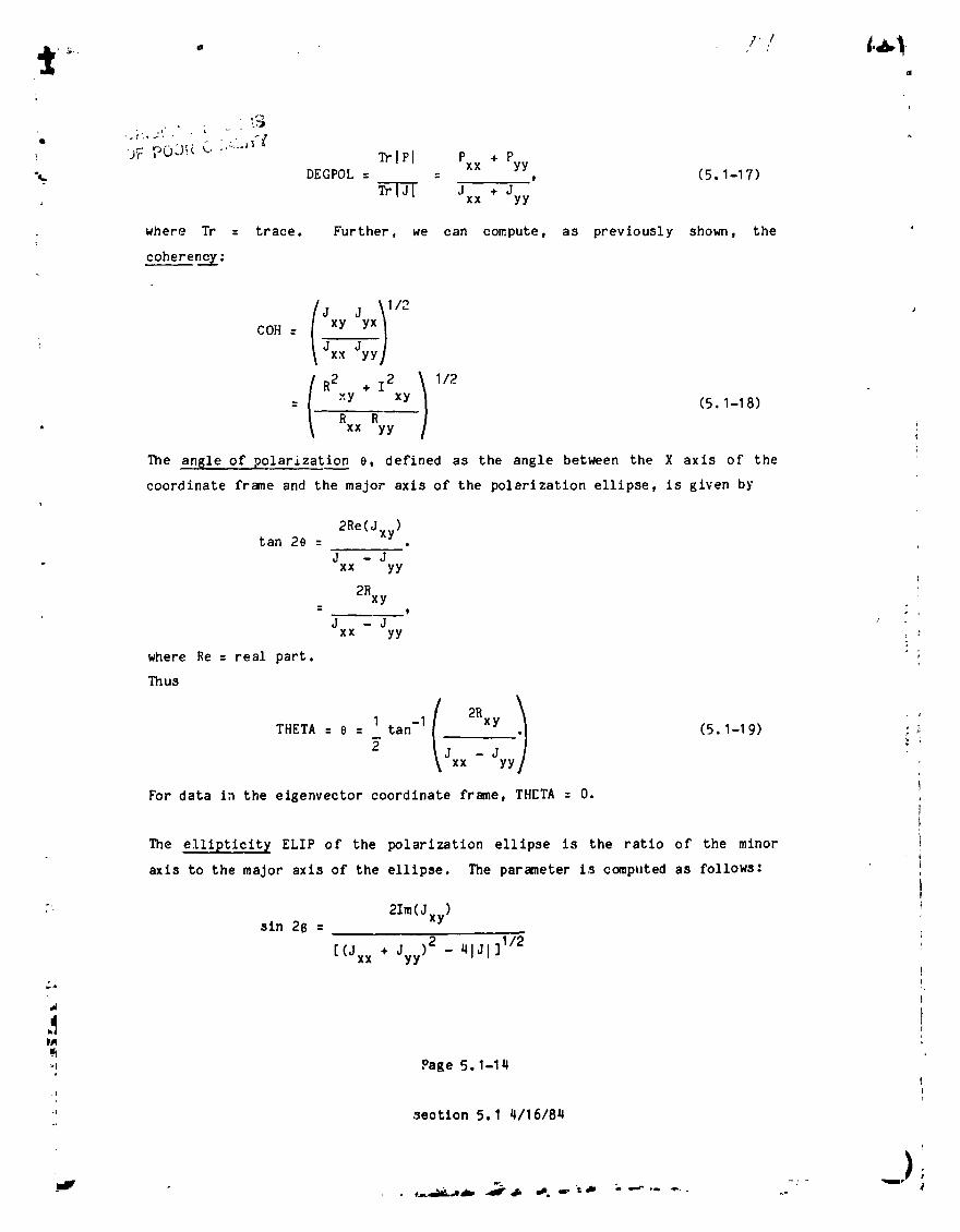
/1 o
,_
OF PO-._!( C '.-,'-"{_'_. 'rr {P{ P + Pxx yy
"_ DEGPOL = = , (5.1-17)
J +J: xx yy
where Tr : trace. Further, we can compute, as previously shown, the
coherency:
j Jyx\1/2• COH = xy l
Jxx J--_y]
R2 + 12 .) 1/2
xy xy= (5.1-18)
RXX R• yy !
The an_le of.polarization 0, defined as the angle between the X axis of the
coordinate frame and the major axls of the polarization ellipse, is given by
2Re(Jxy)tan 2e =
. J -Jxx yy
2Rxy= t
J -Jxx yy , :
where Re : real part. • ;
Thus
THETA : 0 : ....I tan-1 x (5.1-19)
2 Jxx yy/
For data in the etgenvector coordinate frame, THETA = O.
The elliptlclty ELIP of the polarization ellipse is the ratio of the minor
axis to the major axis of the ellipse. The parameter Is computed as follows:
:: 2Im(Jxy)sin 2B =
[(Jxx + jyy)2 _ 41Ji ]1/2
,a
_ Page 5.1-1q
"' _ectlon 5.1 4/16/8qH
),I
1984026903-043
OF PCO;:.Q;-r-,L__-:"
-21xy
f
[(Rxx + Ryy )2 - 41JI]1/2
where Im = imaginary part. Thus
B = _ sin -1 (5.1-20) ,
2 32 _ 41Ji]i/2and (Rxx + Ryy
ELIP : tan Isl. (5.1-21)
The sign of B gives the sense of the polarization relative to the vector field
being analyzed. This is shown, along with the corresponding phase angle
value, in the Table 5.1-I.
TABLE 5.1-I
Left-handed Right-handedPolarization Polarization
Phase lag Cxy 90° 270"
R • i_ positive S negative B positive
• _ negative S positive B negative
From th_s table we see that we can check results on the sense of polarization
relative to the vector field at a given frequency for consistency between the
computed phase angle at that frequency and the sign of B (dependent on the
sign of _ • _). Since B is not one of the output parmieters available in data
set EIGPARM (see last paragraph of this Section), the sign of B has been
assigned to DEGPOL, which is otherwise a positlve definite quantity. Only the
absolute value of B can be obtained from the quantity EL!P. The value of _._
= BDOTK is an additions] output quantity whzch depends for its sign on the
sign of _. The sense of _ (whether it is positive or negative) is completely
arbitrary as determined by subroutine EIGRS. Thus it is necessary to adopt a
convention for the sign of _. This is done by leans of the optional parameter
KCON. It allows the u_er of operator EIG to either force _ always to be
outward rather than inward-directed relative to the sun or to force _ always
to have a component in the +_ rather than the -§ direction (unless R A _)" A
_,,'- Page 5.1-15
section 5.1 _1/16184
,..,,,_m. _ ,#* =_. ,"- =ab ..-
1984026903-044
:I
more detailed description of KCON is given in Section 6.9.
I
A second unit wave vector _ is independently computed using the method
described by Means, 1972. This technique derives the components of _ using
I only the imaginary part of the spectral density matrix. Good agreementI
between the results from the two methods has been taken as an indicator that ,
the wave normal vector was well determined. The analysis output also includes/
the slgnal-to-nolse ratio defined by Means, 1972 as
I J +JSNR = xx yy (5.1-22)
JZZ
where J + J is the trace of the 2-dimensional matrix defined by equation} xx yyr (5.1-14) and J is the additional diagonal element of a 3 x __ matrix that
Z_i
: includes the _ direction.
In studies of magnetic turbulence, a useful quantity (because it is an!
tnvariant of ideal MHD turbulence) is the magnetic helicity. The magnetic
hellcity is a measure of the topographical linkage of the magnetic field and
is closely related to the polarization (see Moffatt, 1978). Techniques of
determining the magnetic helicity can be found in Matthaeus and Goldstein,
1982 and Mat_haeus et al., 1982. If we denote by H (f) the reduced magneticm
heliclty sppctrum, then a parameterzation of Hm bounded by -+Ican be defined as.,,,?
SIGMA = fHm(f)/trlGl (5.1-23) ::
where f is frequency and G and Qxy are from Eq. 5.1-3 and Hm(f) = 2Qyx(f)/f, 1where it is assumed that the spectrum has been reduced to the z axis (see y
M_,tthaeus and Goldsteln, 1982 and Hatthaeus et al., 1982 for more details).
Note: Do not use the mean field option if _ou want to compute SIGMA- results
will be meanin61ess.
Data set EIGPARM contains scaler quantities DEGPOL, COH, ELIP, THET&, TRTOT,
SNR, BDOTK, and SIGMA. EIG also creates data set EIGVEC which contains in
series I-3, the first three components of the eigenvector corresponding to the
direction of minimum variance for that mode. Series 4-6 are the eigenvalues \
Page 5.1-16 !i
section 5.1 4/16/84
,)L
#
_ ,=.4,_.,#db, 4 _ _ ,'P- = ,t, :,. --_- ,- ",,,;.. - " ,_,
1984026903-045
(minimum, intermediate and maximum, respectively), Also created by operator
EIG is data set EIGVECI which contains the three components of the elgenveetor
corresponding to the intermediate direction (series I-3) and the three
eigenvector components corresponding to the m6xlm6_ direction or" variation
(series 4-6). For a schematic of operator EIG and it data sets see Fig. 5.1-8.
5.1.5) EXAMPLE: THE USE OF IDSP IN THE ANALYSIS OF WAVES IN DEEP SPACE DATA
In this section we provide an example of the application of the IDSP to a
specific scientific research task. In this case use of IDSP assisted in
analyzing magnetic field measurements made by the Voyager 2 spacecraft 11 days
after its closest approach to Saturn on August 27, 1981. At that time, low
frequency waves were detected in the _agnetic field, apparently in association
with enhanced flows of charged particles from the direction of Saturn. Fig.
5.1-9 shows the magnitude B of the total magnetic field as well as that of
each of the three orthogonal vector components of the field in a hellographlc
coordinate system during a 2q-hour period. The data plotted are q8-second
averages of initially 60 millisecond measurements. Large amplitude waves with
a period of approximately 1.6 hours on average can be seen both in the
magnitude and each of the components of the field. As noted on Fig. 5.1-9,
higher frequency fluctuations of the field were detected also during a six
hour period beginning at midday. They will be investigated later in this
example. The analysis of both types of waves was accomplished via the IDSP
and will be illustrated.
The data shown in Fig. 5.1-9 were processed using operators SETUP, INTERP and
GRAPH. Using operator WINDOW, the effect of different types of windows on the
data was examined. In the examples shown, the rectangular (default) window Ip
option was used. The data were spectrum-analyzed using the FFT and SPECT
operators, with 3 points forming each spectral estimate in the latter
operation (6 degrees of freedom). Fig. 5.1-10 shows part of the output of
SPECT in the form of the power spectral density matrix diagonal terms plotted
using GRAPH. They constitute the spectra of the field veotor components and
the field magnitude (data set SPECTD). Shown along with th_ PSD of B for
comparison is the trace of the PSD matrix (calculated using operator TRACE),
which is a composite of the individual component spectra. The peaks of each \
Page 5.1-17
section 5,1 5/23/84
1984026903-046
+j
of the spectra, corresponding to the quasl-slnusoldal waves in the time
%. domain, occur In a band centered at a frequency of 1.75 X 10⁻⁴ Hz.
The properties of the waves were studied further by means of the EIG operator.
A subset of the results are shown in Fig. 5.1-11. Selected parameters were
plotted from d_ta set EIGPARN using operator GRAPH. Their values are shown
for a restricted region of the frequency domain near the peak frequency, where
in this case, a linear frequency scale has been chosen for display purposes.
For reference, the corresponding segment of the PSD trace is plotted in the
top panel. The most relevant quantities resulting from the elgenfunctlon
analysis are shown below the trace: (I) Degree of polarization (DEGPOL), (2)
. cosine of the angle between the wave normal vector _ and the magnetic field
vector _ (Cos_ = R • _ = BDOTK where _ is known only modulo 180"-see
discussion following Table 5.1-Ij, and (3) the elllptlclty of the polarization
ellipse (ELIP). The definitions of these quantities were given in Eqns.
5.1-17, 5.1-21 and the text following those equations.
A vertical band one spectral estimate wlde delineates the relevant region on
each parameter curve in Fig. 5.1-11. Note that DEGPOL has been plotted with
both positive and negative values. This is because this otherwise
positive-definite quantity is multiplied by the sign of B (Eqn. 5.1-20). The
wave is seen to be highly polarized (DEGPOLpeak = 0.95). An average value ofI
BDOTK over the peak gives a = 112°; thus the wave is propagating at a large i
to the magnetic field direction. Positive values of DEGPOL at the waveangle
frequency, together with negative values of BDOTK, suggests left hand (LH)
polarization in the spacecraft frame of reference (see Table 5.1-1 and
following text)• However, as indicated following Table 5.1-1, in running gIG a
convention forces _ to have a particular sense of direction. The user must be
careful that this direction is physically reasonable in terms of its
implications for the specific phenomenon being studied. In this ca_e, as
would be usual for studies of waves in the solar wind, the analyst set KCON =i
I (away from the sun) This also forced _ to have a component toward Saturn,i •
the source of the beam of ions excltln8 the waves. But, since the waves
should have the same sense of direction as that or ion flow in the beam,
should in fact be directed away from Saturn. Thus we are led to the
intepr-etatlon that in this case the wave was actually right hand (RH)
Page 5.1-18
section 5,1 5/23/8_
1984026903-047

.Ab.,....,., , /"I L.%
polarized (corresponding to a = 180 ° - 112 ° = 68°). Finally, an average valueof ELIP = 0.7 is found at the peak, indicating that the wave is much closer to'iI being circularly polarized (ELIP : 1.0) than linearly polarized (ELIP : 0)..!
It is sometimes useful to replot the original data in a coordinate system
defined by the set of ,,igenvectors corresponding to the directions of maximum,
intermediate and minim_, oscillation in the wave. This is accomplished using
the ROTATE operator on t_e original (in this case INTERP) data set, with the
i new coordinate system provided by the EIGVEC and EIGVEC1 data sets. The
specification given in this case was: ROTATE INTERP 1,2,30 NFREQ=16. The
resulting data are shown in Fig. 5.1-12, with XE being in the direction of
i maximum variation and ZE in minimum variation direction.
As mentioned earlier, in Fig. 5.1-9 and 5.1-12, an interval of higher
frequency fluctuations is seen superimposed on the 1.6 hour period waves. The
_i maonetic field data for the 6.4 hour interval in which this second wave modeocurred are plotted on an expanded time scale in Fig. 5.1-13. In this caseJ
higher tlme-resolution data (9.6 sec averages) are shown. Approximately 4
cycles of the low frequency oscillation are still seen modulating the higher
; frequency fluctuations, which can be seen to be of much higher amplitude in
I the vector components than in the field magnitude. To facilitate the study of
I higher frequency variations, we removed the low frequency excursions by high
_i pass filtering the data set shown in Fig. 5.1-13. The procedure for designing
and applying digital filters is discussed and illustrated in Section 5.2. The
filter specifications that were entered into data set FORO58. DAT and used by
operator FILDES for this task are as follows:
125, 1,2,0
0.0,0.002,0.02,0.5i
0.0, 1.0182.0, 1.0
: This iS a filter with 125 coefficients, of the multiple passband/stopbandn
type, with one stopband and one passband (for which the start ano stop3, normalized frequencies ar_ (0.0, 0.002) and (0.02, 0.5), respectively). The
grid density is set at 16 (input specification of 0 gives default value ofJ
Page 5.1-19
section 5.1 5/23/8q
.... _m_ 4r4_ _. _.'=a* _-'=,- _..,
1984026903-048
f
16). Ideally there is complete attenuation in the stopband and no attenuation
in the passband (0.0, 1.0), and, finally, a relative weighting of 182 in the ,
stopband to 1 in the passband is used.
i
Fig. 5.1-1q illustrates the frequency response of the filter generated for '
this task. Because the higher frequency oscillatlon to be studied was still
at a relatively low value of normalized frequency (_ 0.03), the passband
response was designed to rise steeply to a value of I near zero normalized
frequency. This requirement tightly constrained the values that could beI
given to most of the filter design parameters. The bandedge array values
(EDGE(i), I=1,4) and band weight functions (WTX(1), WYX(2)) could be adjusted,
however, within the given constraints, to permit to some degree the
maximization of attenuation in the stopband and minimization of ripple
amplitude in the passband. Because of the fact that the two factors work
against one another for a given filter configuration as the weights are
varied, reduction of passband ripple beyond a given point Is limited by the
onset of incomplete stopbsnd attenuation. Conversely, stopband attenuation is
limited by increasing distortion of the spectrum by the increase in passbandI
ripple amplitude. Any such distortion is undesirable and may not be totally
eradicable if the number of filter coefficients cannot be increased further
and/or the bandwidths cannot be further adjusted, including the width of the
transition band (see Fig. 5.2-1). _ ;
A study was performed (using operator FILOPT, see Section 6) to provide
insight Into the degree of tradeoff possible in this example between stopband ' :
(band 1) attenuation and passband (band 2) ripple. While all other designt
parameters were held fixed, WTX(1) and WTX(2) were varied over values ranging t.
from (1,100) to (1000,1), which, since the weights actually represent s ratio,
is equivalent to setting WTX(2) = 1 and varying WTX(1) over the range 0.01 to
1000. As described in Section 5.2, for a given set of parameter values,
FILDES generates a filter and lists its characteristics (as illustrated in
Table. 5.2-I). Among the output characteristics tabulated are the amplitude
deviations in each band, i.e., the delta 1 and delta 2 values. Although the
resulting values of each have been Influenced by the full suite of input
parameter values, and hence desired values may not be realized, the ratio is
predetermined by the bandwetghts, i.e., by definition deltal/delta 2 = _
Page 5.1-20
t
section 5.1 5/23/84
1984026903-049

i WTX(1)/WTX(2) (see Rablner _nd Gold, 1975, PP 197,199).
! 4'
From the amplitude deviations, the passband and stopband ripple amplitudes in
dB are computed (see Section 5.2 for definitions).I 4
i
In our tradeoff study we plotted the various passband and stopband ripple
combinations output by FILDES _s functions of the relative weight
WTX(1)/WTX(2). We used the dB values since they are directly comparable to the
desired performance specifications that enter as inputs into the filter
planning process (see Section 5.2). The resulting curves are shown in Fig. i
5.1-15. As can be seen, passband (PB) ripple is relatively flat over much of
the region of steepest increase (negative) in stopband (SB) ripple. For I
larger relative weights (>160), however, PB ripple rises steeply, and the i
continued SB ripple growth becomes less steep.
For our hlgh pass fllter, the stopband minimum frequency response (and hence
the level of attenuation) is that computed at zero frequency (see Plg.
5.1-14). This value is also a function of relative bandwelght, and, although
influenced by the stopband ripple amplitude, its variation wlth changes in
relative weight Is different from that of the ripple amplitude. The minimum
response (maximum attenuation) dependence on weight for this case Is
illustrated in Fig. 5.1-16. The curves shown in Fig. 5.1-15 and 16 can be
obtained by using INTERP on the output from the FILOPT operator and graphing
the results.
Although there are two distinct minima in the curve, the second, occurring at
a -elatlve weight of 182, was found to provide the most complete attenuation
Iof the low frequencies in the data. From Flg. 5.1-15 It Is seen that for a
weight of 182 the passband ripple has not yet grown large (0.13), but the
stopband ripple is relatively large (-82), as desired. This was thus
considered to be the optimum state for the given bandedge configuration. It
is worth noting that prior to selection of bandedges (0.0,0,002,0.02,0.5), we
investigated the conflguratlon (0.0,0.001,0.01,0.5). For that case the ripple
vs. relative weight diagram was similar in general form to that of Fig.
5.1-15, but differed considerably in detail. The stee increase In PB ripple
began at a low value of relative weight (q.5). The optimum values of SB and \
--" Page 5.1-21
section 5.1 5/23/84
1984026903-050
PB ripple were -40 and 0.35, respectively, considerably less effective than
those possible with the final bandedge configuration chosen. Thus it is also
important to optimize bandedge values as well as band-weightlng factors. It
should be noted that a set of desired stopband and passband ripple amplitudes
will end up being the achieved characteristics of a particular filter
configuration only if the total set of design parameters can accomodate the
realization of those values.
Upon completion of the tradeoff and optimization procedure for our high pass
filter design, operator FILTER was called to apply the resultant filter to the
Voyager data. The filtered data set is plotted in Fig. 5.1-17. It is clear
that the filter has successfully removed the modulation. The remaining
fluctuation is quite variable in amplitude, and the frequency is evidently
variable as well. This may be the result of a superposition of several
fluctuations of different _plitudes and frequencies. The corresponding
spectral characteristics _ _hown in Fig. 5.1-18, where 5 points were used to
form each estimate (IC degrees of freedom). The rising trend of the PSD at
low frequencies < 10-3 Hz in each case is the result of the fllterlng of the-3
data. The weakly dominant frequencies in the fluctations (3.q to 3.9 X 10
Hz; period = _.3 to 4.9 mln) are denoted by the vertical dashed line: as can
be se_n, this peak _s only a single feature of a broad, highly structured
shoulder on the o_era]l sp_rum, as was anticipated from the appearance of
the data
Selected results of the eigenfunction analysis are plotted in Fig. 5.1-19
together with a ,rtion of the trace of the PSD matrix. As in the case of the
1.6 hour period waves, the _ 5 mln fluctuations are hlghly polarized (Maxlmum iF
DEGPOL = 0,8) and elliptical (Maximum ELIP : 0.75), polarization in thei
spacecraft reference frame is rlghthanded (RH), as indicated by +DP and
+BDOTK, and the waves are propagating at a fairly large angle to _ (average
BDOTK = cos a _ 0.57 so a = 55°). Note that in this case KCON = 0 was
specified in running EIG, forcing E to have a component in the +_ direction.
Page 5.1-22
section 5.1 5123184
1984026903-051
¢
5.1.6) OPERATOR MEM (MAXIMUM ENTROPY METHOD) .J
The maximum entropy method (Operator M_) for spectral estimates was
introduced by Burg in 1967. Its purpose was to increase the spectral
resolution when the length of the observed data record was short. :
Conventional spectrum analysis techniques usually window the autocorrelation,
append zeros and then Fourier Transform to obtain the spectral estimate.
Instead the MEM extrapolates the autoj3orrelation beyond the limited range of ;
the data to derive the spectral estimates at the desired resolution with
little or no interference from other frequencies.
The MEM power spectrum, P(f), can be described by the following expression
I
P AtP(f) = m
_ -.2,fnat) 2- 2...,a_.e z
n=1m"
P : output power of the prediction error filterm
a 's : m+1 prediction error filter coefficientsmn
At : data sampling rate
f = frequency
For details on how the filter coefficients are calculated see Anderson, 1974.
The equation is solved by stepwise iterative increase of the matrix _,
dimension from m-1 to m. The only remaining area of concern is choosing the
number of filter coefficients, m. If m is too small the power spectrum tends I
to be very _mooth, thus eliminating any additional resolution; if m is too I i
large, spurious information may be introduced into the spectrum The value ' I• i
2N/_n(2N) can be used as a default parameter. This was proposed by Berryman, }
1978 based on empirical evidence. Otherwise a trial and error approach is _ itedious alternative. I
T
b
"l-" Page 5.1,-23 ;
section 5.1 U/16t84
1984026903-052
REFERENCES:
1) Anderson, N., Shortnotes: On the calculation of filter coefficients for
maximum entropy spectral analysls, Geophysics, Vol. 3_99,No. I (February,1974), pp. 69-72.
2) Bergland, G. D., A Guided Tour of the Fast Fourier Transform, IEEESpectrum, July 1969.
3) Berryman, J. G., _.nolce of operator length for maximum entropy spectral
analysis, Geophysics, Vol. 43, No. 7 (December 1978), pp. 138q-1391.4) Brigham, E. 0., The Fast Fourier Transform, Prentice-Hall, Inc, Englewood
Cliffs, New Jersey, 1974.
5) Burg, J. P., Maximum entropy spectral analysis, presented at the 37thAnnual Interr,atlonalSEG Meeting, Oklahoma City, OK, October 31, 1967.
6) Fowler, R. A., B. J. Kotlck and R. D. Elliot, Polarization Analysis ofNatural and Artificially Induced Geomagnetic Mlcropulsations, J.Geophys. Res., 72, 2871, 1967.
7) Jenkins, G. M. and D. G. Watts, Spectral Analysis and its Applications,Holden-Day, San Francisco, 1968.
8) Lanczos, C., Applied Analysis, Prentlce=Hall, Englewood Cliffs, NJ, 1956.9) Lanczos, C. Discourse on Fourier Series, Hafner Publishing Co, New York,
1966.10) Matthaeus, W. H., M. L. Goldstein, Measurements of the rugged Invarlants
of magnetohydrodynamic turbulence in the solar wind, J. Geophys. Res.
87, 6011, 1982.11) Matthaeus, "d. H., M. L. Goldsteln, and C. Smith, Evaluation of magnetic
helicity in homogeneous turbulence, Phys. Rev. Lett_ 48, 1256, 1982.12) Means, J. D., Use of Three-Dimensional Covarlance Matrix in Analyzing the
Polarizatlon Properties of Plane Waves, J. Geophys. Res., 77, 5551, 1972.... '
13) Moffatt, H. K., Magnetic Field Generation in Electrically Conductln_Fluids, Cambridge Onlversity Press, N_, 1978. _.
lq) Otnes, R. K. and L. Enochson, Dl_ital Time Series Analysis, J. Wiley andSons, New York, 1972.
15) Rabiner, L. R., B. Gold, Theory and Application of Digital SignalProcessln_, Prentice-Hall Inc,, Englewood C_Iffs, "NJ, 1975. -
16) Rankln, D. and R. Kurtz, Statistical Study of Mlcropulsatlon Polarization,
J..Geoph_s. Res., 75, 5444, 1970.17) S_.ntman, D. D., Basic Elements of Power Spectre1 Analzsls, U of iowa
Preprlnt74-5,The University of Iowa, Iowa City, Iowa 522_ Jan. 1974. Ii
Page 5. I,.24
section 5.1 4/1 6184
_.mt_ _._ -t---i_ "'_ .....
1984026903-053

I
kAT) _:,r..... I
t:o AT 2_T • • • • • • • NAT:T
k=o 1 2 • • • • • • • • N
\ X( jfo )\
f=o fo 2fo " " • ff - • • • Nfo=fs
j=o ! 2 • • • N/2 • • • • NI
fo=I/T; fs=Nf ; T=NAT
FIG. 5.1-I
This drawing is after Bergland, 1969 and shows what happens when a time seriesx(t) is Fourier transformed. X(J) is, in general, a complex series. The time
series x(kAT) is assumed to be periodic in the time domain of period T. Tha
Fourier coefficients X(Jf 0) are periodic over fs" Each J should beinterpreted as a harmonic ndmber and each k a sample period number. Actual
frequency = Jfo" Actual time = kAT. When x(k) series is composed of real \.numbers, as it-often is, the real part of X(J) is symmetric (even function)
_,.. about the Nyqulst frequency f_z /2 and the imaginary part is antlsymmetrlc(odd function) about the Nyquls% Frequency.
PaRe 5.1-25
V .... , wj ;
1984026903-054

(z: ,_I.L,I_
%T_--- 20oo _,_ 5b.oo eb.oo _o.oo ,_o.ooIbo.ooDINS
_IG. 5.1-2
Shows the real part of the results of Fourler tremsformtn8 x(t) = 10 Cos(21mtSmkmaT) + 5 Sln (2wm2OmkmAT) eampled at 120 tJJes per seo. Note that th_
real part ts s_mmetrle about the Nyquist frequenoy, ff (i.e., BIN 120/2 = 60).
o
6
=o
o
'l
o
2,
'0_o- _b.oo _.oo 6b._o---_.0_ _bo.Oo ,_o.oo ,_._om BINS,
' FIG. 5.1-3
Sho_a the lu81r_mr_ pert of tbe reaulte o_' ieourler tr--afomlnll x(t) • %0 Cos(2_mtSakm&T) �5SJ.n (2_m2OSkm6T) Ulple4 at l;_O tJJU per ee_. Note t_t the
Imaginary pert Is mntlamtrlo about the II_q_let tr_i_.o¥, fr"
• _age 5.1-26I
)
1984026903-055
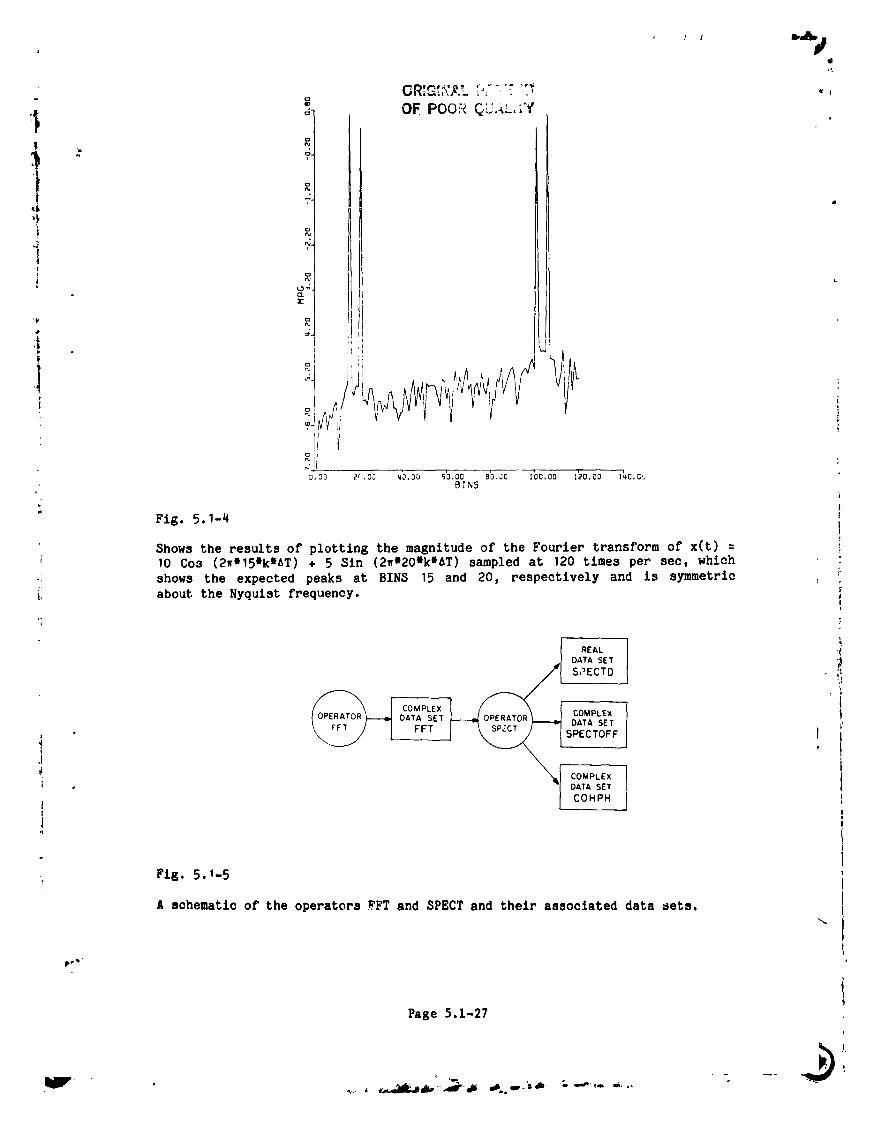
! I m,_.J
=l
OR;_r,\,k,_",- -.-" "v.0
:_ a OE PO0;_Q_._.L,;Y! 8
I 2" 6.
i ,
_L
_F
, /i
[
j! i
_,oo e;.o: _o.oo 5'o.oo e'o,Jo l'_o.oo 1}o.oo _'_o.:bBIN5
Fig. 5.1-4
Shows the results of plotting the magnitude of the Fourier transform of x(t) :i 10 Cos (2_*15*k*AT) + 5 Sin (2_m20*k*AT) sampled at 120 times per see, which
=L shows the expected peaks at BINS 15 and 20, respectively and is symmetrici about the Nyquist frequency.
SEALDATA SET
SPECTD i,i
COMPLEX COMPLEXDATA SETDATA SET ;,
i FFT SPECTOFF l,I j_i COMPLEX ti DATA SET
! COHPH I
,, Fig. 5.I-5 Ii
A schematic of the operators FFT and SPECT and their associated data sets. I
It
Page 5.1-27
1984026903-056

.: X.- Fig. 5.1-6
/ In the study of wave phenomena it is eoMon to investigate, using an-:-' elgenfunetton analysts, the _uotuatlons eharaet.ertsttos of the individual
co=portents of the veotor reletlve to the directional properties of the
fluotuatlon themselves. In suoh calculation the etgenvaluea detemtne theprincipal axes (o:',o==,o, =) or" the oharaeterlstte variance (polarization)ellipse at eanh frequency estimate. The etgenveotort define the coordinate
'_ system corresponding to the directions of maximum (X), intermediate (Y) andmtntmum (Z) osolllatlon in the wave at eanh frequency estimate. !
1984026903-057

,=
Y
t
I
Z
r"
LEFT- HAND POLARIZATION
Fig. 5, 1-7
Illustration of a plane, left-hand polarized wave, with front parallel to the
X-Y plane, shown at a succession of Limes t : 0 to t = q as.it propqates inthe + Z direction (toward left). The perturbation vector b rotates CCM as
/, viewed from upstream, its tip describing the polarization ellipse In each 360"-,.i rotation. Although _.he total field _ is not shown, this case corresponds to; _ " _ positive and _ negative. For right-handed waves propagatir_ in the + Z
direction, the rotation sense would be 04. In the case shown, the spatial
ortentatt,_n of the ellipse remains constant during the time interval of the, . ' propasation; in 8eneral, it may vary with time.
Pase 5,1-29
1984026903-058
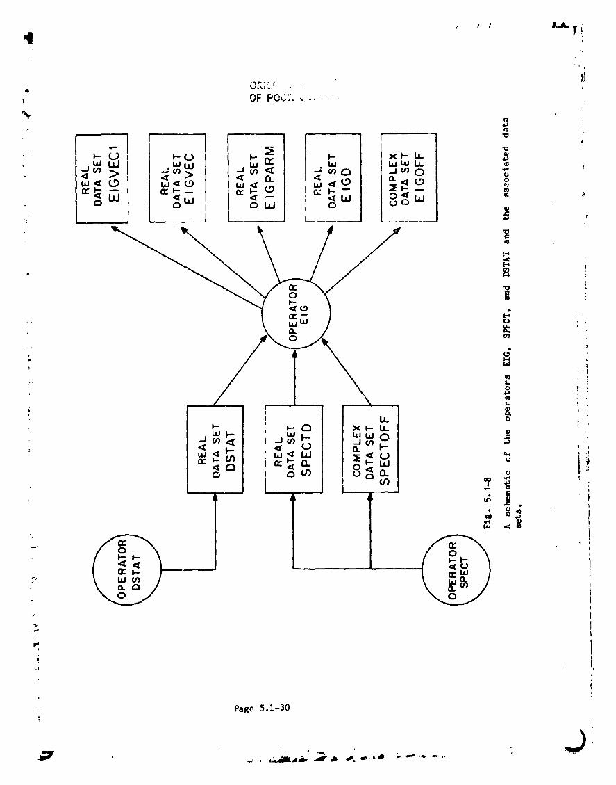
• , ._ a.._I..i
1984026903-059
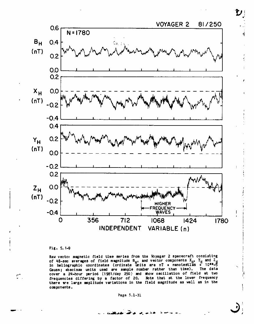
, ,tj.0.6 VOYAGER 2 81 / 250 .,.
N=1780 _(,
BH 0.4 - c-, .,.
(nT) 0.2 _'
0.0 i i j , , , i , , . ;0.2
X H 0.0
(nT) -0.2I
-0.4 , i , , i i , J i ,0.4
YH 0.2
. (nT) 0.0 t-0.2 i , i L I i i i i0.2
ZH 0.0
(nT) '"O.2 t HIGHER
M---FREQUENCY'_-0.4 I I I I I _AVES I I I IP
0 356 712 1068 1424 1780• INDEPENDENT VARIABLE (n)4
I
i Fig. 5. 1-9
Raw vector magnetic field time series from the Voyager 2 spacecraft consistingof qB-see averages of field magnitude BH, and vector components XH, YH and Z.in heltographl¢ coordinates (ordinate units are nT = nanotestl_s : lOeW-_ \Gauss; abscissa units used are ample number rather than time). The data
t'" cover a 2q-hour period (1981/day 250) and show oscillation of field at two i_:- frequencies differing by a factor of 20. Note that at the lower frequency
there _re large amplitude variations In the field magnitude as well as in thecomponents. !
Page 5.1-31
o
1984026903-060
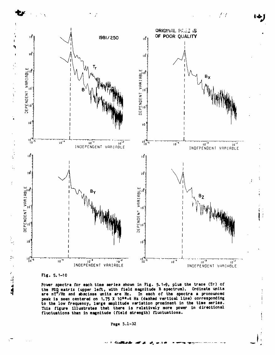
: ;' ,l"f L.IMjJW"
, I ORIGID_AL P;;.C-,"_ k_
" 1°21 1981/250 1o2! OF POOR QUALITY
,. I Tr
a_ Ia: Bx
a: I>ld: I >lO- [
I£3 I "'Z £3
_,o-! I z
" I,6 I ,o! I
I II I
'O'S '0"_ '0"_ '0"2 ,0 S ,0-_ 10-3 lO._
' INDEPENDENT VlqRIQBLE INDEPENDENT VARIABLE
I
id X,/f l_r I ;
,,_ . By m
_' _,Bz>10" '
£3 O _Z , Z
_,o" _,o IuJ "' I£b r'3
• I
• _o" _o" l
I
I
: I0 "_I ]0 "$ ..... JO ]O "_ ........... lO "$ |0 -2
INOEPENOENT VARIABLE INDEPENDENT VARIFtBLE
/
.i Fig. 5.1-10
Power spectra for each time aeries shown in Fig. 5. 1-9, plus the trace (Tr) o£
the matrix lef_, with field malinttude B spectrum). Ordinate units(upper ,
are nT'IHz and abscissa units are Hz. In each o£ the spectra a pronounced
peak is seen centered on 1.75 X lOae-q Hz (dashed vertical line) corresponding Jto the low frequency, 1erie amplitude variation prominent in the time series, iTI_iI £tgure illustrates that there ls relatively more power in dtreottonal
fluctuations than In m_l_nitude (field strength) fluctuations, i!
Page 5.1-32
i•;., _ _,,L,,_¢_I_ ,_r._ _. ,p. s_ " "--"=. "_-t..r................ v ..,,-- •
1984026903-061

I-.-0 0C3
-I.01.0 i
1984026903-062
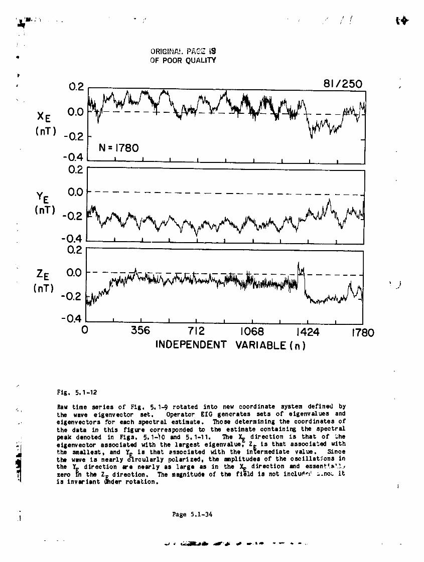
• OF POOR QUALITY
I'
• 0.2 81/250 .
XE 0.0
(nT) -0.2[_N =1780-0.4 , , , , , , , ,0.2
YE 0.0
(nT)-0.2__/W_',-0.4 , , i , , , lO.2
ZE 0.0 ..........:9
(nT) -0.2
-0.40 356 712 1068 1424 1780
INDEPENDENT VARIABLE (n)
J
Fig, 5.1-12
Raw time series o£ Fig. 5. 1-0 rotated into new coordinate system de£1ned byc_ the wave eigenvector set. Operator gIG generates sets of etKenvalues and_, ei£envectors for each spectral estimate. Those determining the coordinates of
the data in this Figure corresponded to the estimate contalnl_ the spectralpeak denoted in Fti&s, 5.1-_.0 and 5,1-11. The XE direction is that of _he
_ eilenvector associated with the largest etgenvalue, Z_ is that associa_.ed with
i the smallest, and Y_ is that _ssociated with the Intermediate value. S/nce
the wave is nearly circularly polarized, the amplitudes of the oscillations in
the Yr_ direction are nearly as lsrBe as In the XE direction and assent%'2,..,zero rn the Z_dtrectton. The magnitude of the field t8 not lnclu_*,# _,no_ itIs lnvartsnt Ohder rotation.
-" Pase 5.1-34.I
1984026903-063
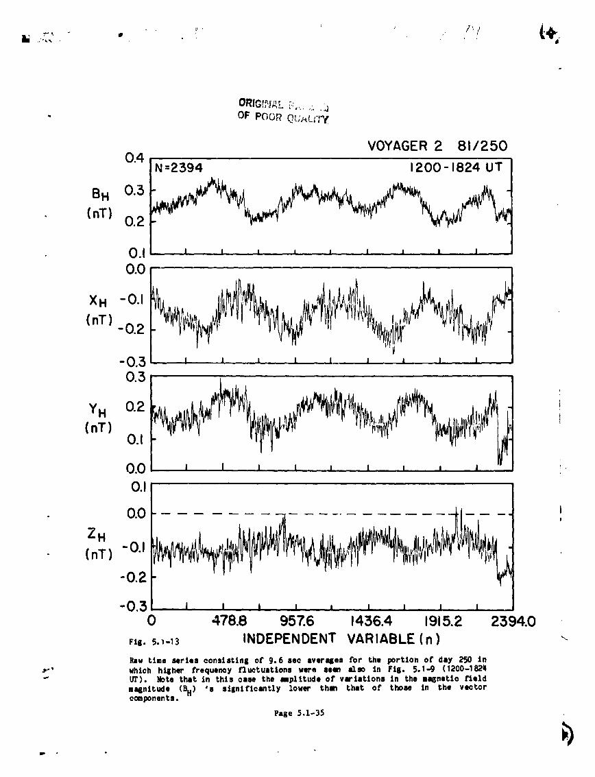
ORIG{NRL[.:,....-.+OF POOR Q,,;-_L,Fy
VOYAGER 2 81/2500.4
N=2394 1200-1824 UT
BH 0.3
(nT) 0.2
0.1 l I I i , m. I i I I
0.0
(nT) 0.2 _.___i __V____I I " _ '
-0.3 , , , , i_.. , , i . i
YH 0.2 I,,+
(nT) 0.1
0.0 i I . . l i _ , , , J
0.1
0.0 i!
ZH
(nT) -0.1 ,_ II_-O.2 _
-0.3 I I . i i i i i i , i0 478.8 957.6 1436.4 1915.2 2:394.0
Fig.s._-13 INDEPENDENT VARIABLE (n) \Raw time series eonslattnl e£ 9.6 see everales for the portion or" day 250 in
_,-" which higher £requeney fluctuations were sean alse tn Pll. 5.1-9 (1200-18211"_ OT). Note that In this case the mplttude of variations In the magnetic field
magnitude (BH) 's significantly lower than that or those in the vectoroomlx)nen_;8.
Page 5.1-35 _'_i
P
1984026903-064

.. , i,, 1T
FzK. 5.1-14
The trans£er £unetton (frequency response) o£ the hiKh pass £11ter destsnedwith operator FILDES to remove the low £requenoy osoilZatlons £r_ the rawdata. The £unctton was obtained and plotted throush the suooesstve operatorsWINDOW FILDES, EFT WINDOW, and GRAPH FFTMP,
Page 5.1-36
, . _ t I" '; _ !l q p $111 ,,, ul-- ,,_ ,,p. .,I
1984026903-065
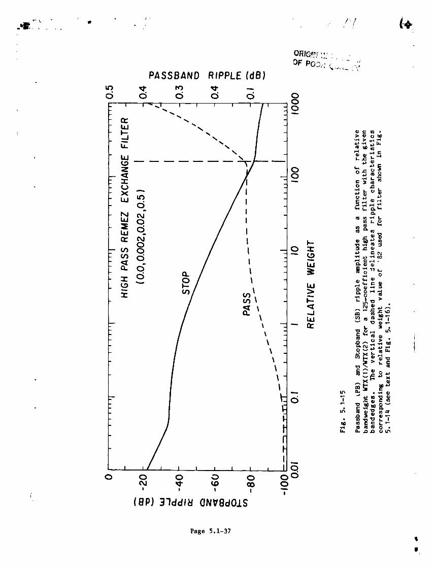
_age 5.1-37i
i
1984026903-066
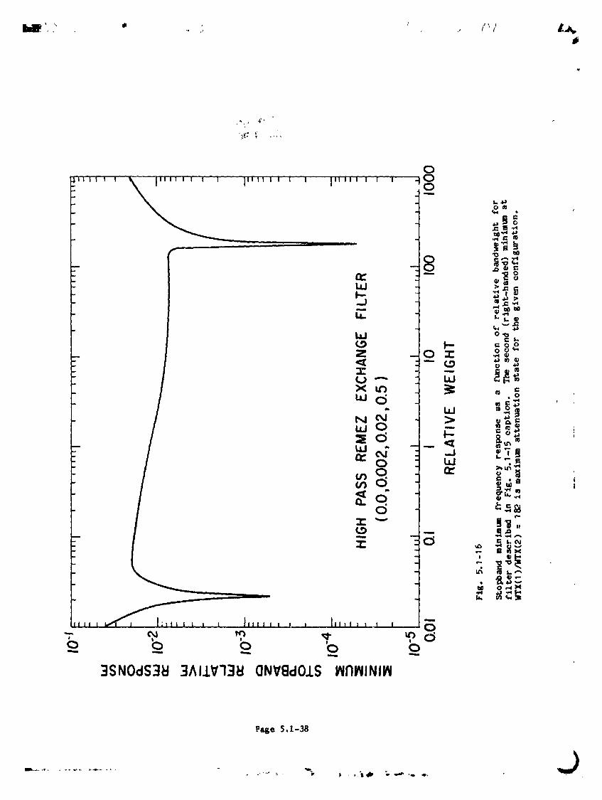
0
"_'1111 I ....... li1111 r'i ....I ' IlUUUU U U U ,0 0
..- ,, _._
P _
. Z -0 Z _®
w c; I 0
. .__.,_ ,
uuO > _
o _ _ ,°.: ,
Z _ _ .__ _^
' _0 ,,,,_P'<
.,-,
b '0
3SNOdS3_ 3AIIV73t:l (]NVBdOIS RI'IlNINIIN
Pase 5.1-38
1984026903-067
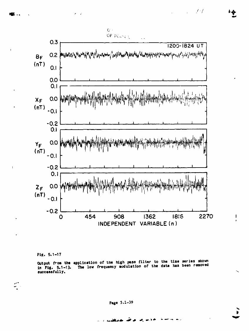
t*.
OF i;C,_':_ '.....
0.3 1200- 18,24 U TI
02
(nT) 0.1 t0.0 L , , I I , , . I J "0.1 --
x,oo(nT) -0.1
-0.2 I n L , n I I , a J
0.1
YF 0.0 _'I(nT)-0.I -
-0.2 ' I I I _ I. , 1 ,0.1 - '
(nT)-0.1 _"
-0.2 , i i i i . , .... i , I . ,• 0 454 908 1362 1816 2270' I
P
INDEPENDENT VARIABLE (n)
Ftl;, 5.1-17
Output _om the application of the hlsh pa88 £11tar to the time serlel ahotmIn Fii. 5.1-13. The Zow frequency IodulmtLon o£ the data has been removedsuoeeaatully. \
w_
?a_e 5.1-39
i
., , _.'iI_dI_-_.*_ ,,. o.'s_ ;.-".- .,... V
1984026903-068
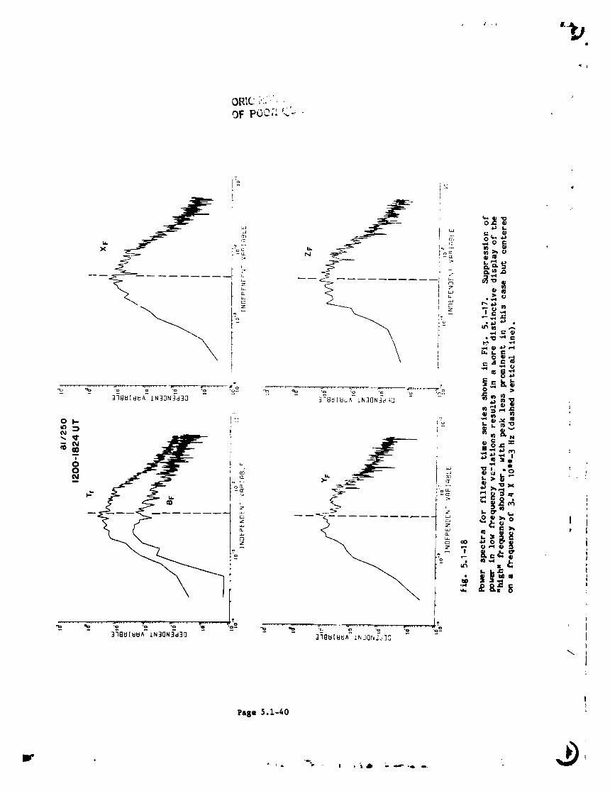
I
/
j__1 kJ
crJ _ O0 I_
i'o L_- .
_ ,,,_
t " ! _='T"_D
co ,,_ ,,,,az;," ipz _ e,,,I o _ll
'o _ 7
!:. ,2............................................_ '° '° '° %-........ _-'% _........" '_.......... "-/"'_"' _' ..................' '° '° '-37BUI_U^ 1N30N3d30 3_SU[w_^ 1NJOt_Jj70
!
[,,,Be 5.1-40
1984026903-069

'] -I.O . I i II.0 i _ -r i i
I
o 0
liiii!iiii' 1!.0i_:i_:;i., i i , I.i:i:iiiii::l
-J 17iUA
i 0 i it 0 .002 .004 .006 .003 .010
4"
INDEPENDENT VARIABLE (Hz)
/i Fig. 5. 1-19,i
! Etgenfunetion properties of the fluet, uations shoun in Fig. 5.1-17 in thefrequency band 0.001 to 0.01 HZo Parameters plotted _re same as those _n Fig.
i 5.1-.11. Frequency of perk power in the fluctuations is delineated by the, vertical hatched band. Comparison with Fig. 5.1-11 shows properties or waves
at 3. q X 1On- 3 Hz are similar to those of the 1.75 X 10ii-4 Hz waves.
£age 5.1-41
1984026903-070

5.2) DIGITAL FILTERS (OPERATORS FILDES, FILOPT, FILTER AND WTS)
" 5.2.1) INTRODUCTION TO DIGITAL FILTER DESIGN USING REMEZ EXCHANGE
Built into IDSP are operators that allow a user to degign nonrecurslve Finite
Impulse Response (FIR) digital filters and then apply these filters to the
time series. There is currently no capability to design Infinite Impulse
Response (IIR) filters in IDSP.
Nonrecursive FIR filters have the following properties:
1) They are implemented in a nonrecurslve fashion (operator FILTER),i.e., there is no feedback in the equation, (thus the name "Finlte";IIR filters must be implemented recursively).
2) Because of property (I) above, they are always stable. On the otherhand the stability of IIR filters must always be checked.
3) They can be made to be linear phase operations, i.e., with zero phasedistortion, by making the number, N, of filter coefficients odd and
centering about sample number (N-I)/2. IIR filters are not of linearphase.
4) They are straightforward to design (operators FILOPT and FILDES).
5) FIR filters are not as efficient as IIR filter, i.e., for given
design specifications IIR will require fewer multiplications. Thisefficiency can be important when large quantities of data are to befiltered and/or the filter has a large number of coefficients, or inthe case where the filter is to be implemented in hardware. However,
in IDSP these considerations are usually not important, so only FIRdesign is provided.
The FILOPT and FILDES operators use a computer program developed by McClellan,
Parks and" Rabiner (see Rablner and Gold, 1975) that employs an algorlthm
c_lled Eemez exchange which is very efficient in producing an optimal (in the
weighted Chebyshev sense) filter. This program has found wide application in
the area of digital filtering and is considered state-of-the-art. The
original program was obtainzd from the IEEE Library of Programs for Digital
Signal Processing (see Programs for Digital Signal Processing, 1979) and
restructured as operators for use in ID6P.
Before illustrating the use of these operators, we introduce the concept of
normalized frequency: NORMALIZED FREQUENCY=(ACTUAL FREQUENCY)/(SAHPLE RATE),
wlth units of cycles per sample. Thus the Nyqulst frequency will always be
0.5 in normalized Hz. As an example, if we sample a 20 Hz signal 100
tlmes/sec the normalized frequency is 0.2 Hz.
Page 5.2-I
section 5.2 5125184
.°. #
1984026903-071
w
!
The important filter design speciflcatlons are shown in Fig. 5.2-I (see
"_ Schaff, 1979) where the abscissa is plotted as normalized frequency.
i
._ [O,fp] is the normalized PASSBAND
[f ,fs] is the normalized transition width, delta FP
_r [fs,O.5] is the normalized STOPBAND
delta I is defined as the amplitude deviation in the PASSBAND
_ delta2 is defined as the amplitude deviation in the STOPBAND
PASSBAND RIPPLE is defined to be 201og10(1+deltal) in dB
STOPBAND RIPPLE is defined to be -201og10(delta 2) in dB
I
Typical values for the PASSBAND RIPPLE would be in the range of I to 0.01 dB
and for the STOPBAND RIPPLE 20 to 90 dB.
5.2.2) DESIGN OF BANDPASS/BANDSTOP FILTERS
The following example illustrates how to go about designing a filter and in
turn applying it to the time series. (_, the Dynamics Explorer Spacecraft
_ there is a magnetic field experiment that provides a vector measurement of the
ambient magnetic field every 0.5 sec. The data from one of the components of
the vector is shown in Fig. 5.2-2 as a function of time. As is evident there
appears to be a substantial periodic signal riding on top of the actual s_gnal
of interest. It was desired to remove this contamination from the signal of
interest. First it was necessary to do s spectrum analysis on the data to
determine the frequency(s) of the unwanted signals present in the data.
Fig 5.2-3 shows the results of using operators WINDOW, FFT, SPECT and GRAPH
I on this time series; note that at 0.0324 and 0.175 Hz there are peaks in the
j spectrum resulting from the unwanted signals.
7i The first order of business is to design a FIR filter to remove the unwanted0.0324 Hz signal (0.0162 normalized Hz, e.g., 0.0324/2).
Page 5.2-2
section 5.2 5/25/8qJ
..)"
1984026903-072

/'. !
Referring to Fig. 5.2-I, once the designer has decided on the number of filter
coefficients and the normalized transition width for a particular filter
design the important parameters are I + delta I (the bandpass ripple) and
delta2 (the bandstop ripple) as a function of the weight ratio, deltalldelta 2
= WTX(1)/WTX(2) (see Rabiner and Gold, 1975, pp 197,199). Delta2 is a measure
of how successfully we will attenuate the unwanted part of the frequency
spectrum and we want to make this value as small as possible, while at the
s_me time minimizing the bandpass ripple, I + delta I. In order to aid in
making the necessary tradeoff decisions we have developed an operator, FILOPT,
which computes, using the Remez exchange algorithm, the values, in dB, for I +
delta I and delta2 over a range of deltalldelta 2 ratios• Typically operator
FILOPT (see Section 6) would be used to compute I + delta I and delta2 over 4
decades of the ratio (from 0.1 to 1000). Because it is necessary to execute
the Remez exchange algorithm over such a wide range of ratios it was decided
to only do the computation for 9 values each decade and use operator INTERP to
interpolate for the equidistant spacing required by IDSP. This dramatically-[
decreases the amount of computation time required to execute FILOPT. Ther.
_I operator FILOPT produces an IDSP compatible data set consisting of elements of
; three time series for each weight ratio (see Fig. 5.2-4): series I = passbandi
i ripple = 201og(1_deltal); series 2 = stopband ripple = 201og(delta2); and
" series 3 = the minimum value of delta 2 in the stopband. It is then necessary
for the designer to interpolate (operator INTERP) data set FILOPT so as to
produce the data set, INTERP, that can then be graphically displayed using
operator GRAPH. The designer can then use these graphs to make a decision
about what weight ratio will give the best stopband attenuation for the
minimum of passband ripple.
Another approach, if there is some flexibility in the number of filter
- coefficients that can be used, and the designer wishes to prespecify the
values for delta 1, delta2 and the transition width is to estimate the number
"_- of filter coefficients from the following empirical formula which is valid for
lowpass filters and has been implemented as operator WTS (see Section 6).
Page 5.2-3
section 5.2 5125/84
1984026903-073

NFILT • D(deltal,delta2)/(delta F) - £(deltal,delta2)(delta F) + 1.0
delta F = ABS(fs-f p)/
D(deltel,delt: 2) [al(lOllodeltal) 2 �a21oglodelta1 + a3]lOglodelta 2
+[a_(lOglodeltal) 2 + a51Oglodelta 1 + a6]
f(deltal,delta _) = b_ + b:(lOglndelta 1 - logtndelte _)
.r, 30,x,03; ,,,ilO2;;3.-,:761xi'; 266;;0 ;5:59,,x,0aG:-q.278110-1; b1=11.01217; b2=O.512qq
In our case we used FILOPT to determine the best tradeoff for delta 1 and
delta 2. For this filter we decided to use lq9 coefficients; £p = 0.0055 and£ : 0.0155 for the first transition width and £ = 0.017 and £ = 0.027 fors s pthe second transition width, We then use FILOPT to provide us with guidance
on _hat is the best tradeof£ for delta 1 and delta 2, Referring to the output
o£ FILOPT shown in Fig. 5.2-q we conclude that a ratio o£ W_X(1)/WTX(2) = 2.5
gives us small bandpass ripple and acceptable bandstop characteristics. We
nok have all of the design specifications for this first filter and can set up
specifications to allow operator FILDES to be used to design the desired
filter.
To do this we generate a data set on disk that has the following format:
First record: NFILT,JTYPE,NBANDS,LGRID. (qI5 format)
Next record(s): EDGE (4F15.9 format)
Next record(s): FX (qF15.9 format)
Next record(s): WTX (4F15.9 format)
These records can be placed into [usrtd. I_6P]FORO58.DAT or a data set o£
another name, if the user does not want to enter design specifications
Interaotlvely. In general it is probably better to generate the data set for
purposes of documenting the design rather than entering them interactlvely.
NFILT-- FILTER LENGTH;
JTYPE-- TYPE OF FILTER
1 : MULTIPLE PASSBAND/STOPBANDFILTER,
2 : DIFFERENTIATOR,
3 z HILBERT TRANSFORMFILTER;
Psse 5.2-4
section 5.2 5/25/8q
1984026903-074
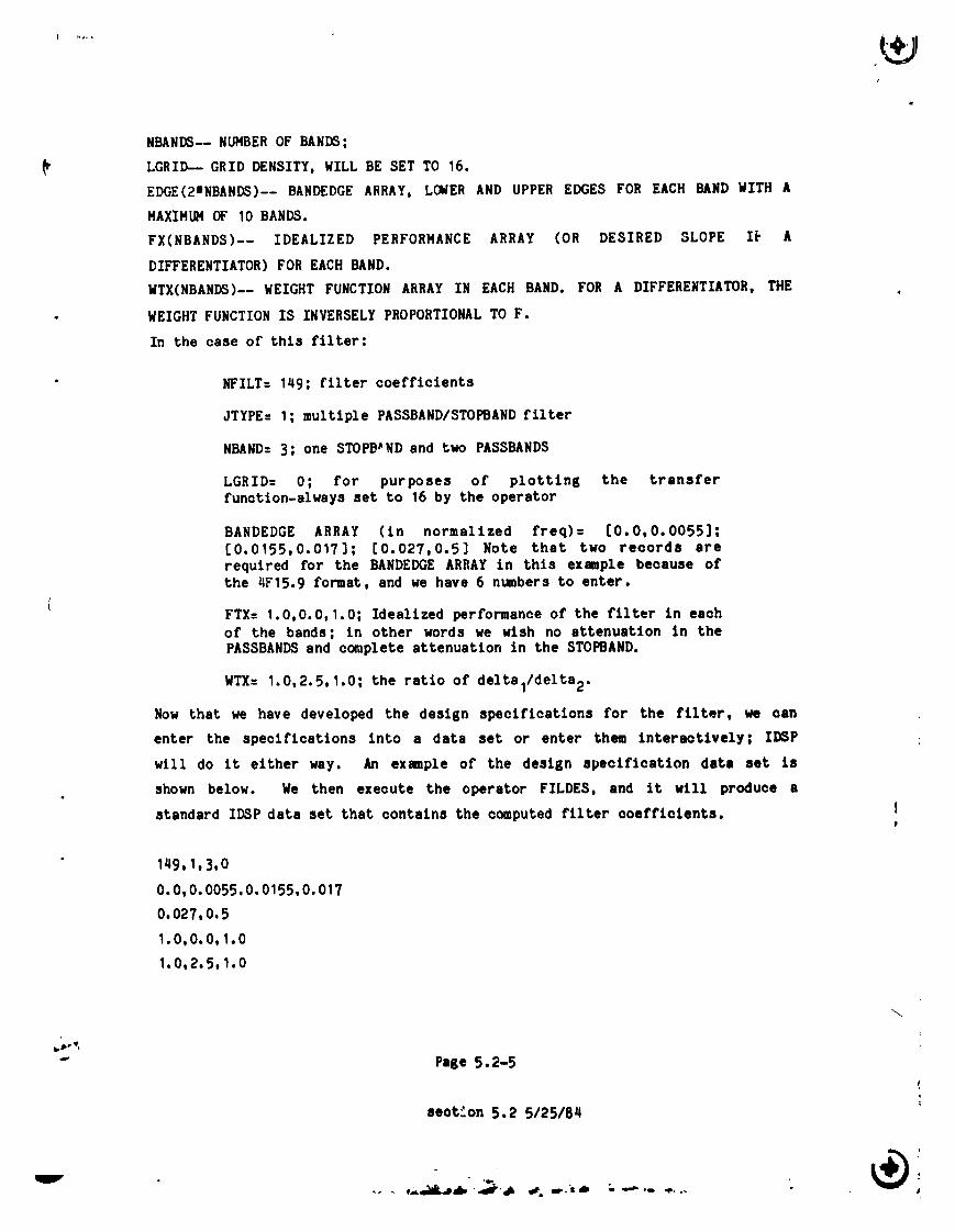
/
NBANDS-- NUMBER OF BANDS;
_- LGRID-- GRID DENSITY, WILL BE SET TO 16.
EDGE(2mNBANDS)-- BANDEDGE ARRAY, LOWER AND UPPER EDGES FOB EACH BAND WITH A
MAXIMUM OF 10 BANDS.
FX(NBANDS)-- IDEALIZED PERFORMANCE ARRAY (OR DESIRED SLOPE I_ A
DIFFERENTIATOR) FOR EACH BAND.
WTX(NBANDS)-- WEIGHT FUNCTION ARRAY IN EACH BAND. FOR A DIFFERENTIATOR, THE
WEIGHT FUNCTION IS INVERSELY PROPORTIONAL TO F.
In the case of this filter:
NFILT= 149; filter coefficients
JTYPE: I; multiple PASSBAND/STOPBAND filter
NBAND: 3; one STOPB_ND and two PASSBANDS
LGRID: O; for purposes of plotting the transferfunction-always set to 16 by the operator
BANDEDGE ARRAY (in normalized freq) = [0.0,0.0055];
[0.0155,0.017]; [0.027,0.5] Note that two records are
required for the BANDEDGE ARRAY in this example because ofthe 4F15.9 format, and we have 6 numbers to enter.
( FTX= 1.O,0.0,1.0; Idealized performance of the filter in eachof the bands; in other words we wish no attenuation in thePASSBANDS and complete attenuation in the STOI_AND.
WTX= 1.0,2.5, 1.0; the ratio of deltal/delta 2.
Now that we have developed the design specifications for the filter, we can
enter the specifications into a data set or enter them lnteractlvely; IDSP
will do it either way. An example of the design specification data set is
shown below. We then execute the operator FILDES, and it will produce a
standard IDSP data set that contains the computed filter coefficients, t
149, I, 3,0
O. O, O. 0055, O. 0155. O, 017
O.027, O.5
1.0,0.0, 1.0
1.0,2.5,1.0
k, Jb"
" Page 5.2-5
section 5.2 5/25/84
,.. ,_bl_db _e'ab =e f'= d* . .._,. _ .. _m_ A
1984026903-075
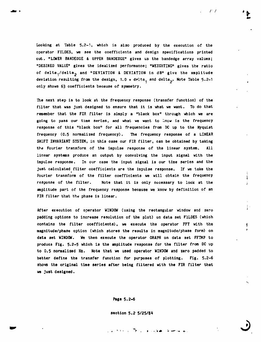
Looking at Table 5.2-!, which is also produced by the execution of the
operator FILDES, we see the coefficients and design specifications printed
out. "LONER BANDEDGE & UPPER BANDEDGE" gives us the bandedge array values;
"DESIRED VALUE" gives the idealized performance; "WEIGHTING" gives the ratio
of deltalldelta 2 and "DEVIATION & DEVIATION in dB" glve the amplitude
deviation resulting from the design, 1.0 + d_Ite I and delta2. Note Table 5.2-I
only shows 63 coefficients because of symmetry.
The next step is to look at the frequency response (transfer function) of the
filter that was Just designed to ensure that it is what we want. To do that
remember that the FIR fllter is simply a "black box" through which we are
going to pass our tlme series, and what we want to ::now is the frequency
response of this "black box" for all frequencies from IX: up to the Nyquist
frequency (0.5 normalized frequency). The frequency response of a LINEAR
SH]FT INVARIANT SYSTEM, in this case our FIR filter, can be obtained by taking
the Fourier transform of the impulse response of the llnear system. All
llnear systems produce an output by eonvolvlng the input slgnal with the
impulse response. In our case the input signal Is our tlme series and the
Just calculated fllter coefficients are the impulse response. If we take the
Fourier transform of the filter coefficients we wlll obtain the frequency
response of the filter. Note that It is only necessary to look at the
amplltude part of the frequency response because we know by definition of an
FIR filter that the phase is linear.
J
After execution of operator WINDOW (using the rectangular window and zero
padding options to increase resolution of the plot) on data set FILDES (which
contains the filter coefficients), we execute the operator FFT wlth the l
magnitude/phase option (which stores the results in magnltude/phase form) on
data set WINDOW. We then execute the operator GRAPH on data set FFTNP to
produce Fig. 5.2-5 which is the mplttude response for the filter from DC up
to 0,5 normalized Hz. Note that we used operator WINDOWand zero padded to
better define the transfer function for purposes of plotting. Fig. 5.2-6
shows the original tlme series after being filtered with the FIR fllter that
we Just designed.
Page 5.2-6
section 5.2 5/25t8_
I
1984026903-076
LZ.J
In a similar fashion we design the second filter, again using FILOPT to
determine the optimal design, to remove the unwanted 0.175 Hz (or 0.08?5
normalized Hz) signal. The amplitude response of this second filter is shown
in Fig 5.2-7. The design specification data set appears below:
125, 1,3,0
0.0, 0.05,0.075,0.1
O. 125,0.5
1.0,0.0,1.0
• I.0,38.O,1.0
Finally, we filter the time series a second time to remove the 0.175 Hz signal
and the resulting tlme series is shown in FIg. 5.2-8, substantially free of
both unwanted signals.
It should be noted that for purposes of illustration we have designed two
separate filters; however, both unwanted frequencies could have been removed
with a slngle filter that has two stopbands and three passbands for a total of
i 5 bands. Operator FILOPT and FILDES will permit you to design a filter with
up to a total of 10 bands and 512 coefficients, it
The design tradeoff information of this 5 band filter from FILOPT is shown in
FIg. 5.2-9. The transfer function is shown in Fig. 5.2-I0 where a i
deltal/delta2= 8.0 was chosen as optimal. Table 2.0-! results from the
execution of operator FILDES and presents the coefficients and other '
parameters of this 5 band filter. Fig. 5.2-11 shows the results of filtering
the original tlme series from Fig. 5.2-2 with this filter. Fig. 5.2-12 showsI
the power spectrum of thls filtered data processed with the 5-band filter;
Fig. 5.2-13 is the power spectrum of the data set filtered with the two 3-band
filter. In both cases the contaimlnation signals have been removed.
Fig. 5.2-21 depicts the _erles of operations involved in the optimal design o;
a multiple band filter using IDSP.
. m"
Page 5.2-7
section 5.2 5/25/8q
A
i
1984026903-077
•JIB! .... / /!
5.2.3) USE OF A DIFFERENTIATING FILTER:
The spectral analysis of a finite duration time series nay Include errors due
to "leaksge'. This error is most likely to modify regions of the spectrum
' which contain little power by leaking power from more energetic frequencies,
through the influence of the side lobes of the data window (see Section 5.3
for a detail discussion of windows) used in the analysis. One way to
determine if a particular spectral feature Js real or due to leakage is to
"pre-whiten" the series using a differentiating filter. In effect this
multiplies the original spectrum by the "one" power of the frequency (F) which
amplifies the high frequency relative to the low. For spectra which are
dominated by low frequency power, the differentiator flattens, or nwhttene"
the spectrum aed decreases the leakage effect on high frequency spectral
features •
As an exmtple of designin8 a differentiating filter consider the tangential
(T) and normal (N) components of a aagneti - field vector plotted as a function
of time in Fig 5.2-14 and Fig. _,2-15, respectively. Fig 5.2-16 shows the-5/3
power spectrum of this vector. This spectrum decreusee at approxtmatel7 F
for large F, so that spectral features in the higher F region may be/
influenced by leakage from the lower F region.
A differentiating filter was designed using the operator FIT,E2 to prewhiten
these data. This filter is 126 coefficients in length with a cutoff frequency
at 0.5 and a slope of 1. The design specification data s t is as follows:
126,2,1,16
0.0,0.51
1.0
1.0
The filter coefficients are shown in Table 5.2-2, and the _ransfer function is
plotted in Fig. 5.2-17 The filtered versions of T and N are shown in Fi8.
5.2-18 end 5.2-19, respectively. The low frequency features are visibly
absent, and the data appear to be mu_,h more like white noise. This is borne
out by the power spectrum sho_ in Fig. 5.2-20 which is now flat at large F.
Page 5.2-8
section 5.2 5/31/84
1984026903-078

QJ
w
REFERENCES
Programs for Digital Sl_nal Processing, IEEE Press, 1979.
Rablner, L. R., B. Gold, Theory and Appllcstlon of Digital Slgnal Processing,Prentice-Hall Inc., Englewood Cliffs, N J, 1975.
Schaff, W. E., Course Notes: Modern Methods of Digital Sl_nal Processing,
, Integrated Computer Systems, Ino, October 1979.
i
!a
I
Page5.2-9
section 5.2 5/23/8q
tv _
1984026903-079
OF POOR(,IUALI<
I
.... ,............ , .............. ,........... __ .
®®®®®®®®®®®®®®???_??I/lllllllllllll I ¢__¢__
II II n II II il II ii II li II ii II l® li ,1 ii il ii ii ,I i, _® _ i # _ I ® _ I ® _ _ ® _ _
°=oo°.oooo.oo.oooo11 "O00"mO0=+'+'''O0
_illlllllllilllll i
i _ II II II II ii II 11 II II II II II Ii II II II II ii II II II II Ii II II II II n II II II It II n ii ii ii ii ii ii ii ii ii ii ii ii ii ii ii ii #1 ii ii
_ ® ®® ® ®® ® ® ®@®® ® ® ®_
_ II II u it II II n II li II II II II II II II II Ii ii II II it il n ii ii n II ii ii ii ii II It it II II ii ii ii ii II ii ii ii ii II Ii ii ii ii II I
iiiiiiiiiiiiiiiiiiiiiii 1111111....... iiiiiiiiiiiiitliiiiiiii
Page 5.2-10
!,
1984026903-080
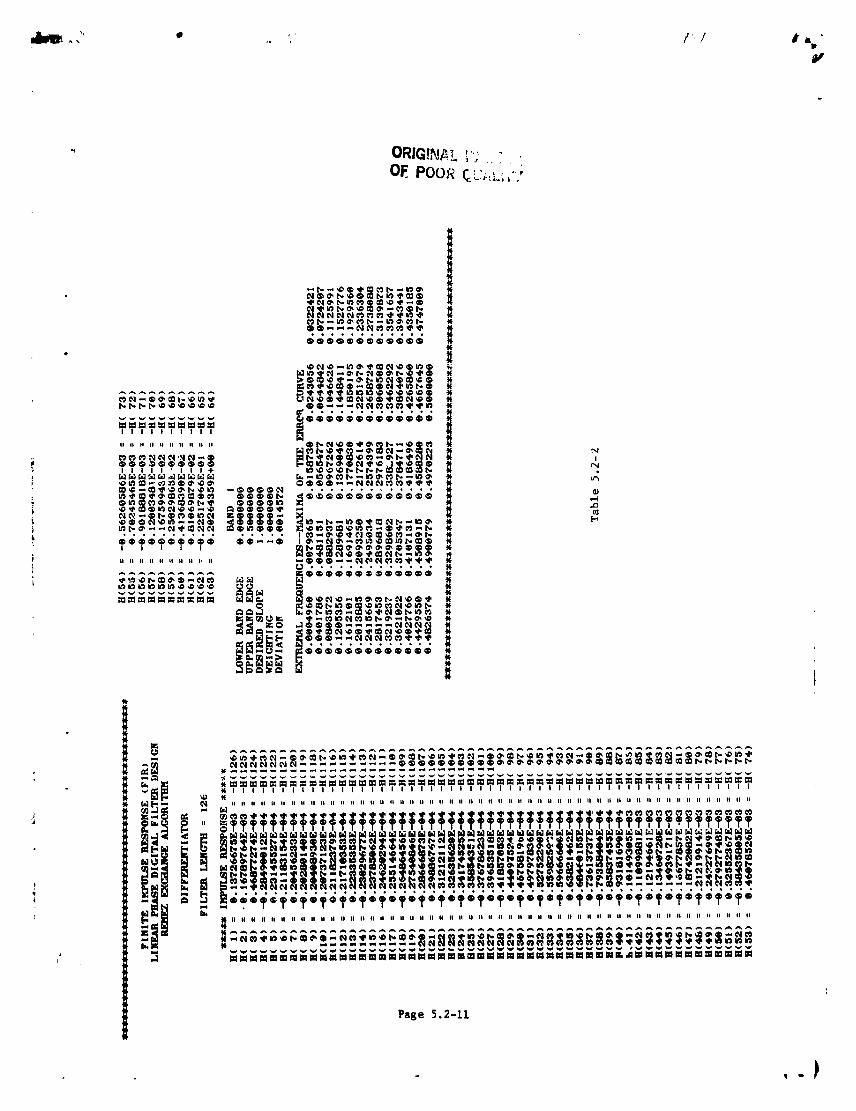
OF PO0_ _. _,,
8
• _
i _'''''=" ..... *
_i °°°°°°""......."'""="'°°'°_'°°_'===°'"'°'__--• 3 " ._3..3ZZ3Z3Z'3Z''Z33Z'"i ::::::::::::::::::::::::::::::::::::::::::::::::::::::
_ _l|ililllll lili, lilll! llilil liiliil ilillli Ill= _ _ " ........ ,................... ,, ............. , .... ,,,, ....... ,,,,, .... ,,,, ,,,,,, ,,,, ............. , ..... , ,,
****,,_,,,,****o,,******,,,*,*********°_''****'**_°''
®®®?_?®?®?_?®?®?®?®?®?®?®?®?®_®?®?®?®?®?®?®_®?®?®?®?®
=-
Page5.2-11
1984026903-081
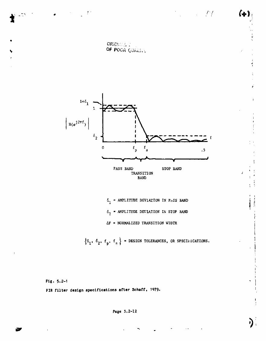
41
OF POOi_ QJAL; ,,.
1+611
IH(eJ2_f) II
62 I .... f
0 f fp s .5
"- _ ' _4 e
PASS BAND STOP BAND , ,
TRANSITIONBAND
= AMPLITUDE DEVIATION IN PASS BAND
_2 = AMPLITUDE DEVIATION IN STOP BAND ii
AF = NORMALIZED TRANSITION WIDTH 1
L
, f = DESIGN TOLERANCES, OR SPECI_ZCATIONS.
FiB. 5.2-1
FIR filter destzn 8peotfioatton8 after _haf£, lq79.
Pase 5.2-12
1984026903-082
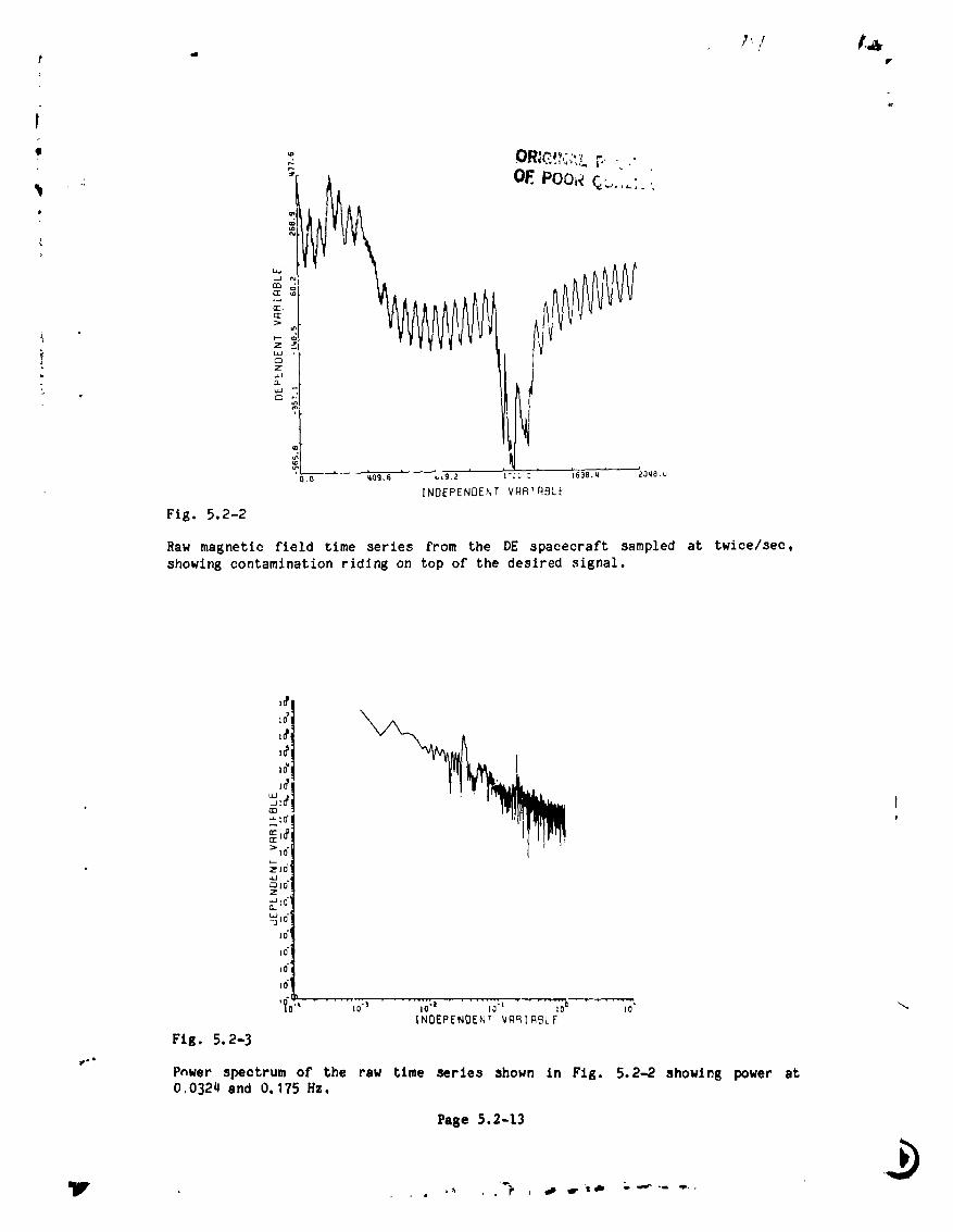
I I f.,__ , Y
f
L
•Z
.
I0.0 _09.6 _,9.2 l-;; : J638.q
INOEPENDENT VNR'ABLL
Fig. 5.2-2
Raw magnetic field time series from the DE spacecraft sampled at twice/see,
showing contamination rldlng on top of the desired signal.
l#
I@!
i@
CD
>16ZIO
s_ IO
%,di0"q
10"
16'
INOEPENOENTVARIABLE
Ft8. 5.2-3
Pnwer spectrum o£ the raw tlme aeries shown in Fig. 5.2-2 showing power at0,0324 and 0.175 Hz.
Page 5.2-13
._ .'-_ ,i, ,,';" :'-"'" ""'
1984026903-083
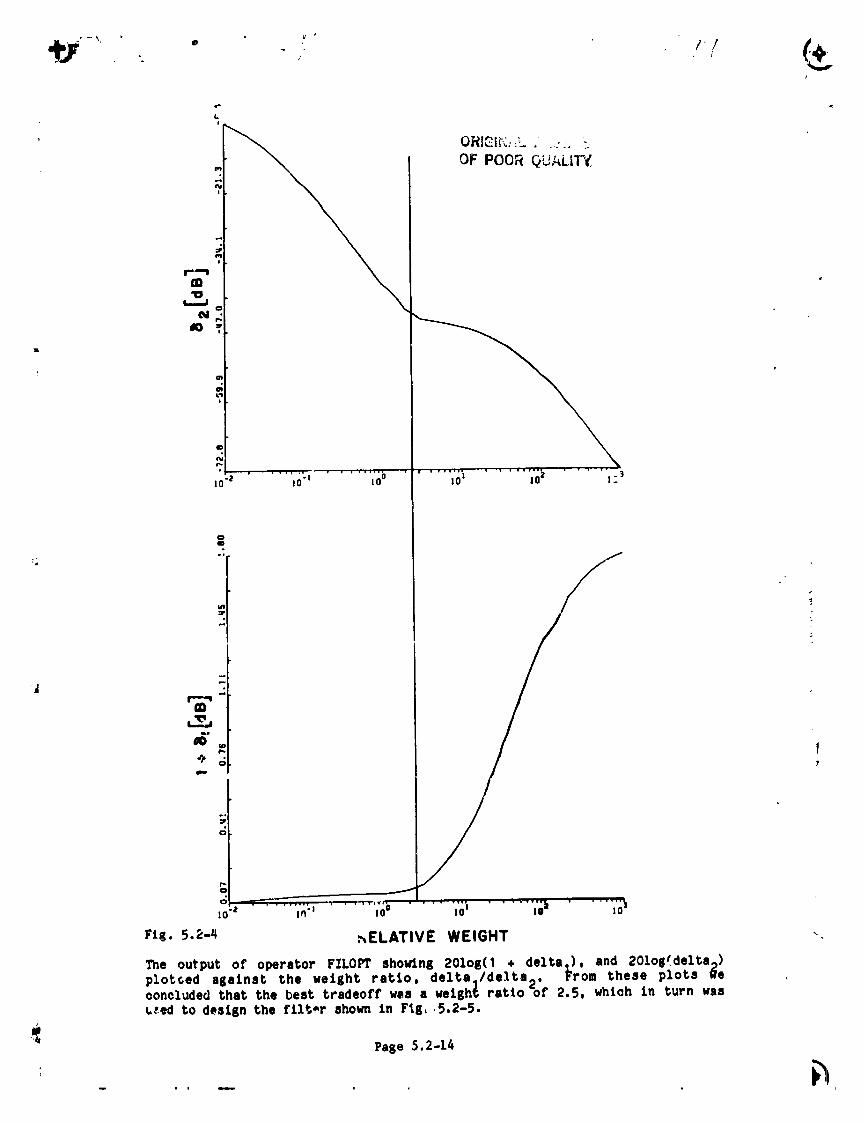
OF POOR _U/-_L,IT'I(
g
"0
¶
i0-_ i0 "l i0 ° i01 10 _ 1 _
QI
_ I
1o" ,_" _'(o° ,o' "'iP ",'o_Fig. 5.2-_ ,_ELATIVE WEIGHT "
The output at operator FILOPT showing 201og(1 + delta1), and 201og(delta_)plotted aKainat the ueiiht ratio, deltal/delta 2. From the_e plots geoonoluded that the bent tradeoff waa a wetgh_ ratio of 2.5, whioh in turn waau,,.ed to design the ttlt,r ahoun in Fig, ,5.2-5.
Page 5.2-14
1984026903-084
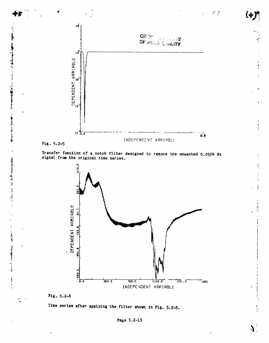
Id:"_ • q_
Ii OR;.T_".. -.,N '",,: OF VC__,-.:_..;ALI'h(.
P"_ ° /
i w ;!N ' !d CI: " '
g _,,j .
"" O- "
i ,$
IO-L _ , i .... i i I A i - --_.J
"_ o.o 0.5] NDEPENDE_.NT VARIABLE
Fig. 5.2-5
Transfer function of a notch filter designed to remove the unwanted 0.0324 Hz
signal from the original time series.!
:}. ;I
,°
i
! '•4 r_1 _, .......Lo '3eo.o '_6o.o ' 'n,_o.o _2.,.o 19oc
INDEPENDENT VRRIRBLE
Fig. 5.2-6
Time series after applying the filter shorn in Fig, 5.2-5.
Pa&e 5.2-15
1984026903-085

_= tO 0.00 0.|0 0.20 O. JO O,qO 0.50
INDEPENOENT VRRIRBLE
Fig. 5.2-7
" Transfer function of a notoh filter designed to remove the unwanted 0.175 Nzsignal from the tlme series.
\
Z
Z
?
INDEPENDENT VRRIRBLE
Fig. 5.2-8
Time series after appltcattc, n of both the filter sho_ in Fig. 5.2-5 and Fig.5.2-7. Note that the time series is substantially free of the unwantedsignals.
Page 5.2-16
"1 I
1984026903-086

lID
N410
II0"z I !0 zm
o
o
m
+o
.....;;b ,o' ......;o_ " 'i;_
Fig. 5.2-9 RELATIVE WEIGHT \
The output of operator FILOPT showtn8 201o8(1 , delta1), and 20los(delta o)
I... plotted asatnst the weisht ratio, deltal/delta 2. From these plots (_econcluded that the best tradeoff was a weisht ratio of 8, which in turn was
used to deslgn the filter shown In FIB. 5.2-10.
Page 5.2-17
1984026903-087

io-
d:oo ' 6 ,o _ 20 6.30 ' 6.40 ' '. • 0.5
INDEPENDENT VARIABLEr Fig. 5.2-10
The transfer function of the 5 band filter is shown. This transfer functionis obtained by using operator FFT on data set WINDOW which contains the filtercoefficients.
Ill I *r7
_ t_
i
/
1
',d
0.0 359.6 719.c 1070.8 1_38.q 1790I NDEPLN[1ENT VQR] ABI.E
Fig, 5,2-11
Shows the results of using operator FILTER to filter the original tlme sevlesshown in Fig. 5,2-2 with the 5 band filter shown in Fig. 5,2-10.
Page 5,2-18
),
1984026903-088
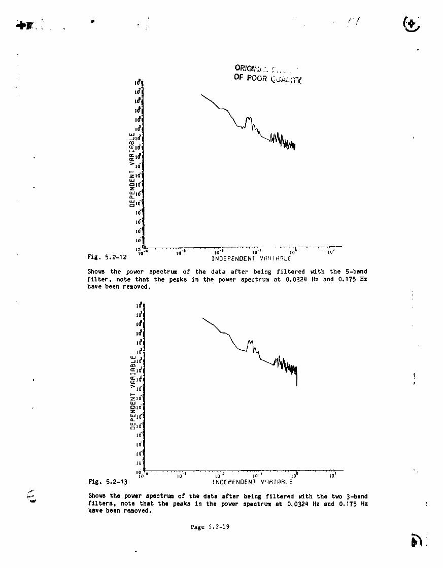
ORIG_b _,, _,• a, ....
I#I OF POOR £.J,kLl'i-_,,,,'i
_o"_,o"zw!6IL
N,o-!
lff'
16_
t6 _! , , ,-,,,, ...... --_ r_ .... -rTT,V ----"T- ,_l--_
1_0. q ' |0.._ " • , |0. 2 _10"1 i0 u lO !
Fig. 5.2-12 INDEPENDENT V_IRIflRLE
Shows the power spectrum of the data after being filtered wlth the 5-band
filter, note that the peaks in the power spectrum at 0.0324 Hz and 0.175 Hzhave been removed.
I¢I,o'i
,o'i _X_
_o'• _ao° !
>16 t P
P__,ol,o-i
t6
,oi,oi
I IO'O'q ' I0 "l |0 _ I0 I i0 I
Fig. 5.2-13 INDEPENDENT vqRIFIBLE
,j"
r- Shows the power spectrum of the data after being filtered wlth the two 3-band
filters, note that the peaks in the power spectrum at 0,032_1 Hz and 0.175 Hz thave been removed.
Page .5.2-19
1984026903-089
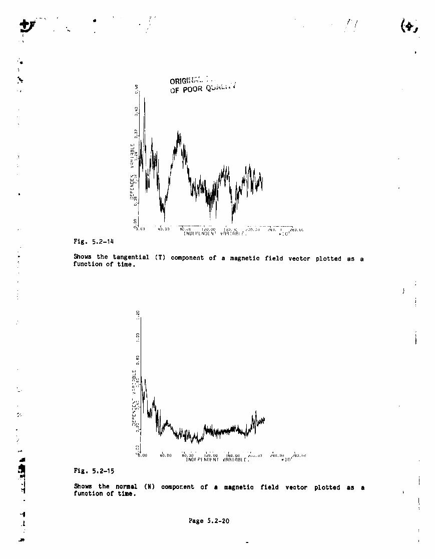
+j' .. " ' .", ,,'I (+,I
"Q.
I.
,. ORIGI,........OF pOOR QbP.L;,;; o"
uJ
crfu
¢dF
z_ I
zL_ILL
• LLIoN
o"
• - [JO 40.00 80.dO IdO.O0 160.UO dOO.O(J 2i_0. L) 2gO.DO
[N[3_-P[NOfNI VnR[NBt [. _!0 L
Fig. 5.2-1q
• Shows the tangential (T) component of a magnetic field vector plotted as afunctionof time.
4
LCJ.J
i ell _
Irl"
uIll
n_
/
I ,_t), Or) 160,00 eL+,,, till _4t). 280, till
.__ INDFPINDFNI _/ARIABI[. .10'Fig. 5.2-15
=_
._ Shows the normal (N) componentof a masnetic field vector plotted as afunction of time.
.t_[ Page 5.2-20
1984026903-090

W
l
't
ORIG!_; _ C,
: '#I OF POOR QU:: Y ,
" _1o"
:i " '°ILI 10
I01 i0 ;_ i01 IU _
INDFPFNN_-NI" vn_inI4, _ .
"i Fig. 5.2-I 6i
Shows the F_wer spectrum of the magnetic field vector plotted in Fig. 5.2-14and 5.2-15.
,5 g
Ij_
CE
zI LLJ
C-1
ill
,/, /
o. o 3_,g-............ os.o 57. _ ................. s,_.4 6_.o
]NOFP_NDENT VnnlnBt E
Fig. 5.2-17 \
Shows the transfer Cunetlon of the differentiating fllttr..!
Page 5.2-21
1984026903-091

IRBLE.INDEPENOENIVRR
Fig. 5, 2-18
Filtered version of T originally piotted in Fig, 5.2-14,
. 4
|
t
: "rg
• 1
g
-I
!
-] 'moo - ,_o.oo- _--ou _)o ou 3bmoo"" aoo.oo_........... a_o,oo_--- " Juo.oo'; INO(PENIJE'NI V_IABLE, _lO_
Fig, 5.2-19
Filtered version o£ N originally plotted in Fig. 5,2-15.
Page 5.2-22
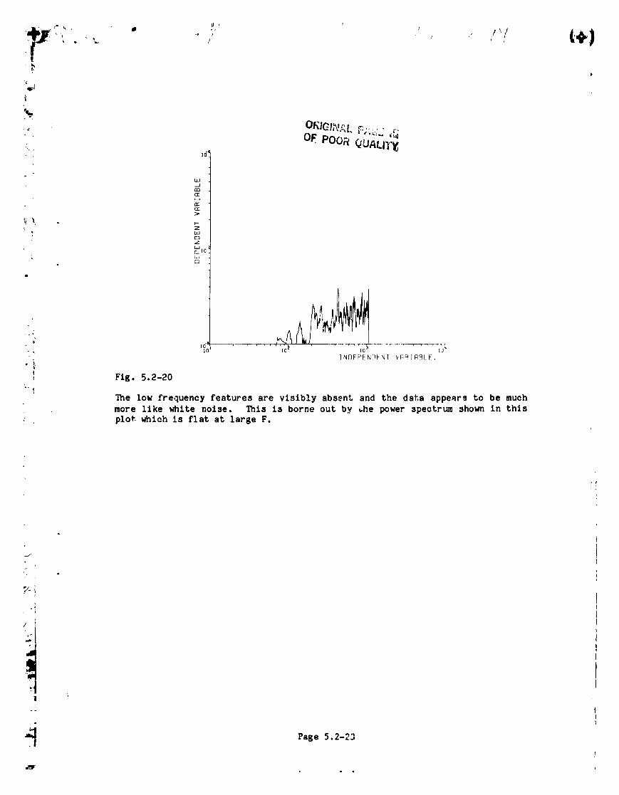
'_ . , _ J ,. . ,
I,
%., OKIGII'_,.fil ,-.. ,
OF PO0_ (_UALi_<_:,, , io-(
uJ==J
n-
CC¢Iz
, 7.z
tiJc3
e
]NDFPEN[_I- NI VN_ I RBL [.,
Fig. 5.2-20I
The low frequency features are visibly absent and the data appears to be muchmore like white noise. This is borne out by the power spectrum shown in thlsplof. which is flat at large F.
1
-" t
_1 Page 5.2-23
l
1984026903-093
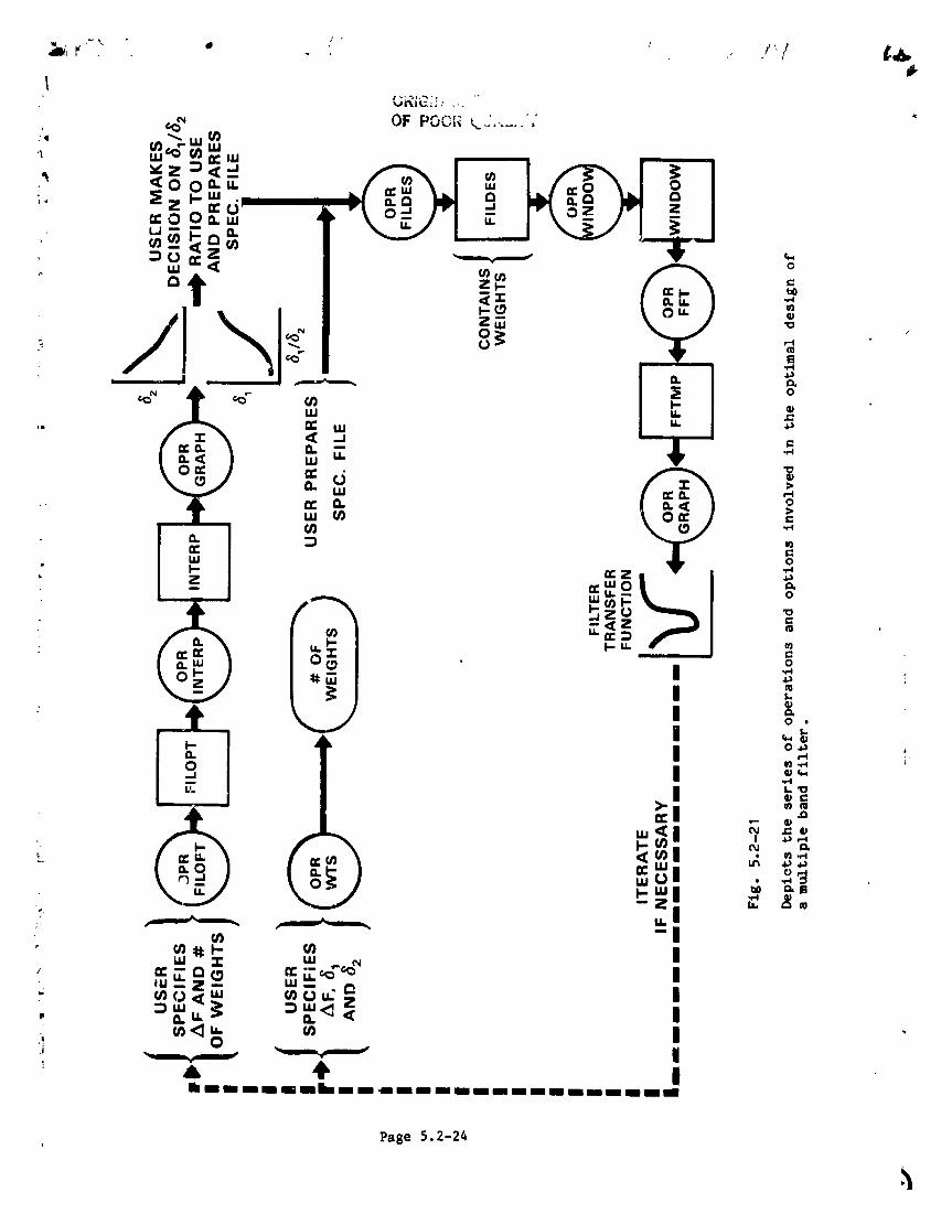
Page 5.2-24
1984026903-094

5.3) THE EFFECT OF WINDOWING_ ZERO PADDING, AND OBSERVATION TIME ON THEESTIMATION OF SPECTRA OF SINUSOIDS (OPERATORS SETUP. WINDOW, FFT. ANDSPECT)
There are two fundamental issues in estimating spectra (see operators WINDOW,FFT, AND SPECT) of slnusoids:
Resolution- How close in frequency can multiple sinusoids be spaced andstill be uniquely identified in the spectrum.
Dynamic Rand_e- How large can the differences in amplitudes of thesinusoids be and still be uniquely identified in the spectrum.
The choice of the weighting function (window, see operator WINDOW) determines
dynamic range and observation time (the length of the data record, seeoperator SETUP) determines reJolution.
The procedure is as follows:
First we introduce the concept o£ normalized frequency which is defined as:NORMALIZED FREQUENCY=(ACTUAL FREQUENCY)/(SAMPLE RATE). which has units ofcycles per sample. So the Nyqulst frequency will always be 0.5 in normalizedHz.
a.) Select weighting function (window) based on the desired dynamic range.See Table 5.3-I below. The main lobe widths in Table 5.3-I are given innormalized Hz. Reference 2 makes a strong case for using the 6 dB point
, as a performance indicator rather than the traditional 3 dB point. In ;other words i£ N=IO0 the main lobe width of the rectangular window is
0.0121 normalized Hz. Note that all windows have a main lobe width
proportional to I/N normalized Hz.
b.) Select the number of data points, N, based on the desired resolution.
TABLE 5.3-I
1
WINDOW PEAK SIDELOBE MAINLOBE WIDTH,_ (dB) (normalized Hz)
'i (6 dB point)m
I
RECTANGULAR -13 1.21/NHANNING -32 2. O0/Ni HAMMING -q3 1.81/N
The followln6 discussion explains how to _o about this process:
! DYNAMIC RANGE (WINDOWING)t
An Inflnltel_ long pure slnusold h_s as its Fourier transform a discrete llneIn the frequency domain. In pr=ctloe, o£ course, we have a finite lengthrecord of which we wlsh to take the Fourier transform. In effect we see the
Pap;e 5.3-1 ti
section _.3 10/25/82
1984026903-095

"@ signal through a finite "window". If you do nothing but slmply take N samplesof a signal, you are windowing the signal Ly uniform (rectangular) weights.In the frequency domain the spectrum of thls data ,'ecord is the spectrum of
this rectangular weighting functio___nshifted by the slnusodlal frequency. In; the time domain you multiply the pure sinusoid by a rectangular window; in the
frequency domain this becomes a convolution.
For the "do nothing" (rectangular window) case the Fourier transform of thiswindow is plotted in Flg. 5.3-I for a sinusoid with amplitude 50 and frequency20 Hz with one unit of noise added and a observation time of 0.5 see.
Note the 6 dB width of the main lobe is 1.21/N in normalized Hz. Therefore,
if you do nothing but take N samples of a slnusold and Fourier transform ityou will get the function in Fig. 5.3-I centered at the frequency of the
slnusoid, which in this case is 20 Hz (0.2 normalized Hz_.,m
As seen in Fig. 5.3-I there is considerable energy in the side lobes. Toreduce the size of the side lobes a different weighting function (window)
whose side lobes are lower is used. However, the price paid for lower sidelobes is an increase in the width of the main lobe. Using Table 5.3-I and
knowing the dynamic range of the signals of interest allows us to select the
proper "w'indow".
As an example suppose we are trying to resolve two sine waves with a ratio in
amplitude of 1/20, further suppose, in the frequency domain that the separationin frequency is such that the smaller ;_plitude sine wavu falls at the peak ofthe first side lobe of the higher amplitude sine wave. From Table 5.3-I, if
we use a rectangular window, the side lobe will "mask" the smaller amplltdde
sine wave. Since a factor of 20 in amplitude is 201og1_ (1/20 ) :-26 d3, thepeak side lobe for the rectangular window at -13 dB wlll thhs mask the smalleramplitude; however, the "hannlng" w_dow is at -32 dB and thus the smallersignal should be visible. We have L:proved our dynamic range by a change ot"window! Note, however, that the 6 dB main lobe which was 1.21/N nomal!z_,d Hzwide in the case of the rectangular window (see Table 5.3-1) has now widenedto 2.00/N normalized Hz with an attendent loss of resolvabtlity.
RESOLUTION
Suppose there are two sinusolds present in the data record. In the freql_eneyaomain, after taking the Fourier '.ransform (see operators FFT and SPECT), ,_ewill have one or two peaks depending on how close In freque=:cy they are
_ relative to the main lobe of the particular window that was used. As thefrequencies get closer together, the main lobes go from a bimodal to unimodalcurve. A commonl_ accepted criterion for resolution is that 1/2 of the mainlobe width separation is needed to resolve two stnusolds. Using Table 5.3-1we can determine the main lobe width for the particular window used.
EXAMPLE
As .n example of the complete process of selecting dynamic range and
,_ _psulutlon, con._.%dera slgnal sampled, at 100 times per second, i.e., samplerate =100. Suppose two unknown frequencies are present in the data separatedby at least 2 Hz, and we know that the amplitude of one frequency can be nogreater than 50 times :he amplitude of the other frequency. For this example
Page 5.3-2
section 5.3 _/22/8q
=
1984026903-096

_._ • 7 t
\
we have used a time series with two frequencies (20.5 Hz and 18 Hz or 0.205
and C.18 normalized Hz) with amplitudes 50 and I units, respectively. We nowneed to answer the following questions:
a.) What is the dynamic range of the signals, thus _hat window should beemployed?
b.) What is the desired resolution, thus determining the length of the data, record, i.e, the observation time?
The answer to question (a) is that the dynanic range is 201OgiO(I/50)=-34 dB;thus we need to use a Hamming window with a peag side lobe is down at -43 dB.Fig. 5.3-2 shows the Fourier transform of such a time series which has been
. transformed using a "hanning" wirdow. Note the transform does not _how the
presence of the lower gmplitude frequency. However_ Fig. 5.3-3 is the same
time series transformed using a "Hamming" window which clearly shows the loweramplitude frequency. Both Fig. 5.3-2 and 5.3-3 show the widening of the mainlobes as the result of using the harming and Hamling window.
The answer to question (b) is that the resolution necessary is 2.5 parts in100 or 0.025. Using the criterion that I/2 of the main lobe width separationis needed to resolve 'wo sinusoids, from Table 5.3-I the main lobe width o_the Hamming window is 1.81/N nnrmalzzed Hz. So I/2(1.81/N)=0.025, and,
solving for _, we get j6 data points or a 0.36 sec observation time. Note inFig. 5.3-4 with an observation time of 0.25 seconds we are not able to resolve
the lower amplitude frequency even though a Hamming window was uses. Whereasin Fig 5.3-3 with a 0.5 sec observation time the lower signal is still seen.
What this amount_ to in practical terms is that if there are several features
"close" together we must have a "longer" observation time or the convolvingwindows will not le_ us distingish them from each other. The "closer" the twofeatures are to each other the "longer" the observation time reqlired to
resolve them. The resolution limit using Fourier t(ahniquos and a -e tangular
window is I/T0 whet? TO represents the observation time.
ZERO PADDING kZero padding is an option in Operator WINDOW_
The purpose of zero padding is to better define, for purposes of appearanceand accuracy, the plott_ng of the transform. Zero padding, as the nameimplies, is adding additional zeros to the time series before the Fourier
transform is comp_ted so that the transform wil be evaluated at a largernumber of normalized frequencies than it would be if onl) the original N datapoints were used.
"l
When zero padding and u_tng a rectangular window, one has to exercise caution1
because padding may introduce a discontinuity into the time series, i.e., theserie_ can abruptly go to zero at the first padded point (see Fig. 5.3-5),this in turn will introduce additional unwanted spectral contributions
am (leakage). It should be noted that the Fourler transform Implicitly assumes
that the time domain function observed during TO Is repeat,d with period TOoutside of the observaclon limits. Consequently when zero paddl,Jg we hav_
modified tP_ original time domain function and consquently would expect this
i'_ modified functlon to have s different transform and no longer approximate _heoriginal continuous Fourier transform.
',1 Page 5.3-3
section 5.3 10/25/82
1984026903-097
/
In Fig. 5.3-6 we show the transform of a 10 Hz time series, using a
rectangular window, without zero padding and, i_ Fig. 5.3-7, the transformafter padding; notice the much higher leakage levels introduced by thediscontinuity due to the padding. Recall that windows are applied to reducethe order of the discontinuity at the boundary of the periodic extension, soin the case of a time serzes windowed with other than a rectangular window,zero padding will not introduce a discontinuity because the window tapers thetime series to zero prior to padding. This tapering can be seen in Fig. 5.3-8where we sho. the time series of a 10 Hz signal after application of a Hamming
window. Fig. 5.3-9 and 5.3-10 show the transform of a 10 Hz time series after
application of a Hamming window without zero padding and with zero padding,respectively. Note that there is only a small increase in the leakageintroduced by the padding.
Note that zero padding does not improve resolution since only an increase inobservation time (T^) will do that. But zero padding does result inuadditional Fourier coefficients being computed which better defines thesampled continuous Fourier transform.
References
I) Hamming R. W., Digital Filters, Prentice Hall, Inc. Englewood Cliff, NJ07632, 1977.
2) Harris F. J., On the Use of Windows for Harmonic Analysis with theDiscrete Fourier Transform, Proceeding of the IEEE, Vol 66 No I, Jan. 1978.
3) Schaff, W. E., Course Notes: Modern Methods of Digital Signal Processing,Integrated Computer System_, Inc, October 1979.
ii
4
I
ir
Page 5.3-4
section 5.3 10125182
1984026903-098
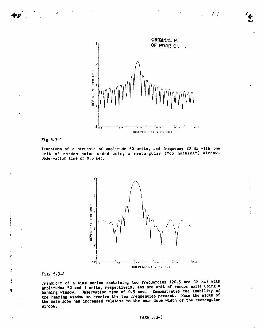
| ItOR,GIN_Lp/_'_ OF.POORr,,
'_oo ' ;oo ' _oo '-- 3_%_ _oo " _oo] NI]EP[NDEN T PlqR] RBL E
Fig 5.3-1
Transform o£ a stnusotd o£ amplitude 50 units, and frequency 20 Hz with oneunit of" random noise added using a rectangular ("do nothing") window.Observation time of 0.5 see.
a
{ i0" 0-_.---_- ...........................IO.O 20.0 aO.O qO.O 50.0
"i INOEPENDf'NT VORi;1(_t f
Fi_. 5.3-2:i
Transform of a time sertea eontatnlns two f_equenoiem (20.5 and 18 Hz) with
q amplitudes 50 and 1 units, respectively, and one unit o£ random noise using aharming window. Obl_.rvatton time o£ 0.5 see. Demonstrates the inability o£the harming window to remolve the two £requen_tem present. Note the width o£the main lobe h&s inQreased relative ¢o the main lobe width o£ the reetengularwindow.
Page 5.3-5
1984026903-099

[
, &OF POOR Q,:,__,,s
1ofk_
b _C_
[IZ> CZ
,m 16 __ 2"0.0 ..... _---• I0.0 )0.0 wO.O 50.0
INDEPENDENTVRRIRB/E
Fig. 5.3-3
Transform of a time series containing two l_equenoles (20.5 and 18 Hz) withamplitudes 50 and 1 units, respectively, and one unit of random noise using aHamming wlndow. Observation time or 0.5 see. Demonstrates the abtllty of the
, Hamming wlndow to resolve the two discrete frequencies.
b
!
tLl| d
2
_' _g__d........ _o.o _o.o 3o.o qa.a I,o.a/ INDEPENDFNT VRRIRBI F
t
Fig. 5.3-_Transform of a tlme series oontalnlng two frequenoles (20.5 and 18 Hz) with
: amplitudes 50 and 1 untts respeottvely and one unit of random noise using aHamming window. Observation time of 0.25 leo. Demonstrates the Inability.even using the Hammingwindow, to resolve the two frequenoles present due toInadequate observation time.
Page 5.3-6
%
1984026903-1 O0
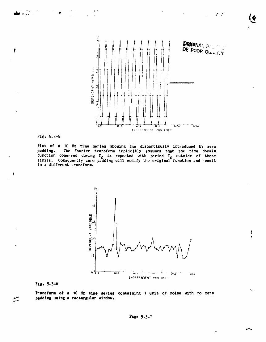
• /
///
o
[i OF.poor
N
/
]NDEPENE]ENT VPlBIFIk[ F
Fig. 5.3-5
Plot of a 10 Hz time series showing the diseontinulty introduced by zeropadding. The Fourier transform llaplieitlyassumes that the time domain
function observed during TO is repeated with period T outside of theselimits. Consquentlyzero padding will modify the orlginalDfunetionand resultin a different transform.
w_dnn
ri-CE>
Z
N
16 0.0 , ..... _ __ _ ,I0.0 _0.0 30,0 _0.0 _0.0
]NPFPFNOENT VRRInPI F
Fig. 5.3-6
Tranlform of a 10 Hz time series oontaining 1 unit of noise with no zerot""', padding using a rectangular window.
Page _. 3-7
1984026903-101
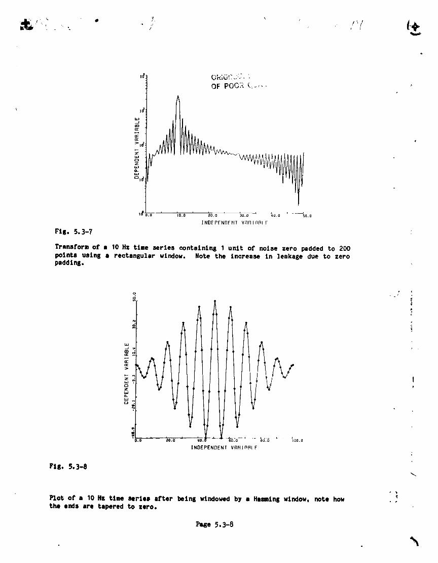
\ t
Iooo.o ,o.o 20.0 30.0 _o.o ...._o.o
INO_PENOFNT VNnIN_F[
FI8. 5.3-7
Transformo£ a 10H= tlme serleseontalnln81 unlto£ nolaezeropaddedto 200pointsusinga rectangularwindow. Note the Increasein leakagedue to zeropaddI nl.
o i
zI#
0=
t , _ _ a ..... _ _ -J0.0 20,0 qO,l_ -- 60.a3 80.0 IQO.O
INDEPENDENT VRRIflBL F
Pig. 5.3.-8
Plot o£ a 10 HI time series i£ter betni windowedby a Hamin8 window, note how ._the ends are tapered to zero.
Page p.3-8
%,
1984026903-102

L/
,o'1
1I
l.l.J_ICD(I
::>
mEItQ
• ,,, 1/ f
_ _,_,
so-u6-..o-.... _5.o _--__T_ " - -;c,_-_..... _.a ..... ?,_.,_]ND_PF_ NJ VqaJnB'F
Fig. 5.3-9
Transform of a 10 Hz time series oontalnln8 1 unit of noise using a Hammingwindow and no zero paddt.g.
I#
L_
rn
CE
. 7
i
i _ _, ,i _ _ L i i i
1 16o.o '1o.o ;too _o,o 400 so.oINDEPENDENTVRRI_BLE
Fig. 5.3-1oTransform of a 10 Hz time series oontalntns 1 unit of noise _slng a Hsmln_window zero padded out to 200 points, note that the leakage level is about theslme as shown In lrllil 5.3"-9.
Page 5 _3-9
1984026903-103

_,,, • ., /"I i:._.p
I
6.0 IDSP OPERATOR DESCRIPTIONS
!
I e
l Usage of AVER Command
The user specifies 'AVER dsname n' where n must be the number of points whleh
he wants averaged into each box. The last box may not be full depending on howtn divides tl_e number of available points. If the user specifies optional ,parameter ZERO, the first box in the average contains only one point. (Thisoption can be used when one wants to avoid having the zero frequency averagedin with anything.) The following ex_,iple utilizes this option, with the rest
.! of the points of dataset SPECTOFF averaged into 8 points per average:
AVER SPECTOFF 8 ZERO
z
I
6.1-1
AVER 4/16/8q
1984026903-104

Usage of CMDHI$ Command
_ This command causes a printout of user responses to the syste_ query "ENTER
COMMAND" that were entered during the current analysis session. It has nooperands. The file that contains these commands is FORO22. DAT and can be
printed after the session ends,
m6.2-1
CMDHIS 4/16/8_
1984026903-105
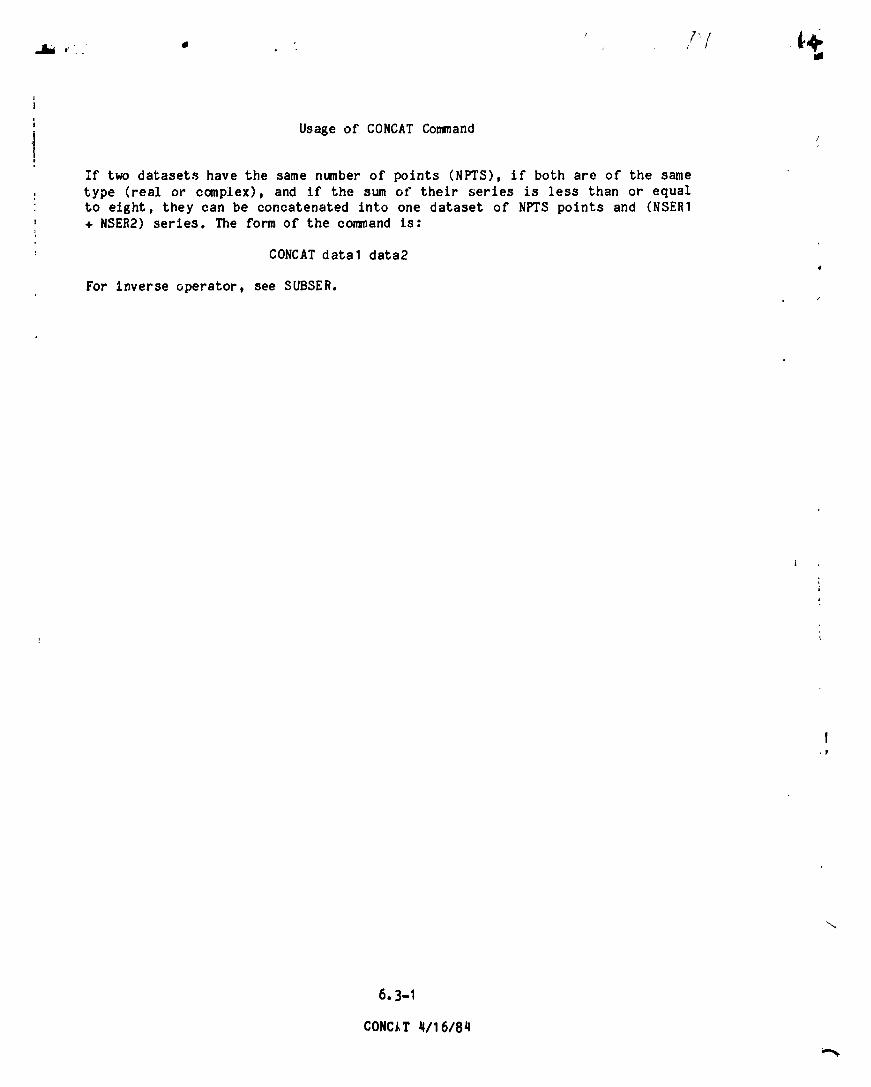
Osage of CONCATCommand
I
If two datasets have the same number of points (NPTS), if both are of the sametype (real or complex), and if the sum of their series is less than or equalto eight, they can be concatenated into one dataset of NPTS points and (NSER1+ NSER2) series. The form of the command is:
CONCATdata1 data2
For inverse operator, see SUBSER.4
i
t
Ip
6.3-1
CONC_TLI/16/84
1984026903-106
Usage of the COPY Command
The IDSP system destroys datasets in Its default working directory[usrld. IDSP] by overwriting the old dataset whet a given operation isrepeated. After any operation, any dataset can be copied into a file of someother name. The first example copies the current ver,_ton of WINDOWinto WIND5in the working directory= the second copies it into a different dtreetory file[usrId.GAMMA]WIND7.DAT.
COPY WINDOW WIND6
" COPY WINDOW [usrid.GAMMA]WIND7
C6.4-1
COPY 4/16/84
J
1984026903-107
I
Usage o£ the DCL Command]|
!
This operator allows the user to temporarily exlt the IDSP process and executeVAX CommandLanguage Commandsvla a subproeess, He w111 recelve the standard"$" prompt. When £tntshed the user should type" "STOP/ID=Oa or "LO" This wlllreturn control to IDSP by terminating the subproeess. NOTE= Typt,_g "'"produoes a message indicating the subproeess was logged o££. It is no _ ,L-£or alarm. The user is now baok in IDSP.
WARNING:Do not do .something £ooltsh in DCL 11ks Control Y, or a deletet _. apurge. When In DCL your LOGIN constraints, such as "deelde" £or delete o,KEEP=2 £or purge are not recognized,
i
!
!l
6.5-1
DCL q/1 6/8q
i
1984026903-108
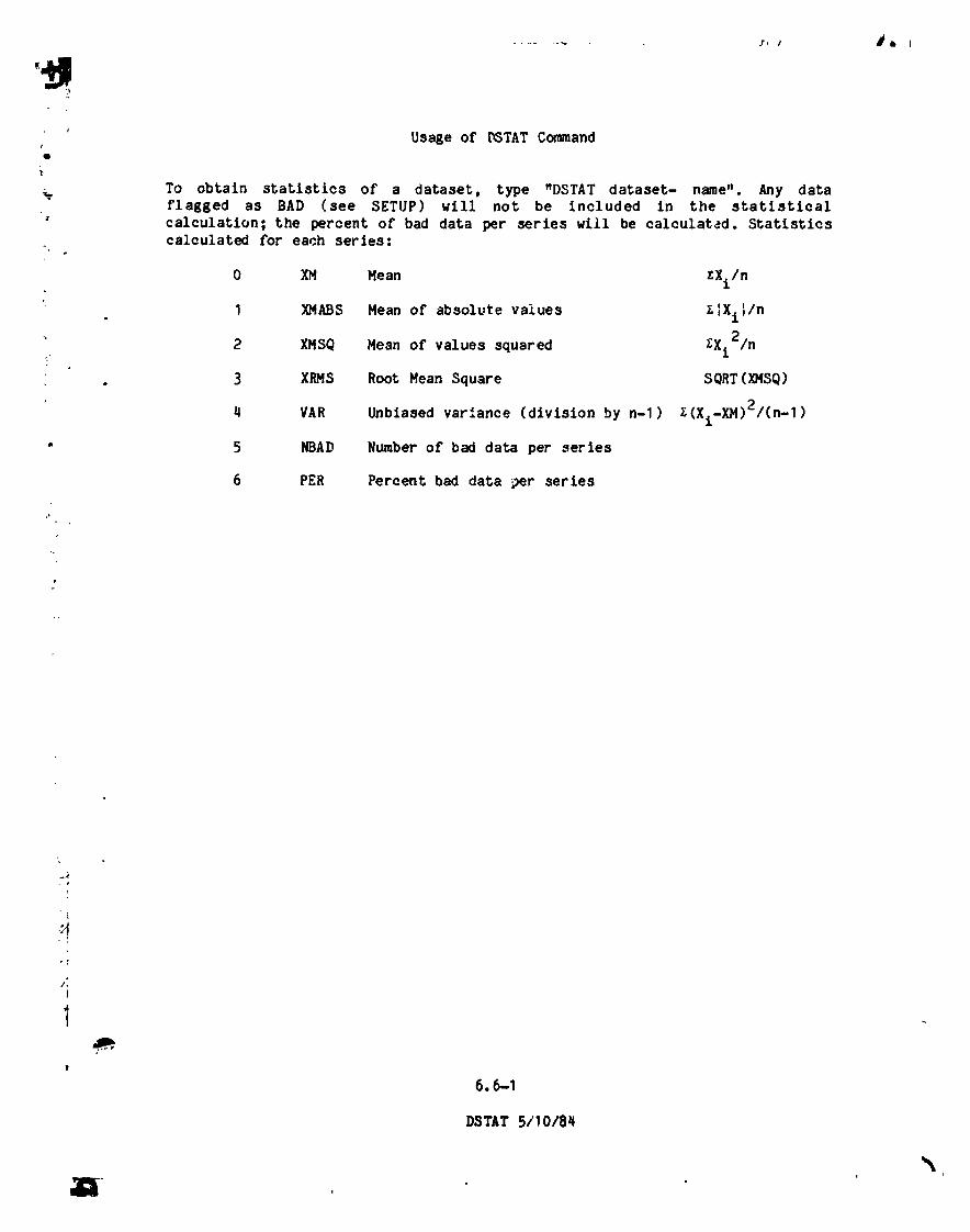
' Usage of ['_TAT CommandrI
To obtain statistics of a dataset, type "DSTAT dataset- name"• Any dataflagged as BAD (see SETUP) will not be included In the statistical
"zcalculation; the percent of bad data per series will be calculatad• Statisticscalculated for each series:
0 XM Mean zXi / n
1 XHAgS Mean of absolute values Z]Xt:/n
XMSQ Mean of values squared _-Xl2/n2
• 3 XRHS Root Mean Square SORT(XHSQ)
q VAR Unbiased variance (division by n-l) Z(Xi-XM)2/(n-1)
" 5 NBAD Number of bad data per series
6 PER Percent bad data ;_erseries
!
/:
I
I
6.6-1
DSTAT 5/10/8q
1984026903-109
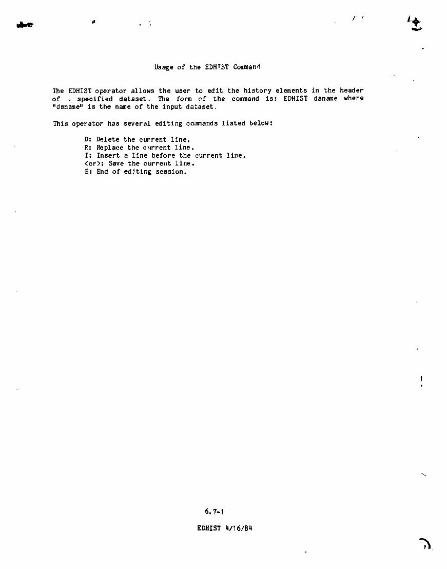
Usage of the EDHT.ST Co.an4
The EDHIST operator allows the user to edit the history elements in the header
of = speeifled dataset, The form of the command is: EDHIST dsname where"dsname" is the name of the input dataset,
This operator has several editing commands listed below:
D: Delete the current line.
R: Replace the current line.I: Insert a line before the current line.<or>: Save the eurretlt line.
E: End of editing session.
6.7-I
EDHIST _116!84
%,
1984026903-110

Usage of EDII ommand
The interactive user at a HP-P_6q8A Graphics Terminal can dynamically flag data
points as BAD (set equal to -99.9) in any real dataset. The EDIT operator
causes a display of up to 500 points to the screen and places the user into
interactive usage of interactive grsphics commands. (To see a list o£ these
commands at this stage, type "HELP".) The only commands that have any effecton the dataset stored by EDIT are those that perform deletions--the EDIToperator will flag them as BAD as soon as the user types "EXIT" to return tothe EDIT operator. If the series had more than 500 points, the next group ofpoints will then be displayed. As soon as editing is finished on one series,EDIT moves to the next one. The form of the command is"
EDIT dataset SER=J ALL
where "SER=J" is optional if the user wants only to edit the jth series. "ALL"
is optional and specifies that if the ith point is deleted in any series, thenit is deleted in all the series.
More extensive documentation on the HP interactive graphics commanos can be
found in Carleton, T. P., LEP VAX User._Guide, NASA TH 84931, October 1982.
6.8-1
EDIT q/16/84
1984026903-111

t
q Usage of the EIG Commandq
: This operator takes as input spectral matrices and does rotation to an:" eigenvalue coordinate system (see Section 5.1 for details). Statistics for
some of the computations are extracted from a dataset created previoosly byoperator DSTAT, operating on a time series data set such as the output ofINTERP or FILTER, i.e., a pre-FFT data set. The form of the command is:
EIG SPECTD SPECTOFF DSTAT MF KCON
1
where "SPECTD" is the dataset containing the diagonal terms of the spectral
:: matrix; "SPECTOFF" contains the corresponding off-diagonal terms; and .DSTAT"
contains the dataset of series statistics. "MF" is optional and is used only
if the user wants the analysis to ass_e that the original series have been
placed into a Mean-Field coordinate system (see operator MNFLD). The diagonals
of the rotated system are stored in EIGD, the off-diagonals are stored in
" EIGOFF, and various scaler parameters are stored In EIGPARM, and the
eigenvectors and eigenvalues associated with the minimum, intermediate andmaximum directions are stored in EIGVEC and EIGVECI.
KCON is an optional parameter of gIG which can be used to select a signconvention for the wave normal vector _ determined in the polarization
analysis (but with arbitrary sign). KCON can have the values I, -I and O,
with KCON = I the default state. In this case, the component kI is forced to
be positive by inversion of _ (multiplying all components by -_) If found tobe negative. For coordinate systems centered at the sun, that will force _ to
have a component outward (along the radius vector direction) from the sun.
• For data coordinate systems defined with X positive toward the sun, the user
, should choose KCON : -I; this forces kI to be in the negative X direction by• inversion of _, again insuring that _ _ave a component outward from the sun. i
If KCON = 0 is chosen, a different convention, based on the direction of
average _, is applied. In this case the quantity BDOTK will be tested; if
BDOTK < o, then _ is inverted and BDOTK recomputed. This forces I_ to have acomponent in the +_ direction.
4Data set EIGPARM contains scaler quantities DEGPOL, (OH, ELIP, THETA, TRTOT,
SNR, BDOTK, and SIGMA. EIG also creates data set EIGVEC which contains inseries I-3, the first three components o£ the eigenvector corresponding to the
direction of minimum variance for that mode. Series 4-6 are the ei_=.nvalues
(minimum, intermediate and maximum, respectively). Also created by operator• EIG is data set EIGVECI which contains the three components of the elgenveotor
corresponding to the intermediate direction of variance (series I-3) and the ,
three eigenvectors corresponding to the maximum direction of variation (series4-6).
WARNING: If the "MF" option has been specified, the normalized magnetic
heliclty (SIGMA) in EIGPARM will not be correct.
For a schematic of operator EIG and its relationships to operators DSTAT and!
lj SPECT and the associated data sets see Fig. 5.1-8.
6.9-1
EIG 4/16/84
,5
1984026903-112
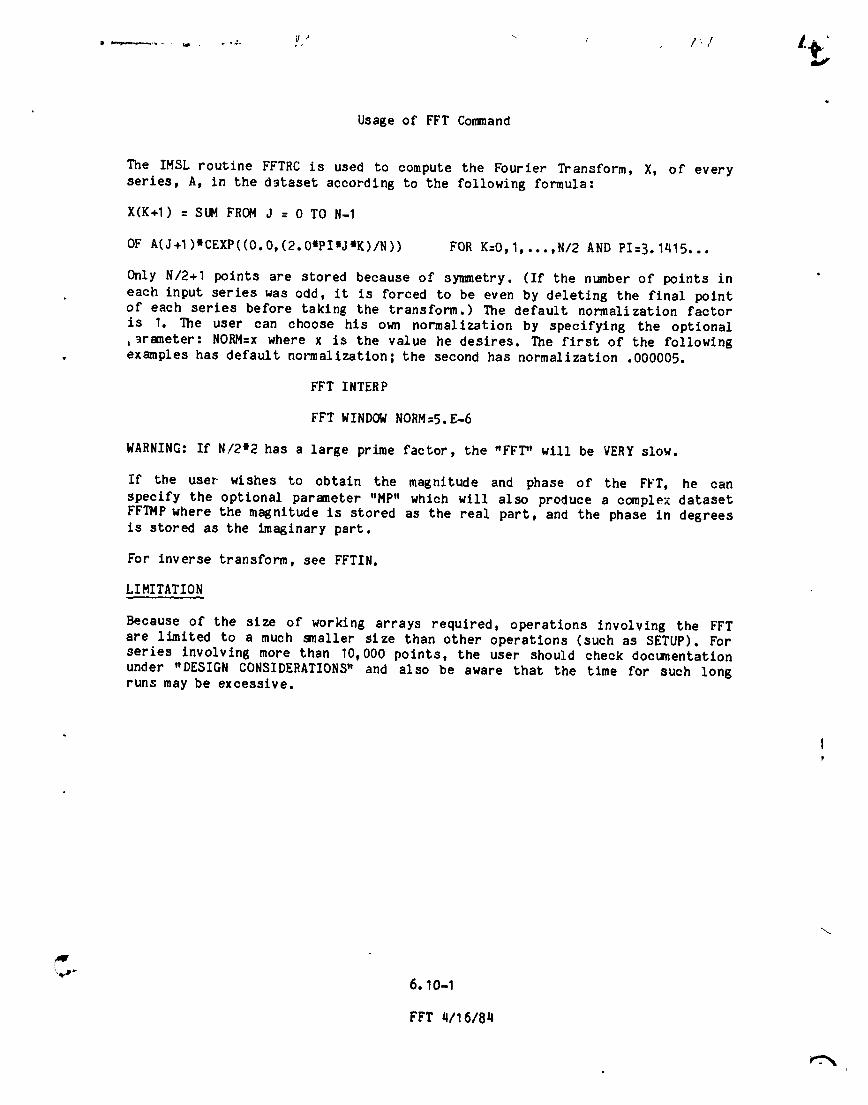
Usage of FFT Command
The IMSL routine FFTRC is used to compute the Fourier Transform, X, of every
series, A, in the dstaset according to the following formula:
X(K+I) = SUM FROM J = 0 TO N-I
OF A(J +I)*CEXP ((0.O,(2.O*PI*J*K )/N)) FOR K=O, I,...,N/2 AND PI=3.1415. ••
Only N/2+1 points are stored because of sy,metry. (If the number of points in
each input series was odd, it is forced to be even by deleting the final pointof each series before taking the transform.) The default normalization factoris I. The user can choose his own normalization by specifying the optional
srameter: NORM=x where x is the value he desires. The first of the following• examples has default no_,alization; the second has normalization .000005.
FFT INTERP
FFT WINDOW NORM=5. E-6
WARNING: If N/2"2 has a large prime factor, the "FF_' will be VERY slow.
If the user wishes to obtain the magnitude and phase of the FFT, he can
specify the optional parameter "MP" which wlll also produce a complex datasetFFTMP where the magnitude is stored as the real part, and the phase in degrees
is stored as the imaginary part.
For inverse transform, see FFTIN.
LIMITATION
Because of the size of working arrays required, operations involving the FFT
are limited to a much smaller slze than other operations (such as SETUP). Forseries involving more than 10,000 points, the user should check documentationunder ,'DESIGN CONSIDERATIONS" and also be aware that the tlme for such long
runs may be excessive.
""'" 6.10-1
FFT 4116184
i
1984026903-113

Usage of FFTIN Commandq
3
"_. The IMSL routine FFTCC is used to compute the inverse Fourier Transform, X, of
every series, A, in the dataset, each containing NPTS. First, a working array
is constructed containing the complete transform, using the conjugate symmetryof the data:
N = (NPTS-I)|2
B(N+2-I) = CONJG(A(I)), FOR I=2,...,N/2
Then X is computed according the the following formula:?
: X(K+I) = SUM FROM J = 0 TO N-1
OF B(J+I)*CEXP((O.O,(-2.0*PI*J*K)/N)) FOR K=O,1,...,N-1 AND PI=3.1415...,a
The default normalization factor is (l/N). The user can choose his own
normalization by specifying the optional parameter: NORM=x where x is thevalue he desires. The first of the following examples has defaultnormalizatzon; the second has normalization .000005.
FFTIN SPECTOFF
. FFTIN SPECTD NORM=5.E-6
For the forward transform, see FFT.
LIMITATION--see FFT
L
/J
r
-i6.11-1
FFTZN q/16/84
1984026903-114
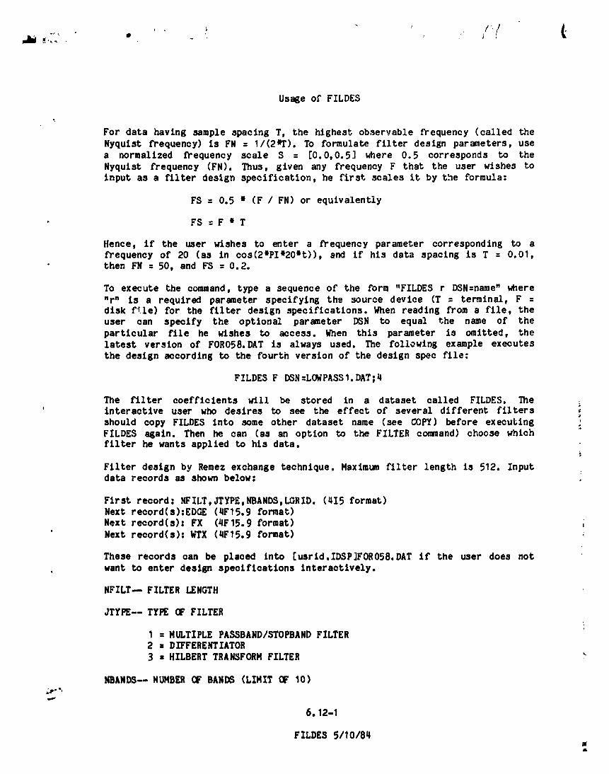
Usage of FILDES
For data having sample spacing T, the highest observable frequency (called theNyqulst frequency) Is FN = I/(2mT). To formulate filter design parameters, usea normalized frequency scale S = [0.0,0.5] where 0.5 corresponds to theNyqulst frequency (FN). Thus, given any frequency F that the user wishes toinput as a filter design specification, he first scales it by the formula:
FS = 0.5 i (F / FN) or equivalently
, FS:FtT
Hence, if the user wishes to enter a frequency parameter corresponding to afrequency of 20 (as in cos(2mPIl2Omt)), and If his data spacing is T = 0.01,then FN = 50, and FS : 0.2.
To execute the command, type a sequence of the form "FILDES r DSN=name" where"r a is a required parameter specifying the source device (T - terminal, F =disk ftle) for the filter design specifications. When reading from a file, theuser can specify the optional parameter D_N to equal the name of theparticular flle he wishes to access. When this parameter is omitted, thelatest version of FORO58.DAT Is always used. The following example executesthe design according to the fourth version of the design spec file:
FILDES F DSN=LOWPASSI.DAT;4
The filter coefficients will be stored In a dataset called FILDES. The' interactive user who desires to see the effect of several different filters ,
should copy FILDES Into some other dataset name (see COPY) before executingFILDES again. Then he can (as an option to the FILTER command) choose whichfilter he wants applied to his data.
Filter design by Remez exchange technique. Maximum filter length is 512. Inputdata records as shown below:
First record : NFILT,_rYPE,NBANDS,LGRID. (415 format)Next record(s):EDGE (qF15.9 format)Next record(s): FX (4F15.9 format)Next record(s): k_X (4F15.9 format)
These records can be placed into [usrld.IDSP]FORO58.DAT If the user does not• want to enter design specifications tnteracttvely.
NFILT-- FILTER LENGTH
JTYPE-- TYPE OF FILTER
1 = MULTIPLE PASSBAND/STOPBANDFILTER2 : DIFFERENTIATOR3 : HTLBERTTRANSFORMFILTER
NBAND$--HUHBER OF BANDS(LIMIT OF 10)_pD -,
6.12-1
FILDES 5/10/8qJA
1984026903-115
LGRID-- GRID DENSITY, WILL BE SET TO 16 UNLESS SPECIFIED OTHERWISE BY A/
POSITIVE CONSTANT.
EDGE(2mNBANDS)-- BANDEDGE ARRAY, LOWER AND UPPER EDGES FOR EACH BAND WITH AMAXIMUM OF 10 BANDS.
FX(NBANDS)-- DESIRED FUNCTION ARRAY (OR DESIRED SLOPE IF A DIFFERENTIATOR) FOREACH BAND.
WTX(NBANDS)-- WEIGHT FUNCTION ARRAY IN EACH BAND. FOR A DIFFERENTIATOR, THEWEIGHT FUNCTION IS INVERSELY PROPORTIONAL TO F.
SAMPLE INPUT DATA SETUP:
32,1,3,00.0,0.1,0.2,0.350.425,0.5 (IN 4F15.9 FORMAT)0.0,1.0,0.010.0, 1.0, 10.0
THIS DATA SPECIFIES A LENGTH 32 BANDPASS FILTER WITH STOPBANDS 0 TO 0.I AND0.425 TO 0.5, AND PASSBAND FROM 0.2 TO 0.35 WITH WEIGHTING OF 10 IN THESTOPBANDS AND I IN THE PASSBAND. THE GRID DENSITY DEFAULTS TO 16.
THE FOLLOWING INPUT DATA SPECIFIES A LENGTH 32 FULLBAND DIFFERENTIATOR WITHSLOPE 1 AND WEIGHTING OF I/F. THE GRID DENSITY WILL BE SET TO 20.
32,2, 1,200,0.51.01.0
If the user wishes to peruse the printout describln8 the filter he can route =the output"to disk via the FLOP command before executln8 the FILDES command.
LIMITATIONS: Avoid desisnin8 a dlfferentiator with an ODD number ofcoefficients. At times the design alsorlthm complains about possibleconversence problems. When deslgnln8 a filter, ALWAYS MAKE A PLOT OF THETRANSFER FUNCTION to ensure that the filter behaves as you desire. Section I5.1.5, and particularly Section 5.2.2, discuss a technique for the systematicdetermination of the stopband ripple and passband ripple using operatorFILOPT. Number of bands is limited to 10 for bandpass/bandstop filter. Themaximum number of coefficients is 512 for any type of filter.
6.12-2
FILDES 51_0/8q
1984026903-116
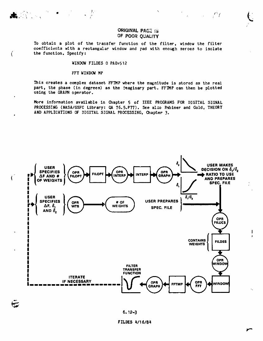
.311'
L.J
/
ORIGINAL PAG_ r,_OF POOR QUALITY
To obtain a plot of the transfer function of the filter, window the filtercoefficients with a rectanaular window and pad with enouah zeroes to isolate
( the function. Specify:
WINDOW FILDES 0 PAD:512
FFT WINDOW MP
This creates a complex dataset FFTMP where the magnitude is stored as the real
part, the phase (in degrees) as the __maEinary part. FFTMP can then be plottedusing the GRAPH operator.
o
More information available in Chapter 5 of IEEE PROGRAMS FOR DIGITAL SIGNAL
PROCESSING (NASA/GSFC Library: QA 76.5.P77). See al_o Rablner and Gold, THEORY
AND APPLICATIONS OF DIGITAL SIGNAL PROCESSING, Chapter 3.
DECISION ON _,/_z• IH ZF-_;&;'; } I _P)'el ,NTERPt'M O_'_HI"e" -"e RATIOTOUSEII ...... AND PREPARES( ,/°'w_'""'sj ,I / .,c.,,_,: '1.1 I, [ USER}_ _ , _,,_. II__,=/SPEOFIESI [ op._ ,_{ #OF '_ USERPREPARES| =1
'-i "
,!!II FILTERII TRANSFERFUNCTION
II IF NECESSARY_ mm IBB BB BIB BIB mm IBB mm BIB BIB BB lib _ BB BII BB BB mlB BBI I _
,,v-
6.12-3
FILDES 4/16/84
r",
1984026903-117
' L£
s
-- Usage of FILOPT%, This operator assists the user in determining the optimum ratio of delta 1 to
delta_ (See Fig. 5.2-1 for definitions of delta1 and delta 2) to use in._. destgfitng a filter with the Remez exchange algorithm.r
To execute the command, type a sequence of the form "FILOPT r DSN=name" where: "_" is a required parameter specifying the source device (T=termtnal, F=dtsk
file) for the filter design specifications. When reading from a file, the usercan specify the optional parameter DSN to equal the name of the particularfile he wishes to access. When this parameter is omitted, the latest version
; of FORO59. DAT Is always used. The following example executes the algorithm: according to the fifth version of the design specification file:
FILOPT F DSN=LOWPASS.DAT;5
: Output is stored in a data set called FILOPT, THis file contains the followingthree series of information."
: 1 -pass band ripple in db- defined as 20mloK(l+deltal)
2 - stop band ripple in db - defined as 20mlog(delta 2)3 - lowest limit of the stop band
The values are calculated nine times per decade for a maximum of five decades.
�Theresolution of the output file is equal to the value of the smallest_ecade. All intermediate points are wrlt+en as fill data (-99.9) to allow for"4
subsequent Interpolation In order to meet the equidistance spacing requirement
of ID6P compatible data sets. _/"_
Each filter Is designed by the Remez exchange techlque. Maximum filter length
is 512. Input data records as shown below:
First record" NFILT, NBANDS, LGRIDNext record(s): EDGE (4F15.9 format)
Next record(s): FX (4f15.9 format)
Last record: IDEC, NDEC
These records can be placed into [usrld.ldsp]FORO59.DAT if the user does not
want to enter design specifications Interactlvely.
° NFILT - filter lengthNBANDS- number of bands
LGRID - grid density, will be set to 16 unless specified otherwise by
V- a positive constant less than 16
• EDGE(2mnbands) - bandedge array, lower and upper edges for each band
/ with a maximum of 10 bands
FX(nbands) - desired function array for each band
i IDEC - starting decade for calculation (power of 10)NDEC - number of decades (maximum of five)
6.13-1
FILOPT 5/10/8qk
1984026903-118
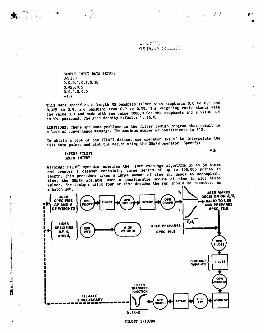
i f
111
SAMPLE INPUT DATA SETUP:32, 3, 0O. 0, O. 1,0.2,0.35
0.425,0.50.0, 1.0,0.0
• -1,4
This data specifies a length 32 bandpass filter with stopbands 0.0 to 0.1 and0. q25 to 0.5, and pasaband from 0.2 to 0.35. The weighting ratio starts withthe value O. 1 and ends with the value 1000.0 for the stopbands and a value 1.0in the passband. The grid density default_ ' _ 16.0.
LIMI_IONS: There are some problema in the filter design program that result ina la_k of convergence message. The maximum number of coefficients is 512.
To obtain a plot of the FILOFI dataset use operator INTERP to interpolate thefill data points and plot the values using the GRAPH operator. Specify:
INTERP FILOPT _"GRAPH INTERP
Warning. FILOPT operator executes the Remez exchange algorithm up to 50 timesand creates a dataset containing three series of up to I00,000 points in
length. This procedure takes a large amount of time and spaoe to accomplish.
Also, the GRAPH operatol uses a considerable amount of tlme to plot thesevalues. For designs u_ing four or flve decades the run should be submitted as
a batohjob. I\
6z USER MAKES.pUSF_._} _ r--'-'l _ I--"-1 _ I_.____OECiSioNON,_,/_,
m_OFWEIO._SI A.OPREPARESI _ _ _, SPEC. FILE,' : l./ ,
' I 1' USERI _ _ ,6,,,, II_._l SPECIFIES I f op. _ . [ # OF _ USER PREPARES I .I
I CON..,./,,,,,,,s,I' &I FIO'E.I TRANSFERI FUNCTION-" ITErlATE I _ _ _ _! ,FNEC'SSARY I\ f _o,._, I.....IJo,.'_J .........J
..................----.__..6.13-2
FILOPT 5/_ 0/8zt
1984026903-119

OF POOR QL',._Li'___
, Usage cf FILTER Command
Subroutine FILTER extracts the filter coefficients from a dataset called
FILDES unless the user specifies that they exist elsewhere by including theoptional parameter "DSN=dataset". The dataset of filter coefficients must be q
created by FILDES before FILTER is executed. Filtering makes contiguous
intervals noncontiguous. To obtain contiguous filtered intervals, use SETUP tocreate one large interval, filter it, and then use the SUBSET operator to
produce the set of contiguous intervals desired. To filter the dataset WINDOWwith the filter coefficients currently stored in FILDES, the user wouldspecify :
• FILTER WINDOW
If he wished to use filter coefficients stored in N91HP04 the user would
specify :
FILTER WINDOW DSN=N91HP04
To avoid accidental aliaslng problems, decimation can be accomplished only as
: an option of the FILTER command. The user should enter "FILTER dataset DEC--n"
where "n" specifies that only the Oth, (n)th, (2n)th,... points will be keptafter filtering. If this option is omitted, every point is kept (no
decimation). WAR;_ING: The decimation rate "n" must be chosen so that I/(2mnUT)
is greater than the lower edge of the lowpass filter stopband where T is the
original sample spacing. Otherwise aliasing will occur. I,
( USER} USeRMA.ES
F---I . o,c,=o,o.eve,.,/ SPECIFIES I ,:,'_'_.,..)m_ FILOPT_m_lN_p_l_ INTERP _(ORAPH )m_- ml_ RATIO TO USE• W'_ AFAND #
Ill [ OF WEIGHTS _;,ILj_ ANDsPEc.PREPARESFILE
II @| SPECIFIES t { OPR _ _/' # OF _ USER PREPARES I ,_' _ _F, 81 / kWT$) " \WEIGHTSJ SPEC, FILE I
CONTAINS FILOES
: WEIGHTS
, &FILTERTRANSFER
FUNCTION _lr
ITERATE I _ _ I---'------! _ • II
6. lq-1
FILTER q/1 6/8q
b,
1984026903-120
_Ii ,' ,._ • "' ' I"1s
J
Usage of FLOP Command
Output for a given operation is routed according to the state of a systemvariable IOUT. The interactive user by default receives output at theterminal. If he wishes to have hard copy of some operation, he simply typesthe command "FLOP". From that point, printout 8oes to [usrid.IDSP]IDSPOUT.DATwhich the user can access accordin8 to his needs after the session ends.
Output to the terminal can agaln be restored by typing "FLOP". Interactiveuser prompts are unaffected by this command.
6.15-1
FLOP q/1 6/8q
1984026903-121
m_
, Usage of GRAFCK Command
/
_- This command allows the user to check on the status of the subprocess that he, initiated via the GRAPH command. The form of the command is:
\ GRAFCK n
where "n" is optional. If "n" is omitted, only one status check is made.• Otherwise, a status check will be make every 15 seconds until either the
subprccess has finished or an" checks have been made. If the subprocess
failed, a listing of the log file will be printed. Note that under some
conditions GRAFCK will claim that the graph terminated normally even when the
subprocess has actually failed. A look at the flle (GRAF.LOG) wlll describeany problems in detail.
6.16-1
GRAFCK 4/16184
1984026903-122
l
,_ Usage of GRAPH Commandg
Plot all the series of any dataset on the VERSATEC plotter in the specified
type plot (0 = linear(x)-linear(y), 1 = ltnear(x)-log(y), 2 =' log(x)-linear(y), 3 = log(x)-log(y)).
Specify line-type desired by (-I = points plotted as symbols only, 0 = pointsi connected by lines only, I = points plotted as symbols connected by llnes).
If only the J-th series is desired, it alone can be plotted by specifying theoptional parameter SF_=J.
Both real and imaginary parts of complex datasets are plotted on separate plot
frames. The user can specify one or the other by the optional parameter "REAL"•_ • or "IMAG,'.
The length of the x-axls can be set by specifying "XLEN=x" where x is in
interval [1,100] (units of inches). The range of values desired in the plotcan be specified via the option SIZE. If this option is chosen, the next
record in the command stream must specify XL, XH,YL, YH In 4GI0.0.
=, To obtain nice labeling in llnear plots, specify limits so that the desired
range is neatly divisible by five. Logarithmic plots are forced to begin and
end on decades. Points that fall outside the plot window are plotted at the
boundary. The independent varlat., is by default plotted as indices where i =O, 1, 2, • • • , NPTS - 1.
If the user wants it in terms of the actual delta spacing of the dataset,these indices will be multiplied by delta if the user specifies option"DELTA".
If plots are specified to be logarithmic in the first variable, the first
point of the plot is automatically omitted.
In the first example, a log-llnear, symbols-only plot is given for everyseries of dataset WINDOW; in the second, only the third series of dataset
INTERP is given a llnear-llnear, symbol-llne plot; in the third, only the real
part of dataset FFT is given a llnear-log, symbol plot wlth actual data
spacing in the independent variable and range limits for X and then for Y:
GRAPH WINDOW 2 -1
m
GRAPH INTERP 0 1 SER=3
GRAPH FFT I -I REAL DELTA SIZE
0., 1.25, 10., 1.E5
b. 17-1
GRAPH q/1 6/8q
1984026903-123

•-'" '" /
J
_4
t If the user wishes to stack several graph co_e=,ands in rapid succession and
then plot them all at once, he should specify the option "HOLD" nn all of them
except the last graph command executed. (WARNING: When this option is used a
dataset name should usually appear only ONCE in the group being held for onegraphing job. Remember that only the last version of the repeated dataset will
_ exist at graphing execution. Depending on the command sequence this final
version may have parameters incompatible with an earlier version, using the
job to fail.)
Special effects can be accomplished by combining other operators with the
GRAPH command. For example, suppose the user wanted a logarit?,_ic plot of onlyI
the negative values of a dataset SPECTOFF. He could enter:
NORM SPECTOFF -I
GRAPH NORM SIZE
where in the size parameter he would specify how closely he wished the plot to
approach zero. The results that are "off seal=" would correspond tonon-negative values in the original dataset.
The actual plotting algorithm accomplishes a VERSATEC plot via a subprocess
which IDSP creates for the user. The first five characters of this process
•; name will be the USRID. To check the status of this subprocess use commandGRAFC K.
A log file of each graphing job is written to GRAFJB.LOG so that the user can
examine it in case his results were different from his expectations. The user
: can easily delete all such files by the DCL command: "DEL GRAFJB.LOG. _'.
If the user has an HP2648A terminal, he can have graphics output sent to the
screen by entering the option "DEV=HP". Up to 500 points of a given series• will be displayed. Then the user can utilize the commands ins!de the
HP-graphics package (for help, type "HELP" after points are displayed). When
he has seen enough of those points, the u_er types "EXIT" to return him to the
next segment of graphic display. He will t.hen see his current graphics display
plus an over-laid alphanumeric display describing the graphics. Graphic
display can be turned on and off via key: "SHIFT GDSP"; alphanumeric via:"SHIFT ADSP".
When the option DEV is used_ the following options are ignored: XLEN, HOLD.
Also even though the lit_-type parameter is required, the present
configuration displays points only. (Inside the HP-package, these csn beconnected by a line by entering "DATA LINE".)
Z
J
6.17-2
GRArH 4/16/84
II.
1984026903-124
Usage of the INTERP Command
'f Interpolation is linear. If any flag values are found, they are replaced byinterpolated values. The example below results in linear Interpolation:
INTERP SETUP
I!
4
6, 18-1
INTERP 4/16/84
1984026903-125
UsaEe o£ HEM command%
f
Z
Maximum Entropy Method o£ computing Power Spectra (Anderson's derivation,
_ Geophysics, Vol 39, Feb., 197q)
This operator handles both real and complex datasets as input. The power
spectrum is output as a real dataset (MEM. DAT). The subroutine COEFFcalculates the filter coefficients A and the subroutine CPSPEC calculates the
power spectrum at frequencies from "_ero to f (Nyquist frequency) with the
desired frequency spacing (FR(_PC). The defan_t normalization factor (NORM)
is I. The default number of filter coefficients (NCOEF) is equal to 2N/In2N
(reference: Berryman, Geophysics Vol q3, Dec. 1978). The default number of
frequency points (NFP) is equal to N/2 + I, where N is the number o£ points in
the original time series.
'he optional parameters may be input as follows:
NORM =X; where X is the desired normalization factor (real)
NCOEF=Y; where Y is the number of filter coefficients (integer). NFD =Z; where Z is the number o£ frequency points (integer)
t
• EXAMPLE:
HEM SETUP
uses defaults values
HEM SETUP NCOEF=50 NFP=75
' NCOEF : 50, NFP = 75, default normalization, NORM = 1
MEM SETUP NORM=5.E-6
uses 8iven normalization factor and gets default values for NCOEF and _P"b
WARNING: The HEM operator is recommended for datasets with less than 1000points, increasing the number of points, NCOEF or NFP will cause HEM to be
L. slower.
LIMITATIONS: Because o£ the size o£ the working arrays required, operations
y_ involving HEM are limited to a much smaller size than some other opera_ors.Therefore, datasets must contain less than 15,000 complex or real
, . points/series for up to 8 series.
/
, f
!" 6.19-1
-1i MEM q/1 6/8q-i
i
1984026903-126
Usage of the M_FLD Command
_,
.p The operator MI_LD performs a transformation from the coordinate systemt of an input vector data set to mean field coordinates. It initially computes
I the _,ean field vector from the input data. In the new coordinate system, ZMFis taken in the direction of the mean fieid. XMF is chosen to lle in one of
_ the orlglnai coordinate planes, determined by the intended use of the
transformed data. The desired plane is selected in response to a prompt: I =- XY, 2 = YZ, 3 : XZ, which appears after the operator is commanded: MNFLD
i SETUP, INTERP, etc. For whatever choice is given for XMF, YMF isM_LD
• properly oriented to complete the right-handed coordinate set. The
transformation is only valid for matrix size = 3.
If spectral analysis is to be performed _t a later stage, note that
transformation to mean field coordinates permits specification of the MF
option on the subsequent call to the operator EIG, for example,
. gIG SPECTD SPFCTOFF DSTAT MF.
This sets a flag MFIELD = I internal to EIG and its supporting subroutines,
and enables application of a special eigenvector coordinate system definitionappropriate for mean field data (see operator EIG documen'.ation).
If the magnitude of the projection of the mean field vector on the plane"_ chosen for the ned X-axls Is less than a specified lower limit (currently
coded into subroutine MFCOMP, which is called by M_LD, as the quantity BLO =
0,01 times the total moan field magnitude), then the rotation matrix for the•: transformation is specified rather than computed (see matrix definitions
"_ following statement numbers 61 and 81 in a listing of subroutine MFCOMP for
ii the cases where XZ and YZ planes are selected, respectively). If the inputdata has a mean vector already In the ZMF direction (with an XY plane
projection less than or equal to BLO), then no transformation is carried out,
and the message "NO ROTATI:J - DATA ALREADY IN MF COORD" appears. A listing• of the mean field vector, and the transformation matrix used wlll appear on
! the terminal screen (or the above "NO ROTATION" message) unless a FLOP is
commanded, which routes the output listings to IDSPOUT. DAT rot later hardcopy
display availability.
!
"l
4
I
6.20-1
M_'LD q/1 6/8q
1984026903-127

!
'4 Osage of NORMCommand
"_ The NORM operator multiplies every point in the dataset by the specifiedfactor. In the following example, dataset FFT is normalized by 0.5E-4.
_' NORM FFT .00005
Li
J!
i
iI!i
III
IP
6.21-1
NORM4116184
1984026903-128

°- ' ,'! |..6.
i Usage o£ the RECPOL Command
_'qt
The operator RECPOL wlll convert from rectangular to polar or polar torectangular coordinates depending on parameter ITYPE.
! If ITYPE=I: rectangular to polar, i£ ITYPE=O" polar to rectangular.
:_!' The data set created as output will be RECPOL.DAT. The location of x,y,z inthe input data set will need to be supplied it converting from rectangular to
"_ polar, while the location of r, theta, phi in the input data set will need to_' be supplied if converting from polar to rectangular. If polar to rectangular
ii the order of output data set will always be IX=x, IY=y, IZ=z. If rectangular
I to polar the order of output data set will always be IX=r, IY=theta, IZ=phl.
EXAMPLE OF INVOKING RECPOL:
, RECPOL datasetn_e
The user will then be prompted to enter whether he/she wants to go from polarto rectangular or rectangular to polar. ( ENTER A 0 IF WANT TO GO POLAR TO
RECTANGULAR, ENTER A I IF WANT TO GO RECTANGULAR TO POLAR. ) on the same llnethe user _iI enter the locations for x,y,z or for r,theta,phl In the input
dataset, as appropriate. The locations will be entered as a number between
[I, #SERIES].
EXAMPLE: O, 1,2, 3 i"' I
in
6.22-1
RECPOL q/1 6t8q
b
1984026903-129
I
II Usage o£ REDO CommandIm
1
' This command allows one to repeat a sequence o£ commands in batch Jobs by
i rewinding the £11e containing the _equence. User specifies 'REDO'.I
-tI
t!
]
s
|
!
I
I
iI
]
I
!
!
6, 23-1
REO0 q/16/84r
1984026903-130

1
i,, Usage of the ROTATE command
The operator rotate performs a coordinate rotation using data sets EIGVEC and
, EIGVECI, which contain the direction cosines ( elgenvectors ) of the variance
ellipsoid computed by operator EIG. i.e., the principal axis of the varianceellipsoid at a particular frequency (NFREO). Thus this operator assumes EIG
' hasalready been executed and the data sets EIGVEC and EIGVECI exist, unless,i the option to enter the direction cosines Interactlvely is selected, In whlch
case the direction cosines are entered from the terminal.
: If EIGVEC and EIGVECI are used for rotation then the first three series of the
EIGVEC dataset at NFREQ supply the direction of minimum variance. The first
three series of the EIGVECI dataset at NFREQ supply the Interme_late direction
and series q-6 of the EIGVECI dataset at NFREO supply the maxlm_ direction ofvariation.
I£ the rotation is to be performed from terminal input, the user wlll be
prompted for the direction cosines. NFREQ is not required and thus the user
wlll not be prompted for NFREQ.
The name of the data set created by this operator is ROTATE. DAT.
!,] TO INVOKE OPERATOR:
ROTATE datasetname
FOR EXAMPLE::1
I ROTATE IS120105 THEN FOLLOW PROMPTS.
THE PROMPTS WILL BE AS FOLLOWS:
i The first Input will be to indicate where in the input dataset to flnd x,y,z
(each should be a number between 1 and the number of series). The next prompt
j will indicate whether the direction cosines will be input from terminal orobtained from datasets EIGVEC and EIGVEC1. If the direction cosines will beobtained from EIGVEC and EIGVEC1 the final prompt will be for the desired
| frequency (NFREO). If the direction cosines wlll be input from the termlnal,there wlll be three prompts to obtain the direction cosines.
EXAMPLE= ( DIRECTION COSINES It_PUTFROM TERMINAL)
1,2, 3 1 . 9890, O. 2,. 1439 • 5567, • 23,. 89 • 1656, -. 2367, • 3q56
, EXAMPLE: ( DIRECTION COSINES FROM EIGVEC AND EIGVECI)
1,2,3 0
6.2q-1
ROTATE 4/1 6/84
t,,
1984026903-131
Usage of SETUP Command
,/
SETUP receives as parameters the endpotnts of the span of time that the userwants analyzed (ITI,IT2), and the interval size (SIZE) he wants processed,specified in units according to IUNIT. (Interval: basle time segment to be
analyzed. Span" Total time composed of contiguous intervals, see Fig. 1.0-3.)ITI and IT2 are converted from date/tlme format into REALm8 variables BEGTIMand ENDTIM in units of seconds.
At the end of the routine BEGTIM is right adjusted by the amount of processing
that has occurred to prepare for a subsequent run. If the left endpolnt is
greater than the right, attempt will be made to input parameters for a new
iI span.I
User data are provided by calls to subroutine INPUT. Data gaps are filled with
flag value BAD (-99.9). Analysis is based on the time sampling rate (DELTIM)I that was found when the buffer was filled with user data.i!
Variables :+.
I IT1(6) = start date/time of span desired [q digit year; day (Jan I = day I);
i! hour; rain; sac; msec].+_ IT2(6) = end date/time of span desired.
+_ IUNIT = parameter indicating units of SIZE: (I = seconds, 2 = minutes, 3 =hours, q = days).
KSER = n--user specification of which series desired from INPUT block-- If n is
positive, choose the first n series in block; if n is negative, choose the
indices represented by each digit, starting at the rlghtmost digit. Forexample, n = 3 chooses series I, 2, 3; n = -351 chooses series I, 5, 3 in that
order. For factors influencing choice of specification order, see SPECT
(operator which calculates spectral matrlces).
SIZE = size of interval to be processed (see IUNIT parameter).
Those records must be placed into FOR051.DAT before processing begins, so that
SETUP can access required parameters'
-_ IT1 (6) format(615)
:' KSER, SIZE, IUNIT format(l I0, F10.3, 110)Y_
IT2 (6) format(615).
] SETUP attempts to collect data for analysis beginning with the time specified
+,+_ as the beginning of the span. The first such point that contalna ell good data
"i defines the start time of the interval being setup, The stop time of the' _pan
(IT2) is an absolute maximum, The endpolnt of the interval is then defined as:
B = MIN(A+SIZEmfunctlon(IUNIT),IT2),
6.25-1
+- SETUP q/1 6/8q.I
1984026903-132

All points found with corresponding times less than B will be included in the,, current interval by SETUP. The point corresponding to B will go into the next
" interval. Any interval may be shortened to insure that good data exists at theendpoint of the interval.
i_ For additional details on asslgr_nentsand files required, see Section q and
'_ Appendix A and Appendix F.
ii Additional span(s) subsequent to the first may be accessed by immedlatelyadding the appropriate three records for each as specified above.
I:I " Ordinarily the user need not concern himself with the size of arrays required.' In response to the command "SETUP", the system sets up the next interval for
processing. If the user also wishes to see a display of the intermediate dataI buffer as It is being filled, he should specify:
SETUP I
If the user has his parameters stored in a file different from FORO51.DAT, he
,,| can access them by specifying the optional paramter "DaN=file", for example:
I SETUP DSN=V2PLASMA.DAT
NOTE: DOnot Control ¥ out of IDSP if processing multiple intervals. This willcause all of the data statements to be relnitlalized and IDSP will start the
!! span at the beginning.
I!il
_ 6
6.25-2
SETUP ¢1/16/8q
1984026903-133

Usage o£ SHOWCommand
Output £or every IDSP operation is placed into a dataset tdentt£ted astoperatton. DATt. History o£ any given dataset can be obtained by typ.ng tSHOWoperatlont; History and data by tSHC_/ operation Dt. Interactive users canobtain hard copy o£ any dataset by routing output to dlsk via the FLOPoommand_ and then executing wSHOWoperation Dt. nD" can be any nonblankcharacter.
6.26-1
SHOWq/16/8q
1984026903-134

' " ;" f'/ It'.";
I't
-\t Usage of SPECT Command
i SPECTuses the output of the Fourier Transform to compute the spectral densitymatrix (PSD). This operator uses as input the first JSER series of therequested dataset where JSER = mln(NSER,q), and NSER Is the number of series
, " in the dataset. All other series are ignored.
Let the ith point of each of the four series used as input to thls operator berepresented by A(I,J), J=1,2,3,4• Then PSD(I,j,k) = XNORM*ConJg(A(I,J))*A(I,k)gives the raw j-kth element of the Ith spectral matrix. For an input dataset
:I containing NPTS and for I = I, 2, NPTS-I XNOPJ4= 2.1((2*NPTS-2)**2),
"I thus folding tilenegative power and adding it to the positive. For I = O,l XNORN= 1./((2tNPTS-2)II2).
The user must specify how many of these matrices he wishes to have addedtogether to make spectral estimates. He is required to specify an odd Integer,
i thus centering the effective frequency of the estimate over the center pointused In estimation. To retain the raw spectral estimates, the user must
i specify or::point per estimate. Each estimate is actually a simple sum._! Suppose the user specified n points per estimate where n=2k+1. The special
! case of zero frequency is accompllsned by retaining the O.-th point withouti modification, and ignoring the next k points.i
If the number of spectral matrices was such that the final estimate is notIt "full", the available points are used and a message is written to the history! of the dataset, detailing how many points were used.
By default, the system dellvers results in unlts/HERTZ by dividing by thefrequency width of the estimate. The O-th estimate is skipped (leftunchanged). If the user wishes his results In terms of power, he shouldspecify the optional parameter POWER.
The following example will form spectral matrices using dataset FFT as inputwlth 7 elements forming each estimate"
SPECT FFT 7
The diagonal terms 11,22,._3,... are stored in SPECTD. The off diagonal termsare stored in SPECTOFFby taking in order the rows of the upper triangularportion of the spectral matrix• The history record details which matrix
iJ element Is assoclated with whlch series in dataset SPECTOFF., In a similar fashion, the coherence and phase arising from the off-diagonali terms are stored as the real and imaginary parts of complex dataset COHPH,i respectively. WARNING: Because of the underlying mathematics, if only one
point is used to form each estimate, the coherence will always be equal to one.
t [ REAL
LIMITATION--see EFT. OATASZTSPECTD
COMPLex CCMPLrX1(.,, OA_AS_T OATAS._T/
FFT SPECrOFFj
6.2T-1
COMPLEX 1SPECT 4/16/8q OATASEt
COHPH l
1984026903-135
!
_i Usage of the STOP Command
i The STOP command is necessary to terminate the analysis session. A cheek will1 be made to insure that any subproeesses initiated for graphing have fin'=shed.
If necessary, IDSP wlll wait until they finish.
6.28-1
STOP q/16/84
d r
1984026903-136
_..".!-,._ , • ' ' I" "
,. /_
','k
¢I
_, Usage of SUBSER Command
.% ,This command allows the user to form a subset of the specified dataset. Theform of the command is:
SUBSER dataset nl n2
where nl is the index of the first series desired, and n2 is the number of
series to be placed into the subset.
:: If the dataset WINDOW has ? series, then the following command will place' series 2, 3, and 4 into dataset SUBSER:
SUBSER WINDOW 2 3
• For an inverse operator, see CONCAT.
/
i
6.29-1
SUBSER 4116184iI
li i
1984026903-137

its, . I
'I
_i Usage of SUBSET Command|
i The user can extract a subset of NP points from a specified dataset beginningt at Index I1 where II Is in the interval [O;NPTS-I] and NPTS is the number of
points in the parent dataset Thls capability allows one to obtain contiguous
! Intervals of data that has been interpolated and filtered.
i contiguous subsets of 500 points each from theThe following example extracts
dataset FILTER which has 1500 points or more. Note that the first argument Isthe index of the starting point, and the second argtment is the number ofpoints to be extracted. In the example we are extracting 500 points e_eh time.
} SETUP!
i INTEPP SETUP
! FILTER INTERP
i SUBSET FILTER 0 500} do chosen ope,'ations on SUBSET(Note thatI1 unless COPY has been used the prev.4.ousSUBSET; has been lost)
r SL_SET FILTE_ 500 500
do chosen operations on SUBSET
SUBSET FILTER 1000 500
If you wlsh to save these subsets, see COPY.
6.30-1
SUBSET q/I 6/8qt=
Pi
1984026903-138

Us_e of TRACE Comm_nd
This command allows the user to form a trace of the specified dataset. Theform of the command is:
TRACE dataset nl n2
where n l is the index of the first series desired, and n2 is the number ofseries to be placeo into the trace. If the dataset WINDOW has 7 series, thenthe following command will sum series 2, 3, and 4 and place the result into
: dataset TRACE:|I
TRACE SPECTD 2 3
Normally operator TRACE is used on data set SPECTD
I
I
i
i iI
.o
6.31-1
TRACE 4/1 6/84
i
1984026903-139
Usage of WINDOW Command
WINDOW windows every series In the dataset according to user specifications.(0 = Rectangular, i = 135 cosine taper, 2 =Hanning, 3 = Han_ing.)
The dataset can be padded with zeroes out to point number "n" (after'windowing) by specifying the optional parameter "PAD-n". For example, aHanning window of dataset IN'£ERP is accomplished by:
WINDOW INTERP 2
A rectangular window of dataset FILDES, then padded w_th zeroes out to point20q8 is accomplished by:
WINDOW FILDES 0 PAD=2Oq8
E. 32-i
WINDOW5110/84
1984026903-140

Usage of WTS
LOW P_SS FILTER WEIGHTS ESTIMATION O_ERATOR
WTS Calculates an estimate for the number of filter weights necessary todesign a given filter using the Remez exchange algorithm. To execute, inputthe start and stop frequencies of the transition band, sampling frequency ofthe data, and the desired pass band ripple and stop band ripple.
SAMPLE INPUTS:" First record: Fi,F2,FS
Second record: PBR,SBR
FI - Start frequency of the transition bandF2 - Stop frequency o£ the transition bandFS - Sampling frequency of the data
PBR - Pass band ripple (20mlog(1+deltal))
SBR Stop band ripple (20%og(delta2))
Two types of ouput can be generated by WTS. First is a printout that can besent to the terminal screen or to a flle named [usrld.ldsp]Idapout.dat. Tosent the output to a flle the user must execute the command FLOP just beforethe execution of this operator. Thls output contains the input parameters,
the normalized band edges, delta., delta^, the ratio between deltal anddelta2, and the number of filter wel_hts calc_ulated.
( SAMPLEOUTPUT:TRANSITION BANDFREQUENCIES= 0.6 - 0.8SAMPLINGFREQUENCY= q,q
PASSRIPPLE = 1.0 DBSTOP RIPPLE = 50,0 DB
BANDEDGES= 0.0000 0.136q 0.1818 0.5000
DELTA1 = 0,12202, DZLTA_ = O. 00316
DELTAIlDELTA2 = 38.5855q
NUMBER OF FILTER WEIGHTS = 32.q59
The second output contains the necessary input parameters for the FILDEScommand. These values will be stored in the current version of FORO58.DAT.
SAMPLE OUTPUT:33, 1,2,00.0,0. 1361,0. 1818,0_51.0,0.01. O, 38. 586
LIHITION: WTS wlll produce a FILDES input datsset with an odd number of f_Iter_-,' weights (maximum of 511 weights).
6.33-1
WTS 5/10/8q
1984026903-141

£;
BIBLIOGRAPHY
1) Anderson, N., _ortnotes: On the calculation of filter coefficients for
: maximum entropy spectral analysis, Geophysics, Vol. 39, No. I (February,197q), pp. 69-72.
2) Bergland, G. D., A Guided Tour of the Fast Fourier Transform, IEEESpectrum, July 196_.
S) Berr_an, J. G., Choice of operator length for maximum entropy spectralanalysis, -Geophysics, Vol. q_3, No. 7 (December 1978), pp. 138q-1391.
q) Brigham, E. 0., The Fast Fourier Transform, Prentice-Mall, 1no, EnglewoodCliffs, New Jersey; 197q.
5) Burg, J. P., Maximumentropy spectral analysts, presented at the 37thAnnual International SEG Meeting, Oklahoma City, OK, October 31, 1967.
6) Carleton, T. P., LEP FAX Users Guide, NASUGSFC TH 8q931, October 1982.7) Espenak, F., K. W; 'Behannon, _. H. Mlsh, J. it. Jones, LEP Generalized
5_ctral itnalysts System, NItSA/GSFCX-69q-77-250, Revised April 1979.8) Fowler, R. it., B. J. Kottck and R. D. Elliot, Polarization Analysis of
Natural and Artificially Induced Geomagnetic Mtcropulsattons, J.-Geophys. Res., 72, 2871, 1967.
9) Hamming R. W., Digital Filters, Prentice Hall, Inc. Englewood Cliff, NJ07632, 1977.
10) Harris F. J., On the Use of Windows for Harmonic Analysis with theDtsoret e Fourier TransC.orm_ Proceeding Of the IEEE, Vol 66 No 1, Jan.1978.
11) IMSL Library, Reference Manual, Edition 9, IMSL, Sixth Floor GNB Bldg,7500 Bellatre _Ulevard, Houston Tx 77036, 1982
12) Jenkins, G. M. and D. G. Watts, Spectral Analysis and its Applications,Halden-Dey, San Francisco, 1968.
('_ 13) Lanczos, C., itpplied Analysis, Prentice-Hall, Englewood Cliffs, HJ, 1956.14) Lanczos, C., Vlscourse on Fourier Series, Hafner Publishing Co, New York,
1966.15) Metthaeus, W. H., M. L. Goldstetn, Stationarity o! Hagnetohydrodynemlc
Fluctuations in the Solar Wind, J. Geoph_.s. Res. 87, NO. A12,103qT,December 1, 1982.
16) Metthaeus, W. M., M. L. Goldstein, Measurements of the rugged tnvartantsof magnetohydrodynamic turbulence in the solar wind, J. Ge0phys. Res.87, 6Oll, 1982.
17) Me_haeus, W. H., M. L. Goldstein, and C. Smith, Evaluation of magnetichelicity in homogeneous turbulence, Phys. Rev. Lett, q8, 1256, 1982.
• 18) Means, J. D.. Use of Three-Dimensional Covariance Matrix in Analyzing the IPolarization Properties of Plane Waves, J. Geopi;ys. Res., 77, 5551, 1972.
19) Mtsh, W. H., Editor, CommonlyUsed Digital Tape, Disk and Card Formats,NASIt/GSFC, X-69q-76-2q2; Revised Feb. 1981.
20) Moffatt, ft. K., Magnetic Field Generation in Electrically ConductingFluids, Cambridge _t'verstty Pr'ess, MY, 1978.
21) Otnes, R. K. and L. Enochson, Digital Time Series Ana!_sts , J. Wiley _ndSons, New York, 1972.
22) Programs for Digital Signal Processing, IEEE Press, 1979.23) Rablner, L, R.; B. GOld, l_eory and Application of Digital Signal
_, Prentice-Hall Inc., Engleuood Cliffs, N J, 1975.24) Rankih_ ._nd R. Kurtz, Statistical Study of Mioropulsation Polarization,
J. Geophys. Res., 7_55, 54q_, 1970. \25) 3chaff, W. "E.. Course Notes: Modern Methods of Dt6ital Signal Processing,
• Integrated Computer 'Syst'ems, Iilo,- -Ootob;r 1979._"_ 26) Sentman, D. D., Basic Elements of Power S corral Anal sis, U of Iowa
Preprint 74-5, 2_2, January197q.
BIBLIOGRAPHY
i"
1984026903-142

._,. j • ' , f"/
_4
ACKNOWLEDGEMENTS
!The authors would llke to acknowledge and thank M. Goldsteln end W. Mattheeus
__ for aiding in the initial debugging of the syst_, for their theoreticalcontributions, operator development, helpful suggestions, and careful reviewor" the manuscript. We thank F. Ottens for his contributions to operator
:i develoi_ent, maintenance, and the Appendices.
i
,!
lt
I
Ii
i
i
I
i Pl
ACKHOWI£DGEMENTS
1984026903-143
............ 7 ' ¢', l #_,,"1
APPENDIX A Writing INPUT Routines
The user interfaces his particular data to the IDSP system via an input
routine which delivers a block of data to the system whenever it is needed.
The routine must be specified as SUBROUTINE INPUT with argument list:
(BLOCK,TIME,MAXBLK,MEMBER,NSER,DELTIM,PCNT,BAD,EOF).
The routine arguments which subroutine INPUT muse supply are as follows:
BLOCK : two-dimensional real*4 array containing up to 256 points in each of up
- to 8 series. This array must have dimension (256,8).
TIME = REAL*8 array containing the time associated with each point, specified
in seconds since the beginning of 1960. This array muse have dimension (256).To convert calandar (Jan I = day I) date-time format into seconds since 1960,
a special sutroutine has been supplied. Fill real*8 variable XTIME with theconverted time by coding:
CALL DATTIM (XTIME,YEAR,DAY,HOUR,MIN,SEC,MSEC)
where all variables except XTIME are integer*2. YEAR is specified as a
four-dlgit integer. To convert decimal days (Jan I = day O) to seconds, use asupplied subroutine:
CALL DECTIM (XTIME,YEAR,DDAY)
where real*8 XTIME is returned from inputs integer*2 YEAR (4 digits) and
real*8 DDAY(Decimal Day.Fraction of Day).
MEMBER(INTEGER*4) = number of points INPUT is delivering on this particularcall
NSER(INTEGER*4) = number of series being delivered to the system (max = 8)
DELTIM(REAL*4) = time interval in seconds between adjacent points
PCNT(REAL*4) = percent variation user is willing to allow in DELTIM (enter I_as ,01)
' IEOF = logical variable which the INPUT routine must set to .TRUE. whenever anend of file occurs during read, or when the user desires to inform IDSP not to
continue calling the INPUT routine.
The following are system arguments and must not be altered:
MAXBLK(INTEGER*4) = maximum number of points allowed in each series = 256
BAD(REAL*4) = IDSP flag for bad data. Any bad data detected by the input
routine should be set to BAD (e. g. BLOCK(25,2) = BAD). Missing data shouldalso be set to BAD.
\
In addition, the first call to INPUT should cause character variable HISTIN to
be initialized to a string of up to 80 characters describing the input
Page A-1
APPENDIX A 11/10/82
1984026903-144

#
!
VI dataset. This variable must be CHARACTERW80and be specified: ,,,
COMMON IHISTI/ HISTIN
.!For examples showing dimensions and variable declarations, see
SYS$IDSP:INPUT.FOR, INPUTVOY.FOR, which appear in this APPENDIX."'t
If the user desires to test simulated data, an easy interface is accomplished
by writing an input routine similar to INPUTGEN.FOR, located in DRC3:[IDSP],replacing the statements that do the actual data generation. The user could
•; make a copy of thls routine and modify it to sult his needs. /
c Subroutine INPUT (stored in INPUT.FOR)l,
c IDSP
: C R.M. Wenger (CSC) 3/27/81, C
,; c reads data created by GENDAT.FOR; c Used for testing purposes.
cmmmmmmmmmmmmmaammmmmmmmmmmmmmmmmmmmmmmmmmmmmmmmmmmmmmmmummmmmmmmmmmmmmm
' C
SUBROUTTNE INPUT(BLOCK,TIME,MAXBLK,MEMBER,NSER,DELTIM,PCNT,BAD,l 1 EOF)
I COMMON /HISTI/ HISTIN
1 CHARACTERm80 HISTIN
4
REALm4 BLOCK(256,8)4 REALm8 TIME(256),START
LOGICAL INIT,EOFDATA INIT/ .FALSE./
IF(INIT) GO TO 75
OPEN(UNIT=II,TYPE='OLD',NAME='[ZBRMW.IDSP]FOROII.DAT', i
1 _ORM='UNFORMATTED', READONLY) IREAD(11)HISTINRZAD(11) DELTIM
INI? = .TRUE.EOF = .FALSE.
PCNT : .005 i"PI = 3.1415926NSER = 5
C75 CONTINUE
} MEMBER = 0
i DO 100 I=1,8READ(11,END=990)(BLOCK(I,J),J=1,NSER),TIME(I)
i MEMBER = MEMBER + 1100 CONTINUE
RETURN990 EOF = .TRUE.
RETURNEND
!
Page A-2
APPENDIX A 11/10/82
%
I
1984026903-145

¢
c
c Subroutine INPUTVI (stored in INPUTVOY.FOR)c IDSPc
c R.M. Wenger (CSC) 11/12/80.c
i.
c INPUTV provides input from Voyagerl summary data.c structure:
!c set PCNT according to spacecraft timing variations
! c set MEMBER = 0r c on first execution, decide which data by _ecord of FORO52.DAT
c loop 1:c If member + number of type .gt. MAXBLK goto Done:
_! c read record
' c if EOF, skip 'extract' set EOF to true.returni - c set basin tlme of block in decimal day units
._ c depending on type of average desired,c call 'extract' as a function of the desired arrayC increment MEMBER
c go to loop I:
SUBROUTINE INPUT(BLOCK,TIMBLK,MAXBLK,MEMBER,NSERI,DELTIM,PCNT,BAD,I EOF)COMMON /HISTI/ HISTINCHARACTER*80 HISTINREALm4 BLOCK(256,8)REALm8 TIMBLK(256)INTEGERm4 HEM(3)LOGICAL EOF,INITDATA INIT /.FALSE./DATA HEM/ I, 5, 25/
i CINCLUDE 'U2LJMVOY.FOR/LIST'
CIF(INIT) GO TO 100OPEN(UNIT=II,TYPE='OLD',READONLY,I ACCESS='SEQUENTIAL',RECORDTYPE='VARIABLE',2 FORM='UNFORMATTED',BLOCKSIZE=892,RECORDSIZE=q96)
• READ(52,12) HISTINREAD(52,11) IAVPCNT = .005
EOF = .FALSE.i INIT = .TRUE.
I 100 CONTINUE4 ci MEMBER= 0• 200 CONTINUE
'i IF(HEMBER + ME_4(IAV) .GT. MAXBLK)RETURN
READ(11,END=600,ERR=650)(RqD(I),I=1,q96)IF(IAV .EO. I) CALL EXTR(Mq8,BLOCK,TIHBLK,IDETE,NSERI,MEM(IAV),
1 IAV,DELTIM,MEMBER,BAD)IF(IAV ,EQ, 2) CALL EXTR(M96,BLOCK,TIMBLK,IDATE,NSERI,MEM(IAV),1 IAV,DEL£IM,MEMBER,BAD)
Pose A-3
APPENDIXA 11/10/82
1984026903-146
i
IF(IAV .EQ. 3) CALL EXTR(HI92,BLOCK,TIHBLK,IDATE,NSERI,MEH(IAV),Q,
I IAV,DELTIH,HEHBER,BAD)MEMBER = HEHBER + HEH(IAV)
"_ GO TO 200
600 EOF = .TRUE.RETURN
_ 650 WRITE(6,61)IERR = 3STOP,
!I FORHAT(I5)11
12 FORMAT(A)
61FORHAT(IX,°mmmINOTICE: ERROR READING INPUT FILES. SESSION STOPS lw)
-.-i END
e'
Pase A-4
APPENDIX A 11/10/82
I,
1984026903-147

C ¸
c Subroutine EXTRc
c EXTR gets data specified in array POINTS, and places it into
c BLOCK; it places associated times into TIMBLK. NPOINT is number
c of points in passed array POINTS.c inside extract:
c convert flag data to BAD
c place data into BLOCKc calculate times (as let of type) and place into TIMBLK
c deliver DELTIM (in seconds)o
c
SUBROUTINE EXTR(POINTS,BLOCK,TIMBLK,IDATE,NSERI,NPOINT,
I IAV,DELTiM,MEMBER,BAD)" REAL*4 POINTS(275),BLOCK(256,8),DT(3)
REAL*8 TIMBLK(256),TIME
INTEGER*2 IDATE(6),IYRDATA FLAG/999./
DATA DT/ 48., 9.6, 1.92/NSERI : 7DELTIM = DT(IAV)
C
IYR = IDATE(1) + 1900
CALL DATTIM(TIME,IY _ TE(2),IDATE(3),IDATE(4),IDATE(5)
I ,IDATE(6))TIME = TIME - DELTIM
- DO 200 I=I,NPOINT{ TIME : TIME + DEI.TIM%r
TIMBLK(MEMBER+I) : TIMENGET : I !
DC !_0 J:I,NSERIBLOCK(MEMBER+I,J) = POINTS(NGET)
IF(POINTS(NGET) .EQ. FLAG) BLOCK(MEMBER+I,J) : BADNG_I = NOET + NPOINT
150 CONTINUE200 CONTINUE
RETURNEND
Page A-5
aPPENDIX A 11/10/82
1984026903-148

APPENDIX B-WRITING USER DEFINED OPERATORS
The user can write operators of his own and interface them into the system.
For how to write them, see below. Object versions of user operators can be
interfaced into the IDSP system via the link step (see How to START Using IDSP
Section 4.0). The sequence has been designed so that the users library is
searched ahead of the IDSP system.
The user can write his own operators and interface them into the IDSP system
by adhering to the following conventions:
• 1. The name of the subroutine must be "Ui" where i=0,I,2,...,19.
2. Returns must always be "RETURN I"
3. Use an INCLUDE statement to get current system initialization. Usage of the
INCLUDE statement helps insure compatibility with IDSP system updates. Failureto use INCLUDE may result in subroutine incompatibility as IDSP is updated.
4. CMD is a character striog containing user parameters specified at execution
according to the desire of this operator. See "OPERATOR PARAMETEPS VIACHARACTER STRING" in APPENDIX C.
5. HISTO Is an array of character _trings in which the user describes in words
tileeffect of this operation on the data.
6. HIST is the system history of operations that is retrieved with the givendataset when it is fetched. That history is actually a composite of all
HISTO's that have detailed the meaning of each operation affecting the given
dat_set. Any new operation history in HISTO is appended to HIST by call tosubroutine HISTUP. This subroutine takes NHISTO elements of array HISTO,
appends them to the NHIST elements of array HIST and updates NHIST = NHIST +NHISTO. It also includes a safety check to prevent NHIST from getting too
large.
7. IDGET, IDSAV are variables containing th_ names of the datasets
respectively that the user wishes to fetch, and then save after appropriate
operations.
, 8. Details on data structures involving subroutines FETCH and SAVE can befound in APPENDI' C.
P
9. For maximum utility in interactive mode, all printout except prompts shouldbe written to logical unlt number IOUT. This variable must not be altered by
the subroutine. All user prompts should be written to logical unit FORO06.
10. DEG, PI, BAD are system parameters and must not be altered and arerespectively: 180/3.141593, 3.141593, -99,9 (BAD is flag for bad data).
11. IDSP1 contains the space available to the user for working arrays, LIHSPCand MAXSER are system parameters (500,000 and 8 respectively) and must no_ _ealtered,
\
• 12. The dimensions needed for arrays are calculated by subroutine LIMSET and
Page B-1
APPENDIX B 11/10/82
1984026903-149
are stored in array LIM. This subroutine must be called so that .rays can beproperly dimensioned. For description of parameters, see LIMSET.FOR, APPENDIXC.
The operator NORMls an example requiring one input dataset (see NORM.FOR);The operator EIG is an example requiring more than one input dataset (seeEIG.FOR).
LIST OF LOGICAL NAME ASSIG_'_S
SYS$IDSP:IDSP = DRC3:[IDSP]IDSP/
!II.I
J
Pase B--2
APPENDIX B 11/10182
1984026903-150
_PP_NDIX C-DESIGN CONSIDERATIONS FOR IDSP
, USER DATA STRUCTURE AND MANIPULATION
1. Assume input data from spacecraft is real; usage of complex valuesoccurring only after Fouri_ Transform.
2. Use a single set of input/output routines to store or retrieve either real
or complex values, with array passed as a single parameter.
' 3. Each operator saves output into dataset called 'oper'.DAT.
4. Dataset names have arbitrary length up to maximum total of thirtycharacters.
5. User data is stored in a two-dimensional array where the first dimension
refers to the number of points per series to facillltate operations with eachseries as a unit.
6. Output from each operator is written unformatted to dlsk as data(npts,nsel)
regardless of whether the data are real or complex.
7. Each operator module can set up varlable domain array sizes according to
the needs of the dataset being accessed and the working array requirements of
the operation. _1_eparameters NSER and NPTS are extracted from the dataset and
used by the subroutine LIMSET to set up an array LIM defining the dimensions.
The space available for these large arrays is found in IDSPI/SPACE. Eachmodule splits this up as needed. Then these arrays and dimensions are passed
to a routine that does the actual operation. Because of extra space
requlrememts, FFT operations use a different routine LIMFFT to apportion spaceneeded. For how these requirements are calculated, and limits involved, _ee a
listing of the subroutine.
8. To fapilitate implementation, each operator uses an "INCLUDE" statment:
"INCLUDE 'OPER.FOR'" and each subprocessor uses "INCLUDE 'OPERI.FOR'". Each
routine can add any other statments that are specific to its needs.
9. Each operator module can specify what format it desires to have complex
arrays in memory. If JTYPE : 1, DATA is real and must be dimensioned REAL iDATA(LIM(1),LIM(2)); parameter JFORM is ignored. If JTYPE = 2, DATA is
complex, and will be retrieved according to parameter JFORM. In the call toSUBROUTINE FETCH, if the JFORM parameter = I, data will be returned to array
DATA as a complex variable; DATA must be specified COMPLEX
DATA(LIM(1),LIM(2)). If JFORM = 2, data will be returned to array DATA as two
real arrays, with tt_e real part of each series stored in DATA(npts,J) and theimaginary part stored in DATA(npts,nser )Ô�„�whereDATA must be spectfled REAL
DATA(LIM(1),LIM(2)). Similarly, data ar_ accessed by SUBROUTINE SAVE according
to identification of data type and storage format glve_ by parameters JTYPE
and JFORM. When the calling routine is dimensioned in this fashion, _he
input/output subroutines will correctly save or fetch any of the three type_
of formats, retaining the flexibility of passing a single data array through \an argument list. NEVER allow dimensions and NPTS and NSER to take dual roles.
_...: Such a structure encourages VERY SUBTLE ERRORS.
Page C-1
APPENDIX C 11/10/82
-
1984026903-151
10. Due to special working arrays needed for operators FFT, FFTIN, and SPECT,
._ a special subroutine (LIMFFT) was written to define locations and lengths ofnecessary arrays to make all these operators compatible. For any Oataset to be
% input to any one of these three o_rators, it mu_t be of size compatible with
_ all three operators,
11, All input/output of user datasets is centre]led by calls to subroutines
whose listlng can be found in SYS$IDSP:IO,FOR. Further details on subroutine
parameters are found in the comments of this li&tlng,
12, With each dataset are stored arrays .PARM and IPARM as follows: XPARM(1) =current data spacing XPARM(2-3) : time in seco_ids associated with first point
(REALI8). XPARM(q-5) = time in seconds associated with last point (REAL_8).IPARM(1) = pointer indicating current domain of dataset (I : time (seconds); 2
: frequency (Hertz)). IPARM(2) : version number of system (see FIXVER inIO.FOR).
,. MISCELLANEOUS DETAILS Logical File Names:
The following FORTRAN logical unit numbers are used by IDSP and its assvciat_droutines.
' I) User input parameters: 51-79
LOGICAL UNIT #S USE
, 51-79 input to user INPUT routines
51 input to SETUP routine... 58 input to FILDES (design filter)
57 character strings specifying operationsD
• 2) User data: 10-19
LOGICAL UNIT #S USE
11 experimenter data test routine read byDRC3:[IDSP]INPUT.FOR
13 INPUT/OUTPUT parameters i17 81ve interactive user hardcopF
3) System Character strings: 20-29
LOGICAL UNIT #S USE
21 HELP files
,_ 22 command history
23 submit plots
24 parameters needed for separate plot
:, Jobs25 cluster names for plot; also used to
•. associate Command Event Flag Clu_ter
/ with a process"I
_ 4) Error Conditions: 90-99J
LOGICAL UNIT #S USE91 error condition in Versaplot batch job
Fage C-2
APPENDIX C 11/10{82
1984026903-152
" I, I t._.r
Event Flags
Event flag_ 64 and 65 are reserved for testing the 3tatus of graphing jobs.
_vent flag I is used in GRAFCK. See operators GRAFCK, GRAPH. See programsGRAFGOOD, GRAFGOOF, and GRAFJB.
IDEAS
I. Edit wild points using IMSL routine ICSMOU
OPERATOR PARAMETERS VIA CHARACTER STRING
i
During execution, parameters for a given operation are transmitted to the
, system via a set of substrings in the character variable CMD. The command, string for any given operator is:
command pl p2 P3 ....
where "command" is the name of the operaticn desired, and the "pi" are
parameters used by the operator. The different substr!ngs in the variable CMD
are always separated by blanks. Each operator is of the form "Subroutine
opera(*,CMD)". By the time execution is inside this subroutine, the "command "has been stripped off and CMD ts left as:
pl p2 P3 • • •
Access to these parameters is facilitated by calling one of two subroutines:
CALL STRING(CMD,STRI) or CALL STRNUM(CMD,NUM). Both return the value of the
leftmost parameter to the second argument, and return CMD with the first
parameter and first blank stripped off, i. e.,
p2 P3 • • •
Us_ STRING when you wish to interpret the parameter as characters; use STRNUMwhen you wish to interpret it as an integer. Usually "p1" is the name of the
• dataset desired as input for the operation. Hence, many operators CALL I
ASK(CMD,IDGET). This routine calls STRING to obtain the dataset name• If CMD
was blank (interactive user forgot to enter dataset name before carriage
return), the user is prompted to enter the dataset name. If the user enters an
invalid value for an optional parameter, the system will do one of two things:
I) issue prcmpt for new entry, 2) ignore the entry and use the default.
Page C-3
APPENDIX C 11/10/82
1984026903-153
!
APPENDIX D-Execution of Batch Jobs
Batch jobs require everything that interactive jobs require plus a commandflle called IDSPBAT.COM which contains the commands desired. This file must
exist in the same directory that contains the other user parameter files.
I) Create, for example, the following file called IIX3PBAT.COM
$ CREATE FOR 057.DATSETUPINTER P SETUP
• SHOW INTERP DFFT INTERP
SHOW FFT D
STOP
. $ EXIT
2) On the terminal execute the command file IDSPBAT.COH
as follows •
@IDSPBAT. COM
This will create the file FOROS?.DAT which will be read by the batch job.
3) Create a command file_ for example BATCH.COMt conta!ning the following:
SASSIGN your data FOR 011
any other assign statements your job may require$@SYS$IDSP:IDSP linknames or NOLINK
4) Submi; the command file, for example BATCH.COM
I
I
l
!
l.w _
Page D-1
APPENDIX D 315184
1984026903-154
iAPPENDIX E-Conventions on DATASET NAMES
¢
_ When a dataset must be specified within a command, it can be entered in simple
, form, or can be fully quaJified. Unless explicitly specified otherwise, datatype ".DAT" is assumed. Simple form defaults to directory [usrid. IDSP]; for
,, example dataset:INTERP actually specifies [usrid. IDSP]INTERP.DAT as the_: dataset name. The user can access or copy into other directories by specifying
; something such as [usrid.ALPHA]SETUP45 or [usrid.BETA]FFTI3.SAV as the dataset
name. The limit on the total number of characters for a dataset name is 30.
o
_a
.,|
• i
.-i,
i(:j
Page E-I
APPENDIX E 11/11182M
1984026903-155
APPENDIX F-Exlstlng input routines
Each application accesses data by an input routine specific to theI experimenter data of the application. This routine is called by the system,
and is the interface between the system and the exparlmenter data. Thus, userdata is accessed by calls to subroutine INPUT which provides a block of up to256 points for each of up to 8 series. With each point is also delivered anassociated time, the same for all 8 series. Examples of existing inputroutines with required logical assignments identified by "$ASSIGN":
NOTE: The formats of many of the tapes referred to in this Appendix can be. found in Hash e W• H. t Commonly used digital tape t dlsk and card formats t
NASA/GSFC X-69q-76-242t R^vlsed February 1981.
I) INPUTDET.FOR (reads detail data from Voyager) Prior to execution of IDSP• the data has to be read onto disk from a Voyager Detail tape. This disk file
is then read by INPUTDET.FOR.
$ASSIGN experimenterdataFOR011
Magnetic field components BX, BY, BZ are returned as series 1, 2, 3.Parameters must be stored in FORO52.DAi as indicated below. First record:string of up to 80 characters describing input file. Second record: year ofdata being accessed (q digits)
2) INPUTFLS.FOR (reads plasma data from speclal disk dataset prepared bywriting only needed items--see RAYPLS.FOR)
(i $ASSIGNexperimenterdata FOR011
Eight series refer respectively to plasma data words 96-I02, word 38. See p1.15-15 of COH½ONLYUSED DIGITAL TAPE, DISK AND CARDFORMATSREV FEB 1981 forfurther details. Parameters must be stored in FORO52.DAT _s indicated below. IFirst record: string of up to 80 characters describing input file.
3) INPUTVOY.FOR (reads data in Voyager Summary Tape format)
SASSIGN experimenterdataFOR011 J
• Parameters must be stored in FORO52.DAT as indicated below. First record:string of up to 80 characters describing input file. Second record: (Specifyin I5 type of averaged dsta desired: 1 = q8 sec, 2 = 9,6 sec, 3 = 1.92 sec)
q) ISEEINPUT.FOR¢ THIS INPUT ROUTINE CAN BE USEDTO READT_ ISEE-1 OR ISEE-3DATA POOLTAPE AND OBTAIN PARAMETERSAS REQUESTEDBY THE USER FOR USE WITH THEIDSP PACKAGE.T_ VARIABLES, FREQUENCYOF OCCURRENCE,NUMBEROF SERIES, NUMBER
i OF INTERVALS DESIRED ARE ENTEREDON A FILE FOEOSq.DAT, THE USER ENTERS THEm VARIABLES DESIRED BY ENTERING THE WORDNUMBERSAS GIVEN IN "COHMONLYUSED
DIGITAL TAPE, DISK ANDCARDFORMATS"PAGES 1, 16,,,10 TO 1, 16-13 FOR ISEE-3, ANDPAGES 1.13-20 TO 1,13-27 FOR ISEE-3. FORTRANLOGICAL UNIT 12 WILL BE USEDTOREAD THE ISEE DATA POOL INFORMATION, SEE _AI" [U2FWO,IDSP] FOR A SAMPLEFOROSq.DATFILE.
Page P-I
APPENDIXF 6/7/8q
1984026903-156

P_ J
: 5) RUSLINPUT.FOR: THIS INPUT ROUTINE CAN BE USED TO READ THE ISEE-I AND ISEE-2
: RUSSELL DATA WHICH RESIDES ON DI_X AS DRC3: [U2DHF]RUSLISEEI.DAT---ISEE-I
RUSSELL MAGNETIC FIELD DATA, AND DRC3-[U2DHF]RUSLISEE2. DAT---ISEE-2 RUSSELL
MAGNETIC FIELD DATA. THE USER ENTERS THE VARIABLES DESIRED, NUMBER OF SERIES, "
• AND NUMBER OF INTERVALS DESIRED ON A FILE FORO68. DAT. THE USER ENTERS THEVARIABLE NUMBERS AS FOLLOWS" 09 IF WANT MAG FIELD BX COMPONENT IN MILLIGAHMAS
, (GSM), 10 IF WANT MAG FIELD BY COMPONENT IN HILLIGAHHAS (GSM), 11 IF WANT HAGFIELD BZ COMPONENT IN HILLIGAHMAS (GSH), 12 IF WANT HAG FIELD MAGNITUDE BT INHILLIGAHMAS. FORTRAN LOGICAL UNIT 12 WILL BE USED TO READ THE RUSSELL DATA.
SEE DRAI'[U;_'WO.IDSP] FOR A SAMPLE FORO68. DAT FILE.
6) HELIINPUT.FOR: THIS INPUT ROUTINE CAN BE USED TO READ THE HELIOS I AND 2HOURLY AVERAGE TAPE RECEIVED FROM LARRY KLEIN. THE USER ENTERS THE VARIABLE
NUMBERS, NUMBER OF SERIES, AND THE NUMBER OF INTERVALS ON A FILE CALLED
FORO70. DAT USING A FORMAT DESCRIPTION WRITE-UP SUPPLIED BY LARRY KLEIN. A
SAMPLE FILE FOROTO. DAT EXISTS IN DRAI"[U2FWO. IDSP]. EXAMPLE:12 ENTERED ASVARIABLE NUMBER INDICATES DENSITY DESIRED. FILE FORO70. DAT WILL ALSO CONTAIN
. INFORMATION TO BE SUPPLIED ABOUT THE INPUT TAPE---I.E. TAPE DRIVE, FORMAT
TYPE, BLOCESIZE, RECORDSIZE, FILE START, FILE STOP, AND WHETHER THE TAPE ISLABELLED OR NON-LABELLED.
7) BYRNESIN.FOR: THIS INPUT ROUTINE CAN BE USED TO READ THE DATA FROH A TAPESUPPLIED BY JIM BYENES CONSISTING OF DE MAGNETIC FIELD DATA. A FILE CALLED
FORO60.])AT (SEE DRAI: [U2FWO. IDSP] FOR AN EXAHPLE) WILL BE USED TO ENTER THETAPE DRIVE, RECORD FORMAT, WHETHER LABELLED OR NOT, BLOCKSIZE, RECORDSIZE,
,! START FILE, AND STOP FILE. THIS FILE WILL ALSO CONTAIN A SECOND RECORDINDICATING THE NUMBER OF INTERVALS DESIRED,
8) IMFINPUT.FOR" THIS INPUT ROUTINE CAN BE USED TO READ THE ISEE-3 1 HOUR ' .)
AVERAGE I_ TAPE RECEIVED FROM JOE KING. THE TAPE DRIVE USED, RECORD FORMAT,
WHETHER SL OR NL, BLOCKSIZE, RECORDSIZE, START FILE, STOP FILE, WILL APPEAR ONTHE FIRST RECORD OF FILE FORO61.DAT. THE SECOND RECORD WILL CONSIST OF THE
VARIABLE NUMBERS, NUMBER OF SERIES, AND THE NUMBER OF INTERVALS. THE VARIABLE
NUMBERS CAN BE OBTAINED FROM A FORMAT DESCRIPTION OF THE TAPE. EXAMPLE: 08 I_
INDICATES THAT EX IN GSE IS DESIRED. A SAMPLE FORO61.DAT FILE CAN BE SEEN IN _DRJl1: [U2FWO. IDSP ].
t
9) IMPBINPUT.FOR: THIS INPUT ROUTINE CAN BE USED TO READ THE IMP H or J 15.36SECOND SUMMARYTAPE, VARIABLES DESIRED, NUMBER OF SERIES_ NUMBF_ OF INTERVALS IWILL BE ENTERED IN A FILE CALLED FORO53.DAT. THIS FILE WILL ALSO CONTAIN "
INFORMATION SUCH AS TAPE DRIVE, RECORD FORMAT, SL OR NL, BLOCKSIZE,
RECORDSIZE, START FILE, STOP FILE. TO OBTAIN THE VARIABLE NUMBER, THE DOCUMENT
"COMMONLY USED DIGITAL TAPE, DISK AND CARD FORMATS" PAGES 1.7-13 TO 1.7-16SHOULD BE CONSULTED. EXAMPLE" 10 ENTERED AS A VARIABLE NUMBER INDICATES THAT
FIELD MAGNITUDE (FI) IS DESIRED. AN EXAMPLE OF AN FORO53. DAT FILE CAN BE SEEN I
IN _AI: [URFWO. I_P], ',I
1
I
Page F-2
APPEND,T,XF 6/7/8q _ ?
Ai
_ • _-_b-'_'_zr_ ,.,, ....-
1984026903-157
.lI _,,,.'-._.... "" t _I i i=_
I0) OHNIINPUT.FOR: THIS IHPUT ROUTINE CAN BE USED TO READ THE COMPOSITEOHNITAPE INFORMATION WHICH EXISTS ON DRCS:[OHNITAPE] AND OBTAIN PARAMETERS AS
RE@UESTED BY TIE USER FOR USE WITH TIE IDSP PACKAGE. THE VARIABLES, FREQUENCY
OF OCCURRENCEINUHBER OF SERIES, NUHBER OF INTERVALS DESIRED ARE ENTERED ON AFILE FORO56. DAT. TfE USER E||TERS TIE VARIABLES DESIRED BY ENTERING THE WORD
NUMBERS AS GIVEN IN "COHHONLY USED DIGITAL TAPE, DISK AND CARD FORMATS" PAGES1.1q-I TO 1.1q-3. FORTRAN LOGICAL UNIT 12 WILL BE USED TO READ THE OMNIDATA
RECORDS. SEE DEAI"[U2FWO. IDSP] FOR A _AMPLE FORO56. DAT FILE.
II) VOYAINPUT.FORI THIS INPUT ROUTINE CAN BE USED TO READ TIE VOYAGER I AND 2HOURLY AVERAGE TAPE RECEIVED FROM LARRY KLEIN. THE USER ENTERS THE VARIABLE
NUMBERS, NUMBER OF SERIES, AND TIE NUMBER OF INTERVALS ON A FILE CALLEDFORO69.DAT USING A FORHAT DESCRIPTION WRITE-UP SUPPLIED BY LARRY KLEIN. ASAMPLE FILE FORO69. DAT EXISTS I_ DRAII[U2FWO. IDSP]. EXAMPLEI12 ENTERED AS
VARIABLE NUMBER INDICATES DENSITY DESIRED. FILE FORO69.DAT WILL ALSO CONTAIN
INFORMATION TO BE SUPPLIED ABOUT TIE INPUT TAPE---I.E. TAPE DRIVE, FORMAT
TYPEI BLOCKSIZE, RECORDSIZE, FILE START, FILE STOP, AND WHETHER THE TAPE ISLABELLED OR NON-LABELLED.
12) ISEEIHPIN.FOR. THIS INPUT ROUTINE CAN BE USED TO READ THE ISEEIIHP TAPE
GENERATED BY JOE KING. TIE USER ENTERS THE VARIABLES DESIRED ON A FILE
FORO55.DAT. 01-BX OR BPAR, 02= BY OR BPERI, 3=BZ OR BPER2, Oq=BH FOR ISEE-3.05=BX OR BPAR, 06=BY OR BPERI, 07-BZ OR BPER2, 08=EH FOR IMP. THIS FILE WILLALSO CONTAIN THE NUMBER OF SERIES CHOSEN. ALSO ON A SEPARATE RECORD THIS FILE
CONTAINS INFORMATION ABOUT THE TAPE DRIVE USED, RECORD FORMAT, SL OR NL,BLOCY_IZE, RECORL_IZE, START FILE, AND STOP FILE. A TAPE FORMAT DESCRIPTION
HAY BE OBTAINED FROM JOE KING. AN EXAMPLE OF A FORO55. DAT FILE HAY BE FOUND IN
t DRAli [U_O. IDSP].
13) ADOLVOYG.FOR: This input routine san be used to read the Voyager Conjointdata tape. The following parameters will be read: F2, B1, B2, B3. The userenters the total number of spans to process and _hether he/she desires 1.92s,9.6s, or 48s data on a file called FORO67. DAT. A sample FOR )67. DAT fileexists on DRA1, [U;]_WO. IDSP].
. lq) VOYNEWINP.FOR: This input routine can be used to read the revised Voyagerl 1 and 2 hourly average tape re_elved from Larry Kleln. The user enters theI
variable numbers, number of _erles, and the number of intervals on a t_leI. called FOR069. DAT using a format description write-up supplied by Larry Klein.
A sample file FORO69. DAT exists in DRAli[URFWO. IDSP]. File FOR069 will also Icontain information to be supplied about the input tape, i.e., tape f tw,
, format type, blockstze, recordslze, file start time, file stop time, andwhether the tape Is labelled or non-labelled.
15) YSFAHDATA.FORI This input routine reads the file created by Fred Herrero.i
j named DRA I:[YSFAH.IDBP ]NACSIN.DAT, Contact Fred Herrero for details.I
i Detail on wrttln 6 such a routine c_n be found under "Wrlttn 6 INPUT Routines.APPENDIX A".
_P'" %w !
Page F-3
APPENDIX F 6/"/'184
P_ _ _ _k___.
+..i<+t_ili"4ik'al ,ll ,,p.'lil ;-=,'-,. _ .... .
1984026903-158

APPENDIX G-Changes incorporated in Version 1 of IDSP
The current supported version is identified by a LOGICAL assignment that is
systerl generated for IDSP (see document on how to START using IDSP). The oldversion (Verslon O) of IDSP will be s_ved but nonaccessable to the general
user except through special arrangements with the systems management.
New operators include EDHIST and DCL.
Base year for internal times was changed from 1971 to 1960. This time changewas made global for the IDSP system and a special common /IDSPT/ declared forit. The following files were affected:
START.FOR
SHARE.FORSETUP.FOR
IDSP was fixed to recognize datasets created under Version 0 and convert them
internally to Version I. All results become Version I. This process is
transparent to the user. A new subroutine was added to the file IO.FOR calledFIXVER.
The file LIMSET.FOR was modified to clarify a comment.
The file INTERP.FOR was modified to correct a typographical error that caused
problems for large datasets.
The file FILTER.FOR was modified to correct a timing error that was being
placed into the output datasets.
The file SETUP.FOR was modified to solve several problems that had arisen.
IThe operator GRAPH was modified to execute graph jobs via a subprocess rather
I than a batch job. This was done to avoid system bottleneck when the batchqueue was. full. The STOP operator was then modified to make oure all graphinghad finished before exiting IDSP.f
I Appropriate changes were also made in IDSP initialization. Files affected[ • were:
GRAPH.FOR
"t START.FORSTOP,FOR
:I The flle GRAFCK.FOR was modified to reflect fact that the log file of thei graph job is now written to the default directory.
/i The file GRAFJE.FOR was modified to include the name of the dataset being
i graphed in the file GRAFJB.LOG.
i Appropriate documentation and executive modules were also modtfled to reflectthese changes.
Page G-1
APPENDIX G 11/11/82I
1984026903-159

APPENDIX H-Existing user operators
J
W. Matthaeus and M. Goldstein have written several user operators which may
be of general use. Several of these are described below. As of 10/14/82
these operators do not utilize the variable dimensioning aspect of IDSP. Inmost eases the data sets are dimensioned at (5002,8) although, as noted below,
a couple of the operators use larger dimensions. The easiest way tc use these
operators is to link to DkAI:[YSWHM. IDSPUOP]USROP.O[B.
" I. BAD POINT EDITOR (operator UIO) This operater allows one to scan data setsand remove badpoint_ without the necessity of using a graphics terminal. The
program is fully interactive and the various options available are spelled out
when one types "UIO". The program allows the user to set his own criterion
' for selecting bad points based on either the magnitude of the data or thestandard deviation. Automatic editing based on those criteria is possible.
In the "SCROLL" mode, four series at a time are displayed on the screen, the
potential bad point is centered and five points before and after the selected
point are shown. After editing the data the dataset can be rewritten on disk
with the flagged poir,ts assigned the value "-99.9". Datasets can be edited
rapidly with this program.
2. SPECTRAL ANALYSIS ROUTINES (operators U11, U2, U3, U4, US)
A. Spectral Analysis Using Fast Fourier Transforms (operator U11) This
routine is similar to the SPECT operator of IDSP, but provides theuser with more information about the statistics of the results. This
( operator is dimensioned at (20600,8); it operates on the first three
serie3 of the input dataset (usually FFT). Two output datasets are
produced which contain the diagonal and off-diagorlal elements o£ the
epectral tensor as well as series which contain the magnetich_licity. Unlike the IDSP operator, this operator uses running
averages to achieve whatever statistical weight the uses desires.Also all the information produced by the operator is written on
dataset FOROIO.DAT and can be printed after the I_P session. Allpower estimates have the dimensions of POWER in (nT) • It is assumed
that the input data before transforming was a magnetic field timeseries in units of nT. Printed on the screen, the header of the
• output datasets, and on the FOROIO.DAT dataset are the correlation Ilength, the magnetic helicity length and several other length scalesuseful in MHD turbulence studies. Because this routin_ was written
for analysis of solar wind data, the Taylor "frozen-ln-flow"
hypothesis is assumed and the solar wind velocity is used to convert
from frequency to wavenumber. The output datasets contain the "raw"
(one spectral estimate) power and magnetic helicity as well as the"smoothed" spectra.
B. Blackman-Tukey "Mean Lagged Product Technique" (operators U2 U3)
Correlation Functions (operator U2)\
The user provides a time series which, at his option, may have b_e_;
(s-_ • previously interpolated using the INTERP command, Fo?icw_,ig the
Page H-.1
APPENDIX H 11/11/82
1984026903-160

interactive prompts this operator produces two datasets which containthe diagonal and off-diagonal elements of the correlation matrix. Amaximum lag of 10% of the total data interval is the default
assumption, but the user can readily request whatever he needs.
Spectral Matrix (operator U3) The input to this operator is theoutput of operator U2. This operator WINDOWS the correlation matrix
(Harming is the default), then zero pads (a factor of ten is thedefault), and finally computes the fast Fourier transform. If the
maximum lag used in operator U2 is not 10% of the data length, then
the amount of zero padding should be changed accordingly. One should
know the solar wind velocity so that frequencies will be correctlychanged to wavenumbers. The output data sets (including FOROIO.DAT)
contain the power spectrum and magnetic helicity.
3. SPECTRAL ANALYSIS OF PLASMA DATA (operators U4 U5)
Cross helicity (operator U4)
A quantity of great interest in MHD turbulence is the cross helioity.
These operators permit one to determine the cross helicity usingpl_sma and magnetic field data from the conjoint Voyager Summary
tape. Operator U4 converts magnetic field measurements from units ofnT to units of Alfven speed. The magnetic field is divided by
SORT(qlPIlrho) where "rho" is the mass density. One can either use
the instantaneous proton density on the Summary tape or the average.
contribution from alpha particles can be included.I
Plasma Spectra Operator (operator U5)
U5 uses the FFT technique to calculate the power spectrum of the
velocity, density, cross _elicity and total energy using the eight
series that have previouszy been operated on by U4. Three outputdatasets are produced.
4. MISC. OPERATORS .
Smoothing (operators U12 U13) Under some circumstances it is useful
to be able to average datasets using a running average. For example, -
if one wants to perform an eigenvalue analysis one can use SPECT ,_ith Ionly one spectral estimate, then smooth the spectral matrices using
U12 (Real datasets) and U13 (Complex datasets) to produce spectrafully equivalent to the output of U11 but in a form that the EIGoperator can handle.
Operator U9 is a graph command very similar to the IDSP GRAPH but
which allows added flexibility in choosing some of the graph
parameters. The routine also uses smaller lettering in the headers.
The graphs are produced inter_ctlvely; no subprocess is created.
Page H-2
APPENDIX H 11/11/82
41k
1984026903-161
APPENDIX I - INSTALLATION PROCEDURE
THE IDSP TAPE WAS CREATED USING THE DCL COPY COMMAND ON A VAX 11/780 UNDER VMS
V2.3. THE VOLUME LABEL IS IDSFrP. THE MAGNETIC TAPE CONTAINS 124 FILES,DENSITY= 1600 BPI. THE TAPE CONTAINS THE FOLLOWING TYPE FILES COPIED FI_OM
DISK:
I) FORTRAN SOURCE CODE FOR IDSP ROUTINES, AND IEEE DIGITAL SIGNAL
PROCESSING (I.FOR),
. 2) COMMAND PROCEDURE FILES WHICH ARE PART OF THE IDSP PACKAGE (*.COM),
3) DOCUMENTATION FILES WHICH ARE PART OF THE IDSP PACKAGE (m.DOC),
. 4) OBJECT MODULE LIBRARY OF THE IEEE DIGITAL SIGNAL PROCESSING
(EFF,WATE,D2, GEE2, ERROR2, REMEZ, OUCH,I IMACH) (DSP.OLB),
5) OBJECT MODULE LIBRARIES OF HP 26qSA INTERACTIVE GRAPHICS ROUTINES
WRITTEN BY MR. THURSTON CARLETON OF NASA/GSFC AND USED BY IDSP:
(HPSUB.OLB AND COMMAND.OLB). NOTE THAT THE SOURCE CODE FOR MR.
CARLETON'S HP ROUTINES ARE NOT SUPPLIED, BUT IF YOU HAVE A NEED FORTHEM THEY CAN BE SUPPLIED.
6) OBJECT MODULE LIBRARY OF II_P ROUTINES: (IDSP.OLB),
7) OBJECT MODULE LIBRARY OF IMSL SINGLE PRECISION ROUTINES
(EIGRS, FFTCC, UGETIO, USPKD, EHOBKS, EHOUSS,EQRT2S,FFTPC, UERTST,AND
FFTRC) (IMSLIBS.OLB),
8; TWO DATA FILES (FORO5].DAT, AND FORO60.DAT) USED BY THE SAHPLE INPUTROUTINE SUPPLIED (IDSPIN.FOR).
9) AN OBJECT FILE OF THE IDSP.FOR ROUTINE USED BY IDSPLINK.COM AT TIME
LINK IS DON r THE FILE NAME IS IDSP.OBJ.
IN SUMMARY THE TAPE HAS 6 TYPE DISK FILES COPIED ONTO IT: m.COM, I.DOC, re.fOR,
•.OBJ, m.DAT, AND W.OLB FILES.
• I
NOTE THAT NONE OF THE PROPRIETARY VERSAPLOT SOFTWARE HAS BEEN PROVIDED.
THEREFORE THE IDSP OPERATORS WHICH MAKE USE OF THE VERSATEC PLOTTERS WILL NOTWORK. HOWEVER IF YOUR INSTALLATION HAS THE SOFTWARE AVAILABLE THEN THE
OPERATORS SHOULD BE USEABLE. NOTE THAT COMMAND PROCEDURE GRAFJB.COM LINKS
WITH THE VERSAPLOT SOFTWARE SO UNLESS THE SOFTWARE IS AVAILABLE THIS COMMAND
PROCEDURE WILL NOT WORK. ALSO, COMMAND PROCEDURE GRAFCM.COM WILL NOT WORKUNLESS THE VERSAPLOT SOFTWARE IS AVAILABLE. IN COMMAND PROCEDURE GRAFCM.COM
THE SYMBOL PLOT IS USED. AT OUR INSTALLATION THE SYMBOL PLOT HAS BEEN DEFINED
AS FOLLOWS. QSYSSDISK. [SYSMCR]PLOT WHERE THE LOGICAL NAME SYS_SYSDISK HAS BEENEQUATED TO DEVICE DBAO: (PLOT EXECUTES A SYST_ COMMAND PROCEDURE WHICH ALLOWS
THE PLOT VECTOR FILES TO BE WRITTEN UNDER A SCRATCH UIC SO THAT USERS DO NOTEXCEED QUOTAS WHEN PLOTTING).
Pase I-1
TH 83997 APPENDIX I 3/5/8q
1984026903-162

..... :@
TO INSTALL IDSP THE FOLLOW:NG PROCEDURE COULD BE USED:
/
I) CREATE A DIRECTORY (NOT SUBDIRECTORY) ON A DISK DRIVE OF YOUR CHOICE.
FOR PURPOSE OF EXAMPLE WE ASSUME THAT A DIKECTORY [IDSPTAPE] HAS BFENCREATED ON DRIVE DRA2. THIS DIRECTORY SHOULD BE ABOUT 3000 BLOCKS IN
SIZE.
2) EQUATE THE LOGICAL NAME SYS$IDSP TO THE DEVICE AND THE DIRECTORYCREATED IN ITEM #I. EXAMPLE:
ASS DRA2: [IDSPTAPE ] SYS$IDSP.
FOR THE PURPOSES OF EXAMPLE WE WILL ASSUME THAT THE LOGICAL NAME
SYS$IDSP HAS BEEN EQUATED TO DISK DRA2 AND DIRECTORY [IDSPTAPE].
3) MOUNT THE TAPE ON A TAPE DRIVE:
MOUNT MfAI: IDSPTP
WHERE HTAI: IS THE DEVICE NAME FOR THE TAPE DRIVE AND IDSPTP IS THE
VOLUME LABEL. A !600 BPI COMPATIBLE TAPE DRIVE SHOULD BE USED.
4) SET THE DEFAULT DIRECTORY TO SYS$IDSP. THIS ASSUMES THE DIRECTORYEXISTS.
5) COPY THE TAPE ONTO SYS$IDSP AS FOLLOWS:
COPY MTAI"*.*.* SYS$ID_P:*.*.*
MTAI: IS THE TAPE DRIVE. WHEN THE COPY IS COMPLETE ( SHOULD BE 124
FILES),
DISMOUNT MTA I:
(OR THE APPROPRIATE TAPE DRIVE).
6) EDIT COMMAND PROCEDURE IDSP.COM IN SYS$IDSP AS FOLLOWS" SET UDISKE(_AL TO THE DISK DRIVE DEVICE NAME TO WHICH THF LOGICAL NAME
SYS$IDSP HAS BEEN EQUATED ( LOCATED AT STATEMENT 1800 OF THE COMMAND
PR(C,EDURE). AFTER MODIFYING IDSP. COM RESAVE IT. i
7) CREATE SUDDIRECTORY IDSP WITHIN THE DIRECTORY EQUATED TO BY SYS$IDSPAS FOLLOWS:
CREATE/DIR DRA2: [iDSPTAPE. IDSP]
THIS ASSUMES THAT THE DIRECTORY WAS IDSPTAPE AND THE DEVICE WAS DRA2.
8) SET THE DEFAULT TO THE IDSP SUBDIRECTORY CREATED IN IN ITEM #7.
Page I.-2
114 83997 APPENDIX I 315184
L
1984026903-163

9) COPY IDSPIN.FOR, FORO51.DAT, AND FORO60.DAT INTO THE JUST CREATEDSUBDIRECTORY ( [W.IDSP] WHERE w IS THE DIRECTORY NAME ).
COPY SYS$IDSP: IDSPIN. FOR IDSPIN.FORCOPY SYS$IDGP:FOR051. DAT FOR051. DAT
COPY SYS $IDSP..FOR060.DAT FOR 060.DAT
FOR TEST PURPOSES, COMPILE IDSPIN.FOR TO OBTAIN IDSPIN.OBJ. IDSPIN IS_N "INPUT" ROUTINE THAT HAS BEEN INCLUDED TO AJ,LOW THE JUST INSTALLED
, IDSP SYSTEM TO BE TESTED. ALSO INCLUDED ARE THE RELATED DATASETS
FORO51.DAT AND FORO60.DAT. FORO60. DAT IS READ BY IDSPIN. FORO51.DAT
, IS READ BY THZ SETUP OPERATOR ( SEE TM 83997 PAGES 6.24-I&2 FOR ADESCRIPTION OF FORO51.DAT). IDSPIN.FOR IS CURRENTLY SET UP TO
PROVIDE PERIODIC SIMULATED DATA TO IDSP. THE CHARACTERISTICS OF THE"1 DATA CAN BE CHANGED BY CHANGING FORO60.DAT AND/OR IDSPINoFOR ITSELF.i ' OF COURSE, IF YOU MODIFY IDSPIN.FOR YOU WILL HAVE TO RECOMPILE AND
RELINK.
10) EXECUTE THE COMMAND PROCEDURE IDSP.COM FOU'AD IN THE DIRECTORY EQUATED
! TO BY SYS$IDSP. SEE PAGE a.O-1 (ITEM #4) OF THE TM 8399?ON THE IDSPPACKAGE FOR INSTRUCTIONS ON EXECUTING THE COMMAND PROCEDURE.
; EXECUTED AS FOLLOWS= (AN EXAMPLE FOLLOWS)"
_SYS$IDSP: IDSP DRA2: [IDSPTAPE. IDSP]IDSPIN
11) AFTER THE IDSP SYSTEM HAS BEEN LINKED, YOU WILL SEE "ENTER COMMAND"ON THE SCREEN. THE FIRST COMMAND ENTERED IN THIS TEST SHOULD BE
"SETUP" (NOTE THE ID6P COHHANDS SHOULD BE IN UPPERCASE) WHICH WILL
READ THE TEST DATA INTO IDSP. THEN DO A "SHOW SETUP D" TO DISPLAY
THE DATA. CONTINUE TO EXECUTE VARIOUS IDSP COMMANDS, PERHAFS THECOMMAND SEQUENCE SHOWN BELOW (SEE SECTION 6 OF IM 8399? FOP, A
DESCRIPTION OF THESE OPERATORS). IT IS ALSO INSTRUCTIVE TO EXECUTE ,THE IDSP "DCL" COMMAND AND THEN DO A "DIR" TO SEE THE FILES THAT HAVE
BEEN GENERATED•(NOTE TO EXIT ID3P ENTER THE COKMAND STOP).
SETUP_ SHOW SETUP D
I DSTAT SETUPJ
• WINDOW SETUP 0
FFT WINDOW ii pl SPECT FFT 1
EIG SPECTD SPECTOFF DSTAT
u
ETC.
e
STOP
@Page I-3
TH 83997 kPPENDIX I 3/5/84
,%
1984026903-164

: ORIGINALPAGE i_":. OF POOR QUALITY, APPENDIX J -AN INPUT ROUTINE FOR GENERATION OF TEST DATA
% rSUBROUTINE INPUT(BLOCK, TIME,MAXBLK, MEMBER, NSER
" I,DELTIM, PCNT,BAD,EOF )_. • COMMONIHISTIIHISTIN
' CHARACTER*80 HISTIN
REAL*4 BLOCK (256,8)
REAL*8 TIME (256),](TIME,DSEED
DATA TWOPI/6.2831853/,FI/20./,F2/18./,A1/50./,A2/1./, IPHII/0.0/. PHI2/O. 01,A3/I O.I
LOGICAL EOF, INIT/.TRUE. /HISTIN='DYANMT'j RANGE AND RESOLUTION TEST'
: IF(INIT.EQ. FALSE. )GOT0200
,_ , READ(60, 1000)A_,A2,A3,F I,F2.F3, PHI I,PHI2, PHI31000 FORMAT (9F5.0 )
. MEMBER :256NSER =3
DSEED =123457.DO
DELTIM =.040
: PCNT--O.001T=O.O
CALL DATTIM(XTIME, 1981,90, O,O,O,O)2O0 CONTINUE
., DO 100 I--I,MEMBERTIME (I)=T+XTIME
• BLOC K(I, I ):A I *COS ((TWOPI *FI)*T+PHI I)I+ A2*COS ((TWOPI*F2) IT+PHI2 )
2+ A3'COS ((TWOPI*F3 )*T+PH13)C RAND--( A3*GGUBFS (DSEED) )
C RAND=SIGN (RAND,BLOC K(I, I))C BLOCK (I,'t)--BLOCK(I,I)+RAPD
BLOC K(I,2)=A2_SIN ((TWOPI *F2)IT )-A2_3 "N((TWOPIiF3 )wf )BLOCK (I,3):I.0
BLOC K(I,4)=BLOCK(I, I)T --T+DEI.TIM
I00 CONTINUE
INIT--.FALSE.• RETURN
END
_. FOR 051.DAT• 1981,90, O,O,O,0
_': 3,20., I
7_ 1981,90,O,2,4,0
. FOR060. DATr
-/ 0.10 0.20 0.40 4.70 7.80 10.9
tdJ
_e
Page J-1
APPENDIX J 315184
1984026903-165

I _.." # ,, l"l i_
ABSTRACT
The Interactive Di6ttal Sl6nal Processor (IDSP) is implemented on a V_X11/780 under VHS. It consists of a set of time series analysis "Operat_,-s"each of which operates on an input file to produce an output file; theoperators can be executed in any order that makes sense and recursively, lIdesired. The operators are the various algorithm_ that have been u_¢d in
. digital time serie_ analysis work over the years. In addition, the,e is
provision for user written operators to be easily interfaced to the system.
The system can be operated both intera_tively and in batch mode.
. In I_SP a file can consist of up to n (currently n:8) simultaneous time
series. Thus storage for a file can be subdivided such that it is used_ for
example, entirely for one long single time series or for as many as n shorter
time series, such as the components of a vector. An operator always operatessimultaneously on all of the time series in a file.
II_P ctTrently includes over thirty standard operators that range from Fouriertransform operations (FFT,FFTIN,WINDOW,SPECT), design and application cfdigital filters (FILDES,FILOFr,FILTER,WTS), eigenvalue analysis (gIG), to
operators that provide graphical output (GRAPH,GRAFCK), allow batch operation(REDO), editing (CONCAT, EDHIST, EDIT, INTERP, SUBSET,SUBSER) and displayinformation (SHOW, CMDHIS). Tne complete set of standard operators Js li_tedbelow.
AVER, CH_HI$ CONCAT, COPY, DCL, DSTAT, EDHIST, EDIT, _I_, tILDES, FILOPT,FILTER, FFT, FFTIN. FLOP, GRAFCK, GRAPH, INTERP, M£ _I, MNFLP+, NORM, RECPOL_
REDO, ROTaTe, SFTUP, SH_, SPECT, SU_SER, SUBSET, TRACE, WINDC_, WTS, STOP.
II_P is being used extensively to process data sets obtained from "cientiflc
experiments onboard spacecraft such as Dynamics Exp)orer, ISEE, IMP andVoyager. In addition IDSP provides an excellent teaching tool for
demonstrating the application of the various time series operators toarttftcally-generated signals.
, II_P Is available from the Computer Software Management and Information Center
(CO_IC), 112 Barrow Hall, Untverait7 of Georgia, Athens, Georgia 30602, IProgram Number G3C-12862.
1984026903-166