technology and the solow model - university of …users.econ.umn.edu/~guvenen/lecture5.pdf1...

1

Technology and the Solow Model

Econ 4960: Economic Growth

Extra credit assignment !  You have the option to make an in-class

presentation !  15 minutes, will answer questions !  Some papers cover topics that go (slightly)

beyond this course. !  Counts for a 7 point (%) bonus. !  Presentations if any will begin in 3-4 weeks !  Papers are allocated on an FCFS basis.


2

Discussion questions from last lecture !   What does the basic Solow Model say about “Aid for

Africa”? What modification do you need to make to alter this conclusion?

!   Suppose we relax Inada condition 1: F(0,L)>0. How does

that affect the steady states?


Overview: Introducing Technological Growth

!   Previously, we saw that increasing savings rate does not lead to long-run growth. There is only transitional growth.

!   In this lecture, we will add TFP growth which will generate long-run growth.

!   But before we do that: !   Question: Is it possible that the transition is very very long,

so that the past 200 years countries have been going through one long transition without any technological progress?

!   If the answer is yes, Solow model could be an interesting model of growth (and vice versa if no).


3

Can Transitional Dynamics Be Important for Long Run?

!   In principle, one can choose s, n, d, and especially α to make the transition last as long as 400 years!


Solow Diagram for different Alfa values


4

Solow Diagram for different Alfa values


Can Transitional Dynamics Be Important for Long Run?

!   In principle, one can choose s, n, d, and especially α to make the transition last as long as 400 years!

!   Although this seems like an explanation, it fails miserably in an important respect: !   If TFP did not grow, then all the growth is due to capital

accumulation. For income per-capita to grow by 4 fold (being very conservative), capital-labor ratio must have grown by:

!   What is wrong with this?


1/2005 2005 2005

1850 1850 1850

4 4 101.6 taking =0.3y k ky k k

αα

α α= = ⇒ = ≈

5

Can Transitional Dynamics Be Important for Long Run? •  Capital is difficult to measure (for several reasons), so it is

difficult to immediately reject that it could have gone up by 100 fold.

•  But, there is another implication:

•  So, if the interest rate is 5 percent in 2005, it must have been 5 x 25 = 125% in 1850!

•  Strongly contradicts Kaldor fact #1 •  Therefore, we do need TFP growth to make sense of the

data Econ 4960: Economic Growth

( )( ) ( )

1-(1- )20052005

11850 1850

1 1101.6 =1 25

k dRR k d

αα

α

αα

−

−

+ −= ≈

+ −

Introducing TFP Growth !   Recall that TFP is a catch-all term that includes not only

the technology level, but also the impact of regulations, fiscal policy, commodity prices, etc. on production.

!   The production function is: !   Assume that A grows at a constant rate: !   Output per-person is: !   Capital accumulation implies:

!   Differentiate y:


0gt AA A e g

A= ⇔ =

g( )1( , )Y F K AL K AL αα −= =

.K Ys dK K

= −

1y k Aα α−=

( )1 (2.9)y k Ay k A

α α= + −g g g

6

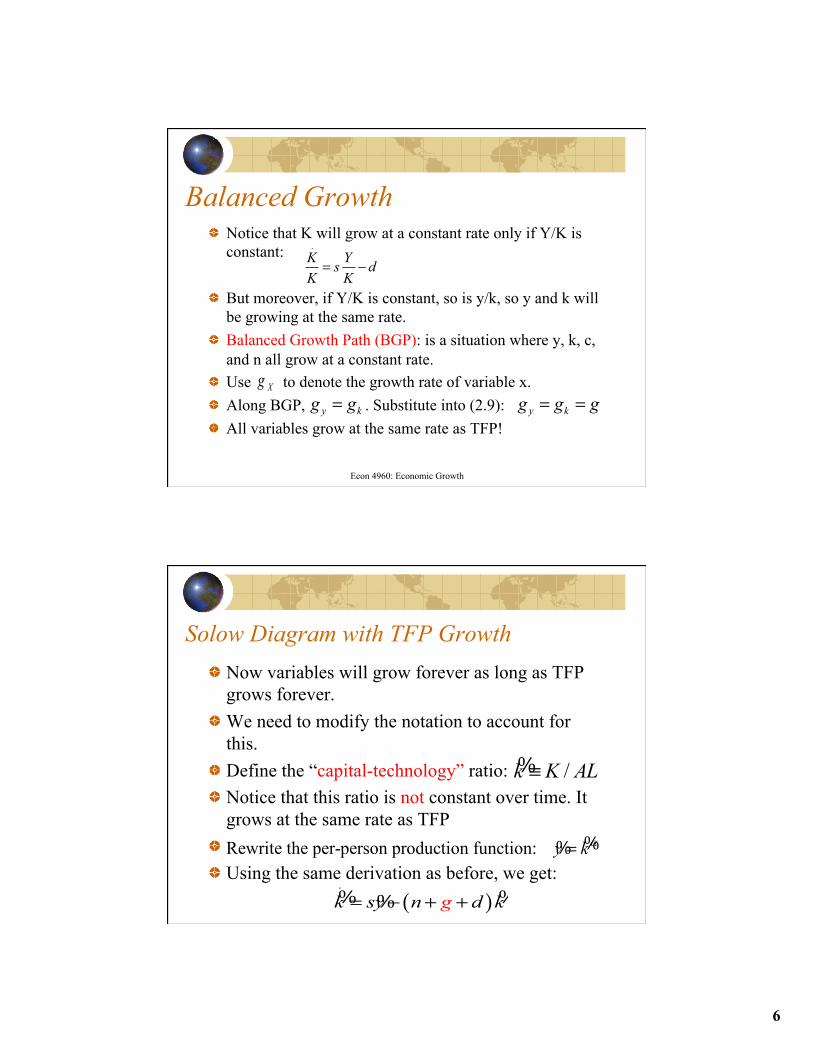
Balanced Growth !   Notice that K will grow at a constant rate only if Y/K is

constant:

!   But moreover, if Y/K is constant, so is y/k, so y and k will be growing at the same rate.

!   Balanced Growth Path (BGP): is a situation where y, k, c, and n all grow at a constant rate.

!   Use to denote the growth rate of variable x. !   Along BGP, . Substitute into (2.9): !   All variables grow at the same rate as TFP!


.K Ys dK K

= −

Xgy kg g= y kg g g= =

Solow Diagram with TFP Growth !  Now variables will grow forever as long as TFP

grows forever. !  We need to modify the notation to account for

this. !  Define the “capital-technology” ratio: !  Notice that this ratio is not constant over time. It

grows at the same rate as TFP !   !  Using the same derivation as before, we get:

/k K AL≡%

Rewrite the per-person production function: y kα= %%

( ).

k s n gy d k= − + +% %%

7

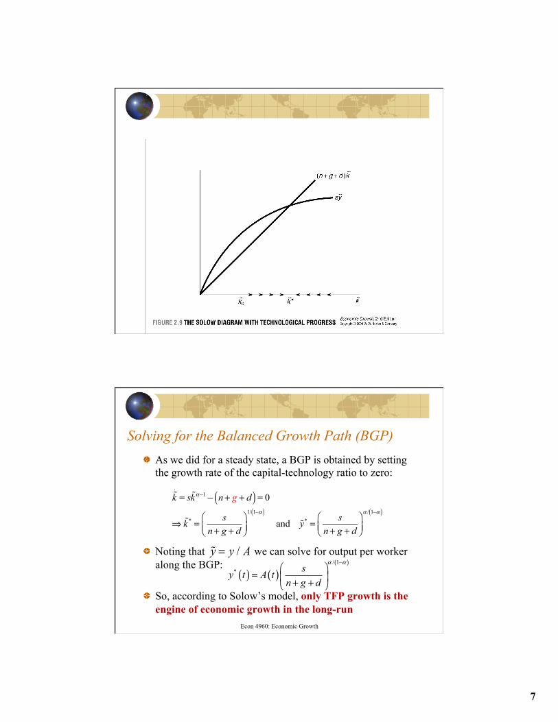
Fig. 2.9

Solving for the Balanced Growth Path (BGP) !   As we did for a steady state, a BGP is obtained by setting

the growth rate of the capital-technology ratio to zero:

!   Noting that we can solve for output per worker along the BGP:

!   So, according to Solow’s model, only TFP growth is the engine of economic growth in the long-run


k.

= s kα−1 − n+ g + d( ) = 0

⇒ k * = sn+ g + d

⎛⎝⎜

⎞⎠⎟

1/ 1−α( ) and y* = s

n+ g + d⎛⎝⎜

⎞⎠⎟

α / 1−α( )

y = y / A

( ) ( )( )/ 1

* sy t A tn g d

α α−⎛ ⎞

= ⎜ ⎟+ +⎝ ⎠

8

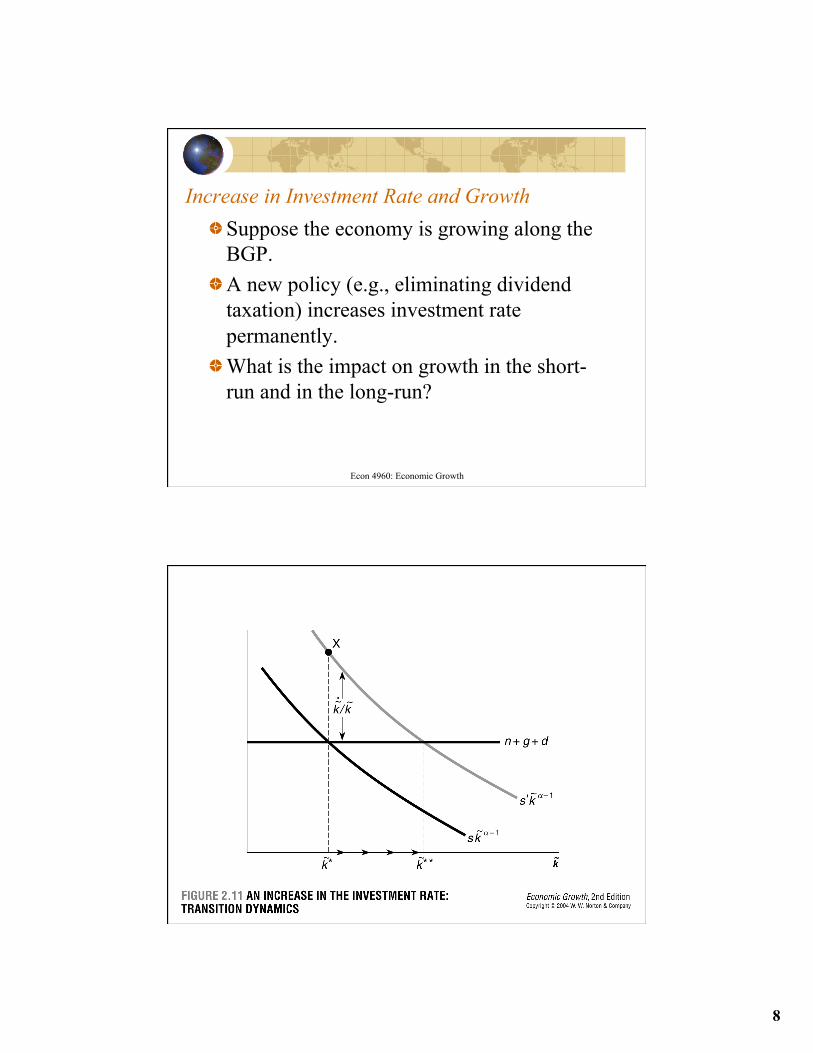
Increase in Investment Rate and Growth !  Suppose the economy is growing along the

BGP. !  A new policy (e.g., eliminating dividend

taxation) increases investment rate permanently.

!  What is the impact on growth in the short-run and in the long-run?


Fig. 2.11

9

Fig. 2.12

Fig. 2.13

10

Level versus Growth Rate Effects !   If a comparative static exercise results in a permanent shift

in the level of output, we call this a “level effect.” !   If it permanently increases the growth rate, we call this a

“growth rate effect.” !   Which one is more important (or better)? !   It generally depends: do you prefer your income to double

tomorrow or its growth rate to change by 0.1%? !   Among other things it also depends on time preference or

patience. !   But growth rate effects compound over time and can

potentially have huge effects in the long-run, so the distinction between the two types of effects should be kept in mind Econ 4960: Economic Growth

GROWTH ACCOUNTING


11

Growth Accounting !   Use the same identity we derived before. Define !   For total output:

!   For output per person:

!   Both versions will come in handy depending on the question we have in mind


+y B ky B k

α=g g g

1B A α−=

( ) + 1Y B K LY B K L

α α= + −g g g g

22

FIGURE 4-11a Contribution to total output growth 1913–1950.

12

23

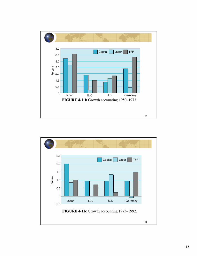
FIGURE 4-11b Growth accounting 1950–1973.

24

FIGURE 4-11c Growth accounting 1973–1992.

13

25

FIGURE 4-12 Growth accounting in emerging markets, 1960–1994.

Global Business Environment 26

Growth Accounting for the United States Output Labor Capital TFP

60’s70’s80’s90’s

4.1%3.23.03.3

1.5%2.11.71.1

3.4%3.72.91.9

1.4%0.10.51.7

For labor and capital contributions to growth in output – multiply by shares

14

Global Business Environment 27

In The News White House Struggles to Halt Flap Over Jobs

Report (Reuters, Feb 19th, 2004) “The White House on Thursday struggled anew to contain the fallout over an overly optimistic forecast that 2.6 million jobs will be created this year and some Republicans expressed concern about the damage being done to President Bush … ‘We are eager for some reassurance that your economic projections and estimates are based in reality, not political fiction,’ said the letter, signed by House Democratic leader Nancy Pelosi and others.”

28

The President’s Forecast

15

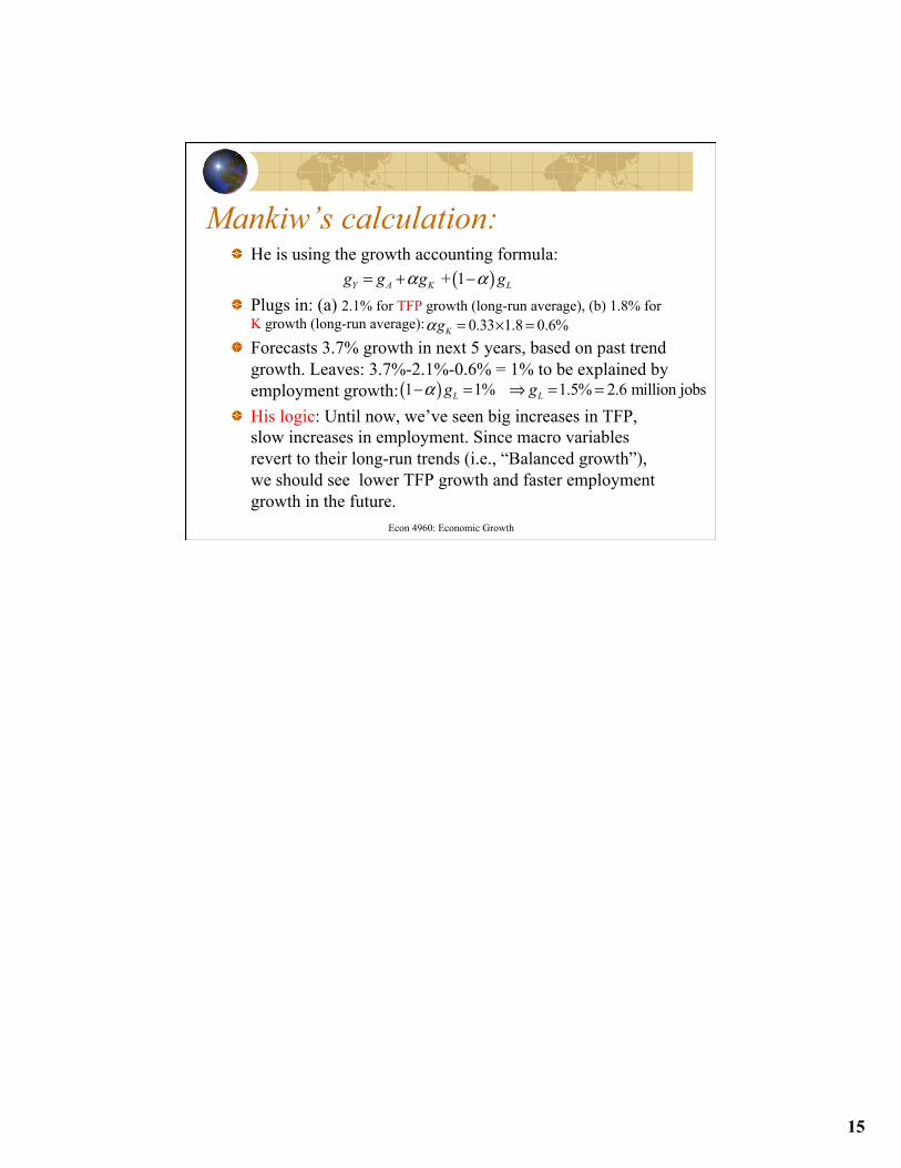
Mankiw’s calculation: !   He is using the growth accounting formula: !   Plugs in: (a) 2.1% for TFP growth (long-run average), (b) 1.8% for

K growth (long-run average):

!   Forecasts 3.7% growth in next 5 years, based on past trend growth. Leaves: 3.7%-2.1%-0.6% = 1% to be explained by employment growth:

!   His logic: Until now, we’ve seen big increases in TFP, slow increases in employment. Since macro variables revert to their long-run trends (i.e., “Balanced growth”), we should see lower TFP growth and faster employment growth in the future.


( ) + 1 Y A K Lg g g gα α= + −

0.33 1.8 0.6%Kgα = × =

( )1 1% 1.5% 2.6 million jobsL Lg gα− = ⇒ = =

technology and the solow model - university of …users.econ.umn.edu/~guvenen/lecture5.pdf1...

Documents