Telco Churn Prediction with Big Data

Yiqing Huang1,2, Fangzhou Zhu1,2, Mingxuan Yuan3, Ke Deng4, Yanhua Li3, Bing Ni3,Wenyuan Dai3, Qiang Yang3,5, Jia Zeng1,2,3,∗

1School of Computer Science and Technology, Soochow University, Suzhou 215006, China2Collaborative Innovation Center of Novel Software Technology and Industrialization

3Huawei Noah’s Ark Lab, Hong Kong4School of Computer Science and Information Technology, RMIT University, Australia

5Department of Computer Science and Engineering, Hong Kong University of Science and Technology∗Corresponding Author: zeng.jia@acm.org

ABSTRACTWe show that telco big data can make churn prediction muchmore easier from the 3V’s perspectives: Volume, Variety,Velocity. Experimental results confirm that the predictionperformance has been significantly improved by using a largevolume of training data, a large variety of features from bothbusiness support systems (BSS) and operations support sys-tems (OSS), and a high velocity of processing new comingdata. We have deployed this churn prediction system in oneof the biggest mobile operators in China. From millions ofactive customers, this system can provide a list of prepaidcustomers who are most likely to churn in the next month,having 0.96 precision for the top 50000 predicted churners inthe list. Automatic matching retention campaigns with thetargeted potential churners significantly boost their rechargerates, leading to a big business value.

Categories and Subject DescriptorsH.4 [Information Systems Applications]: Miscellaneous;H.2.8 [Database Management]: Database Applications—Data Mining

KeywordsTelco churn prediction; big data; customer retention

1. INTRODUCTIONCustomer churn is perhaps the biggest challenge in telco

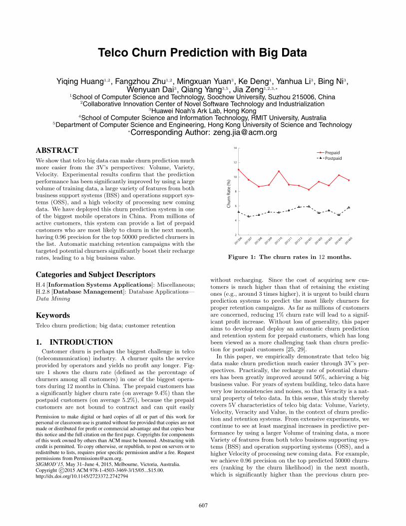
(telecommunication) industry. A churner quits the serviceprovided by operators and yields no profit any longer. Fig-ure 1 shows the churn rate (defined as the percentage ofchurners among all customers) in one of the biggest opera-tors during 12 months in China. The prepaid customers hasa significantly higher churn rate (on average 9.4%) than thepostpaid customers (on average 5.2%), because the prepaidcustomers are not bound to contract and can quit easily

Permission to make digital or hard copies of all or part of this work forpersonal or classroom use is granted without fee provided that copies are notmade or distributed for profit or commercial advantage and that copies bearthis notice and the full citation on the first page. Copyrights for componentsof this work owned by others than ACM must be honored. Abstracting withcredit is permitted. To copy otherwise, or republish, to post on servers or toredistribute to lists, requires prior specific permission and/or a fee. Requestpermissions from Permissions@acm.org.SIGMOD’15, May 31–June 4, 2015, Melbourne, Victoria, Australia.Copyright c©2015 ACM 978-1-4503-3469-3/15/05...$15.00.http://dx.doi.org/10.1145/2723372.2742794

2013062

4

6

8

10

12

14

Chur

n Ra

te (%

)

PrepaidPostpaid

201312

201311

201310

201309

201308

201307

201405

201404

201403

201402

201401

Figure 1: The churn rates in 12 months.

without recharging. Since the cost of acquiring new cus-tomers is much higher than that of retaining the existingones (e.g., around 3 times higher), it is urgent to build churnprediction systems to predict the most likely churners forproper retention campaigns. As far as millions of customersare concerned, reducing 1% churn rate will lead to a signif-icant profit increase. Without loss of generality, this paperaims to develop and deploy an automatic churn predictionand retention system for prepaid customers, which has longbeen viewed as a more challenging task than churn predic-tion for postpaid customers [25, 29].

In this paper, we empirically demonstrate that telco bigdata make churn prediction much easier through 3V’s per-spectives. Practically, the recharge rate of potential churn-ers has been greatly improved around 50%, achieving a bigbusiness value. For years of system building, telco data havevery low inconsistencies and noises, so that Veracity is a nat-ural property of telco data. In this sense, this study therebycovers 5V characteristics of telco big data: Volume, Variety,Velocity, Veracity and Value, in the context of churn predic-tion and retention systems. From extensive experiments, wecontinue to see at least marginal increases in predictive per-formance by using a larger Volume of training data, a moreVariety of features from both telco business supporting sys-tems (BSS) and operation supporting systems (OSS), and ahigher Velocity of processing new coming data. For example,we achieve 0.96 precision on the top predicted 50000 churn-ers (ranking by the churn likelihood) in the next month,which is significantly higher than the previous churn pre-

607

diction system deployed in this operator (0.68 precision) aswell as the current state-of-the-art research work [16, 14, 13,32, 1].1 The results are based on the 9-month dataset fromaround two million prepaid customers in one of the biggestoperators in China. This study provides a clear illustra-tion that bigger data indeed can be more valuable assetsfor improving generalization ability of predictive modelinglike churn prediction. Moreover, the results suggest that itis worthwhile for telco operators to gather both more datainstances and more possible data features, plus the scal-able computing platform to take advantage of them. In thissense, the big data platform plays a major role in the next-generation telco operation. As an additional contribution,we introduce how to integrate churn prediction model withretention campaign systems, automatically matching properretention campaigns with potential churners. In particular,the churn prediction model and the feedback of retentioncampaign form a closed loop in feature engineering.

To summarize, this paper makes two main contributions.The primary contribution is an empirical demonstration thatindeed churn prediction performance can be significantly im-proved with telco big data by integrating both BSS and OSSdata. Although BSS data have been utilized in churn pre-diction very well in the past decade, we have shown thatit is worthwhile collecting, storing and mining OSS data,which takes around 97% size of the entire telco data assets.This churn prediction system is one of the important com-ponents for the deployed telco big data platform in one ofthe biggest operators, China. The second contribution isthe integration of churn prediction with retention campaignsystems as a closed loop. After each campaign, we knowwhich potential churners accept the retention offers, whichcan be used as class labels to build a multi-class classifierautomatically matching proper offers with churners. Thismeans that we can use a reasonable campaign cost to makethe most profit. This paper thereby makes a small but im-portant addition to the cumulative answer to a current openindustrial question: How to monetize telco big data?

2. PREVIOUS WORKIn industry, data-driven churn predictive modeling gen-

erally includes constructing useful features (aka predictorvariables) and building good classifiers (aka predictors) orclassifier ensembles with these features [13, 36]. A binaryclassifier is induced from instances of training data, for whichthe class labels (churners or non-churners) are known. Usingthis classifier, we want to predict the class labels of instancesof test data in the near future, where training and test datahave no overlap in time intervals. Each instance typically isdescribed by a vector of features which will be used for pre-diction. Following this research line, many classifiers havebeen adopted for churn prediction, including logistic regres-sion [24, 14, 22, 25, 23], decision trees [34, 22, 3], boost-ing algorithms (e.g., variants of adaboost [18, 23]), boostedtrees (gradient boosted decision trees) or random forest [21,27], neural networks [9, 16], evolutionary computation (e.g.,genetic algorithm and ant colony optimization) [9, 2, 33],ensemble of support vector machines [7, 33, 20], and en-

1Although we cannot fairly compare our results with previ-ous results due to different datasets, features and classifiers,we enhance the predictive performance over baselines thatare adopted by most of previous research work.

Data Intergration/ETL/Pretreatment

Big Data Modeling & Mining

Data Bus

Capability Bus

DataResources

Big DataPlatform

ApplicationsLayer

HadoopHiveSpark SQLDat

a La

yer

Capa

bilit

y La

yer

Data SourceIncrement

(Day)

TotalUser BaseBehavior Compliant Billing Voice/SMS

CDR CS PS MR

4.1G 0.8G 0.8G 18.3G 34G 1.0T 1.2T 2.3T

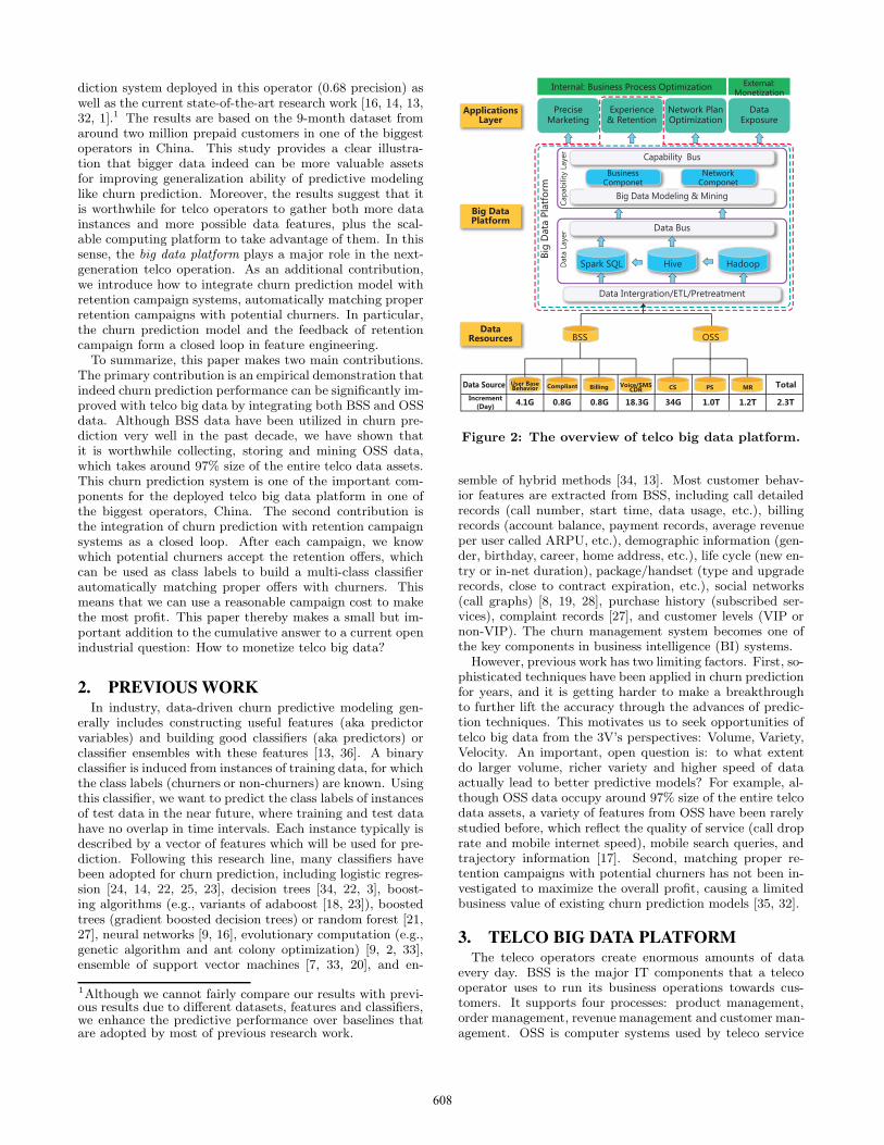
Figure 2: The overview of telco big data platform.

semble of hybrid methods [34, 13]. Most customer behav-ior features are extracted from BSS, including call detailedrecords (call number, start time, data usage, etc.), billingrecords (account balance, payment records, average revenueper user called ARPU, etc.), demographic information (gen-der, birthday, career, home address, etc.), life cycle (new en-try or in-net duration), package/handset (type and upgraderecords, close to contract expiration, etc.), social networks(call graphs) [8, 19, 28], purchase history (subscribed ser-vices), complaint records [27], and customer levels (VIP ornon-VIP). The churn management system becomes one ofthe key components in business intelligence (BI) systems.

However, previous work has two limiting factors. First, so-phisticated techniques have been applied in churn predictionfor years, and it is getting harder to make a breakthroughto further lift the accuracy through the advances of predic-tion techniques. This motivates us to seek opportunities oftelco big data from the 3V’s perspectives: Volume, Variety,Velocity. An important, open question is: to what extentdo larger volume, richer variety and higher speed of dataactually lead to better predictive models? For example, al-though OSS data occupy around 97% size of the entire telcodata assets, a variety of features from OSS have been rarelystudied before, which reflect the quality of service (call droprate and mobile internet speed), mobile search queries, andtrajectory information [17]. Second, matching proper re-tention campaigns with potential churners has not been in-vestigated to maximize the overall profit, causing a limitedbusiness value of existing churn prediction models [35, 32].

3. TELCO BIG DATA PLATFORMThe teleco operators create enormous amounts of data

every day. BSS is the major IT components that a telecooperator uses to run its business operations towards cus-tomers. It supports four processes: product management,order management, revenue management and customer man-agement. OSS is computer systems used by teleco service

608

providers to manage their networks (e.g., mobile networks).It supports management functions such as network inven-tory, service provisioning, network configuration and faultmanagement. Note that both BSS and OSS often work sep-arately, and have their own data and service responsibilities,With the rapid expansion, the telco data storage has movedto PB age, which requires a scalable big data computingplatform for monetization.

Figure 2 overviews the functional architecture of the telcobig data platform, where data sources are from both BSSand OSS. Generally, the data from BSS are composed ofUser Base/Behavior, Compliant, Billing and Voice/Messagecall detailed records (CDR) tables, which cover users’ de-mographic information, package, call times, call duration,messages, recharge history, account balance, calling num-ber, cell tower ID, and complaint records. The data volumein BSS is around 24GB per day. The data from OSS canbe broadly categorized into three parts: circuit switch (CS),packet switch (PS) and measurement report (MR). CS datadescribe the call connection quality, e.g., call drop rate andcall connection success rate. PS data are often called mobilebroadband (MBB) data, including data gathered by probesusing Deep Packet Inspection (DPI). PS data describe users’mobile web behaviors, which is related to web speed, connec-tion success rate, and mobile search queries. MR data arefrom radio network controller (RNC), which can be used toestimate users’ approximate trajectories [17]. The data vol-ume in OSS is around 2.2TB per day, occupying over 97%data volume of the entire dataset. Also, we can use webcrawler to obtain some Internet data (e.g., map informationand social networks).

More specifically, BSS data are from the traditional BIsystems widely used in telco operators, which consist ofaround 140 tables. OSS data are imported by the Huawei in-tegrated solution called SmartCare, which collects the datafrom probes and interpret them to x-Detail Record (xDR)tables, such as User Flow Detail Record (UFDR), Trans-action Detail Record (TDR), and Statistics Detail Record(SDR). All these tables have the key value called Interna-tional Mobile Subscriber Identification Number (IMSI) orInternational Mobile Equipment Identity (IMEI), which canbe used for joint operation and feature engineering. We usethe multi-vendor data adaption module to change tables tothe standard format, which are imported to big data plat-form through extract-transform-load (ETL) tools for dataintegration. We store these raw tables in Hadoop distributedfile systems (HDFS), which communicates with Hive/SparkSQL for feature engineering purposes. These compose thedata layer connected with the capability layer through thedata bus in the big telco data platform. The main workloadof data layer is to collect and update all tables from BSSand OSS periodically. In the capability layer, we build twotypes of models, business and network components, based onboth unlabeled and labeled instances of features using datamining and machine learning algorithms. Using capabilitybus, these models can support application layer including in-ternal (e.g., precise marketing, experience & retention andnetwork plan optimization) and external applications (e.g.,data exposure for trading). The main workloads of applica-tion layer include customer insight (e.g., churn, complaint,recommendation products or services) and network insight(e.g., network planning and optimization). The churn pre-

HDFS

Apache Spark

Feature Engineering

Classifiers

Rete

ntio

n Ca

mpa

igns

Figure 3: Churn prediction and retention systems.

diction system is supported by the telco big data platform,and is located at the red dashed lines in Figure 2.

Efficient management of telco big data for predictive mod-eling poses a great challenge to the computing platform [11].For example, there are around 2.3TB new coming data perday from both BSS and OSS sources, where more than97% volume of data is from OSS. The empirical results arebased on a scalable churn prediction and retention systemusing Apache Hadoop [31] and Spark [37] distributed ar-chitectures including three key components: 1) data gath-ering/integration, 2) feature engineering/classifiers, and 3)retention campaign systems. In the data gathering and in-tegration, we move data tables from different sources andintegrate some tables by ETL tools. Most data are storedin regular tables (e.g., billing and demographic information)or sparse matrix (e.g., unstructured information like textualcomplaints, mobile search queries and trajectories) in HDFS.The feature engineering and classification components arehand coded in Spark, which is based on Hive/Spark SQLand some widely-used unsupervised/supervised learning al-gorithms, including PageRank [26], label propagation [40],topic models (latent Dirichlet allocation or LDA) [4, 39], LI-BLINEAR (L-2 regularized logistic regression) [12], LIBFM(factorization machines) [30], gradient boosted decision tree(GBDT) and random forest (RF) [5]. This churn manage-ment platform has been deployed in the real-world operator’ssystems, which can scale up efficiently to massive data fromboth BSS and OSS.

4. PREDICTION AND RETENTIONThe structure of the churn prediction system is illustrated

in Figure 3. The HDFS and Apache Spark support the dis-tributed storage and management of raw data. Feature en-gineering techniques are applied to select and extract rele-vant features for churn model training and prediction. Inthe business period (monthly), the churn classifier providesa list of likely churners for proper retention campaigns. Inparticular, the churn prediction model and the feedback ofretention campaign form a closed-loop.

4.1 Feature EngineeringWe make use of Hive and Spark SQL to quickly sanitize

the data and extract the huge amount of useful features. Theraw data are stored on HDFS as Hive tables. Because Hiveruns much slower than Spark SQL, we use Spark SQL tomanipulate the tables. Spark SQL is a new SQL engine de-signed from ground-up for Spark.2 It brings native supportfor SQL to Spark and streamlines the process of queryingdata stored both in RDD (Resilient Distributed Dataset)and Hive [37]. The Hive tables are directly imported into

2https://spark.apache.org/sql/

609

Features Description Features Description

localbase outer call dur duration of local-base outer call ld call dur duration of long-distance callroam call dur duration of roaming call localbase called dur duration of local-base calledld called dur duration of long-distance called roam called dur duration of roaming calledcm dur duration of calling China Mobile ct dur duration of calling China Telecombusy call dur duration of calling in busy time fest call dur duration of calling in festivalsms p2p inner mo cnt count of inner-net MO SMS sms p2p other mo cnt count of other MO SMSsms p2p cm mo cnt count of MO SMS with China Mobile sms p2p ct mo cnt count of MO SMS with China Telecomsms info mo cnt count of information-on-demand MO SMS sms p2p roam int mo cnt count of roaming international MO SMSmms p2p inner mo cnt count of inner-net Mo MMS mms p2p other mo cnt count of other MO MMSmms p2p cm mo cnt count of MO MMS with China Mobile mms p2p ct mo cnt count of MO MMS with China Telecommms p2p roam int mo cnt count of roaming international MO MMS all call cnt count of all callvoice cnt count of voice call local base call cnt count of local-base callld call cnt count of long-distance call roam call cnt count of roaming callcaller cnt count of caller call voice dur duration of voice callcaller dur duration of caller call localbase inner call dur duration of local-base inner-net callfree call dur duration of free call call 10010 cnt count of call to 10010 (service number)call 10010 manual cnt count of call to manual 10010 sms bill cnt count of billing SMSsms p2p mt cnt count of MT SMS mms cnt count of all MMSmms p2p mt cnt count of MT MMS gprs all flux all GPRS fluxgender gender of user age age of usercredit value user credit value innet dura duration of innettotal charge the total cost in a month gprs flux the total GPRS fluxgprs charge the total cost of GPRS local call minutes minutes of local calltoll call minutes minutes of long-distance call roam call minutes minutes of roaming callvoice call minutes minutes of voice call p2p sms mo cnt count of MO SMSp2p sms mo charge cost of MO SMS pspt type credentials typeis shanghai if user is shanghai resident or not town id user town idsale id selling area id pagerank user effect calculated with pagerankproduct id product id product price product priceproduct knd kind of product gift voice call dur duration of gift voice callgift sms mo cnt count of gift MO SMS gift flux value gift fluxdistinct serve count count of service SMS serve sms count count of service provider through SMSinnet dura duration in net balance account balancebalance rate recharge over account balance total charge recharge valuePAGESIZE page size PAGE SUCCEED FLAG page display success flagL4 UL THROUGHPUT data upload speed L4 DW THROUGHPUT data download speedTCP CONN STATES TCP connection status TCP RTT TCP return timeSTREAMING FILESIZE streaming file size STREAMING DW PACKETS streaming download packetsALERTTIME alert time ENDTIME alert end timeLAC local area code CI cell ID

Figure 4: Some basic features in churn prediction.

Spark SQL for basic queries, including join queries and ag-gregation queries. For example, we need to join the localcall table and the roam call table to combine the local calland roam call features. Also, we need to aggregate localcall tables of different days to summarize a customer’s callinformation in a time period (e.g., a month). All the in-termediate results are stored as Hive tables, which can bereused by other tasks since the feature engineering may berepeated many times. Finally, a unified wide table is gener-ated, where each tuple in the table represents a customer’sfeature vector. The wide table is exported into Hive to buildclassifiers. An example of some basic features in the widetable and explanations can be found in Figure 4.

These basic features can be broadly categorized into threeparts: 1) baseline features, 2) CS features, and 3) PS fea-tures. The baseline features are extracted from BSS andare used in most previous research work, e.g., account bal-ance, call frequency, call duration, complaint frequency, datausage, recharge amount, and so on. We use these base-line features to illustrate the differences between our solu-tion and previous work. These features compose a vector,xm = [x1, . . . , xi, . . . , xj , . . . , xN ], for each customer m.

Besides these basic features, we also use some unsuper-vised, semi-supervised and supervised learning algorithms toextract the following complicated features: 1) Graph-basedFeatures, 2) Topic Features, and 3) Second-order Features.

4.1.1 CS and PS FeaturesBoth CS and PS features are from OSS. We use several

key performance indicators (KPI) and key quality indica-

tors (KQI) in OSS as well as some statistical features, suchas the average data upload/download speed and the mostfrequent connection locations from MR data. Due to thepage limitation and the focus of this paper, we only give abrief introduction of the KPI/KQI features extracted fromCS/PS data. Interested users can check Huawei’s industrialOSS handbook for details.3

CS features represent the service quality of voice. TheKPI/KQI features used in CS data includes average Per-ceived Call Success Rate, average E2E Call Connection De-lay, average Perceived Call Drop Rate and average VoiceQuality. Perceived Call Success Rate indicates the call suc-cess rate perceived by a calling customer. It is calculatedfrom the formula, [Mobile Originated Call Alerting]/([MobileOriginated Call Attempt] + [Immediate Assignment Fail-ures]/2). Each item in the formula is computed from a groupof PIs (performance indicators). E2E Call Connection De-lay indicates the amount of time a calling customer waitsbefore hearing the ringback tone. It is defined as [E2E CallConnection Total Delay]/[Mobile Originated Call Alerting]= [Sum(Mobile Originated Connection Time - Mobile Orig-inated Call Time)]/[Mobile Originated Call Alerting]. Per-ceived Call Drop Rate indicates the call drop rate perceivedby a customer. It is obtained from [Radio Call Drop AfterAnswer]/[Call Answer]. Voice quality include Uplink MOS(Mean Opinion Score), Downlink MOS, IP MOS, One-wayAudio Count, Noise Count, and Echo Count. They can beused to assess the voice quality in the operator’s network

3HUAWEI SEQ Analyst KQI&KPI Definition

610

and the customers’ experience of voice services. Totally,each customer has a total of 9 CS KPI/KQI features.

PS KPI/KQI features reflect the quality of data service,which includes web, streaming and email. For example, weuse the web features such as average Page Response SuccessRate, average Page Response Delay, average Page BrowsingSuccess Rate, average Page Browsing Delay, and averagePage Download Throughput. Page Response Success Rateindicates the rate at which website access requests are suc-cessfully responded to after the customer types a UniformResource Locator (URL) in the address bar of a web browser.It is calculated from [Page Response Successes]/[Page Re-quests], where [Page Response Successes] = [First GET Suc-cesses] and [Page Requests] = [First GET Requests]. PageResponse Delay indicates the amount of time a customerwaits before the desired web page information starts to dis-play in the title bar of a browser after the customer typesa URL in the address bar. It is obtained from [Total PageResponse Success Delay]/[Page Response Successes], where[Page Response Success Delay] = [First GET Response Suc-cess Delay] + [First TCP Connect Success Delay]. SimilarKPI/KQI features are used for both streaming and email ser-vices. For each customer, we also select top 5 most frequentlocations or stay areas during a period (e.g., a month) repre-sented by latitude and longitude from MR data. Therefore,each customer has 15 PS KPI/KQI features plus 10 mostfrequent location features from PS data.

4.1.2 Graph-based FeaturesGraph-based features are extracted from the call graph,

message graph and co-occurrence graph, based on CDR andMR data. All are undirected graphs with nodes for cus-tomers. The edge weight of call and message graphs arethe accumulated mutual calling time and the total num-ber of messages between two customers in a fixed period(e.g., a month) from CDR data. The edge weight of co-occurrence graph is the number of co-occurrences of two cus-tomers within a certain spatiotemporal cube (e.g., within 20minute and 100×100 meter cube) from MR data. Churnerswill propagate their information through these graphs.

We use Hive/Spark SQL to generate the above undirectedgraphs represented by the edge-based sparse matrix, E ={wm,n �= 0}, where wm,n �= 0 is the edge weight for mthand nth vertices (customers), and there are a total of 1 ≤m, n ≤ N customers. Based on the undirected graphs, weuse PageRank [26] and label propagation [40] algorithms toproduce two features for each graph. The weighted PageR-ank feature xm on undirected graphs is calculated as follows,

xm =(1− d)

N+ d

∑

n∈N (m)

xnwm,n∑n∈N (m) wm,n

, (1)

whereN (m) is the set of neighboring customers having edgeswith m. The damping factor d is set to 0.85 practically. Theinitial value of xm = 1. After several iterations of Eq. (1),xm will converge to a fixed point due to random walk na-ture of the PageRank algorithm. The higher value of xm

corresponds to the higher importance in the graph. For ex-ample, in the call graph, the higher xm of a customer meansthat more customers call (or called) this customer. Intu-itively, customers with higher xm have a low likelihood tochurn. Each customer has a total of 3 PageRank features on3 undirected graphs.

In label propagation, the basic idea is that we start with

a group of customers that we have known that they arechurners. Following the edge weights in the graph, we propa-gate the churner probabilities from the customer seed vertex(the ones we have churner label information about) into thecustomers without churner labels. After several iterations,the label propagation algorithm converges and the outputis churner labels for the non-churner customers. Given theedge weight matrix WM×M , and a churner label probabilitymatrix YM×2, the label propagation algorithm follows the 3iterative steps:

1. Y ←WY ;

2. Row-normalize Y to sum to 1;

3. Fix the churner labels in Y , Repeat from Step 1 untilY converges.

After label propagation, each customer (non-churner) is as-sociated with a churn label probability ym in matrix Y prop-agated from the churners in the previous month. The highervalue means that this non-churner has a higher likelihood tobe the churner in the graph. Since we have 3 undirectedgraphs, we obtain 3 churner label propagation features ym

for each customer m. As a result, we have 6 graph-based fea-tures for each customer plus 3 PageRank features, which aredifferent and independent from label propagation featuresbecause PageRank features do not involve churner labels.

4.1.3 Topic FeaturesThere are lots of text logs of customer complaints or search

queries. In a certain period (e.g., a month), each customercan be represented as a document containing a bag of wordsof their complaint or search text. After removing less fre-quent words, we form 2408 and 15974 vocabulary words fromcomplaint and search text. Because the word vector spaceis too sparse and high-dimensional to build a RF classi-fier, we choose the probabilistic topic modeling algorithmcalled LDA [4] to obtain compact and lower-dimensionaltopic features. We use a sparse matrix xW×M to repre-sent the bag-of-word representation of all customers, wherethere are 1 ≤ m ≤ M customers and 1 ≤ w ≤ W vocabu-lary words. LDA allocates a set of thematic topic labels, z ={zk

w,m}, to explain non-zero elements in the customer-wordco-occurrence matrix xW×M = {xw,m}, where 1 ≤ w ≤ Wdenotes the word index in the vocabulary, 1 ≤ m ≤ Mdenotes the document index, and 1 ≤ k ≤ K denotes thetopic index. Usually, the number of topics K is provided byusers. The nonzero element xw,m �= 0 denotes the numberof word counts at the index {w, m}. The objective of LDAinference algorithms is to infer posterior probability fromthe full joint probability p(x, z, θ, φ|α, β), where z is thetopic labeling configuration, θK×M and φK×W are two non-negative matrices of multinomial parameters for document-topic and topic-word distributions, satisfying

∑k θm(k) = 1

and∑

w φw(k) = 1. Both multinomial matrices are gener-ated by two Dirichlet distributions with hyperparameters αand β. For simplicity, we consider the smoothed LDA withfixed symmetric hyperparameters.

We use a coordinate descent (CD) method called beliefpropagation (BP) [38, 39] to maximize the posterior proba-bility of LDA,

p(θ, φ|x, α, β) =p(x,θ, φ|α, β)

p(x|α, β)∝ p(x,θ, φ|α, β). (2)

611

The output of LDA contains two matrices {θ, φ}. In prac-tice, the number of topics K in LDA is set to 10. Thematrix θK×M is the low-dimensional topic features for allcustomers, when compared with the original sparse high-dimensional matrix xW×M because K � D. For both com-plaint and search texts, we generate K = 10 dimensionaltopic features of each customer, respectively. So, there area total of 20 topic features for each customer.

4.1.4 Second-order FeaturesIn the feature vector, xm = [x1, . . . , xi, . . . , xj , . . . , xN ],

second-order features are defined as the product of any twofeature values xixj , which may help us find the hidden re-lationship between a specific pair of features. Suppose thatthere are N features, the total number of second-order fea-tures could be (N +1)N/2, which is often a burden to builda classifier. So, we use LIBFM [30] regression model to se-lect the most useful second-order features. The regressionmodel can be used for classification problems by setting theresponse of regression as class labels. The LIBFM optimizesthe following objective function by the stochastic gradientdescent algorithm,

y = w0 +n∑

i=1

wixi +n∑

i=1

n∑

j=i+1

〈vi,vj〉xixj , (3)

where w0 and wi are weight parameters, and vi is a K-lengthvector for ith feature value. The inner product 〈vi,vj〉 de-notes the weight for the second-order feature xixj . Thelarger weight means that the second-order feature is moreimportant [30]. So, we rank the learned weight 〈vi, vj〉 afteroptimizing (3), and select 20 second-order features with thetop largest weights for churn prediction.

4.2 ClassifiersFor experiments we report, we choose the Random Forest

(RF) classifier [5] to make predictions. The major reason ofthis choice is that RF yields the best predictive performanceamong several widely-used classifiers (See comparisons inSubsection 5.8). RF is a supervised learning method thatuses the bootstrap aggregating (bagging) technique for anensemble of decision trees. Given a set of training instances,xm = [x1, . . . , xi, . . . , xj , . . . , xN ], with class labels ym ={non-churner = 0, churner = 1}, RF fits a set of decisiontrees ft, 1 ≤ t ≤ T to the random subspace of features.The label prediction for test instance x is the average of thepredictions from all individual trees,

y =1

T

T∑

t=1

ft(x), (4)

where y is the likelihood of being a churner. We rank thislikelihood in descending order for predictive performanceevaluation as well as for retention campaigns. Generally,customers with higher likelihood have lower recharge ratesin our experiments.

For each decision tree, it randomly selects a subset of√

Nfrom N features, and builds a splitting node by iteratingthese features. The Gini improvement I(·) is used to deter-mine the best splitting point given ith column of features

from xM×N ,

I(x1:M,i) = G(x1:M,i)− q ×G(x1:P,i)

−(1− q)×G(xP+1:M,i), (5)

G(·) = 1−2∑

c=1

p2c, (6)

where P is the splitting point that partition 1 : M instancesinto two parts 1 : P and P + 1 : M , and q is the fraction ofinstances going left to the splitting point P . The functionG(·) is the Gini index for a group of customer instances, andp1 is the probability of churners and p2 is the probability ofnon-churners in this group. For each column of features,we visit all splitting points P and find the maximum Giniimprovement I . Then, we find the maximum I among allfeatures, and use the feature with the maximum I as thesplitting point in the node of a decision tree. Other parame-ters of RF are given as follows: 1) the number of trees is 500and 2) the minimum samples in leaf nodes is 100. We fix theminimum samples in leaf nodes to 100 to avoid over-fitting.The split process of each decision tree will stop when thenumber of samples in an individual node is less than 100.

After training RF, we obtain each feature’s importancevalue by summing the Gini improvements of all nodes,

Importancei =T∑

t=1

∑

Pi∈treet

I(x1:M,i). (7)

The feature importance ranking could help us evaluate whichfeatures are major factors in churn prediction.

4.3 Retention SystemsThe retention systems for potential churners make a closed

loop with churn prediction systems as shown in Figure 3.Telco operators are not only concerned with the potentialchurners, but also want to carry out effective retention cam-paigns to retain those potential churners for further profits.Generally, if a customer accept a retention offer, he/she willkeep on using the operator’s service for the next 5 monthsto get the 1/5 offer per month. Nevertheless, there are mul-tiple retention offers and operators do not know which offersmatch a specific group of potential churners. For example,some potential churners will not accept any offer, some wantmore cashback, some want more flux, and some want morefree voice minutes. Before the automatic retention system isdeployed, operators often match offers with potential churn-ers by domain knowledge, and the campaign results are notsatisfactory. So, it is necessary to build an automatic reten-tion systems for matching offers with churners.

We define this task as a multi-category classification prob-lem. A potential churner xm is classified into multiple cat-egories ym = {0, 1, 2, . . . , C − 1}, where ym = 0 denotesthat the potential churner will not accept any offer, andother values means different types of retention offers. Theclass labels (retention results) are accumulated after eachretention campaign. We train a RF retention classifier inSubsection 4.2 to do multi-category classification as shownin Figure 3. The retention classifier is updated if retentioncampaign results are available, similar to the churn classi-fier. Moreover, we use the label propagation algorithm topropagate the campaign result label ym on three undirectedgraphs in Subsection 4.1.2. These 3 × C new features areadded to the original churn prediction features for training

612

1 10 20 300

10

20

30

40

50

Days

Num

ber o

f cus

tom

ers

×10

4

Figure 5: Distribution of the number of rechargedcustomers in the recharge period.

Month (N) Month (N+1) Month (N+2)Month (N-1)

Feature Label

Campaign Results

LabelLabel Feature

Prediction

Feature

Churn Classifier Training

Retention Classifier Training

Figure 6: Experimental setting based on a slidingwindow of four months.

and classification purposes. The major advantage of thelabel propagation features in retention are that customerswith close relationship tend to have similar retention offers.The campaign results feedback to the feature engineeringlayer as a closed loop, and the features are updated aftereach retention campaign as shown in Figure 3.

5. RESULTSTo build the churn prediction system, we need labeled

data for training and evaluation purposes. Domain expertsof telco operators guide us to label churners. If a prepaidcustomer in the recharge period does not recharge within 15days, this customer is considered to be a churner. Becausethe customer can only receive calls in the recharge period(but cannot make any call out), it is convenient to carry outretention campaigns through calls and messages. This label-ing rule helps predict potential churners at an early stage.In this sense, churn prediction is equivalent to predictingcustomers who will not recharge for more than 15 days inthe recharge period in the next month. Figure 5 shows thedistribution of the number of recharged customers in therecharge period in the past 9 months, where the x-axis de-notes the number of days in recharge period and y-axis de-notes the number of recharged customers. From customersin the recharge period, we see that less than 5% customersrecharge beyond 15 days (in the next month), which confirmsthat customers have low likelihoods to recharge beyond 15days (labeled churners).

Table 1 shows the statistics of the dataset collected fromthe past 9 consecutive months from 2013 to 2014. It showsthe total number of customers, churners and non-churnersusing the above labeling rule. On average, the number ofchurners takes around 9.2% of the total number of cus-tomers in the dataset. It is interesting to see that though

there are lots of churners, the total number of prepaid cus-tomers remains in almost the same level. This indicates thateach month the number of acquired new prepaid customersis almost equal to the number of churners, forming a dy-namic balance. Because acquiring new customers usuallyconsumes three times higher cost than that of retaining po-tential churners, there is a big business value of automaticchurn prediction and retention systems.

Figure 6 shows our experimental settings in a four monthsliding window. First, we use Month N to label features inMonth N − 1, and use labeled features in Month N − 1 tobuild a churn classifier. Second, we input the features withunknown labels in Month N into the classifier, and predicta list of potential churners (labels) in Month N + 1 rank-ing by likelihood in descending order. Third, we will carryout retention campaigns on the list of potential churners inMonth N + 1 using A/B test, where the list is partitionedrandomly into two parts, one for retention campaigns andthe other for nothing. Fourth, we evaluate the churn predic-tion performance as well as retention performance in MonthN + 2, because we already know the labels in Month N + 1and retention campaign results in Month N +2. Finally, weuse campaign results as labels to train the retention clas-sifier to classify potential churners into multiple retentionsstrategies. This retention classifier will be used for matchingchurners with retention strategies in the next sliding window(not shown). The entire process repeats after the slidingwindow moves to the next month.

5.1 Performance MetricsThe churn prediction system will output a list of top U

customers (non-churners in the current month) that havethe higher likelihood to be churner in the next month. Weuse recall and precision metrics on top U users to evaluatethe prediction results. Generally, increasing U will increaserecall but decrease precision. Fixing a certain U , the higherrecall and precision correspond to the better prediction per-formance. The definition of recall@U is

R@U =The number of true churners in top U

The total number of true churners. (8)

Similarly, the definition of precision@U is

P@U =The number of true churners in top U

U. (9)

We also use the area under the ROC curve (AUC) [13] eval-uated on the test data, which is the standard scientific ac-curacy indicator,

AUC =

∑n∈true churners Rankn − P×(P+1)

2

P ×N, (10)

where P is the number true churners and N the numberof true non-churners. Sorting the churner likelihood in de-scending order, we assign the highest likelihood customerwith the rank n, the second highest likelihood customer withthe rank n − 1, and so on. The higher AUC indicates thebetter prediction performance. Because the number of posi-tive (churner) and negative (non-churner) instances are quiteimbalanced, the area under the precision-recall curve (PR-AUC) is a better metric than AUC for the overall predictiveperformance [10]. We use AUC, PR-AUC, R@U and P@Uto evaluate the overall predictive performance in terms of alarge volume of training data, a large variety of customerfeatures, and a high velocity of processing new coming data.

613

Table 1: Statistics of Dataset (9 Months).Month 1 Month 2 Month 3 Month 4 Month 5 Month 6 Month 7 Month 8 Month 9

Churner 185779 173576 196984 184728 216010 201374 200492 199456 202873No-Churner 1927748 1935496 1907548 1909698 1893469 1909472 1918349 1983917 1949832

Total 2113527 2109072 2104532 2094426 2109479 2110846 2118841 2183373 2152705

Table 2: Variety performance (U = 2× 105).Features AUC PR-AUC R@U P@U ΔPR-AUC

F1 0.87468 0.54123 0.41251 0.48133 0.000%F2 0.91498 0.60879 0.50718 0.57511 12.483%F3 0.91842 0.62172 0.51071 0.58718 14.871%F4 0.89451 0.57691 0.46198 0.54991 6.592%F5 0.87864 0.54681 0.42100 0.48543 1.031%F6 0.90472 0.58874 0.48791 0.55782 8.778%F7 0.88659 0.55181 0.42819 0.49765 1.955%F8 0.89619 0.57093 0.46019 0.54177 5.488%F9 0.89027 0.56799 0.45786 0.53181 4.944%

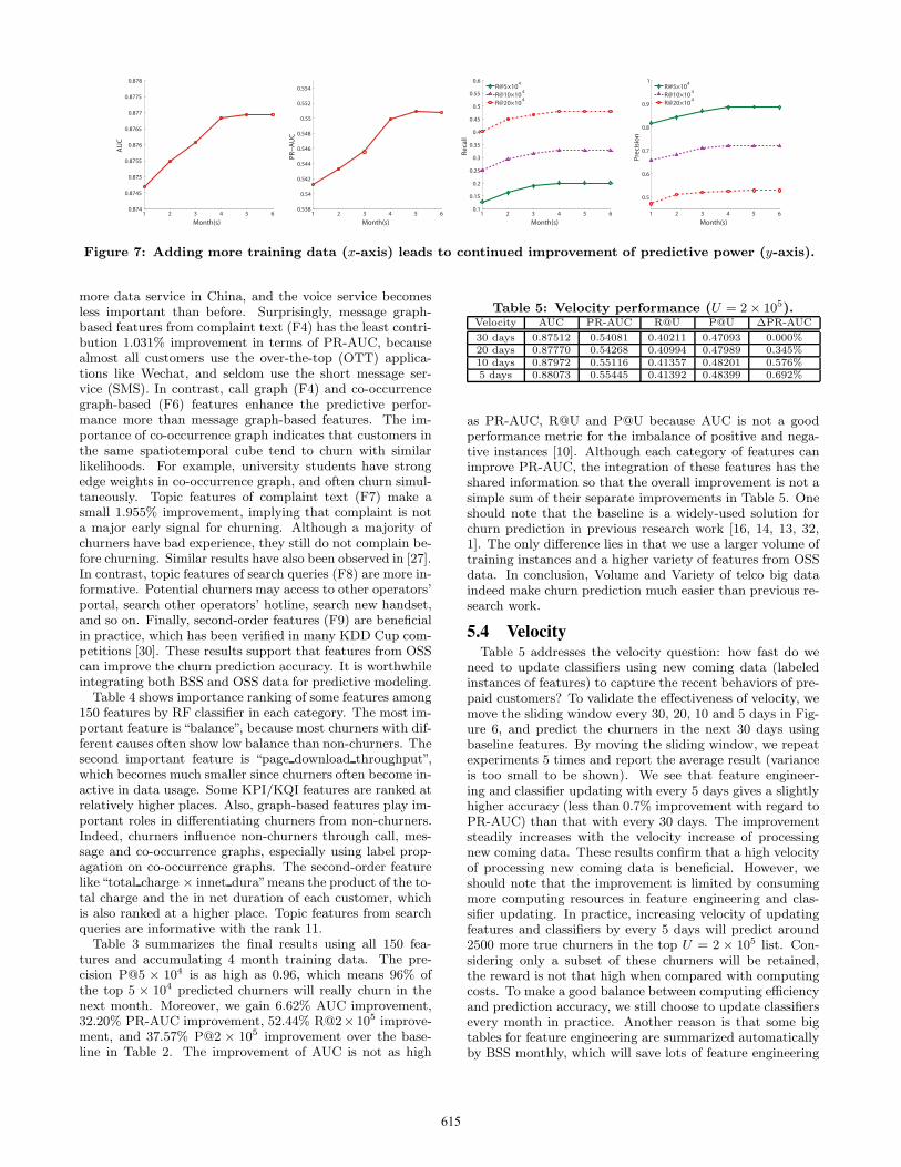
5.2 VolumeFigure 7 examines the question: when using baseline fea-

tures in Section 4.1, do we indeed see increasing predictiveperformance as the training dataset continues to grow tomassive size? This experiment aims to predict the poten-tial churners in Month 7 in Table 1 by accumulating thelabeled instances of feature vectors from Month 6 to Month1. Such a experiment repeats 3 times to predict churnersin Months 7, 8 and 9 by the sliding window in Figure 6,and the average results are reported (variance is too smallto be shown). As Figure 7 shows (x-axis denotes volumeof training data measured by the number of months and yis the predictive performance metrics AUC, PR-AUC, R@Uand P@U), the performance keeps improving even when weadd more than 4 times larger training data. We show re-sults on U = {5× 104, 1× 105, 2 × 105}, which denotes thenumber of predicted churners with top largest likelihoods.As far as R@5 × 104 is concerned, the larger training dataachieves around 15% improvement, confirming that the Vol-ume of big telco data indeed matters. This result suggeststhat telco operators need to store at least 4 months’ datafor a better churn prediction performance.

One should note, however, that the AUC, PR-AUC, R@Uand P@U curves do seem to show some diminishing returnsto scale. This is typical for the relationship between theamount of data and predictive performance, especially forlinear models like logistic regression [36]. The marginal in-crease in generalization accuracy decreases with more train-ing data for two reasons. First, the classifier may be toosimple to capture the statistical variance of larger dataset.There is a maximum possible predictive performance due tothe fact that accuracy can never be better than perfect. Sec-ond, more importantly, accumulating more earlier trainingdata in past months may be not helpful in predicting po-tential churners in recent months. For example, the churnerbehaviors in Month 1 may be quite different from those inMonth 7. Adding training data in Month 1 can provide lit-tle information to predict churners in Month 7. This followsthe temporal first-order Markov property: the present statedepends only on the most closest previous state.

5.3 VarietyThe experiments reported above confirm that Volume (the

number of training instances) can improve the predictive

Table 3: The overall predictive performance.Top U Recall Precision AUC PR-AUC

50000 0.22775 0.95928

0.93261 0.71553

100000 0.41198 0.86764150000 0.53930 0.75719200000 0.62884 0.66218250000 0.69362 0.58431300000 0.74550 0.52334350000 0.78498 0.47234400000 0.81621 0.42974

Table 4: Importance ranking of some features.Rank Features Category Importance

1 balance F1 0.1633362 page download throughput F3 0.1597723 localbase call dur F1 0.0839486 page response delay F3 0.0519109 voice quality F2 0.03673211 search txt topic F8 0.01501417 innet dura× total charge F9 0.00886741 labelpropaagtion cooccurrence F6 0.00350754 pagerank voice F4 0.00070368 pagerank cooccurence F5 0.000518

modeling accuracy. An alternative perspective on increasingdata size is to consider a fixed number of training instancesand increase the number of different possible features (Vari-ety) that are collected, stored or utilized for each instance.This Variety perspective of big data motivates us to exploreextensively OSS features plus BSS features. We believe thatpredictive modeling may benefit from a large variety of fea-tures if most of the features provide a small but non-zeroamount of additional information about target prediction.To this end, we add separately the following categories offeatures to the baseline features (F1 for BSS features) oneby one in Table 2: F2 for CS features, F3 for PS features, F4for Call graph-based features, F5 for Message graph-basedfeatures, F6 for Co-occurence graph-based features, F7 forTopic features (complaints), F8 for Topic features (searchqueries), F9 for Second-order features. There are 150 fea-tures (F1: 70, F2: 9, F3: 25, F4: 2, F5: 2, F6: 2, F7: 10, F8:10, F9: 20), and detailed descriptions on these features canbe found in Section 4.1. On our dataset in Table 1, we re-peat this experiment 7 times to predict churners in Months3 ∼ 9, using one month labeled features for training andpredict the potential churners in the next month as shownin Figure 6. The average results are reported (variance istoo small to be shown).

Table 2 summarizes the contribution of each category offeatures to the baseline features. CS and PS features (F2 andF3) contribute significantly 12.483% and 14.871% improve-ments on PR-AUC, respectively. This result is promisingbecause churners are quite related with KPI/KQI featuresfrom both voice and data services. We can use a customer-centric network optimization solution to improve KPI/KQIexperiences of potential churners. PS features are more ef-fective than CS features because customers use more and

614

1 2 3 4 5 60.874

0.8745

0.875

0.8755

0.876

0.8765

0.877

0.8775

0.878

Month(s)

AU

C

1 2 3 4 5 60.538

0.54

0.542

0.544

0.546

0.548

0.55

0.552

0.554

Month(s)

PR−

AU

C

1 2 3 4 5 60.1

0.15

0.2

0.25

0.3

0.35

0.4

0.45

0.5

0.55

0.6

Month(s)

Reca

ll

1 2 3 4 5 6

0.5

0.6

0.7

0.8

0.9

1

Month(s)

Prec

isio

n

R@5×10 R@10×10R@20×10

4

4

4

R@5×10 R@10×10R@20×10

4

4

4

Figure 7: Adding more training data (x-axis) leads to continued improvement of predictive power (y-axis).

more data service in China, and the voice service becomesless important than before. Surprisingly, message graph-based features from complaint text (F4) has the least contri-bution 1.031% improvement in terms of PR-AUC, becausealmost all customers use the over-the-top (OTT) applica-tions like Wechat, and seldom use the short message ser-vice (SMS). In contrast, call graph (F4) and co-occurrencegraph-based (F6) features enhance the predictive perfor-mance more than message graph-based features. The im-portance of co-occurrence graph indicates that customers inthe same spatiotemporal cube tend to churn with similarlikelihoods. For example, university students have strongedge weights in co-occurrence graph, and often churn simul-taneously. Topic features of complaint text (F7) make asmall 1.955% improvement, implying that complaint is nota major early signal for churning. Although a majority ofchurners have bad experience, they still do not complain be-fore churning. Similar results have also been observed in [27].In contrast, topic features of search queries (F8) are more in-formative. Potential churners may access to other operators’portal, search other operators’ hotline, search new handset,and so on. Finally, second-order features (F9) are beneficialin practice, which has been verified in many KDD Cup com-petitions [30]. These results support that features from OSScan improve the churn prediction accuracy. It is worthwhileintegrating both BSS and OSS data for predictive modeling.

Table 4 shows importance ranking of some features among150 features by RF classifier in each category. The most im-portant feature is “balance”, because most churners with dif-ferent causes often show low balance than non-churners. Thesecond important feature is “page download throughput”,which becomes much smaller since churners often become in-active in data usage. Some KPI/KQI features are ranked atrelatively higher places. Also, graph-based features play im-portant roles in differentiating churners from non-churners.Indeed, churners influence non-churners through call, mes-sage and co-occurrence graphs, especially using label prop-agation on co-occurrence graphs. The second-order featurelike“total charge × innet dura”means the product of the to-tal charge and the in net duration of each customer, whichis also ranked at a higher place. Topic features from searchqueries are informative with the rank 11.

Table 3 summarizes the final results using all 150 fea-tures and accumulating 4 month training data. The pre-cision P@5 × 104 is as high as 0.96, which means 96% ofthe top 5 × 104 predicted churners will really churn in thenext month. Moreover, we gain 6.62% AUC improvement,32.20% PR-AUC improvement, 52.44% R@2× 105 improve-ment, and 37.57% P@2 × 105 improvement over the base-line in Table 2. The improvement of AUC is not as high

Table 5: Velocity performance (U = 2× 105).Velocity AUC PR-AUC R@U P@U ΔPR-AUC

30 days 0.87512 0.54081 0.40211 0.47093 0.000%20 days 0.87770 0.54268 0.40994 0.47989 0.345%10 days 0.87972 0.55116 0.41357 0.48201 0.576%5 days 0.88073 0.55445 0.41392 0.48399 0.692%

as PR-AUC, R@U and P@U because AUC is not a goodperformance metric for the imbalance of positive and nega-tive instances [10]. Although each category of features canimprove PR-AUC, the integration of these features has theshared information so that the overall improvement is not asimple sum of their separate improvements in Table 5. Oneshould note that the baseline is a widely-used solution forchurn prediction in previous research work [16, 14, 13, 32,1]. The only difference lies in that we use a larger volume oftraining instances and a higher variety of features from OSSdata. In conclusion, Volume and Variety of telco big dataindeed make churn prediction much easier than previous re-search work.

5.4 VelocityTable 5 addresses the velocity question: how fast do we

need to update classifiers using new coming data (labeledinstances of features) to capture the recent behaviors of pre-paid customers? To validate the effectiveness of velocity, wemove the sliding window every 30, 20, 10 and 5 days in Fig-ure 6, and predict the churners in the next 30 days usingbaseline features. By moving the sliding window, we repeatexperiments 5 times and report the average result (varianceis too small to be shown). We see that feature engineer-ing and classifier updating with every 5 days gives a slightlyhigher accuracy (less than 0.7% improvement with regard toPR-AUC) than that with every 30 days. The improvementsteadily increases with the velocity increase of processingnew coming data. These results confirm that a high velocityof processing new coming data is beneficial. However, weshould note that the improvement is limited by consumingmore computing resources in feature engineering and clas-sifier updating. In practice, increasing velocity of updatingfeatures and classifiers by every 5 days will predict around2500 more true churners in the top U = 2 × 105 list. Con-sidering only a subset of these churners will be retained,the reward is not that high when compared with computingcosts. To make a good balance between computing efficiencyand prediction accuracy, we still choose to update classifiersevery month in practice. Another reason is that some bigtables for feature engineering are summarized automaticallyby BSS monthly, which will save lots of feature engineering

615

Table 6: Business value of churn prediction.

MonthGroup A

Top 5 × 104 Top 5 × 104 ∼ 1 × 105

Total Recharge Rate Total Recharge Rate8 7994 134 1.68% 8032 808 10.06%9 8024 84 1.04% 8050 798 9.91%

MonthGroup B

Top 5 × 104 Top 5 × 104 ∼ 1 × 105

Total Recharge Rate Total Recharge Rate8 7972 1474 18.49% 8026 2280 28.41%9 7988 2458 30.77% 8042 3194 39.72%

costs since we do not need to re-generate these big tablesmanually by every 5 days. So, Table 3 summarizes the finalpredictive performance of our deployed churn prediction sys-tem (Volume = 4 months, Variety = 140 features, Velocity= 1 month).

5.5 ValueThe business value is a major concern of the deployed

churn prediction and retention system. Every month, thesystem provides a list of top U = 1× 105 potential churnersranking by classification likelihoods (4), which covers around40% true churners as shown in Table 3. We select a subsetof potential churners4 (some from top 5 × 104 and othersfrom top 5×104 ∼ 1×105) for the following prepaid mobilerecharge offers: 1) Get 100 cashback on recharge of 100, 2)Get 50 cashback on recharge of 100, 3) Get 500MB flux onrecharge of 50, and 4) Get 200-minute voice call on rechargeof 50, when they enter the recharge period. In the A/B test,it is desirable to see a very low recharge rate of the predictedpotential churners without recharge offers (Group A), anda relatively higher recharge rate of potential churners withrecharge offers (Group B). We carry out retention campaignsin two consecutive months 8 and 9. In Month 8, we do nottrain retention classifiers in Figure 6 to match churners withrecharge offers, but send offers by short message service tochurners according to domain knowledge guided by operatorexperts. In Month 9, we use the campaign results as labels(customers who accept different offers are defined as differentclass labels in Subsection 4.3) to build a retention classifier,matching proper offers with churners automatically. In thisway, we can gradually improve the retention efficiency toretain more potential churners.

Table 6 shows the recharge rates of A/B test in Months8 and 9. In group A, the recharge rate is very low in bothMonths 8 and 9. In top 5 × 104 predicted churners, therecharge rate is less than 2%, which means 98% predictedchurners in recharge period will not recharge within 15 days.In top 5 × 104 ∼ 1 × 105 predicted churners, the rechargerate is around 10%. All these results confirm that the highaccuracy of the churn prediction system. In Month 8, ran-domly assigning recharge offers in Group B can significantlyenhance the recharge rate, e.g., from 1.68% to 18.48% andfrom 10.06% to 28.41%, when compared with Group A. Fur-thermore, in Month 9, after matching recharge offers withchurners in Group B, we see a further significant increase ofrecharge rate, e.g., from 1.04% to 30.77% and from 9.91% to39.72%, when compared with Group A. Indeed, the strategyof matching offers with churners in Month 9 can retain morepotential churners, which leads to around 50% more profit

4This is a small-scale test due to the limitation of retentionresources at that time.

Table 7: Comparison of methods for data imbalance.Methods AUC PR-AUC R@U P@U

Not Balanced 0.83712 0.49092 0.38969 0.43239Up Sampling 0.84140 0.51882 0.39180 0.44187

Down Sampling 0.84791 0.51967 0.39757 0.45101Weighted Instance 0.87468 0.54123 0.41251 0.48133

than Month 8. This provides one of the clearest illustra-tion that the integration of churn prediction and retentionsystem is indeed more valuable. From this perspective, ourprediction target changes to those potential churners with ahigher likelihood to be retained by a specific retention offer.

5.6 Early SignalsTelco operators wish to predict churners as early as pos-

sible to provide proper retention strategies in a timely andprecise manner. In this setting, we change the sliding win-dow in Figure 6. We use labels in Month N +2 and featuresin Month N − 1 to train the classifier, and use features inMonth N and the classifier to predict the potential churnersin Month N +3. This setting can predict churners 3 monthsearlier. Similarly, we can change the experimental settingto predict churners from 1 ∼ 4 months earlier. Using base-line features, we show the predictive performance of earlierfeatures in Figure 8. Obviously, the earlier features pro-vide the worse predictive performance. The accuracy signif-icantly decreases with the increase of time interval betweenthe observed features and the predicted labels in Figure 6.For example, the PR-AUC drops around 20% using featuresfrom 1 month to 2 month earlier for prediction. The re-sults imply that the prepaid customers often churn abruptlywithout providing enough early signals. Most churners showtheir abnormal behaviors just before a month. These obser-vations are consistent with Figure 7, where adding moreearlier instances of features provides little additional infor-mation to improve predictive performance.

5.7 Data ImbalanceData imbalance has long been discussed in building clas-

sifiers [6, 15]. There are four widely-used methods to han-dle data imbalance: 1) Not Balanced, 2) Up Sampling, 3)Down Sampling and 4) Weighted Instance. The first methoddirectly train classifier using imbalanced churner and non-churner instances. The second method randomly copies thechurner instances to the same number of non-churner in-stances. The third method randomly samples a subset ofnon-churner instances to the same number of churner in-stances. The fourth method assigns a proportion weight toeach instance, where higher weights are assigned to churn-ers and lower weights to non-churners. We use baseline fea-tures to evaluate different methods for data imbalance. Ta-ble 7 shows the average predictive performance using differ-ent methods (variance is too small to be shown). Clearly, theWeighted Instance method outperforms other methods, hav-ing around 10% improvement over the Not Balanced methodin terms of PR-AUC. So, we advocate the Weighted Instancemethod to handle data imbalance in practice.

5.8 ClassifiersWe compare some widely used classifiers in data min-

ing: RF, LIBFM, LIBLINEAR (L2-regularized logistic re-gression) and GBDT. Some classifiers have won KDD CUP

616

1 2 3 40.65

0.7

0.75

0.8

0.85

0.9

Month(s)

AU

C

1 2 3 4

0.1

0.2

0.3

0.4

0.5

0.6

Month(s)

PR−

AU

C

1 2 3 40.1

0.2

0.3

0.4

0.5

0.6

Month(s)

Reca

ll

1 2 3 40

0.2

0.4

0.6

0.8

1

Month(s)

Prec

isio

n

R@5×10R@10×10R@20×10

4

4

4

R@5×10R@10×10R@20×10

4

4

4

Figure 8: The earlier features produce worse predictive performance.

AUC PR−AUC0.3

0.4

0.5

0.6

0.7

0.8

0.9

1.0

RFLIBFMGBRTLIBLINEAR

Figure 9: Comparison of different classifiers.

champions based on complicated feature engineering tech-niques [13, 36, 30]. RF and GBDT fix 500 decision treeswith default parameter settings. For example, the learn-ing rate of GBRT, LIBFM and LIBLINEAR is fixed as 0.1.LIBFM and LIBLINEAR use discrete binary features bypreprocessing the original continuous feature values, becauselinear models are more suitable for sparse binary features.Using the same baseline features, we find that RF performsslightly better (less than 3%) than other classifiers in Fig-ure 9 in terms of AUC and PR-AUC. The results are con-sistent with several previous research works advocating RFclassifier for churn prediction [21, 7, 27]. Nevertheless, theclassifiers are not as important as features. Given a vari-ety of features, most scalable classifiers can achieve almostthe same accuracy. The result indicates that adding a goodfeature may enhance the predictive modeling more signifi-cantly than changing to a better classifier, which have im-portant implications for telco operators faced with competi-tion. Telco operators dealing with larger data assets, moreimportant than prediction techniques, potentially can ob-tain substantial competitive advantages over telco operatorswithout access to so much data.

6. CONCLUSIONSThis paper re-explores an old but classic research topic in

telco industry—churn prediction—from the 3V’s perspec-tives of big data. Releasing the power of telco big datacan indeed enhance the performance of predictive analytics.Extensive results demonstrate that Variety plays a more im-portant role in telco churn prediction, when compared withVolume and Velocity. This suggests that telco operators

should consider gathering, storing, and utilizing big OSSdata to enrich Variety, which occupy more than 90% sizeof the entire telco data assets. Integration of BSS and OSSdata leads to a better automatic churn prediction and re-tention system with a big business value. Extension workincludes inferring root causes of churners for actionable andsuitable retention strategies.

Previous churn prediction research is based only on BSSdata such as call/billing records, purchase history, paymentrecords, and CDRs, because it is much easier to acquire BSSdata. In contrast, OSS data are much less consistent andmuch harder to acquire, because telco operators need do-main knowledge from OSS/hardware vendors’ systems theyhave. In OSS, the data quality and format will vary greatlyamong telco operators since each has their own software andhardware vendors. The cost of acquiring OSS data is oftenhigh, because of the large volume of data storage as well aslicense fees charged by OSS/hardware vendors. Therefore,the key challenge of the telco big data platform is the OSSdata cleaning and integration layer as shown in Figure 2.However, OSS data do have big business value for accuratelocation information, mobile search queries and customer-centric network quality measurements. If OSS data analysisis done with appropriate technique, it can reward for thetelco operators, some of which have claimed that they havebeen generating millions of revenue by selling OSS data anal-ysis results. In this paper, our results on churn predictionalso confirm that OSS data have cost-cutting and revenue-increasing benefits when combined with BSS data.

AcknowledgmentsThis work was supported by National Grant FundamentalResearch (973 Program) of China under Grant 2014CB340304,NSFC (Grant No. 61373092 and 61033013), Hong KongRGC project 620812, and Natural Science Foundation of theJiangsu Higher Education Institutions of China (Grant No.12KJA520004). This work was partially supported by Col-laborative Innovation Center of Novel Software Technologyand Industrialization.

7. REFERENCES[1] A. M. Almana, M. S. Aksoy, and R. Alzahrani. A survey on

data mining techniques in customer churn analysis fortelecom industry. Journal of Engineering Research andApplications, 4(5):165–171, 2014.

[2] W. Au, K. Chan, and X. Yao. A novel evolutionary datamining algorithm with applications to churn prediction.IEEE Trans. on Evolutionary Computation, 7(6):532–545,2003.

617

[3] K. binti Oseman, S. binti Mohd Shukor, N. A. Haris, andF. bin Abu Bakar. Data mining in churn analysis model fortelecommunication industry. Journal of Statistical Modelingand Analytics, 1:19–27, 2010.

[4] D. M. Blei, A. Y. Ng, and M. I. Jordan. Latent Dirichletallocation. J. Mach. Learn. Res., 3:993–1022, 2003.

[5] L. Breiman. Random forests. Machine learning, 45(1):5–32,2001.

[6] J. Burez and D. Van den Poel. Handling class imbalance incustomer churn prediction. Expert Systems withApplications, 36(3):4626–4636, 2009.

[7] K. Coussement and D. Van den Poel. Churn prediction insubscription services: An application of support vectormachines while comparing two parameter-selectiontechniques. Expert systems with applications,34(1):313–327, 2008.

[8] K. Dasgupta, R. Singh, B. Viswanathan, D. Chakraborty,S. Mukherjea, A. A. Nanavati, and A. Joshi. Social ties andtheir relevance to churn in mobile telecom networks. InEDBT, pages 668–677, 2008.

[9] P. Datta, B. Masand, D. Mani, and B. Li. Automatedcellular modeling and prediction on a large scale. ArtificialIntelligence Review, 14(6):485–502, 2000.

[10] J. Davis and M. Goadrich. The relationship betweenPrecision-Recall and ROC curves. In ICML, pages 233–240,2006.

[11] E. J. de Fortuny, D. Martens, and F. Provost. Predictivemodeling with big data: Is bigger really better? Big Data,1(4):215–226, 2013.

[12] R.-E. Fan, K.-W. Chang, C.-J. Hsieh, X.-R. Wang, andC.-J. Lin. LIBLINEAR: A library for large linearclassification. Journal of Machine Learning Research,9:1871–1874, 2008.

[13] I. Guyon, V. Lemaire, M. Boulle, G. Dror, and D. Vogel.Analysis of the KDD Cup 2009: Fast scoring on a largeorange customer database. 7:1–22, 2009.

[14] J. Hadden, A. Tiwari, R. Roy, and D. Ruta. Computerassisted customer churn management: State-of-the-art andfuture trends. Computers & Operations Research,34(10):2902–2917, 2007.

[15] H. He and E. Garcia. Learning from imbalanced data.IEEE Trans. on Knowledge and Data Engineering,21(9):1263–1284, 2009.

[16] S. Hung, D. Yen, and H. Wang. Applying data mining totelecom churn management. Expert Systems withApplications, 31(3):4515–524, 2006.

[17] S. Jiang, G. A. Fiore, Y. Yang, J. Ferreira Jr, E. Frazzoli,and M. C. Gonzalez. A review of urban computing formobile phone traces: current methods, challenges andopportunities. In KDD Workshop on Urban Computing,pages 2–9, 2013.

[18] S. Jinbo, L. Xiu, and L. Wenhuang. The application ofAdaBoost in customer churn prediction. In InternationalConference on Service Systems and Service Management,pages 1–6, 2007.

[19] M. Karnstedt, M. Rowe, J. Chan, H. Alani, and C. Hayes.The effect of user features on churn in social networks. InACM Web Science Conference, pages 14–17, 2011.

[20] N. Kim, K.-H. Jung, Y. S. Kim, and J. Lee. Uniformlysubsampled ensemble (use) for churn management: Theoryand implementation. Expert Systems with Applications,39(15):11839–11845, 2012.

[21] A. Lemmens and C. Croux. Bagging and boostingclassification trees to predict churn. Journal of MarketingResearch, 43(2):276–286, 2006.

[22] E. Lima, C. Mues, and B. Baesens. Domain knowledgeintegration in data mining using decision tables: Casestudies in churn prediction. Journal of the OperationalResearch Society, 60(8):1096–1106, 2009.

[23] N. Lu, H. Lin, J. Lu, and G. Zhang. A customer churn

prediction model in telecom industry using boosting. IEEETrans. on Industrial Informatics, 10(2):1659–1665, 2014.

[24] S. Neslin, S. Gupta, W. Kamakura, J. Lu, and C. Mason.Detection defection: Measuring and understanding thepredictive accuracy of customer churn models. Journal ofMarketing Research, 43(2):204–211, 2006.

[25] M. Owczarczuk. Churn models for prepaid customers in thecellular telecommunication industry using large data marts.Expert Systems with Applications, 37(6):4710–4712, 2010.

[26] L. Page, S. Brin, R. Motwani, and T. Winograd. Thepagerank citation ranking: Bringing order to the web. 1999.

[27] C. Phua, H. Cao, J. B. Gomes, and M. N. Nguyen.Predicting near-future churners and win-backs in thetelecommunications industry. arXiv preprintarXiv:1210.6891, 2012.

[28] Pushpa and S. Dr.G. An efficient method of building thetelecom social network for churn prediction. InternationalJournal of Data Mining & Knowledge ManagementProcess, 2:31–39, 2012.

[29] D. Radosavljevik, P. van der Putten, and K. K. Larsen. Theimpact of experimental setup in prepaid churn predictionfor mobile telecommunications: What to predict, for whomand does the customer experience matter? Transactions onMachine Learning and Data Mining, 3(2):80–99, 2010.

[30] S. Rendle. Scaling factorization machines to relational data.In PVLDB, volume 6, pages 337–348, 2013.

[31] K. Shvachko, H. Kuang, S. Radia, and R. Chansler. Thehadoop distributed file system. In IEEE Symposium onMass Storage Systems and Technologies (MSST), pages1–10, 2010.

[32] W. Verbeke, K. Dejaeger, D. Martens, J. Hur, andB. Baesens. New insights into churn prediction in thetelecommunication sector: A profit driven data miningapproach. European Journal of Operational Research,218(1):211–229, 2012.

[33] W. Verbeke, D. Martens, C. Mues, and B. Baesens.Building comprehensible customer churn prediction modelswith advanced rule induction techniques. Expert systemswith applications, 38:2354–2364, 2011.

[34] C.-P. Wei and I. Chiu. Turning telecommunications calldetails to churn prediction: a data mining approach. Expertsystems with applications, 23(2):103–112, 2002.

[35] E. Xevelonakis. Developing retention strategies based oncustomer profitability in telecommunications: An empiricalstudy. Journal of Database Marketing & Customer StrategyManagement, 12:226–242, 2005.

[36] H.-F. Yu, H.-Y. Lo, H.-P. Hsieh, J.-K. Lou, T. G.McKenzie, J.-W. Chou, P.-H. Chung, C.-H. Ho, C.-F.Chang, Y.-H. Wei, et al. Feature engineering and classifierensemble for kdd cup 2010. In JMLR W & CP, pages 1–16,2010.

[37] M. Zaharia, M. Chowdhury, M. J. Franklin, S. Shenker, andI. Stoica. Spark: Cluster computing with working sets. InHotCloud, 2010.

[38] J. Zeng. A topic modeling toolbox using belief propagation.J. Mach. Learn. Res., 13:2233–2236, 2012.

[39] J. Zeng, W. K. Cheung, and J. Liu. Learning topic modelsby belief propagation. IEEE Trans. Pattern Anal. Mach.Intell., 35(5):1121–1134, 2013.

[40] X. Zhu and Z. Ghahramani. Learning from labeled andunlabeled data with label propagation. Technical report,Technical Report CMU-CALD-02-107, Carnegie MellonUniversity, 2002.

618