telematics chapter 6: network layer - freie universität · · 2012-09-03telematics chapter 6:...

Telematics

Chapter 6: Network Layer

Univ.-Prof. Dr.-Ing. Jochen H. Schiller

Computer Systems and Telematics (CST)

Institute of Computer Science

Freie Universität Berlin

http://cst.mi.fu-berlin.de

Data Link Layer

Presentation Layer

Session Layer

Physical Layer

Network Layer

Transport Layer

Application Layer

Data Link Layer

Presentation Layer

Session Layer

Physical Layer

Network Layer

Transport Layer

Application Layer

Data Link Layer

Physical Layer

Network Layer

User watching video clip

Server with video clips

http://cst.mi.fu-berlin.de/



6.2

Contents

● Design Issues

● The Internet

● Internet Protocol (IP)

● Internet Protocol Version 6 (IPv6)

● Network Address Translation

(NAT)

● Auxiliary Protocols

● Address Resolution Protocols (ARP)

● Reverse ARP (RARP)

● Dynamic Host Configuration

Protocol (DHCP)

● Internet Control Message Protocol (ICMP)

● Routing

● Shortest Path Routing

● Distance Vector Routing

● Routing Information Protocol

(RIP)

● Link State Routing

● Hierarchical Routing

● Open Shortest Path First (OSPF)

● Border Gateway Protocol (BGP)

● Internet Group Management

Protocol (IGMP)

Univ.-Prof. Dr.-Ing. Jochen H. Schiller ▪ cst.mi.fu-berlin.de ▪ Telematics ▪ Chapter 6: Network Layer

6.3

Connection principles

Design Issues


6.4

Layer 3

● Layer 1/2 are responsible only for

the transmission of data between

adjacent computers.

● Layer 3: Network Layer

● Boundary between network

carrier and customer

● Control of global traffic

● Coupling of sub-networks

● Global addressing

● Routing of data packets

● Initiation, management and

termination of connections through the whole network

● Global flow control

Data Link Layer

Presentation Layer

Session Layer

Physical Layer

Network Layer

Transport Layer

Application Layer

OSI Reference Model


6.5

Layers in the Network

Physical Layer

Data Link Layer

Network Layer

Transport Layer

Session Layer

Presentation Layer

Application Layer

Application Process

Physical Layer

Data Link Layer

Network Layer

Transport Layer

Session Layer

Presentation Layer

Application Layer

Application Process

Physical Layer

Data Link Layer

Network Layer

Physical Layer

Data Link Layer

Network Layer

Host A Host B Router A Router B

Routers in the network receive frames from layer 2, extract the layer 3 content (packet) and decide based on the global address to which outgoing connection (port) the packet has to be passed on. Accordingly the packet becomes payload of a new frame and is sent.


6.6

Layers in the Network


Data Link Layer Physical Layer

Network Layer


Network Layer


Network Layer

One protocol on the network layer

Technology 1 Ethernet MTU 1500 bytes

Technology 2 Tokenring, DSL MTU 512 bytes

6.7

Two Fundamental Philosophies

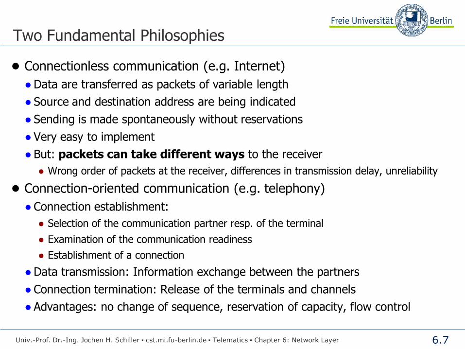
● Connectionless communication (e.g. Internet)

● Data are transferred as packets of variable length

● Source and destination address are being indicated

● Sending is made spontaneously without reservations

● Very easy to implement

● But: packets can take different ways to the receiver

● Wrong order of packets at the receiver, differences in transmission delay, unreliability

● Connection-oriented communication (e.g. telephony)

● Connection establishment:

● Selection of the communication partner resp. of the terminal

● Examination of the communication readiness

● Establishment of a connection

● Data transmission: Information exchange between the partners

● Connection termination: Release of the terminals and channels

● Advantages: no change of sequence, reservation of capacity, flow control


6.8

Connectionless Communication

Computer A

Computer C

Computer B

Packet Switching

Message is divided into packets

Access is always possible, small susceptibility to faults

Alternative paths for the packets

Additional effort in the nodes: Store-and-Forward network

1 3 2


6.9

Connection-Oriented Communication

Computer A

Computer C

Computer B

Circuit Switching

Simple communication method

Defined routes between the participants

Switching nodes connect the lines

Exclusive use of the line (telephone) or virtual connection:

Establishment of a connection over a (possibly even packet switching) network

virtual connection

1 2 3


6.10

Routing principles

Design Issues


6.11

Routing

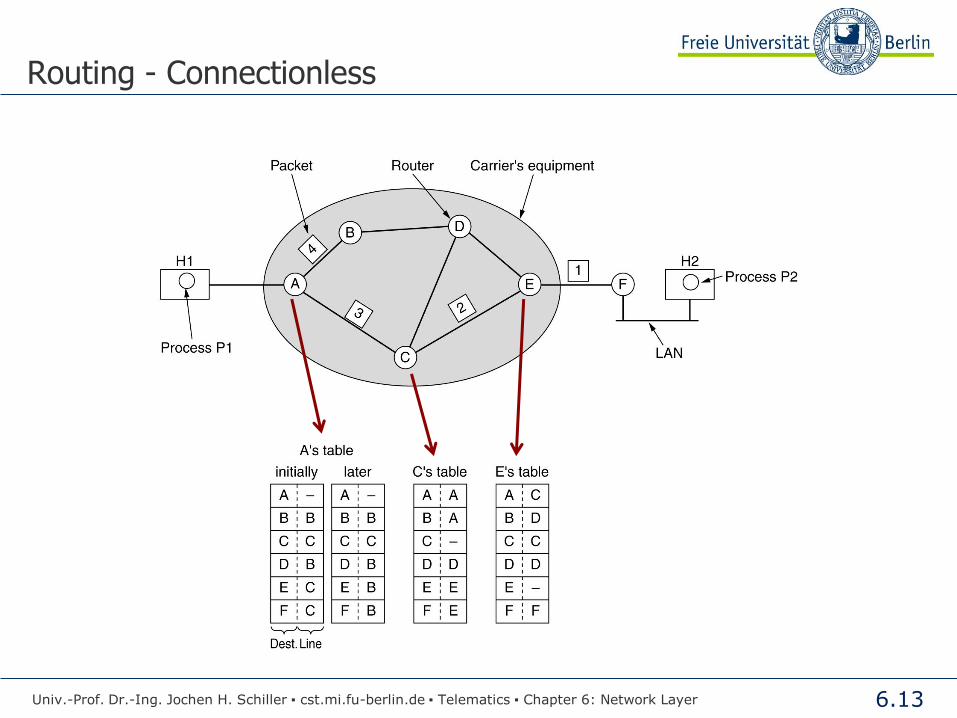
● Most important functionality on Layer 3 is addressing and routing.

● Each computer has to be assigned a worldwide unique address

● Every router manages a table (Routing Table) which indicates, which outgoing connection has to be selected for a certain destination.

● The routing tables can be determined statically; however it is better to adapt them dynamically to the current network status.

● With connectionless communication, the routing must be done for each packet separately. The routing decision can vary from packet to packet.

● With virtual connections, routing is done only once (connection establishment, see ATM), but the routing tables are more extensive

To destination By connection

A L2

B L1

C L3

D L2


L1

L2

L3

L4

6.12

Routing

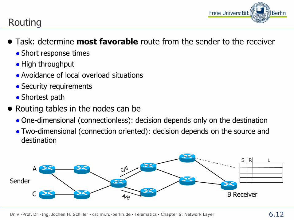
● Task: determine most favorable route from the sender to the receiver

● Short response times

● High throughput

● Avoidance of local overload situations

● Security requirements

● Shortest path

● Routing tables in the nodes can be

● One-dimensional (connectionless): decision depends only on the destination

● Two-dimensional (connection oriented): decision depends on the source and

destination


C

Sender

B Receiver

L S R

A

6.13

Routing - Connectionless


6.14

Routing - Connection-oriented

Source computer, connection ID Next computer, connection ID

Related terms Virtual circuit Label switching


6.15

Routing – Comparison

Issue Connectionless Datagram Subnet

Connection-oriented Virtual-circuit Subnet

Circuit setup Not needed Required

Addressing Each packet contains the full source and destination address

Each packet contains a short VC ID

State information Routers do not hold state information about connections

Each VC requires router table space per connection

Routing Each packet is routed independently

Route chosen when VC is set up; all packets follow it

Effect of router failures

None, except for packets lost during the crash

All VCs that passed through the failed router are terminated

Quality of service Difficult Easy if enough resources can be allocated in advance for each VC

Congestion control Difficult Easy if enough resources can be allocated in advance for each VC


6.16

X X’

A B C

A’ B’ C’

● High traffic amount between A and A’, B and B’, C and C’

● In order to optimize the total data flow, no traffic may occur between X and X’

● X and X’ would see this totally different!

fairness criteria!

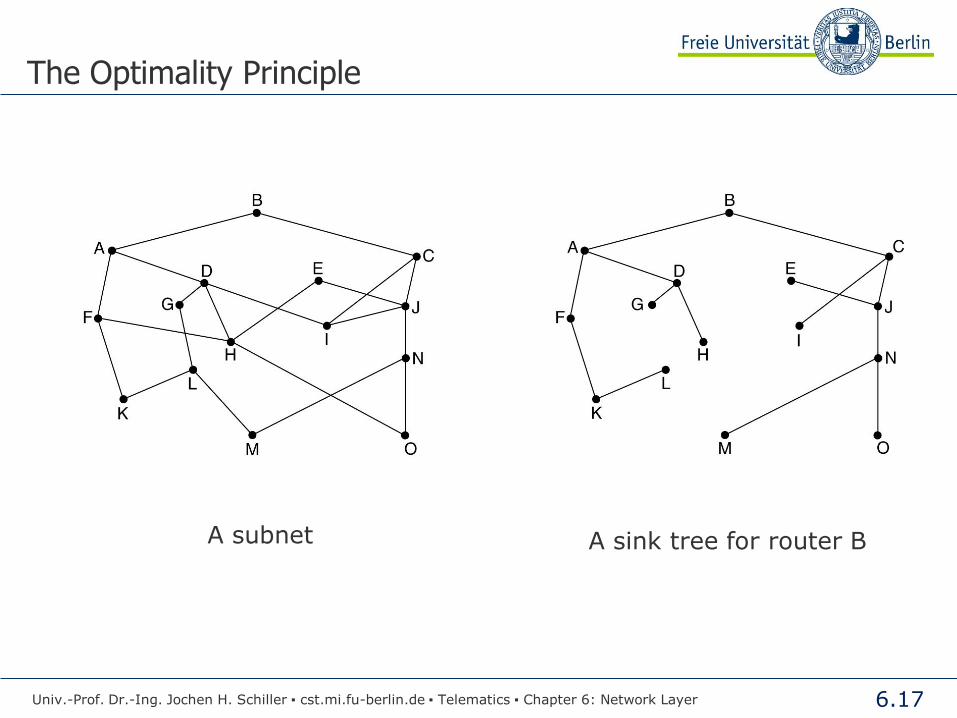
“Optimal” Routing

● “Optimal” route decision is in principle not possible, because

● no complete information about the network is present within the individual nodes

● a routing decision effects the network for a certain period

● conflicts between fairness and optimum can arise


6.17

The Optimality Principle


A subnet A sink tree for router B

6.18

Maximum capacity

of the network

Perfect

Desirable

Overloaded

Sent packets

Delivere

d p

ackets

With excessive traffic, the performance of the network decreases rapidly

Solution: “smoothing” of the traffic amount, i.e., adjustment of the data rate.

Traffic Shaping

Parameters for detecting overload:

● Average length of the router queues

● Portion of the discarded packets in a router

● Number of packets in a router

● Number of packet retransmissions

● Average transmission delay from the sender to the receiver

● Standard deviation of the transmission delay

Congestion Control


6.19

Internet


6.20

On the Way to Today's Internet

● Goal:

● Interconnection of computers and networks using uniform protocols

● A particularly important initiative was initiated by the ARPA

(Advanced Research Project Agency, with military interests)

● The participation of the military was the only sensible way to implement such an

ambitious and extremely expensive project

● The OSI specification was still in developing phase

● Result: ARPANET (predecessor of today's Internet)


6.21

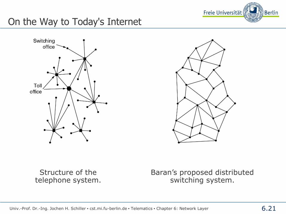
On the Way to Today's Internet


Structure of the telephone system.

Baran’s proposed distributed switching system.

6.22

Design objective for ARPANET

● The operability of the network should remain intact even after a large disaster, e.g., a nuclear war, thus high connectivity and connectionless transmission

● Network computers and host computers are separated

ARPA

Advanced Research

Projects Agency

ARPANET

1969

ARPANET


Subnet

6.23

A subnet consists of:

● Interface Message Processors (IMPs), which are connected by leased transmission circuits

● High connectivity (in order to guarantee the demanded reliability)

IMP

Subnet

Source IMP to destination IMP protocol

Host-host Protocol

Host-IMP Protocol

A node consists of

● an IMP

● a host

Several protocols for the communication between IMP-IMP, host-IMP,…

ARPANET


6.24

DEK PDP-10

XDS 940

XDS 1-7

Stanford Research

Institute (SRI)

University

of Utah

University of California

Los Angeles (UCLA)

University of California Santa Barbara (UCSB)

ARPANET (December 1969)

IMP

IMP

IBM 360/75

IMP

IMP California

The Beginning of ARPANET


6.25

SRI

UCSB

UCLA

Utah

WITH

Harvard

Illinois

USC

SRI Utah Illinois WITH

USC UCLA

UCSB

Stanford

Harvard Aberdeen

CMU

ARPANET in April 1972 ARPANET in September 1972

Very fast evolution of the ARPANET within shortest time:

Evolution by ARPANET


6.26

Interworking

● Problem: Interworking!

● Simultaneously to the ARPANET other (smaller) networks were developed

● All the LANs, MANs, WANs, ...

● had different protocols, media, ...

● could not be interconnected at first and were not be able to communicate with each other

● Therefore:

● Development of uniform protocols on the transport- and network level

● without a too accurate definition of these levels, in particular without exact coordination

with the respective OSI levels

● Result: TCP/IP networks


6.27

TCP/IP

● Developed 1974:

● Transmission Control Protocol/Internet Protocol (TCP/IP)

● Requirements:

● Fault tolerance

● Maximum possible reliability and availability

● Flexibility, i.e., suitability for applications with very different requirements

● The result:

● Network protocol

● Internet Protocol (IP), connectionless

● End-to-end protocols

● Transmission Control Protocol (TCP), connection-oriented

● User Datagram Protocol (UDP), connectionless


6.28

Application Layer

Presentation Layer

Session Layer

Transport Layer

Network Layer

Data Link Layer

Physical Layer

Application Layer

Do not exist!

Transport Layer (TCP/UDP)

Internet Layer (IP)

Host-to-Network Layer

ISO/OSI TCP/IP

TCP/IP and the OSI Reference Model


6.29

From the ARPANET to the Internet

● 1983 TCP/IP became the official protocol of ARPANET

● ARPANET was connected with many other USA networks

● Intercontinental connecting with networks in Europe, Asia, Pacific

● The total network evolved this way to a world-wide available network

(called “Internet”) and gradually lost its early militarily dominated

character

● No central administrated network, but a world-wide union from many

individual, different networks under local control (and financing)

● 1990 the Internet consisted of 3,000 networks with 200,000 computers.

That was however only the beginning of a rapid evolution


6.30

Evolution of the Internet

● Until 1990: the Internet was comparatively small, only used by universities and research institutions

● 1990: The WWW (World Wide Web) became the “killer application” breakthrough for the acceptance of the Internet

● developed by CERN for the simplification of communication in the field of high-energy physics

● HTML as markup language and Netscape as web browser

● Emergence of so-called Internet Service Providers (ISP)

● Companies that provide access points to the Internet

● Millions of new users, predominantly non-academic!

● New applications, e.g., E-Commerce, E-Learning, E-Governance, …

● 1995: Backbones, ten thousands LANs, millions attached computers, exponentially rising number of users

● 1998: The number of attached computers is doubled approx. every 6 months

● 1999: The transferred data volume is doubled in less than 4 months


6.31

Evolution of the Internet


6.32

Evolution in Germany


http://www.denic.de/hintergrund/statistiken.html

http://www.denic.de/hintergrund/statistiken.html

6.33

Internet

● What does it mean: “a computer is connected to the Internet”?

● Use of the TCP/IP protocol suite

● Accessibility over an IP address

● Ability to send IP packets

● In its early period, the Internet was limited to the following applications:

● Remote login

● Running jobs on external computers

● File transfer

● Exchange of data between computers

● E-mail

● Electronic mail


6.34

Internet vs. Intranet

● Internet

● Communication via the TCP/IP protocols

● Local operators control and finance

● Global coordination by some

organizations

● Internet Service Providers (ISP)

provide access points for private

individuals

● Intranet

● Enterprise-internal communication with the same protocols and

applications as in the Internet

● Computers are sealed off from the

global Internet (security)

● Heterogeneous network structures

from different branches can be

integrated with TCP/IP easily

● Use of applications like in the WWW for internal data exchange


6.35

The classical TCP/IP Protocol Suite

Networks

Protocols

Application Layer

Transport Layer

Internet Layer

Wireless LAN Ethernet Token Ring Token Bus

FTP Telnet SMTP DNS SNMP TFTP HTTP

UDP TCP

ICMP IP RARP ARP IGMP

Host-to-network Layer


6.36

Classical Sandglass Model

● Sandglass model

● Small number of central protocols

● Large number of applications and

communication networks


HTTP, SMTP, FTP, …

E-Mail, File Transfer, Video Conferencing, …

Twisted Pair, Optical Fiber, Radio, …

6.37

Internet Protocol (IP)


6.38

Internet Layer

● Raw division into three tasks:

● Data transfer over a global network

● Route decision at the sub-nodes

● Control of the network or transmission status


Routing Protocols Transfer Protocols

IPv4, IPv6

“Control” Protocols ICMP, ARP, RARP, IGMP

Routing Tables

6.39


● IP: connectionless, unreliable transmission of datagrams/packets

“Best Effort” Service

● Transparent end-to-end communication between the hosts

● Routing, interoperability between different network types

● IP addressing (IPv4)

● Uses logical 32-bit addresses

● Hierarchical addressing

● 3 network classes

● 4 address formats (including multicast)

● Fragmenting and reassembling of packets

● Maximum packet size: 64 kByte

● In practice: 1500 byte

● At present commonly used: Version 4 of IP (IPv4)


6.40

IP Packet

IP Header, usually 20 Bytes

Source Address

Version Type of Service

Total Length IHL

Identification Fragment Offset

Protocol Time to Live Header Checksum

Destination Address

Padding Options (variable, 0-40 Byte)

32 Bits (4 Bytes)

Data (variable)

D F

M F

Header Data


6.41

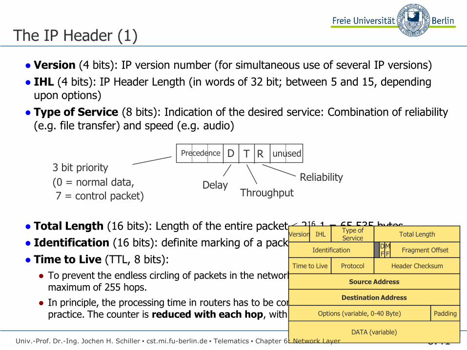
The IP Header (1)

● Version (4 bits): IP version number (for simultaneous use of several IP versions)

● IHL (4 bits): IP Header Length (in words of 32 bit; between 5 and 15, depending upon options)

● Type of Service (8 bits): Indication of the desired service: Combination of reliability

(e.g. file transfer) and speed (e.g. audio)

● Total Length (16 bits): Length of the entire packet 216-1 = 65,535 bytes

● Identification (16 bits): definite marking of a packet

● Time to Live (TTL, 8 bits):

● To prevent the endless circling of packets in the network the lifetime of packets is limited to a maximum of 255 hops.

● In principle, the processing time in routers has to be considered, which does not happen in practice. The counter is reduced with each hop, with 0 the packet is discarded.

Precedence D T R unused

3 bit priority (0 = normal data,

7 = control packet) Delay

Throughput

Reliability

Source Address


Total Length IHL



Destination Address


DATA (variable)

D F

M F


6.42

The IP Header (2)

● DF (1 bit): Don't Fragment. All routers must forward packets up to a size of 576

byte, everything beyond that is optional. Larger packets with set DF-bit therefore cannot take each possible way in the network.

● MF (1 bit): More Fragments

● “1” - further fragments follow

● “0” - last fragment of a datagram

● Fragment Offset (13 bits): Sequence number of the fragments of a packet (213 = 8192 possible fragments). The offset states, to which position of a packet

(counted in multiples of 8 byte) a fragment belongs to. From this a maximum

length of 8192 x 8 byte = 65,536 byte results for a packet.

● Protocol (8 bits): Which transport protocol is used in the data part (UDP, TCP,…)? To which transport process the packet has to be passed?

● Header Checksum (16 bits): 1’s complement of the sum of the 16-bit half

words of the header. Must be computed with each hop (since TTL changes)

● Source Address/Destination Address (32 bits): Network and host numbers

of sending and receiving computer. This information is used by routers for the

routing decision.

Source Address


Total Length IHL



Destination Address


DATA (variable)

D F

M F


6.43

Fragmentation

● A too large or too small packet length prevents a good performance. Additionally

there are often size restrictions (buffer, protocols with length specifications, standards, allowed access time to a channel,…)

● The data length must be a multiple of 8 byte. Exception: the last fragment, only

the remaining data are packed, padding to 8 byte units is not applied.

● If the “DF”-bit is set, the fragmentation is prevented.

777 x01 0 0 511

777 x01 64 512 1023

777 x00 128 1024 1200


777 x00 0 0 1200 bytes

IP header

ID Flags Offset Data

6.44

The IP Header (3)

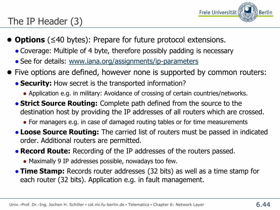
● Options (≤40 bytes): Prepare for future protocol extensions.

● Coverage: Multiple of 4 byte, therefore possibly padding is necessary

● See for details: www.iana.org/assignments/ip-parameters

● Five options are defined, however none is supported by common routers:

● Security: How secret is the transported information?

● Application e.g. in military: Avoidance of crossing of certain countries/networks.

● Strict Source Routing: Complete path defined from the source to the

destination host by providing the IP addresses of all routers which are crossed.

● For managers e.g. in case of damaged routing tables or for time measurements

● Loose Source Routing: The carried list of routers must be passed in indicated order. Additional routers are permitted.

● Record Route: Recording of the IP addresses of the routers passed.

● Maximally 9 IP addresses possible, nowadays too few.

● Time Stamp: Records router addresses (32 bits) as well as a time stamp for

each router (32 bits). Application e.g. in fault management.


http://www.iana.org/assignments/ip-parameters



6.45

Addressing



6.46

Classical IP Addressing

● Unique IP address for each host and router.

● IP addresses are 32 bits long and are used in the Source Address as well as in the Destination Address field of IP packets.

● The IP address is structured hierarchically and refers to a certain network, i.e., machines with connection to several networks have several IP addresses.

● Structure of the address: Network address for physical network (e.g. 160.45.117.0) and host address for a machine in the addressed network (e.g. 160.45.117.199)

32 bits

10 Network Host B

110 Network Host C 2,097,151 networks (LANs) with 256 hosts each (starting from 192.0.0.0)

0 Network Host

Class

A

1110 Multicast address D

1111 Reserved for future use E

16,383 networks with 216 hosts each (starting from 128.0.0.0)

126 networks with 224 hosts each (starting from 1.0.0.0)


6.47

147.216.113.y 192.168.13.x

IP Addresses

Binary format

Dotted Decimal Notation

11000000 . 10101000 . 00001101 . 00010101

192.168.13.21

192.168.13.1 147.216.113.1

147.216.113.71 192.168.13.21

● Each node has (at least) one world-wide unique IP address

● Router or gateways that link several networks, have for each network an IP address

192.168.13.0 147.216.113.0


6.48

IP Addresses and Routing

EthernetEthernet

Ethernet

Ethernet

Ethernet

Ethernet

Computer Server

Computer Computer

Computer

Computer

Computer

Computer

Computer

Computer

Computer

Computer

ComputerComputer

Server

Server

ServerServer Server

Server

Server

Server

Server

Server

147.216.0.0

142.117.0.0

12.0.0.0

194.52.124.0

a b

Destination IP Address

Connection Network Interface

12.x.x.x 194.52.124.x b

147.216.x.x 142.117.x.x a

142.117.x.x direct a

194.52.124.x direct b

x.x.x.x default a


6.49

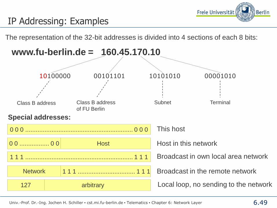
IP Addressing: Examples

Class B address Class B address

of FU Berlin

10100000 00101101 10101010 00001010

Subnet Terminal

The representation of the 32-bit addresses is divided into 4 sections of each 8 bits:

0 0 0 .............................................................. 0 0 0 This host

0 0 ................. 0 0 Host Host in this network

1 1 1 .............................................................. 1 1 1 Broadcast in own local area network

Network 1 1 1 ................................. 1 1 1 Broadcast in the remote network

127 arbitrary Local loop, no sending to the network

Special addresses:

www.fu-berlin.de = 160.45.170.10


6.50

Address Space

50%

25%

14%

6%

6%

Address Space

Class A

Class B

Class C

Class D

Class E


6.51

IP Addresses are scarce…

● Problems

● Nobody had thought about the explosive growth of the Internet (otherwise one would have defined longer addresses from the beginning).

● Too many Class A address blocks were assigned in the first Internet years.

● Inefficient use of the address space.

● Example: if 500 devices in an enterprise are to be attached, a Class B address

block is needed, but by this unnecessarily more than 65,000 host addresses are

blocked.

● Solution approach: Extension of the address space in IPv6

IP version 6 has 128 bits for addresses 2128 addresses

7 x 1023 IP addresses per square meter of the earth's surface (including the

oceans!)

one address per molecule on earth's surface!

● But: The success of IPv6 is not by any means safe!

● The introduction of IPv6 is tremendously difficult: Interoperability, costs,

migration strategies, …


6.52

Example for subnets: subnet mask 255.255.255.0

IP Subnets

● Problem: Class C-networks (256 hosts) are very small and Class B-

networks (65536 hosts) often too large

● Therefore, divide a network into subnets


Ethernet A 128.10.1.0

128.10.1.3 128.10.1.8 128.10.1.70 128.10.1.26

Ethernet B 128.10.2.0

128.10.2.3 128.10.2.133 128.10.2.18

128.10.2.1

All traffic for 128.10.0.0 Rest

of the Internet

Private Network

128.10.1.0 128.10.2.0 128.10.3.0 128.10.4.0

…

6.53

IP Subnets

● Within an IP network address block, several physical networks can be

addressed

● Some bits of the host address part are used as network ID

● A Subnet Mask identifies the “abused” bits

● All hosts of a network use the same subnet mask

● Routers can determine through combination of an IP address and a subnet

mask, to which subnet a packet must be sent


1 1 1 1 1 1 1 1 1 1 1 1 1 1 1 1 1 1 1 1 1 1 0 0 0 0 0 0 0 0 0 0 Subnet Mask

Network Host Class B address

10 Network Host Subnet

6.55

IP Subnets: Computation of the Destination

0111 1000 10100000

160 45 117 200

00101101 01110101 11001000

255 255 224 0

160 45 96 0

0000 0000

00000000

1110 0000

01100000

1111 1111

00101101

1111 1111

10100000

IP address

Subnet mask

Network of the addressed host

AND

The entrance router of the FU Berlin, which receives the IP packet, does not know, where host “117.200” is located.

A router computes the subnet “160.45.96.0” and sends the packet to the router, which links this subnet.


6.56

Classless Inter-Domain Routing (CIDR)

● Problem:

● Static categorization of IP addresses - how to use the very small class C networks efficiently?

● Remedy: Classless Inter-Domain Routing (CIDR)

● Weakening of the rigid categorization by replacing the static classes by network

prefixes of variable length

● Form of an IP address: a.b.c.d/n

● The first n bits are the network identification

● The remaining (32 – n) bits are the host identification

● Example: 147.250.3/17

● The first 17 bits are network ID and

the remaining 15 bits are host ID

● Used together with routing: Backbone router, e.g., on transatlantic links only

considers the first n bits; thus small routing tables, little cost of routing decision


10010011.11111010.00000011.00000000

Network ID Host ID

6.57

IPv6


6.58

IPv6 (December 1998, RFC 2460) IPv6 (December 1995, RFC 1883)

Publication of the standard (January 1995, RFC 1752)

Specification for IPng (December 1994, RFC 1726)

First requirements for IPng (December 1993, RFC 1550)

Simpler structure of the headers More automatism

Simpler configuration Performance improvements

Migration strategies More security

Larger address space

IPv4 (September 1981, RFC 791)

The new IP: IPv6


IPv6

ST-II (RFC1190) ST2+ (RFC 1819)

“IPv5” Stream oriented, never accepted,

concepts in MPLS, originally for voice

6.59

IPv6

● Why changing the protocol, when IPv4 works well?

● Dramatically increasing need for new IP addresses

● Improved support of real time applications

● Security mechanisms (Authentication and data protection)

● Differentiation of types of service, in particular for real time applications

● Support of mobility (hosts can go on journeys without address change)

● Simplification of the protocol in order to ensure a faster processing

● Reduction of the extent of the routing tables

● Option for further development of the protocol


6.60

Changes from IPv4 to IPv6

● Changes fall into following categories (RFC 1883, RFC 2460)

● Expanded Addressing Capabilities

● Header Format Simplification

● Improved Support for Extensions and Options

● Flow Labeling Capability

● Authentication and Privacy Capabilities


6.61

IPv6: Characteristics

● Address size

● 128-bit addresses (8 groups of each 4 hexadecimal numbers)

● Improved option mechanism

● Simplifies and accelerates the processing of IPv6 packets in routers

● Auto-configuration of addresses

● Dynamic allocation of IPv6-addresses

● Improvement of the address flexibility

● Anycast address: Reach any one out of several

● Support of the reservation of resources

● Marking of packets for special traffic

● Security mechanisms

● Authentication and Privacy

● Simpler header structure:

● IHL: redundant, no variable length of header by new option mechanism

● Protocol, fragmentation fields: redundant, moved into the options

● Checksum: Already done by layer 2 and 4


6.62

● Version: IP version number (4 bits)

● Traffic Class: classifying packets (8 bits)

● Flow label: virtual connection with certain characteristics/requirements (20 bits)

● PayloadLen: packet length after the 40-byte header (16 bits)

● Next Header: Indicates the type of the following extension header or the transport header (8 bits)

● HopLimit: At each node decremented by one. At zero the packet is discarded (8 bits)

● Source Address: The address of the original sender of the packet (128 bits)

● Destination Address: The address of the receiver (128 bits).

● Not necessarily the final destination, if there is an optional routing header

● Next Header/Data: if an extension header is specified, it follows after the main header. Otherwise, the data are following

1 4 8 32 16 24

The prefix of an address characterizes geographical areas, providers, local internal areas,…

IPv6 Header

Version (4)

Next Header (8) HopLimit (8) PayloadLen (16)

Flow label (20)

Next Header/Data

Traffic Class (8)

Source Address (128)

Destination Address (128)


6.63

IPv6 Header

● Packet size requirements

● IPv6 requires that every link has MTU ≥ 1280 bytes

● Links which cannot convey 1280 byte packets has to apply link-specific

fragmentation and assembly at a layer below IPv6

● Links that have a configurable MTU must be configured to have an MTU of at

least 1280 bytes

● It is recommended that they be configured with an MTU ≥ 1500 bytes


6.64

IPv4 vs. IPv6: Header

En sion

Prio rity

Flow label

PayloadLen NEXT headers

Hop limit

Source Address

Destination Address

Next Header / Data

SOURCE ADDRESS

Destination ADDRESS

Destination ADDRESS

Destination ADDRESS

Destination ADDRESS

NEXT header/DATA

En sion

IHL Totally length Type OF service

Identification Fragment offset

Time to Live

Protocol Header Checksum

SOURCE ADDRESS

Destination ADDRESS

Option (variable)/Padding

DATA

The IPv6 header is longer, but this is only caused by the longer addresses. Otherwise it is “better sorted” and thus faster to process by routers.

Ver- sion

4 8 16 32

Traffic Class

Flow Label

PayloadLen Next

Header Hop Limit

Next Header / Data

4 8 16 32

Ver- sion

IHL Total Length Type of Service

Identification

Time to Live

Protocol

Source Address

Destination Address

Options (variable)/Padding

Data

Source Address

Destination Address


6.65

IPv6 Path MTU Discovery

● Path MTU Discovery

● MTU: Maximum Transmission Unit

● Maximum packet size in octets, that can be conveyed in one piece over a link

● Path MTU: The minimum link MTU of all the links in a path between a source

node and a destination node

● Path MTU Discovery Process

● The originating node assumes the Path MTU is the MTU of the first hop in the

path.

● A trial packet of this size is sent out.

● If any link is unable to handle it, an ICMPv6 Packet Too Big message is returned.

● The originating node iteratively tries smaller packet sizes until it gets no complaints from any node, and then uses the largest MTU that was acceptable

along the entire path.


6.66

Extension Headers

IPv6


6.67

IPv6 Extension Headers

● Optional data follows in extension headers. There are 6 headers defined:

● Hop-by-Hop (information for single links) All routers have to examine this field.

● Momentarily only the support of Jumbograms (packets exceeding the normal IP packet

length) is defined (length specification).

● Routing (definition of a full or partly specified route)

● Fragment (administration of fragments)

● Difference to IPv4: Only the source can do fragmentation. Routers for which a packet is too large, only send an error message back to the source.

● Authentication (of the sender)

● Encapsulating security payload (information about the encrypted payload)

● Destination options (additional information for the destination)

● Each extension should occur at most once!


6.68


● Examples for the use of extension headers:


IPv6 header Next Header = TCP

TCP header + data

IPv6 header Next Header = Routing

Routing header Next Header = TCP

TCP header + data

IPv6 header Next Header = Routing

Routing header Next Header = Fragment

Fragment header Next Header = TCP

TCP header + data

6.69


● Two extension headers can carry a variable number of type-length-value

(TLV) optins

● Hop-by-Hop

● Destination options

● Options are encoded as:

● Option Type determines also the action that must be taken if the processing IPv6

node does not recognize the Option Type

● The highest-order two bits specifies the action

- 00: skip over this option and continue processing the header

- 01: discard the packet

- 10: discard the packet and ICMP message to source (unicast and multicast)

- 11: discard the packet and ICMP message to source (only unicast)


Option Type Opt Data Len Option Data

6.70

Addressing

IPv6


6.71

IPv6 Addresses (RFC 4291)

● IPv6 Addresses are longer

● 128 bit = 16 byte

● 2128 addresses ~ 3.4×1038

● Three types of addresses

● Unicast: An identifier for a single interface.

● Anycast: An identifier for a set of interfaces. A packet sent to an anycast address

is delivered to the “nearest” one.

● Multicast: An identifier for a set of interfaces. A packet sent to a multicast

address is delivered to all interfaces identified by that address.

● There are no broadcast addresses in IPv6!

● Their function are superseded by multicast addresses


6.72

IPv6 Addresses: Representation of addresses

● The preferred form is

x:x:x:x:x:x:x:x

● the 'x's are the hexadecimal values of the eight 16-bit pieces of the address

● Written as eight groups of four hexadecimal digits with colons as separators

● Examples:

8000:0000:0000:0000:0123:4567:89AB:CDEF

FEDC:BA98:7654:3210:FEDC:BA98:7654:3210

1080:0:0:0:8:800:200C:417A


6.73


● Some simplifications

● Leading zeros within a group can be omitted: 0123 123

● Groups of 16 zero bits ‘0000’ can be replaced by a pair of colons ‘::’

8000:0000:0000:0000:0123:4567:89AB:CDEF 8000::123:4567:89AB:CDEF

● The "::" can only appear once in an address

● Example:

The following addresses

2001:DB8:0:0:8:800:200C:417A a unicast address

FF01:0:0:0:0:0:0:101 a multicast address 0:0:0:0:0:0:0:1 the loopback address

0:0:0:0:0:0:0:0 the unspecified addresses

may be represented as

2001:DB8::8:800:200C:417A a unicast address

FF01::101 a multicast address ::1 the loopback address

:: the unspecified addresses


6.74


● Usage of IPv4 addresses together with IPv6 addresses as

x:x:x:x:x:x:d.d.d.d

● the 'x's are the hexadecimal values of the six high-order 16-bit pieces of the

address, and the 'd's are the decimal values of the four low-order 8-bit pieces of

the address (standard IPv4 representation)

● Examples:

● 0:0:0:0:0:0:13.1.68.3

● 0:0:0:0:0:FFFF:129.144.52.38

● or in compressed form:

● ::13.1.68.3

● ::FFFF:129.144.52.38


6.75


● The text representation of IPv6 address prefixes is similar to the way IPv4

address prefixes are written in Classless Inter-Domain Routing (CIDR)

ipv6-address/prefix-length

● ipv6-address: an IPv6 address

● prefix-length: number of bits comprising the prefix (leftmost contiguous)

● Examples: 60-bit prefix 20010DB80000CD3 (hexadecimal)

2001:0DB8:0000:CD30:0000:0000:0000:0000/60

2001:0DB8::CD30:0:0:0:0/60

2001:0DB8:0:CD30::/60

● Combination of node address and a prefix:

● node address 2001:0DB8:0:CD30:123:4567:89AB:CDEF

● subnet number 2001:0DB8:0:CD30::/60

Abbreviated to: 2001:0DB8:0:CD30:123:4567:89AB:CDEF/60


6.76

IPv6 Addresses: Address Types

● The type of an IPv6 address is identified by the high-order bits of the

address:

● Unspecified: It must never be assigned to any node. It indicates the absence of

an address. Used when host initializes and does not have an address.

● Loopback: It may be used by a node to send an IPv6 packet to itself. It must not

be assigned to any physical interface.


Address type Binary prefix IPv6 notation

Unspecified 00...0 (128 bits) ::/128

Loopback 00...1 (128 bits) ::1/128

Multicast 11111111 FF00::/8

Link-Local unicast 1111111010 FE80::/10

Global Unicast (everything else)

6.77


● Global Unicast Addresses

● The general format for IPv6 Global Unicast addresses is as follows:

● global routing prefix: required for routing in a site

● subnet ID: identifier of a link within the site


n bits m bits 128-n-m bits

global routing prefix subnet ID interface ID

6.78


● Anycast Addresses

● Anycast addresses are allocated from the unicast address space

● Anycast addresses are syntactically indistinguishable from unicast addresses

● When a unicast address is assigned to more than one interface, thus it becomes

an anycast address

● Usage scenarios:

● Identifaction of the set of routers belonging to an organization providing Internet

service

● Identifaction of the set of routers attached to a particular subnet

● Identifaction of the set of routers providing entry into a particular routing domain

● Format:


n bits 128-n bits

subnet prefix 00000000000000

6.79


● Multicast Addresses:

● An IPv6 multicast address is an identifier for a group of interfaces

● An interface may belong to any number of multicast groups.

● Format:

● 11111111: identification of multicast addresses

● flgs: set of 4 flags: 0RPT

● T=0: permanently assigned multicast address

● T=1: non-permanently assigned multicast address

(dynamically, on-demand)

● P: multicast address assignment based on network

prefix (RFC 3306)

● R: embedding of the rendevous point (RFC 3956)

● scop: limit the scope of the multicast group


8 4 4 112 bits

11111111 flgs scop group ID Scope values (4 bit) 0 reserved 1 Interface-Local scope 2 Link-Local scope 3 reserved 4 Admin-Local scope 5 Site-Local scope 6 (unassigned) 7 (unassigned) 8 Organization-Local scope 9 (unassigned) A (unassigned) B (unassigned) C (unassigned) D (unassigned) E Global scope F reserved

6.80

Transition from IPv4 to IPv6

IPv6


6.81


● IPv6 cannot be introduced “over night”… for some time both IP variants

will be used in parallel.

● Nearly all operating systems support both IP variants

● Only the infrastructure nodes has to be updated

● But: how to enable two modern IPv6-based hosts to communicate if only an

IPv4-based network is in between?

Transition methods

● Several transitions methods proposed

● Co-existence of IPv4 and IPv6

● Translation

● Tunneling


6.82


● Co-existence of IPv4 and IPv6

● Co-existence involves all client and server nodes supporting both IPv4 and IPv6

● Running essentially two complete networks that share the same infrastructure

● Dual Stack


Application Layer

TCPv4, UDPv4

IPv4, ICMPv4

Host-to-Network Layer

TCPv6, UDPv6

IPv6, ICMPv6

6.83


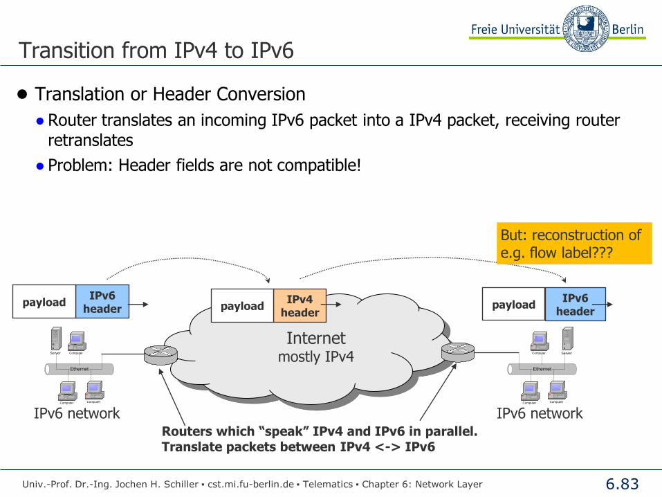
● Translation or Header Conversion

● Router translates an incoming IPv6 packet into a IPv4 packet, receiving router retranslates

● Problem: Header fields are not compatible!


Internet mostly IPv4

Ethernet

ComputerServer

Computer Computer

IPv6 network

IPv6 header

payload IPv4 header

payload IPv6

header payload

Ethernet

Computer Server

Computer Computer

IPv6 network

But: reconstruction of e.g. flow label???

Routers which “speak” IPv4 and IPv6 in parallel. Translate packets between IPv4 <-> IPv6

6.84


● Tunneling

● Router at the entry to the IPv4-based network encapsulates an incoming IPv6 packet into a new IPv4 packet with destination address of the next router also

supporting IPv6


Internet mostly IPv4

Ethernet

ComputerServer

Computer Computer

IPv6 network

IPv6 header

payload IPv4 header

Ethernet

Computer Server

Computer Computer

IPv6 network

●More overhead because of two headers for one packet, but no information loss ● Tunneling is a general concept also used for multicast, VPN, etc: it simply means

“pack a whole packet as it is into a new packet of different protocol”

IPv6 “tunnel” through IPv4

IPv6 header

payload IPv6

header payload

6.85

Network Address Translation (NAT)


6.86


● Problem: IP addresses are scarce, thus not every node gets an public IP address

● Approach: Special IP addresses that must no be used in the global public Internet, but can be used in an Intranet

● Each internal computer in the Intranet needs an own IP address to communicate with the others.

● For this purpose, “private” address blocks are reserved ● 10.0.0.0 – 10.255.255.255

● 172.16.0.0 – 172.31.255.255

● 192.168.0.0 – 192.168.255.255

● When using addresses of those ranges, the internal computers can communicate with each other


Internet

Public Internet with global IP addresses

• Intranet with private IP addresses

•Each node in the Intranet has a unique IP address

•Device with global public IP address and private IP address

•Translates private to public addresses

6.87


● Packets with private IP addresses are not forwarded by a router

● Thus: routers, which are attached to the “external world” need a global address

● Assign a few IP addresses to a company which are known by a “NAT box” which usually is installed with the router

● When data are leaving the own network, an address translation takes place: the NAT box exchanges the private address with a globally valid one

● Side effect: hiding of the internal network structure (security)


Internet

Public Internet with global IP addresses

•Structure of the Intranet is hidden from the global Internet

•Connections from global Internet not possible

NAT box

6.88

NAT Variants

● NAT is available in several “variants”, known under different names

● Basic NAT (also: Static NAT) ● Each private IP address is translated into one certain external IP address

● Either, you need as much external addresses as private ones, otherwise no re-translation is possible when a reply arrives

● Or, you manage a pool of external IP addresses and assign one dynamically when a request is sent out

Ethernet

ComputerServer

Computer Computer

router with NAT box

Internet

192.168.0.2 192.168.0.3

192.168.0.4 192.168.0.5

Ethernet

ComputerServer

Computer Computer

router with NAT box

Internet

192.168.0.2 192.168.0.3

192.168.0.4 192.168.0.5

Private IP Map to

192.168.0.2 147.216.13.32

192.168.0.3 147.216.13.33

192.168.0.4 147.216.13.34

192.168.0.5 147.216.13.35

Private IP Currently

mapped:

192.168.0.2 147.216.13.32

192.168.0.5 147.216.13.33

--- 147.216.13.34

--- 147.216.13.35


6.89

NAT Variants

● Disadvantages of static NAT:

● With static mapping, you need as much public IP addresses as you have computers

● With dynamic mapping, you need less public IP addresses, but for times of high

traffic you nevertheless need nearly as much addresses as local computers

● Those approaches help to hide the network structure, but not to save addresses

● Hiding NAT (also: NAPT: Network Address Port Translation, Masquerading)

● Translates several local addresses into the same external address

● Now: some more details are necessary to deliver a response

Ethernet

ComputerServer

Computer Computer

router with NAT box

Internet

192.168.0.2 192.168.0.3

192.168.0.4 192.168.0.5

Private IP Map to

192.168.0.2 147.216.12.32

192.168.0.3 147.216.12.32

192.168.0.4 147.216.12.32

192.168.0.5 147.216.12.32

to: 147.216.12.32

destination?


6.90

Network Address Port Translation (NAPT)

Protocol Port

(local)

IP

(local)

Port

(global)

IP

(global)

IP

(destination)

Port (destination)

TCP 1066 10.0.0.1 1066 198.60.42.12 147.216.12.221 21

TCP 1500 10.0.0.7 1500 198.60.42.12 207.17.4.21 80


6.91

Problems with NAPT

● NAPT works well with communication initiated from the Intranet.

● But: how could someone from outside give a request to the Intranet (e.g.

to the web server)?

● NAPT box needs to be a bit more “intelligent”

● Some static information has to be stored, e.g., “each incoming request with port

80 has to be mapped to the private address of the web server”

● Still problems with applications like ICQ

● Thus, only more IP addresses really help to solve the problem


6.92

Even more NAT versions…

● Carrier Grade NAT (CGN)

● Also known as LSN (Large Scale NAT)

● Use a NAT box for a larger number of customers, e.g., a street, a suburb to

further mitigate IPv4 address exhaustion

● Again – breaks end-to-end principle, difficult to use well-known ports etc.

● NAT64 (RFC 6146)

● Mechanism to connect IPv6 hosts to IPv4 servers

● IPv6 client embeds IPv4 address (RFC 6052)

● NAT maps IPv6 to IPv4


6.93

ARP, RARP, DHCP, ICMP

Auxiliary Protocols


6.94

Internet Layer







IPv4, IPv6


Routing Tables

6.95

Auxiliary Protocols

● IP serves only for sending packets with well-known addresses. Some

questions however remain open, which are handled by auxiliary protocols:

● Address Resolution Protocol (ARP)

● Reverse Address Resolution Protocol (RARP)

● Internet Control Message Protocol (ICMP)

● Internet Group Management Protocol (IGMP)


6.96

Delivery of Packets

Ethernet

Ethernet

Computer

Computer

ComputerComputer

ServerServer Server

Server

142.117.0.0

194.52.124.0

194.52.124.1

194.52.124.10

142.117.1.7

142.117.1.1

AL

TL

NL IP Addresses

DL MAC Addresses

PL


6.97

Delivery of IP Packets

● Address Resolution Protocol (ARP)

● The Internet is a virtual network, which is build upon physical networks.

● IP addresses only offer a logical address space

● The hardware on the lower layers do not understand IP addresses

● Within a local area network, the sender must know the hardware address (MAC address) of the receiver before sending an IP packet to the destination host

● The hardware address is with Ethernet an 48-bit address, which is assigned

to a network interface card (NIC) by the manufacturer

● With ARP, IP is mapped to the hardware address and vice versa

● ARP uses the local broadcast address to dynamically inquire for the hardware

address by indication of the searched IP address

● An ARP request is only valid in the local network


6.98

Address Resolution Protocol (ARP)

ARP Request

A B C D E

192.168.13.18 192.168.13.142 192.168.13.1 192.168.13.51 192.168.13.20

Look for the physical address to the IP address 192.168.13.20

17 54 143 97 62

20

20?

20?

62

20? 20?

ARP Response The physical address to the IP address 192.168.13.20 is 62

The host with the inquired IP address sends a response

Each host stores well-known IP and hardware addresses in a table

The entries become invalid after a certain time to avoid mistakes e.g. with the exchange of a network interface card

A B C D E

ARP Response

●The host with the inquired IP address sends a response

●Each host stores familiar IP and MAC addresses in a table

●The entries become invalid after a certain time to avoid mistakes e.g. with the exchange of a network interface card

192.168.13.18 192.168.13.142 192.168.13.1 192.168.13.51 192.168.13.20

17 54 143 97 62

The physical address to the IP address 192.168.13.20 is 62

ARP Request

A B C D E

192.168.13.18 192.168.13.142 192.168.13.1 192.168.13.51 192.168.13.20

Look for the physical address to the IP address 192.168.13.20

17 54 143 97 62


6.99

Optimization of the procedure:

Each computer occasionally sends an ARP request (broadcast) to its own IP

address.

ARP Request

A B C D E

Each receiving host stores the sender IP and sender hardware address in its ARP Cache

Address Resolution Protocol (ARP)


6.100

Reverse Address Resolution Protocol (RARP)

● Not with all operating systems an IP address is assigned to a computer during startup. How does such a computer receive its IP address after booting?

● With the help of Reverse ARP, well-known hardware addresses are assigned to IP-addresses.

● RARP makes it possible that a booted machine broadcasts its hardware address and gets back by a RARP server the appropriate IP address.

RARP Request

A B C D E RARP server

I have the hardware address 62 The IP address is 192.168.13.20

62

62 62 62

20

RARP Request

A B C D E

I have the hardware address 62

The IP address is 192.168.13.20


6.101

Dynamic Host Configuration Protocol

(DHCP)


6.102

Dynamic Host Configuration Protocol (DHCP)

● Problem with RARP: RARP requests are not passed on by routers, therefore an own RARP server must be set up in each local network.

● Solution: DHCP. A computer sends a DHCP DISCOVER packet. In each subnet a DHCP Relay Agent is placed, who passes such a message on to the DHCP server.

●Additionally to the IP address also the subnet mask, domain names, … are transferred. Thus, DHCP can be used for full host configuration.


6.103

Dynamic Host Configuration Protocol (DHCP)


DHCP server 223.1.2.5

Client DHCP discover src : 0.0.0.0:68

dest.: 255.255.255.255:67

yiaddr: 0.0.0.0

transaction ID: 654

DHCP offer src: 223.1.2.5:67

dest: 255.255.255.255:68

yiaddrr: 223.1.2.4

transaction ID: 654

Lifetime: 3600 secs

DHCP request src: 0.0.0.0:68

dest:: 255.255.255.255:67

yiaddrr: 223.1.2.4

transaction ID: 655

Lifetime: 3600 secs

DHCP ACK src: 223.1.2.5:67

dest: 255.255.255.255:68

yiaddrr: 223.1.2.4

transaction ID: 655

Lifetime: 3600 secs

6.104

Internet Group Management Protocol

(IGMP)


6.105

How to realize Multicast with IPv4?

Unicast is an end-to-end transmission between two hosts.

Multiple transmissions have to be executed sequentially.

For multicast, data is replicated by the network and send in parallel.

Inefficient use of time and capacities.

Sender

Receiver

Receiver

1. Transmission

2. Transmission

Unicast

Broadcast is a one-to-all transmission

A packet is sent to all possible receivers , many of them may not need it

Network load by use of transmission paths, which are not needed actually

Problem with Unicast and Broadcast:

How can a group of computers be

addressed efficiently?


Broadcast

Receiver Receiver

Receiver Receiver

Sender

6.106

IP Multicast

Transmission to n > 1 selected stations: Multicast

Problems:

Support of multicast is not compulsory required to be supported by all devices in IPv4, mandatory in IPv6

Efficient addressing: how to arrange to reach exactly the desired devices?

IPv4:

Use of multicast addresses: Class D addresses, from 224.0.0.0 to 239.255.255.255

Some of them are reserved for certain purposes (e.g. 224.0.0.2 - all gateways in the subnet)

Standard IP functionality is enhanced by functions of the Internet Group Management Protocol (IGMP) for IPv4 and Multicast Listener Discovery (MLD) for IPv6

How can a limited group of computers be addressed with something between unicast and broadcast?


Receiver

Multicast

Receiver

Sender

6.107

Internet Group Management Protocol (IGMP)

● For delivery of multicast messages to all group members that are located in

different physical networks, routers need information about group associations.

● If groups are only temporary, routers have to acquire information about

associated hosts by themselves.

● By means of IGMP messages (encapsulated into IP packets), a router informs all hosts in its subnet to which groups they belong

● Routers notice the existence of group members

● Periodically, the routers ask (Polling), which groups of multicast are still present

● Routers exchange information to build multicast routing trees


Multicast router Group

members

6.108

Multicast Control Path – an example

IGMP message

Routing information

Router

Host

The routers exchange their routing information

By means of IGMP messages, group associations are being passed on

To each multicast address the routers administrate routing information

At least one participant

No participant here

Sender

Find shortest paths

Pruning Messages (Unnecessary branches are cut off)

The routing protocol computes the shortest paths to all computers in the network

Routers, which do not have participants in their network, can send back Pruning Messages; next time no more multicast packets are sent to this routers


Details vary by the specific protocol used!

6.109

Multicast Groups: Example

Network with interest into two multicast groups

Sink Tree for the left router

Multicast routing tree for group 1 Multicast routing tree for group 2


6.110

Multicast Routing – PIM-SM as example

● Protocol Independent Multicast – Sparse Mode (RFC 2362)

● Can support Internet-wide MC groups, does not require specific unicast protocol

● No flooding plus pruning but explicit construction of a tree

● Assumptions

● Only a very low percentage of nodes will subscribe to a MC group

● Joining an MC group

● IGMP join in the local subnet

● PIM join to a so-called rendezvous point (RP)

● PIM join between RP and sender

● Routers forward join messages to an RP

● MC sender

● Send register messages to RP

● RP distributes data along MC tree


6.111

Internet Control Message Protocol (ICMP)


6.112

Internet Control Message Protocol (ICMP)

● ICMP is a control protocol of layer 3, which is build upon IP! This protocol

is used e.g. by routers, if something unexpected happens, like TTL=0.

● Example 1: if a router cannot forward a packet, the source can be

informed about it. ICMP messages are in particular helpful in the case of

failures in the network.

● Example 2: ping (question about a life sign of a station) uses ICMP

messages.


Router

ICMP Message

ICMP Request

ICMP Reply

Router

Host

Host

ICMP Request: status request

ICMP Reply: status reply

ICMP Message: Transmission of status

information and control

messages

6.113

ICMP: Header

● ICMP message fields

● Type: purpose of the ICMP message

● Around 40 defined ICMP message types

● Types 41 – 255 for future use

● Code: additional information about the condition

● Very rarely used

● Checksum: same type of checksum as used for IP

● Message categories

● Error messages: to report an event. These messages do not have a response.

● Error messages include the IP header that generated the error!

● Queries: To get some information from a node. These messages have a matching response.


1 byte 1 byte 2 byte

Type Code Checksum

ICMP Data (content and format depends on Type)

General format of ICMP messages


Type =3 Code Checksum

Unused (all 0 bits)

IP Header (20 bytes) and

First 8 bytes of original packet data

Format of Destination Unreachable ICMP message

6.114

ICMP: Header

● ICMP transmits error and control messages on the network level. These

messages are sent in an IP packet

● Type/code indicates the type (and format) of the message, e.g.:


Type Meaning

0 Destination unreachable (packet cannot be sent)

3 Echo request/reply (status request, e.g. for ping)

4 Source Quench (Choke packet, data rate reduction)

11 Time exceeded for datagram (TTL = 0, the packet is discarded)

12 Parameter problem on datagram (A header field is set wrongly)

15/16 Information Request/Reply

30 Trace route (Trace the network path)

6.115

ICMP: Applications

● Some very popular applications of ICMP

● Ping

● Traceroute

● Path MTU


6.116

ICMP & IPv6

● ICMPv6 introduces some changes to ICMP

● New ICMPv6 messages and procedures replace ARP

● There are ICMPv6 messages to help with automatic address configuration

● Path MTU discovery is automatic

● New PacketTooBig message is sent to the source, since IPv6 routers do not fragment

● There is no Source Quench in ICMPv6

● IGMP for multicast is included in ICMPv6 (Multicast Listener Discovery, RFC4604)

● ICMPv6 helps detect nonfunctioning routers and inactive partner hosts



Type Code Checksum

Message Body

General format of ICMPv6 messages

6.117

Some Tools


6.118

Some Tools: Arp

● Arp

● Display and insert entries into the arp cache

x:\>arp -a Interface: 160.45.114.21 --- 0x2 Internet Address Physical Address Type 160.45.114.1 00-12-79-8d-68-00 dynamic 160.45.114.28 00-14-32-49-c1-aa dynamic 160.45.114.29 00-04-15-d8-53-cb dynamic 160.45.114.30 00-04-85-8b-9a-ac dynamic 160.45.114.31 00-19-f9-18-82-3d dynamic 160.45.114.34 00-04-25-8b-a8-8e dynamic


6.119

Some Tools: Route

● Route

● Display and set routing table entries

x:\>route PRINT =========================================================================== Interface List 0x1 ........................... MS TCP Loopback interface 0x2 ...00 1a a0 b7 41 39 ...... Broadcom NetXtreme 57xx Gigabit Controller =========================================================================== =========================================================================== Active Routes: Network Destination Netmask Gateway Interface Metric 0.0.0.0 0.0.0.0 160.45.114.1 160.45.114.21 10 127.0.0.0 255.0.0.0 127.0.0.1 127.0.0.1 1 160.45.114.0 255.255.255.192 160.45.114.21 160.45.114.21 10 160.45.114.21 255.255.255.255 127.0.0.1 127.0.0.1 10 160.45.255.255 255.255.255.255 160.45.114.21 160.45.114.21 10 224.0.0.0 240.0.0.0 160.45.114.21 160.45.114.21 10 255.255.255.255 255.255.255.255 160.45.114.21 160.45.114.21 1 Default Gateway: 160.45.114.1 =========================================================================== Persistent Routes: None


6.120

Some Tools: Ping

● Ping

● Tool to test whether a host is reachable/alive

x:\>ping www.google.com Pinging www.l.google.com [209.85.135.104] with 32 bytes of data: Reply from 209.85.135.104: bytes=32 time=26ms TTL=243 Reply from 209.85.135.104: bytes=32 time=24ms TTL=243 Reply from 209.85.135.104: bytes=32 time=23ms TTL=243 Reply from 209.85.135.104: bytes=32 time=24ms TTL=243 Ping statistics for 209.85.135.104: Packets: Sent = 4, Received = 4, Lost = 0 (0% loss), Approximate round trip times in milli-seconds: Minimum = 23ms, Maximum = 26ms, Average = 24ms


6.121

Some Tools: Traceroute

● Traceroute/tracert

● Tool to determine the used path in the Internet

x:\>tracert www.google.com Tracing route to www.l.google.com [209.85.135.104] over a maximum of 30 hops: 1 <1 ms <1 ms <1 ms router-114.mi.fu-berlin.de [160.45.114.1] 2 <1 ms <1 ms <1 ms pollux.mi.fu-berlin.de [160.45.113.243] 3 <1 ms <1 ms <1 ms zedat.router.fu-berlin.de [160.45.252.181] 4 307 ms <1 ms <1 ms ice2.spine.fu-berlin.de [130.133.98.3] 5 <1 ms <1 ms <1 ms xr-zib1-ge8-3.x-win.dfn.de [188.1.33.46] 6 * * * Request timed out. 7 18 ms 15 ms 15 ms zr-fra1-te0-0-0-3.x-win.dfn.de [80.81.192.222] 8 28 ms 15 ms 15 ms de-cix10.net.google.com [80.81.192.108] 9 16 ms 16 ms 15 ms 209.85.255.172 10 24 ms 23 ms 24 ms 72.14.233.106 11 24 ms 24 ms 23 ms 66.249.94.83 12 26 ms 27 ms 26 ms 209.85.253.22 13 24 ms 24 ms 24 ms mu-in-f104.google.com [209.85.135.104] Trace complete.


6.122

Some Tools: Pathping (1)

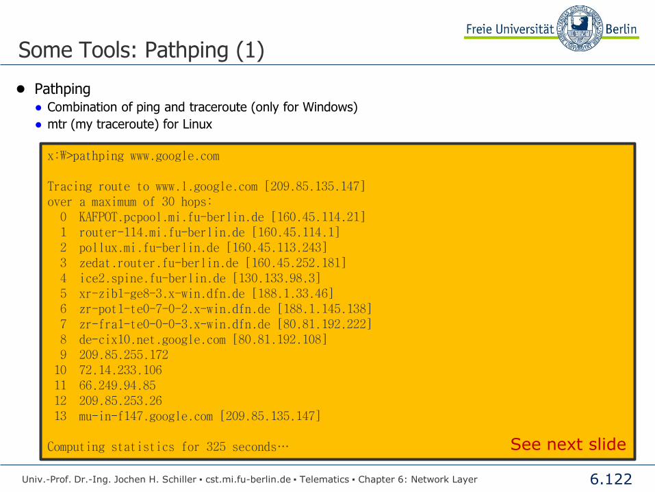
● Pathping ● Combination of ping and traceroute (only for Windows)

● mtr (my traceroute) for Linux

x:\>pathping www.google.com Tracing route to www.l.google.com [209.85.135.147] over a maximum of 30 hops: 0 KAFPOT.pcpool.mi.fu-berlin.de [160.45.114.21] 1 router-114.mi.fu-berlin.de [160.45.114.1] 2 pollux.mi.fu-berlin.de [160.45.113.243] 3 zedat.router.fu-berlin.de [160.45.252.181] 4 ice2.spine.fu-berlin.de [130.133.98.3] 5 xr-zib1-ge8-3.x-win.dfn.de [188.1.33.46] 6 zr-pot1-te0-7-0-2.x-win.dfn.de [188.1.145.138] 7 zr-fra1-te0-0-0-3.x-win.dfn.de [80.81.192.222] 8 de-cix10.net.google.com [80.81.192.108] 9 209.85.255.172 10 72.14.233.106 11 66.249.94.85 12 209.85.253.26 13 mu-in-f147.google.com [209.85.135.147] Computing statistics for 325 seconds… See next slide


6.123

Some Tools: Pathping (2)

Computing statistics for 325 seconds... Source to Here This Node/Link Hop RTT Lost/Sent = Pct Lost/Sent = Pct Address 0 KAFPOT.pcpool.mi.fu-berlin.de [160.45.114.21] 0/ 100 = 0% | 1 0ms 0/ 100 = 0% 0/ 100 = 0% router-114.mi.fu-berlin.de [160.45.114.1] 0/ 100 = 0% | 2 0ms 0/ 100 = 0% 0/ 100 = 0% pollux.mi.fu-berlin.de [160.45.113.243] 0/ 100 = 0% | 3 3ms 0/ 100 = 0% 0/ 100 = 0% zedat.router.fu-berlin.de [160.45.252.181] 0/ 100 = 0% | 4 0ms 0/ 100 = 0% 0/ 100 = 0% ice2.spine.fu-berlin.de [130.133.98.3] 0/ 100 = 0% | 5 0ms 0/ 100 = 0% 0/ 100 = 0% xr-zib1-ge8-3.x-win.dfn.de [188.1.33.46] 0/ 100 = 0% | 6 1ms 0/ 100 = 0% 0/ 100 = 0% zr-pot1-te0-7-0-2.x-win.dfn.de [188.1.145.138] 0/ 100 = 0% | 7 14ms 93/ 100 = 93% 93/ 100 = 93% zr-fra1-te0-0-0-3.x-win.dfn.de [80.81.192.222] 0/ 100 = 0% | 8 17ms 0/ 100 = 0% 0/ 100 = 0% de-cix10.net.google.com [80.81.192.108] 0/ 100 = 0% | 9 20ms 0/ 100 = 0% 0/ 100 = 0% 209.85.255.172 0/ 100 = 0% | 10 24ms 0/ 100 = 0% 0/ 100 = 0% 72.14.233.106 0/ 100 = 0% | 11 29ms 0/ 100 = 0% 0/ 100 = 0% 66.249.94.85 0/ 100 = 0% | 12 28ms 0/ 100 = 0% 0/ 100 = 0% 209.85.253.26 1/ 100 = 1% | 13 24ms 1/ 100 = 1% 0/ 100 = 0% mu-in-f147.google.com [209.85.135.147] Trace complete.


6.124

Routing


6.125

Internet Layer







IPv4, IPv6


Routing Tables

6.126

Routing Tables

EthernetEthernet

Ethernet

Ethernet

Ethernet

Ethernet

Computer Server

Computer Computer

Computer

Computer

Computer

Computer

Computer

Computer

Computer

Computer

ComputerComputer

Server

Server

ServerServer Server

Server

Server

Server

Server

Server

157.216.0.0

142.117.0.0

12.0.0.0

194.52.124.0

194.52.124.1

Destination Address Next Hop

12.0.0.0/8 194.52.124.1

157.216.0.0/16 142.117.1.1

142.117.0.0/16 142.117.1.1

194.52.124.0/24 194.52.124.1

0.0.0.0/0 142.117.1.1

194.52.124.10

142.117.1.7

142.117.1.1


6.127

Routing in the Internet

● The Internet consists of a large number of Autonomous Systems (AS)

● Each autonomous system is operated by its operator and can deploy a routing protocol

● By standardization of protocols, gateways can forward packets at the borders of the autonomous systems


Internal

Protocol 1

Internal

Protocol 3

Internal

Protocol 2

Autonomous Systems

External Protocol

AS1

AS2

AS3

6.128

Routing Protocols

● Interior Gateway Protocols (IGP):

Routing in autonomous systems, for efficient transmission

● Routing Information Protocol (RIP)

● Internet Gateway Routing Protocol (IGRP)

● Enhanced IGRP


● Intermediate System to Intermediate System (IS-IS)

● Exterior Gateway Protocols (EGP):

Routing between domains, adherence of policies for the domains


● Router Discovery Protocols

● ICMP Router Discovery Protocol (IRDP)

● Hot Standby Router Protocol (HSRP)


6.129

Routing in a Sub-Network

● Sub-network consists of many

routers

● Routers are connected by several

links

● Connections are partially

redundant

● Connections have different

characteristics

● Speed, Delay, etc.

● Therefore “optimization” of the

routes by elimination of long

paths


H

J

C A

B

D

I

E

F G

K

L

M

N

O

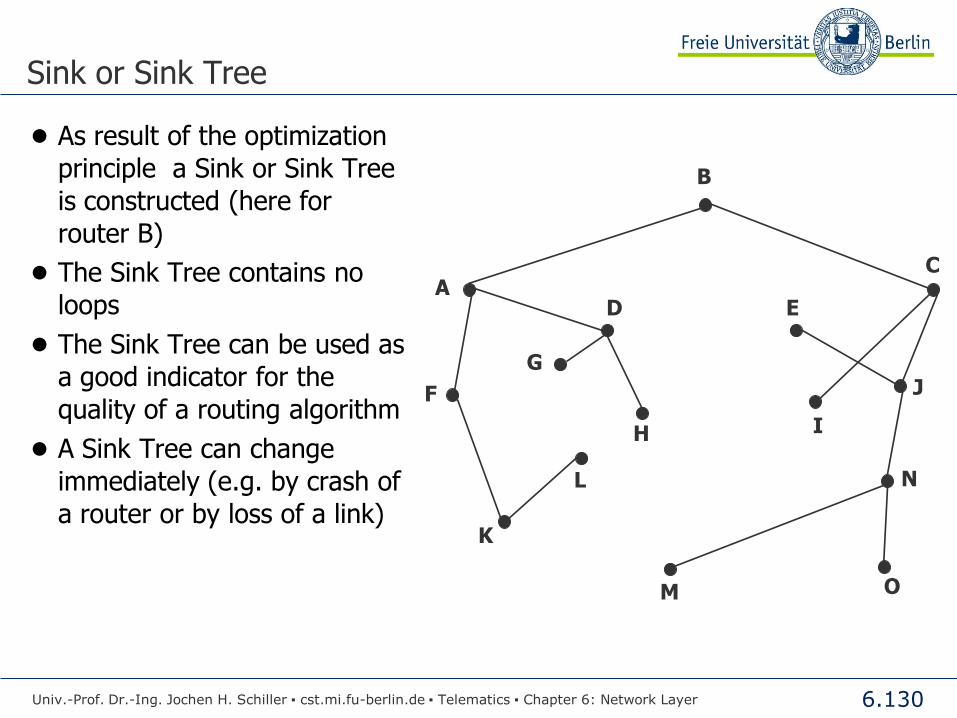
6.130

H

J

C A

B

D

I

E

F

G

K

L

M

N

O

Sink or Sink Tree

● As result of the optimization

principle a Sink or Sink Tree

is constructed (here for

router B)

● The Sink Tree contains no

loops

● The Sink Tree can be used as

a good indicator for the

quality of a routing algorithm

● A Sink Tree can change

immediately (e.g. by crash of

a router or by loss of a link)


6.131

Routing Algorithms: Graph abstraction

● Abstraction of a computer network as a graph

● Graph: G = (N, E)

●N = set of routers = { u, v, w, x, y, z }

●E = set of links ={ (u,v), (u,x), (v,x), (v,w), (x,w), (x,y), (w,y), (w,z), (y,z) }


u

v

x

w

y

z

5

2

3

5

2

1

3

1

1 2

6.132

Routing Algorithms: Graph abstraction

● Cost of a link

●c(x, x’) = cost of link (x, x’)

e.g., c(w, z) = 5

● Cost could always be 1, or inversely

related to bandwidth, or inversely

related to congestion

● Cost ~ routing metric

● Cost of a path

c(x1, x2, x3,…, xp) = c(x1,x2) + c(x2,x3) + … + c(xp-1,xp)

● Question: What’s the least-cost path between u and z?

● Routing algorithm: algorithm that finds the least-cost path


u

v

x

w

y

z

5

2

3

5

2

1

3

1

1 2

6.133

centralized

adaptive static

Routing

Routing Algorithms: Taxonomy


isolated distributed

local global

determ. stoch. determ. stoch.

determ. stoch.

determ. stoch. determ. stoch.

6.134

Static Routing

Routing


6.135

Static Routing

● Source Routing

● Route is determined by the source node

● Whole path is included in each packet

● Problem: How does the source node know the whole path?


Header 3,4,5,1 Data

2 3

4

5

1

6

5

7

1,2,3,4,6,7

1,2,3,4,6,7 1,2,3,4,6,7

1,2,3,4,6,7 1,2,3,4,6,7

6.136

Static Routing

● Internal Routing

● Routing decision by intermediate nodes

● Static tables are used within the routers, no reaction to changes in the network

● Stable

● Simple

● No reaction to changing network conditions

● Breakdowns in links or routers can

have catastrophic results


1 2 3 4 5 by node

via line L 1 L 2 L 2 L 3 – 2

L3

3

4

5

1

L1

L2

6.137

Static Routing

● Flooding Principle

● Flooding of the network with copies of the data packet

● Router propagates packet over all links, except over the incoming one

● Characteristics

● High reliability (in case of failure of single routers)

● Meaningful for military applications (robustness)

● But: large number of copied packets (overhead)

● Possible loops are problematic

● Hop counter (TTL)

● List of all packets already sent

● Usable as reference for the quality of routing algorithms (delay)

● Used to support other routing algorithms, e.g., OSPF

Incoming packet


6.138

NCC

Static Routing

● Network Control Center (NCC)

● Adaptive, centralized technique

● The central control center collects

information about the network state

● The NCC provides routing strategies and

network information in regular time intervals to all routers

● Routing decisions are made locally by

routers

● Useful only for very small networks…

● collecting network state information needs time

● the transmission of these information to the routers is expensive

● information maybe outdated until it comes to the routers


6.139

min

● Routing takes place on the basis of transmission delay estimations

● Every router “estimates” for itself

● Problem: Routers cannot see the whole network

Local Estimation Procedure

L1

L2

L3

in


Via Line

to Router

L1 L2 L3

A 4 8 7

B 5 1 3

C 6 4 3

Router Via

A L1

B L2

C L3

6.140

Hot Potato Routing

● Choose the outgoing link with the lowest load for the next packet

● Problem: “circling” of messages

● Solution: carry a list of the visited routers

● There are two variants:

● “Hot Potato”: Shortest Queue without Bias

● “Hot Potato” with carried router list: Shortest Queue with Bias


L2

A B

L3

L1

L4

L2 50%

L3 20%

L4 90%

6.141

● Router decides regarding performance measures of sent packets (e.g. delay,

jitter) about best routes for a packet ● Routing can be made proportionally by assigning a proportionality factor pi to

each link Li

Probabilistic Routing

A L p(L)

1 25%

2 25%

3 30%

4 20%

B L p(L)

1 75%

2 25%

3 -

4 -


L1

L2

Ln

p1

p2

pn

6.142

Shortest Path Routing

Routing


6.143

Routing: Shortest Path

● Static variant

● Router administrates a table with distances to each destination and lines to be used

● Based on a constant metric

● Distance, line costs, transmission capacity, etc.

● Computation of the shortest path (regarding the metric)

● According to Dijkstra’s algorithm

● Adaptive variant

● Dynamic routing algorithms

● Dynamic metrics (e.g. current delay, actual transmission capacity)

● (Regular) update of the routing tables


6.144

Shortest Path Routing Disjkstra

Routing


6.145

Shortest Path: Dijkstra (1)

● Algorithm of Dijkstra (1959) for static Routing

1. Mark source node (the work node) as permanent, i.e., distance and line do not change any more

2. Consider neighbor nodes of the node currently marked as permanent, i.e.,

the work node, and compute the distance to them based on own knowledge

and link costs

3. Choose the node with the smallest distance to the source from the nodes not

marked yet and mark it as permanent, it becomes the new work node.

Goto 2.


6.146

D A

B

E

G

F

H

C

2 2

2

2 2 6

1

4

7

3 3

As metric, exemplarily the distance in kilometers is chosen.

The shortest path from A to D is searched.

1. Step: Marking of node A as permanent.

2. Step: Marking of the neighbor nodes of A.



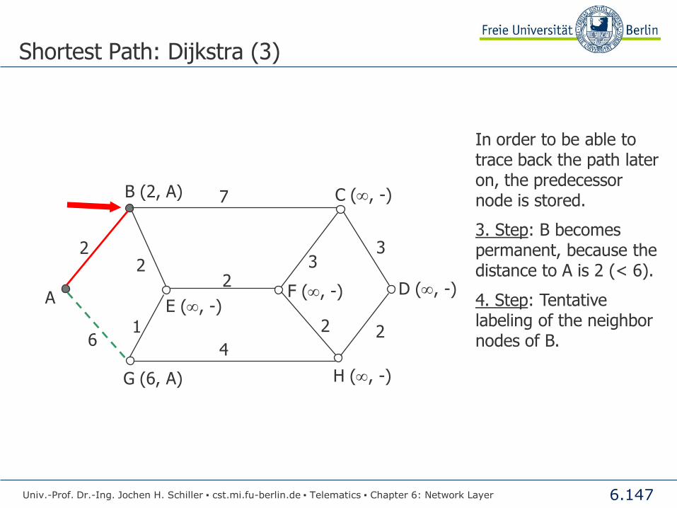
6.147

A

B (2, A)

E (, -)

G (6, A)

F (, -)

H (, -)

D (, -)

C (, -)

2 2

2

2 2 6 1

4

7

3 3

In order to be able to trace back the path later on, the predecessor node is stored.

3. Step: B becomes permanent, because the distance to A is 2 (< 6).

4. Step: Tentative labeling of the neighbor nodes of B.



6.148

A

B (2, A)

E (4, B)

G (6, A)

F (, -)

H (, -)

D (, -)

C (9, B)

E (4, B): Distance of A to E sums up to 4 using the path BE.

5. Step: E becomes permanent, since the distance to A is 4 (< 6 < 9).

6. Step: Tentative labeling of the neighbor nodes of E.

2 2

2

2 2 6

1

7

3 3

4



6.149

A

B (2, A)

E (4, B)

G (5, E)

F (6, E)

H (, -)

D (, -)

C (9, B)

5. Step: Preliminary label of G is over-written.

6. Step: G becomes permanent, since the distance to A is 5 (< 6 < 9).

7. Step: Tentative labeling of the neighbor nodes of G.

2 2

2

2 2 6

1

7

3 3

4



6.150

A

B (2, A)

E (4, B)

G (5, E)

F (6, E)

H (9, G)

D (, -)

C (9, B)

8. Step: Tentative label of G is overwritten.

9. Step: F becomes permanent, since the distance to A is 6 (< 9).

10. Step: Tentative labeling of the neighbor nodes of F.

2 2

2

2 2 6

1

7

3 3

4



6.151

A

B (2, A)

E (4, B)

G (5, E)

F (6, E)

H (8, F)

D (10, H)

C (9, B)

2 2

2

2 2 6 1

7

3 3

11. Step: H becomes permanent, since the

distance to A is 8 (< 9).

12. Step: Tentative labeling of the neighbor

nodes of H.

13. Step: C becomes permanent, since the distance to A is 9 (< 10).

4



6.152

A

B (2, A)

E (4, B)

G (5, E)

F (6, E)

H (8, F)

C (9, B)

D (10, H)

The distance to D using C is larger than the tentative label of D. No more paths exist, no states are changed - the algorithm terminates.

2 2

2

2 2 6

1

7

3 3

4



6.153

A

B (2, A)

E (4, B)

G (5, E)

F (6, E)

H (8, F)

C (9, B)

D (10, H)

2 2

2

2 2 6

1

7

3 3

14. Step: D is reached on the shortest path and finally becomes permanent.

4



6.154

Implementation of Dijkstra (1)

#define MAX_NODES 1024 /* maximum number of nodes */

#define INFINITY 1000000000 /* a number larger than every maximum path */

int n; int dist[MAX_NODES][MAX_NODES]; /* dist[i][j] is the distance from i to j */

void shortest_path(int s, int t, int path[])

{ /* s = source node, t = terminal node */ struct state { /* the path being worked on */

int predecessor; /* previous node */

int length; /* length from source to this node */

enum {permanent, tentative} label; /* label state */

} state[MAX_NODES];

int i, k, min;

struct state *p;

for (p = &state[0]; p < &state[n]; p++) { /* initialize state */

p->predecessor = -1;

p->length = INFINITY;

p->label = tentative;

}

state[t].length = 0;

state[t].label = permanent;

k = t; /* k is the initial working node */ /* The algorithm starts with the terminal node */ // Next Slide


6.155

Implementation of Dijkstra (2)

do { /* Is there a better path from k? */

for (i = 0; i < n; i++) /* this graph has n nodes */

if (dist[k][i] != 0 && state[i].label == tentative) {

if (state[k].length + dist[k][i] < state[i].length) {

state[i].predecessor = k;

state[i].length = state[k].length + dist[k][i];

}

}

/* Find the tentatively labeled node with the smallest label. */

k = 0;

min = INFINITY;

for (i = 0; i < n; i++)

if (state[i].label == tentative && state[i].length < min) {

min = state[i].length;

k = i;

}

state[k].label = permanent;

} while (k != s);

/* Copy the path into the output array. */

i = 0;

k = s;

do {

path[i++] = k;

k = state[k].predecessor;

} while (k >= 0);

}// shortest_path


6.156

Distance Vector Routing

Routing


6.157


● Problem: Static routing approaches are inflexible, they do not react to problems

● Solution: Routers mutually exchange (regularly) information about the current state of outgoing lines

● Distance Vector Routing

● Adaptive variant of shortest path routing

● Bellman et al. 1957

● Related names

● Distributed Bellmann-Ford Routing

● Ford-Fulkerson Routing

● RIP (ARPANET, Internet); improved in Cisco routers

● Properties of the Distance Vector

Routing

● Shortest-path routing

● Distributed

● Iterative

● Asynchronous

● Self-terminating


6.158


● The Distance Vector Routing

● Every router manages a table with (known/estimated) distances to each destination and the assigned lines to neighbor nodes

● Each router is assumed to know the distances to its neighbors

● Regularly, the distance information of the routing tables is communicated to the

neighbors

● Based on the information from the neighbors and the known distances to the

neighbors every router re-computes its routing table

● Without the use of the own old routing information

● Example of a Distance Vector: DVj = [(A=2), (B=3), (C=1), …]

● A is reachable with costs 2

● B is reachable with costs 3

● C is reachable with costs 1


6.159



Distance Vector Algorithm 1 Initialization:

2 for all destinations y in N:

3 Dx(y) = c(x,y) // if y is not a neighbor then c(x,y) = ∞

4 for each neighbor w

5 Dw(y) = ∞ for all destinations y in N

6 for each neighbor w

7 send distance vector DVx = [Dx(y): y in N] to w

8

9 Loop:

10 wait (until I see a link cost change to some neighbor w or

11 until I receive a distance vector from some neighbor w)

12

13 for each y in N:

14 Dx(y) = minv{c(x,v)+Dv(y)}

15

16 if Dx(y) changed for any destination y

17 send distance vector DVx = [Dx(y): y in N] to all neighbors

Terms

● c(x,y) Cost of link (x,y)

● Dx(y) Distance from node x to y

● DVx Distance vector of node x

6.160

Distance Vector Routing: Information Exchange

Essential here:

Global information is exchanged only between neighbors!

Estimation of J for its neighbors JA = 8, JI = 10, JH = 12, JK = 6


8 12

10 6

6.161

Table of router A after system

initialization or “cold start”

Table of router B after system

initialization or “cold start”

As “transmission costs” for each line, 1 is assumed.

Distance Vector Routing: Example


From A to Link Costs

A Locally 0

From B to Link Costs

B Locally 0

A L1 L2

L3 L4

L5

L6

B C

D E

6.162


● A transfers (A=0) to its

neighbors B and D.

● B and D know from where the

vector comes and so the costs to A

can be computed.

● Routing tables of routers B and D, after the vector of router A is

processed.



B Locally 0

A L1 1

From D to Link Costs

D Locally 0

A L3 1

A L1 L2

L3 L4

L5

L6

B C

D E

6.163

Routing table of A after updating with information coming from D and B

B now transfers its vector (B=0, A=1) using link L1, L2, and L4 to its neighbors A, C, and E.

A receives this vector over link L1 and updates its table as follows:

A=2 is larger than A=0 discard B=1 for link L1

Similar to this, the vector of D is processed.




A Locally 0

B L1 1

D L3 1

A L1 L2

L3 L4

L5

L6

B C

D E

6.164

Router C receives (B=0, A=1)

Router E receives (B=0, A=1)



From C to Link Costs

C Locally 0

B L2 1

A L2 2

From E to Link Costs

E Locally 0

B L4 1

A L4 2

A L1 L2

L3 L4

L5

L6

B C

D E

6.165

Router E receives the vector (D=0, A=1) which it uses to update the routing table with D=1 and A=2 using link L6. The entry for A over link L4 is already registered with costs of 2, therefore no new entry for A is necessary.

Routing table of E after the update. A, C, and E now have new routing tables. generate distance vectors




E Locally 0

B L4 1

A L4 2

D L6 1

A L1 L2

L3 L4

L5

L6

B C

D E

6.166

From A: (A=0, B=1, D=1) over link L1 and L3.

From C: (C=0, B=1, A=2) over link L2 and L5.

From E: (E=0, B=1, A=2, D=1) over link L4, L5, and L6. Routing table of B:




B Locally 0

A L1 1

D L1 2

C L2 1

E L4 1

A L1 L2

L3 L4

L5

L6

B C

D E

6.167

From A: (A=0, B=1, D=1) over link L1 and L3.

From C: (C=0, B=1, A=2) over link L2 and L5.

From E: (E=0, B=1, A=2, D=1) over link L4, L5, and L6.




D Locally 0

A L3 1

B L3 2

E L6 1


E Locally 0

B L4 1

A L4 2

D L6 1

C L5 1

A L1 L2

L3 L4

L5

L6

B C

D E

6.168

From B: (B=0, A=1, D=1, C=1, E=1) over link L1, L3, and L4.

From D: (D=0, A=1, B=2, E=1) over link L3 and L6.

From E: (E=0, B=1, A=2, D=1, C=1) over link L4, L5, and L6.




A Locally 0

B L1 1

D L3 1

C L1 2

E L1 2


C Locally 0

B L2 1

A L2 2

E L5 1

D L5 2

A L1 L2

L3 L4

L5

L6

B C

D E

6.169

From B: (B=0, A=1, D=1, C=1, E=1) over link L1, L3, and L4.

From D: (D=0, A=1, B=2, E=1) over link L3 and L6.

From E: (E=0, B=1, A=2, D=1, C=1) over link L4, L5, and L6.

The algorithm terminates since A, C, and D create and send new vectors, but B, D, and E do not have to apply updates any longer.




D Locally 0

A L3 1

B L3 2

E L6 1

C L6 2

A L1 L2

L3 L4

L5

L6

B C

D E

6.170

Distance Vector Routing: Successive Information Propagation

● Problem with this procedure: Information must be reliable

● Otherwise: Christmas Deadlock

● A router j announced DVj = (0, …, 0)

● Consequence: Nearly the entire traffic was led over j

● Result: Collapse

● Disadvantages:

● Unreliable information is dangerous

● Cycling load conditions

● Additional overhead

● And: information propagation lasts a certain time!


6.171

Router A and B notice the interruption, e.g. by control packets. Update of their own routing tables

Inf = Infinite

Distance Vector Routing: Connection Loss



A Locally 0

B L1 Inf

D L3 1

C L1 Inf

E L1 Inf


B Locally 0

A L1 Inf

D L1 Inf

C L2 1

E L4 1

A L1 L2

L3 L4

L5

L6

B C

D E

6.172

From A: (A=0, B=inf, D=1, C=inf, E=inf) over link L3

From B: (B=0, A=inf, D=inf, C=1, E=1) over link L2 and L4

D receives the vector from A and updates with A=1, B=inf, D=2, C=inf, E=inf




D Locally 0

A L3 1

B L3 Inf

E L6 1

C L6 2

A L1 L2

L3 L4

L5

L6

B C

D E

6.173

From A: (A=0, B=inf, D=1, C=inf, E=inf) over link L3

From B: (B=0, A=inf, D=inf, C=1, E=1) over link L2 und L4




C Locally 0

B L2 1

A L2 Inf

E L5 1

D L5 2


E Locally 0

B L4 1

A L4 Inf

D L6 1

C L5 1

A L1 L2

L3 L4

L5

L6

B C

D E

6.174

From D: (D=0, A=1, B=inf, E=1, C=2) over link L3 and L6

From C: (C=0, B=1, A=inf, E=1, D=2) over link L2 and L5

From E: (E=0, B=1, A=inf, D=1, C=1) over link L4, L5, and L6




A Locally 0

B L1 Inf

D L3 1

C L3 3

E L3 2


B Locally 0

A L1 Inf

D L4 2

C L2 1

E L4 1

A L1 L2

L3 L4

L5

L6

B C

D E

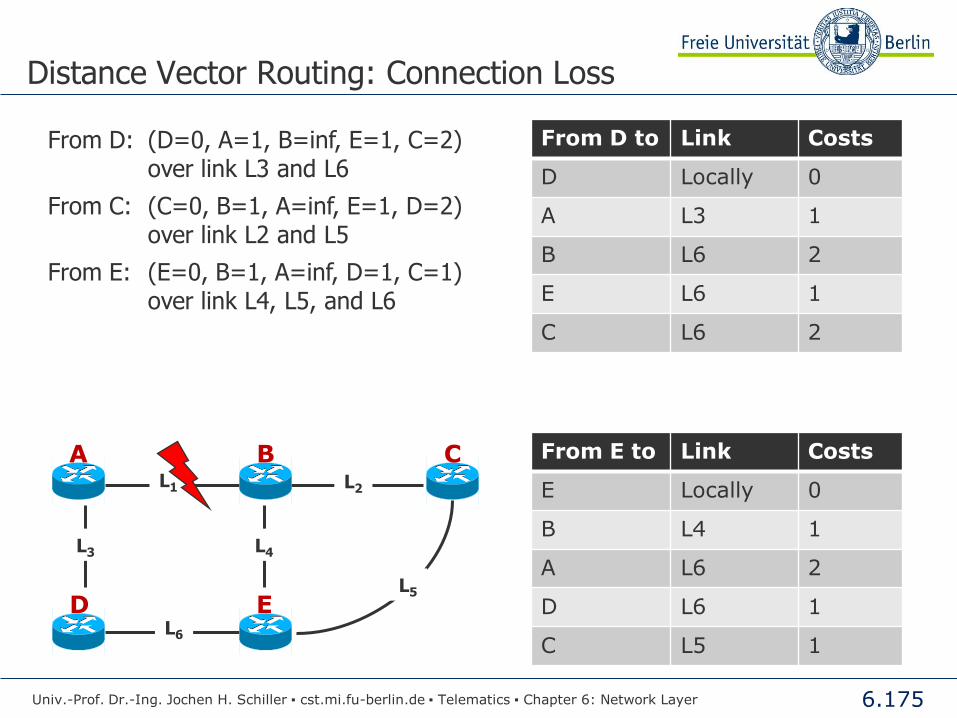
6.175

From D: (D=0, A=1, B=inf, E=1, C=2) over link L3 and L6

From C: (C=0, B=1, A=inf, E=1, D=2) over link L2 and L5

From E: (E=0, B=1, A=inf, D=1, C=1) over link L4, L5, and L6




D Locally 0

A L3 1

B L6 2

E L6 1

C L6 2


E Locally 0

B L4 1

A L6 2

D L6 1

C L5 1

A L1 L2

L3 L4

L5

L6

B C

D E

6.176

From A: (A=0, B=inf, D=1, C=3, E=2) over link L3

From B: (B=0, A=inf, D=2, C=1, D=1) over link L2 and L4

From D: (D=0, A=1, B=2, E=1, C=2) over link L3 and L6

From E: (E=0, B=1, A=2, D=1, C=1) over link L4, L5, and L6




A Locally 0

B L3 3

D L3 1

C L3 3

E L3 2


B Locally 0

A L4 3

D L4 2

C L2 1

E L4 1

A L1 L2

L3 L4

L5

L6

B C

D E

6.177

From A: (A=0, B=inf, D=1, C=3, E=2) over link L3

From B: (B=0, A=inf, D=2, C=1, D=1) over link L2 and L4

From D: (D=0, A=1, B=2, E=1, C=2) over link L3 and L6

From E: (E=0, B=1, A=2, D=1, C=1) over link L4, L5, and L6

The algorithm terminates, because A, B, and C create and send new vectors, but do not cause further updates in the routing tables.




C Locally 0

B L2 1

A L5 3

E L5 1

D L5 2

A L1 L2

L3 L4

L5

L6

B C

D E

6.178

So far: Costs of 1 for each link

Reality: Different costs per link

Example: Link L5 has costs of 10

In the following, only the paths to router C are examined.

In the case of stable conditions the tables of the other routers have these entries for C.

Distance Vector Routing: The Bouncing Effect


From Link Costs

A to C L1 2

B to C L2 1

C to C Locally 0

D to C L3 3

E to C L4 2

A L1 L2

L3 L4

L5

L6

B C

D E

1 1

1

1

1

10

6.179


● Assumption 1: Connection 2

breaks down.

● B detects the failure and sets

its costs to inf.

● Temporarily, the following

table results:

● Assumption 2: A has sent its

vector before B.

● in case of regular transmission this may happen often


From Link Costs

A to C L1 2

B to C L2 Inf

C to C Locally 0

D to C L3 3

E to C L4 2

A L1 L2

L3 L4

L5

L6

B C

D E

1 1

1

1

1

10

6.180


● A reports C over link L1 with costs

of 2

● Router B adds costs of 1 to link L1

for C

● Value is lower than inf

● Table entry for C is replaced by link

L1 and costs of 3

● Passing on the table to A and E

● Message comes over link L1 resp.

4, which A and E are using for C

● Update of A and E


From Link Costs

A to C L1 4

B to C L1 3

C to C Locally 0

D to C L3 3

E to C L4 4

A L1 L2

L3 L4

L5

L6

B C

D E

1 1

1

1

1

10

6.181


● Routing tables contain a loop!

● Packets from C are bouncing

between A and B

● C sends its vector over link L5

● E adds costs of 10 to its own costs of 0

● E ignores the message, because the

costs are higher as before

● A and E send vectors

● Update of B and D


From Link Costs

A to C L1 4

B to C L1 5

C to C Locally 0

D to C L3 5

E to C L4 4

A L1 L2

L3 L4

L5

L6

B C

D E

1 1

1

1

1

10

6.182


● After several iterations, the

following table results:

● Entries depend however on

random processes (e.g. on the

order of the update messages,

the arrival times of the vectors,

losses of vectors etc.)


From Link Costs

A to C L1 12

B to C L4 11

C to C Locally 0

D to C L6 11

E to C L5 10

6.183

A B C D E 1 1 1 1

Distance Vector Routing: Count to Infinity

● Count to Infinity problem:

● The Distance Vector Routing achieves a correct solution, but possibly many (up to infinite) update steps are necessary.

● Example:

● Five routers A, B, C, D, and E are connected in a linear fashion, the distance

between neighbor routers in each case is 1.


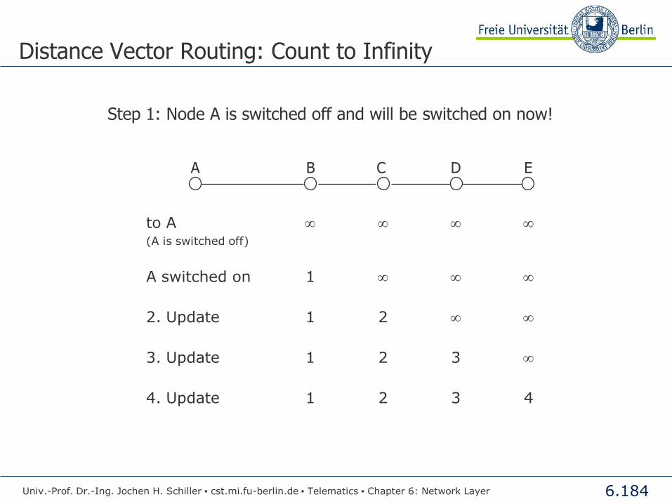
6.184

Step 1: Node A is switched off and will be switched on now!


to A (A is switched off)

1 A switched on

2 1 2. Update

3 2 1 3. Update

4 3 2 1 4. Update

A B C D E


6.185

6 5 6 5 4. Update

4 3 2 1 A switched off

4 3 2 3 1. Update

4 3 4 3 2. Update

4 5 4 5 3. Update

8 7 8 7 6. Update

Step 2: A is switched off


A B C D E

: :

: :

: :

: :


6.186

A B

C

D

Distance Vector Routing: Split Horizon Algorithm

● First solution: Split-Horizon Algorithm

● Do not send the distance to X over that link

used to transfer packets for X (resp. path is

reported as infinity).

● However, it does not work always:

● Link CD is switched off

● C hears from A and B that they do not reach D

● C announces A and B that D is unreachable

● B announces however to A: D has distance 2

● A updates and has D with distance 3

● B updates for D with distance 4 ......

● Count to Infinity

Router


6.187

Routing Information Protocol (RIP)

Routing


6.188

Routing Information Protocol (RIP)

● Routing Information Protocol (RIP, RFC 1058) ● Early internal gateway routing

protocol used in the Internet

● Based on the Distance Vector Protocol

● RIP messages are sent every 30 seconds as UDP datagrams

● Used metric for the evaluation of the paths is the number of hops ● The maximum number of hops is

limited to 15 16 = ∞

● In a message (only) up to 25 entries of the routing table can be sent

● Fits good for small systems

● Problems: ● Slow convergence (duration of

minutes)

● Count to Infinity

● No considering of subnets

● RIPv2 (RFC 2453): ● Subnets, CIDR

● Authentication

● Multicast, etc.

● However: max. number of hops is still limited to 15

● RIPng (RFC 2080) ● IPv6 support

● Internet Gateway Routing Protocol (IGRP) ● As reaction to the restrictions of RIP

Cisco introduced IGRP

● Extension of the metric, load sharing, more efficient packet format

● The protocols did not become generally accepted, because they were Cisco specific

● Replaced by EIGRP (new design)

● Replacement by a Link State Protocol (OSPF)


6.189

1.) Exchange of global information locally (only with neighbors)


2.) Global exchange of local information

Link State Routing

Routers exchange Link State Advertisements (LSA)

Information Exchange


6.190

Link State Routing

Routing


6.191

Link State Routing

● Every router

● determines its neighbors and their addresses

● HELLO packets

● measures the distances to the neighbors

● ECHO packets

● sends these information in a packet to all other routers

● Link State Advertisement (LSA)

● computes on the basis of all the received LSAs from other routers the shortest

paths to the other routers (e.g. with the Dijkstra algorithm)

● This is repeated regularly.


6.192

A

B

C

D E

F

G

H

I

LAN

A

B

C

D E

F

G H

I

N

Link State Routing

● First step:

● Determination of all neighbor routers

● Sending of a HELLO message on all

links

● Routers at the other-end answer with

their identification

● If several routers are connected in a

(broadcast) network, a

new “artificial” node

is introduced for simplification


6.193

A

B C

D

E

F

G

H

I J

Link State Routing

● Second step: Discovery of link

costs

● Transmission of ECHO messages

● Routers at the other end answer

immediately (measurement of the

delay)

● Inclusion of load leads to the choice of the lowest loaded link

● Side-effect in having two possible

links: the less loaded link is loaded

immediately heavily and the other link becomes free, with the next

measurement the same happens for the other link, … (cycling load)


Cycling between both links, because of changing load!

6.194

Link State Routing

● Third step: Create link state messages

● Contains list of neighbors with appropriate “link costs” (Delay, queue length, jitter, etc.)

● Messages additionally contain sender

identification, sequence number, and age.

A

B C

D

E F

5

1

2

4

6

7

8

3


A

Seq.No.

Age

B 4

E 5

B

Seq.No.

Age

A 4

C 2

F 6

C

Seq.No.

Age

B 2

D 3

E 1

D

Seq.No.

Age

C 3

F 7

E

Seq.No.

Age

A 5

C 1

F 8

F

Seq.No.

Age

B 6

D 7

E 8

6.195

A

F

E

C

D

21

21

21

20

21

60

60

59

60

59

0

1

0

1

1

1

1

1

0

0

1

0

0

1

0

1

0

1

0

0

0

0

0

1

1

0

1

1

0

1

Source Seq.No. Age A C A F F C

Transmission flags Confirmation flags

Data

Packet Buffer for Router B

● Fourth step: Sending of link state messages

● Flooding (problem: loops, duplicates, packet losses, etc.)

● Sequence numbers are counted up, packets with outdated numbers (duplicates)

are discarded

● Every router reduces the “age” by one, with zero a packet is discarded

● Each router confirms

the arrival of a link

state packet to

the sending router

Data structure of router B • Flags are for the

lines of router B


6.196

A

F

E

C

D

21

21

21

20

21

60

60

59

60

59

0

1

0

1

1

1

1

1

0

0

1

0

0

1

0

1

0

1

0

0

0

0

0

1

1

0

1

1

0

1

Source Seq.No. Age A C A F F C

Transmission flags Confirmation flags

Data

Packet Buffer for Router B

● Link state message from A arrives directly, therefore Age=60, Seq.No.=21

● Message is sent to C and F, and confirmed for A

● Message of F must be forwarded to A and C,

and be confirmed for F

● Message of E came twice (over EAB and EFB)

therefore only

forwarding to C,

confirmation for A and F

A

B C

D

E F 5

1

2 4

6 7

8

3


6.197

Route Enquiry

● Fifth step: Decision on best routes

● Router collects link state information from all other routers

● A path graph for the entire sub-network is determined

● Local execution of e.g. the Dijkstra algorithm for the determination of the

optimal route

● Results are written into the routing table

● Problems:

● With n routers and m neighbors, nm table entries are necessary

● In the case of router failures, the graphs of all routers are outdated

● Extremely susceptibly to attacks


6.198

Hierarchical Routing

Routing


6.199

Routing Tables

● Problem: extensive routing tables

hierarchical routing

● Large tables require too much memory, CPU time, transmission capacity

for link state messages, etc.

virtual division of the network (Regions)


6.200

1A 1C

1B 2A

2C

2B

2D

5C

5D 5E

4B

5B

5A 4C

4A 3A

3B

Region 1

Region 5 Region 4

Region 2

Region 3



6.201

1A

1C

1B 2A

2C

2B

2D

5C

5D 5E

4B

5B

5A 4C

4A 3A

3B

Region 1

Region 5 Region 4

Region 2

Region 3

Disadvantage: Possibly increasing path length



Full routing table for 1A

Dest. Link to Hops

1A - -

1B 1B 1

1C 1C 1

2A 1B 2

2B 1B 3

2C 1B 3

2D 1B 4

3A 1C 3

3B 1C 2

4A 1C 3

4B 1C 4

4C 1C 4

5A 1C 4

5B 1C 5

5C 1B 5

5D 1C 6

5E 1C 5

Hierarchical routing table for 1A

Dest. Link to Hops

1A - -

1B 1B 1

1C 1C 1

2 1B 2

3 1C 2

4 1C 3

5 1C 4

6.202

Open Shortest Path First (OSPF) Intermediate System to Intermediate System (IS-IS)

Routing / Interior


6.203

Open Shortest Path First (OSPF)


● 1990 standardized by IETF (RFC 1247)

● Current versions:

● OSPF version 2 (RFC 2328) for IPv4

● OSPF version 3 (RFC 5340) with IPv6 support

● Open protocol (not manufacturer specific)

● Supports a multiplicity of metrics (distance, delay, etc.)

● Dynamic algorithm for fast adjustment to changing conditions in the network

● Load sharing between redundant links

● Supports hierarchical systems

● Contains security mechanisms to protect routers from wrong routing information

or attacks

● Three types of connections are supported:

● Point-to-point links between routers

● Broadcast networks (mostly LANs)

● Multi-access networks without broadcasting (e.g. packet switching WANs)


6.204


● Autonomous Systems (AS)

● The Internet is divided into autonomous systems (AS)

● Each autonomous system has a backbone, which connects all parts of the AS

● Large autonomous systems are divided into areas

● Area of an AS

● Within an area every router has the same link state database and implements

the same algorithm for determination of the shortest path

● Every router, which belongs to two or more areas, is part of the backbone

● A router, which connects two areas, needs the link state databases from both

areas


6.205


● OSPF distinguishes four router classes

● For reducing the extent of routing tables

● Classes of routers

● Internal routers, which only belong to one area

● Area routers at the border of areas, which connect two or more areas

● Backbone routers, which are placed at the backbone

● AS border routers, which mediate between several autonomous systems


6.206

Area router

External protocols connect the autonomous systems

Backbone

Backbone router

Area

Internal router

Border router of the autonomous system

AS 1 AS 2

AS 3 AS 4

Relationship between autonomous systems, backbones, and areas in OSPF



6.207

Intermediate System to Intermediate System (IS-IS)

● Standardized in the context of OSI for the connectionless layer 3 protocol

● Republished by IETF as RFC 1142 (however sometimes also cited as IS-IS=0 …)

● Link-state, very similar to OSPF, based on Dijkstra

● Neutral to layer 3 protocol (OSPF routes IP, originally v4)

● Thus IPv6 got faster support by IS-IS

● Routers also build a map of the network, calculate shortest path

● Lower overhead compared to OSPF, better scalability

● Often used by network operators with many routers


6.208

Border Gateway Protocol (BGP)

Routing / Exterior


6.209


● Goal difference between internal and external protocols

● Interior gateway protocols are designed for efficiency

● Find the best way to the destination host

● Exterior gateway protocols have to consider policies

● Political, economical, …


● BGPv4 (RFC 4271, RFC 4274, RFC 4276)

● De-facto standard inter-AS routing protocol in the Internet

● An external routing protocol

● Variant of the Distance Vector Protocol: not the costs of a transmission path are

being monitored and exchanged, but the complete description of paths (Path Vector Protocol)

● Considers security and other rules (Routing Policies)

● Communicates the neighbor routers the whole path which is to be used (deterministically)

● Uses TCP for data exchange (port 179)


6.210

Information sent to F F receives the following information about D from its neighbors: from B: “I use BCD” from G: “I use GCD” from I: “I use IFGCD” from E: “I use EFGCD”

Assumption: F uses FGCD to reach D

F searches for the optimal route

● Paths of I and E are directly discarded, because they cross F

● B and G are possible options

● Application of Policies

● Routes, which violate policies, are being set to infinity

H

A

C B

G

F

E

D

J I



BGP Example: Dest. Net. Next-Hop Path … (see RFC 4271)

141.3.0.0/16 195.221.222.254 5409 1275 553

6.211

Size of BGP routing tables (bgp.potaroo.net)


6.212

Number of unique Ass (bgp.potaroo.net)


6.213

Average AS path length


6.214

BGP is crucial to the Internet

● Many issues / problems

● Stability, routing table growth, load balancing in multi-homed networks, hijacking …

● Suggested reading

● Delayed Internet Routing Convergence

● 2-year measurements of BGP convergence

● It takes between 3 and 15 minutes for paths to converge

● http://conferences.sigcomm.org/sigcomm/2000/conf/paper/sigcomm2000-5-2.pdf

● Analysis of BGP Update Burst during Slammer Attack

● Consequences of the slammer worm on BGP in 2003

● Shows nicely the effect of small ASs on the global update traffic

- Two small ASs that contribute only to 0.25% of routing table entries caused 6% of all BGP update messages

● http://irl.cs.ucla.edu/papers/mohit_iwdc03.pdf

● Measurement of Highly Active Prefixes in BGP

● Examines the stability of routes and shows that very few prefixes contribute to the majority of BGP update traffic

● http://www.cs.ucla.edu/~lixia/papers/05Globcom.pdf


http://conferences.sigcomm.org/sigcomm/2000/conf/paper/sigcomm2000-5-2.pdf






http://irl.cs.ucla.edu/papers/mohit_iwdc03.pdf

http://www.cs.ucla.edu/~lixia/papers/05Globcom.pdf

6.215

Summary

● TCP/IP reference model defines only one protocol for layer 3

● The Internet Protocol (IP)

● Connectionless transmission, data packets are forwarded hop-by-hop

● Supported by routing protocols to determine the best way to a destination

● ICMP for exchange of control messages

● ARP for mapping of IP addresses to MAC addresses

● But, there are several problems with the “current” IPv4

● address space, security, mobility, quality of service, …

● Large number of additional protocols to deal with these problems: network

address translation, IPsec, Mobile IP, IntServ, DiffServ, MPLS, …

● Successor IPv6 could deal with (some of) the problems, but

when/where/to what extend will it come?

● See e.g. http://resources.potaroo.net/iso3166/v6cc.html for current usage


http://resources.potaroo.net/iso3166/v6cc.html

http://resources.potaroo.net/iso3166/v6cc.html

telematics chapter 6: network layer - freie universität · · 2012-09-03telematics chapter 6:...

Documents