Another look at P/E ratios

February, 2006

by

Jacob K. Thomas†

(jacob.thomas@yale.edu) and

Huai Zhang§ (hzhang@business.hku.hk)

† Yale School of Management, New Haven, CT, 06520. § School of Business, University of Hong Kong, Pokfulam, Hong Kong We thank two anonymous referees, Peter Easton, Alistair Hunt, Terry Shevlin, K.R. Subramanyam and workshop participants at University of Southern California and the University of Utah (Annual Winter Accounting Workshop) for helpful comments and the Faculty Research Fund of Columbia Business School for financial support.

Preliminary. Comments welcome.

Another look at P/E ratios

Abstract

Price-earnings (P/E) ratios should be positively related to growth and negatively related to

interest rates and risk. Whereas earlier investigations of the determinants of P/E ratios find these

links to be weak, results of recent research estimating the cost of capital imply stronger links.

The two sets of research employ different sets of proxies for P/E ratios (trailing vs. forward

ratios), growth (observed vs. forecast growth) and risk. We update the literature investigating the

determinants of P/E ratios by contrasting the results based on the two sets of proxies. We also

investigate a recent finding which suggests that forward P/E ratios are negatively related to the

volatility of reported earnings, even though reported earnings volatility does not appear in the

relation derived for forward P/E ratios. Our results suggest an indirect connection: firms with

lower earnings volatility, due to lower cash flow volatility and greater earnings smoothing due to

accruals, are associated with higher growth prospects and lower risk.

1

Another look at P/E ratios

I. Introduction

Both intuitive (e.g., Gordon, 1962) and formal (e.g., Fairfield, 1994) analyses of the

factors that determine price-earnings (P/E) ratios predict a positive relation with anticipated

growth and a negative relation with expected rates of return, which in turn implies a negative

relation with risk and nominal interest rates. Prior empirical efforts to explain variation in P/E

ratios (e.g., Beaver and Morse, 1978 and Penman, 1996) have, however, uncovered only weak

relations between P/E ratios and risk/growth, especially at the firm level. However, recent work

on estimating the cost of equity (e.g., Easton, 2004) suggests that P/E ratios are related to

growth, and the implied cost of equity based on those P/E ratios and growth forecasts is related

to risk. One difference between the two sets of studies is the use of analyst forecast data: in

recent research P/E ratios are based on forward rather than trailing earnings, and growth is based

on forecast rather than observed earnings growth. Another difference is the use of additional

measures of risk (e.g., market capitalization and P/B ratio), beyond the betas used in earlier

research. Our objective is to update the research on the determinants of P/E ratios by

investigating the improvement due to these newer measures. A related but more ambitious

objective is to expand the list of factors that impact P/E ratios beyond those predicted by theory

to include the volatility of reported earnings, since some recent research (e.g., Barth et al., 1999)

suggests that smoother earnings enjoy higher valuations. Given the practical bent of this line of

research, we focus on simple linear relations based on available proxies.

To understand the impact of interest rates on P/E ratios, we calculate aggregate forward

and trailing E/P ratios (by summing up earnings and prices across all firms in the cross-section)

and compare the time-series of those earnings yields against long-term risk-free rates (proxied by

10-year Treasury bond yields). We confirm the results first reported in the popular “Fed

Valuation Model” (Greenspan, 1997), which indicate a strong negative link between forward P/E

ratios and prevailing long-term interest rates. We find that the corresponding comovement with

trailing P/E ratios is also evident, but not as strong. When reporting results for trailing P/E ratios,

2

we consider trailing earnings before extraordinary items and discontinued operations as reported

by the firm (referred to as Compustat EPS) as well as trailing earnings as reported by IBES

(referred to as IBES EPS). The latter measure excludes many but not all one-time components

included in the former.1 The observed negative comovement with interest rates is more evident

for IBES EPS, relative to the comovement observed for Compustat EPS, probably because IBES

EPS contains fewer one-time items.

Turning to firm-level determinants of P/E ratios, we begin by regressing E/P ratios on

interest rates, observed future growth and two traditional measures of risk, market model betas

and standard deviation of returns. Contrary to theory and intuition, we find that P/E ratios are

positively related to risk, and the link with observed growth is positive, but only weakly so.

(Although our analyses are estimated on E/P ratios, we prefer to describe our results in terms of

P/E ratios.) However, switching the growth measure from observed growth to forecast growth

reverses the association for risk and improves dramatically the positive relation with growth.

Apparently, observed growth measures anticipated growth with error that is systematically

biased, and that measurement error is correlated with risk. Unlike the dramatic improvement

observed when past growth is replaced by forecast growth, introducing newer measures of risk

(market capitalization and the P/B ratio) does not change the overall tenor of the results. Finally,

even though aggregate trailing P/E ratios are negatively related to interest rates, at the firm level

that relation is unexpectedly positive. Switching to forward P/E ratios reverses that firm-level

relation to the positive comovement with interest rates predicted by theory.

Our second investigation, which represents a substantial fraction of our efforts to update

research on the determinants of P/E ratios, concerns the potential link between P/E ratios and

volatility of reported earnings. Even though the relations derived for P/E ratios do not indicate a 1 IBES EPS, or the “Actual” EPS provided by IBES, is intended to capture the portion of reported EPS that was

being forecast by a majority of analysts. To the extent that analysts focus on “core” or “recurring” EPS, they do not forecast many one-time components of reported EPS and those components are excluded from IBES EPS. However, analysts forecast some one-time components if they are deemed to be value-relevant. For example, Gu and Chen (2004) provide a comprehensive survey of the treatment of non-recurring items in forecast and actual eps for First Call data. They consider different types of non-recurring items (Table 4), and report that 4028 forecasts among a sample of 28,542 analysts’ forecasts (14.11%) contain nonrecurring items.

3

direct role for reported earnings volatility, the popular financial press has long suggested that

managers make discretionary accruals to smooth reported earnings, and the rationale typically

offered is that smoothed earnings are rewarded with higher valuations (e.g., Smith et al., 1994).

The academic literature too has recently accumulated evidence that suggests that smoothed

earnings are associated with higher valuations (e.g. Barth et al., 1999). Note two differences that

separate our paper from that literature (a more detailed discussion is provided in the paragraphs

that follow). First, prior research focuses mainly on managerial efforts to smooth reported

earnings via discretionary accruals, whereas we are concerned more broadly with the volatility of

reported earnings. Second, the impact of smoothing reported earnings on valuations per dollar of

earnings is estimated differently: while prior research investigates the impact of variation across

different levels of earnings smoothing on the coefficient on earnings in a regression of price on

earnings, we regress E/P ratios on volatility of reported earnings.

To understand the first difference—overall volatility of reported earnings versus the

reduction in that volatility due to nondiscretionary accruals alone—we use the description

provided in Hunt et al. (2000). Each firm is associated with an inherent volatility, proxied by the

time-series volatility of cash flows from operations. The accrual process, as determined by

applicable GAAP, then adds non-discretionary accruals to generate non-discretionary or

unmanaged earnings. In general, these non-discretionary accruals cause unmanaged earnings to

exhibit lower volatility than cash flows. Finally, managers wishing to smooth out spikes in

unmanaged earnings add discretionary accruals to provide an even smoother series for reported

earnings. The volatility of reported earnings can thus be viewed as due to three components:

volatility of cash flows, reduction in earnings volatility due to nondiscretionary accruals, and a

potential for further reduction in earnings volatility due to discretionary accruals. We combine

the second and third components, because of concerns about our ability to separate discretionary

and nondiscretionary accruals (details discussed later), and consider how the volatility of cash

flows and the reduction in earnings volatility due to total accruals impact P/E ratios.

4

The second difference—choice between estimating regressions of price on reported

earnings versus E/P ratios on earnings volatility—is determined by the importance assigned to

measurement error. Smoothing reported earnings has two potential effects on the coefficient on

earnings in a valuation regression: a) it results in a higher valuation per dollar of reported

earnings because smoother earnings are valued more highly by the market, and b) by reducing

the measurement error between reported and value-relevant permanent earnings, smoothing

increases the coefficient on earnings (e.g., Subramanyam, 1996). While the impact of this second

reason is an important research question, it has already been investigated by others. To focus our

investigation on the first reason, we estimate regressions of E/P on reported earnings volatility.

The extent to which our earnings proxy measures value-relevant permanent earnings with error is

now included in the regression error, and should not affect estimated coefficients.

To determine whether cash flow volatility and smoothing due to accruals (discretionary

and non-discretionary combined) are associated with higher valuations per dollar of forecast

earnings, we regress E/P ratios on both the volatility of reported earnings and the volatility of

cash flows from operations. While the coefficient on cash flow volatility describes the cash flow

effect, the coefficient on reported earnings volatility measures the effect of earnings smoothing

due to accruals (since that coefficient in a multiple regression indicates the separate effect of

reported earnings volatility after controlling for cash flow volatility). Our results suggest that

lower cash flow volatility and greater earnings smoothing due to accruals are both strongly

associated with higher P/E ratios.

Our final analysis seeks to determine whether reduced earnings volatility (due to

discretionary and nondiscretionary accruals) separately affects P/E ratios, beyond any indirect

effect caused by firms with lower earnings volatility also being associated with higher growth

and lower risk. Observing a separate effect creates a puzzle, since theory does not indicate a role

for cash flow volatility or smoothing due to accruals. While including proxies for growth and

risk to the regressions of E/P ratios on the two volatility measures decreases substantially the

coefficients on the volatility measures, a significant separate effect remains (especially for cash

5

flow volatility). We believe, however, that this observed residual relation between E/P ratios and

the two volatility measures is because our risk and growth proxies do not completely capture the

impact of risk and growth. If so, the underlying strong relations between the two volatility

measures and risk/growth capture any residual impact of risk and growth on P/E ratios.

To be sure, there are other explanations for our results based on market inefficiency for

why lower cash flow and earnings volatility result in higher P/E ratios. For example, firms that

smooth reported earnings might cause investors to underestimate the true risk or overestimate the

true growth associated with those firms, which in turn would also result in higher P/E ratios.

Although we do not investigate this possibility, the results in Hunt et al. (2000) suggest that

future indicators for firms with smoother earnings confirm that the higher valuations assigned to

these firms are justified. Also, our own efforts to build trading rules based on measures of

earnings smoothing did not suggest systematic overpricing for firms with smoother earnings

(results not reported here).

The rest of this paper is laid out as follows. The next section surveys the relevant prior

literature and Section III describes the derivation of the forward P/E ratio valuation equation and

develops our regression models. Section IV covers sample formation and variable definitions.

Section V describes the results and Section VI concludes the paper.

II. Prior research

Risk and growth as determinants of variation in P/E ratios

An early paper by Beaver and Morse (1978) considered the behavior of portfolios formed

on trailing E/P over the period between 1956 and 1974. Although they found that E/P ratios

persisted over time, observed long-term growth and risk measures explained little variation in

E/P, even at the portfolio level. They conclude that the persistent E/P differences are likely due

to persistent differences in accounting methods and estimates, rather than differences in growth

and risk. Zarowin (1990) examines a smaller sample of 175 large firms with analyst forecast data

over the 1961 to 1969 period and concludes that replacing forecasted long-term growth for

6

observed long-term growth alters the Beaver and Morse conclusions: cross-sectional variation in

portfolio-level trailing E/P is indeed significantly linked to forecasted long-term growth in

earnings.

More recently, Fairfield (1994) and Penman (1996) reconsider the determinants of P/E

(and P/B) ratios based on the residual income valuation model (Preinreich, 1938), described

below as equation (1). Fairfield (1994) derives a general relation for trailing E/P ratios that is laid

out below as equation (2).

( ) ( )...

11 221

00 ++

++

+=r

rir

ribvp (1)

( )( ) ( ) ⎥

⎦

⎤⎢⎣

⎡+

+∆

++

∆+

+=

+ ...11

112

0

2

0

1

0

00

keri

keri

kk

edp (2)

where p0= current price, bvt= book value at the end of year t (reported value for year 0 and forecast for future years), et=earnings for year t (reported value for year 0 and forecast for future years), k=equity discount rate or cost of equity, rit= residual income expected for year t, equal to et−k*bvt-1 d0=dividends for current year, ∆rit = rit − rit-1 is the change in expected residual income between years t and t-1.

The relation in equation (2) confirms the intuitive links between P/E ratios and

risk/growth that have been derived from the Gordon (1962) dividend growth model: P/E ratios

are positively related to growth and negatively related to equity discount rates. Equation (2)

improves on those intuitive links by providing clarification on how those measures should be

calculated. First, the P/E ratio should be calculated cum dividend (p0+d0), not ex dividend.

Second, the growth should be measured not as growth in dividends or earnings, but as growth in

residual income. Finally, that growth in residual income is scaled by current earnings (e0) and

discounted.

Penman (1996) reexamines the Beaver and Morse (1978) conclusion regarding the low

correlation between P/E ratios and observed long-term growth and finds a stronger relation using

a more recent sample period (1968-1985) and a measure of earnings growth that corrects for

7

dividends paid. Whereas the correlation between portfolio-level P/E ratios and observed growth

in Beaver and Morse (1978) declines substantially after the second year, Penman’s results show

higher correlations even nine years later. (Penman, 1996, does not provide follow-up analyses to

identify reasons for these observed differences in results.)

In sum, the research described above provides only weak empirical confirmation of the

predicted relations. While there is some evidence of a positive relation between P/E ratios and

growth, that relation is noted primarily at the portfolio level. Dropping down to the firm level

reveals substantially weaker relations. For example, in Penman (1996) the correlation between

E/P ratios and growth three years later is –0.43 at the portfolio level, but only –0.05 at the firm

level. Also, there is no evidence in this research of a clear relation between P/E ratios and risk.

Finally, most papers note how transitory components in reported earnings cause transitory

components in trailing P/E ratios, often described as the Molodovsky effect (Molodovsky, 1953),

which likely obfuscate underlying relations with risk and growth.

Links between P/E ratios and cash flow volatility and earnings smoothing due to accruals

There has been limited explicit consideration of the role of cash flow volatility in

explaining variation in P/E ratios. Most prior research that has mentioned cash flow volatility has

attempted to control for it, by including it as an additional regressor, because that volatility is

assumed to be exogenously determined and not a focus of the study. Implicitly, that prior

research viewed cash flow volatility as a measure of intrinsic risk, and that intrinsic risk ought to

be negatively related to P/E ratios. Although we did not search the literature for discussions of

the relation between cash flow volatility and growth, we speculate that both positive and

negative relations are possible. For example, whereas mature firms with low growth prospects

might exhibit lower cash flow volatility, other low-growth firms in financial distress might

exhibit high cash flow volatility.

Our survey of the large body of theoretical work on why managers might use

discretionary accruals to smooth reported earnings suggests that while there are some papers

8

indicating that high-quality firms are able to signal their higher intrinsic values via earnings

smoothing (e.g., Chaney and Lewis, 1995, Ronen and Sadan, 1981), there is little theory that

suggests that earnings smoothing causes higher valuations per dollar of earnings. Some of the

research (e.g., Sankar and Subramanyam, 2001, and Kirschenheiter and Melumad, 2001)

suggests that smoothing results in higher coefficients on earnings in price-earnings regressions,

because smoothed earnings measures value-relevant permanent earnings with less measurement

error.

That result is however not relevant for the link we investigate between earnings

smoothing and P/E ratios, because while measurement error might bias downward the coefficient

on earnings in a price-earnings regression, it should not affect the mean E/P and should not affect

the coefficients in our regressions of E/P on its determinants. Consider a firm with permanent

EPS equal to $6 and share price equal to $60 plus/minus random error, corresponding to an

average earnings capitalization factor of 10. Assume that reported EPS is $5 or $7 with equal

probability, due to measurement error. Regressions of price on reported EPS will estimate

coefficients less than 10 because of measurement error, and smoothing of reported EPS toward

$6 should increase that coefficient. In contrast, the observed mean E/P for unsmoothed earnings

will be 1/10 (mean of 5/60 and 7/60) and smoothing has no effect on that observed mean.

Turning from hypotheses about why earnings smoothing explains P/E ratios to prior

empirical evidence on this issue, we note that despite the frequent conjectures about investors

disliking earnings surprises and being willing to pay a premium for smoother earnings streams

(e.g. Fox, 2002), only a handful of studies have investigated the valuation impact of earnings

smoothing. Barth et al. (1999) find that firms reporting long strings of annual earnings increases

are priced at a premium, and when that string is broken the premium declines rapidly. They find

that the coefficient on reported earnings in their valuation regression is higher for firms with

unbroken strings of earnings increases, even after controlling for growth, risk, and variability of

reported earnings. Myers and Skinner (1999) provide evidence consistent with the view that long

unbroken strings of earnings increases are due to earnings management. If so, the higher

9

valuations per dollar of reported earnings documented in Barth et al. (1999) are consistent with

discretionary accruals designed to smooth reported earnings being associated with higher

valuations for reported earnings.

Hunt et al. (2000) examine the separate effect of reduced earnings volatility due to

nondiscretionary and discretionary accruals on the price-earnings relation. They split firms into

two equal groups (above and below industry medians) for each type of smoothing, and find that

both types of smoothing raise the coefficient on reported earnings in valuation regressions,

though the effect of discretionary accruals is markedly greater than that of nondiscretionary

accruals. They conduct extensive sensitivity analyses to confirm the robustness of their results,

and also re-estimate their valuation regressions after replacing price with measures of future

profitability and risk as the dependent variable to check whether the higher valuations observed

currently for smoothed earnings are reflected in higher future profitability and lower risk

(relative to other firms in the cross-section). They find significant confirmation of higher

profitability but weaker confirmation of lower risk.

Because these studies focus on regressions of equity value on reported earnings, their

findings regarding the link between smoothed earnings and higher valuations could be due

entirely to the measurement error explanation; i.e., smoothing via discretionary accruals reduces

the error with which reported earnings measures permanent earnings and therefore increases the

earnings coefficient in a valuation regression. There is little direct evidence regarding the

hypothesis that investors assign higher growth prospects and lower risk to firms with greater

managerial earnings smoothing. By investigating forecast earnings and considering E/P ratios

rather than the coefficient on earnings in a valuation regression we de-emphasize the

measurement error explanation and emphasize the higher growth/lower risk hypotheses.

We elected to combine smoothing due to both discretionary and nondiscretionary

accruals because of concerns regarding the ability of accrual models to identify discretionary

accruals. Prior research (e.g., Thomas and Zhang, 2000) has highlighted why these models are

unreliable; the coefficient estimates for Jones (1991) type accrual models are often of the wrong

10

sign, and estimates of discretionary accruals are quite noisy despite the apparently high in-

sample adjusted R2. In fact, simply assuming that accruals equal a constant for all firm-years

outperforms the accrual models used in the literature. While it may seem that measurement error

in discretionary and nondiscretionary accruals is random and should not bias in favor of finding

significant results, we suspect that the error in measuring discretionary accruals may be

correlated with growth and risk, the two factors that determine forward P/E ratios. We do,

however, include the number of consecutive earnings increases, the smoothing measure

considered in Barth et al. (1999) as an additional regressor when investigating earnings

smoothing. Since the results in Myers and Skinner (1999) suggest that this variable reflects the

efforts of managers to smooth reported earnings, observing a significant coefficient on this

variable suggests that smoothing due to discretionary accruals is associated with P/E ratios.

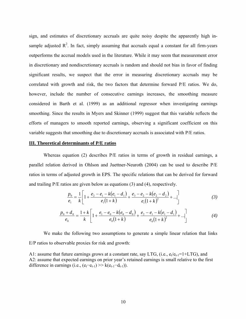
III. Theoretical determinants of P/E ratios

Whereas equation (2) describes P/E ratios in terms of growth in residual earnings, a

parallel relation derived in Ohlson and Juettner-Neuroth (2004) can be used to describe P/E

ratios in terms of adjusted growth in EPS. The specific relations that can be derived for forward

and trailing P/E ratios are given below as equations (3) and (4), respectively.

( )( )

( )( ) ⎥

⎦

⎤⎢⎣

⎡+

+−−−

++

−−−+= ...

1111

21

2223

1

1112

1

0

kedekee

kedekee

kep (3)

( )( )

( )( ) ⎥

⎦

⎤⎢⎣

⎡+

+−−−

++

−−−+

+=

+ ...11

112

0

1112

0

0001

0

00

kedekee

kedekee

kk

edp (4)

We make the following two assumptions to generate a simple linear relation that links

E/P ratios to observable proxies for risk and growth: A1: assume that future earnings grows at a constant rate, say LTG, (i.e., et/et-1=1+LTG), and A2: assume that expected earnings on prior year’s retained earnings is small relative to the first difference in earnings (i.e., (et−et-1) >> k(et-1−dt-1)).

11

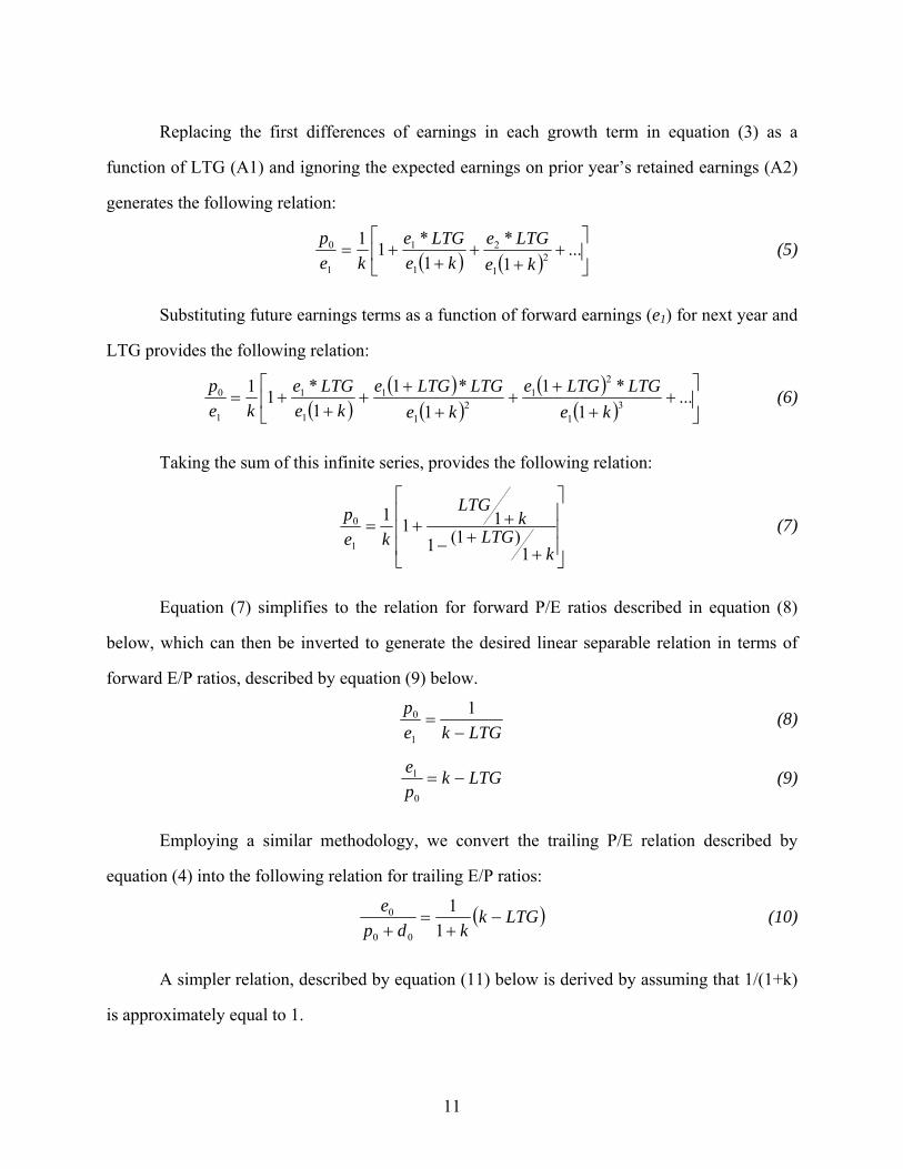
Replacing the first differences of earnings in each growth term in equation (3) as a

function of LTG (A1) and ignoring the expected earnings on prior year’s retained earnings (A2)

generates the following relation:

( ) ( ) ⎥⎦

⎤⎢⎣

⎡+

++

++= ...

1*

1*11

21

2

1

1

1

0

keLTGe

keLTGe

kep (5)

Substituting future earnings terms as a function of forward earnings (e1) for next year and

LTG provides the following relation:

( )( )

( )( )

( ) ⎥⎦

⎤⎢⎣

⎡+

++

++

++

++= ...

1*1

1*1

1*11

31

21

21

1

1

1

1

0

keLTGLTGe

keLTGLTGe

keLTGe

kep (6)

Taking the sum of this infinite series, provides the following relation:

⎥⎥⎥

⎦

⎤

⎢⎢⎢

⎣

⎡

++−

++=

kLTG

kLTG

kep

1)1(1

111

1

0 (7)

Equation (7) simplifies to the relation for forward P/E ratios described in equation (8)

below, which can then be inverted to generate the desired linear separable relation in terms of

forward E/P ratios, described by equation (9) below.

LTGke

p−

=1

1

0 (8)

LTGkpe

−=0

1 (9)

Employing a similar methodology, we convert the trailing P/E relation described by

equation (4) into the following relation for trailing E/P ratios:

( )LTGkkdp

e−

+=

+ 11

00

0 (10)

A simpler relation, described by equation (11) below is derived by assuming that 1/(1+k)

is approximately equal to 1.

12

LTGkdp

e−=

+ 00

0 (11)

Note that assumption A1 when applied to the derivation of the simplified trailing E/P

relation in equation (11) requires the additional assumption that e1/e0=1+LTG. We will show

later that this assumption is reasonable when actual earnings (e0) is taken from IBES, but less

reasonable when actual earnings is from Compustat. Also while the trailing E/P ratio is properly

calculated cum-dividend (p0+d0 in the denominator), we show later that the ex-dividend version

of the ratio typically used in practice provides very similar results.

There is no direct role for volatility of reported earnings in these relations. Therefore, any

observed relation between P/E ratios and earnings volatility should be indirect in the sense that it

should be due to other factors that link the components of earnings volatility with risk and

growth. For example, smoothing due to nondiscretionary accruals, which are likely to be

determined by industry-specific GAAP effects and production/investment/financing decisions,

may be greater in industries that are associated with high growth and low risk, resulting in higher

P/E ratios in those industries.2 Similarly, smoothing due to discretionary accruals may be greater

for firms associated with high growth and low risk.

To determine if cash flow volatility and smoothing due to accruals are related to forward

P/E ratios, we estimate regressions of E/P on cash flow volatility and reported earnings volatility.

A positive coefficient on earnings (cash flow) volatility suggests that smoothing due to accruals

(lower cash flow volatility) is associated with higher forward P/E ratios. To understand better

any links observed in the E/P regressions, we estimate regressions of forecast growth and risk on

the same regressors. A negative coefficient on earnings (cash flow) volatility in the growth

regression suggests that smoothing due to accruals (lower cash flow volatility) is associated with

higher growth forecasts. A positive coefficient on earnings (cash flow) volatility in the risk

2 By forming within-industry groups of firms with high and low smoothing due to nondiscretionary accruals,

Hunt et al. (2000) may have created a bias against finding a significant effect of such nondiscretionary smoothing on their earnings coefficients.

13

regression suggests that smoothing due to accruals (lower cash flow volatility) is associated with

lower risk.

IV. Sample Formation and Variable Definitions

Our sample is drawn from the intersection of monthly CRSP return files, quarterly

Compustat data files (industrial, research and full coverage), and summary and detail IBES files.

We conduct our analysis at the quarterly level, rather than at the annual level, to increase sample

size and to estimate our volatility measures over shorter time periods to reduce potential

problems due to non-stationary firm attributes. The IBES summary file, with consensus analyst

forecasts for different horizons as of the middle (the Thursday following the second Friday) of

each month, is used to identify the set of monthly observations available before the end of each

firm quarter. These IBES observations include forecast EPS for the current and future fiscal

years and forecast EPS growth, actual EPS for the prior four quarters, and prices. We obtain cash

flows and actual EPS data for the prior four quarters from Compustat. The IBES actual EPS

measure removes some one-time items from the EPS number reported by Compustat. In effect, it

measures permanent earnings with less error than the Compustat EPS. Details of the

computations for all variables used in our study are provided in the Appendix.

The following is a description of the main variables we consider. We examine three

measures of E/P ratios. The first is the forward E/P ratio (EPS2P), which measures the ratio of

EPS forecast for the next full year, scaled by current price as of the IBES date. The second is the

traditional trailing E/P ratio (CEP), which measures the ratio of the sum of EPS reported on

Compustat for the most recent quarter and the three quarters before that to current price. The

third is a “normalized” trailing E/P ratio (IBESEP), which is similar to CEP, except it uses actual

EPS as reported by IBES, rather than Compustat. For the latter two trailing E/P ratios we also

calculate cum-dividend versions of the ratio by adding dividends paid during the year to the ex-

dividend price, and refer to the cum-dividend trailing ratios based on Compustat EPS and IBES

EPS as CEP+D and IBESEP+D.

14

We considered two measures of the time-series volatility of reported earnings based on

two different assumptions of how earnings evolve. First, we follow the conventional wisdom

frequently mentioned in the popular financial press and assume that EPS follows a trend process,

with earnings reverting toward that trend. Our measure of volatility (STDERR) is the standard

error of the regression of annualized EPS numbers on time for that quarter and the prior 11

quarters. We use annualized or rolling four-quarter EPS numbers, corresponding to EPS for this

quarter plus the prior 3 quarters, to control for seasonal effects. There is, however, considerable

research suggesting the presence of a substantial seasonal random walk component in quarterly

earnings (e.g. Watts and Leftwich, 1977). To better represent this process, our second measure of

earnings volatility is the standard deviation of seasonally-differenced quarterly earnings

(SDSRW), over the prior 12 quarters. Since the two measures are highly correlated and the results

are not sensitive to the particular measure of earnings volatility used, we report results only for

the first measure.

We measure earnings volatility using the time-series of actual EPS as reported by IBES

since we believe that volatility induced by items that are clearly visible to the market as being

transitory are less likely to be relevant. Specifically, we hope to exclude large increases in

volatility caused by one-time items (e.g., write-offs and restructuring). In essence, our measure

would classify a firm that smoothes reported earnings in most quarters but reports a large

negative accrual occasionally as having smooth earnings, whereas a measure based on

Compustat EPS would classify it as having volatile earnings. As IBES adjusts all data for stock

splits and dividends, firm-quarters that split subsequently have smaller magnitudes for actual

EPS. If these firms that split more often also have higher P/E, these lower levels of split-adjusted

EPS will result in lower measured volatility, and create a spurious negative relation between

volatility and P/E ratios. We reverse the split adjustment made by IBES, by multiplying all

variables by the split adjustment factor. However, when computing time-series volatility, we

ensure that the prior quarters used are on the same split-adjusted basis as the current quarter.

15

Our measure of the time-series volatility of cash flows (STDCFO) is calculated as the

standard error of the regression of rolling four-quarter operating cash flows per share on time,

over the prior 12 quarters. As with STDERR, the earnings volatility measure, adjustments are

made to ensure that stock splits within the 12-quarter period do not affect measured volatility.

Since the economic value of one share is somewhat arbitrary, given that it can be changed

by stock splits, and varies across firms and over time, the volatility of per share earnings and

cash flows should properly be deflated for scale differences in per share amounts. We do not

scale those per share amounts by the level of EPS or by share price since such scaling creates a

spurious negative and positive relation, respectively, with the E/P ratio (because that scaling

variable is in the numerator and denominator, respectively, of the . We elected instead to follow

the procedure recommended by Barth and Kallapur (1996) and include total assets per share

(SCALE) as an additional regressor. This way, any differences across firm-quarters in the

magnitudes of per share amounts are controlled for by SCALE, and should not bias the estimated

regression coefficients on earnings and cash flow volatility.

To provide an estimate of the extent to which smoothing due to discretionary accruals

explains variation in E/P ratios, we include UPEARN, the measure of managerial efforts to

smooth reported earnings used in Barth et al. (1999). It is the number of consecutive earnings

increases (positive seasonally-differenced quarterly IBES EPS) during the previous 12 quarters.

A positive relation between UPEARN and forward P/E ratios suggests that discretionary accruals

are associated with forward P/E ratios.

We consider two traditional measures of risk: a) MEDBETA (computed by regressing the

previous 36 monthly returns on the equally weighted market return of all firms listed on NYSE,

AMEX, and NASDAQ, and then assigning the median beta for each beta decile to all firms in

that decile) and b) STDRET (standard deviation of monthly returns over the prior 48 months).3

We use MEDBETA, rather than the firm-specific estimates of beta (BETA), because

3 We require non-missing data for all 36 monthly returns when calculating MEDBETA.

16

examination of the distribution of BETA indicates considerable variation in beta estimates in the

extreme deciles; using MEDBETA reduces some of that measurement error. We also include two

risk measures that have been introduced recently into the literature as potential risk factors (e.g.,

Fama and French, 1992): a) SIZE (log of market value of equity as of the current quarter end)

and b) LOGBP or log of the book-to-market ratio (book value divided by the market value at the

current quarter end). Since we use SIZE as a control variable in some tests, it is not always

viewed as a risk proxy.

Our primary growth measure is the mean long-term EPS growth forecast by analysts

(LTG). That forecast is commonly assumed to refer to the growth in EPS expected over the

current year (EPS1) and the next four future years (EPS2 to EPS5). For purposes of comparison,

we also consider the traditional growth measure used in prior P/E studies, based on EPS growth

actually observed in future years (REALGR). To calculate this growth measure, we regress

rolling 4-quarter actual EPS, obtained from IBES, on time over the following 12 quarters, and

use the slope of this regression as a proxy for REALGR. Given the sharp reduction in sample

size that occurs for each additional future year included to compute REALGR, we chose three

rather than five future years for the period over which observed future growth is measured.

To be included in the sample, firm-quarters must have non-missing values for all primary

variables. There is a considerable reduction in sample size due to missing values of the cash flow

volatility variable, since operating cash flows are not reported for some industries and was first

required after 1987. To control for outliers, we impose the following filters: a) all three E/P

measures must lie between 0 and 1,4 b) the growth measure must lie between 0 and 50 percent,

c) the top and bottom 1 percent of the distributions for cash flow volatility and earnings volatility

are eliminated. Our sample includes 41,458 firm-quarter observations from 1992:I to 2002:IV.

The number of observations in the different quarters ranges from 247 for 1992:I to 1,113 for

2000:II. Despite the large sample collected, the systematic deletion of certain years and

4 This requirement, which affects Compustat E/P to the greatest extent, is imposed to minimize the impact of

observations with large negative or positive transitory earnings components.

17

industries as well as the other filters we impose potentially affect the extent to which our results

can be generalized.

V. Results

Our first analysis compares the 10-year government treasury bond yield (proxy for the

long-term risk-free rate) with the ratio of forecast earnings to price aggregated across all firms

with available data on IBES. This comparison is informally referred to as the “Fed Valuation

Model” (Greenspan, 1997) and investigates the positive relation between forward E/P (EPS2P)

and k predicted in equation (9). The period spanned is from January 1976 to March, 2005. (Note

that this sample differs from the main sample used for our other tests.).To provide evidence on

the fit of the trailing E/P ratio relation, predicted in equation (11), we provide the corresponding

time-series for IBESEP and CEP; whereas the series for IBESEP is monthly, the CEP series is

based on annual observations. When reading the figure, note that the marker for the CEP series

for 1978, for example, which is reported just to the left of the 1979 marker on the horizontal axis,

is based on earnings and dividends for firm-years ending in December, 1978, as well as all fiscal

year-ends between June, 1978 and May, 1979, and the prices are as of the end of 1978.5

The results reported in Figure 1 indicate that the 10-year risk-free rate is very highly

positively correlated with market-level forward E/P ratios, which is consistent with the relation

between E/P ratios and k predicted by equation (9). While the observed correlation is weaker for

the two trailing E/P ratios, the comovement is evident for both CEP and IBESEP.

Turning to our firm-level analyses, we report in Table 1 the pairwise correlations among

the different variables for our main sample. Pearson correlations are reported above the main

diagonal, and Spearman (rank) correlations are reported below the main diagonal. Given the

5 Even though Compustat covers more firms than IBES, the two sets of E/P ratios are comparable because of the

larger firms that are included in both samples (confirmed by comparing the dividend yield series for the Compustat and IBES samples).

18

large sample size, almost all reported correlations are significant at the 5 percent level (the few

insignificant correlations are highlighted in bold). Since the pooled regressions we estimate

combine data from different quarters with different interest rate regimes (relevant for the level of

k, which in turn affects the level of E/P), we also include the level of the risk-free rate

(RFRATE), represented by the yield on 10-year Treasury bonds. The Pearson and Spearman

correlations between different pairs of variables are generally consistent (i.e., when significant,

they are of the same sign).

The pairwise correlations among forward E/P, trailing E/P according to IBES, and

trailing E/P according to Compustat suggest that all three variables are strongly positively

related. The relations in equations (9) and (11) predict that all three E/P measures should be

positively related to the risk-free rate (RFRATE), positively related to risk (indicated by negative

correlation with SIZE and positive correlation with MEDBETA, LOGBP, and STDRET) and

negatively related to growth (LTG). The results suggest that the risk-free rate is only weakly

positively related to forward E/P and is negatively related to the two trailing E/P measures. We

conjecture that the apparent inconsistency between these results and Figure 1 is due partially to

our sample being limited to the years after 1992. (The co-movement between RFRATE and E/P

ratios in Figure 1 appears weaker for years after 1992.) Whereas all three E/P ratios exhibit the

predicted negative relation with forecast growth, and also the predicted positive relation with risk

for two of the risk measures (SIZE and LOGBP), the correlations with the other two risk

measures suggest the opposite relation. The correlations among the four risk measures suggest

inconsistencies: whereas the relation between SIZE and the other three measures is consistent

(significant negative correlation), the correlation between LOGBP and the remaining two

measures (RISK and STDRET) is not consistent.

All three E/P measures are also strongly positively correlated with the earnings volatility

measure (STDERR) and the cash flow volatility measure (STDCFO), consistent with higher P/E

ratios for smoother earnings. As expected, both volatility measures are positively related to

SCALE; i.e., larger per share total assets are associated with larger per share earnings and cash

19

flows and also with larger volatilities of per share earnings and cash flows. The measure of

managerial smoothing via discretionary accruals (UPEARN) is generally negatively related to

E/P (except for Compustat trailing E/P), suggesting that managerial smoothing is associated with

higher P/E ratios. The growth measure is positively associated with smoother earnings

(negatively related to cash flow and earnings volatility and positively related to managerial

smoothing). The risk measures, however, are not uniformly negatively related to smoother

earnings, proxied by lower cash flow and earnings volatility and higher UPEARN. Overall, the

results in Table 1 are consistent with higher P/E ratios being associated with higher growth and

with smoother earnings; the relations with interest rates and risk vary across the E/P ratios and

measures of risk, however. Since these bivariate correlations could potentially be proxying for

omitted correlated variables, a more representative picture of incremental effects of the relevant

variables is provided when we consider multiple regressions later.

Given the importance of our assumption A1 (that growth in EPS in each future year can

be proxied by LTG) to the forward and trailing E/P relations derived in equations (9) and (11),

we examine next the relation between LTG and the growth projected by analysts for each year

over the next five years. We are particularly concerned about the relation between LTG and the

growth implied from the EPS reported for the past full year (year 0) to the EPS forecast for the

current year (year +1). To the extent the two growth rates deviate from each other, assumption

A1 is less appropriate for the trailing E/P ratio relation described by equation (11), relative to

that for the forward E/P ratio relation described by equation (9). We collect a sample of firms

with summary EPS forecasts available for all years +1 to +5 as well as LTG forecasts. As might

be expected, this sample of firms consists of larger firms than our main sample. We regress log

of (1+LTG) on the log of the ratio of EPS for each future year to EPS for the prior year (e1e0,

e2e1, and so on through e5e4). The results are provided in Table 2, with Panels A and B

corresponding to EPS for year 0 being based on IBES EPS and Compustat EPS, respectively. If

the growth implied by forecasts in each year from +1 to +5 is exactly equal to LTG, the

coefficient on EPS growth in the first five simple regressions would equal 1. Since implied

20

growth over future years is unlikely to be a constant, the composite LTG is likely to deviate from

the implied future growth in each future year, thereby biasing those coefficients toward zero.6 To

the extent that LTG does not describe the growth from year 0 to year 1, the coefficient on e1e0

will be lower still. The main conclusion from Table 2 is that while LTG is generally similarly

related to all forecast growth rates from +1 to +5, since the coefficients are comparable across

those yearly growth rates, the coefficient is considerably smaller for e1e0 in Panel B. Therefore,

assumption A1 appears to be generally satisfied for the trailing E/P relation described by

equation (11) when it is based on IBES actual EPS; LTG does not, however, describe as well as

the EPS growth from year 0 to year 1, when year 0 EPS is Compustat EPS.

Ability of growth and risk to explain variation in P/E ratios

Table 3 contains the results of pooled regressions of trailing and forward E/P on the risk-

free rate (RFRATE) and the various growth and risk proxies described above. Regressions 1

through 4 are for trailing E/P ratios based on Compustat EPS, regressions 5 through 8 are for

trailing E/P ratios based on IBES actual EPS, and regressions 9 through 11 are for forward E/P

ratios. The risk-free rate is included as a regressor in each case, and for each regression we report

the estimated coefficient and associated p-value. Since those p-values do not consider

autocorrelation in residuals, they are unreliable and are provided only for completeness. The first

regression in each of the three blocks considers observed EPS growth (REALGR) and median

decile betas (MEDBETA). The second regression in each block replaces REALGR with forecast

EPS growth (LTG). The third regression adds the second traditional risk measure, representing

the standard deviation of returns (STDRET). The fourth regression in the first two blocks

considers the impact of using cum-dividend rather than ex-dividend price when calculating

trailing E/p ratios.

These results provide the following inferences. First, the coefficient on RFRATE is

significant and positive only for the three forward E/P regressions. As suggested by the bivariate

6 We provide the multiple regression (#6) in the two panels of Table 2 to complete this descriptive exercise.

21

correlations in Table 2, trailing E/P ratios are not positively related to risk-free rates at the firm

level over this sample period. Second, whereas the coefficient on REALGR is negative and

significant, as predicted by equations (9) and (11), the magnitude of that coefficient is much

lower and the adjusted R2 for those regressions is also much lower, relative to the coefficient

values and adjusted R2 observed for the corresponding regressions based on forecast growth.

Third, switching from REALGR to LTG switches the sign on MEDBETA from unexpectedly

negative to the significant positive coefficients predicted by equations (9) and (11). Fourth, while

the magnitude of the coefficient on MEDBETA is reduced when STDERR is introduced, it

remains significantly positive. The coefficient on STDERR is always significant and positive as

predicted. Finally, there appears to be no improvement in the fit of the full regressions for the

two trailing E/P ratios when ex-dividend prices are replaced by the cum-dividend prices noted in

equation (11).

The most important finding from Table 3 is the improvement in fit when the observed

growth measure used in earlier studies on the determinants of P/E ratios is replaced by the

forecast growth measure more recently. Not only does observed growth measure anticipated

growth with considerable error, indicated by lower estimated coefficients on growth and lower

adjusted R2, that measurement error appears to be systematically related to risk measures which

causes inconsistent relations between P/E ratios and risk.

To provide p-values for the coefficient estimates that are corrected for potential

autocorrelation among regressions residuals, we estimate cross-sectional regressions by fiscal

quarter and report the mean values of those coefficients as well as the p-values associated with 2-

tailed tests based on Newey-West (1987) corrections for autocorrelation in the deviation of the

estimated coefficients around that mean. Those results are provided in Table 4. We collect each

cross-section by fiscal quarter to allow for the possibility that different fiscal quarters are

fundamentally different from each other. Even though there is some variation in interest rates

across observations in the same cross-section (because of cross-sectional variation in fiscal year-

22

ends), variation in RFRATE is largely suppressed and the associated coefficients are likely to be

insignificant. As in Table 3, we repeat the analyses for trailing E/P ratios based on Compustat

EPS (regressions 1 and 2), trailing E/P ratios based on IBES EPS (regressions 3 and 4), and

forward E/P ratios (regressions 5 and 6). The first regression in each block is a reduced

specification that considers only the growth proxy (LTG) and the first risk proxy considered in

Table 3 (MEDBETA), and the second regression also considers STDERR and the two more

recent risk proxies (LOGBP and SIZE).

The inferences from Table 4 can be summarized as follows. First, as expected, the

sharply reduced variation in RFRATE for quarter-by-quarter regressions makes the associated

coefficient insignificant, except for regression 6 where the coefficient is significantly positive.

Second, the coefficient on LTG is always significant and negative as predicted. Third, the

coefficient on MEDBETA, which was significant and positive in the reduced specifications in

Table 3 is associated with higher p-values, because of the Newey-West corrections. While those

higher p-values cause the coefficient to be insignificant in the case of CEP, it remains significant

for the trailing E/P ratio based on IBES EPS and for forward E/P ratios. Fourth, the coefficient

on MEDBETA becomes insignificant when the other risk proxies are introduced in the full

specification; the three additional risk proxies are, however, statistically significant with signs

consistent with the predicted relations in all three blocks.

We conclude the first part of our analysis by summarizing our main findings regarding

the relation between P/E ratios and its theoretical determinants (interest rates, risk, and growth).

At the firm level, both trailing and forward E/P ratios are strongly related to forecast earnings

growth and measures of risk. While market model beta is significantly positively related to E/P

ratios when it is the only risk measure considered, it becomes insignificant in the presence of

other proxies for risk. Using observed EPS growth as a proxy for anticipated earnings growth

creates substantial misspecification: growth is measured with considerable error and risk appears

with the wrong sign. The predicted positive association between E/P ratios and interest rates is

23

observed only for forward E/P ratios, suggesting that the forward E/P ratio regressions are better

specified than those based on trailing E/P ratios.

Earnings volatility and variation in P/E ratios

Before estimating the impact of cash flow volatility and smoothing due to accruals on P/E

ratios, we first provide descriptive statistics for decile portfolios formed each quarter based on

the volatility of reported earnings. Table 5 contains the mean values of different variables that

measure growth, risk, cash flow volatility, and E/P ratios for deciles based on STDERR. By

allowing a closer look at how the different relations vary across partitions of earnings volatility,

this analysis serves as a complement to the pair-wise correlations described in Table 1.

There is a monotonic negative relation between earnings volatility and LTG, suggesting

that firms with smoother reported earnings are associated with higher forecast EPS growth. Since

reported earnings volatility reflects both the volatility of cash flows as well as the smoothing due

to accruals, this negative relation between earnings volatility and growth could be due to high

growth firms being associated with smoother underlying cash flows and/or greater smoothing

due to accruals. The relation between earnings volatility and SIZE suggests a shallow U-shape,

where firms with extreme volatility are slightly larger than firms with intermediate volatility. To

the extent the next three measures (LOGBP, STDRET, and MEDBETA) are risk proxies, they all

indicate a positive relation between earnings volatility and risk, suggesting again that less risky

firms could be associated with smoother cash flows and/or greater smoothing due to accruals.

The results reported under the columns UPEARN and STDCFO confirm that cash flow

volatility and smoothing due to discretionary accruals, two components of reported earnings

volatility, are positively related to earnings volatility. There is a large spread between the top and

bottom earnings volatility decile for both variables. The relations reported in the next three

columns confirm the correlations reported in Table 1: firms with less volatile reported earnings

are valued more highly per dollar of earnings (have lower E/P ratios). The spread between the

top and bottom deciles is highest for forward E/P and lower for the trailing E/P measures. Also,

24

the relation is less linear for the two trailing E/P measures (a steeper gradient is observed for the

two top and bottom deciles and is quite flat for the remaining deciles). Finally, contrary to our

initial concern that scale effects may cause firms with more volatile earnings to be larger on a per

share basis, we find that SCALE (measured by total assets per share) is actually negatively

related to earnings volatility.

Table 6 contains the results of estimating our first set of regressions that link earnings

volatility with E/P ratios. We investigate first whether cash flow volatility and smoothing due to

accruals are related to E/P ratios, and then consider how those relations are altered in the

presence of proxies for risk and growth. Our methodology is to include both cash flow volatility

and earnings volatility, and the coefficient on earnings volatility captures the effect of smoothing

due to accruals. The dependent variable is Compustat trailing E/P ratios, IBES trailing E/P ratios,

and forward E/P ratios in Panels A, B, and C, respectively. We report three values in each cell:

the coefficient from a pooled regression, the mean value of the coefficients estimated in the

quarter-by-quarter regressions, and the p-value from a two-tailed test based on the distribution of

coefficients from quarter-by-quarter regressions that has been adjusted for autocorrelation using

the Newey-West procedure.

In each panel of Table 6, we begin with cash flow volatility and a control for scale

(STDCFO and SCALE in regression 1), and then in incremental steps add RFRATE and SIZE (in

regressions 2 and 3). We include SIZE, not as a risk measure, but as a general control for factors

that may cause measurement error in our volatility measures. (Our main results are not sensitive

to the inclusion or exclusion of SIZE.) Regression 4, which includes the volatility of reported

earnings (STDERR), represents our main result in each panel. The next model (regression 5)

considers the impact of including UPEARN, the measure of smoothing due to discretionary

accruals. To the extent that smoothing due to discretionary accruals plays a substantial role,

UPEARN will be significantly negative and the importance of STDERR should be reduced. The

final model (regression 6) includes the three risk measures excluded so far (STDRET, LOGBP,

and MEDBETA) and our growth measure (LTG). Since cash flow and earnings volatility as well

25

as earnings smoothing due to discretionary accruals do not appear as factors that determine P/E

ratios in equations (2) and (4), we expect the coefficients on cash flow and earnings volatility as

well as the coefficient on UPEARN to become insignificant in regression 6.

We begin with an overview of the results and trends that are observed in all Panels. First,

E/P is positively related to cash flow volatility (STDCFO) in regression 1, and we continue to

observe a significant positive coefficient on STDCFO even after we include other variables in the

subsequent regressions. Second, the coefficient on RFRATE is generally insignificant in the

quarter-by-quarter regressions. Third, the coefficient on SIZE is always negative and significant.

Fourth, the coefficient on STDERR is generally positive and significant in Panels A and C, but is

insignificant in Panel B for trailing E/P ratios based on actual IBES EPS. This suggests that

earnings smoothing due to accruals is generally associated with higher P/E ratios. Fifth, the

coefficient on UPEARN is generally significantly positive, which suggests that managerial

smoothing based on discretionary accruals being used to report a string of earnings increases is

negatively related to P/E ratios. We are unable to identify which of the many differences between

our study and Barth et al. (1999) causes this difference in results. Finally, the coefficients on the

additional risk and growth proxies introduced in regression 6 in each panel are of the predicted

sign and statistically significant (except for MEDBETA which is insignificant).

The main conclusion from these results is that lower cash flow volatility and reduced

earnings volatility due to accruals are both generally related to higher P/E ratios. More important,

while these relations weaken slightly in the presence of controls for risk and growth, the

coefficient on cash flow volatility is significant in all three panels, and the coefficient on

earnings volatility is significant at the 5 percent level in Panel A and at the 10% level in Panel C.

Since cash flow an earnings volatility are missing in the theoretical relation for P/E ratios, these

empirical results suggest either that the theoretical model is incomplete, or that the risk and

growth proxies we use are incomplete. Although we are unable to discriminate between these

two explanations, we lean toward concluding that our proxies only partially capture the impact of

risk and growth and as a result cash flow and earnings volatility appear as significant

26

determinants of P/E ratios because they are correlated with risk and growth. The next analysis

examines this possibility by considering the links between risk/growth and cash flow and

earnings volatility.

Table 7 contains the results of regressing different growth and risk measures on cash flow

volatility, earnings volatility, and UPEARN, our measure of smoothing due to discretionary

accruals. The dependent variables in Panels A, B, C, and D are LTG, BETA, STDRET, and

LOGBP, respectively. For each regressor, we provide the coefficient from a pooled regression,

the mean coefficient from quarter-by-quarter regressions, and the p-value from a two-tailed test

based on the distribution of coefficients from quarter-by-quarter regressions that has been

adjusted for autocorrelation using the Newey-West procedure. The first regression in each panel

examines whether cash flow volatility and smoothing due to accruals are related to growth/risk,

the second regression checks to see whether those results are sensitive to the addition of SIZE as

a control variable, and the third regression reports on the impact of including UPEARN or

smoothing due to discretionary accruals.

The results in Panel A of Table 7 indicate that growth forecasts are strongly negatively

related to cash flow volatility and positively related to earnings smoothing due to accruals

(indicated by significant, negative coefficients on cash flow volatility and reported earnings

volatility, respectively, in the first regression). These results provide a partial explanation for the

relations between forward P/E ratios and components of earnings volatility observed in Table 6.

Incorporating SIZE in the second regression does not alter the inferences regarding growth and

earnings volatility components; the significant negative coefficient on SIZE suggests that firms

with smaller market capitalization are associated with higher EPS growth forecasts. The positive

and significant coefficient on UPEARN in the third regression confirms that this measure of

earnings smoothing is incrementally associated with higher growth. The coefficient on STDERR

remains negative and significant, but declines substantially, which suggests that a substantial

fraction of the relation between growth and smoothing due to accruals is due to the discretionary

accruals covered by UPEARN. That is, firms that smooth earnings by reporting sustained

27

earnings increases are associated with higher growth. While this relation would suggest that

UPEARN should also be positively related to P/E ratios, the results in Table 6 suggest the

opposite relation.

The results in Panel B of Table 7 indicate that BETA risk decreases with greater

smoothing due to accruals (positive coefficient on STDERR), but they also suggest that BETA

risk decreases with cash flow volatility (negative coefficient on STDCFO). These results provide

at best a partial explanation for the relations between higher P/E ratios and components of

earnings volatility observed in Table 6. The tenor of the results is not affected by the inclusion of

SIZE in the second regression. The coefficient on UPEARN in the third regression is

insignificant, indicating no clear incremental relation between smoothing due to discretionary

accruals and risk. Overall, our results regarding BETA are mixed: only one component of

reduced earnings volatility (smoothing due to accruals) is related to lower risk, and the remaining

results are inconsistent with the strong relation observed between reduced earnings volatility and

higher P/E ratios.

The results in Panel C of Table 7 for the volatility of returns are similar to those observed

for BETA. While lower volatility of stock returns is associated with greater smoothing due to

accruals (positive coefficient on STDERR), lower volatility of cash flows and greater smoothing

due to discretionary accruals are associated with higher risk (indicated by a negative coefficient

on STDCFO and positive coefficient on UPEARN). Again, these results provide at best only a

partial explanation for the strong relation observed between reduced earnings volatility and

higher P/E ratios.

The results in Panel D of Table 7, relating to the B/P ratio, provide results that are

consistent with the observed link between reduced earnings volatility and higher P/E ratios.

Lower cash flow volatility, greater smoothing due to accruals, and greater smoothing due to

discretionary accruals are all associated with lower risk (indicated by significant positive,

positive, and negative coefficients on STDERR, STDCFO, and UPEARN, respectively). Unlike

the mixed results observed in Panels B and C, these results are similar to those observed for

28

growth in Panel A, and suggest that both risk and growth are associated with earnings volatility,

which explains the observed relation between earnings volatility and forward P/E ratios.

Overall, the residual relation observed in Table 6 between P/E ratios and the two

components of reduced earnings volatility—lower cash flow volatility and earnings smoothing

due to accruals—can be explained as follows. Both volatility measures are related to growth and

risk, and they are thus related to P/E ratios. While introducing proxies for risk and growth to

those regressions reduces the observed relation between the volatility measures and P/E ratios, it

does not eliminate it because the proxies we use do not completely capture the effect of risk and

growth.

VI. Conclusion

This study is motivated by the apparent gap between the weak links observed in earlier

research investigating the cross-sectional determinants of P/E ratios and the stronger links

suggested by recent research estimating the cost of capital. We find that the weak and

inconsistent links documented in prior research are due primarily to the use of observed prior

earnings growth; replacing that growth proxy with forecast earnings growth resolves a

substantial amount of this gap. A second factor that explains a smaller portion of this gap is the

use of forward rather than trailing P/E ratios in recent research.

We also examine the relation between P/E ratios and reported earnings volatility, which

can be represented by underlying cash flow volatility and the reduction in that volatility because

of accruals. While the relations derived for P/E ratios contain no explicit role for earnings

volatility, prior empirical research (e.g., Barth et al., 1999 and Hunt et al., 2000) suggests that

managerial efforts to reduce the volatility of reported earnings by undertaking discretionary

accruals designed to smooth out spikes in unmanaged earnings are associated with higher

earnings coefficients in estimated price-earnings relations. Two possible explanations for this

result are as follows: a) managerial smoothing reduces the error with which reported earnings

measure value-relevant permanent earnings, and b) managerial smoothing is associated with

29

firms that have higher growth and lower risk. While the prior research has focused on the

measurement error explanation, we focus on the second explanation. To mitigate the potential

impact of measurement error, we examine regressions of E/P ratios on earnings volatility, rather

than the coefficient on reported earnings in a price-earnings regression. Given our concerns

about the ability to isolate managerial smoothing, we focus more broadly on smoothing due to

total accruals (both discretionary and nondiscretionary). We also consider whether cash flow

volatility, the remaining component of earnings volatility, is related to P/E ratios.

Our results suggest that both lower cash flow volatility and greater smoothing due to

accruals are strongly associated with higher forward P/E ratios. More important, these relations

are due largely to an underlying association between both components of earnings volatility and

risk/growth. That is, lower cash flow volatility and greater smoothing due to accruals are

associated with higher growth and lower risk, the two factors that directly determine the higher

observed P/E ratios.

We hope this paper will invigorate efforts to build a better understanding of why lower

cash flow volatility and greater smoothing due to accruals are associated with higher perceived

growth and lower perceived risk. Generally, the explanations for these results would fall into two

categories: endogenous and exogenous. The first category would contain models that predict

why in equilibrium it is optimal for managers of firms with high growth and low risk to use

discretionary accruals to smooth reported earnings. The second category would consist of

explanations that identify institutional factors and accounting rules that cause firms with high

growth and low risk to have lower cash flow volatility and greater smoothing due to

nondiscretionary accruals. It appears to be easier to build endogenous and exogenous

explanations for why firms with lower cash flow volatility and greater smoothing due to accruals

are associated with lower risk; building explanations for why they are associated with higher

growth presents more of a challenge. There has been some anecdotal and empirical evidence,

which suggests possible avenues that theory might consider. First, firms with better prospects

(such as Microsoft and GE) are alleged to build reserves by choosing conservative accounting

30

methods and estimates and then smooth earnings to report a steadily rising stream. The higher

P/E ratios for such firms are due to reported earnings being understated and/or higher growth in

reported earnings that is forecast for such firms. Second, firms with higher growth prospects may

face greater incentives to smooth earnings, to avoid the disproportionately large price drops in

stock price that result if earnings growth is not maintained (e.g., Skinner and Sloan, 2002).

31

Appendix Variable definitions

dataxx refers to the corresponding data item from the quarterly Compustat file and firm and market returns are from the monthly CRSP files. The IBES forecast data is taken from the summary and detailed files. All per share data from IBES is un-split-adjusted to obtain amounts reported on those dates. When calculating STDERR and STDCFO, the time-series is split-adjusted to ensure that all observations are on the same basis as the most recent quarter in the 12 quarter estimation period.

BETA (systematic risk) is the slope from a regression of monthly returns over the prior 36 months on the corresponding monthly returns of an equally weighted market index (NYSE, AMEX, and NASDAQ).

MEDBETA is the median value of BETA of the BETA decile, to which the observations belongs. The BETA deciles are formed quarterly.

SIZE (risk measure) is the natural log of market capitalization at the end of the quarter (data14 * data61).

LOGBP (risk measure) is the natural log of the book-to-market ratio, at the end of the quarter, equal to book value (data60) divided by market value (data14 * data61).

STDRET (risk measure) is the standard deviation of monthly returns over the prior 48 months.

STDERR (volatility of reported earnings) is the standard error of the regression of rolling 4-quarter EPS, from IBES (actual EPS for that quarter plus EPS for the prior three quarters) on time, estimated over the prior 12 quarters.

UPEARN (measure of managerial income smoothing) is the number of times the company reports consecutive earnings increases (positive seasonally-differenced quarterly EPS, based on actual IBES EPS) during the previous 12 quarters.

STDCFO (measure of cash flow volatility) is the standard error of the regression of rolling 4-quarter per share cash flow from operations (data108/data61) on time, estimated over the prior 12 quarters. The number of shares at each quarter end (data61) is adjusted for stock splits during the estimation period.

LTG (forecast growth measure) is the consensus (mean) long-term growth rate forecast for EPS, from the IBES summary file.

EPS2P is the forward E/P ratio, where EPS2 is the consensus (mean) two-year out EPS forecast and P is the price reported by IBES.

IBESEP is the trailing IBES E/P ratio, where IBESEPS is the actual EPS for that quarter and prior 3 quarters, and P is the price reported by IBES.

IBESEP+D is the trailing cum-dividend IBES E/P ratio, where the actual DPS for that quarter and prior 3 quarters is added to IBESEPS.

CEP is the Compustat trailing E/P ratio, where CE is the primary EPS before extraordinary items and discontinued operations for current quarter and prior three quarters, and P is the current quarter end share price reported by Compustat.

32

CEP+D is the Compustat trailing cum-dividend E/P ratio, where the actual DPS for that quarter and prior 3 quarters is added to CE.

REALGR is a measure of observed future growth in EPS, equal to the slope of a regression of rolling 4-quarter IBES EPS on time, estimated over the next 12 quarters.

SCALE is total assets per share as of the end of current quarter.

33

Figure 1 Time-series of aggregate earnings yields (E/P ratios) and Long-term Treasury yields

0%

2%

4%

6%

8%

10%

12%

14%

16%

18%

1976

1978

1980

1982

1984

1986

1988

1990

1992

1994

1996

1998

2000

2002

2004

2006

year (tick mark represents beginning of that year)

yiel

ds

10-year Risk freeIBES Forecast EarningsCompustat Trailing EarningsIBES Trailling Earnings

34

Table 1 Correlation between pairs of variables for 41,348 firm-quarters from 1992:I to 2002: IV (Pearson above main diagonal and Spearman below).

We require nonmissing values for LTG, STDCFO, STDERR, LOGBP, SIZE, MEDBETA, STDRET and UPEARN. In addition, we require that 0≤LTG≤1, and that EPS2P, IBESEP and CEP lie between 0 and 1. Finally, to control for outliers, we eliminate the top and bottom 1% of STDERR and STDCFO. EPS2P IBESEP CEP RFRATE SIZE BETA LOGBP STDRET LTG STDCFO STDERR UPEARN SCALE EPS2P 0.788 0.630 0.037 -0.362 -0.017 0.541 -0.018 -0.286 0.254 0.163 -0.103 0.143

IBESEP 0.816 0.779 -0.030 -0.216 -0.086 0.456 -0.068 -0.329 0.231 0.114 -0.052 0.158

CEP 0.672 0.813 -0.004 -0.224 -0.077 0.429 -0.062 -0.288 0.232 0.135 0.048 0.161

RFRATE 0.070 0.004 0.033 -0.077 0.116 -0.006 -0.235 -0.048 -0.008 -0.011 0.092 0.016

SIZE -0.377 -0.223 -0.233 -0.074 -0.239 -0.509 -0.271 -0.091 0.019 0.014 0.108 0.213

MEDBETA -0.016 -0.110 -0.095 0.127 -0.245 -0.022 0.504 0.422 -0.064 0.039 0.002 -0.164

LOGBP 0.593 0.491 0.455 -0.003 -0.498 -0.008 -0.005 -0.331 0.269 0.210 -0.280 0.188

STDRET -0.024 -0.131 -0.134 -0.248 -0.338 0.491 0.017 0.501 -0.089 0.065 -0.063 -0.212

LTG -0.322 -0.382 -0.336 -0.053 -0.125 0.405 -0.325 0.572 -0.218 -0.152 0.154 -0.236

STDCFO 0.297 0.255 0.238 -0.012 -0.001 -0.051 0.341 -0.081 -0.268 0.415 -0.089 0.429

STDERR 0.212 0.106 0.100 -0.021 -0.063 0.059 0.320 0.122 -0.201 0.488 -0.209 0.238

UPEARN -0.119 -0.074 0.073 0.100 0.101 0.006 -0.291 -0.055 0.159 -0.102 -0.284 -0.046

SCALE. 0.291 0.321 0.295 0.014 0.286 -0.310 0.360 -0.470 -0.518 0.569 0.329 -0.079 Notes: All correlation coefficients are significant at the 5% level, except those in bold. EPS2P is the forward E/P ratio, equal to the consensus (mean) two-year out EPS forecast scaled by price reported by IBES. IBESEP is the trailing IBES E/P ratio, equal to the actual IBES EPS for that quarter and prior 3 quarters, scaled by price reported by IBES. CEP is the Compustat trailing E/P ratio, equal to primary EPS before extraordinary items for current quarter and prior three quarters, divided by current quarter end share price. RFRATE is the risk-free rate, represented by the 10-year Treasury bond yield. SIZE is the natural log of the market value of equity at the end of the current fiscal quarter. MEDBETA is a measure of systematic risk, represented by the median decile BETA, where BETA is estimated from the market model over the prior 36 months. LOGBP is the natural log of the ratio of book value to market value of equity, at the end of the current fiscal quarter. STDRET is the standard deviation of previous 48 months’ returns. LTG is the consensus (mean) long term growth forecast for EPS. STDCFO is the standard error of the regression of rolling 4-quarter per share cash flow from operations on time, estimated over the prior 12 quarters. STDERR is the standard error from a regression of rolling 4-quarter IBES actual EPS on time, estimated over the prior 12 quarters. UPEARN reports the number of consecutive quarterly IBES actual earnings increases during the previous 12 quarters SCALE is is total assets per share as of the end of current quarter.

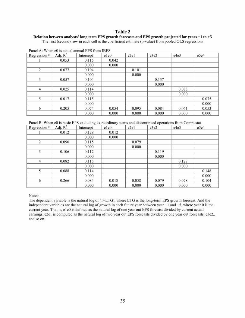
35

Table 2 Relation between analysts’ long term EPS growth forecasts and EPS growth projected for years +1 to +5

The first (second) row in each cell is the coefficient estimate (p-value) from pooled OLS regressions

Panel A: When e0 is actual annual EPS from IBES Regression # Adj. R2 Intercept e1e0 e2e1 e3e2 e4e3 e5e4

1 0.053 0.115 0.042 0.000 0.000

2 0.077 0.104 0.101 0.000 0.000

3 0.057 0.104 0.137 0.000 0.000

4 0.025 0.114 0.083 0.000 0.000

5 0.017 0.115 0.075 0.000 0.000

6 0.205 0.074 0.054 0.095 0.084 0.061 0.053 0.000 0.000 0.000 0.000 0.000 0.000 Panel B: When e0 is basic EPS excluding extraordinary items and discontinued operations from Compustat Regression # Adj. R2 Intercept e1e0 e2e1 e3e2 e4e3 e5e4

1 0.012 0.128 0.012 0.000 0.000

2 0.090 0.115 0.079 0.000 0.000

3 0.106 0.112 0.119 0.000 0.000

4 0.082 0.115 0.127 0.000 0.000

5 0.088 0.114 0.148 0.000 0.000

6 0.266 0.084 0.018 0.058 0.079 0.078 0.104 0.000 0.000 0.000 0.000 0.000 0.000 Notes: The dependent variable is the natural log of (1+LTG), where LTG is the long-term EPS growth forecast. And the independent variables are the natural log of growth in each future year between year +1 and +5, where year 0 is the current year. That is, e1e0 is defined as the natural log of one year out EPS forecast divided by current actual earnings, e2e1 is computed as the natural log of two year out EPS forecasts divided by one year out forecasts. e3e2,, and so on.

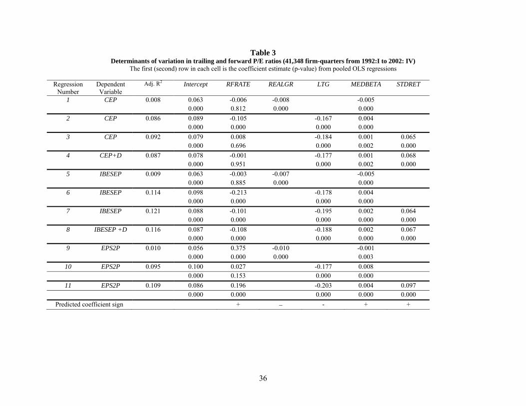
36

Table 3 Determinants of variation in trailing and forward P/E ratios (41,348 firm-quarters from 1992:I to 2002: IV)

The first (second) row in each cell is the coefficient estimate (p-value) from pooled OLS regressions

Regression Number

Dependent Variable

Adj. R2 Intercept RFRATE REALGR LTG MEDBETA STDRET

1 CEP 0.008 0.063 -0.006 -0.008 -0.005 0.000 0.812 0.000 0.000

2 CEP 0.086 0.089 -0.105 -0.167 0.004 0.000 0.000 0.000 0.000

3 CEP 0.092 0.079 0.008 -0.184 0.001 0.065 0.000 0.696 0.000 0.002 0.000

4 CEP+D 0.087 0.078 -0.001 -0.177 0.001 0.068 0.000 0.951 0.000 0.002 0.000

5 IBESEP 0.009 0.063 -0.003 -0.007 -0.005 0.000 0.885 0.000 0.000

6 IBESEP 0.114 0.098 -0.213 -0.178 0.004 0.000 0.000 0.000 0.000

7 IBESEP 0.121 0.088 -0.101 -0.195 0.002 0.064 0.000 0.000 0.000 0.000 0.000

8 IBESEP +D 0.116 0.087 -0.108 -0.188 0.002 0.067 0.000 0.000 0.000 0.000 0.000

9 EPS2P 0.010 0.056 0.375 -0.010 -0.001 0.000 0.000 0.000 0.003

10 EPS2P 0.095 0.100 0.027 -0.177 0.008 0.000 0.153 0.000 0.000

11 EPS2P 0.109 0.086 0.196 -0.203 0.004 0.097 0.000 0.000 0.000 0.000 0.000

Predicted coefficient sign + − - + +

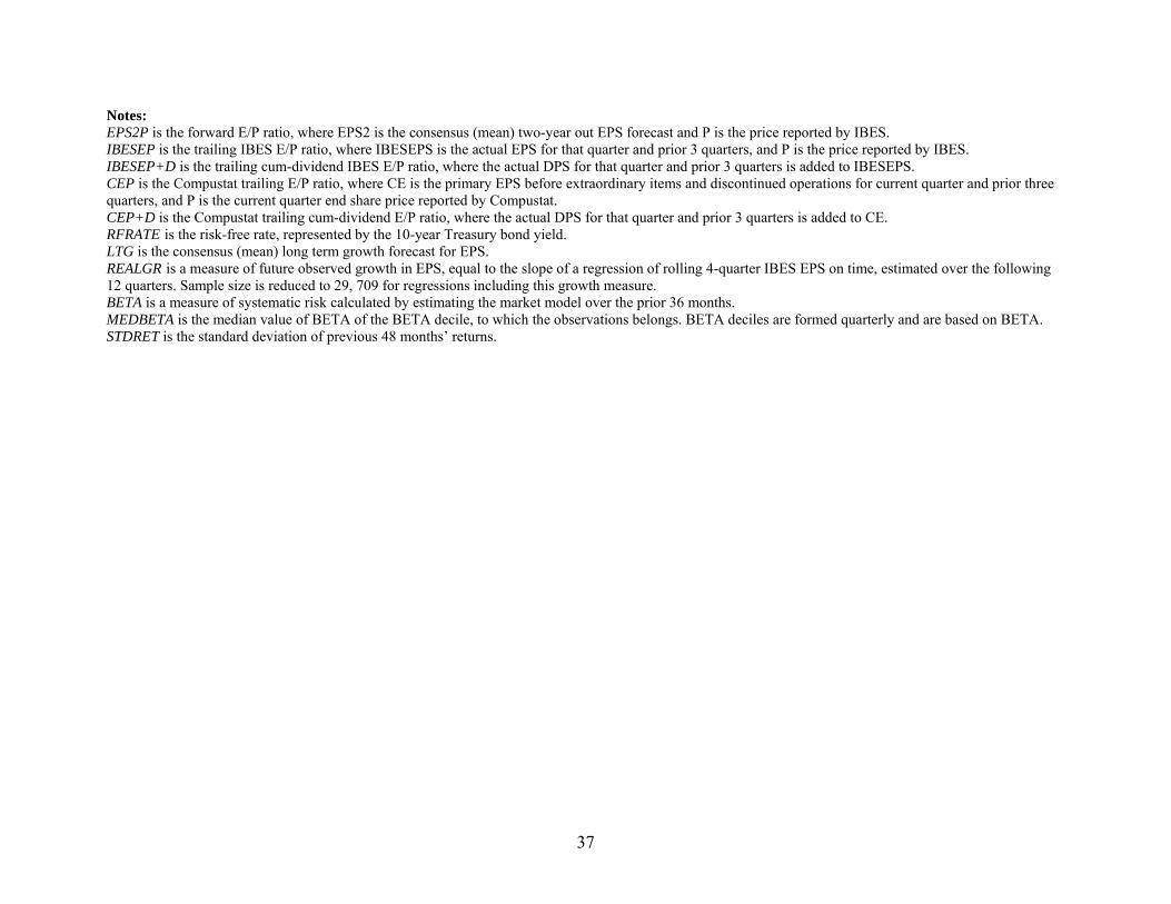
37

Notes: EPS2P is the forward E/P ratio, where EPS2 is the consensus (mean) two-year out EPS forecast and P is the price reported by IBES. IBESEP is the trailing IBES E/P ratio, where IBESEPS is the actual EPS for that quarter and prior 3 quarters, and P is the price reported by IBES. IBESEP+D is the trailing cum-dividend IBES E/P ratio, where the actual DPS for that quarter and prior 3 quarters is added to IBESEPS. CEP is the Compustat trailing E/P ratio, where CE is the primary EPS before extraordinary items and discontinued operations for current quarter and prior three quarters, and P is the current quarter end share price reported by Compustat. CEP+D is the Compustat trailing cum-dividend E/P ratio, where the actual DPS for that quarter and prior 3 quarters is added to CE. RFRATE is the risk-free rate, represented by the 10-year Treasury bond yield. LTG is the consensus (mean) long term growth forecast for EPS. REALGR is a measure of future observed growth in EPS, equal to the slope of a regression of rolling 4-quarter IBES EPS on time, estimated over the following 12 quarters. Sample size is reduced to 29, 709 for regressions including this growth measure. BETA is a measure of systematic risk calculated by estimating the market model over the prior 36 months. MEDBETA is the median value of BETA of the BETA decile, to which the observations belongs. BETA deciles are formed quarterly and are based on BETA. STDRET is the standard deviation of previous 48 months’ returns.

38

Table 4 Determinants of cross-sectional variation in trailing and forward E/P ratios (41,348 firm-quarters from 1992:I to 2002: IV)

The first (second) row in each cell is the mean coefficient estimate (p-value from two-tailed Newey-West test) from regressions estimated each fiscal quarter.

Regression Number

Dependent Variable

Mean adj. R2 Intercept RFRATE LTG MEDBETA SIZE LOGBP STDRET

1 CEP 0.111 0.088 -0.180 -0.169 0.004 <.0001 0.330 <.0001 0.000

2 CEP 0.217 0.099 -0.068 -0.115 0.000 -0.002 0.014 0.022 <.0001 0.616 <.0001 0.754 0.002 <.0001 0.001

3 IBESEP 0.139 0.081 0.006 -0.180 0.005 <.0001 0.967 <.0001 <.0001

4 IBESEP 0.251 0.088 0.111 -0.130 0.000 -0.001 0.014 0.029 <.0001 0.325 <.0001 0.704 0.024 <.0001 0.001

5 EPS2P 0.121 0.089 0.141 -0.175 0.009 <.0001 0.316 <.0001 <.0001

6 EPS2P 0.345 0.111 0.252 -0.115 0.001 -0.003 0.018 0.061 <.0001 0.024 <.0001 0.286 <.0001 <.0001 0.001

Predicted coefficient sign + − + − + + Notes: EPS2P is the forward E/P ratio, equal to the consensus (mean) two-year out EPS forecast scaled by price reported by IBES. IBESEP is the trailing IBES E/P ratio, equal to the actual IBES EPS for that quarter and prior 3 quarters, scaled by price reported by IBES. CEP is the Compustat trailing E/P ratio, equal to primary EPS before extraordinary items and discontinued operations for current quarter and prior three quarters, divided by current quarter end share price. RFRATE is the risk-free rate, represented by the 10-year Treasury bond yield. LTG is the consensus (mean) long term growth forecast for EPS. MEDBETA is the median value of BETA of the BETA decile, to which the observations belongs. The BETA deciles are formed quarterly and are based on BETA. SIZE is the natural log of the market value of equity at the end of the current fiscal quarter. LOGBP is the natural log of the ratio of book value to market value of equity, at the end of the current fiscal quarter. STDRET is the standard deviation of previous 48 months’ returns.

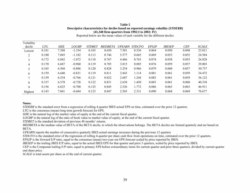
39

Table 5 Descriptive characteristics for deciles based on reported earnings volatility (STDERR)

(41,348 firm-quarters from 1992:I to 2002: IV) Reported below are the mean values of each variable for the different deciles

Volatility

decile LTG SIZE LOGBP STDRET MEDBETA UPEARN STDCFO EPS2P IBESEP

CEP

SCALE Lowest 0.181 7.388 -1.334 0.103 0.650 7.501 0.536 0.064 0.050 0.048 23.011

2 0.180 7.045 -1.182 0.113 0.746 5.577 0.665 0.069 0.053 0.052 24.584 3 0.172 6.842 -1.072 0.118 0.767 4.466 0.763 0.074 0.058 0.055 26.828 4 0.170 6.687 -0.960 0.119 0.785 3.815 0.885 0.076 0.059 0.057 29.003 5 0.165 6.568 -0.886 0.120 0.828 3.254 0.966 0.079 0.060 0.057 30.737 6 0.159 6.640 -0.831 0.119 0.811 2.843 1.114 0.081 0.061 0.059 34.472 7 0.159 6.534 -0.766 0.121 0.822 2.687 1.244 0.083 0.061 0.059 36.122 8 0.157 6.578 -0.728 0.122 0.831 2.638 1.450 0.083 0.061 0.060 40.338 9 0.156 6.625 -0.700 0.125 0.845 2.526 1.772 0.086 0.063 0.063 46.911

Highest 0.143 7.041 -0.684 0.123 0.847 2.503 2.331 0.090 0.068 0.069 70.677 Notes: STDERR is the standard error from a regression of rolling 4-quarter IBES actual EPS on time, estimated over the prior 12 quarters. LTG is the consensus (mean) long term growth forecast for EPS. SIZE is the natural log of the market value of equity at the end of the current fiscal quarter. LOGBP is the natural log of the ratio of book value to market value of equity, at the end of the current fiscal quarter. STDRET is the standard deviation of previous 48 months’ returns. MEDBETA is the median value of BETA of the BETA decile, to which the observations belongs. The BETA deciles are formed quarterly and are based on BETA. UPEARN reports the number of consecutive quarterly IBES actual earnings increases during the previous 12 quarters STDCFO is the standard error of the regression of rolling 4-quarter per share cash flow from operations on time, estimated over the prior 12 quarters. EPS2P is the forward E/P ratio, equal to the consensus (mean) two-year out EPS forecast scaled by price reported by IBES. IBESEP is the trailing IBES E/P ratio, equal to the actual IBES EPS for that quarter and prior 3 quarters, scaled by price reported by IBES. CEP is the Compustat trailing E/P ratio, equal to primary EPS before extraordinary items for current quarter and prior three quarters, divided by current quarter end share price. SCALE is total assets per share as of the end of current quarter.

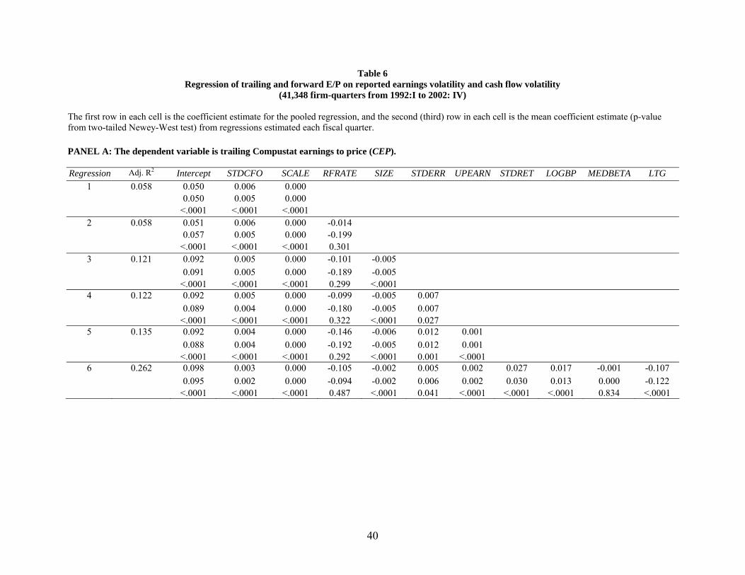
40

Table 6 Regression of trailing and forward E/P on reported earnings volatility and cash flow volatility

(41,348 firm-quarters from 1992:I to 2002: IV)

The first row in each cell is the coefficient estimate for the pooled regression, and the second (third) row in each cell is the mean coefficient estimate (p-value from two-tailed Newey-West test) from regressions estimated each fiscal quarter. PANEL A: The dependent variable is trailing Compustat earnings to price (CEP). Regression Adj. R2 Intercept STDCFO SCALE RFRATE SIZE STDERR UPEARN STDRET LOGBP MEDBETA LTG

1 0.058 0.050 0.006 0.000 0.050 0.005 0.000 <.0001 <.0001 <.0001

2 0.058 0.051 0.006 0.000 -0.014 0.057 0.005 0.000 -0.199 <.0001 <.0001 <.0001 0.301

3 0.121 0.092 0.005 0.000 -0.101 -0.005 0.091 0.005 0.000 -0.189 -0.005 <.0001 <.0001 <.0001 0.299 <.0001

4 0.122 0.092 0.005 0.000 -0.099 -0.005 0.007 0.089 0.004 0.000 -0.180 -0.005 0.007 <.0001 <.0001 <.0001 0.322 <.0001 0.027

5 0.135 0.092 0.004 0.000 -0.146 -0.006 0.012 0.001 0.088 0.004 0.000 -0.192 -0.005 0.012 0.001 <.0001 <.0001 <.0001 0.292 <.0001 0.001 <.0001

6 0.262 0.098 0.003 0.000 -0.105 -0.002 0.005 0.002 0.027 0.017 -0.001 -0.107 0.095 0.002 0.000 -0.094 -0.002 0.006 0.002 0.030 0.013 0.000 -0.122

<.0001 <.0001 <.0001 0.487 <.0001 0.041 <.0001 <.0001 <.0001 0.834 <.0001

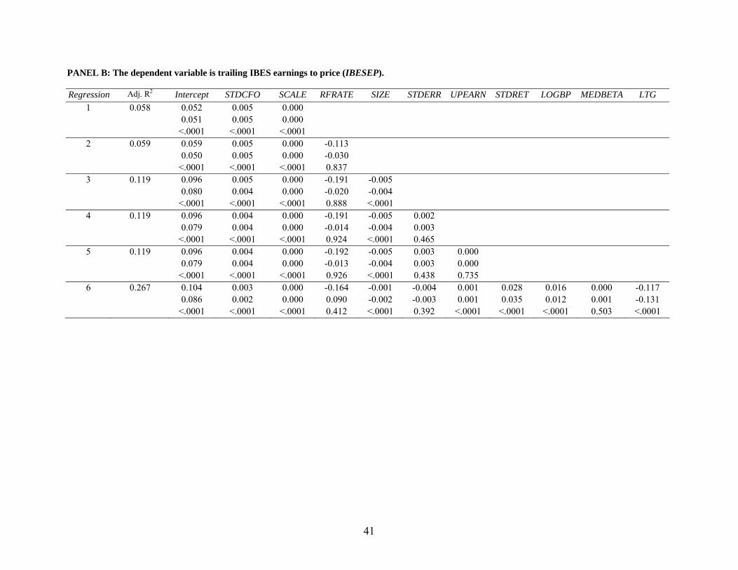
41

PANEL B: The dependent variable is trailing IBES earnings to price (IBESEP). Regression Adj. R2 Intercept STDCFO SCALE RFRATE SIZE STDERR UPEARN STDRET LOGBP MEDBETA LTG

1 0.058 0.052 0.005 0.000 0.051 0.005 0.000 <.0001 <.0001 <.0001

2 0.059 0.059 0.005 0.000 -0.113 0.050 0.005 0.000 -0.030 <.0001 <.0001 <.0001 0.837

3 0.119 0.096 0.005 0.000 -0.191 -0.005 0.080 0.004 0.000 -0.020 -0.004 <.0001 <.0001 <.0001 0.888 <.0001

4 0.119 0.096 0.004 0.000 -0.191 -0.005 0.002 0.079 0.004 0.000 -0.014 -0.004 0.003 <.0001 <.0001 <.0001 0.924 <.0001 0.465

5 0.119 0.096 0.004 0.000 -0.192 -0.005 0.003 0.000 0.079 0.004 0.000 -0.013 -0.004 0.003 0.000 <.0001 <.0001 <.0001 0.926 <.0001 0.438 0.735

6 0.267 0.104 0.003 0.000 -0.164 -0.001 -0.004 0.001 0.028 0.016 0.000 -0.117 0.086 0.002 0.000 0.090 -0.002 -0.003 0.001 0.035 0.012 0.001 -0.131 <.0001 <.0001 <.0001 0.412 <.0001 0.392 <.0001 <.0001 <.0001 0.503 <.0001

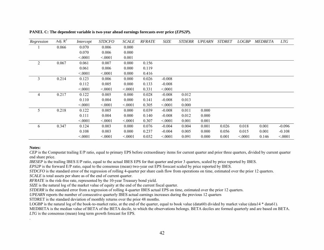
42

PANEL C: The dependent variable is two-year ahead earnings forecasts over price (EPS2P). Regression Adj. R2 Intercept STDCFO SCALE RFRATE SIZE STDERR UPEARN STDRET LOGBP MEDBETA LTG

1 0.066 0.070 0.006 0.000 0.070 0.006 0.000 <.0001 <.0001 0.001

2 0.067 0.061 0.007 0.000 0.156 0.061 0.006 0.000 0.119 <.0001 <.0001 0.000 0.416

3 0.214 0.123 0.006 0.000 0.026 -0.008 0.112 0.005 0.000 0.133 -0.008 <.0001 <.0001 <.0001 0.331 <.0001

4 0.217 0.122 0.005 0.000 0.028 -0.008 0.012 0.110 0.004 0.000 0.141 -0.008 0.013 <.0001 <.0001 <.0001 0.305 <.0001 0.000

5 0.218 0.122 0.005 0.000 0.039 -0.008 0.011 0.000 0.111 0.004 0.000 0.140 -0.008 0.012 0.000 <.0001 <.0001 <.0001 0.307 <.0001 0.001 0.001

6 0.347 0.124 0.003 0.000 0.076 -0.004 0.004 0.001 0.026 0.018 0.001 -0.096 0.108 0.003 0.000 0.237 -0.004 0.005 0.000 0.056 0.015 0.001 -0.108 <.0001 <.0001 <.0001 0.032 <.0001 0.091 0.000 0.001 <.0001 0.146 <.0001

Notes: CEP is the Compustat trailing E/P ratio, equal to primary EPS before extraordinary items for current quarter and prior three quarters, divided by current quarter end share price. IBESEP is the trailing IBES E/P ratio, equal to the actual IBES EPS for that quarter and prior 3 quarters, scaled by price reported by IBES. EPS2P is the forward E/P ratio, equal to the consensus (mean) two-year out EPS forecast scaled by price reported by IBES. STDCFO is the standard error of the regression of rolling 4-quarter per share cash flow from operations on time, estimated over the prior 12 quarters. SCALE is total assets per share as of the end of current quarter. RFRATE is the risk-free rate, represented by the 10-year Treasury bond yield. SIZE is the natural log of the market value of equity at the end of the current fiscal quarter. STDERR is the standard error from a regression of rolling 4-quarter IBES actual EPS on time, estimated over the prior 12 quarters. UPEARN reports the number of consecutive quarterly IBES actual earnings increases during the previous 12 quarters STDRET is the standard deviation of monthly returns over the prior 48 months. LOGBP is the natural log of the book-to-market ratio, at the end of the quarter, equal to book value (data60) divided by market value (data14 * data61). MEDBETA is the median value of BETA of the BETA decile, to which the observations belongs. BETA deciles are formed quarterly and are based on BETA. LTG is the consensus (mean) long term growth forecast for EPS. .

43

Table 7 Regression of growth and risk (the two determinants of E/P) on reported earnings volatility and cash flow

volatility (41,348 firm-quarters from 1992:I to 2002: IV) The first row in each cell is the coefficient estimate for the pooled regression, and the second (third) row in each cell is the mean coefficient estimate (p-value from two-tailed Newey-West test) from regressions estimated each fiscal quarter. PANEL A: The dependent variable is EPS growth forecasts (LTG).

Adj. R2 Intercept STDERR STDCFO SIZE UPEARN 0.052 0.180 -0.026 -0.010

0.179 -0.026 -0.010 <.0001 <.0001 <.0001

0.060 0.204 -0.026 -0.010 -0.003 0.208 -0.025 -0.010 -0.004 <.0001 <.0001 <.0001 <.0001

0.078 0.197 -0.016 -0.010 -0.004 0.002 0.202 -0.015 -0.010 -0.005 0.003 <.0001 <.0001 <.0001 <.0001 <.0001

PANEL B: The dependent variable is market model BETA.

Adj. R2 Intercept STDERR STDCFO SIZE UPEARN 0.010 0.815 0.275 -0.049

0.807 0.320 -0.048 <.0001 <.0001 <.0001

0.063 1.407 0.281 -0.048 -0.088 1.401 0.323 -0.045 -0.088 <.0001 <.0001 <.0001 <.0001

0.064 1.391 0.308 -0.048 -0.089 0.006 1.392 0.338 -0.044 -0.091 0.004 <.0001 <.0001 <.0001 <.0001 0.277

44

PANEL C: The dependent variable is standard deviation of prior period returns (STDRET).

Adj. R2 Intercept STDERR STDCFO SIZE UPEARN 0.020 0.119 0.037 -0.006

0.118 0.032 -0.006 <.0001 <.0001 <.0001

0.093 0.181 0.037 -0.006 -0.009 0.191 0.032 -0.005 -0.011 <.0001 <.0001 <.0001 <.0001

0.094 0.182 0.036 -0.006 -0.009 0.000 0.190 0.034 -0.005 -0.011 0.000 <.0001 <.0001 <.0001 <.0001 0.001

PANEL D: The dependent variable is logarithm of book-to-price (LOGBP). Adj. R2 Intercept STDERR STDCFO SIZE UPEARN 0.084 -1.126 0.429 0.118

-1.121 0.426 0.117 <.0001 <.0001 <.0001

0.349 0.288 0.442 0.122 -0.209 0.248 0.435 0.120 -0.202 0.002 <.0001 <.0001 <.0001

0.383 0.373 0.300 0.122 -0.201 -0.031 0.325 0.293 0.119 -0.192 -0.032 0.000 <.0001 <.0001 <.0001 <.0001

Notes: LTG is the consensus (mean) long term growth forecast for EPS. BETA is a measure of systematic risk calculated by estimating the market model over the prior 36 months. STDRET is the standard deviation of previous 48 months’ returns. LOGBP is the natural log of the ratio of book value to market value of equity, at the end of the current fiscal quarter. STDERR is the standard error from a regression of rolling 4-quarter IBES actual EPS on time, estimated over the prior 12 quarters. STDCFO is the standard error of the regression of rolling 4-quarter per share cash flow from operations on time, estimated over the prior 12 quarters. SIZE is the natural log of the market value of equity at the end of the current fiscal quarter. UPEARN reports the number of consecutive quarterly IBES actual earnings increases during the previous 12 quarters

45

References

Barth, M, J. Elliott and M. Finn, 1999. Market rewards associated with patterns of increasing earnings, Journal of Accounting Research 37: 387-413.

Barth, M., S. Kallapur. 1996. The effects of cross-sectional scale differences on regression results in empirical accounting research, Contemporary Accounting Review13: 527-67.

Beaver, W. and D. Morse. 1978. What Determines Price-Earnings Ratios? Financial Analysts Journal, 34 (4): 65-76.

Chaney, P.K., and C.M. Lewis, 1995, Earnings management and firm valuation under asymmetric information, Journal of Corporate Finance: Contracting, Governance and Organization 1: 319-345

Fama, E., and K. French. 1992. The Cross-section of Expected Stock Returns. Journal of Finance 47 (June): 427-464.

Fairfield, P.M., 1994. P/E, P/B and the present value of future dividends. Financial Analysts Journal, 50(4): 23-31.

Fox, J. 2002. America’s most desired: What's so great about GE? Fortune. 145 (5): 64-7.

Gordon, M.J., 1962, The investment, financing and valuation of the corporation, Richard D. Irwin, Homewood, IL.

Greenspan, A., 1997. Monetary Policy Report to Congress Pursuant to the Full Employment & Balanced Growth Act of 1998, Superintendent of Documents, July 22, 1997.

Hunt, A, S. Moyer and T. Shevlin, 2000, Earnings volatility, earnings management and equity value. Working paper, University of Washington, WA.

Jones, J. 1991. Earnings Management During Import Relief Investigations. Journal of Accounting Research: 29 (Autumn): 193-228.

Kirschenheiter, M. and N. Melumad, 2001, Can “big bath” and earnings smoothing co-exist as equilibrium financial reporting strategies? Journal of Accounting Research; 40(3) 761-96.

Liu, J., and J. Thomas, 2000, Stock returns and accounting earnings Journal of Accounting Research. 38 (Spring): 71-101.

Molodovsky, N. 1953. A theory of price-earnings ratios. Financial Analysts Journal. (November): 65-80.

Myers, L.A. and D.J. Skinner. 1999. Earnings momentum and earnings management. Working paper, University of Michigan.

Newey, Whitney K., and Kenneth D. West, 1987, A simple, positive semi-definite, heteroskedasticity and autocorrelation consistent covariance matrix, Econometrica 55, 703-708.

Penman, Stephen H. 1996. The articulation of price-earnings ratios and market-t-book ratios and the evaluation of growth. Journal of Accounting Research; 34 (2): 235-259.

Preinreich, G.A.D. 1938. Annual survey of economic theory; the theory of depreciation. Econometrica. 6(3): 219-41.

46

Ronen, J. and S. Sadan, 1981, Smoothing income numbers: objectives, means and implications (Addison-Wesley, Reading, MA).

M. R. Sankar and K.R. Subramanyam, 2001. Reporting discretion and private information communication through earnings. Journal of Accounting Research; 39 (2): 365-86.

Skinner, D.J. and R.G. Sloan, 2002. Earnings surprises, growth expectations and stock returns, or, Don't let an earnings torpedo sink your portfolio. Review of Accounting Studies; 7 (2-3): 289-312.

Smith, R., Lipin, S., Maj, A., 1994. How General Electric damps fluctuations in its annual earnings. Wall Street Journal, 3, November, A-1.

Subramanyam, K.R., 1996. The pricing of discretionary accruals. Journal of Accounting & Economics; 22: 250-81.

Thomas, J.K. and X.J. Zhang, 2000. Identifying unexpected accruals: a comparison of current approaches, Journal of Accounting and Public Policy, 19 (4-5): 347-76.

Watts, R. and R. Leftwich. 1977, The time-series of annual accounting earnings, Journal of Accounting Research 15: 253-71.

Zarowin, P. 1990. What determines earnings-price ratios: revisited. Journal of Accounting, Auditing, and Finance 5 (3): 439-57.