teletraffic in the kenyan network-overview assesment and
TRANSCRIPT

!!
u TELETRAFFIC IN THE KENYAN NETWORK --OVERVIEW ASSESSMENT AND FORECAST
Kris
S T r V
M 7 rr 'N u ' - l is r i v
Elizabeth Lusi .Migwalla, B.Sc. (Eng.)
A thesis submitted in part fullfilment for the Degree of Master of Science in Engineering in the
f .^University of NairobiTj
1985
UNIVERSITY o f NAIROB! l ib r a r y

This thesis is my original work and has not been presented for a degree in any other University.
ELIZABETH L. MIGWALLA
This thesis has been submitted for examination with my approval as a University supervisor.
MR. M. 0. ADONGO
Ill
ACKNOWLEDGEMENTS
The author is greatly indebted to Mr. M. 0. Adongo and Dr. P. C. Egau for their advice and encouragement during the preparation of this work. Further acknowledgements go to members of the KP‘ & TC who assisted in the collection of the
data presented in this thesis.
Many thanks are due to Mrs. Phyllis M. Njihia and Mrs. Sophie A. Onyango for the quick and accurate typing of the manuscript.
Finally to Ayub, Sheba and Marjorie - thank you for the patience and understanding.
1
IV
ABSTRACT\
A telecommunications network is an orderly, economical arrangement of telecommunications plant
which allows the transmission of information by electrical means. Two objectives of any network are^ to provide a good grade of service and to avail service to new users with minimal delay.
This thesis gives an overview of the Kenyan Telecommunications network and introduces its structure and the services it offers. By subdividing the network into smaller networks evolved around the major
towns, the extent to which the network objectives are met is assessed. A simple systematic method of obtaining forecasts on future service demands is presented.
The estimates of the offered grades of service show that 24% of the links connecting automatic switching systems offer worse grades of service than the designed numerical value.
< Further results show that for the automated network around the major towns in Kenya the demand for telecommunications service has not been met. A significant percentage of what is considered

V
1 total demand’ is contributed by waiting users. The fact that this unsatisfied demand figure tends to increase with time leads to the conclusion that demand forecasts ma y have not always been reliable.
The methods deviced in this thesis would be useful for telecommunications organizations whose developing networks do not incorporate advanced network management facilities.
/
*V'
1
CONTENTS
Page
DECLARATION------------------------------ iiiACKNOWLEDGEMENTS ------------------------- iiiABSTRACT---- -----------------------------. ivList of Abbreviations and Symbols------ - - xCHAPTER ONE. INTRODUCTION -------------- 1CHAPTER TWO. AN OVERVIEW OF THE KENYAN
TELECOMMUNICATIONS NETWORK - 5
2.1 Telecommunications Network ---- 5i
2.1.1. Network Configurations - 62.1.2. Mesh Configuration ------ 72.1.3. Star Configuration ------ 72.1.4. Heirarchical Network ----- 9
. . '2.2 Switching Systems ------------- 10
2.2.1 Basic functions of aiSwitching System -------- 11
2.2.2. Functional Elements of the.'*• Switching System--------- 13
2.3 Switching Systems in Kenya---- 15
• y 2.3.1. ' Manual Exchanges------ -- 162.3.2. Step-by-Step Electromechanical
Exchange ---------------- • 182.3.3. Crossbar Switching Systems-- 18

V l l
2.4 The Kenya TelecommunicationsNetwork Heirarchy ----------- 21
CHAPTER THREE. TELECOMMUNICATION TRAFFIC INKENYA - MEASUREMENTS --- 24
3.1 -Traffic Measurements -------- 303.1.1 Traffic Intensity
Measurements ----------- 303.1.2 Traffic Intensity
Measurements in Crossbar Exchange--------------- 33
3.1.3 Traffic MeasuringEquipment -------------- 36
3.1.4 Traffic Intensity Measurements
in Manually operatedExchanges -------------- 40
3.2 Practical Measurements andResults --------------------- 47
3.2.1 Observation of Traffic _Data--------------- 49
3.2.2 Results------------ 54
CHAPTER FOUR. -&RADE OF SERVICE ON/ c TELECOMMUNICATIONS LINKS--- 614.1 Traffic Theory Models -------- 63
4.1.1 Pure Chance Traffic ---- 644.1.2 Erlang loss Model-- 64

V I 11
4.1.3 Engset Distribution Model --- 65
4.2 Computer Programme "ERLANG B" ---- 664.3 Results -------------------------- 69
4.3.1 Coast Network-------------- 784.3.2 Nakuru Network------------- 78
4.3.3 Kisumu Network------------- 794.3.4 Nyeri Network------------- 804.3.5 Nairobi Network------------ 80
4.4 High Usage Routes--------------- 81
4.5 Comparison of Conventional Methods of obtaining AQ with the 'Erlang B*Programme--------- -------------- 82
CHAPTER FIVE. DEMAND FORECASTS ------------- 85
5.1 Assessment of the Network forUnsatisfied demand -------------- 86
5.1.1 Data Presentation---------- 875.1.2 Observations rrom the Data
and Plots -------------- 1005.1.3 Choice of Model for the growth \-w of Demand for Telecommunications
• Service -------------------- 103*5.2 Determination of Growth Rate ---- 112s
5.2.1 Computer Programme - LeastSquare Regression ---------- 113
1

IX
5.2.3 Results and Observations -- 121i
5.3 Forecasting of Demand forTelecommunications Service ----- 127
;
5.3.1 Forecasting Methods ------- 1275.3.1.1 Trend Methods -------- 1285.3.1.2 Comparison Method ---- 132
CHAPTER SIX. CONCLUDING COMMENTS --------- 135
Appendix I. METHOD OF LEAST SQUARES ------ 141
REFERENCES------------------ r-------------- 147
c
1

X
I(t)A
Ao
AcE
BNSCASC
GSCEO
RS.
C
N
V
SRGOSnNft) ;y R(t) ;A2 k
MFC
1
LIST OF ABBREVIATIONS AND SYMBOLS
Volume of trafficTraffic Intensity at time t
Traffic intensity in ErlangsOffered traffic intensity in erlangsCarried traffic intensity in erlangsTime congestionCall congestionNational Switching CentreArea Switching CentreGroup Switching CentreEnd Office
Rotary SwitchNumber of meter operationsNumber of Scans'Send' Signalling wire‘Receive’ Signalling wireGrade of serviceNumber of circuits in a routeDemandGrowth rateSaturation value for Logistic growth Multi-Frequency Compelled
curve

1
CHAPTER ONE
INTRODUCTION
The first stage in the development of any
area is the provision of a complete infrastructure including power, water and communication. Telecommunication service is an essential tool in the achievement of development.
In Kenya the provision of telecommunications services is a monopoly of the Kenya Posts and Telecommunications Corporation (KP & TC), whose telecommunications network can be considered as one of
the more advanced in Africa. It offers a variety of services such as telephone services, telex services, data transmission services and facsimile services. International Subscriber Dialling services have been recently introduced. Systems employing latest technologies are incorporated in the network such as digital microwave radio systems and PCM systems on cable. Future plans include the introduction of digital public switching systems, optical fibre
transmission systems as well as public land mobile telephone servic^.
A network such as this has the objective of providing services to the satisfaction of the public.

2
However, it is not uncommon to hear complaints, for
example "I applied for a telephone two years ago and have not been served to date” or "In the morning hours it is impossible to call a number in Kisumu from Nairobi".
In advanced networks employing digital techniques, incorporated network management facilities perform continuous traffic observation duties to monitor traffic flow characteristics. The Kenyan network is predominantly analogue and relies on manually collected and processed data for its network management. Traffic Tables derived from similar tables previously used in other (developed) countries,
particularly Japan and Sweden are used when observing and processing teletraffic data. However in some cases these methods and tables may not appropriately represent the Kenyan network status as calling habits are dictated to a large extent by culture, and differ from country to country. As an example, in Kenya it is observed that the holding times aremuch longer than^ those observed in developed
•J V'countries. This is because whereas, for example, the
Japanese use the telephone for short messages,Kenyans have.aytendency to hold long social conversations on the telephone. In Kenya a business

3
/
conversation only begins after words of greetings and enquiries about the familyl
Demand forecasting is performed in two categories:-
forecasting in new areas where service is to
be introducedforecasting for growth in areas already having service.
In the first case a physical survey of the area tobe served is done, where personnel travel from houseto house enquiring from the inhabitants whether or
not telephone service would be required. In additionbuilding types are graded into those likely andthose not likely to require service.In the second case it has been the practice toforecast demand by judgement. By looking at theconnected users’ figures and the figures of theunsatisfied demand in an area, a forecast of futuredemands is'made intuitively. The guideline for theforecaster is that the unsatisfied demand figure
*shouj/d reduce whrie the connected lines should increaseThis method is dependent on the experience of theforecaster and may sometimes result in an ill-
1dimensioned route.

4
This thesis is an attempt to explain why for example the time lag between application for and provision of service is sometimes long. It gives reasons why it is difficult to communicate between some points in the network and identifies those points.
Simple techniques of teletraffic data processing are evolved. In particular a simple programme to derive estimates of the blocking encountered on transmission links is developed.
a sound data base and is not dependent on the individual forecaster, and is thus more reliable.
Also a procedure for estimating demand forecasts is established. This procedure depends on
• /
\

5
CHAPTER TWO
AN OVERVIEW OF THE KENYA TELECOMMUNICATIONS NETWORK
2.1 Telecommunications Network
The object of a telecommunications system is to transmit information by electrical means between points connected on it. A permanent connection provided between each terminal to every other
terminal in the system would not only be prohibitively expensive, but would result in a lot of confusion caused by the large number of wires that would have to be used. To a^oid this expense and confusion it is found necessary tc provide common switching points to which terminals are connected each by a pair of wires; and to interconnect these common switching points by interexchange links and transit
. switching points. This arrangement constitutes a
telecommunications network.
A telecommunications network is thus defined as a method of connecting switching points so that any terminal can communicate with any other terminal. Basically the network can be decomposed into two parts.
1

6
Network
11Transmission System
Figure 2.1: Telecommunications Networki - . .
The ideal transmission system - allows any two users (connected to any two terminals) to communicate satisfactorily, while the switching systems permit economical building of the network by concentration of transmission facilities. Viewed in this way the network can be illustrated a’s a system of nodes interconnected by links. The nodes represent switching systems; and the links represent circuit
groups which carry traffic between the nodes. Eac^1 node can act as a traffic source, a traffic sink or a transit point, and a link may either be unidirectional or bidirectional.
2.1.1 Network Configurations
By way t>f introduction consider a case whe r e
userSy have access^to the network by a local switch^11? c
system (or node) to which they are connected. Tf>e problem to be solved then is that of interconnecting all these nodes to allow communication between e^-c^
" lSwitchingSystem

7
user to any other user at minimum cost, with maximum efficiency. Basically there are two methodsI iof interconnection that can be devised:-
•
- mesh connection- star connection
2.1.2 Mesh Configuration
In mesh connection every node in the system
is connected to every other node by a direct link.
Figure 2.2: Mesh Configuration
With this configuration the number of links ’ L' is related to the number of nodes fn’ by the equation
L = n(n-l)/2 ' ~
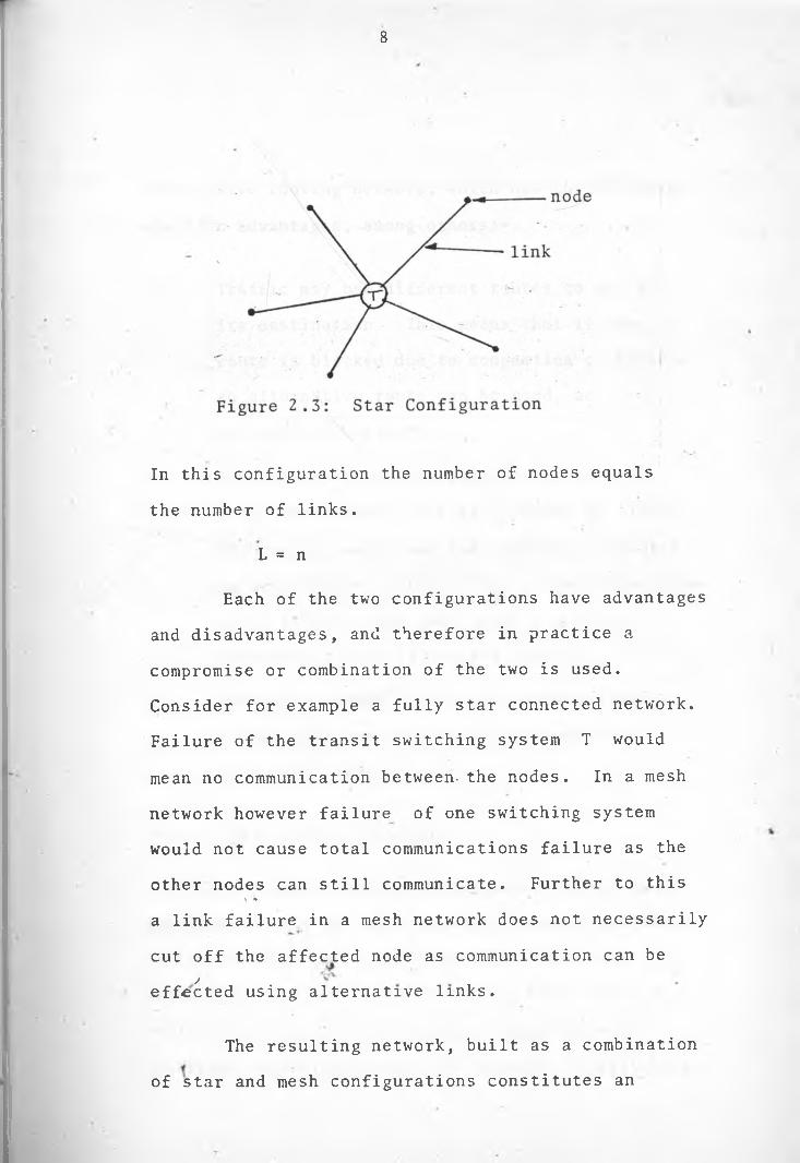
2.1.3 Star Configuration
* . „ . . .• j A star connection utilizes an interveningc .
(transit) point T so that each node in the system is interconnected to any other via this transit switch.
8
In this configuration the number of nodes equals the number of links.
L = n
Each of the two configurations have advantagesand disadvantages, and therefore in practice acompromise or combination of the two is used.Consider for example a fully star connected network.Failure of the transit switching system T wouldmean no communication between- the nodes. In a meshnetwork however failure of one switching systemwould not cause total communications failure as theother nodes can still communicate. Further to this \ *a link failure in a mesh network does not necessarilycut off the affected node as communication can be
jeffected using alternative links.
The resulting network, built as a combination of star and mesh configurations constitutes an

9
alternative routing network, which has the following
specific advantages, among others1/i' .
1) Traffic may use different routes to get to its destination. This means that if one route is blocked due to congestion or failure an alternative route can be used, and thusno traffic is ‘lost'.
2) The efficiency of the network is enhanced since the traffic is first offered to direct
high usage routes and the overflows directedto alternative routes. These alternative routes carry traffic from many origins and are therefore also utilized efficiently.
3) There is a trade off on costs where direct routes can save on the transit switching equipment costs.
2.1.4. Heirarchical Network
In order to reduce the number of links to a reasonable value and also permit efficient handling of high traffic intensities on busy routes and
■ yoverflows a heirarchical network is called for. A
heirarchicalnetwork has levels of importance of exchanges which constitute the network. A switching

10
system depends on the next (higher,) order system in the heirarchy to enter the network. There are two connection methods that can be adopted by automatic switching systems namely:-
direct connecting method indirect connecting method.
In the direct connecting method the switching
equipment responds to the respective digits dialled by the caller, operates in sequence to locate the called terminal and establish the connection as soon as the last digit is dialled. In the indirect connecting method the equipment receives and memorizes all dialled digits, and converts these digital codes into other codes necessary for the identification of the called terminal. The connection of the path is then performed by the switch.
2.2 Switching Systems
Having briefly discussed the telecommunicationsnetwork as* a whole a closer look at the switchingpart of the network follows with particular referenceto the switching Systems in the Kenyan network, togive an overview and appreciation of the basic conceptof telecommunication switching,
ti

11
The important point of the switching operation is to select desired equipment and connect the calling party to the desired party. Lines connected
i \ *
to one switching point (node) are divided into two groups: Inlet group and outlet group. In the inletgroup calls are originated by users, who declare their intention for speech. An originated call from the inlet group is connected to the outlet group which is divided into several indepedent sections, each serving a similar purpose.
Telephone switching systems are classified into two groups: manual switching systems andautomatic switching systems. The basic functions are common to both system groups; with connections being completed by operators in manual systems while in the automatic systems the connections are automatically established by the switching equipment.
2.2.1 Basic functions of a Switching System
The.re are eight basic functions of a switching system necessary to achieve switching operation as discussed above:-
Alerting AttendingControl

12
4. Information receiving5. • Busy testing6. Interconnecting7. Information transmitting
8. Supervisory.
When a user seeks to establish a link for communication the switching system is alerted (1). There has to be some communication from the switching system to the user to the effect that the request for the establishment of a link is being attended to (2).
The user then gives information as to which other point in the network he requires to communicate with. This information is received by the switch; which then tests for the possibility of establishing the connection; and informs the caller if the connection cannot be established. One of the reasons leading to failure of a required connection is a busy link encountered along the path of connection. Thus this condition must be tested by the switching
system; and if the busy test is negative the system goes ahead to^make the required connection and informs the calling user that the connection has beeft made successfully. The required link for speech having been thus established the calling party communicates with the required party.

13
The duties performed by the switching system do not end at this point; for it must supervise the established connection such that when the use of the established link is completed it can release all the connections; thus rendering the path free
for use by other callers.
2.2.2 Functional Elements of the Switching System
In order to perform the functions outlined
above efficiently the switching system has necessarily
three functional elements:-
- Concentration- Distribution- Expansion.
The concentration stage reduces the number of switching paths and trunks.In the distribution stage traffic is channeled to the respective routes.The expansion stage allows access to incoming
circuits vfor all the users connected to the terminals
efficiently.„ *J - v*
For illustrative purposes consider a switching system as having originating-line appearances where callers requiring to be connected are accessed; and terminating-line appearances where users to

14
•/whom communication is required are accessed. This idea is illustrated in Fig. 2.4. belowi/ TRUNKS TO/FROM
OTHER SWITCHING SYSTEMS
ORIGINATINGCONNECTIONS
BCONCENTRATION DISTRIBUTION
TERMINATINGCONNECTIONS
EXPANSION
Figure 2.4: Functional Elements of a Switching System
For any local switching system there are three different call possibilities, namely:-
a) Intra-system call where a caller connected onthe switching system wishes to communicate with another user also connected to the same system. The routes used in this type of call
are
A ---- B--- - C----- D ----**E.
b) Outgoing connection where an originatingcaller connected on the switching system
. J ^c wishes to communicate with another user
connected on a different local switch. The routes required in this kind of connection
A ~Fare B

15
c) Incoming connection where it is required tocommunicate with a user on a local switch,
from a distant switching system. The relevant routes here are G --► D — —
Call concentration occurs at B and call expansion takes place at D; whereas distribution takes place at C in this illustration.
2.3 Switching Systems in the Kenyan Network
In the Kenyan network both manual and automatic switching systems exist. From an approximate 9^,000 users (telephone connections) approximately
78.000 are connected to automatic exchanges and12.000 connected to manual exchanges. This represents 871.of the total connection being served by automatic systems and 13% being served by manual boards.
The automatic switching systems are of two. main types, namely the Strowger step-by-step
electromechanical exchange and the Hitachi Crossbar electromechanical exchanges. However the step- by-step systems a*re old and relatively few; and are earmarked for replacement by the next generation of switching systems in the near future.
t

16
The manual exchanges in existence in the network are of two capacities; one being a 70-linemagneto switchboard and the other a 100-line magneto
!switchboard. These two switchboards form the
building blocks of manual exchanges as for example two 70-line switchboards can be combined to serve 140 users; or where 400 users are to be served four 100-line switchboards can be used. Generally manual exchanges are provided in remote locations where the demand for telephone service is below 500 users. They are linked to 'parent' exchanges which are normally automatic exchanges, and depend on these 'parent' exchanges for access to the rest
of the network.
Following is a brief description of the switching operation in each of these exchange types.
2.3.1 Manual Exchanges
In a typical manual switching centre the operator performs all of the eight switching functions. The interconnecting function is done
via jacks which appear in front of the operator.' X x* XThefe are jacks for users lines and jacks for
outgoing and incoming circuits or trunks, which link the^switch to other distant exchanges. These jacks are interconnected by use of connection cords. The

17
number of connection cords is always less than half the number of jacks; and the concentration stage is thus accomplished at this point. Distribution is also considered to take place at this point since any cord may be used to complete a connection to any of the terminating jacks. The attending- alerting functions are accomplished as follows:A user alerts the exchange by generating a 17 Hz
sinusoidal signal from his receiver instrument set. This signal causes a mechanical indicator to drop, thus drawing the attention of the operator to the demand for service. •
Next the operator assumes the control function determining which connection cords are idle; using
one of these idle cords to speak to the calling user; obtaining information from the caller regarding the party with which a connection is sought, determining which outgoing jack should be used; testing the selected link for busy condition and eventually making the connection. The called party is allerted by a signal which rings his telephone instrument bell; and a communication channel is thus established. The operator supervises the connection and releases all the equipment when the communication is terminated.
1

f
18
2.3.2 Step-by-step Electromechanical Exchange
The few step-by-step exchanges still in existence in the Kenyan network are situated in Nairobi, Mombasa, Nakuru and Kisumu.
!/
/ A step-by-step exchange is based on rotary ortwo-motion switches each provided with an exclusivelyused control circuit. These control circuits control vertical or horizontal motion upon receipt of dial pulses. Each two-motion switch has 10 levels. In its simplest form dial pulses from the users’ telephone activate the switch, with each pulse causing the switch to step by one level. The step-by-step
exchange therefore adopts the direct connecting method. ' .
2.3.3 Crossbar Switching Systems
a speech path under common control equipment. Commoncontrol is here defined as providing a means of
\ .control of the interconnecting switch network, first identifying the input and output terminals of the
• l
The crossbar is a matrix switch used to establish
net^6rk that are "free and then establishing a path between them.

19
In this section the operation of the Hitachi crossbar exchange will be outlined. However it must
be pointed out that there are other types of crossbar exchanges in the network which will not be discussed as they exist in negligible numbers.
Figure 2.5 Shows the arrangement of the whole cross-
Figure 2.5: Crossbar Exchange
The speech circuit is a crossbar switch network where
the^switching operation is performed. The register is a circuit wrhich memorizes digits received by it. The number group is a translation circuit which deter mines the corresponding terminal location from a
dialed number

20
The connection circuits perform inter-equipment connections for individual steps of the switching operation. In the crossbar switching system the
control circuits are centralized in one section which makes it possible to have uniform control operation for the whole switching system. A description of the control operations performed by the common control
circuit follows.
When a calling user lifts the handset of the
telephone instrument, the common control circuit detect the originating condition and starts operating by connecting the calling line to a free register. The register thus connected transmits a dial tone to the calling user. When the caller dials the desired number the dialled digits are stored in the register. During the period when dialled digits are being transmitted to the register the common control circuit is released from the calling line and is free to
serve other calling users. The common control circuit is seized again as soon as the number of digits required for the connection have been stored in the register. The common control circuit identifies theodesired line based upon the received digits, using the number group (translation circuit) and performs the required connection operations on the crossbar switch network.

21
y .2.4 The Kenyan Telecommunications Network Heirarchy
Figure 2.6 is a representation of the portion of the Kenyan network in which the traffic data processed in this project was obtained. On it is
represented the automatic switching systems of the crossbar types (as nodes) and the circuit groups (links) connecting the switches. It is basically a heirarchial network with the lowest ranking switch designated ’end office' and the highest ranking switch known as the national switching centre,. (see
Fig. 2.6a)..’
There is one National switching centre situated - in Nairobi, which also performs the duties of an area switching centre for Nairobi. Other area switching centres are situated in Nyeri, Kisumu and Nakuru. In Mombasa a group switching centre performs the functions of an area switching centre for the area.The other group switching centres are situated in major towns such as Kericho, Eldoret, Kakamega,
Malindi, Machakos, Athi River, Thika, Nanyuki, Muranga, Nyeri, Meru and Embu.
> .<L
t

Figure 2.6: Kenyan Te "
(Automatic Switch11'
‘U | \ / ' ' / t f
/ // f'
^ \ v / 7 /
, OKj IrMV'u

23
Highest Rank
A□
Lowest Rank O
Figure 2.6a: Heirarchy oin Kenya
National Switching Centre
Area Switching Centre
«Group Switching Centre
End Office
Switching Systems
1
24
CHAPTER THREE
TELECOMMUNICATIONS TRAFFIC IN KENYA - MEASUREMENTS
In chapter 2 the telecommunications net work was reviewed with a view to introducing
the various services that are offered by it.To provide a communications service of this nature at a reasonable cost the network should necessarily be designed such that it satisfies the communications needs of the users; but does so with just the amount of switching equipment and transmission plant necessary to meet a specified standard of service. In order to accomplish this the
network designers must have access to certain vital information.
In a general planning and installation cycle of a telecommunications network there are seven basic activities which are undertaken as Fi-g. 1 .1 illustrates.
*
1

25
TRAFFIC TRAFFIC DATA TRAFFICMEASUREMENTS PROCESSING FORECASTING
EQUIPMENT WORKS GROUP,INSTALLATION PROGRAMME DIMENSIONING
— _ - . »• i?. ---- ...
Fig. 3.1: Typical Planning and installationcycle of a Telecommunications network.
As can be appreciated five out of the seven activities involve traffic engineering. Before the network designer can effectively accomplish his objective of evolving an efficient network he must know the traffic' intensities offered by each group of subscribers to every other group. He must have some idea of the
characteristics of the traffic flows and the effect of splitting or merging them from point to point in the network. This information is obtained by me^ns of collection and analysis Of traffic data. This data is then used to forecast future traffic growth and forms the basis for.network dimensioning. Any network

26
congestion is monitored from this collected and analysed data.
This chapter deals with telecommunication traffic in Kenya and to begin with some important parameters are introduced below:
Telecommunications Traffic refers to the aggregate of communication messages carried between two or more points in a telecommunications network.
The traffic intensity on a group ofcircuits or devices is dependent on the total numberof messages in progress simultaneously. The unitof traffic is the 'erlang' which is dimensionless.One erlang of traffic represents one occupied circuit
carrying a telecommunications message. To put itanother way one erlang of traffic intensity on onetraffic circuit represents continuous occupancy ofthat circuit. When considering a group of circuitstherefore, the traffic intensity in erlangs is the \ ♦number of "call seconds per second" or the number of "call hours per^hour".
- V'
For planning and dimensioning purposes it
is mqre meaningful to consider the average

27
rather than instantaneous traffic intensity, with the average being computed.over 60 minutes.
The Volume of Traffic is often times refered to and has units of erlang hours. It
is dependent on the number of messages and their duration.
ThusV =
ft ,I(t)dt o
. r where I(t) is
Traffic intensity at time t. , ...... 3.1
The Holding Time . is the duration of the message and consequently the time of occupation of the transmission circuit and switching equipment.
Call arrivals as is suggested gives an idea of the times at which telecommunications messages arrive at a stage in the network.
- ..Consider now traffic flow with the\ %
following characteristics,
(i) holding^times ti 2 ..... tR ; n =number of calls
(ii) duration period under consideration = T1
1
28
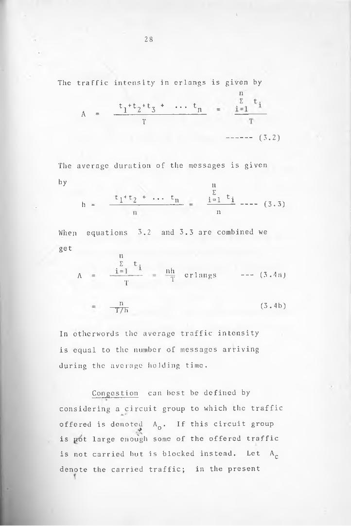
The traffic intensity in erlangs is given byn
A =t +t0+t7 + ... t1 2 3 n
1’(3.2)
The average duration of the messages is given
by
h =t,+to + ... tL1 L2 • * * Ln
niE=i nn
--- (3.3)
Whenget
A
equations 3.2
n
T
and 3.3 are combined we
nhT e r l a n g s — (3.4aj
nT7TT (3.4b)
In otherwords the average traffic intensity is equal to the number of messages arriving during the average holding time.
Congestion can best be defined byconsidering a circuit group to which the trafficoffered is denoted A . If this circuit group
& 0is jrot large enougli some of the offered trafficis not carried but is blocked instead. Let Acdenote the carried traffic; in the present
1
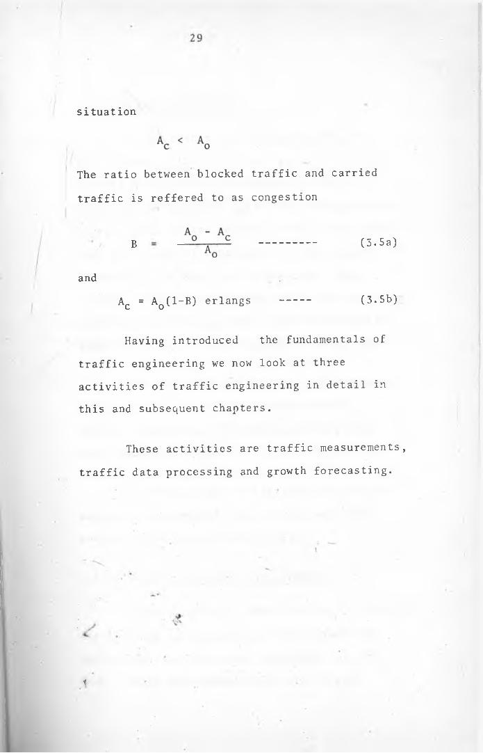
s i t u a t i o n
The ratio between blocked traffic and carried
traffic is reffered to as congestion
Having introduced the fundamentals of traffic engineering we now look at three activities of traffic engineering in detail in this and subsequent chapters.
These activities are traffic measurements, traffic data processing and growth forecasting.
B (3.5a)
andAc = A0(l-B) erlangs (3.5b)
f

30
3.1 TRAFFIC MEASUREMENTS
As has been stated previously traffic in a network is observed for two major reasons. Firstly it provides measurements of data to give information about the traffic being handled at each point in the network. This facilitates easy monitoring of congestion or any unusual
behaviour of systems in the network. Thus secondly it provides information on the necessary supervision of the network so that the required grade of service can be maintained at all times.
The measurements that are most frequently taken are traffic intensity measurements,
traffic dispersion measurements, holding time measurements and grade of service measurements.
For the purposes of this project trafficintensity measurements were taken, and those /are discussed in more detail below.
3.1.1 Traffic Intensity Measurements
Traffic^ intensity measurements are requiredj v* *
*for the long term planning of the network as well as for the day-to-day management of the*same. These measurements are used to give

31
indications as to when an existing switching' , ’ * i
point may need to be extended, and also to assist in the specifications for new exchanges.
Telecommunications traffic is generated by calls or messages arriving in a system (of the network), staying connected for a certain duration (holding time) before disconnection. Thus theoretically it is possible to obtain traffic intensity measurements by simply observing the arrival of each message and its duration. In other words if a group of circuits
is scanned to determine the instantaneous circuit occupancy, data can be obtained from which the carried traffic intensity can be deduced. In practice this data is obtained in one of the following ways:
(i) Scanning periodically and recording
the number of occupied circuits in the group.
^ *>\ *
(ii) Continuously recording the number of occupied circuits of the group.
(iii) Continuously recording and integrating the number of occupied circuits of the
t group.

32
In this project the first method of scanning periodically was adopted, with the result of each scan being the number of occupied circuits X(t) at scan time t;. In chapter 2 it was stated that the bulk of the automatic switching systems in Kenya (at the time when this work was being undertaken) was made up of crossbar exchanges. Further, a look at Fig. 2.6
illustrates the fact that mostiGroup Switching Centres
(GSC’s) are of crossbar types, and for this reason the method used for measuring traffic intensities in crossbar exchanges will be described in detail.As far as possible throughout the traffic measurement exercise, measurements were done at the crossbar exchange end. Thus considering two exchanges A and B for example (Fig. 3.2).
CROSSBAREXCHANGE
A OUTGOING TRAFFIC FROM A --- -------v-----------■INCOMING TRAFFIC TO A
OTHER EXCHANGE
^ Figure 3.2:*v"Connection of two exchanges A and B
1

33
The traffic intensities on both the outgoing route from A and the incoming route from B are measured at A which is a crossbar
/exchange.
i • . ;3.1.2 Traffic Intensity Measurements in
Crossbar Exchange
Crossbar exchanges are common controlled switching systems offering full availability.In the Kenyan network in so far as traffic intensity measurements are concerned the exchanges are grouped into two groups, one group to which the traffic measuring equipment is provided and the other where none is provided.
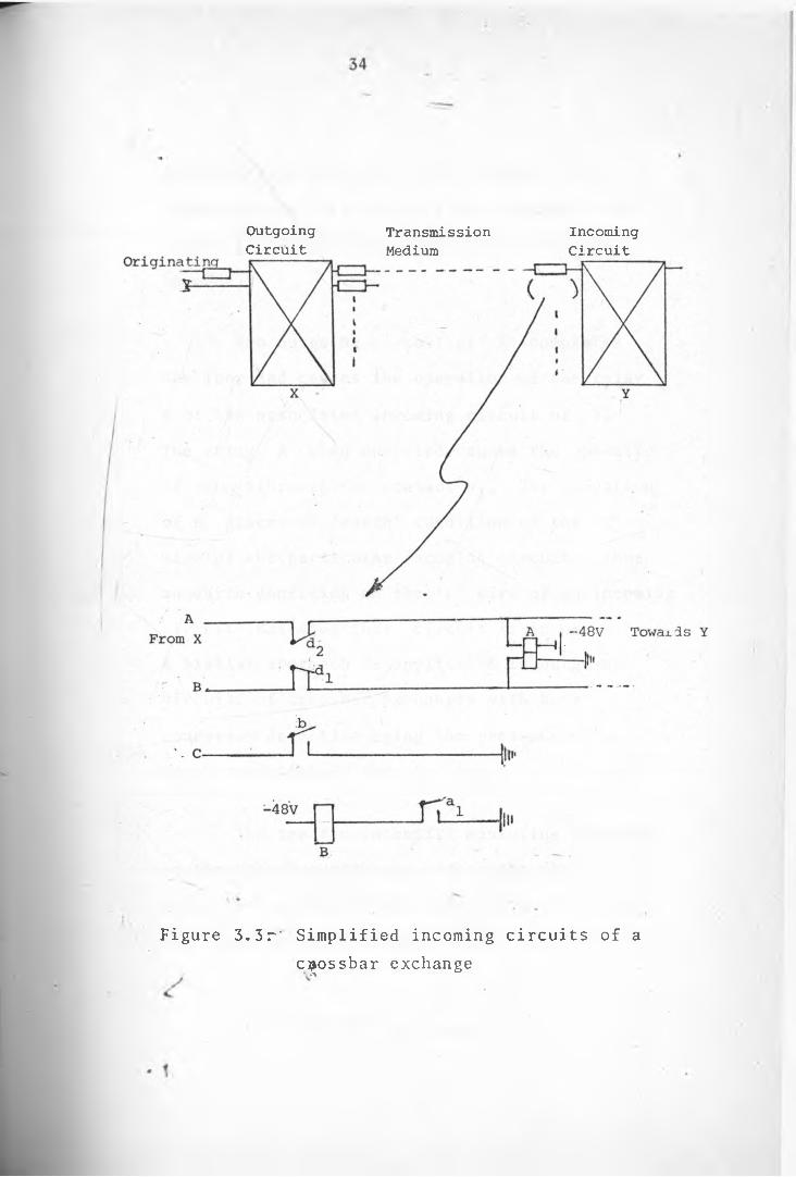
In Fig. 3.3 is illustrated a typical incoming circuit to a crossbar exchange. The circuit is considerably simplified to show only the relevant parts for our purposes.
The arrangement of Fig. 3.3 shows an exchange. X as the originating exchange. The message may^be originated by a subscriber on exchange X; or#if X has transit facilities
y # *
tfre message may be originated from another preceding switch. Y is the receiving exchange,
1
OutgoingCircuit
TransmissionMedium
IncomingCircuit
Figure 3.3r* Simplified incoming circuits of acrossbar exchange

accommodating the subscriber required for communication (This is only one example of the kinds of communication connections that can
be made).
The outgoing circuit of X. completes the loop and causes the operation of the relay
A of the associated incoming circuit of Y.The relay A when operated causes the operation of relay Bthrough the contact a- , The operation of B places an ’earth* condition on the 'C* wire of the particular incoming circuit. Thus an earth condition on the f C' wire of an incoming circuit indicates that circuit is in use.A similar approach is applicable to outgoing circuits of crossbar exchanges with busy
condition detection being the presence of an earth condition on the C wire.
The traffic intensity measuring equipmentin the crossbar exchange adopts the aboveprinciple to detect busy conditions on circuits.Its operation is outlined briefly below.
*: > . . -
C •. , • *D IV ER SIT Y Qp NAIROBI
library
1

36
3.1.3 Traffic Measuring Equipment
This equipment adopts a simultaneous operation measuring method, where the number of busy circuits is counted at predetermined intervals and recorded on a counter.
Figure 3:4 illustrates the trunking diagram to show how the equipment is connected
to the other parts of the exchange.
Figure 3:5 is a diagram illustrating the various components of the equipment and will
» i •
help to give clarity when outlining the operation.
Operation :«
The control (C) wires (previously mentioned) of all circuits for which traffic is
to be measured are led in units of 21 into the SCAN circuit through rotary switches .RSI to RS5. Each rotary switch has facilities to connect 5 circuits except for the fifth switch which connects oilly one circuit. (The rest of the switch is used^for control leads for the equipment). The rotary switches step simultaneously to bring into the scan circuit different groups of (21) circuits each time.

37
IncomingCircuits Exchange Outgoing
Circuits
Traffic Measuring Equipment (TME)
Figure 3.4: Trunking Diagram for the TME\
/c
t
V'
(

38
RSI. RS4 RS5
The scan rotary switch scans the 21 circuits connected to it by the connector rotary'switches (RSI - RS5) every three minutes.A, busy condition on a circuit (an earth conditions
on the C wire) causes an operation of the counter.
1

39
Each meter is dedicated to count the busy conditions (circuit occupancy) for a given
group of circuits.
By scanning a particular group of circuits at three minute intervals and stepping the counter for each busy condition detected the carried traffic in the group can be estimated as follows
Carried traffic Erlangs (3.6a)
where C = Total number of meter operations
N = Number of Scans.
For one hour N = ^ = 20
AcC_20 erlangs (3.6b)
.Ffcr crossbar exchanges without traffic measuring equipment the carried traffic is estimated from ata obtained by manual count.
By observing the 'AT relays (refer to Fig. 3:3) of the circuits in the group, busy

40
circuits are easily identified. The scan is done at intervals of 3 minutes and thus bythe same argument
i!.
^c = "ZU Erlangs.I ^ •
where C = total number of busy counts
3 . 1 * 4 * Traffic Intensity Measurements in Manually operated Exchanges
The heirarchical network arrangement adopted for the Kenyan network makes it necessary in some situations for traffic measurements to be carried out in manual exchanges. Consider once more the network arrangement.
NationalSwitching CentreArea Switching CentreGroup Switching CentreEnd Office
Hot 1 Mo't-i.vr-rV ArranaorrV n t"

41
The NSC and ASC’s are all automatic exchanges; and switch traffic to and from the GSC’s.At the GSC level the switching can be done automatically or manually as is also the case at the E.O level. With this arrangement therefore there are some users who can only be connected to other users through manually operated switches. The table in Fig. 5.7 gives a summary of these connections.
From A To B
(Originating Exchange) (Terminating Exchange)
1.- Manual Manual (Terminating)
2. Manual Manual (Transit)
3. Manual Automatic (Terminating)
4. Manual Automatic (Transit)
5. Automatic Manual (terminating)
6. Automatic Manual (Transit)
\ *Fig. 3.7 Table Summarizing Connections
Requiring Manual Operations
<1 Consider a subscriber connected to a manual end office requiring to communicate with anpther subscriber connected on a different
42
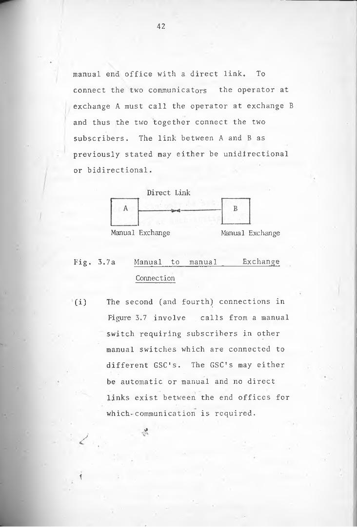
manual end office with a direct link. To connect the two communicators the operator at exchange A must call the operator at exchange B and thus the two together connect the two subscribers. The link between A and B as previously stated may either be unidirectional or bidirectional.
Direct Link
Manual Exchange Manual Exchange
Fig. 3.7a Manual to manual_____ ExchangeConnection
(i) The second (and fourth) connections in Figure 3.7 involve calls from a manual switch requiring subscribers in other manual switches which are connected to different GSC‘s. The GSC’s may either be automatic or manual and no direct links exist between the end offices for which-communication is required.
*y
1

43
As an example consider the arrangement
in Fig. 3.7b.
A B c____ _____________
Manual Exchange -Manual Exchange (2) . Manual Exchangeor Automatic Exchange (4)
Figure 3.7b: Manual - Auto - Manual Exchange ConnectionThese connections can only be set up by involving operators at each station. For this
reason.there are manual boards even at automatic switching centres and they serve as the only facility for connecting subscribers connected on manual exchanges.
(ii) Cases 5 and 6 involve automatic exchanges requiring to communicate with subscribers
on manual exchange areas. Once again this is only possible by manual switching
- at both ends of the communicating links vand necessitates - the provision of manual operation facilities even in automatic switching centres.
• <r" •
Thus traffic measurements in manual . fexchanges play an important role in assessing
teletraffic characteristics of the whole network.

44
The method adopted for these measurements is the subject of this sub-section:-
In manual exchanges traffic intensity measurements are taken by way of manual count. Busy circuits are counted at intervals of 3
minutes and by the same principle as considered earlier the carried traffic is given by the equation 3.6.
which is repeated here
Ac = jjj Erlangs 3.6a
Figure 5.8a and 3.8b illustrate typical trunk circuits for manually operating exchanges under
consideration. The circuit in 3.8a consists of four wires, the speech wires A and B and the signalling wires S and R. When an operator (at the preceeding exchange) wishes to use a circuit of this type to communicate a condition(in this case an ’earth’ potential) is applied
x * " ■ on the R (Receive wire) of the circuit. Thisrequest for communication is made visual by thelyfht jng of lamp LI. Reference to Fig. 3.8a
will reveal that the Relay ’A' of the circuito p e r a t e s whenever a p o s i t i v e ear th p o t e n t i a l

-----11----- jl"A
Ao—BCr~
2pt■ W -
Hh-2yf -v
3 S/,n s
Figure 3.8aXI
•4— 11---- ^Ll
<S>— li"
y • .
Figure 3.8b
Figure 3.8:1
Typical Trunk Circuits for Manual Exchanges

46
is applied to the R lead. Further the operation of this relay 'A' causes LI to light. Hence an operator observing a lit lamp LI knows that there is a request for communication using the particular circuit.
The receiving operator responds to this request by jacking into the circuit. Once again referring to the Fig. 3.8, it is noted that by jacking into the circuit the relay ’S' is caused to operate. This causes Lamp LI to disconnect through contact S2 thus indicating that the incoming request has been attended.
On completion of the communication the calling (preceeding)operator withdraws the condition on the R wire and relay A releases.In the event where this is done while 'S' is still operated (in other words the receiving operator still holds the circuit) the lamp L2
will light. This is an indication that no trafficvis flowing in the link and the circuits should therefore be rendered free for other.users.■ /..■
1

Having outlined the operation of the typical circuit the precautions that must be taken when observing traffic on manual exchanges can now be appreciated. The occupied circuits in a group are identified as those whose jacks hold answering cords. However any circuit with a cord but with L2 lit is not consideredas occupied and care must be taken to distinguish
it as such.
A similar argument can be followed for the circuit of Fig. 3.8b; and is not done here as it is almost identical to the preceeding discussion.
3.2 PRACTICAL MEASUREMENTS AND RESULTS
In section 3.1 the principles of traffic intensity measurements were presented. This section presents an outline of the practical
procedures that were followed in making thesemeasurements. The results are also presented.\ *
A vital requirement for obtaining meaningful r^ults from traffic observations is the determination of the Busy hour. Traffic is very random in nature. However there are

48
1/
certain consistencies that are observed over long periods of time. For example more traffic flows are observed on Mondays and Fridays and
a relatively lower volume on Wednesday. In the normal work-day there is a certain consistency in the hourly variation of traffic flow.Looking across the typical work-day it is observed that a 1-hour period shows greater traffic loading on the device than any other. This 1-hour period is termed the busy-hour.
All traffic measurements must be carried
out during the busy hour and busy-hour trafficforecasts are based on this. Any condition whichcan be withstood by a device during the busy-hour will be comfortably accomodated during anyother time. Hence if the required Grade ofservice is achieved in a system based on thebusy-hour traffic, the efficient operation ofthe system is guaranteed at all other times. InKenya the busy hour is observed to be during
the period 9.30 a.m to 10.30 a.m. for mostexchanges. It differs somewhat in exchanges
■ w i^h a majority of residential subscribers, in which case the traffic peaks in the early evening hours.

49
For the purposes of this project all measurements were taken simultaneously during the hour 9.30 a.m. - 10.30 a.m; and it is assumed that the effect of the difference in busy hour for residential areas will not
significantly corrupt the analysis.
3.2.1 Observation of Traffic Data.
The traffic intensity measurement exercise
involves several steps and the procedure followed is best.presented by considering an example.
Let us consider an exchange ’PROJECT' at which measurements are to be made. Let th:s exchange be connected to 5 other exchanges by uni-directional links as illustrated in Fig.
50
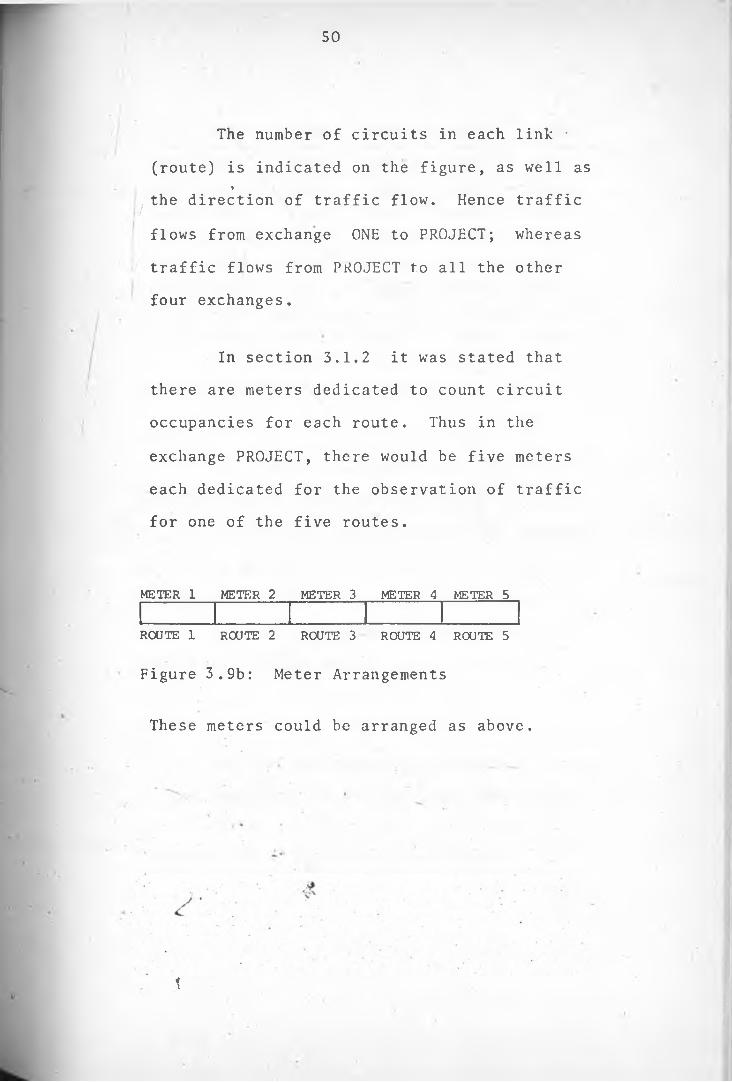
The number of circuits in each link •(route) is indicated on the figure, as well as
«the direction of traffic flow. Hence traffic/flows from exchange ONE to PROJECT; whereas traffic flows from PROJECT to all the other four exchanges.
In section 3.1.2 it was stated that there are meters dedicated to count circuit occupancies for each route. Thus in the
exchange PROJECT, there would be five meters each dedicated for the observation of traffic for one of the five routes.
METER 1 METER 2 METER 3 METER 4 METER 5 ... ■ - ' ------------------ ---------
ROUTE 1 ROUTE 2 ROUTE 3 ROUTE 4 ROUTE 5
Figure 3.9b: Meter Arrangements
These meters could be arranged as above.
1

51
METER 1 METER 2 METER 3 METER 4 METER 5
DAY 5 05000 30473 19860 04550 25200DAY 4 04050 30380 19600 04522 25100DAY 3 03190 30284 19250 04500 24900DAY 2 02240 30190 18930 04480 24000DAY 1 01390 30100 18600 04450 23900INITIAL 00450 30011 18342 04425 23845
ROUTE 1 ROUTE 2 ROUTE 3 ROUTE 4 ROUTE 5
Fig. 3.9c Example of filled table
Step 1The initial readings of the meters are
recorded before the beginning of the busy hour on the first day of measurements. The traffic measuring equipment (see 3.1.3) is started at the beginning of the busy hour and stopped at the end of the busy hour. The meter readings are again recorded on the row written DAY 1.
Step 2 .
The traffic measuring equipment is started at the beginning of the busy hour and stopped at the end of the hour. The meter readings are recorded on the ^appropriate row (DAY 2).
1

52N
This is repeated for five consecutive working days so that an average can be obtained to eliminate extreme erroneous readings.
Fig. 3.9c illustrates a completely filled out table with all meter readings for 5 days entered. For exchanges where no measuring equipment is available the busy circuits are simply counted and recorded) .
iStep 5.
By subtracting the initial meter readings from those taken on the first day the simultaneous meter operations for the first day are determined.
Similarly the circuit occupancy counts for the second day are obtained by subtracting the readings of DAY 1 from those of DAY 2. The same is done for days 3,4 and 5. Refering to equation 3.6; at this point in the measurement exercise the value of C has been determined for each route for each of the five days.
For our ^xample these values are shownj . ''inc Fig . 3.9d .
1

DAY 5 950 93 260 28 100DAY 4 860 96 350 22 200DAY 3 950 94 . 320 20 900DAY 2 850 90 330 30 100DAY 1 940 89 258 25 145
ROUTE 1 ROUTE 2 ROUTE 3 ROUTE 4 ROUTE 5
Fig. 3.9d Values of 'C’ (simultaneous meter operations)
Step 4 •
* Recall that for 60 minutes
• A - -Ac - 20 Erlangs 3.6a
Thus by dividing the values in 3. 9d by
20 the carried traffic in each route is obtained
in Erlangs. Fig. 3.9e gives the carried traffic
in the various routes iof our example.
Figure 3.9e.: Carried TrafficDAY 5 47.5 4.7 13.0 1.4 5.0DAY 4 43.0 4.8 17.5 1.1 10.0 ^DAY 3 47.5 4.5 16.0 1.0 45.0*DAY 2 42.5 4.5 16.5 1.5 ' 5.0DAY 1 47.0 4.7 .• 12.9 1.8 7.3AVERAGE
/45.5 •4*. 7> 15.2 1.4 6.9
* - Tills entry is disregarded as it obviously representsabnormal operation of some equipment.

I
54
i. The above procedure was followed for allswitching centres in the network in cooperation! /
with the personnel charged with the responsibility of maintaining the exchanges. Each person availed the traffic data observed through existing established procedures within the Kenya Posts and Telecommunications Corp which involved mailing the data to a central point from where it was collectively available. The measurements were done over the weeks of October to December of 1983 and the averages taken in each case.3.2.2 Results
The results of the measurements are presented in the tables of Fig. 3.10, where the average carried traffic intensity between automatic exchanges during the busy hour is given. The representation is in matrix form, with the originating (calling) exchanges listed on the left hand side of the matrix and the terminating (called) exchanges arranged as the columns of the matrix. This
. V % iarrangement gives an nxn matrix for a network with n switching systems. The entries in the matrix are each mdde up of two figures. The first figure gives the number of circuits making up the route, whereas the second figure gives the carried traffic in erlangs

55
As an example consider the matrix of Figure 3:10(b) with five exchanges, giving a 5x5 matrix..The interpretation is as follows. The route from Nairobi (NSC) to Kisumu is made up of 65 circuits and they carried 37.5 erlangs. Similarly for example the own-exchange traffic in Kericho is 12.9 erlangs,
but 48 circuits can be used to carry this traffic.
The entries marked HU are those routes usedI • ,as High Usage routes. This type of route is a first priority route for traffic and any excess traffic offered to this route overflows to an alternative route. This type of route can never be said to
have congestion. *
*
1

Fig 3 :10 ( a ) COAST NETWORK
EXCHANGE NAIROBI(NSC) MOMBASA(GSC) MALINDI BAMBURI D. BEACH CHANGAMWE MAKUPA .. NYALI
NAIROBI (NSC) 140/79.3 11/4.8MOMBASA(GSC) 150/101.6 126/82.2 * 29/7.0 24/22.1 17/8.9 55/47.7 74/39.2 54/30.2MALINDI 18/3.8 29/7.4 54/12.1 /BAMBURI 20/17.5 25/2.7D. BEACH 18/9.5 6/2.1CHANGAMWE 55/28.6 30/6.1MAKUPA . 70/27.9 25/2.0NYALI < 73/38.8
. .18/^7
KEY
x/y Route Consists of X circuits carrying y Erlangs.

F ig , 3 : 10(b) - KISUMU NETWORK
EXCHANGE NAIROBI(NSC) KISUMU(ASC) KISUMU(GSC) KAKAMEGA KERICHO NAKURU(ASC) NAKURU(GSC)
NAIROBI(NSC) 65/37.5 30/28.3HU 7/2.6 HU 56/21.6 32/28.0KISUMU(ASC) 66/31.5 48/30.9 16/9.4 17/12.3 14/2.0
7 8/5.1HUKISUMU(GSC) 30/26.3 48/32.2 132/30.9 5/3.6KAKAMEGA 5/2.2 15/11.0 5/2.1HU .36/10.5 \KERICHO 12/9.8HU 11/7.0 48/12.9 4/2.8™NAKURU ASC 54/35.2 14/4.6 54/16.6NAKURU GSC 32/28.5 8/4.8 4/2.4 54/35.5 108/40.7
V,
KEY <HU = High Usage Route x/y - Route consists of X circuits
carrying y erlangs.

F ig . 3 :10 (c) NYERI NETWORK
EXCHANGE NAIROBI(NSC) NYERI(ASC) NYERI(GSC) EMBU GSC MERU(GSC) KARATINA . NANYUKI
NAIROBI(GSC) 10/3.6 55/18.5HlJ 10/8.5HU 26/7.6HU 13/9.8HUNYERI(ASC) 22/9.1 45/3.8 10/6.3 18/3.7 5/1.4 •NYERI(GSC) 68/34.0 45/3.6 68/35.3 4/2.3 23/7 .9 4/2.1EMBU(GSC) 12/8.4 10/8.7 5/2.3 36/11.3 •
MERU(GSC) 29/9.9 19/7.9 54/18.3KARATINA 24/9.8 30/4.4NANYUKI 18/12.6 6/1.3 4/2.7 18/16.4 1
*<
KEY
HU = High Usage Route
Route consists of X circuits carrying y erlangs.
x/y

\
CTiLO
Fig. 3.10(d) - NAKURU NETWORK
EXCHANGE NAIROBI(NSC) NAKURU(ASC) NAKURU(GSC) ELDORETNAIROBI(NSC) 56/21.6 32/28.0HU 18/11.7HUNAKURU(ASC) 54/35.2HU ' 54/16.6 29/14.3NAKURU(GSC) 32/28.5 54/35.5 108/40.7- 7/4.4 ■ELDORET 31/24.2HU 29/13.3 7/4.7 46/10.0
KEY
HU = •High ;Usage Route* ix/y = Route consists of x circuits
> carrying y erlangs.

figure 3.loe: Nairobi netwc
EXCHANGE NAIROBINSC
NAIROBICENT.
NAIROBILTDM EMBAKASI EASTLEIGH KAR
NAIROBI NSC - 100/79.0 61/34.0 17/2.2 - 14/'
NAIROBI CENT. 100/95.2 427/24.15 133/69.2 17/14.6 - 40/
NAIROBI LTDM - 100/65.2 - 43/17.9 17/10.9 69/
EMBAKASI 18/3.7 19/1.0 33/11.7 18/2.7EASTLEIGH 15/3.2 20/17.9 10/2.6
KARIOBANGI 14/5.3 21/19.3HU 49/39.0 30/
PARKLANDS 19/10.6 20/18.7^ 70/49.9MILIMANI 40/17.5 e-,.- CHU 50/43.5 70/30.4 10/NAIROBI WEST 26/3.0 18/6.2 51/16.0
JAMHURI PARK 20/9.7 34/23.8HU 45/32.5
NAIROBI SOUTH 27/16.8 32/28.0HU 45/21.5LANGATA 10/6.0 32/23.3UTHIRU 3/0.5 9/1.8 16/8.9KIKUYU 15/9.1
KABETE 10/1.9 28/22.9
GIGIRI 10/1.7 , HU 10/5.2 29/14.8

61
CHAPTER FOURGRADE OP SERVICE ON TELECOMMUNICATIONS LINKS
So far traffic data giving the traffic flowing in various links in the busy hour has been obtained. This data will next be used to assess the network as it exists and evaluate to what extent it meets its objectives. One of these objecti ves is to provide an acceptable grade of service to the users on the network.
The grade of service can be expressed as a blocking probability or a percentage of calls permitted to fail.
In Chapter 3 call congestion was defined as
B = Blocked Calls Offered Calls
A - A_ o c 3.5a
Now another parameter, time congestion E is defined as
E =- . , Time during which all circuits are occupied
Duration of measurements.*
^ In full civailabi 1 ity systems where calls arrive at random B - E. With limited availability and/or other call arrival distributions E / B, the difference
being small enough to be ignored in some cases.

62
A number of factors are considered whendeciding on the numerical values for the grades of1/ .service at various points in a telecommunicationsnetwork. Some of these factors are customer require
.ments and expectations, equipment costs, loss of revenue due to blocked traffic, unforseen traffic loads and safety margins necessary to cover errors in traffic estimates. The actual grades of service chosen represent a compromise of all these require' ments.
In practice the grade of service offered to users may be worse than that which was designed due to technical faults, dimensioning errors or unimple mented installation projects among other reasons.
In Kenya the designed grades of service between switching systems are given in the Figure 4
below.
From To - - GOS(Exchange) (Exchange)Automatic Automatic • 0.01Automatic Manual 0.03Mapual v* Automatic • 0.1Ownrexchange 0.02
Fig. V l Designed Grades of Service (Obtained fyorn the KP & TC traffic Department)•

63
It is observed from the table that the best grade of service is expected between two automatic exchanges; whereas-maximum blocking is expected between two manually operated switching systems.
In this chapter- we seek to investigate whetherthe designed grades of service are met on the routeslinking automatic exchanges. Automatic measurementsof call congestion B would require two accumulatingcounters, one counter incrementing whenever a callenters a system and the other incrementing for each
blocked call. The measurement of time congestion Erequires a counter so connected to accumulate thetime periods during which all circuits are occupied.In the systems considered the measurement facilitiesfor the quantities E and B are not incorporated, andit was therefore necessary to estimate the congestionencountered on each group of circuits from the traffic
... | - .... *
intensity measurements of Chapter 3 . This was doneusing a simple computer programme developed for this purpose.
4.1 Traffic Theory Models
,'In order to 'estimate the blocking encountered on the various links the relevant model to describethe behaviour of telecommunications traffic must be
1 . determined. Some of the standard telecommunications

6 4
traffic theory models are the pure chance traffic model, Erlang loss model and the Engset distribution model. Each of these models involves certain
assumptions as summarized below^.
4.1.1 Pure chance traffic■ ■ ■ — — — ■ - —•
This model makes the assumptions that:-. . \ ’ i
a) there is an unlimited number of circuits available so that no call that arrives is
rejected.b) calls arrive at random with a mean arrival
rate.cj the calls holding times are exponentially
distributed.
This is an idealized model and forms the basis for other model theories.
4.1.2 Erlang Loss Model
The assumptions made with this model are:-
a) calls arrive at random and rejected calls*• /
(due to all circuits being busy) do not *j V'
^ return.b) The probability of a call arriving at the
system is independent of the state of thesystem.
65
c) the system is in statistical equilibrium.d) The number of sources that generate calls is
infinite.e) there is full availability of the circuits in
the system.f) the holding times are exponentially
distributed.
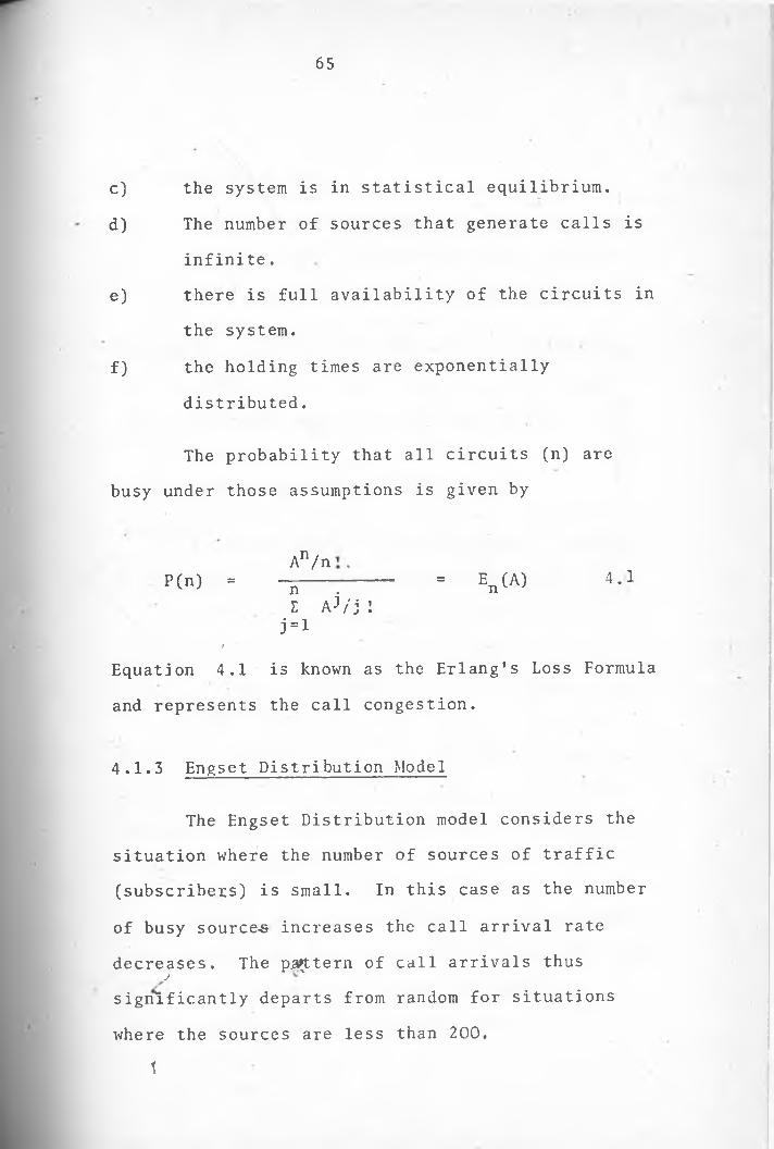
The probability that all circuits (n) are busy under those assumptions is given by
An/ n .p(n) = -j--- :----- = En (A) 4.1
e AJ/j :j=l
t
Equation 4.1 is known as the Erlang’s Loss Formula and represents the call congestion.
4.1.3 Engset Distribution Model
The Engset Distribution model considers the situation where the number of sources of traffic (subscribers) is small. In this case as the number
of busy sources increases the call arrival ratedecreases. The pattern of call arrivals thus
j
significantly departs from random for situations where the sources are less than 2 0 0.
\

66
The assumptions are:
a) holding times are exponentially distributed.b) there is full availability of circuits and
all lost calls do not get repeated.
The Engset distribution model would be useful in the determination of time congestion for routes linking manually operated switching systems.
4.2 Computer Programme "ERLANG B" -
In this section a simple computer programme is developed to evaluate the offered traffic (A ) to a group of circuits of a known size (N) and over which a known (measured) traffic intensity (Ac) flows. In the development of the programme it has been assumed that pure chance traffic is offered to a full availability group of circuits and that all lost calls are cleared. It is thus assumed that when a caller encounters congestion he does not make a repeated attempt.
Whereas this assumption may not seem realistic other models have £een proposed^ which show that
j sthe effect of repeated attempts is simply to increase the average call arrival rate.
4

67
The Erlang loss Model is thus assumed.
The basic equations used to estimate theioffered traffic are:-
Ac = A0/UrB) 4.2
BA > !nE=o a J/J '
4.3
where offered traffic (Erlangs) carried traffic (Erlangs) number of circuits
congestion.
Equation 4.2 relates the offered traffic to a group of circuits to the traffic carried by the route and the congestion encountered by this traffic Equation 4.3 is the congestion function which relates the offered traffic and the number of circuits comprising a route, to congestion under the assumptions above (Erlang Loss Model)
The procedure adopted here is to initially*assume^that all the' offered traffic is successfully
carried. The measured value for carried.traffic Acis thus substituted for the offered traffic An in
1 . equation 4.3.

This gives
B
68
An/n!cnZ
4.3a
j=laJ/j:
The value of congestion B-. is then inserted »into equation 4.2 to obtain
Aox - 4.2a
A is the traffic offered when A„ erlangs is°i . . .carried in a route of n circuits with congestion
Bjj and is the required estimate for the offered
traffic.
The value |A -A ! reveals whether or not a ' o^ csignificant amount of congestion was encountered
on the route.
Figure 4.2 illustrates a flowchart of the programme. It consists of one main programme - (Fig. 4.2) and
a subroutine .(Fig. 4.2a). The subroutine calculates factorials, utilizing one loop.
The main programme calculates congestion usin^equation 4.3ta) with the carried traffic (Ac) and the number of circuits (n) as the known variables.
1

69

70
The value B- thus obtained is then used to evaluate the offered traffic AQ from equation 4.2(a) the carried traffic (Ac) and the number of circuits (n).
Figure 4.3 is a printout of the programme illustrated in the flow chart. This programme has been written in the FORTRAN language and was developed on the WANG PC microcomputer. The figures for carried traffic (A ) , offered traffic (Aq), congestion and the number of circuits (n) have
been defined as real. It is however necessary to represent figures obtained from the summation and factorial functions in their double precision forms as they are beyond the range .of the microcomputer.
4.3 Results
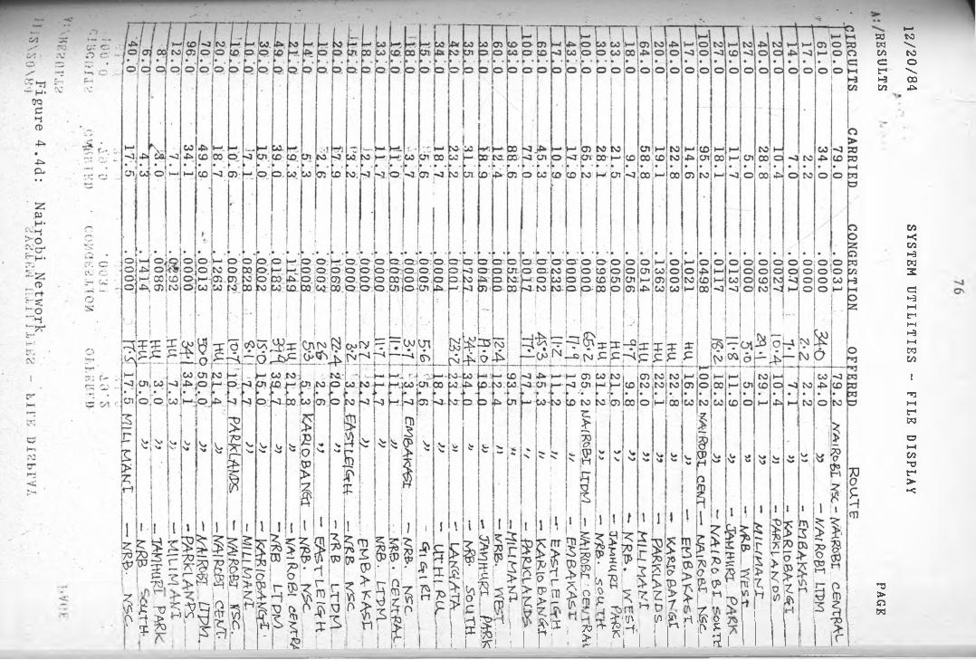
The programme Erlang B was run using the data in Chapter 3 for the various routes linking automatic (crossbar) exchanges. The results are provided by way of a printout of the output file
• x1* ' .’RESULTS’ and are presented in Figure 4.4.
The printout* consists of four columns headedX 7 .’circuits’ (number of circuits in the route),’carried’ (carried traffic in erlangs), ’congestion’ (estimated grade of service offered on the route)
and ’offered’ (estimated offered traffic in erlangs).

Figure 4.2a: Flowchart for SubroutineLGFACT

72
C PROGRAM ERLANG BINTEGER YREAL AOFF,CONG, N, C
•' DOUBLE PRECISION SUM,U,JFACT,Z,Q,X,J OPEN(8 ,FILE= * RESULTS’,STATUS=’NEW’)WRITE(8,25)
25 FORMAT(2 X, ’CIRCUITS’,4X, ’CARRIED’,4X, ’CONGESTION I WRITE(*,5)5 FORMAT(2X,’INPUT TWO NUMBERS XXX.X AND XXX.X AND
READ(*,15)N,C,Y 15 FORMAT(F5.1,F5.1,13)
IF (Y.EQ.999)GOTO 100 X = N Q=C J= IDO SUM = Q
10 J-Jh-1CALL LGFACT(J,JFACT)U-Q**J/JFACT
j - SUM=SUM+U Z=Q**JIF(X-J)10,20,10
20 CONG=U/SUMAOFF=Q/(1-CONG)• WRITE(8,30)N,C,CONG,AOFF
30 FORMAT(3X,F5.1.7X.F5.1,8X,F5.4,8X,F5.1)GOTO 1
100 CLOSE(8 )STOPENDSUBROUTINE LGFACT(J,JFACT)DOUBLE PRECISION JFACT,J,KK = J-1JFACT=J*K
35 IF(K-1)40,45,4040 K=K-1
JFACT=JFACT*K GOTO 35
45 • RETURNEND
Figure 4.3: Programme to evaluate offered traffic .
given carried traffic A , and number of -! circuits n.
v''
, 4 X, ’OFFERED INTEGER XXX’
1

73
01/01/84A;/RESULTS
SYSTEM UTILITIES - FILE DISPLAYPAGE
70.025.073.018.0
CIRCUITS CARRIED CONGESTION OFFERED14 0 .-Q____ ____ 79.3 ____ .QQOOl 71*3 i 7 9 .3 MA [Ro0>C WSC - M6MBAS/V GrSC
11.0 _ 4 . 8 _____.9095 . . . . t 4^8 >) - XA4L IN/'Dri50..t_0__. ____ 1QJL^6_ ___ . oqoo: IO(-&i01.6 ASA ^<c12 6 .0 1 82 .2 .0000 r — ' 8 2 . 2 » — yioMBAsA ’
2 9 . 0 ... . 7 . 0 .0000 l O j 7 . 0 >) , - A4AL/ n/DI__2.4 ._Q _ 2 2 J L _ .J.064' 2f-0 24 .7 » - BA M BU £ I
17.0 ____ 8 . 9 _ _ ,_.QQ53; 8'9 8 j 9 - P /A .V I BFAclV. . 6 0 . 0 ... -_-.47..JZ_____ .0363| 50-7 49 .5 »• — CH- A t-vc% AfA
74.0 „ _ 39 . 2_____ . QQQQ1 . ^ • 2 - 39 .2 V ^M AiCLtPA_54.0 .30.2__ ___ .0000 30-7.30.2 n > • - N / V A U
18.0 3 . 8 .oooo; 3^1 3 . 8 M A L l h f & r — A/RB_2 9 . 0____ 7.4 . o o o o! 7'4 7 . 4 — WSA- Sr^r-
54.0 12.1 .0000! IL'U 12.1 - A^AUKJPr20.0 17.5 .0973 Z 4 19.4 PrtM&URi: . — . KsA ctSC.25.0 2 . 7 .0000 2*1 2. 7 - £>A H B l lR l18.0 9 . 5 .0047 9-S 9 . 5 Pi AWE »B 4ctt ^ s< z . —
' 6 . 0 2. 7 .0396 ZS 2 . 8 J; - P 7 A N t BFA55.0 28 .6 .0000 i K lo
jCO >• CD s > f > £ £ - MSA < ^sc
' 3 0 . 0 6.1 .0000 . fell 6 . 1 -C hiA U G tA V l'C &212
38. 0 000
0000 2fO 2.0 _ZX_8 0000
4.7 ,_2£-6 38.8 L-r 4.7 _ __ — \jA& c LX___
Figure 4.4a: Coast. Network

74
12
A •
/20/84
/RESULTS
CIRCUITS
SYSTEM UTILITIES - FILE
CARRIED CONGESTION OFFERED
DISPLAY
Route
0
PAGE
----567U 21.6 .0000 Z1-& ‘21.6 fv'AiPo'&r KSc - A/AKUL-RUL AtS c.32.0 28.0 .0665 3Z•'b |3 0.0 - MKUR.U,
— T O 11.7 . 0225 l2-ojL2_0^ - elpd k e r54.0 35.2 .0007____ 35*213 5.2 A/AKURM. A$c — NP-G fVSc-54.0 16.6 .0000 16.6 - IVAKURO. <SrSC-
* 29.0 14.3 .0002 143 14.3 - elpcrbt32.0 28.5 .0736 C.32'0 30.8 f AUuRJX <=r£c — /vai Rc>E»r r /st-54.0 35.5 .0009 35.5 —\K/AKURjJ_ __
-----7.0 4.4 .0855 AH 4.8 - EL-^REr—31.0 24.2 .0321' Z&5125.0 ELJDdR»£T — NAlRo&T isr .Cj 29.0 13.3 .0001 _S3iA.13.3-----770 4.7 . 1031 S*£ 5.2 — A/AkuRU ^-^670 10.0 .0000 \o*o10.0 — E=L£>6 fR.&*r
/
Figure 4.4b:Nakuru Network!
/C.
*V'
1

75
a./RESULTS PAGE
■l2/20/84 SYSTEM UTILITIES - FILE DISPLAY OG
CIRCUITS C ARRIED______CONGESTION-___ OF FERED__________-----6 5 . 0 3 7 . 5 . 0000 m 3 7 . 5 VAlRoBr bf<u k i s u m
-Kisu vwl . <ks c.3 0 . 0 2 8 . 3 . 1031 n a 3 1 . 6 _ J)7 . 0 2 . 6 . 0 1 2 9 H a 2 . 6 33
' 6 6 . 0 3 1 . 5 .0 0 0 0 Si-£ 3 1 . 5 K ISU MLL___ASc__rcs-ATUEPBi M S c~ T 8 . 0 3 0 . 9 .0 0 1 0 % >'3 3 0 . 9 » ~K_ISuMU 4 s c ,
1 6 .0 9 . 4 . 0 1 4 9 9 . 5 5V - KAKA" 1 7 . 6 1 2 .3 .0 4 6 7 lA 'Z 1 2 . 9 3v _ K E R IC H *~ 1 4 . 0 2 . 0 .0 0 0 0 Z'O 2 . 0 3) - HASOjUQUL a SC..
— 30.0" 2 6 . 3 .0 7 1 1 3o*0 2 8 . 3 u:laumu. Q r ^
1 . o - 3 2 . 2 ~ " .0026 3 2 . 3 io^ u h u . a s c5 . 0 3 . 6 . 1686 5* l_ 4 . 3 33 - k^HKAMe^-A ~7O ) 5 . 1 .0 7 5 3 . HU,. 5 . 5 335 7 F 2 . 2 .0 5 5 1 2 . 3 KAKAHterA".„ 7~ a/a i Zp B>i _t/S e.
- T 5 . 0 1 1 . 0 ““ . 0 5 8 8 2sJJ 1 1 . 7 ' 3 J A s c .‘ 5 . 0 2 . 1 .0 4 8 6 n a 2 . 2 JJ -^iSUMU.“ 3 6 . 0 1 0 .5 .0 0 0 0 1 0 . 5 yy _ K A K A ^ e c r A . ..— T2T0 9 . 8 .1 1 2 1 Ha 1 1 . 0 WPI?lCHr. -K/AlRPei NSc-
1T70 7 . 0 . 0 4 7 8 7 . 4 V *" KJ5 UKA.U A s e■"'4870 1 2 . 9 . 0000 iz*9 1 2 . 9 jy ~ k: e E.i^.hc» _ ----------
4 / 0 ---------2 . 8 ---------- . 1 9 7 9 n a 3 . 5 yj — N/AKURU. a“ X 4 : o . . ... 4 . 6 .0 0 0 2 4'& 4 . 6 VAkUlfeiL A s c , - KiSUMU A^C-
5 4 . 0 1 6 . 6 .0 0 0 0-----l-V —
!£>•& 1 6 . 6 by - A//\KURU8 . 0 4 . 8 . 0615 4 3 5 . 1 IsfAlCURU £tS<\ — KlSUMU. ..4 . 0 2 . 4 .1 5 4 2 27 2 . 8 - KEfi.1 C-tto
5 4 . 0 3 5 . 5 . 0 0 0 9 3 * ? 3 5 . 5 j>y - / ^ K U R U A Sc: j_ 1 . 0 .0 .. .. 3 . 0 . 0 0 0 9 3-0 3 . 0 A/AI &£>Pfr m s c — A $ c
5 5 .0 1 8 .5 . 0000 n a 1 8 . 5 : - N Yfc& r <3rs c.10 .0 • 8 . 5 . 1446 nU 9 . 9 f/ .. ^ MB lA- - -2 6 .0 7 . 6 . 0000 HU . 7 . 6 n - . .13 .0 9 . 8 . 0 7 7 9 HU 1 0 . 6 b . - fv/AN'YUlC.r .
_ 2 2 . 0 . 9 . 1 . 0 0 0 1 9 . 1 kVE RX ASCL - h/A!RC>e>r__NSc.4 5 .0 3 . 8 .0 0 0 0 3 . 8 _)?10 .0 • 6 . 3 . 0 5 2 9 .... && 6 .7 X - £ vAB a18 .0 3 . 7 .0 0 0 0 3'7 3 . 7 35 -
5 . 0 1 .4 .0 1 4 7 A 'A l 1 . 4 43 — N A f / x U ICl _
'F igure 4 .4c : Kiisumu Network' Ny er i Network
3TH i 5 * , « ? " * ! ! Si n
§f w f c g *bin r pn ir*KJn i r s f
wMC/ict-1*-3co
*0>ow
12/20/84 SYSTEM UTILITIES - FILE DISPLAY

20/84
SYSTEM U
TILITIES -
FILE
DISPLAY

78
In order to evaluate the extent to which the designed grade of service is met on the routes thej •I / \various networks are considered case by case.
4.3.1 Coast Network
• In the coast network the offered grade of service in the majority of routes is equal or better than the designed value. The three routes which result in unacceptable blocking of traffic are:
Route from Mombasa to Bamburi with congestionof i nRoute from Mombasa to Changamwe with Congestion of 4$The own-exchange route for Diani Beach with congestion of \%.
4.3.2 Nakuru Network
In the Nakuru network approximately 50°o of the routes do not meet the designed grade of service Significant congestion is encountered on four routes namely:
Routej
&f 7%
from NairobiV' to Nakuru with congestion
Route from Nakuru to Nairobi with congestion 9 f 7%
y

79
Route from Nakuru to Eldoret with congestiQn of 9«oRoute from Eldoret to Nakuru with congesti0n
iof 1 0$
»Other congested routes are:
Route from Nairobi to Eldoret with congest^on of 2$Route from Eldoret to Nairobi with congestion of 3$
4.3.3 Kisumu Network
Eight routes out of the total twenty five routes have congestion in excess of the designed, grade of service of 0 .0 1.
These routes are:-
Route from Kisumu to Kericho with congestion of 5$Route from Kisumu to Nairobi with congestionof 7$* \ »Route from Kisumu to Kakamega with congesti0n of 17$
£ Route from Kakamega to Nairobi with congesti0n of 6 $Route- from Kakamega to Kisumu with congestion of 6 $

80
Route from Kericho to Kisumu with congestion of S%
Route from Nakuru to Kisumu with congestion of 6 %
Route from Nakuru to Kericho with congestion of 15 %
4.3.4 Nyeri Network
Of the ten routes in the Nyeri network only one route from Nyeri to Embu is found to be congested
4.3.5 Nairobi network
This is a network comprising 17 switching systems and has a large number of High Usage routes.A few of the routes in this network were found to have unacceptable congestion levels
Route from Nairobi Central to Nairobi NSC with 5% congestionRoute from Nairobi Ltdm to Eastleigh with S%
congestion
• Route from Nairobi Ltdm to Milimani with congestion ^
route from Nairobi Ltdm to Nairobi South with 7% congestion.
Route from Eastleigh to Nairobi NSC with 101 congestion
81
Route from Kariobangi to Nairobi Ltdm with 2 % congestion.
/Route from Kariobangi to Milimani with 8%
congestionRoute from Langata to Nairobi NSC with 4% congestionRoute from Langata to Nairobi Ltdm with 2%
congestionRoute from Uthiru to Nairobi NSC with 10% congestionRoute from Kikuyu to Nairobi Ltdm with 2%
congestionRoute from Kabete to Nairobi Ltdm with 5% congestion
4.4 High Usage Routes
High Usage routes where no congestion is recordable since excess traffic overflows into a lower priority route have been indicated. The entries in the column 'congestion' for these routes indicate the blocking that would exist if the routes were not high usage.
*: j . * . . .c. ■ ■
1

82
4.5 Comparison of Conventional Methods of obtaining Aq with the 'Erlang B' Programme.
i/.
The normal practice within the Kenya Post,
and Telecommunication Corporation is to estimater .offered traffic on a given route by use of tables.In particular the tables from "TELEVERKETS CENTRALFORVALTNING, Stokholm are used. The tables can be used for traffic ranging between 0 . 1 - 80.0 erlangs and for routes containing between 1-105 circuits.
The values of offered traffic calculated by use of these tables are shown on the 4th column, and shows very close correspondence to those values resulting from the Programme 'Erlang B1. The biggest difference in the two values is for the route for traffic flowing from Bamburi to Mombasa GSC, where AQ obtained from calculations using tables is 19.4 erlangs; and Aq obtained by the Programme is 22.4 erlangs. This represents a difference of 3 erlangs.
Conclusions from the Results— :------- 7 --------------— ------- --------------------------c .
The programme 'ERLANG B' developed in thischapter gives a good estimate for the offered• . 1
traffic given the number of circuits and the carried
traffic measured on the route.
83
The effectiveness of the programme is deduced by observing that the largest deviation of AQ from that obtained using traffic tables is approximately 3 erlangs. All other deviations are much smaller than the 3 erlangs observed in the worst case.
i
Because of the assumptions made to obtain in equation 4.3a, B- may not always represent
the exact congestion encountered. However, it can be stated that in all cases the congestion is greater than or equal to B1
• that is congestion B-
The programme ’ERLANG B’ is thus a sufficient tool that can be used to assess the status of a network consisting of relatively large automatic switches linked by circuit groups, each of known sizes carrying known traffic. By status it is meant that each link can be categorized as congested
or not congested. The traffic that is blocked as a result of t'his congestion can be estimated. On heavily congested routes however the resultingestimates of offered" traffic are used with caution■* cbearing in mind that a possible deviation of upto3 erlangs could exist.
1

84
From the results of section 4.3 it is also concluded that a fair percentage of the links in the telecommunications network are congested to proportions which would be unacceptable as compared to the design values. The service offered on these routes is of lower grade and causes significant
blocking of telecommunications traffic. The percentage of the congested to non-congested routes varies from network to network as follows:
Coast network 13%Nakuru network 50%Kisumu network 32%
Nyeri network 1 0%Nairobi network 14%
Overall an approximate 24% of all the linksconnecting automatic exchanges are considered to be offering a grade of service below that designed.
1

85
CHAPTER FIVE*--------------- /
DEMAND FORECASTS —j /i
In an ideal telecommunications network where no 'restrictions exist, traffic forecasting and planning would ensure that demands for telecommunication service are accurately foreseen and satisfied as they arise.In a developing country like Kenya however, the time lag between identification of need for service and the ability to meet this need is considerable. In some cases the time lag has been known to exceed 10 years
as a result of economic constraints. This means that accurate forecasts are of utmost importance if the necessary plant is to be available before existing capacity is exhausted. Further to this errors in forecasting can prove very costly for a telecommunications organisation. For example over estimation results in unnecessary investment in expensive equipment which earns no revenue. Underestimation on the other hand results in losses of
revenue that could be earned and renders the network inadequate.
*/ . . . .Jk further drawback in a developing network is
the fact that existing requirement for service is often ndt satisfied. This gives rise to a situation

86
where at any one time there are demands on the network that cannot be served. By only considering existing users of the network for forecasting purposes these demands are hidden causing innaccurate forecasts.
iIt therefore becomes necessary to assess the network to determine to what extent the requirements on it are met before forecasting for future growth.
5.1 ASSESSMENT OF THE NETWORK FOR UNSATISFIED DEMAND
The demand and growth characteristics of telecommunication service varies from region to region and is dictated to a certain extent by various exogeneous factors such as population growth and distribution, income, industrialisation of the area,
stage in development and the general occupation of the community among others. A general assessment of the whole network would thus give misleading results.
In this section the five major towns (Nairobi, Mombasa, Kisumu,~*Nakuru, Nyeri) have been consideredseparately to determine the manner in which demand
j
for service has been satisfied. Reference to Figure 2.6 shown that these are Area Switching
Centrel (A.S.C.) regions and due to the
87
heirarchical nature of the Kenyan network their »i
growth and demand characteristics would be representative of the characteristics of the Group Switching Centres (G.S.C.) and End Offices (E.O.) connected to them.
5.1.1. Data Presentation
For each of the stations the necessary data was obtained and recorded in a table, as illustrated in the tables of Figure 5.1.
The first column gives the year under
consideration. In the second column the number of connected users is entered. This represents the number of actual telephone pairs in use and no categorisations are given. The third column has the number of waiting users in the area and represents the unsatisfied demand. The fourth column is a total of the second and third column and is considered as the’total demand* for service in the region. This
\ w represents the number of would be users in an ideal
situation where unlimited plant is available andtelecommunication Service is provided on request.The final column indicates what percentage of thetotal demand is contributed by the waiting users.
1

8 8
KISUMU
Year(a)
Connected Users (b)
Waiting Users (c)
Total Demand (b+c) e ‘ f %
1965 729 53 782 6
1966 755 84 839 10
1967 735 152 887 171968 860 158 998 141969 1051 162 1113 151970 1107 165 1272 131971 1276 382 1658 231972 1384 593 1977 301973 1711 258 1969 15
1974 1829 447 2276 20
1975 1904 651 2555 251976 2162 568 2730 21
1977 2253 431 2884 161978 2292 586 3127 v 191979 2490 650 3140 21
1980 2868 621 3489 181981 3205 ” 706 3911 181982 3424 1045 4469 321983
■4,3594
<L•*1163 4757 24
Avg. = 18%
Figure 5 .1a : Kisumu

89
MOMBASA
Year(a)1
Connected Users (b)
Waiting Users (c)
Total Demandd = b + C e = c % c 3 .
1965 4378 140 4518 31966 4532 318 4850 6
1967 4724 478 5202 91968 4951 649 5600 12
1969 5260 532 5797 91970 5382 1249 6631 191971 6125 1337 7462 181972 6917 1275 8192 161973 7026 1886 8915 21
1974 7252 2 360 9612 251975 7663 2545 10.008 251976 8408 3247 11,655 281977 . 9357 1921 11,278 171978 •• 9770 3045 12,815 241979 10,255 3897 14,152 281980 10,643 5035 15,678 321981 11,719 5474 17,193 321982 12,278 6822 19,100 361983 12,926 6505 19,431 33
/ . . . .C ’ Avg = 21%
Figure 5 . 1 b . : Mombasa
1

90
NAKURU
—
Year(a)
Connected Users (b)
Waiting Users (c)
Total Demand d = b+c e " | ° 6
1965 1137 10 1147 • 1
1966 1186 47 1233 4
1967 1238 74 1312 6
1968 1236 107 1343 8
1969 1217 136 1353 10
1970 1255 251 1506 17
1971 1561 266 1827 15
1972 ' 1756 282 2038 14
1973 1754 289 2043 14
1974 1822 490 2313 21
1975 1931 716 2547 27
1976 2353 365 2718 13
197 7 2658 255 2913 9
1978 2847 365 3212 11
1979 2897 583 3480 17
1980 2951 1031 3982 26
1981 3078 1739 4817 • 36
1982 3132 2014 5146 39
1983 3558 2880+
6438 457
Avg = 18°&
Figure 5 . 1 c : Nakuru1

91
NYERI
- •• ■ -Year(a)
Connected Users (b)
Waiting Users (c)
Total Demand d = b+c e ■ 3*
1965 862 152 1014 151966 870 198 1068 191967 932 178 1110 161968 1014 248 1262 20
1969 1043 219 1262 171970 1076 343 1419 241971 1262 402 1664 241972 1524 273 1797 151975 1683 308 . 1991 151974 2066 34 3 2409 . ]41975 2266 847 3113 271976 2517 1091 3608 301977 2937 1751 4688 371978 3034 1845 4879 381979 3398 1865 5263 351980 3916 2727 6643 411981. 4022 3598 7620 471982 4500 4691 9191 511983 5072 ~ 4992
■pv10,064 50
Avg = 281
Figure 5 . Id : Nyeri1

92
* NAIROBI (INDUSTRIAL AREA)
Year(a)
Connected Users (b)
Waiting Users (c)
Total Demand d = b+c
1965 1189 118 1307 91966 1255 448 1703 261967 1307 579 1886 311968 1425 510 1935 261969 1985 465 2450 191970 2388 519 2907 181971 2650 1134 3784 301972 3008 1720 4788 361973 4352 2115 6467 33
1974 4410 2019 6429 311975 4564 2441 * 6490 351976 4498 2030 6528 31197 7 4579 2004 ' 6583 301978 4758 2356 7114 331979 5028 4055 9083 451980 5142 4227 9363 451981 5303 5390 10,693 501982 5809 6292 1 2 ,1 0 1 52
1983 6309 6912 13,221 52
Avg - 33%
Figure 5 . 1 e : N a irob i I n d u s t r i a l Area1
CL|0 O'O
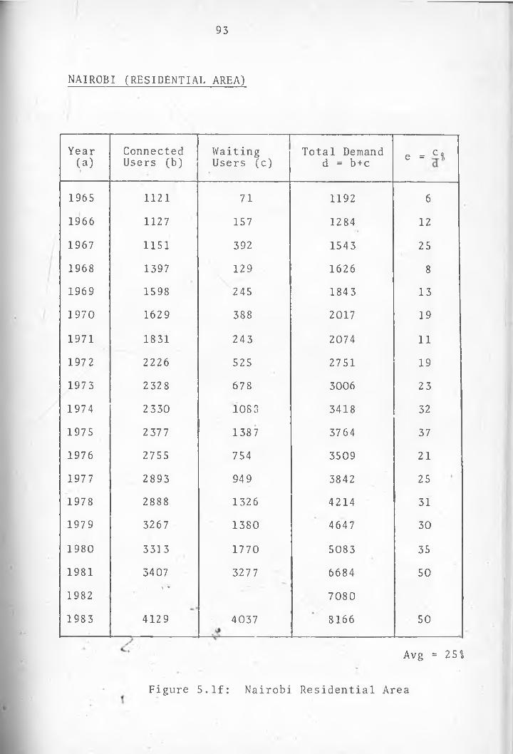
93
NAIROBI (RESIDENTIAL AREA)
Year(a)i
Connected Users (b)
---1Waiting Users (c)
Total Demand d = b + c e = c %e
1965 1121 71 1192 6
1966 1127 157 1284 12
1967 1151 392 1543 251968 1397 129 1626 8
1969 1598 245 1843 131970 1629 388 2017 191971 1831 243 2074 11
1972 2226 525 2751 191973 2 32 8 678 3006 231974 2330 108 3 3418 321975 2 37 7 1387 3764 371976 2755 754 3509 21
1977 2893 94 9 3842 251978 2888 1326 4214 311979 3267 1380 4647 301980 3313 1770 5083 351981 3407 3277 6684 501982
\ *7080
1983 4129 4037 8166 50
Avg = 2 5
Figure 5 . I f : N a irob i R e s i d e n t i a l Area
O'®
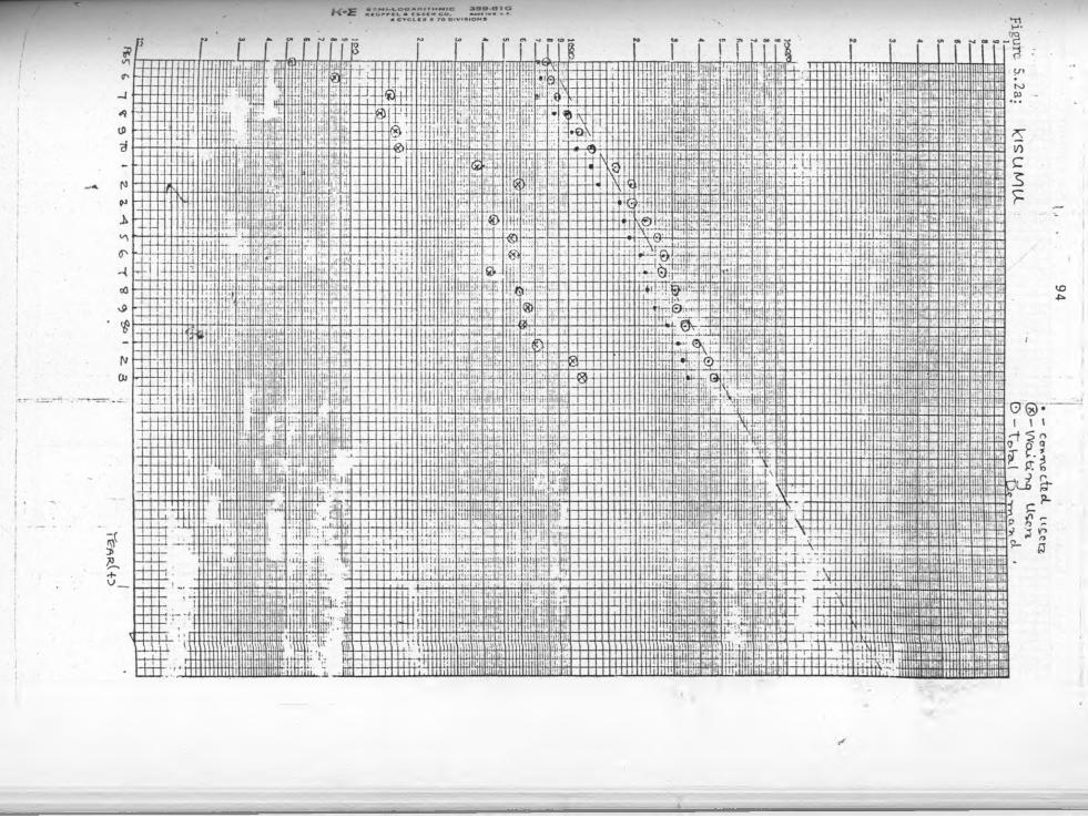

i « L *) S
CV)


*va
j,
F 1
I •<
« M
i.
"9
& V
*
2 b
L
*&>,
v**\«U
- o
I'd 3
VN

98

«**>!•
K*E’ r ; s c m i-i o o a r i t h m i c 3 5 9 -8 1 G ■ccurriL • e s s e * co. u m i m . i.l* C Y C L E S X 7 0 O I W I B I O M S
\S>VC

100
The data presented dates back 19 years and it was anticipated that meaningful conclusions could be drawn from it. This data has been plotted on semi-log paper and the plots are presented in the graphs of Figure 5.2.
5.1.2. Observations from the Data and Plots
From the data and graphs the following is obeserved:-
In all the areas considered the demand for telecommunication services has not been met. Infact in the 19 year period considered the number of waiting users tends to increase although in a rather random fashion. A look at the last column of all the tables shows that a significant percentage of the total demand consists of unserved waiters.In the worse cases as much as 50% of the demand represents waiters. In otherwords only half of the users requiring service can get this service under this situation. It is inferred from these observations that thejre is inadequate telecommunication plant ifc the network to cater for the demand.
♦One reason f o r t h i s inadequacy i s the la ck o f
101
revenue. However another reason could be that the demand as it exists was not foreseen, in other words there were no accurate forecasts to enable the right amount of plant to be availed. The fact that the unsatisfied demand tends to increase with time in all areas points to the fact that forecasts do not take this hidden demand into consideration.
A comparison of the 5 areas reveals that the situation is worst in Nairobi’s Industrial area where over the 19 year period an average of 33% of demand is attributed to waiting users. This would be expected as growth in such an area is bound to be more rapid than in a residential area, since a household need only have one telephone, but an industry’s requirement for telephones grows with the growth of the plant. Nakuru and Kisumu are perhaps better served with an average of 18% of demand being from waiters.
A look at the graphs of connected users vs time shows that the'growth ’flattens’ out when the'waiters' graph climbs Steeply. A good illustration
4 ^ • of this is the Nairobi Residential area case, betweensay 1972 - 1981. In this period of time the numberof users grew from 2226 to 3407 representing a growth

102
of 1181 whereas the number of waiting users grew from 525 to 3277, a growth of 2752. An explanation for this is that during this period the plant had been exhausted and no more users could be provided with service. But the requirement for service is not dependent on availability of plant and continued to be registered.
Similar behaviour can be seen in the other cases as well. Consider Nakuru in the period 1970 - 1982. We notice that in the period between 1972 - 1975 the connected users’ graph remains fairly flat whereas that of 'waiters ' experiences a steep climb. Between 1975 and 1977 a climb in the connections graph is accompanied by a fall in the waiters’ graph, and between 1977 to 1982 the waiters increase steadily while the number of connections remains fairly constant.
The above illustrates the fact that accumulation of waiting users is inversely dependent on the capability of the network to accommodate new users.
*VAJ
As previously mentioned the demand is considered to be the additive combination of the connected*users and the waiting users. A look at the

1 0 3
graphs of demand/time for Kisumu, Nakuru, Mombasa
and Nyeri reveals that the plots approximate to a straight line on semi-logarithmie paper. The plots for the Nairobi area reveal deviations from a straight line. The approximately straight line plots indicate that the demand grows in an exponential fashion4'.
5.1.3 Choice of Model for the growth of Demandfor Telecommunications Service
The simplest exponential model that could be used to describe the growth of the demand for telecommunications service would be of the form
al + a2te
where y = demandt = time in years.
The growth rate of any model as defined for one period of time is
.i yt + i ~ . yt + i - ?t(t + 1 - t)yt yt
5.2
where y = demand at time t

'
104
The limiting growth rate for a continous function is given by
R(t) lim y(t * at) - y(t) At-^0 At y(t)
5.3
Thus for the exponential model the growth rate would be
R(t) d (eal + a2^dt
ai + a2tal + a2t
al + a2t5.4
a2 = az = constant
This suggests that constant growth would be expected and'may not always be absolutely true. Another model that could be used and that takes care of the variabilityof the growth rates is the logistic growth function-
y(t)l'+ exp (a- + a2t)
5.5
where 1 k constant representing an upper
limit to growth.

105
A graph of a logistic growth curve is illustrated below in Figure 5.3.
Figure 5.3: Logistic Growth Curve
For smaller values of t the function shows exponential growth. As t increases y(t) approaches 'the saturation value y^.
A look at the set of graphs in Figure 5.4 reveals the fact that in all the areas, the growth is in the exponential portion of the logistic growth curve, (that is between and X?) and does not approach saturation. For this reason in theforecast period under consideration the growth of
j ^demand can be considered exponential, and the model
al + a2 tt 7 = eis adequate.

106
\

r
107/
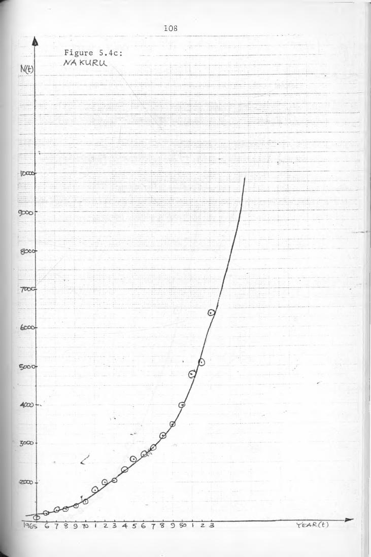
108

109

OO ‘av
aj,~tV
<4!pc9'I (iN/D
a^rP-i^L /VPeAj • figure
o. 4e "
" H
O

I l l
_i— is s
_1____ I------ 1------ 1-------1------!-------I------1------ 1------ 1----- L_
3 - f 5 B V « 9 S O J z - 3---------YcAH(<)

112
5.2 DETERMINATION OF GROWTH RATE
The growth rate of each area is determined from the growth rate of the demand curve of the area. For the growth function
al + a2Xy = eunder consideration, the growth rate has been shown to be equal to a. • By determining the value of a.2
for each area the growth rate, with reference to telecommunications service will have been determined.
Taking natural logarithms of both sides of equation 5.1
w = In y = a^ + a?x . .... 5.6
When w is plotted against x the graph would be a straight line.
4> Figure 5.5:_ Straight line graph for w=lny = a + a£X

113
For each of the five areas there are 19 data points which relate the demand N- (t), to time x (in years). The problem to be solved is that of finding a linear equation for a line passing through most or all the points on a plot of w against x
where
w = l n y .... 5.7
We note that the data points are obtained from statistical data and cannot be considered absolutely accurate. Some error is expected. We seek to find the best fit line, by which is meant the line for which the error is minimum. The method employed is the least squares regression method whose principles
are outlined in Appendix 1.
5.2.1 Computer Programme - Least Square Regression
Figures 5.6 to Figure 5.9 show a Fortran
programme to carry out the calculations to obtainthe least squares regression line for the 19 data
\ *points at each station.
j The variables for the summation terms have* cbeen choses as:-
1

114
SUM(l) = Z x.1 = 1 1
19
SUM(2) * Z xfi = l 1
19RIGHT(1) = Z
19RIGHT(2) = Z x•w .
i = l 1 1
These summations form the coefficients of an arrayMATRIX. The programme begins by clearing all the
- . *summing locations, then enters a DO loop to read allthe 19 data points (x^, y^) in succession. For eachof the data points the term is evaluated and 4summation terms formed. The data is accessed from aninput file designated "DATIN’. Once all summationterms have been formed the programme places eachsummation term in the appropriate coefficientposition. With the matrix thus correctly formed theprogramme calls the subroutine GAUSS (Figure 5.10) tosolve for the coefficients of the matrix (A) . The
*value of, the coeff ic'i'ent A2 is then printed into an« c
output file ’OUTPUT’ (Figure 5.11).
1

115
Figure 5.6: Flowchart for Programme’Least Square Regression
1

Figure 5
1 ' » *Y' / y ■ r | - • • f' \ i • •' . -V*
7: Flowchart for Subroutine GaussianElimination
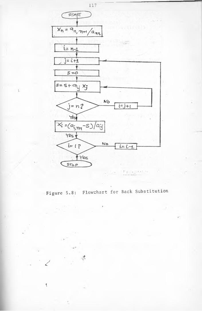
117
' - >Figure 5.8: Flowchart for Back Substitution
*V'
1

o o
118
C PROGRAMME LEAST SQUARE REGRESSIONDIMENSION MATRIX(2,3),A(2),SUM(2),RIGHT(2)REAL MATRIX,X,Y,A,W INTEGER MOPEN(9,FILE=’DATIN’,STATUS= ’OLD’)OPEN (7,FILE=’OUTPUT *,STATUS=’NEW1)WRITE(7,10)
10 FORMAT(5X,’ A2 ’ )C CLEAR ALL ELEMENTS THAT MAKE UP SUMMATION TERMS15 DO 30 1=1,220 S UM(I)= 0.030 RIGHT(I)=0.0C READ DATA AND FORM SUMMATION TERMS
M= 19 N = 2DO 50 J=1,M READ(9,200)X,Y,IF(Y.EQ.999)GO TO 350
200 FORMAT(F5.1,F8 .1)WRITE(*,100)X,Y
100 FORMAT(F5.1,F8 .1)W=ALOG(Y)DO 50 1=1,2
40 SUM(I)=SUM(I)+X**I50 RIGHT(I)=RIGHT(I)+W*(X**(1-1))C SET UP MATRIX
MATRIX(1,1)=M DO 70 1=1,2
60 MATRIX(I,3)=RIGHT(I)70 MATRIX(I,2)=SUM( I)
MATRIX(2,1)=MATRIX(1,2)WRITE(*,80)
80 FORMAT(2X ’NOW TO SUBROUTINE’)CALL GAUSS(MATRIX,A,N)WRITE(7,300)A(2)
300 FORMAT(F7.2)GO TO 15
350 C LOSE(7)STOP END
*******************************
Figure 5.9: Programme Least Square Regression
y V'
» 1

119
SUBROUTINE GAUSS(MATRIX, A , N)DIMENSION MATRIX( 2 , 3 ) , A( 2)REAL MATRIX,A
C ELIMINATION BEGINS HEREK= 1
400 I = K+1500 Z “ MATRIX( I , K) / MATRI X( K, K)
MATRIX( I , K ) =0 J = K+1
600 M A T R I X ( I , J ) = M A T R I X ( I , J ) - Z * M A T R I X ( K , J ) IF ( J . E Q . ( N + l ) ) GO TO 700 J = J+1 GO TO 600
700 I F ( I . EQ. N) GO TO 800t 1=1+1
GO TO 500800 I F ( K. EQ. ( N - 1 ) ) GO TO 900 '
K = K+1 GO TO 400
C BACK SUBSTITUTION BEGINS HERE900 A( N)=MATRIX( N, N+l ) / MATRI X( N, N)
I = N- 11000 J = I + 1
S = 02000 S = S + M A T R I X ( I , J ) * A ( J )
I F ( J . NE. N)GO TO 3000 A ( I ) = ( M A T R I X ( I , N + 1 ) - S ) / M A T R I X ( I , J )I F ( I . EQ. 1 ) GO T04000
- 1=1-1GO TO 1000
3000 : J=J+1GO TO 2000
4000 WRITE( * , 5 0 0 0 )5000 FORMAT( 2X * BACK FROM SUBROUTINE’ )
RETURN END
Figure 5.10: Subroutine Gauss
1

r120
01/01/84 SYSTEM UTILITIES - FILE DISPLAYA:/OUTPUT
. 0 9. 1 4 M Y e p x. 1 2 k'Ar ( P^^TT CXATDLVS.TPJ A L A R ^ Aj)• i o f v /A i f t o e > i : ( ^ e s < c ? G s / r v A L A R . e A ;. 0 8 K ) O M 6 A s A. 1 0 K I S U M U *
Figure 5.11: Results
SSlVERSITY
LIBRARY° F NAIROBI

121
5.2.5 Results and Observations
Figure 5.11 is a printout of the contents of the ouput file OUTPUT, resulting from running the programme 'Least Squares Regression' with the input data of Tables Figure 5.1. The values of A2 resulting from the regression analysis as described in Appendix 1 are given.
The resulting growth functions of the areas are given by the following expressions, for the 19 year period considered.
. .
c i
+ 0.09t V
(a) Nx(t) =le for Nakuru ASC area
C7 + 0.141(b) N2 ^ =
Le for Nyeri ASC area+ 0 . 1 2 t
(c) N3(t) = e 3 for Nairobi'sIndustrial area
c4 + 0 . lOt >
( d ) N4 (t) = e for Nairobi'sResidential area
C C+ 0 . 0 8 1 r'
( e ) NsCb) =be for Mombasa ASC area
c. + O.lOt(£) N6 (t) =
0e for Kisumu ASC area
*
The cons ta^tsV '
c^ vary depending on choice of* the y£ar to be considered as the base year (tQ) and does not affect the rate of growth, as illustrated in the figure below.

122
lnN.(t)"
1Xv y
If t~ is chosen as x then C- = C o i xIf t0 is chosen as y then = C
The slope of the graph is however unaltered. This illustrates the fact that the growth characteristics are fully described by the constant A2. As an investigation on whether the set of equation 5.8 represent the true growth functions the average deviation of values of N^(t) calculated from the equations from the actual data was determined. The r procedure followed is best explained by way of the following example. '
c2+0.14tv Consider t'h'e function 5.8b N9 (t) = e• c L
for Nyeri ASC area. If in 1968 equation 5.8b was used^to forecast the demand of telecommunications
• service in 1985, what would have been the percentage

125
error in the forecast from the actual data?.
In this example we let tQ = 1969 to determine c2
C2. . N2 (tQ) = e L = 1262.c? + 0.141
Thus N2 (1983) = e where t = 15= 1262 x e2 , 1
N2 (1983) = 10306
But the actual N2(1983) = 10064
Thus the error = 10506 — 10064 6 _ q .02 = 2110064
To obtain the average percentage error for 15 year forecasts using the equation the errors for the 1968 - 1982, 1967 - 1981, 1966 - 1980, 1965 - 1979 forecast periods were calculated and their mean taken.
The table below gives the percentage errors for each area obtained as explained above, for the indicated forecast periods.
1

124
^"'■'^Mrg.% error Area 5 Year Forecasts 10 Year Forecasts
1
15 Year Forecasts
1
Nakuru c*°
OO
CO . 5%
Nyeri 2 % 8% 2 %Mombasa 41 4% 6 %Kisumu 13% • 1 2% 5%Nairobi (I) 23% 2 1% 9%Nairobi (R) 1 2% 7% 8%
V ,
4t
Figure 5.12: Percentage error for various forecating periods

125
The table is interpreted as follows:-
Using the growth function of equation 5.7a to estimate demand at a time t years in Nakuru area for example the mean percentage error of the estimates is 8%
for 5 years forecasting periods, 8°& for 10 year forecasting periods and 5$ for 15 year forecasting periods.
From the contents of the table highest percentage errors occur at shorter forecasting periods, with the 15 year forecasting period giving relatively lower percentage errors. For this reason the 15 year forecasting period is considered optimum in the present exercise, giving errors ranging between 2% and 9%,
It is further observed from the table that larger errors are obtained from the Nairobi areas (both residential and industrial). The conclusion to be drawn here is that there are factors that affect telecommunications demand.in a manner that cannot be accommodated simply in the trend curves.This behaviour is expected when observing the graphs for the Nairobi area cases. It would therefore be
erroneous to forecast demand in these areas by considering historical data alone.

126
For the remaining areas it is safe to say that the demand growth is well approximated by the growth functions of equation 5 . 8 , . Indeed since forecasts are estimates, error margins of 2% to 6 %
in a period of 15 years can be considered acceptable.
1

r
127
5.3 FORECASTING OF DEMAND FOR TELECOMMUNICATIONS SERVICES
5.3.1 Forecasting Methods
There are many methods of forecasting thefuture development of telephone services in acountry, the principal ones being
(a) Intuitive forecasting - which is a systematic assessment based on subscriber surveys. These surveys are developed to produce forecasts of future demands.
(b) Normative forecasting - where it is assumed that there will exist some needs in the •: future which will affect the demand for telecommunications services.
(c) Comparison methods where the demand and growth characteristics of a particular area are forecasted on the basis of known historical patterns of another area.
(d) Trend methods - which depend on the•existenceof a sound d$ta base of past statistics. Past
/ •c trends are analysed from this data and used to forecast future growth. The assumption
t here is that future trends will have a predictable relationship with past trends.

128
5.3.1.1.- Trend Methods
In this work trend methods will be used for the
areas with adequate data with the aim of getting as realistic a picture as possible of the future demand for telephones. One simple approach is to calculate the future number of telephone instruments on the assumption that the annual percentage growth of telephones will be roughly the same in the future as in the past. This method has been used in the developed countries since World War I . The development of the telephone density in 15 countries is shown in Figure 5.13 from which it is apparent that this method could be applicable for short term prognosis (5 - 15 years) for those Western European countries which in 1925 had a density exceeding 1.5 per 100 inhabitants.
As previously discussed, the approximately straight line plots of Figure 5.2 for Nakuru,Kisumu, Nyeri and Mombasa leads to a conclusion\ > ^that a fairly constant rate of growth has been experienced in the previous (19 year) period. An extrapolation of these straight line graphs would extend this bahaviour to future years. Looking at graphs -.Figure 5.4 reveals that no saturation is expected within the- next say 10 - 15 years even if

\
129
pmrICO irtufeNtnU (k>9 U.4I4)
. * m . 3Figure 5.13: Telephone Density in 15 Countries
1

150
all demand for service was to be satisfied. Another factor to be considered is that the telephone penetration in the Kenyan network is still very low, which further confirms that saturation is not
eminent.
For these reasons _ meaningful forecasts of/
demand for telecommunications service in the four areas would be achieved by use of the equation set 5.3 . Forecast periods of both 10 and 15 years are used.
In our present application the 1990 and 1995 demand figures for the four areas were obtained as
follows. For 1990 demand figures
For a 10 year forecast period t is chosen as 1980i
CiS0 1^(1980) = e10a2 -
Thus ^(1990) Ni(1980) X e«> ‘ >
\ .For a 15 year forecast period
N-(1975K*
tQ is chosen as 1975
ciey
15a?•• • N . (1990) N±(1975) X e
1

151
Similarly the 1995 demand figures t = 1980
15a?and Ni(1995) = Ni(1980) X e
iThe table below gives these forecasted demand
figures.
DemandArea
10 years 1990
15 years 1990
1995
Nakuru 9795 10217 15371Kisumu 9490 11446 15631Nyeri 26971 25455 54273Mombasa 54962 55227 52051
V1

132
5.3.1.2 Comparison Method
This prognostic method implies that the
number of telephones in an area A is based on a comparison with the historical trend of a more developed area B.
i .
If for example the telephone density in area A is the same as it was in Area B x years ago, and the general telephone development is assumed to follow the same trend in the two areas, a prognosis can be made for the total number of telephones during the next x year period of area A, provided that reliable forecasts of the future growth of population are available. This method of forecast has been applied^ to the telephone density forecasts of France as compared to Sweden.
Figure 5a14 gives the telephone density developmentin France and Sweden. France had the same telephonedensity in 1962 as Sweden had in 1934. If the
\ %telephone density in France in the future follows the same development trend as it did in Sweden between f934 and 1962^ France is expected in 1990 to reach the Swedish telephone density standard of 1962.
4\
\

Figure
/
•14: Comparison Method^: Telephonedensity in Sweden 1890 - 1962 and in France 1921 - 1962
I

1 3 4
The disadvantage of this method when applied to two countries is that there are hardly any two countries which follow parallel development . In cases where two regions in the same country are considered it can be useful. In the present case the rate of growth in the five areas has been approximated to range from A2 = 0.08 to A2 = 0.14.Thus for a town area like Kericho for example for forecasting purposes a growth rate in this range could be used with little error anticipated.
1

135
CHAPTER SIX
CONCLUDING COMMENTS
It has been established that approximately 2490 of links connecting automatic exchanges are congested* Teletraffic experiences significant blocking on these routes resulting in users’ complaints. However it is also observed that there are some routes whete the circuit provision is far in excess of the requirements for the offered traffic. This is particularly so in the Coast Network where a route such as the Nairobi NSC - Mombasa GSC carries79.3 erlangs on 140 circuits. The Mombasa GSC - Malindi route carries 7.0 erlangs on 29 circuits, while the Malindi - Mombasa GSC route carries 7.4 erlangs
on 29 circuits. Noting that the coast network has two congested routes it is possible that this congest! 011
can be alleviated by redistribution of equipment frofl1 over provided to congested routes. In doing this cate should be taken to identify the available transmission system to accompany the available switching plant at both exchanges. Also the signallinS system employe'd on the over provided route must be thesame as that employed on the congested route.
+V'/* CA similar treatment is extendable to other
networks, and therefore to the Kenyan Telecommunications network’as a whole. Whereas it is not always possible

136
to increase telecommunications plant due to economic constraints, it is noted that by proper utilization and distribution of available plant congestion can be alleviated on some routes. By standardizing in future on Multi-Frequency Compelled Signalling (MFC) more equipment on different routes will be interchangeable thus allowing for easy redistribution
of equipment.
The demand for telecommunications services has not been successfully met by the Kenyan network. In some areas this is due to lack of sufficient switching equipment, while in other areas it is due to insufficient distribution line plant. By considering the effective capacity of switching equipment in an area, a conclusion is drawn as to the
reason for not satisfying demand.
A tabulation of effective capacity against demand for the years 1975, 1980 and 1983 in Mombasa, Nakiiru, Nairobi and Kisumu is shown
overleaf.
/c
4\

137
MOMBASA Effective Capacity Demand
1975 12,684 10.0081980 13,388 15,678
1983 20,790 19,431
NAKURU1975 2,080 2,5471980 5,322 5,982
1983 5,702 6,438
NAIROBI(RESIDENTIAL)
1975 3,000 3,7641980 5,200 5,0831983 7,000 8,166
NAIROBI(INDUSTRIAL)
1975 5,000 . 6,4901980 6 , 0 0 0 9,5651983 1 1 , 0 0 0 13,221
KISUMU >
1975 2,460 2,5551980 4,890 5,4891985 $6,640 4,754
1

138
In the Nairobi areas and Nakuru, unsatisfied demand is mainly due to insufficient switching equipment, whereas in Kisumu and Mombasa the demand results from inadequate distribution line plant.
Systematic and reliable demand forecasting minimises inadequate provision of telecommunication plant while ensuring that unnecessary plant is not installed. One such method giving realisting forecasts has been presented in this thesis. Although the method does not address itself to unforeseen circumstances such as sudden mushrooming of settlements brought about by newly constructed estates, affordability in the event of reduction of fees and increased demand due to better service availability among others, these can be taken care of by allowing a reasonable margin in the forecasts. These margins are dependent on the area, but bigger margins (101 - 15°&) should be used in highly industrial areas.
Further* studies in this field should include finding the relatfonship between the growth of demandfor telephones and indome per capita, as well as the
/relationship to population growth. Empirical research shows that a simple relationship exists
1

139
between these parameters. Since a large number of
economists today are engaged on studies of growth of national incomes it is possible to obtain relatively realistic figures about economic development decades ahead. This, in addition to the methods in this thesis would enable even more reliable forecasts on telephone demand provided that a realistic formula has been obtained for the relation between national income per capita and telephone demand growth. The forecasting period would also be increased.
In the present set up the traffic department is involved in collecting data and processing it by use of traffic tables. This method is tedious and time consuming involving many personnel. By adopting the methods presented in this thesis more time can be devoted by the personnel to the continuous observation of teletraffic thus improving the reliability of the data. The Data Processing Department can then run
the computer programmes on the main ICL computer situated at,the Kenya Post and Telecommunications Corporation (KR..& TC) headquarters building. As the KP & TC network is s>approaching a transitional .stage
j v'/
towai*ds digitization, it is an appropriate time to ensure that the shortcomings of .the existing analc/gue network are remedied. Digital Switching

140
systems are to be introduced in both urban and
rural areas, and sufficient telecommunications plant should be catered for. It is hoped that the findings and methods in this thesis will be adopted to achieve this.
4

141
Appendix I
METHOD OF LEAST SQUARES
1.1 Best possible fit principle
This is a method that is defined as a method of
compromising.
Consider a set of unknown parameter u:-
Measurement1
2
3
three measurements of an
Result u = a u = b u = c
Generally a f b f c. The problem at hand is thatof finding the true value of the unknown parameter u.This problem requires solving three equations withonly one unknown variable u'. Although this isimpossible a best possible fit may be found by
\ calculating the value of u which minimises the sum ofthe squared errors in the results.
* ‘The function of u to be minimised is:-
F(u) = (u - a) 2 + (u - b) 2 + (u - c) 21

142
The derivative
dF(u) _ ^- 2 ( u - a) + 2 ( u - b) + 2 (u - c)du
For a minimum
^ p
= 0 = 2 (u - a) + 2 (u - b) + 2 (u - c)du
u = a + b + c
Thus the arithmetic mean of the measurements is the best possible fit in the meaning of method of least squares.
1 • 2 Normal Equations
Consider now a case where the number of equations is greater than the number of unknown
's..variables.
allul + a1 2u2
II n i-* V * **
a2 1ul + -2 2 U2 C2
a31ul + a32^2 ii o
* c
To obtain a compromising solution the function which is the sum of the squared measurement errors is

143
minimised. That is:-
Culu2 ~ (allul + a12u2 ” ci) + (a21ul
a22u2 " c2 + a31ul + a32u2 " c3
is to be minimised.
ButdFCu^)
du., 2 (allui + ai2u? ” ^l^all + a21U1 +
2 2 u 2 " c2^a21 + “ a31ul + a52u2 “
c3)a31
dF(u1u2)du. 0 allul + alla12u2 ' allcl
+ a21u1 + a 2 1 a 22
* a31ul + a31a32u2 ' a31c3 = 0
or (all + a21 +a3X^ul + (alla12 + a21a22'+ a31a32^u2
= aU Cl + a21C2 + a31C3
Similarly from '
dF(u1u2)
.1 du*= 0 we get

144
ul(a12all + a22a21 + *32*31* + U2(a12 + *22 2 ^+ a32 ~ ^19^1 + a??c? + a**7C1 2 1 2 2 2 32 3
By solving these equations for u- and U2 the best compromise solution is found.
In our application there are 19 plottable
points for each station (wxixl^ 9 w2 1x2 ••• (W19X19 *The solution for the problem consists of determining the unknown parameters a- and a2 so that the straight line w = a- + a9x reproduces the 19plotted points as well as possible.
In order to fit the straight line to the 19 plotted points it is considered that everyone of the points satisfies the equation of the straight line.
Thus the system equations are:-
W1 = al. + a2xl
w2 = a j - + a2 x2
w3 = al +j a2x4\V k
<1 * 1' V
t I I
1 w19 = al + a2x19

145
This is a set of 19 equations with only two
unknowns; a- and a2 « In matrix form the system is:-
—1 "• —
1 X 1 w i
1 X 2 W2
1 X - w „$
1 x 4 w 4X
a 21 t 1
t 1 f
t f f
1 x 1 9 W1 9— J
By denotingr- — - —' 1 xi „ • wi
1x2
• v W2
» t II3• *
-aland c = 1
t t I
1 x19 w19— m mm
The system equation' in matrix form becomes
a y. u - . cK.
V
4\
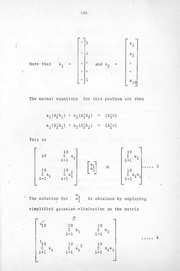
146
Note that
- —
1 1 x,1
1 1x2
t and A^ 1
1 i t
t 1 x19
The normal equations for this problem are then
1 A£Al) + a2 (AJA2) = (A{c)
1 A2A1^ + 3.^{A^A^) ■ W
This is
19
19i=iXi
19Z x. i = l
•r9 2 i=iXi
19iE=i ^
19£ x.w. i=i 1 1
The solution for a is obtained by employing\ * «simplified gaussian elimination on the matrix
*19
19Z x.i = l
• 19 Z x- i=i 1
19 . 2
19i£=l
19* xiWi i = l
4

147
REFERENCES
References for this thesis are in two groups. References 1 to 4 are particular to those portions marked in the text. References 5 to 19 are general references for larger portions of the work.
1. A Course in Teletraffic Engineering:Prepared by the Staff of Traffic Engineering Section, Planning Services Branch, Headquarter 1978.Telecom Australia.
2. V. Venuri: Modelling of Complex Systems -An Introduction.
3. Description of Methods of Making Forecasts. Swedish Telecomms. 1978,
• //4. Theory and Models For Traffic Forecasts.
Swedish Telecomms. 1978
«>

148
5. A. Elldin and G. Ling: Elementary TelephoneTraffic Theory.L. M. Ericsson Training Centre, Stockholm
6 . A. C. Bajpai, I. M. Calus and J. A. Fairley: Numerical Methods for Engineers and Scientists
7. Helm A.: Accuracy of Traffic Measurements.Telecom Australia, Traffic Engineering News Sheet No. 11. 1976
8 . D . Bear: Principles of TelecommunicationTraffic Engineering. Peregrinus, Stevenage, 1976
9. D. D. McCracken: A Guide to Fortran IVProgramming.

149
10. J. Ashcroft, R. H. Eldridge, R. W. Paulson,G. A. Wilson: Programming with Fortran 77,Department of Mathematics, University of Salford
1 1. T. 0. Wandera: Economic Optimisation ofAlternative Routes in the .East African Telephone Trunk Network.
, M.Sc. Thesis 1975
12. R. L. Freeman: Telecommunication SystemEngineering: Analog and Digital NetworkDesign.J. Wiley & Sons, N. Y. 1980
13. W. D. Gregg: Analog and Digital CommunicationJ. Wiley & Sons N. Y. 1977
. //14. Local Telephone Networks: International
Telecommunications Union, Geneva, 1968.
15. D. L. Schilling and H. Taub: Principles ofCommunication Systems.
*16. I.C.L. Technical Publications: Extended
Fortran (1900 Series)
«> . . .
&H1VERSITY O'F NAIROBI" library

150
17. Bright J.: A Brief Introduction toTechnology Forecasting.University of Texas in Austin U.S.A.,September, 1972.
18. Blair N.: Forecasting Telephone Traffic inthe Bell System.1976
19. General Systems Description: Type C400 CrossbarExchange, Hitachi Telecommunication Systems 1980.
s