Brigham Young University Brigham Young University

BYU ScholarsArchive BYU ScholarsArchive

Theses and Dissertations

2015-03-01

Temperature and Stress Effect Modeling in Fatigue of H13 Tool Temperature and Stress Effect Modeling in Fatigue of H13 Tool

Steel at Elevated Temperatures with Applications in Friction Stir Steel at Elevated Temperatures with Applications in Friction Stir

Welding Welding

Bradley Valiant Jones Brigham Young University - Provo

Follow this and additional works at: https://scholarsarchive.byu.edu/etd

Part of the Mechanical Engineering Commons

BYU ScholarsArchive Citation BYU ScholarsArchive Citation Jones, Bradley Valiant, "Temperature and Stress Effect Modeling in Fatigue of H13 Tool Steel at Elevated Temperatures with Applications in Friction Stir Welding" (2015). Theses and Dissertations. 4442. https://scholarsarchive.byu.edu/etd/4442

This Thesis is brought to you for free and open access by BYU ScholarsArchive. It has been accepted for inclusion in Theses and Dissertations by an authorized administrator of BYU ScholarsArchive. For more information, please contact scholarsarchive@byu.edu, ellen_amatangelo@byu.edu.

Temperature and Stress Effect Modeling in Fatigue of H13 Tool Steel at Elevated

Temperatures with Applications in Friction Stir Welding

Bradley Valiant Jones

A thesis submitted to the faculty of Brigham Young University

in partial fulfillment of the requirements for the degree of

Master of Science

Carl D. Sorensen, Chair Tracy W. Nelson C. Shane Reese

Department of Mechanical Engineering

Brigham Young University

March 2015

Copyright © 2015 Bradley Valiant Jones

All Rights Reserved

ABSTRACT

Temperature and Stress Effect Modeling in Fatigue of H13 Tool Steel at Elevated Temperatures with Applications in Friction Stir Welding

Bradley Valiant Jones Department of Mechanical Engineering, BYU

Master of Science

Tooling reliability is critical to welding success in friction stir welding, but tooling fatigue is not well understood because it occurs in conditions that are often unique to friction stir welding. A fatigue study was conducted on a commonly used tooling material, H13 tool steel, using constant stress loading at temperatures between 300°C and 600°C, and the results are presented. A model is proposed accounting for temperature and stress effects on fatigue life, utilizing a two-region Arrhenius temperature model. A transition in temperature effect on fatigue life is identified. Implications of the temperature effect for friction stir welding suggest that tooling fatigue life dramatically decreases above 500°C and accelerated testing should be conducted below 500°C.

Keywords: friction stir welding, H13 tool steel, Arrhenius model, elevated temperature fatigue, reliability, accelerated testing

ACKNOWLEDGMENTS

I am grateful for all the people that supported me and helped me through this process,

especially my family. Without the support and love of my wife, Kayla, I would not have been

able to complete this research. I am also indebted to Dr. Carl Sorensen for his continual

guidance, encouragement, and wisdom that helped me achieve more than I thought I was capable

of achieving. Lastly, I owe a special thanks to Denis Delagnes for sending me his doctoral

dissertation, which was invaluable in conducting this research.

TABLE OF CONTENTS

List of Figures ................................................................................................................................ v

List of Tables ............................................................................................................................... vii

1 Introduction ........................................................................................................................... 1

2 Background ........................................................................................................................... 3

2.1 Fatigue of FSW tooling ................................................................................................... 3

2.2 Literature on fatigue of H13 ........................................................................................... 4

3 Methodology .......................................................................................................................... 9

3.1 Equipment and materials ................................................................................................ 9

3.2 Procedure ...................................................................................................................... 11

3.3 Temperature calibration ................................................................................................ 11

4 Pilot study and experimental plan ..................................................................................... 15

5 Results and analysis ............................................................................................................ 20

5.1 Distribution form .......................................................................................................... 20

5.2 Stress effect modeling ................................................................................................... 22

5.3 Temperature effect modeling ........................................................................................ 26

5.4 Model assumptions ....................................................................................................... 30

6 Discussion ............................................................................................................................. 33

6.1 The loading method ...................................................................................................... 33

6.2 Comparison with other study results ............................................................................ 34

7 Conclusion ........................................................................................................................... 38

8 Future work ......................................................................................................................... 39

REFERENCES ............................................................................................................................ 40

Appendix A. Specimen drawing and manufacturing method ............................................. 42

iv

LIST OF FIGURES

Figure 2-1: Rate of cyclic softening varying with temperature. B is the cyclic softening rate (Engberg and Larsson 1988) .........................................................................................6

Figure 2-2: Basquin model fits of constant strain fatigue data from 200°C to 600°C. (Delagnes 1998) ...................................................................................................................8

Figure 2-3: Stresses from Delagnes’ Basquin fits of each temperature (Figure 2-2) at 10,000 cycles. (Delagnes 1998) ...........................................................................................8

Figure 3-1: Rotating-bending fatigue machine with mounted furnace and adjacent temperature controller. .......................................................................................................10

Figure 3-2: Thermocouple attached near minimum cross-section via fiberglass tape wrapping. ...........................................................................................................................12

Figure 3-3: Thermocouple attached near minimum cross-section via welding. ............................13

Figure 3-4: Temperature calibration plotting temperature measured on the specimen for thermocouples attached via wrapping with fiberglass tape (“wrapped”) and welding (“welded”), as a function of furnace setpoint. .....................................................14

Figure 4-1: Yield strength at elevated temperatures of H13 tool steel tempered to a hardness of 48 HRC (Philip 1990). ....................................................................................17

Figure 4-2: Basquin models were fit at each temperature for the pilot study data. .......................18

Figure 4-3: Stress estimates for N = 5 x 105 cycles and N = 106 cycles from the pilot study data. Inverse temperature and log stress scales were used in anticipation of an expected Basquin-Arrhenius model (see p. 23). Dashed lines correspond to temperatures chosen for the full study. ..............................................................................19

Figure 5-1: The data collected at 500°C and 816 MPa on (a) a Weibull probability plot and (b) a lognormal probability plot. The lognormal model provides a better fit. ............21

Figure 5-2: The Basquin model fit of the 400°C data showing the probability density function at the two stress levels. The fit line passes through the median cycles to failure at each stress level. .................................................................................................24

Figure 5-3: The Basquin model fit with the pooled stress effect as indicated by the constant slope across all temperatures. The line at 106 cycles identifies the stresses plotted in Figure 5-4 at each temperature. .........................................................................24

v

Figure 5-4: From the Basquin model fit with categorical temperature effects (equation 5) with the stress predicting a fatigue life of 106 cycles plotted for each temperature. (a) 95% confidence intervals are shown. (b) The stresses are plotted against inverse temperature. Individual labels are in °C. ...............................................................26

Figure 5-5: The two-region Arrhenius model relating the stress predicting a fatigue life of 106 cycles as a function of inverse temperature (see equations 9 & 12). Individual labels are in °C. ..................................................................................................................29

Figure 5-6:Studentized devianace residuals from the two-region Arrhenius model, (a) plotted by temperature and (b) plotted by predicted Ln(Cycles). Residuals from tests at 600°C are given as red diamonds. .........................................................................31

Figure 5-7: H13 does not have a “true” fatigue limit (the curve follows the dashed line). (Kazymyrovych 2010) .......................................................................................................32

Figure 6-1: (a) A log-stress-inverse temperature model (equation 13) applied to Delagnes’ 10,000 cycle stress estimates (see Figure 2-3). (b) The two-region Arrhenius model relating the stress predicting a fatigue life of 106 cycles as a function of inverse temperature (see equations 9 & 12). (Individual labels are in °C.) .....................................................................................................................................34

Figure A-1: Specimen Drawing (Image not to scale.) ...................................................................43

Figure A-2: Specimen manufacturing and heat treat process. .......................................................44

vi

LIST OF TABLES

Table 3.1: Furnace setpoint calibration comparing thermocouple attachment methods. (All temperatures are in °C) ...............................................................................................13

Table 4.1: Rotating bending fatigue life data from exploratory pilot study. .................................16

Table 5.1: Model effects from the pooled Basquin model with categorical temperature effects. (see equation 3). ‘L-R ChiSquare’ is the likelihood ratio test statistic and ‘Prob>ChiSq’ is the p-value for the given statistic. ...........................................................25

Table 5.2: Model effects from the combined Arrhenius-Basquin model. (see equation 7) ..........29

Table 5.3: The complete study data and the associated estimated median fatigue life (Predicted Cycles) from the Arrhenius-Basquin model (Equations 12) for the given temperature and stress. *After one specimen was run to failure at 500°Cand 764 MPa, the “low” stress level for 500°C was decreased to 746 MPa to ensure failures well beyond those at the “high” stress level. ........................................................30

Table 5.4: The scale parameter for the lognormal distribution from individual Basquin models fitted at each temperature. The scale parameter estimate for 600°C is about twice the size of the scale parameter at any of the other temperatures. ..................32

vii

1 INTRODUCTION

In friction stir welding, a high strength tool is plunged into the metal plates that are to be

welded, and under high torques the rotating tool uses friction to heat the plates sufficiently to

soften them, without melting the plates. The rotating tool then traverses the length of the seam,

blending the softened metal from the adjoining plates and thus forming a weld. The welding tool

geometry and materials are selected to withstand the extreme forces and temperatures inherent in

such a process. For the welding of steel, tools are commonly constructed of cermets, such as

tungsten carbide or pCBN (Rai, De, Bhadeshia, & DebRoy 2011). For the welding of aluminum,

steel tools are commonly used, since they are of a sufficient strength and are significantly more

affordable (Rai et al. 2011).

Tool reliability is important to weld quality, since tool failure can damage the weld. In an

effort to improve tool life there have been several studies conducted, most either studying the

effect of tool geometry on tool life (Prado 2003; Rai et al. 2011) or the effect of tool material

(Rai et al. 2011). Concurrent with these studies, it has been observed that tool life is affected by

welding parameters, but there have been no studies that have sought to quantify the effects of

welding conditions (specifically temperature) on tool life (not true in general). Prado et al.

suggested that another important factor that influences tool life is process parameters (Prado

2003), particularly welding speed, though their study did not investigate this factor in depth.

1

None of these studies go as far as attempting to predict probability of tool failure (a reliability

model), instead simply demonstrating that tool life is improved with a change in geometry or

material.

Just as there are currently no reliability models for friction stir welding tools, there

likewise have been no studies on the effects of welding temperature on tool life. One reason for

this is that under traditional weld speed and rotational speed control, weld temperature is free to

drift during welding. The development of temperature-controlled welding methodologies,

though, has brought the temperature effect into focus as a worthwhile point of study. This is of

particular importance since in tool life studies of welding speed and rotational speed effects,

these effects have always been confounded with the unknown temperature effect.

This study has sought to enable accelerated testing of friction stir welding tooling by

identifying a regime in which accelerated testing could be performed. Though this thesis has not

attempted to fill all of the identified opportunities, it has laid important groundwork by making

the following contributions:

1. A fatigue life distribution has been proposed for rotating bending fatigue of H13 at

elevated temperatures.

2. Temperature and stress acceleration of fatigue life has been modeled in the high cycle

fatigue (HCF) regime for H13.

3. A significant transition in fatigue behavior with temperature has been identified for H13

near 537°C, indicating a change in failure mode.

2

2 BACKGROUND

Fatigue of FSW tooling

Though studies on tool wear have made the most significant contribution to

understanding the effects of welding parameters (Fernandez & Murr 2004; Prado 2003), other

failure modes have been observed in research. In a study conducted by Nielsen (referenced in

Arora et al.), an H13 tool had its pin shear off during welding of Al 7075. Arora et al. attributed

this failure to operation conditions that had the tool stressed nearly to its maximum shear

strength, but Arora’s study did not seek to establish the mode of failure nor the life of the tool

under these conditions (Arora, Mehta, De, & DebRoy 2012). Similarly, Andrews found that a

tool (of unspecified material composition) lasted over 1 km in welding of 6XXX series

aluminums, but failed after only 2 m in welding 7XXX series aluminums (Andrews 2013). While

welding with an MP159 alloy tool in 16 mm 7075 plate, Colegrove & Shercliff also ran into tool

breakage (2003). All of these observed failures clearly suggest a potential fatigue failure

mechanism. The most significant study was performed at Hitachi, in which tool life was

calculated based on regular use conditions to be around 106 cycles. An accelerated stress test was

then conducted, resulting in failures around 103 cycles. Takai et al. indicated that the data was

found to compare favorably with data for rotating bending fatigue of the tool material at room

temperature. Unfortunately, without any of the actual data or the life-estimating reliability model

being given, and not knowing what tool material was used, the results of this study cannot be

3

explored further. Fortunately, the study has demonstrated that friction stir welding tools are

susceptible to fatigue and that fatigue modeling can accurately predict tool life (Takai, Ezumi,

Aota, & Matsunaga 2007). Before understanding the effect of welding parameters on fatigue life,

it is necessary to understand fatigue behavior of the base tool material outside of the context of

friction stir welding. For this study, the chosen material was AISI H13 hot work tool steel. H13

was chosen because is commonly used for FSW tools in the welding of aluminum alloys (Rai et

al. 2011).

Literature on fatigue of H13

H13 is part of a family of 5% chromium hot-work tool steels, of which H11 and H13 are

the most commonly used. H13 has a slightly higher vanadium content than H11 and thus is more

wear resistant, but this is traded for lower fracture toughness (Philip 1990). There is a large body

of literature on fatigue of H13 tool steel and because a common industrial use of H13 is in

forging dies, most of the studies on fatigue of H13 have sought to model those operating

conditions. As a result, studies on fatigue of H13, as well as the very similar H11 tool steel,

mostly focus on high strain isothermal cycling or thermomechanical cycling, thus leading to low

cycle fatigue (failure in less than 104 cycles) (Engberg & Larsson 1988; Velay 2005). Such

conditions, however, do not correspond to typical operating conditions for friction stir welding.

A study by Arora et al. found that the stresses in tools during the welding of AA6061 were

below the yield strength of H13, which would correspond to the high-cycle fatigue regime

(Arora et al. 2012). DebRoy, De, Bhadeshia, Manvatkar, & Arora specify that bending stresses in

tools can be as high 1500 MPa (2012) which is slightly above the ultimate strength of H13 at

room temperature (Philip 1990). Such a range of stresses clearly suggests that tool failures can

4

occur due to both high cycle fatigue and low cycle fatigue (LCF) when bending stresses

approach these high levels.

Despite the operational differences for the use of hot-work tool steels between forging

dies and friction stir welding, there are a number of important properties of H13 demonstrated by

these studies of low cycle fatigue. Velay et al. (2005) collected extensive fatigue data for AISI

H11 for strain-rate controlled, low cycle fatigue at temperatures from 300°C to 600°C. (This

temperature range contains the common friction stir welding temperatures for aluminum.) In

these fatigue tests, there were three observed crack initiation locations: “non-metallic inclusions

(NMI), lath boundaries, and grain boundaries of the initial austenitic microstructure.”

Quantification of these mechanisms led to the observation that NMI and lath boundary initiations

completely dominated grain boundary initiations below 400°C. Grain boundary initiation

“reach[ed] a proportion of 30% at 500°C, 65% at 550°C, and 90% at 600°C” (Velay 2005).

This observation of a transition in initiation mechanisms is significant because—though

Velay et al. were studying H11 steel—the transition in mechanism corresponds to an observed

transition in the rate of cyclic softening in a study of low cycle fatigue of H13 steel at elevated

temperatures conducted by Engberg and Larsson. In their study, isothermal high-strain fatigue

tests were conducted at 80, 300, 500, 600, and 750°C. Data from each of these tests was fit to a

cyclic softening model, and the rate of cyclic softening from the model for each temperature was

then graphed as a function of temperature (Engberg & Larsson 1988). The plotted “slopes” for

each temperature can be interpreted as the rate at which cyclic softening occurs per strain cycle.

Higher rates of cyclic softening correspond to shorter life, thus the higher the response, the fewer

cycles to crack initiation and failure. As can be seen in the plot from Engberg and Larsson

(Figure 2-1), they divided the softening into two regions, indicating that there is a sharp increase

5

in the cyclic softening when the temperature passes 430°C. This simply—yet significantly—

indicates that there is a transition in high strain (LCF regime) cyclic softening of H13 steel when

the operating temperature passes 430°C.

It should be noted that cyclic softening behavior was also observed by Velay et al. in

their study on H11 steel. They found that: “For the same strain ranges... An increase in

temperature implies a decrease of stress level, a more important cyclic softening intensity and

shorter lifetimes” (Velay 2005). Another important finding of this study was that there was no

evidence of a creep mechanism during fracture analysis, despite choosing some test conditions

purposely to induce creep. Though this study did not include H13 steel, the similarities between

the two alloys suggest that it could be expected that crack propagation in H13 steel at elevated

temperatures is similarly dominated by a fatigue mechanism, not a creep mechanism.

A very thorough study on fatigue of H11 was conducted by Denis Delagnes for his

doctoral thesis (1998). This study focused on the fatigue behavior around the transition from the

Figure 2-1: Rate of cyclic softening varying with temperature. B is the cyclic softening rate (Engberg and Larsson 1988)

6

low cycle fatigue regime (plastic strain dominated) to the high cycle fatigue regime (elastic strain

dominated). This research included an in-depth study of the cyclic softening behavior, and—

because the focus was on the LCF-HCF transition—Delagnes showed that cyclic softening is

only significant in the low cycle fatigue regime. Delagnes also studied the effects of hardness

and test temperature on fatigue life in this transition region. In examining the temperature effect

on fatigue, the majority of failure data in Delagnes’ study occurred between 4,000 and 50,000

cycles.

Basquin models (equation 1, where σa is the alternating stress, N is the fatigue life, and Ce

and p are model parameters) were fit by Delanges to each temperature (see Figure 2-2), giving an

independent stress-life relationship for each temperature. Then for each temperature, σa was

solved for given N = 10,000 cycles and plotted against temperature (see Figure 2-3). From this

plot, Delagnes identified a temperature transition in fatigue life behavior around 500°C. The

previously mentioned transition in dominant crack initiation locations with temperature were

given by Delagnes as the explanation for this transition in fatigue behavior. As this temperature

transition was only studied at the LCF-HCF transition, a primary aim of this thesis is to

determine whether such a transition exists in the high cycle fatigue range.

𝜎𝑎 = 𝐶𝑒 ∗ 𝑁𝑝 (1)

7

Figure 2-3: Stresses from Delagnes’ Basquin fits of each temperature (Figure 2-2) at 10,000 cycles. (Delagnes 1998)

Figure 2-2: Basquin model fits of constant strain fatigue data from 200°C to 600°C. (Delagnes 1998)

8

3 METHODOLOGY

To understand the effect of temperature on the fatigue life of H13, a rotating-bending

fatigue experiment was conducted using a cantilever-beam bending fatigue machine at several

temperatures. A pilot test was first conducted to estimate stress conditions that would yield

failures in the high cycle fatigue regime—traditionally considered to be above 104 cycles.

Following the pilot test, an in-depth study was conducted with 3 replicates at every test level.

Equipment and materials

The cantilever-beam rotating-bending fatigue machine used was a Fatigue Dynamics

RBF-200. The RBF-200 is capable of rotating specimens at up to 10,000 rpm and is calibrated to

provide a bending moment between 0 and 200 in-lbs. A built-in counter keeps track of the

accumulated cycles and upon specimen breakage, the load drops and shuts off the machine. For

temperature control, an electric resistance furnace was used in conjunction with a Love Controls

Model 25013 temperature controller.

9

Specimens were designed as directed in the RBF-200 user manual and in accordance with

ASTM E466, as far as permitted (Instruction Manual Model RBF-200; ASTM E466-07 2007).

The drawing used for manufacturing is found in Appendix A. All specimens were heat treated,

imbuing an average hardness of 48.7 HRC. The heat treatment followed these steps: specimens

were first austenitized at 1015°C for 1 hour, then air cooled; tools were then tempered for 1 hour

at 600°C, after which the furnace was turned off and allowed to cool with the parts inside. The

heat treatment resulted in warping of several of the specimens, but they were straightened at

elevated temperature (though below the tempering temperature) and any remaining runout was

believed to be insignificant due to the loading method1. As the final step in the manufacturing

process, the gauge section of each specimen was longitudinally ground to ensure a surface finish

1 Because the rotating bending fatigue machine applies its load to the specimen via a single downward force and does not restrict the movement of the load point (see Figure 3-1) the loading is able to maintain a constant force, despite possible movement due to runout from the specimen.

Figure 3-1: Rotating-bending fatigue machine with mounted furnace and adjacent temperature controller.

10

of 8 µ-in Ra. This was in accordance with ASTM E466 and helped minimize surface finish

effects on crack initiation (ASTM E466-07 2007).

Procedure

To ensure steady state temperature conditions, at the start of each testing period the

system was pre-heated by running the furnace at 700°C for 1 hour with a dummy specimen

installed. For each test, a thermocouple was secured onto the specimen just outside of the gauge

section using fiberglass tape. The specimen was then mounted within the collets of the rotating

bending fatigue (RBF) machine and the furnace closed around the specimen. The test specimen

was then preheated for 10 minutes at 20°C above the test temperature—to reduce the time to

achieve approximately steady state temperatures—following which the temperature was

decreased to the test temperature. The thermocouple attached near the gauge section was used to

monitor the stability of the actual specimen temperature, so as to gauge when an approximate

steady state temperature was reached. After specimen temperature had reached steady state, the

required load was applied and the RBF machine was turned up to 4500 rpm (±200 rpm to

prevent resonance). Upon failure, the number of cycles to failure was recorded.

Temperature calibration

Meaningful analysis of the study results was highly dependent on accuracy of the test

temperature. As indicated in Figure 3-2, the furnace controller received feedback via a

thermocouple mounted through the outer wall of the furnace, positioned near the heating coils.

Since the temperature at this position could not be assumed to coincide with the specimen

temperature, it was necessary to measure the specimen temperature and calibrate it against the

11

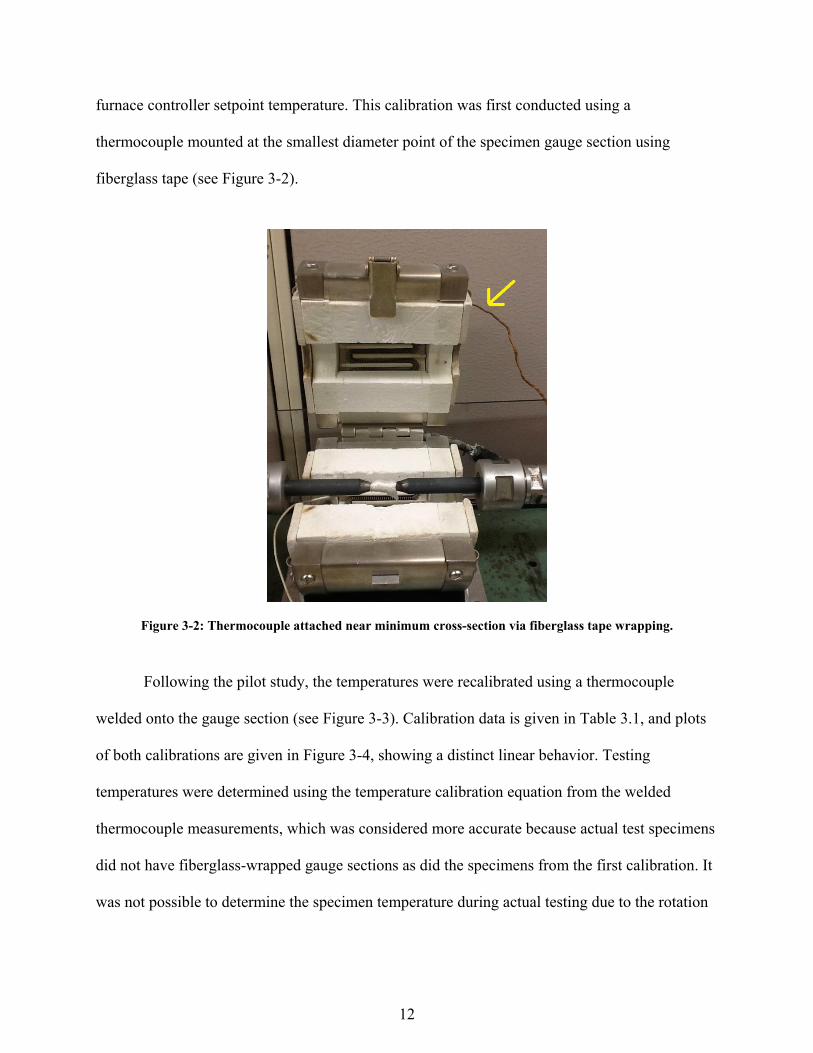
furnace controller setpoint temperature. This calibration was first conducted using a

thermocouple mounted at the smallest diameter point of the specimen gauge section using

fiberglass tape (see Figure 3-2).

Following the pilot study, the temperatures were recalibrated using a thermocouple

welded onto the gauge section (see Figure 3-3). Calibration data is given in Table 3.1, and plots

of both calibrations are given in Figure 3-4, showing a distinct linear behavior. Testing

temperatures were determined using the temperature calibration equation from the welded

thermocouple measurements, which was considered more accurate because actual test specimens

did not have fiberglass-wrapped gauge sections as did the specimens from the first calibration. It

was not possible to determine the specimen temperature during actual testing due to the rotation

Figure 3-2: Thermocouple attached near minimum cross-section via fiberglass tape wrapping.

12

of the specimen, but it was assumed that changes in temperature due to rotation were

insignificant. This assumption was justified by the fact that the during stationary heating, the

specimen temperature was observed to increase significantly whenever the controller relay was

on, thus suggesting that the radiative heat transfer dominated the convection heat transfer within

the furnace.

Table 3.1: Furnace setpoint calibration comparing thermocouple attachment methods.

(All temperatures are in °C)

Furnace Setpoint

Welded attachment

Fiberglass Wrapped Attachment

Welded/ Fiberglass Difference

403 300.2 296.8 3.4 487 399.8 391.5 8.4 571 499.5 486.1 13.3 614 550.5 534.6 15.9 656 600.3 581.9 18.4

Figure 3-3: Thermocouple attached near minimum cross-section via welding.

13

Figure 3-4: Temperature calibration plotting temperature measured on the specimen for thermocouples attached via wrapping with fiberglass tape (“wrapped”) and welding (“welded”), as a function of furnace setpoint.

14

4 PILOT STUDY AND EXPERIMENTAL PLAN

An exploratory pilot study was conducted seeking to a) verify the testing methodology;

b) see if the methodology gave repeatable results; and c) identify stresses at each temperature

that lead to failures in the HCF regime. Fifteen specimens were used across five different

temperatures, but a statistical experiment plan was not used, nor was the order of tests

randomized (Table 4.1). The tests were conducted at furnace temperatures of 398, 452, 518, 585,

and 667°C. With these furnace temperatures it was intended to obtain specimen temperatures of

300, 354, 419, 499, and 600°C, respectively, but the second calibration (see Calibration section

for details) showed actual specimen temperatures to be 304, 362, 438, 560, and 619°C. Despite

these differences, the results still provided useful information that was critical in designing the

full study.

The pilot testing resulted in the previously discussed testing methodology, and

repeatability of the results was taken as an indication of the soundness of the testing procedure

(see results for testing at 438°C for 807 MPa and 878 MPa in Table 4.1). A Basquin model was

fit to the results at each temperature, as was used by Delagnes for his S-N data (for Delanges

plot, see Figure 2-2). While there were only two data points collected at 304°C and 560°C, and

only 3 data points collected at 619°C, the Basquin model slopes at 304, 438, 560, and 619°C

were all very similar, which suggested a consistent stress effect across all temperatures. While

15

this temperature-independent stress effect was not modeled in in the pilot study, in the full study

such a temperature-independent stress effect was used in the fatigue life model and tested for

statistical significance.

When studying the effect of two different stresses on some response, a common approach

to understanding the effect of one stress on the response (assuming independence) is to hold the

other stress constant and look at the how the response varies as the free stress varies. This works

well in understanding the effect of mechanical stress on fatigue life, as demonstrated by the

Basquin model fits at each temperature. Unfortunately, to understand the effect of temperature

on life, stress cannot simply be held constant as temperature varies. This was demonstrated by

the testing that was done for 878 MPa at 438, 560, and 619°C: At this constant stress, the failure

at 619°C occurred in the LCF regime, whereas the same stress at lower temperatures led to

Table 4.1: Rotating bending fatigue life data from exploratory pilot study.

Pilot No. Temperature (°C) Stress (MPa) Cycles 1 425 930 362300 2 425 807 1007800 3 425 878 117300 4 425 878 140500 5 425 807 1111100 6 425 843 280700 7 540 878 56800 8 540 728 1071500 9 595 878 3800 10 595 728 83400

11 354 965 444000

12 300 1088 24400

13 300 1009 83800

14 595 685 54400

15 354 1009 624900

16

failures in the HCF regime. This is consistent with the known yield strength behavior of H13

(Figure 4-1, from Philip’s data): because the yield strength decreases dramatically above 425°C

(see Figure 4-1), a stress that caused only elastic strain below 425°C, thus leading to high cycle

fatigue—can induce plastic strain above 425°C—thus leading to low cycle fatigue. Delagnes’

study demonstrated that a temperature effect on fatigue could be studied by holding fatigue life

constant and seeing how mechanical stress varies as temperature varies : Obviously, fatigue life

cannot be held constant in actual testing, but by constructing a Basquin model from fatigue data

at two or more stress levels for each temperature, a stress can be calculated for each temperature

at the same cycles to failure, thus synthesizing this stress-temperature relationship at constant

fatigue life (see Figure 2-3 and the associated discussion on p. 7 to see how Delagnes’ did this).

Following Delagne’s method, the Basquin models from the pilot study (Figure 4-2) were

used to calculate the stress at N = 5 x 105 cycles and N = 106 cycles for each temperature. The

stresses at each temperature were then plotted as was done by Delagnes (see Figure 2-3), with

0

200

400

600

800

1000

1200

1400

1600

0 200 400 600 800

Yiel

d S

tren

gth

(M

Pa)

Temperature (°C)

Figure 4-1: Yield strength at elevated temperatures of H13 tool steel tempered to a hardness of 48 HRC (Philip 1990).

17

one difference: an inverse temperature scale and log stress scale were used on each respective

axis (Figure 4-3). These scales were used in anticipation of an expected Basquin-Arrhenius

model (see p. 23) that would be applied to the full study. From this plot, the stresses for the full

study were chosen for each of the full study temperatures. (For ease of comparing the complete

study results to the Delagnes’ results, the test temperatures for the complete study were chosen to

match the temperatures used by Delagnes: 300, 400, 500, 550, and 600°C.) Though the reader

may question this method of selecting tests stresses, the degree of accuracy of this process is not

important because all that was needed was to ensure that the high and low stress levels used in

the full study would place failures in the high cycle fatigue regime at every temperature,

preferably bracketing 106 cycles.

Figure 4-2: Basquin models were fit at each temperature for the pilot study data.

18

Figure 4-3: Stress estimates for N = 5 x 105 cycles and N = 106 cycles from the pilot study data. Inverse temperature and log stress scales were used in anticipation of an expected Basquin-Arrhenius model (see p. 23). Dashed lines correspond to temperatures chosen for the full study.

19

5 RESULTS AND ANALYSIS

In analyzing the fatigue data from the full study, these steps will be taken:

1. A lognormal distribution will be found to provide the best model of the distribution

2. A Basquin model with categorical temperature effect will be introduced and fit to the

fatigue data.

3. A continuous temperature effect (in the form of an Arrhenius model) will be proposed to

replace the categorical temperature effect.

4. A temperature region effect will be added to the model to account for a transition in

fatigue behavior.

5. Assumptions inherent to the model will be addressed an analyzed for their validity.

Distribution form

Because it is recognized that fatigue is a stochastic process rather than deterministic, the

models for fatigue life need to also model the variation in fatigue life. For this purpose,

parametric distributions are used to model the cycles to failure. Collecting nine data points at the

higher stress level for 500°C provided sufficient data to estimate the form of the distribution for

the cycles to failure. Fatigue data is traditionally fit using either a Weibull or lognormal

distribution (Veers, 1996).To determine which lifetime distribution provided a better model of

the data, both Weibull and lognormal distributions were fit to the 500°C data and goodness of fit

20

was compared. The relative likelihood of the lognormal distribution to the Weibull distribution

was found to be 3.00 (equation 2), indicating that the lognormal distribution is 3.00 times as

likely to minimize information loss due to modeling compared to the Weibull distribution. The

relative likelihood was calculated using AICc (Akaike Information Criterion with correction),

which is a measure of how effective a model is at capturing all the information available in a

dataset. The AICc for the Weibull and lognormal fits were calculated to be 252.7 and 250.5,

respectively.

exp (252.7 − 250.5

2) = 3.00 (2)

Figure 5-1(a) shows the 500°C data on a Weibull probability plot and (b) shows the data

on a lognormal probability plot. As demonstrated by the relative likelihood calculation, the data

plotted on the lognormal probability plot more closely follows the parameter estimate line than

the data on the Weibull plot follows the parameter estimate line. Neither the graphic evaluation,

nor the relative likelihood definitively indicate a “correct” model, they just indicate that the

lognormal distribution is more likely to capture more of the information in the data.

Figure 5-1: The data collected at 500°C and 816 MPa on (a) a Weibull probability plot and (b) a lognormal probability plot. The lognormal model provides a better fit.

(a)

(b)

21

Model fitting was conducted in the statistics program JMP using maximum likelihood

estimation (MLE). This method of model parameter estimation has a number of advantages over

least squares estimation. Generally, though, it provides a statistically more accurate estimate of

parameters and utilizes more of the information available in the data (Tobias & Trindade 2012).

In the MLE method, parameters are estimated by maximizing the likelihood function, which

represents the likelihood of the estimated parameters being the best fit, given all the data. The

value of the maximized likelihood function is called the likelihood.

The models for fatigue life presented in this study all follow a lognormal distribution,

unless otherwise stated, and therefore all modeled cycles to failure are the median cycles to

failure for the given conditions (which—for the lognormal distribution—is equivalent to the

mean of the natural logarithm of the cycles to failure). Though not presented with every model,

the scale parameter, σ—which accounts for the variance in fatigue life—is inherent to the

lognormal distribution and is given in this study where relevant. (Figure 5-2 provides a graphic

representation of the distribution and its variance.) For the lognormal distribution, the scale

parameter can be interpreted as the standard deviation of the natural logarithm of the cycles to

failure.

Stress effect modeling

A model was developed seeking to account for both the effect of stress as well as the

effect of temperature on the fatigue life of H13. To account for the stress effect, a Basquin model

(equation 3) was chosen, since this is a commonly used fatigue model (Veers 1996) and

Delagnes used this model for the S-N data in his H13 fatigue study (see equation 1). For this

study the Basquin model was used in the form of equation 3, where N is the cycles to failure

22

(actually the median cycles to failure or 50th percentile, since this follows a lognormal

distribution), Sa is the stress amplitude (σ is reserved to denote the lognormal scale parameter

instead of stress), and S0 is a normalization factor (1 MPa) to ensure correct units and C and b are

the model parameters. Note that this is just a rearrangement and re-parameterization of the

Basquin model as used by Delagnes (equation 1).

𝑁 = 𝐶 ∗ (𝑆𝑎

𝑆0)

𝑏

(3)

Equation 3 is only valid at constant temperature conditions. To evaluate the fit of the

Basquin model to the fatigue data across all temperatures, a categorical temperature effect was

added to the model. Treating the temperature effect as categorical allows the temperature effect

to be accounted for without assuming a form for the life-temperature relationship. The natural

logarithm of this model is expressed as

ln(𝑁) = ln(𝐶) + 𝑏 ln (𝑆𝑎

𝑆0) + 𝑎𝑇𝑖

(4)

where ‘aTi’ is the temperature effect for the ith temperature. Whereas equation 3 must be fit at

each temperature—and therefore gives different estimates of C and b (and the scale parameter, σ)

at each temperature—equation 4 provides a pooled estimate of C, b and σ across all

temperatures. The fit of the data at 400°C using equation 4 is depicted in Figure 5-2. To test the

statistical significance of the model, a likelihood ratio test was used. The likelihood ratio test

compares the likelihood of the given model with the likelihood of the same model, but with the

term being tested excluded; the test results in a p-value that indicates the probability that the

model with the effect is statistically the same as the model without the effect. Using this test,

both the stress effect and categorical temperature effects were significant (Table 5.1). Despite the

23

statistical significance of the model effects, the model is impractical since it ignores the

continuous nature of temperature.

Figure 5-2: The Basquin model fit of the 400°C data showing the probability density function at the two stress levels. The fit line passes through the median cycles to failure at each stress level.

Figure 5-3: The Basquin model fit with the pooled stress effect as indicated by the constant slope across all temperatures. The line at 106 cycles identifies the stresses plotted in Figure 5-4 at each temperature.

24

Table 5.1: Model effects from the pooled Basquin model with categorical temperature effects. (see equation 3).

‘L-R ChiSquare’ is the likelihood ratio test statistic and ‘Prob>ChiSq’ is the

p-value for the given statistic.

Effect L-R ChiSquare Prob>ChiSq Estimate ln(C) 16.10451 <0.0001 69.38544

b 11.30586 0.0008 -8.454308 Categorical

Temperature 35.65891 <0.0001

300 1.142873 304 0.130793 362 2.079574 400 1.010041 438 0.470175 500 0.276165 550 -0.23228 600 -0.46029 619 0.00

With the purpose of getting to a continuous temperature effect, equation 4 is rewritten to

express stress as a function of fatigue life and temperature (equation 5). As addressed in the pilot

study, it is impossible to conduct fatigue tests at constant stress across all temperatures, because

the temperature effects on fatigue would cause failures at high temperatures to occur in the low

cycle fatigue regime. By expressing stress as a function of temperature it is easier to examine the

temperature effect, since stress as a function of temperature can be plotted for a constant fatigue

life, as is done in Figure 5-4(a).

ln (𝑆𝑎

𝑆0) =

ln(𝑁) − ln(𝐶)

𝑏−

𝑎𝑇𝑖

𝑏 (5)

25

Temperature effect modeling

Figure 5-4(a) plots the stress-temperature relationship at 106 cycles to failure. It is

important to emphasize that the points on this plot do not represent actual failures, but rather are

points from solving equation 5 for each temperature, hence the 95% confidence intervals. Figure

5-4(b) plots the same data using inverse temperature on the abscissa. Inverse temperature was

used because it is consistent with an Arrhenius model of the temperature effect: Schuchtar used

an Arrhenius relationship to model the effect of temperature on fatigue crack propagation

(da/dN) in H13 (Schuchtar 1988) and the Arrhenius relationship is a commonly used model for

accelerating failures with respect to temperature in other reliability studies (Nelson, 1990; Tobias

& Trindade, 2012). The Arrhenius relationship can replace the categorical temperature effect by

substituting equation 6 into equation 4, giving equation 7, where T is the temperature in Kelvin,

R is the universal gas constant, and Q is the activation energy.

Figure 5-4: From the Basquin model fit with categorical temperature effects (equation 5) with the stress predicting a fatigue life of 106 cycles plotted for each temperature. (a) 95% confidence intervals are shown. (b) The stresses are plotted against inverse temperature. Individual labels are in °C.

(a)

(b)

26

𝑎𝑇𝑖=

𝑄

𝑅𝑇 (6)

Equation 7 is in log form, and can be expressed in its base form as:

𝑁 = 𝐷 ∗ (𝑆𝑎

𝑆0)

𝑏

∗ exp (𝑄

𝑅𝑇) (8)

Or equation 7 can be rearranged to give the relationship in equation 9, which could also be

considered a substitution of the Arrhenius relationship into equation 5.

ln (𝑆𝑎

𝑆0) =

ln(𝑁) − ln(𝐷)

𝑏−

𝑄

𝑏𝑅𝑇 (9)

Figure 5-4(b) provides a plot of the relationship from equation 9 at a constant fatigue life

of N = 106 cycles. The plot suggests that there is not a linear relationship between the natural log

stress and the inverse temperature; however, it can be seen that there are two approximately

linear temperature segments: one region being from 300°C to 500°C, the other region being

550°C to 619°C. To account for this two-region behavior, a temperature region indicator effect

(Gtemp) is added to the model along with an inverse temperature-temperature region interaction

effect, giving equation 10. The logarithmic form, equation 11, was the form used in JMP to

calculate the MLEs of the model parameters. By combining the temperature region indicator

effect and its associated interaction effect with their respective similar terms in the model,

equation 10 can be replaced with a piecewise equation—one portion for each temperature

region—in the form of equation 8. Thus the final two-region Basquin-Arrhenius model estimates

ln(𝑁) = ln(𝐷) + 𝑏 ∗ ln (𝑆𝑎

𝑆0) +

𝑄

𝑅𝑇 (7)

27

calculated using equation 11 are given in the form of the piecewise equation 12. The complete

study results are compared to the two-region Arrhenius model predictions for the given test

conditions in Table 5.3.

𝑁 = 𝐷 ∗ (𝑆𝑎

𝑆0)

𝑏

∗ exp(𝐺𝑡𝑒𝑚𝑝[0 1⁄ ]) ∗ exp (𝑄

𝑅𝑇) ∗ exp (

𝑄

𝑅𝑇∗ 𝐺𝑡𝑒𝑚𝑝[0 1⁄ ]) (10)

ln(𝑁) = ln(𝐷) + 𝑏 ∗ ln (𝑆𝑎

𝑆0) + 𝐺𝑡𝑒𝑚𝑝[0 1⁄ ] +

𝑄

𝑅𝑇+

𝑄

𝑅𝑇∗ 𝐺𝑡𝑒𝑚𝑝[0 1⁄ ] (11)

𝑁 = exp(72.32) ∗ (

𝑆𝑎

𝑆0)

−9.2

∗ exp (16031 J/mol

𝑅𝑇) 𝑇 < 537°C

𝑁 = exp(43.91) ∗ (𝑆𝑎

𝑆0)

−9.2

∗ exp (206944 J mol⁄

𝑅𝑇) 𝑇 > 537°C

𝜎 = 0.773

(12)

The two-region model identified 537°C as the transition temperature and indicated that

the change in activation energy was non-trivial. Table 5.2 provides the results of the likelihood

ratio tests from JMP, indicating that all model terms were significant. Figure 5-5 shows the two-

region Arrhenius model (taking the form of equation 9 to express stress as the dependent

variable) superimposed on the plot from Figure 5-4. It is important to note that data from the

pilot study was included in this analysis. Because the order of tests in the pilot study was not

randomized, it is possible that this data introduces some biasing into the model, but it was

assumed that the effect of any biasing would be outweighed by the increased accuracy of the

model.

28

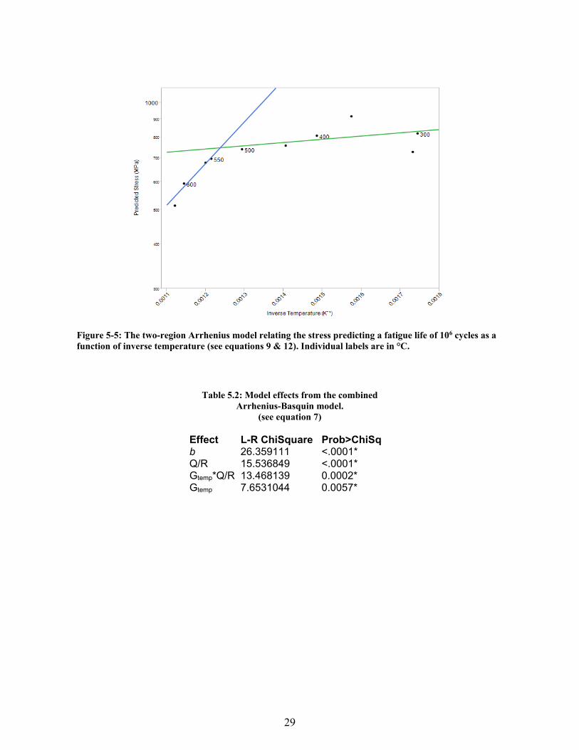
Table 5.2: Model effects from the combined Arrhenius-Basquin model.

(see equation 7)

Effect L-R ChiSquare Prob>ChiSq b 26.359111 <.0001* Q/R 15.536849 <.0001* Gtemp*Q/R 13.468139 0.0002* Gtemp 7.6531044 0.0057*

Figure 5-5: The two-region Arrhenius model relating the stress predicting a fatigue life of 106 cycles as a function of inverse temperature (see equations 9 & 12). Individual labels are in °C.

29

Model assumptions

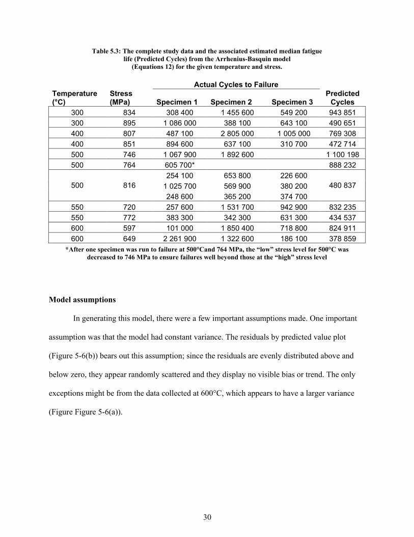
In generating this model, there were a few important assumptions made. One important

assumption was that the model had constant variance. The residuals by predicted value plot

(Figure 5-6(b)) bears out this assumption; since the residuals are evenly distributed above and

below zero, they appear randomly scattered and they display no visible bias or trend. The only

exceptions might be from the data collected at 600°C, which appears to have a larger variance

(Figure Figure 5-6(a)).

Table 5.3: The complete study data and the associated estimated median fatigue life (Predicted Cycles) from the Arrhenius-Basquin model

(Equations 12) for the given temperature and stress.

Actual Cycles to Failure Temperature (°C)

Stress (MPa) Specimen 1 Specimen 2 Specimen 3

Predicted Cycles

300 834 308 400 1 455 600 549 200 943 851 300 895 1 086 000 388 100 643 100 490 651 400 807 487 100 2 805 000 1 005 000 769 308 400 851 894 600 637 100 310 700 472 714 500 746 1 067 900 1 892 600 1 100 198 500 764 605 700* 888 232

500 816 254 100 653 800 226 600

480 837 1 025 700 569 900 380 200 248 600 365 200 374 700

550 720 257 600 1 531 700 942 900 832 235 550 772 383 300 342 300 631 300 434 537 600 597 101 000 1 850 400 718 800 824 911 600 649 2 261 900 1 322 600 186 100 378 859

*After one specimen was run to failure at 500°Cand 764 MPa, the “low” stress level for 500°C was decreased to 746 MPa to ensure failures well beyond those at the “high” stress level

30

To further explore the observed variance 600°C a simple Basquin model was fit at each

temperature (equation 3). From these individual Basquin fits the estimated scale parameter at

600°C, σ = 1.14, was approximately twice the value at the other temperatures (see Table 5.4). A

possible explanation for this increased variation is that at 600°C the uncertainty of the applied

stress (which is assumed to be constant across all temperatures) is a greater portion of the applied

stress, since the applied stress decreased as temperature increased. Thus the uncertainty of the

applied stress became a larger contributor to the variance of the fatigue life. This explanation is

inadequate by itself though, because if this were the case, it would be expected to see a growth in

variance as temperature increases, which is not demonstrated in Figure 5-6(a).

(a)

(b)

Figure 5-6:Studentized devianace residuals from the two-region Arrhenius model, (a) plotted by temperature and (b) plotted by predicted Ln(Cycles). Residuals from tests at 600°C are given as red diamonds.

31

Table 5.4: The scale parameter for the lognormal distribution from individual Basquin models fitted at each temperature. The scale parameter estimate for 600°C is about twice

the size of the scale parameter at any of the other temperatures.

Temperature (°C) σ Estimate Lower 95% Upper 95% 300 0.5416 0.2352 0.8480 400 0.5959 0.2588 0.9331 500 0.4476 0.2685 0.6266 550 0.5644 0.2450 0.8837 600 1.1444 0.4969 1.7919

Another possible contributor to this increased variation is that at 600°C both stress levels

were very near the fatigue limit. Research by Kazymyrovych (2010) indicates that there is not a

“true” fatigue limit for H13 in the sense that below the fatigue limit life is not infinite, but there

is a transition to a no longer linear log-Stress-log-Life relationship as demonstrated by

Kazymyrovych’s plot in Figure 5-7. Operating near the fatigue limit would greatly increase the

variation of the time to failure, which would be consistent with the greatly increased variance

estimated at 600°C.

Figure 5-7: H13 does not have a “true” fatigue limit (the curve follows the dashed line). (Kazymyrovych 2010)

32

6 DISCUSSION

The loading method

Before comparing the results of this study with other published findings, it is important to

examine the experimental setup and discuss the differences and commonalities it has with other

studies. The Delagnes’ study (1998) has the most in common with this study, but there are

several key differences. The first is that his Basquin modeling was conducted on H11 with a

hardness of 42 HRC, compared to the H13 with an average hardness of 48.7 HRC used in this

study. Delagnes’ specimens were subjected to uniaxial stress, whereas this study used rotating

bending stress. In rotating bending loading, only the outermost surface is subject to the

maximum stress, while uniaxial fatigue subjects the entire cross-section to a uniform maximum

stress. The differences in loading necessarily imply fewer cycles to crack initiation in the

uniaxial loading, since the increased area under stress means there are more sites available for

crack initiation.

Takai et al. suggested that rotating bending loading is actually very similar to the loading

conditions experienced by FSW tools: “It is likely that a torsional load from the rotational torque

is applied on the actual tool in addition to that noted above [the bending load] but when the pin

fracture surface is observed the fracture is at a right angle to the central axis and therefore [it is

assumed]... the effect of torsional stress is small” (Takai et al. 2007). Based on Takai’s

33

observation of tool fracture surfaces, we are inclined to accept that the torsional stress effect is

small. In such a case, the rotating bending loading does a good job modeling the majority of the

actual loading conditions on the FSW tool.

Another important difference in the loading is that Delagnes used constant strain loading,

whereas this study used constant stress loading. Delagnes conducted constant strain cycling in

the LCF-HCF transition region. Because Delagnes’ tests were in this region, cyclic softening

occurred in his specimens, meaning that the stress actually decreased during his constant strain

tests (1998). In this study, testing was in the HCF regime meaning stresses were low enough that

no cyclic softening occurred.

Comparison with other study results

It is of note that the activation energy for the low temperature region is consistent with

activation energies calculated for H13 by Schuchtar (1988). In his study he was looking at crack

propagation rates of H13 at elevated temperatures between 300°C and 500°C, using an Arrhenius

Figure 6-1: (a) A log-stress-inverse temperature model (equation 13) applied to Delagnes’ 10,000 cycle stress estimates (see Figure 2-3). (b) The two-region Arrhenius model relating the stress predicting a fatigue life of 106 cycles as a function of inverse temperature (see equations 9 & 12). (Individual labels are in °C.)

(b)

(a)

34

modification of the traditional Paris crack growth equation. Schuchtar found activation energy of

two different variants of H13 to be 13,000 J/mol and 17,000 J/mol, which is relatively close to

the 16,031 J/mol activation energy identified in this study. The activation energy indicates how

much the cycles to failure changes with an associated change in temperature. Below 537°C, in

the low temperature region, when the inverse temperature decreases by 2.176E-5 K-1

(approximately a 10°C increase around 400°C) the fatigue life decreases by 4.1%. In the high

temperature region, above 537°C, when the inverse temperature decreases by the same amount

(approximately a 15°C increase around 550°C), the fatigue life decreases by 41.8%. The obvious

implication for friction stir welding is that this suggests tool reliability dramatically drops in the

high temperature region.

Because Delagnes’ Basquin model didn’t use a single stress effect across all temperatures

as was done in this study, the same evaluation cannot be made from his data about the

temperature effect on fatigue life, but it is possible compare the temperature effect on stress at a

constant life between the two studies. Delagnes didn’t attempt to model the temperature effect,

but graphically identified it as occurring around 500°C (see Figure 2-3). By replotting the data

from Figure 2-3 on log stress and inverse temperature axes, equation 13 can be fit to Delagnes’

estimates of stress leading to a fatigue life of 10,000 cycles (SN=10,000), for a high temperature

region and a low temperature region. It is important to remember that this is a fit of Delagnes’

modeled points (SN=10,000), and not Delagnes’ actual fatigue test data. Using this method, the

temperature transition is found to occur at 488°C.

ln (𝑆𝑁=10,000

𝑆0) = 𝑦 +

𝑀

𝑇 (13)

35

From the Delagnes’ fit (Figure 6-1(a)), below 488°C, when the inverse temperature

decreases by 2.176E-5 K-1 (approximately a 10°C increase around 400°C) the stress leading to a

median life of 10,000 cycles decreases by 0.28%. Above 488°C, when the inverse temperature

decreases by the same amount (approximately a 15°C increase around 550°C), the stress leading

to a median life of 10,000 cycles decreases by 4.90%. From this study’s two-region Arrhenius

model (Figure 6-1(b)), below 537°C, when the inverse temperature decreases by 2.176 E-5 K-1

(approximately a 10°C increase around 400°C) the stress leading to a median life of 106 cycles

decreases by 0.45%. Above 537°C, when the inverse temperature decreases by the same amount

(approximately a 15°C increase around 550°C), the stress leading to a median life of 106 cycles

decreases by 5.71%. Despite the differences in the transition temperatures, for the high

temperature and the low temperature region from both models, temperature effect on stress at a

constant life is very similar.

It is important to acknowledge that the transition in the Arrhenius temperature effect is

likely not abrupt, despite using an abrupt transition model in this study. The transition in

activation energy is possibly the result of the increase in grain boundary crack initiation

identified by Delagnes in his doctoral research (Delagnes, 1998) and quantified by Velay (Velay

2005) (see p. 5). The data indicates that the transition between the two linear regions is clearly

not as abrupt as the model indicates (Figure 6-1(b)), which is consistent with the gradual growth

in prevalence of grain boundary initiations. Taking into account the likely gradual nature of the

transition in temperature effect, it is possible that the transition observed at 104 cycles (modeled

as occurring at 488°C) and the transition observed at 106 cycles (modeled as occurring at 537°C)

are one and the same.

36

Having identified two regions of fatigue behavior, it is important to revisit some of the

model assumptions to see if they are still valid. When there is a transition in failure mode, the

variance of life distribution can often change (Hu, Barker, Dasgupta, & Arora 1992). The

constant variance used in the model is therefore brought into question. Such a transition in model

variance could also be a reason for the significantly higher variance in the data collected at

600°C. Despite this possible deficiency in the model, from the perspective of friction stir

welding, the most important conclusion is unaffected: fatigue life dramatically decreases at

temperatures above approximately 500°C.

37

7 CONCLUSION

This study has demonstrated that there is a large temperature effect in high cycle fatigue of H13

tool steel. Near 537°C there is a transition in temperature effect, and above this transition the

temperature effect on fatigue life is almost 10 times the size of the temperature effect below the

transition. The implication for friction stir welding is that accelerated testing of FSW tools

should be conducted below 500°C to stay in the same failure mode. This in turn suggests that a

temperature control methodology (such as the method suggested by Ken Ross (Ross 2012))

should be used to control welding to ensure temperatures stay below this safe limit. Though the

differences between this study and Delagnes’ study of constant strain fatigue of H11 in the

vicinity of fatigue life of 10,000 cycles present some uncertainties, the similarities in the results

suggest that the temperature effect transition is the same (approximately 500°C) for high cycle

fatigue (~106 cycles) and the low cycle to high cycle fatigue transition (~104 cycles). Thus, the

temperature effect transition can be assumed to be independent of mechanical stress, and friction

stir welding temperatures should be kept below the transition temperature, regardless of weld

speed or tool stress.

38

8 FUTURE WORK

For the consideration of tool fatigue of H13 tools in friction stir welding, this research has

already determined important constraints on welding temperatures, but to predict fatigue life of

in-use tools, a fatigue study should be carried out on actual tools. This study has provided a

foundation for predicting tool life based on bending stresses that will provide guidance for

selecting welding parameters in an actual tool fatigue study.

Since this study conducted bending on 0.200” diameter specimens, the fatigue life

relationships found herein are only useful for the same dimensions in bending fatigue, though the

activation energies for the temperature effect are valid regardless of geometric factors. An

important step in expanding these relationships to more friction stir welding tools would be to

determine a geometry relationship that accounts for the change in fatigue life associated with a

change in specimen/tooling diameter and stress concentration factors. With further research in

fatigue of friction stir welding tools, a foundation will be established for maximizing tool usage

while minimizing in-use tool failures, thereby reducing welding costs and making friction stir

welding a more attractive manufacturing method.

39

REFERENCES

Andrews, R. E. "Improvements in Friction Stir Welding Tool Technology." TWI Industrial Member Report Summary 1046. TWI, 2013.

ASTM E466-07. Standard Practice for Conducting Force Controlled Constant Amplitude Axial

Fatigue Tests of Metallic Materials. West Conshohocken, PA.: ASTM International, 2007.

Arora, A., M. Mehta, A. De and T. DebRoy. "Load Bearing Capacity of Tool Pin During Friction Stir Welding." International Journal of Advanced Manufacturing Technology 61, (2012): 911-920.

Colegrove, P. A. and H. R. Shercliff. "Experimental and Numerical Analysis of Aluminium

Alloy 7075-T7351 Friction Stir Welds." Science & Technology of Welding & Joining 8, (2003): 360-368.

DebRoy, T., A. De, H. K. D. H. Bhadeshia, V. D. Manvatkar and A. Arora. "Tool Durability

Maps for Friction Stir Welding of an Aluminium Alloy." Proceedings of the Royal Society A: Mathematical, Physical and Engineering Science 468, (2012): 3552-35700

Delagnes, Denis. "Comportement Et Tenue En Fatigue Isotherme D'aciers a Outils Z38 Cdv5

Autour De La Transition Fatigue Oligocyclique-Endurance." Doctoral, Ecole Nationale Supérieure des Mines de Paris, 1998.

Engberg, G. and L. Larsson. Elevated-Temperature Low Cycle and Thermomechanical Fatigue

Properties of Aisi H13 Hot-Work Tool Steel. ASTM, 1988. Text. Fernandez, G. J. and L. E. Murr. "Characterization of Tool Wear and Weld Optimization in the

Friction-Stir Welding of Cast Aluminum 359+20% Sic Metal-Matrix Composite." Materials Characterization 52, no. 1 (2004): 65-75.

Hu, J. M., D. B. Barker, A. Dasgupta and A. K. Arora. "Role of Failure-Mechanism

Identification in Accelerated Testing." In Reliability and Maintainability Symposium, 1992. Proceedings., Annual, 181-188, 1992.

40

"Instruction Manual Model RBF-200 Rotating Beam Fatigue Testing Machine. " Dearborn, Mich.: Fatigue Dynamics Inc.

Kazymyrovych, Vitaliy. "Very High Cycle Fatigue of Tool Steels." Doctoral, Karlstad

University, 2010. Nelson, Wayne. Accelerated Testing : Statistical Models, Test Plans and Data Analyses. New

York: Wiley, 1990. Philip, T.V. and T.J. MCaffrey. "Ultrahigh-Strength Streels." In Properties and Selection: Irons,

Steels, and High-Performance Alloys, 1, 430-448: ASM International, 1990. Prado, R. A. Murr L. E. Soto K. F. McClure J. C. "Self-Optimization in Tool Wear for Friction-

Stir Welding of Al 6061+20% Al2o3 Mmc." MATERIALS SCIENCE AND ENGINEERING A 349, no. 1/2 (2003): 156-165.

Rai, R., A. De, H. K. D. H. Bhadeshia and T. DebRoy. "Review: Friction Stir Welding Tools."

Science & Technology of Welding & Joining 16, (2011): 325-342. Ross, Kenneth A. "Investigation and Implementation of a Robust Temperature Control

Alogorithm for Friction Stir Welding." Brigham Young University, 2012. Retrieved from http://scholarsarchive.byu.edu/etd/3919 (3919)

Schuchtar, E. "Temperature Dependence of Fatigue Crack Propagation in Hot Work Die Steels."

Theoretical and Applied Fracture Mechanics 9, no. 2 (1988): 141-143. Takai, H., M. Ezumi, K. Aota and T. Matsunaga. "Basic Study of Friction Stir Welding Tool

Life-Investigation for Increase of Fsw Reliability." Welding International 21, no. 9 (2007): 621-625.

Tobias, Paul A. and David C. Trindade. Applied Reliability. 3 ed. Boca Raton, Fla.: CRC

Press/Chapman & Hall, 2012. Veers, P.S. "Statistical Considerations in Fatigue." In Fatigue and Fracture, 19, 295-302: ASM

International, 1996. Velay, V. Bernhart G. Delagnes D. Penazzi L. "A Continuum Damage Model Applied to High-

Temperature Fatigue Lifetime Prediction of a Martensitic Tool Steel." Fatigue and Fracture of Engineering Materials and Structures 28, no. 11 (2005): 1009-1023.

41

APPENDIX A. SPECIMEN DRAWING AND MANUFACTURING METHOD

42

Figure A-1: Specimen Drawing (Image not to scale.)

43

Figure A-2: Specimen manufacturing and heat treat process.

44