temperature measurement - piyush panchal home

TEMPERATURE MEASUREMENT

by N. Asyiddin

- BLANK PAGE -

TABLE OF CONTENTS

TEMPERATURE MEASUREMENT................................................................................................ 1

WHAT IS TEMPERATURE? ............................................................................................................... 1 UNITS AND SCALES OF TEMPERATURE ........................................................................................... 2

Temperature scales.................................................................................................................. 2 Temperature scales development ........................................................................................ 2

Triple Point ............................................................................................................................... 3 Absolute Zero temperature....................................................................................................... 3 International Practical Temperature Scale of 1968 (I.P.T.S. - 68) ........................................... 3 Conversions between Units...................................................................................................... 5

METHODS OF TEMPERATURE MEASUREMENT.................................................................................. 8

A. Non-electrical systems..................................................................................................... 8 Liquid-in-glass Thermometers.................................................................................................. 8 Filled System Thermometer ................................................................................................... 10 Bimetallic Element.................................................................................................................. 16 B. Electrical or Radiation systems .................................................................................... 18 Thermocouples..................................................................................................................... 18

Thermocouples development ............................................................................................. 18 Thermoelectric Laws........................................................................................................... 19 Cold-junction compensation ............................................................................................... 21 Thermocouple circuits......................................................................................................... 23 THERMOCOUPLE REFERENCE CHART......................................................................... 25

Resistance Temperature...................................................................................................... 27

Platinum RTD ..................................................................................................................... 28 Radiation Types (Pyrometer) .............................................................................................. 32

Emissivity ............................................................................................................................ 32 Thermal Radiation Pyrometry ............................................................................................. 33 Radiation Pyrometer Applications ...................................................................................... 33 Optical Pyrometers ............................................................................................................. 34

- BLANK PAGE -

TTEEMMPPEERRAATTUURREE MMEEAASSUURREEMMEENNTT Temperature is one of the most frequently used process measurements. Almost all chemical and petrochemical processes and reactions are temperature dependent. Not infrequently in chemical plant, temperature is the only indication of the progress of the process. Where the temperature is critical to the reaction, a considerable loss of product may result from incorrect temperatures. In some cases, loss of control of temperature can result in catastrophic plant failure with the attendant damage and possibly loss of life. There are many other areas or industry where temperature measurement is essential. Such applications include steam raising and electricity generation, plastics manufacture and moldings, milk and dairy products and many other areas of food industries. Then, of course, where most of us are most aware of temperature is in the heating and air-conditioning systems which make so much difference to people's personal comfort. For the understanding of temperature measurement it is essential to have an appreciation of the concepts of temperature and other heat related phenomena. This includes deformation of temperature, heat, specific heat capacity, thermal conductivity, latent heat and thermal expansion. Why we need to measure temperature? Safety :- To ensure that process temperature remains within the limits of plant design, so

damage does not occur to columns, separator, piping and rotating equipment by exceeding their safety limits. For example carbon steal piping becomes brittle if it is cooled below minus 20 °C. It loses its mechanical strength if it is heated above 450 °C.

Quality :- Providing a more uniform and predictable product quality under steady process

conditions. Control:- To achieve correct control of process where temperature is a critical parameter.

These temperature dependant process include distillation, metering and regeneration.

What is temperature? Temperature is broadly defined as ‘degree of hotness or coldness of a body or an environment’. In a narrower sense, temperature is ‘the degree of hotness or coldness referenced to a specific scale’. It is a name for some condition in matter which determines the direction and extent of transfer of the kind of energy called ‘heat’. Temperature is an expression denoting a physical condition of matter, just as are mass, dimensions and time. Heat is a form of energy associated with the activity of molecules of a substance. These minute particles of all matters are assumed to be in continuous motion which is sensed as heat. Temperature is a measure of this heat.

! !!!!!!!!!!!!!!!!!!!!!!!!!!!!!!!!!!!!!!!!!!!!!UFNQFSBUVSF!NFBTVSFNFOU!!!!!!!!!!!!!!!!!!!!!!!!btzjeejoAzbipp/dpn! 2!

Units And Scales of Temperature

Temperature scales The two fixed points for temperature scales are;

1. the lower fixed point or ice point – which is the temperature of ice, prepared from distilled water, when melting under a pressure of 760 mmHg (or 1 atm, or 101.325 kPa, or 14.67 psi). The pressure of the atmosphere does not have a great influence on the melting point, but the ice should be in the form of fine shavings and mixed with ice-cold water. For the ice point, is the temperature at which water and ice can exist together.

2. the upper fixed point, or steam point – which is the temperature of steam from pure

distilled water boiling point under a pressure of 760 mmHg in latitude 45°. The boiling point, tp of water at a pressure, p mmHg is given by the formula;

tp = 100 + 0.0367 (p – 760) – (p – 760)2 °C Temperature scales development Galileo invented the liquid in glass thermometer around 1592 in crude form. Isaac Newton (1642-1727) first suggested fixed points of reference between freezing water and boiling water. Danish astronomer, Ole Roemer (1644-1710) had an obscure scale based on the number 60, with fixed points including human body temperature (at 28°C instead of the correct 37°C) and salted ice and water. He was first to use alcohol in his open thermometers. A more well-known scale is by dutchman Daniel Gabriel Fahrenheit (°F) who observed the work of Roemer, used alcohol but improved it by sealing the tops of his thermometers. Alcohol has a few problems with its high expansion factor and it can cling to the tubes, so Fahrenheit started to use Mercury. He then redesigned the thermometer by compensating for the low expansion factor by using a bulb at the bottom of the tube with a smaller interior bore. By 1714, he had produced a mercury in glass thermometer vastly superior to anything before, the design of which has hardly altered to this day. The odd scale 32°F for freezing water and 212°F for boiling water was because of his trying to improve on the scale of Mr Roemer. North America still uses this scale. He also discovered that water boils at different temperatures depending on the atmospheric pressure. Another scale was by the frenchman Rene Ferchaunt Reaumur (°R) was based on the number 80. Freezing water was 0°R and boiling water was 80°R at 1 atmosphere. He used an alcohol/water mixture, and was the first to use the standards of freezing and boiling of water as his sole points. This scale was widely used in Germany and France. Mr. Anders Celsius (°C) of Sweden by 1742 had the 100° scale thermometer which we use today, except for one major difference; it was upside-down. He used 100°C as “ice point” and 0°C as boiling point. A frechman, Christin, had developed a 100° scale the correct way up, at the same time. In 1750, after Celsius sudden death, the scale was reversed and named after him anyway. It was named for a long time “Centigrade”, meaning hundredth degree, until after 1940.

! !!!!!!!!!!!!!!!!!!!!!!!!!!!!!!!!!!!!!!!!!!!!!UFNQFSBUVSF!NFBTVSFNFOU!!!!!!!!!!!!!!!!!!!!!!!!btzjeejoAzbipp/dpn!3!

Lord Kelvin (°K) a British thermodynamicist, named the absolute unit “Kelvin” (derived from the Celsius). The absolute scale Rankine was derived from the Fahrenheit scale. The Kelvin is the SI unit of temperature - abbreviation as “K” without any degree sign ( ° ). The degree of both scales is equal to 1/273.16 of the temperature interval between absolute zero and the triple point of water.

Triple Point The triple point of water, is simply a temperature/pressure combination where the states of ice, water, and water vapour can exist together. Both a solid and a liquid phase usually exist together; with a certain amount of vapour (may or may not be visible) depending on the temperature and pressure. The triple point of water occurs at 0.01°C at pressure of 4.6 mmHg (or equivalent to 0.6132829 kPa, or 0.08894916 psi)

Absolute Zero temperature Absolute zero temperature is a state where all molecular activity has ceased, it is the coldest state there is, at a temperature of –273.16°C, or 0 Kelvin. However, this temperature was determined by calculation (theoretical), up until now this temperature has not been attained.

International Practical Temperature Scale of 1968 (I.P.T.S. - 68) Scales are constructed by referring to the IPTS. The scale is based on a number of fixed points which can be accurately reproduced. There are 12 basic points and a number of secondary points. It was established in 1968 by international commission and revised in 1990. The defining fixed points are established by realising specified equilibrium states between phases of pure substances. These equilibrium The scale distinguishes between the International Practical Kelvin Temperature with the symbol T68 and the International Practical Temperature Scale with the symbol t68. The relationship between T68 and t68 is;

t68 = T68 − 273.15 K The size of the degree is the same on both scales being 1/273.16 of the temperature interval between absolute zero and the triple point of water (0.01°C). Thus, the interval between the ice point, 0°C and the boiling point of water, 100°C is still 100 Celsius degrees. Temperatures below 273.15 K (0°C) are expressed in Kelvin (K), and in Celsius above 0°C.


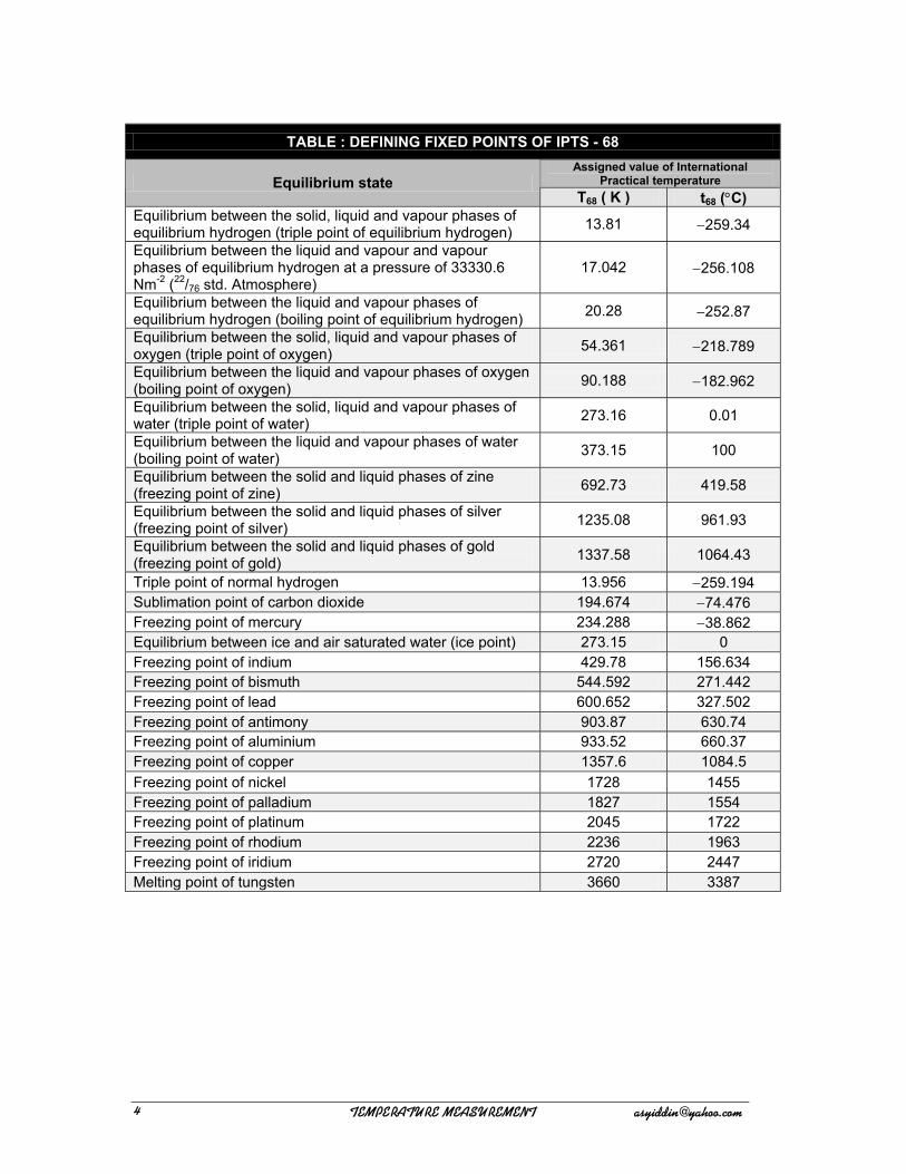
TABLE : DEFINING FIXED POINTS OF IPTS - 68 Assigned value of International

Practical temperature Equilibrium state T68 ( K ) t68 (°C)

Equilibrium between the solid, liquid and vapour phases of equilibrium hydrogen (triple point of equilibrium hydrogen) 13.81 −259.34

Equilibrium between the liquid and vapour and vapour phases of equilibrium hydrogen at a pressure of 33330.6 Nm-2 (22/76 std. Atmosphere)

17.042 −256.108

Equilibrium between the liquid and vapour phases of equilibrium hydrogen (boiling point of equilibrium hydrogen) 20.28 −252.87

Equilibrium between the solid, liquid and vapour phases of oxygen (triple point of oxygen) 54.361 −218.789

Equilibrium between the liquid and vapour phases of oxygen (boiling point of oxygen) 90.188 −182.962

Equilibrium between the solid, liquid and vapour phases of water (triple point of water) 273.16 0.01

Equilibrium between the liquid and vapour phases of water (boiling point of water) 373.15 100

Equilibrium between the solid and liquid phases of zine (freezing point of zine) 692.73 419.58

Equilibrium between the solid and liquid phases of silver (freezing point of silver) 1235.08 961.93

Equilibrium between the solid and liquid phases of gold (freezing point of gold) 1337.58 1064.43

Triple point of normal hydrogen 13.956 −259.194 Sublimation point of carbon dioxide 194.674 −74.476 Freezing point of mercury 234.288 −38.862 Equilibrium between ice and air saturated water (ice point) 273.15 0 Freezing point of indium 429.78 156.634 Freezing point of bismuth 544.592 271.442 Freezing point of lead 600.652 327.502 Freezing point of antimony 903.87 630.74 Freezing point of aluminium 933.52 660.37 Freezing point of copper 1357.6 1084.5 Freezing point of nickel 1728 1455 Freezing point of palladium 1827 1554 Freezing point of platinum 2045 1722 Freezing point of rhodium 2236 1963 Freezing point of iridium 2720 2447 Melting point of tungsten 3660 3387


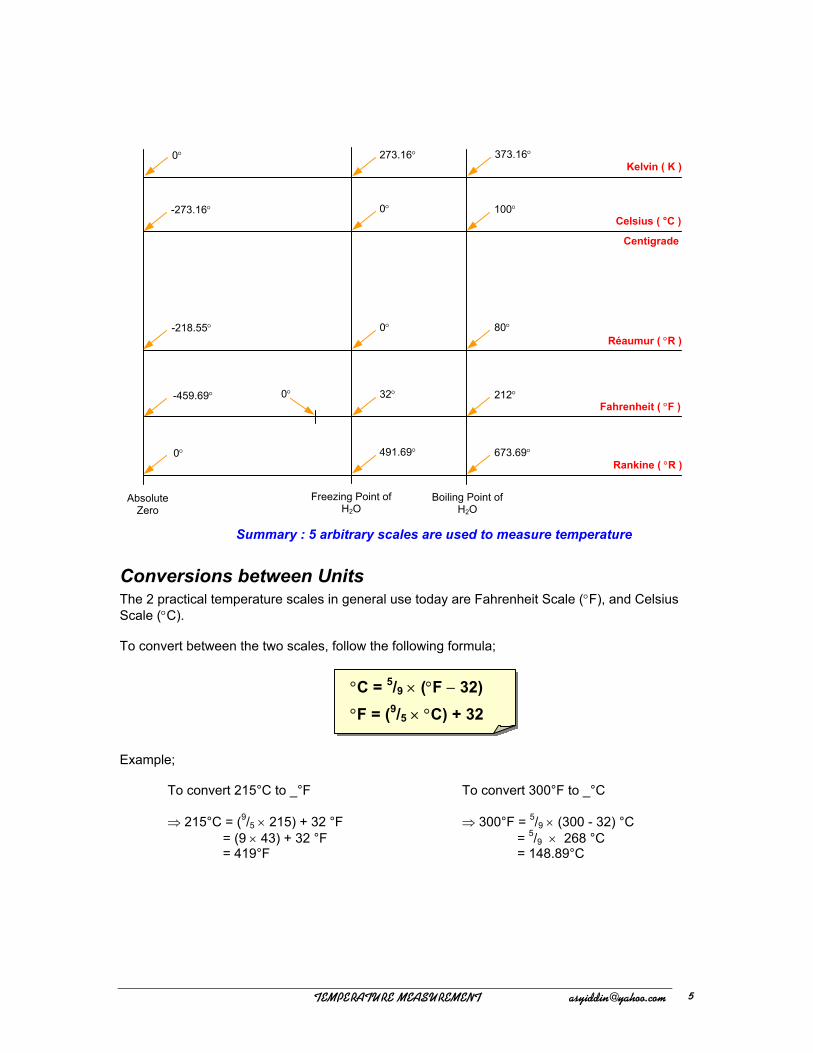
0°

673.69° 491.69°

212°

80°

32°

0°

100°

373.16°

0°

273.16°

Centigrade

Celsius ( °C )

Kelvin ( K )

Réaumur ( °R )

Rankine ( °R )

Fahrenheit ( °F )

0°

-459.69°

-218.55°

-273.16°

0°

Boiling Point of H2O

Freezing Point of H2O

Absolute Zero

Summary : 5 arbitrary scales are used to measure temperature

Conversions between Units The 2 practical temperature scales in general use today are Fahrenheit Scale (°F), and Celsius Scale (°C). To convert between the two scales, follow the following formula;

°C = 5/9 × (°F − 32)

°F = (9/5 × °C) + 32

Example; To convert 215°C to _°F ⇒ 215°C = (9/5 × 215) + 32 °F = (9 × 43) + 32 °F = 419°F

To convert 300°F to _°C ⇒ 300°F = 5/9 × (300 - 32) °C = 5/9 × 268 °C = 148.89°C


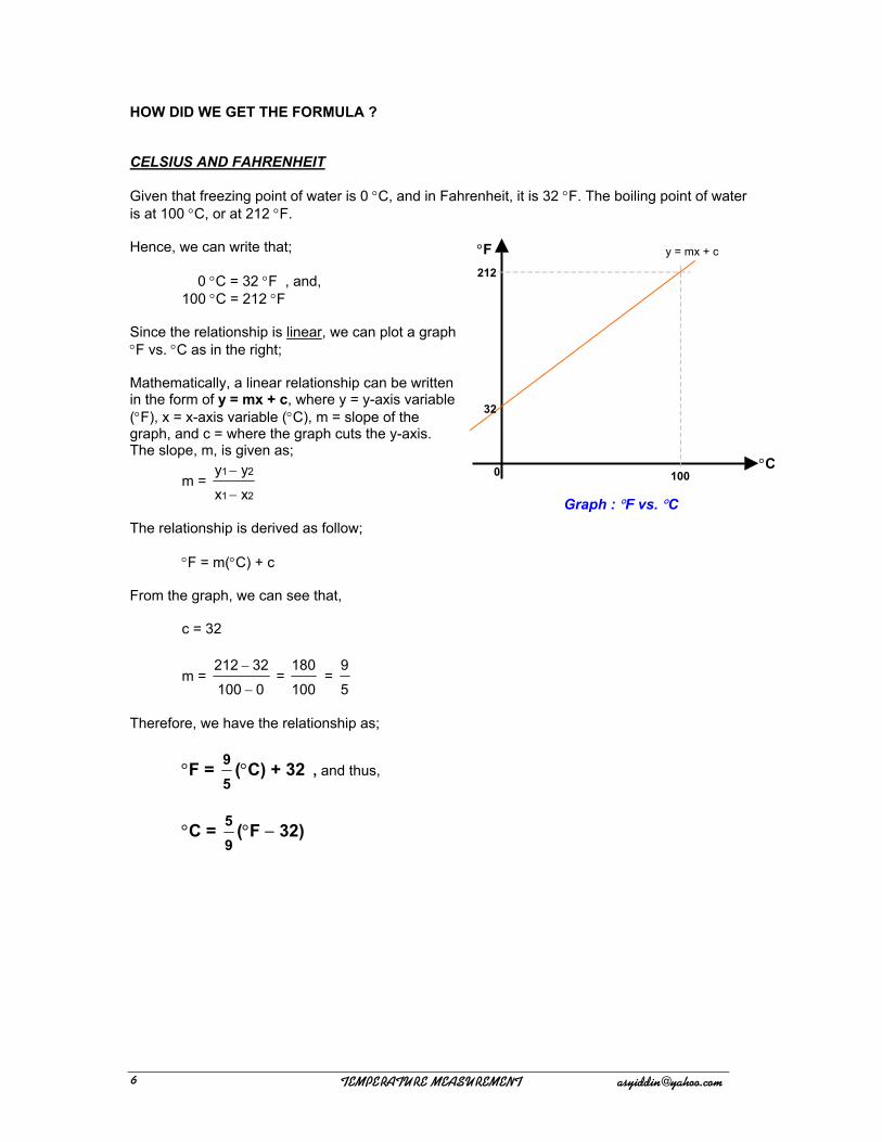
HOW DID WE GET THE FORMULA ? CELSIUS AND FAHRENHEIT Given that freezing point of water is 0 °C, and in Fahrenheit, it is 32 °F. The boiling point of water is at 100 °C, or at 212 °F. Hence, we can write that; y = mx + c

32

212

0 100

°F 0 °C = 32 °F , and, 100 °C = 212 °F Since the relationship is linear, we can plot a graph °F vs. °C as in the right; Mathematically, a linear relationship can be written in the form of y = mx + c, where y = y-axis variable (°F), x = x-axis variable (°C), m = slope of the graph, and c = where the graph cuts the y-axis. The slope, m, is given as;

°C m =

21

21

x xy y

−

−

Graph : °F vs. °C The relationship is derived as follow;

°F = m(°C) + c From the graph, we can see that,

c = 32

m = 0 100

−

− 32212 =

100180

= 59

Therefore, we have the relationship as;

°F = 59 (°C) + 32 , and thus,

°C = 95 (°F − 32)


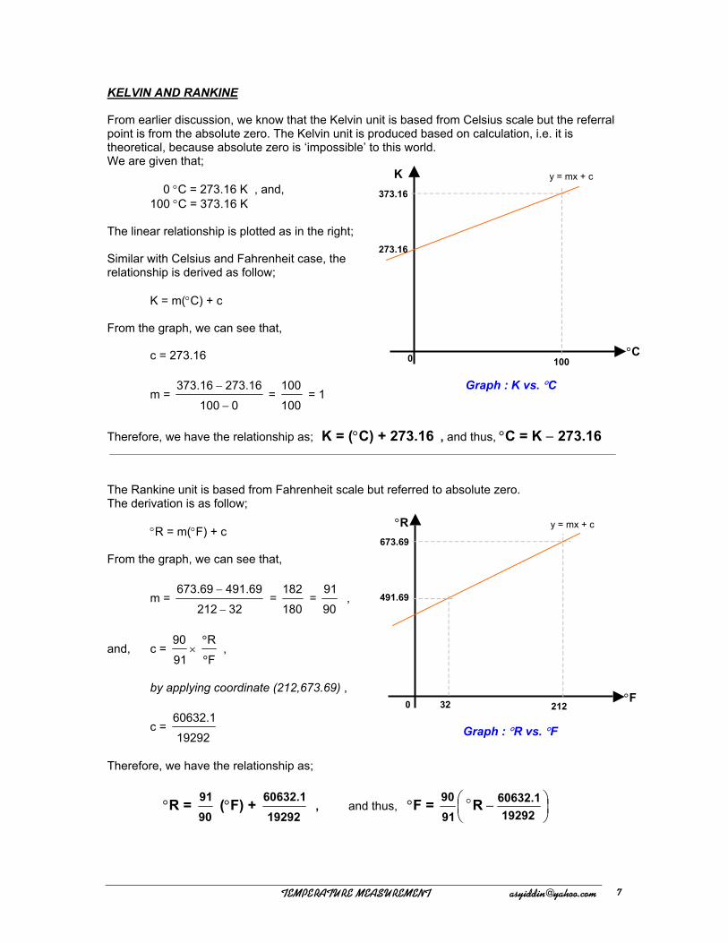
KELVIN AND RANKINE From earlier discussion, we know that the Kelvin unit is based from Celsius scale but the referral point is from the absolute zero. The Kelvin unit is produced based on calculation, i.e. it is theoretical, because absolute zero is ‘impossible’ to this world. We are given that;

y = mx + c

273.16

373.16

0 100

K 0 °C = 273.16 K , and, 100 °C = 373.16 K The linear relationship is plotted as in the right; Similar with Celsius and Fahrenheit case, the relationship is derived as follow;

K = m(°C) + c From the graph, we can see that,

°C c = 273.16

Graph : K vs. °C m =

0 100273.16 373.16−

− =

100100

= 1

Therefore, we have the relationship as; K = (°C) + 273.16 , and thus, °C = K − 273.16

The Rankine unit is based from Fahrenheit scale but referred to absolute zero. The derivation is as follow;

32

y = mx + c

491.69

673.69

0 212 °F

°R °R = m(°F) + c

From the graph, we can see that,

m = 32 212491.69 673.69

−

− =

180182

= 9091

,

and, c = 9190

× FR

°

° ,

by applying coordinate (212,673.69) ,

c = 19292

60632.1 Graph : °R vs. °F

Therefore, we have the relationship as;

°R = 9091 (°F) +

1929260632.1

, and thus, °F =

−

1929260632.1

9190 Ro


Methods of Temperature Measurement Heat cannot be measured directly, indirect approaches must be employed. Heat is only one form of energy, therefore it can be transferred or changed into other forms. If two bodies are at the same temperature, there is no exchange of heat. Some of the ways in which temperature may be inferred by the changes it causes are;

1. change in volume (pressure, viscosity, density, etc.) 2. a change in the electrical resistance 3. the voltage created at the junction of two dissimilar metals 4. the resonant frequency of a crystal 5. variations in the susceptibility of a paramagnetic salt in a magnetic field 6. the rate at which events take place

Generally, temperature measuring methods can be divided into 2 categories;

A. Non-electrical systems B. Electrical or Radiation systems

For expansion type of temperature sensor, observation that in a container (close-system), pressure and volume increase as temperature increase. The relationship between temperature, T, pressure, P, and Volume, V, can be expressed as; PV ∝ T ∴ PV = kT, where k is a constant.

A. Non-electrical systems The non-electrical systems are based on one of the following principles;

i. change in volume of liquid when its temperature is changed ii. change in pressure of a gas when its temperature is changed iii. change in vapour pressure when the temperature is changed iv. change in dimensions of a solid when its temperature is changed

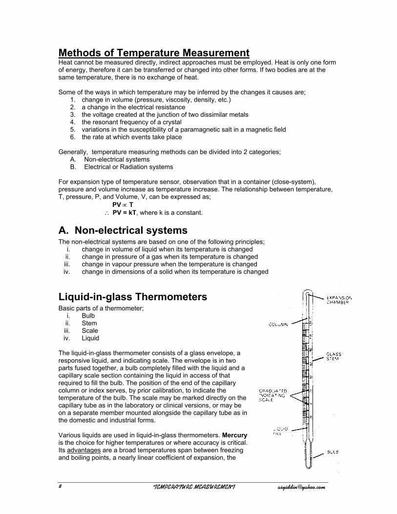
Liquid-in-glass Thermometers Basic parts of a thermometer;

i. Bulb ii. Stem iii. Scale iv. Liquid

The liquid-in-glass thermometer consists of a glass envelope, a responsive liquid, and indicating scale. The envelope is in two parts fused together, a bulb completely filled with the liquid and a capillary scale section containing the liquid in access of that required to fill the bulb. The position of the end of the capillary column or index serves, by prior calibration, to indicate the temperature of the bulb. The scale may be marked directly on the capillary tube as in the laboratory or clinical versions, or may be on a separate member mounted alongside the capillary tube as in the domestic and industrial forms. Various liquids are used in liquid-in-glass thermometers. Mercury is the choice for higher temperatures or where accuracy is critical. Its advantages are a broad temperatures span between freezing and boiling points, a nearly linear coefficient of expansion, the


relative ease of obtaining it in a very pure state, and its non-wetting of glass characteristic. The disadvantages are cost, relatively low coefficient of expansion and readability characteristics. For measurements below the freezing point of mercury (e.g. –39 °C), organic liquid such as toluene, aliphatic hydrocarbons, or organic phosphates are used. Advantages are low freezing point, superior readability to mercury when coloured with inert dyes, and lower cost. Disadvantages are lower boiling points, greater tendency to separate in the capillary, and wetting of glass characteristic.

Temperature range Fluid °C °F

Mercury −39 ~ 600 −38 ~ 11110 Mercury alloys −60 ~ 120 −76 ~ 250 Organic liquids −200 ~ 230 −328 ~ 450

The capillary above the liquid is generally filled with suitable gas. For the better grade thermometers, normally Dry Nitrogen is used. Air is often used in the less expensive mercury types as well as in the organic liquid-filled. Electric contact thermometers are generally filled with hydrogen. Maximum registering thermometers are sealed shut in a vacuous condition. Glass thermometers are made up of 3 classes;

i. Class A ii. Class B iii. Class C

! !!!!!!!!!!!!!!!!!!!!!!!!!!!!!!!!!!!!!!!!!!!!!UFNQFSBUVSF!NFBTVSFNFOU!!!!!!!!!!!!!!!!!!!!!!!!btzjeejoAzbipp/dpn! :!

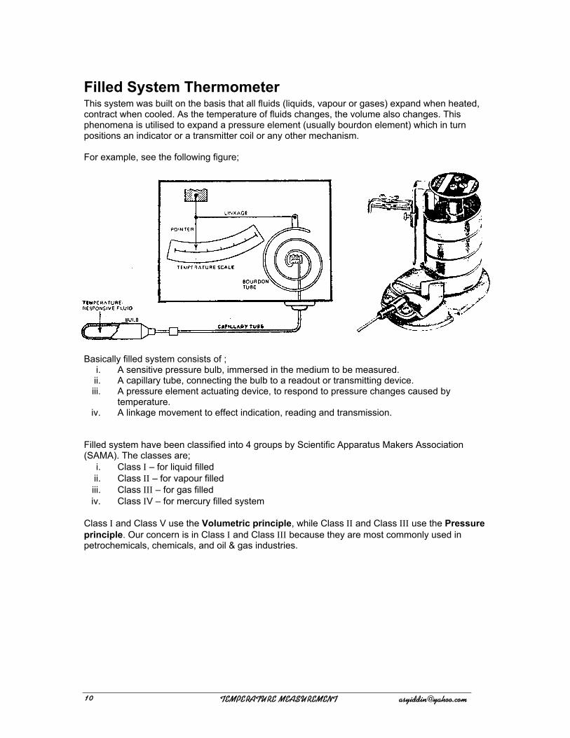
Filled System Thermometer This system was built on the basis that all fluids (liquids, vapour or gases) expand when heated, contract when cooled. As the temperature of fluids changes, the volume also changes. This phenomena is utilised to expand a pressure element (usually bourdon element) which in turn positions an indicator or a transmitter coil or any other mechanism. For example, see the following figure;

Basically filled system consists of ;

i. A sensitive pressure bulb, immersed in the medium to be measured. ii. A capillary tube, connecting the bulb to a readout or transmitting device. iii. A pressure element actuating device, to respond to pressure changes caused by

temperature. iv. A linkage movement to effect indication, reading and transmission.

Filled system have been classified into 4 groups by Scientific Apparatus Makers Association (SAMA). The classes are;

i. Class Ι – for liquid filled ii. Class ΙΙ – for vapour filled iii. Class ΙΙΙ – for gas filled iv. Class ΙV – for mercury filled system

Class Ι and Class V use the Volumetric principle, while Class ΙΙ and Class ΙΙΙ use the Pressure principle. Our concern is in Class Ι and Class ΙΙΙ because they are most commonly used in petrochemicals, chemicals, and oil & gas industries.

! !!!!!!!!!!!!!!!!!!!!!!!!!!!!!!!!!!!!!!!!!!!!!UFNQFSBUVSF!NFBTVSFNFOU!!!!!!!!!!!!!!!!!!!!!!!!btzjeejoAzbipp/dpn!21

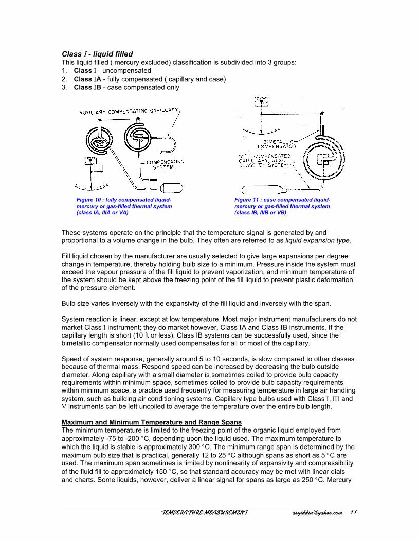
Class Ι - liquid filled This liquid filled ( mercury excluded) classification is subdivided into 3 groups: 1. Class Ι - uncompensated 2. Class ΙA - fully compensated ( capillary and case) 3. Class ΙB - case compensated only

Figure 11 : case compensated liquid-mercury or gas-filled thermal system (class IB, IIIB or VB)

Figure 10 : fully compensated liquid-mercury or gas-filled thermal system (class IA, IIIA or VA)

These systems operate on the principle that the temperature signal is generated by and proportional to a volume change in the bulb. They often are referred to as liquid expansion type. Fill liquid chosen by the manufacturer are usually selected to give large expansions per degree change in temperature, thereby holding bulb size to a minimum. Pressure inside the system must exceed the vapour pressure of the fill liquid to prevent vaporization, and minimum temperature of the system should be kept above the freezing point of the fill liquid to prevent plastic deformation of the pressure element. Bulb size varies inversely with the expansivity of the fill liquid and inversely with the span. System reaction is linear, except at low temperature. Most major instrument manufacturers do not market Class Ι instrument; they do market however, Class ΙA and Class ΙB instruments. If the capillary length is short (10 ft or less), Class IB systems can be successfully used, since the bimetallic compensator normally used compensates for all or most of the capillary. Speed of system response, generally around 5 to 10 seconds, is slow compared to other classes because of thermal mass. Respond speed can be increased by decreasing the bulb outside diameter. Along capillary with a small diameter is sometimes coiled to provide bulb capacity requirements within minimum space, sometimes coiled to provide bulb capacity requirements within minimum space, a practice used frequently for measuring temperature in large air handling system, such as building air conditioning systems. Capillary type bulbs used with Class Ι, ΙΙΙ and V instruments can be left uncoiled to average the temperature over the entire bulb length. Maximum and Minimum Temperature and Range Spans The minimum temperature is limited to the freezing point of the organic liquid employed from approximately -75 to -200 °C, depending upon the liquid used. The maximum temperature to which the liquid is stable is approximately 300 °C. The minimum range span is determined by the maximum bulb size that is practical, generally 12 to 25 °C although spans as short as 5 °C are used. The maximum span sometimes is limited by nonlinearity of expansivity and compressibility of the fluid fill to approximately 150 °C, so that standard accuracy may be met with linear dials and charts. Some liquids, however, deliver a linear signal for spans as large as 250 °C. Mercury

! !!!!!!!!!!!!!!!!!!!!!!!!!!!!!!!!!!!!!!!!!!!!!UFNQFSBUVSF!NFBTVSFNFOU!!!!!!!!!!!!!!!!!!!!!!!!btzjeejoAzbipp/dpn! 22

filled thermal systems may be used between -38 and 650 °C. Organic liquids freeze at a much lower temperature and are commonly used between -75 and 300 °C. Because of the higher expansivity, organic filled systems are more adaptable to short spans while the lower compressibility of mercury makes it easier to use on long spans. In either case, the minimum span is usually limited by the largest practical bulb size. Capillary and Case Compensation The non-metallic liquid systems are particularly vulnerable to errors resulting from capillary temperature changes because of the high expansivity of the fill. Only if the capillary volume is very small can these errors be ignored and a Class IB system used. See figure 11. To neutralize the capillary temperature error an auxiliary thermal system is employed. See figure 10. The mercury filled system may be compensated fully by an alternate method. This employs a capillary containing Invar wire which can, by proper selection of dimensions, cancel any net volume change due to the expansion of the mercury. It should also be noted that, because of low expansivity of mercury, Class VB systems can have capillary up to 50 ft with good performance. A VA system using compensated capillary, an ΙB, or VB often is preferred to a Class ΙA because of the relative simplicity of the construction, lesser vulnerability to abuse, and lower cost. Since the bourdon volume changes with measured temperature changes, the case compensation can be perfect at only bulb temperature. In practice, this compensation is adjusted to a specified tolerance with the bulb at midrange. This results in the thermometer being slightly overcompensated at range bottom and slightly undercompensated at range top. Attention must be paid to these details if precise measurements are desired. Class ΙΙ - liquid vapour system/vapour-pressure system Class ΙΙ systems utilise the vapour pressure of a volatile fill liquid as a pressure source to actuate the element. The system pressure will always be that occurring at the liquid-vapour interface. No compensation is necessary in vapour-pressure type systems. Care must be taken during manufacture to have the fill liquid, bulb, capillary and case at the same temperature. The are four subdivisions of this class; 1. Class ΙΙA :- designed for bulb placement in a process whose temperature always exceeds

the case ambient temperature (figure 12). 2. Class ΙΙB :- designed for bulb placement in a process whose temperature is always below

the case ambient temperature (figure 13). 3. Class ΙΙC :- designed for bulb placement in a process whose temperature can exist

periodically both above and below case ambient temperature, but whose temperature near case ambient temperature is unimportant (figure 14).

4. Class ΙΙD :- designed for bulb placement in a process whose temperature measurement,

when at case ambient is important, and which temperature can exist periodically both above and below ambient temperature (figure 15).

The fill fluid in a Class ΙΙA system is in a vapor state in the bulb and in a liquid state throughout the rest of the system (figure 12). The bulb must be sized to contain changes in volumes of the fill fluid in the bourdon, capillary and bulb due to ambient process temperature fluctuations while still maintaining the liquid-vapour interface within the bulb. Bulb length is therefore directly proportional to capillary length.


Figure 12 : Vapour-pressure thermal system (class IIA)

volatile liquidvapour

Figure 13 :Vapour-pressure thermal system (Class IIB)

Figure 14 :Vapour-pressure thermal system (Class IIC)

Figure 15 :Vapour-pressure thermal system (Class IID)

Long capillaries slow the response times of Class ΙΙ systems. The time constant (time, in seconds, necessary for the system to register 63.2 % of a step change) of a Class ΙΙA system is approximately 1 second for a 10-foot capillary but is about 10 seconds for long capillaries. Spans vary from 40 °F to 300 °F generally, with range limits between ambient and 550 °F . Class ΙΙB systems have all of the fill liquid contained within the bulb and, therefore, are not affected by ambient conditions (Figure 13). Bulb volume is generally less than those for Class ΙΙA systems. Response times of Class ΙΙB systems are essentially the same as for Class Ι systems. Class ΙΙB system spans vary from 40 °F to 300 °F generally, with range limits from ambient to about -430 °F .


Class ΙΙC systems, which can measure temperature above and below ambient but not at ambient, are constructed and filled so that the liquid part of the fill fluid exists in the capillary and bourdon when the bulb temperature is greater than ambient (Figure 14). When bulb temperature drops below ambient, the fill transfers into bulb (Figure 14). During the transfer the location of the liquid-vapour interface is undefined; therefore, system pressure does not represent an analog of bulb temperature. Span and range limits essentially encompass those of Class ΙΙA and Class ΙΙB systems. Bulb and instrument elevations must be virtually the same because of the fluid-vapor balance at the ambient crossover point. No compensation is available for elevation difference. Bulb volume is such that it will contain the volume of both capillary and bourdon and changes that occur in all portions of the system. It is usually larger than voltage than volumes for Class ΙΙA and Class ΙΙB systems. Response times are quite similar to Classes ΙΙA and ΙΙB. Transfer time when bulb temperature passes through ambient ranges from 5 minutes to an hour. Class IID systems are constructed such that the volatile fill fluid is sealed in the bulb by a nonvolatile liquid which also acts as a transmitting medium between vapor pressure in the bulb and the bourdon mechanism (Figure 15). Bulb size is usually the largest of all Class II systems due to the trap used to prevent the volatile fluid from ever reaching the capillary. The thermal mass of the trap itself and the use of the more viscous sealing fluid result in response times in the 5 to 10 -second range. Maximum and Minimum Temperatures The maximum temperature is limited by the critical point of the liquid employed and by the tendency of the most known organic liquids to change chemically at 316 C or higher. The minimum temperature is generally limited to approximately -40 C because of loss in reading sensitivity at lower temperature coupled with the requirement that the bourdon must be able to withstand the vapour pressure of the liquid at room (or possible shipping) temperatures. Capillary and Case Compensation The capillary of Class II systems is insensitive to temperature changes. It is necessary, however, that the capillary temperature of Class IIA systems, when the capillary and bourdon are filled with actuating liquid, should not be at a point that exceeds the bulb temperature. The internally contained fluid or vapour within the bourdon is also insensitive to temperature changes as above. However, the modulus elasticity will decrease with increasing temperature, causing a shift of only 1.5 to 2% for a 56 °C case temperature change. In most uses, this effect is not important and no compensation is provided.


Class ΙΙΙ - gas filled This system is defined by SAMA as "a thermal system filled with a gas and operating on the principle of pressure change with temperature change". The system is usually compensated for ambient temperature effects in one of the two ways : 1. Class ΙΙΙA: With a second thermal system minus the bulb, or an equivalent means of

compensation. 2. Class ΙΙΙB .With compensation means within the case only. Maximum and Minimum Temperature and Range Spans Gas thermal systems are able to cover the widest range of temperature of any of the filled systems. They are usually limited on the low side by the critical temperature of the gas used and on the high side of the bulb materials (commonly 5 K and 925 K). The maximum span is limited only by the above conditions of use and the nonlinearity due to mass flow from bulb. The minimum span is limited by the pressure at which the bourdon becomes overstressed. The gas system lends itself to use with a transducer with beading springs, making many more ranges, especially with short spans (25 K) available. Equation describes capillary temperature error in Class ΙΙΙ system;

( ) RTTVTVT∆T100VE

cbccb

2ccc

+⋅⋅

=

Where, Tc = mean capillary temperature, °R Tb = absolute temperature of bulb, °R ∆Tc = capillary temperature change, °F R = span, °F The following table is the summary or Guideline data for filled systems.

TABLE : GUIDELINE DATA FOR FILLED SYSTEMS Range Limits, °F Filled System

Classification (SAMA)

Fill Fluid Compensation Scale Lower Upper Overrange Bulb Elevation Errors

Ι Uncompensated −125 600 100%

ΙA Full −125 600 0 ~ 100% * ΙB

Liquid

Case

Linear Above −100°F −125 600 100%

Minor below 100 ft

ΙΙA Amb. 550 Minor below 100 ft

ΙΙB −430 Amb. None ΙΙC −430 to Amb. Amb. to 550 Not allowable ***

ΙΙD

Vapour Not required

Scale divisions increase

with temperature

increase −400 550

Almost always less than

100% Minor below 100 ft

ΙΙΙA Full −400 1500 None

ΙΙΙB Gas

Case

Linear Above −400°F −400 1500

100 ~ 300%** None

( SAMA has no Class ΙV ) VA Full −40 1000 VB

Mercury Case

Linear −40 1000

100% Minor below 25 ft

* depends on the bulb length ** depends on range *** bulb and measuring element must be at the same elevation


Bimetallic Element The bimetal thermometer, although widely used today, was not acceptable for industrial and laboratory use before about 1935. The fact that bimetal elements bend with temperature changes was observed over a century ago. These elements were then used for temperature correction in chronometers. The term “thermostatic bimetal” is defined as a composite material, made up of 2 or more different metals fastened together, which, because of the different expansion rates of the components, tends to change its curvature when subjected to change in temperature. There are 3 types of most commonly used in thermometers;

1. flat spiral 2. single helix 3. multiple helix

Multiple-helix Single-helix Spiral Bimetal strips are fabricated from 2 strips of different metals with different coefficients of thermal expansion, bonded together to form a cantilever. Typical metals are Invar and brass. See the following figure;

anchorage

anchorage

HOT

COLD brass

invar


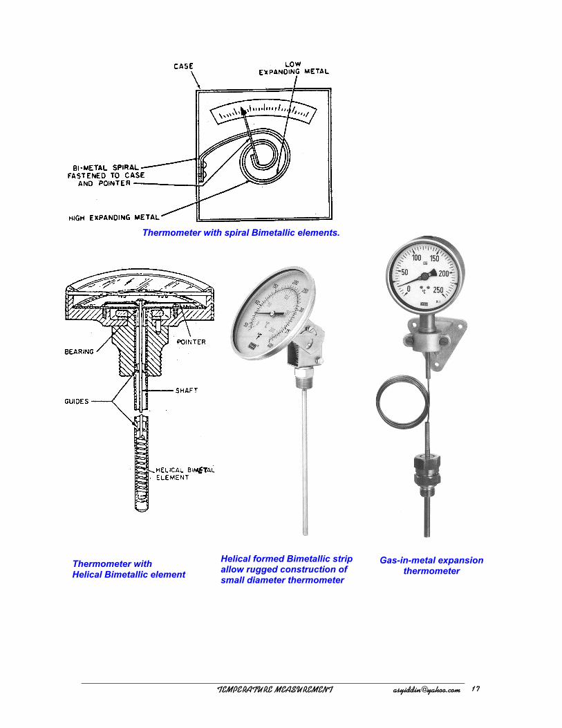
Helical formed Bimetallic strip allow rugged construction of small diameter thermometer

Gas-in-metal expansion thermometer

Thermometer with Helical Bimetallic element

Thermometer with spiral Bimetallic elements.


B. Electrical or Radiation systems The electrical systems are based on one of the following principles;

1. the Seebeck Effect (thermocouples). 2. change in resistance of materials as their temperature is changed. 3. the radiated energy emitted by an object is a measure of its temperature. 4. the brightness of an object or the energy radiated at a particular wavelength (in the

visible band) is a measure of its temperature.

Thermocouples Thermocouple is made up of two dissimilar metal conductors joined at one end, usually called the hot or detecting junction, and connected to some emf measuring instrument at the cold end of the conductors. Thermocouples development Seebeck Effect – Thermo-electricity In 1821, Seebeck discovered that if a closed circuit is formed of two metals, and the two junctions of the metals are at different temperatures, an electric current will flow round the circuit (i.e. voltage is induced). Seebeck arranged a series of 35 metals in order of their thermo-electric properties. In a circuit made up of any two of the metals, the current flows across the hit junction from the earlier to the later metal of the series (a portion of this series is as follow);

Bi-Ni-Co-Pd-U-Cu-Mn-Ti-Hg-Pb-Sn-Cr-Mo-Rh-Ir-Au-Ag-Zn-W-Cd-Fe-As-Sn-Te Peltier Effect In 1934, Peltier discovered that when a current flows across the junction of two metals, heat is absorbed at the junction when the current flows in one direction, and liberated if the current is reversed. The amount of that heat liberated, or absorbed, is proportional to the quantity of electricity which crosses the junction, and the amount liberated, or absorbed, when unit current passes for a unit time is called the Peltier Coefficient. The portion of the total emf of a thermocouple that exists because of a difference in potential a single section of wire or conductor having a temperature gradient is the Thomson emf. Thermocouple wires are chosen so that they will produce a large emf that varies linearly with temperature. Ideally chosen thermocouple material should have;

i. the Thomson emfs of the two wires additive in the circuit ii. Thomson emfs that vary directly with temperature iii. Peltier emfs that develop potentials at the hot junction that are in the same direction as the

Thomson emfs iv. Peltier emfs that vary directly with temperature v. Thermoelectric power as high as is possible


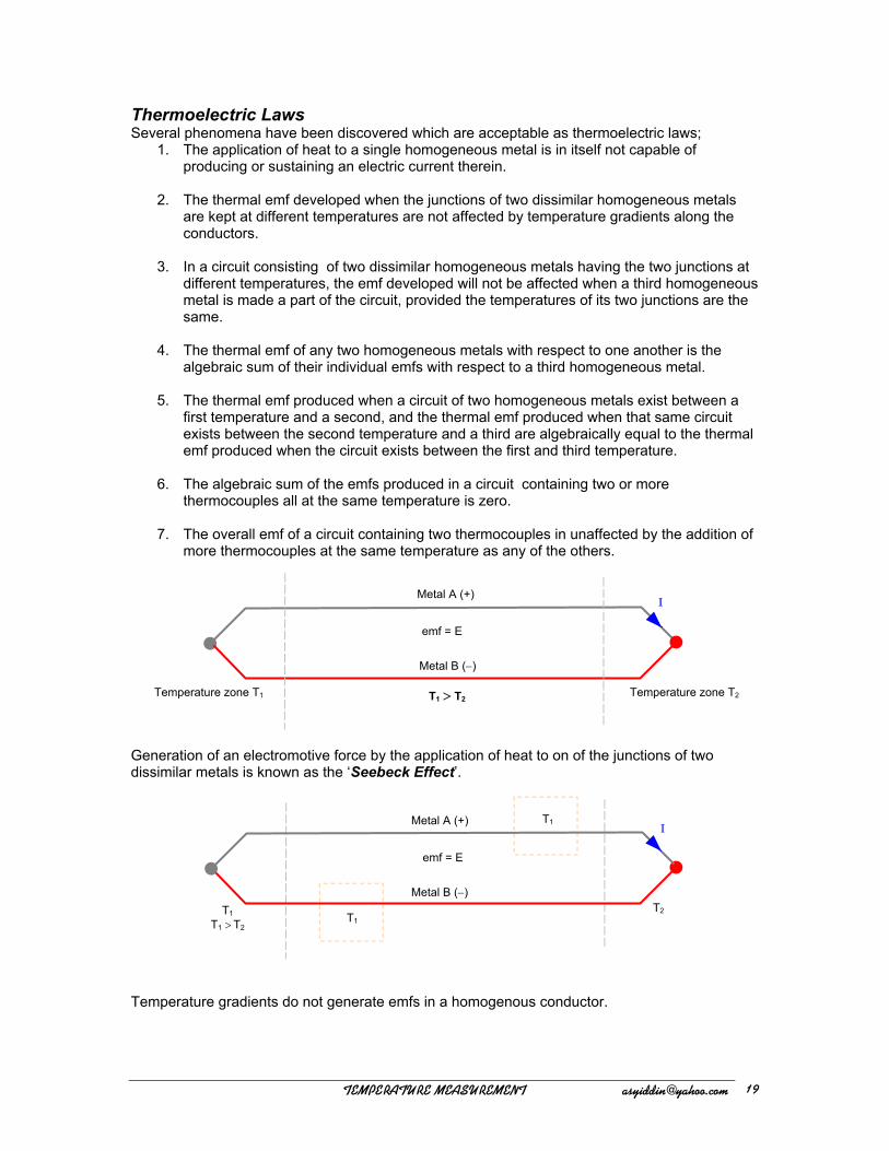
Thermoelectric Laws Several phenomena have been discovered which are acceptable as thermoelectric laws;

1. The application of heat to a single homogeneous metal is in itself not capable of producing or sustaining an electric current therein.

2. The thermal emf developed when the junctions of two dissimilar homogeneous metals

are kept at different temperatures are not affected by temperature gradients along the conductors.

3. In a circuit consisting of two dissimilar homogeneous metals having the two junctions at

different temperatures, the emf developed will not be affected when a third homogeneous metal is made a part of the circuit, provided the temperatures of its two junctions are the same.

4. The thermal emf of any two homogeneous metals with respect to one another is the

algebraic sum of their individual emfs with respect to a third homogeneous metal.

5. The thermal emf produced when a circuit of two homogeneous metals exist between a first temperature and a second, and the thermal emf produced when that same circuit exists between the second temperature and a third are algebraically equal to the thermal emf produced when the circuit exists between the first and third temperature.

6. The algebraic sum of the emfs produced in a circuit containing two or more

thermocouples all at the same temperature is zero.

7. The overall emf of a circuit containing two thermocouples in unaffected by the addition of more thermocouples at the same temperature as any of the others.

T1 > T2 Temperature zone T2 Temperature zone T1

emf = E

Metal B (−)

Metal A (+) Ι

Generation of an electromotive force by the application of heat to on of the junctions of two dissimilar metals is known as the ‘Seebeck Effect’.

Ι Metal A (+)

Metal B (−)

emf = E

T2 T1

T1

T1

T1 > T2

Temperature gradients do not generate emfs in a homogenous conductor.

! !!!!!!!!!!!!!!!!!!!!!!!!!!!!!!!!!!!!!!!!!!!!!UFNQFSBUVSF!NFBTVSFNFOU!!!!!!!!!!!!!!!!!!!!!!!!btzjeejoAzbipp/dpn! 2:

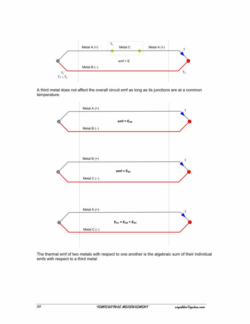
A third metal does not affect the overall circuit emf as long as its junctions are at a common temperature.

Ι Metal A (+)

Metal B (−)

emf = E

T2

T1 Metal A (+) Metal C

Ι Metal A (+)

Metal C (−)

EAC = EAB + EBC

emf = EBC

Metal C (−)

Metal B (+) Ι

emf = EAB

Metal B (−)

Metal A (+) Ι

T1

T1 > T2

The thermal emf of two metals with respect to one another is the algebraic sum of their individual emfs with respect to a third metal.


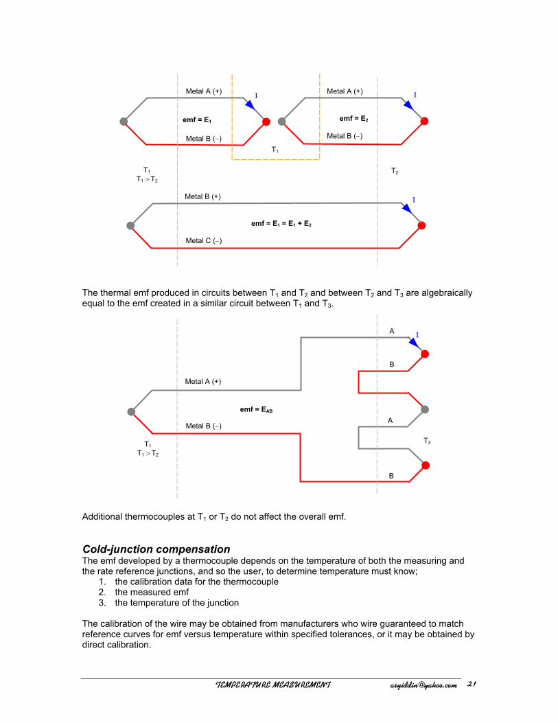
T1

T1 > T2

emf = E1 = E1 + E2

Metal C (−)

Metal B (+)

emf = E1

Metal B (−)

Metal A (+) Ι

Ι

Ι

Metal B (−)

emf = E2

T1

T2

Metal A (+)

The thermal emf produced in circuits between T1 and T2 and between T2 and T3 are algebraically equal to the emf created in a similar circuit between T1 and T3.

T1

T1 > T2

Ι

Metal A (+)

Metal B (−)

emf = EAB

B

A

B

A

T2

Additional thermocouples at T1 or T2 do not affect the overall emf. Cold-junction compensation The emf developed by a thermocouple depends on the temperature of both the measuring and the rate reference junctions, and so the user, to determine temperature must know;

1. the calibration data for the thermocouple 2. the measured emf 3. the temperature of the junction

The calibration of the wire may be obtained from manufacturers who wire guaranteed to match reference curves for emf versus temperature within specified tolerances, or it may be obtained by direct calibration.


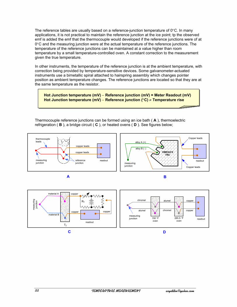
The reference tables are usually based on a reference-junction temperature of 0°C. In many applications, it is not practical to maintain the reference junction at the ice point; tp the observed emf is added the emf that the thermocouple would developed if the reference junctions were of at 0°C and the measuring junction were at the actual temperature of the reference junctions. The temperature of the reference junctions can be maintained at a value higher than room temperature by a small temperature-controlled oven. A constant correction to the measurement given the true temperature. In other instruments, the temperature of the reference junction is at the ambient temperature, with correction being provided by temperature-sensitive devices. Some galvanometer-actuated instruments use a bimetallic spiral attached to hairspring assembly which changes pointer position as ambient temperature changes. The reference junctions are located so that they are at the same temperature as the resistor.

Hot Junction temperature (mV) − Reference junction (mV) = Meter Readout (mV) Hot Junction temperature (mV) − Reference junction (°C) ≠ Temperature rise

Thermocouple reference junctions can be formed using an ice bath ( A ), thermoelectric refrigeration ( B ), a bridge circuit ( C ), or heated ovens ( D ). See figures below;

thermocouple leads

readout reference junction

measuring junction

copper leads

copper leads

measuring junction

OMEGA’S TRC

Copper leads

Copper leads

alloy A (+)

alloy B (−)

readout

A B

readout

RT

copper

copper

material A

material B

mea

surin

g ju

nctio

n

copper

T2

readout measuring junction

chromel

alumel chromel

alumel

copper

copper

150 °F oven

265.5 °F oven

C D


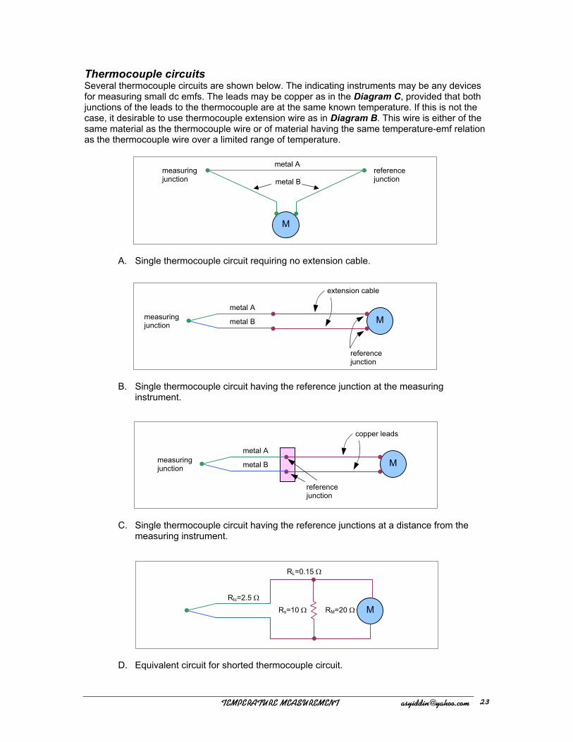
Thermocouple circuits Several thermocouple circuits are shown below. The indicating instruments may be any devices for measuring small dc emfs. The leads may be copper as in the Diagram C, provided that both junctions of the leads to the thermocouple are at the same known temperature. If this is not the case, it desirable to use thermocouple extension wire as in Diagram B. This wire is either of the same material as the thermocouple wire or of material having the same temperature-emf relation as the thermocouple wire over a limited range of temperature.

metal B

metal A measuring junction

reference junction

M

A. Single thermocouple circuit requiring no extension cable.

extension cable

metal B measuring junction

reference junction

metal A

M

B. Single thermocouple circuit having the reference junction at the measuring

instrument.

copper leads

metal B measuring junction

reference junction

metal A

M

C. Single thermocouple circuit having the reference junctions at a distance from the

measuring instrument.

RL=0.15 Ω

RM=20 Ω M Rs=10 ΩRtc=2.5 Ω

D. Equivalent circuit for shorted thermocouple circuit.


A B

reference junction

extension leads

+ −

+

+ −

−

mea

surin

g ju

nctio

ns

B A

B A B A

copper leads

selector switch − +

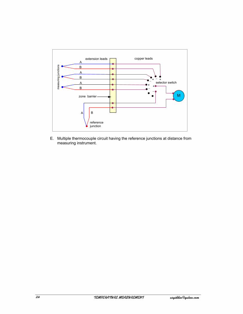
M zone barrier

E. Multiple thermocouple circuit having the reference junctions at distance from

measuring instrument.


JI

S C

161

0-19

81

NF

C 4

2-32

3

DIN

437

14

BS

1843

IEC

584

ANSI

/MC

96.

1

EMF

Ran

ge

1.79

2 ~

13

.820

mV

0 ~

37.0

79 m

V

-9.7

19 ~

76

.370

mV

-8.0

96 ~

69

.555

mV

-5.8

91 ~

54

.886

mV

-8.1

66 ~

53

.147

mV

-3.9

90 ~

47

.514

mV

-0.1

01 ~

21

.089

mV

-0.1

03 ~

18

.682

mV

-6.1

81 ~

20

.873

mV

-5.6

93 ~

34

.320

mV

Tem

p. R

ange

600

~ 18

20°C

0 ~

2316

°C

-250

~ 1

000°

C

-210

~ 1

200°

C

-200

~ 1

372°

C

-200

~ 9

00°C

-200

~ 1

300°

C

-20

~ 17

67°C

-20

~ 17

67°C

-250

~ 4

00°C

-200

~ 6

00°C

–ve

Leg

Pt–6

% R

h Pl

atin

um–6

% R

hodi

um

W–2

6% R

e (T

ungs

ten–

26%

Rhe

nium

)

Cu-

Ni

Cop

per-N

icke

l (a

lso

know

n as

C

onst

anta

n)

Cu-

Ni

Ni-A

l N

icke

l-Alu

min

ium

(m

agne

tic)

Also

kno

wn

as A

lum

el,

ther

mok

anth

al K

N, T

2, N

ial”

Cu-

Ni

Ni-S

i-Mg

Nic

kel-S

ilicon

-Mag

nesi

um

(als

o kn

own

as N

isil)

Pt

Plat

inum

Pt

Plat

inum

Cu-

Ni

Cu-

Ni

+ve

Leg

Pt–3

0% R

h Pl

atin

um–3

0% R

hodi

um

W–5

% R

e (T

ungs

ten–

5% R

heni

um)

Ni-C

r N

icke

l-Chr

omiu

m

(als

o kn

own

as C

hrom

el,

Toph

el)

Fe

(Iron

)

Ni-C

r Al

so k

now

n as

“Chr

omel

, Th

erm

okan

thal

KP,

T1,

To

phel

”

Fe

Ni-C

r-Si

N

icke

l-Chr

omiu

m-S

ilicon

(a

lso

know

n as

Nic

rosi

l)

Pt-1

3% R

h Pl

atin

um-1

3% R

hodi

um

Pt-1

0% R

h Pl

atin

um-1

0% R

hodi

um

Cu

Cop

per

Cu TH

ERM

OC

OU

PLE

REF

EREN

CE

CH

AR

T

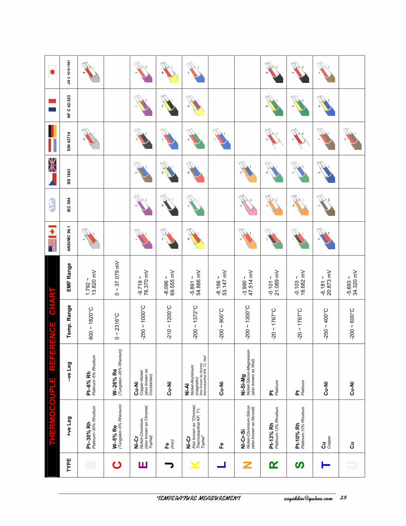
TYPE

C E J K L N

R S T


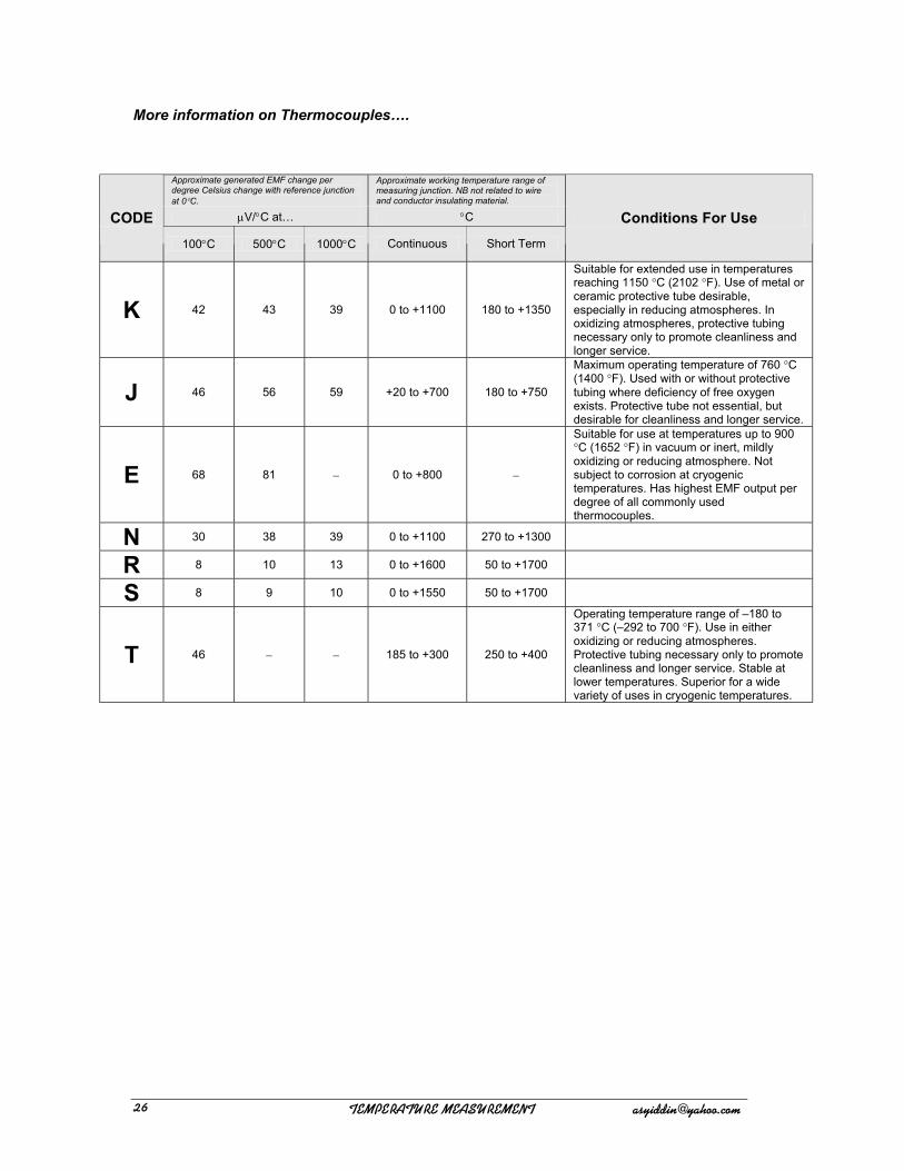
More information on Thermocouples….

Approximate generated EMF change per degree Celsius change with reference junction at 0°C.

Approximate working temperature range of measuring junction. NB not related to wire and conductor insulating material.

µV/°C at… °C CODE 100°C 500°C 1000°C Continuous Short Term

Conditions For Use

K 42 43 39 0 to +1100 180 to +1350

Suitable for extended use in temperatures reaching 1150 °C (2102 °F). Use of metal or ceramic protective tube desirable, especially in reducing atmospheres. In oxidizing atmospheres, protective tubing necessary only to promote cleanliness and longer service.

J 46 56 59 +20 to +700 180 to +750

Maximum operating temperature of 760 °C (1400 °F). Used with or without protective tubing where deficiency of free oxygen exists. Protective tube not essential, but desirable for cleanliness and longer service.

E 68 81 − 0 to +800 −

Suitable for use at temperatures up to 900 °C (1652 °F) in vacuum or inert, mildly oxidizing or reducing atmosphere. Not subject to corrosion at cryogenic temperatures. Has highest EMF output per degree of all commonly used thermocouples.

N 30 38 39 0 to +1100 270 to +1300

R 8 10 13 0 to +1600 50 to +1700

S 8 9 10 0 to +1550 50 to +1700

T 46 − − 185 to +300 250 to +400

Operating temperature range of –180 to 371 °C (–292 to 700 °F). Use in either oxidizing or reducing atmospheres. Protective tubing necessary only to promote cleanliness and longer service. Stable at lower temperatures. Superior for a wide variety of uses in cryogenic temperatures.


Resistance Temperature Resistance thermometry utilises the characteristics relationship of electrical resistance with temperature to measure temperature, generally as follow;

Rt = Ro (1 + αt) Rt = Ro (1 + αt)

where, Rt = resistance at temperature t

Ro = resistance at reference temperature (usually at ice point, 0°C) α = temperature coefficient of resistance For pure metals, this relationship can be expressed as; Rt = Ro (1 + at + bt² + ct³ + ……. )

where, Rt = resistance at temperature t Ro = resistance at reference temperature (usually at ice point, 0°C)

a = temperature coefficient of resistance b, c = coefficient calculated on the basis of two or more known resistance-temperature (calibrated) points

Significant temperature measurement accuracy improvement can be attained using a temperature sensor that is matched to a temperature transmitter. This matching process entails teaching the temperature transmitter the relationship between resistance and temperature for a specific RTD sensor. This relationship, approximated by the Callendar-Van Dusen equation, is described as:

Rt = Ro + Ro α[t – δ(0.01t – 1)(0.01t) – β(0.01t – 1)(0.01t3)]

Rt = Resistance (ohms) at Temperature t (°C) Ro = Sensor-specific Constant (Resistance at t = 0 °C) α = Sensor-specific Constant δ = Sensor-specific Constant β = Sensor-specific Constant (0 at t > 0 °C; 0.11 at t < 0 °C)

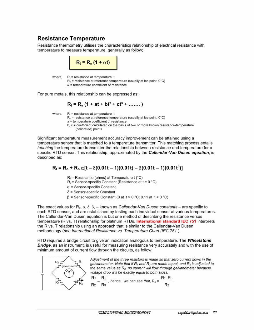
The exact values for R0, α, δ, β, – known as Callendar-Van Dusen constants – are specific to each RTD sensor, and are established by testing each individual sensor at various temperatures. The Callendar-Van Dusen equation is but one method of describing the resistance versus temperature (R vs. T) relationship for platinum RTDs. International standard IEC 751 interprets the R vs. T relationship using an approach that is similar to the Callendar-Van Dusen methodology (see International Resistance vs. Temperature Chart (IEC 751 ). RTD requires a bridge circuit to give an indication analogous to temperature. The Wheatstone Bridge, as an instrument, is useful for measuring resistance very accurately and with the use of minimum amount of current flow through the circuits, as follow;

galvanometer R1 R2

R3 RX

Adjustment of the three resistors is made so that zero current flows in the galvanometer. Note that if R1 and R2 are made equal, and Rx is adjusted to the same value as R3, no current will flow through galvanometer because voltage drop will be exactly equal to both sides.

3

x

2

1

RR

RR

= , hence, we can see that, Rx = 2

31

RRR ⋅


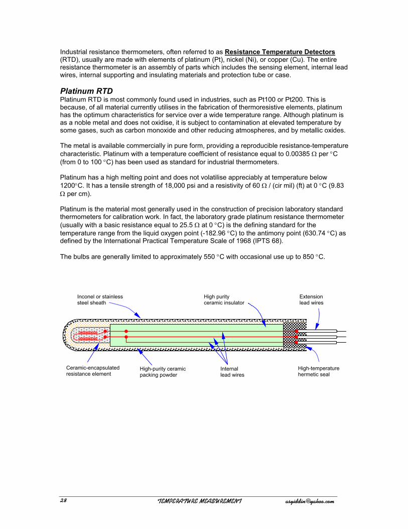
Industrial resistance thermometers, often referred to as Resistance Temperature Detectors (RTD), usually are made with elements of platinum (Pt), nickel (Ni), or copper (Cu). The entire resistance thermometer is an assembly of parts which includes the sensing element, internal lead wires, internal supporting and insulating materials and protection tube or case. Platinum RTD Platinum RTD is most commonly found used in industries, such as Pt100 or Pt200. This is because, of all material currently utilises in the fabrication of thermoresistive elements, platinum has the optimum characteristics for service over a wide temperature range. Although platinum is as a noble metal and does not oxidise, it is subject to contamination at elevated temperature by some gases, such as carbon monoxide and other reducing atmospheres, and by metallic oxides. The metal is available commercially in pure form, providing a reproducible resistance-temperature characteristic. Platinum with a temperature coefficient of resistance equal to 0.00385 Ω per °C (from 0 to 100 °C) has been used as standard for industrial thermometers. Platinum has a high melting point and does not volatilise appreciably at temperature below 1200°C. It has a tensile strength of 18,000 psi and a resistivity of 60 Ω / (cir mil) (ft) at 0 °C (9.83 Ω per cm). Platinum is the material most generally used in the construction of precision laboratory standard thermometers for calibration work. In fact, the laboratory grade platinum resistance thermometer (usually with a basic resistance equal to 25.5 Ω at 0 °C) is the defining standard for the temperature range from the liquid oxygen point (-182.96 °C) to the antimony point (630.74 °C) as defined by the International Practical Temperature Scale of 1968 (IPTS 68). The bulbs are generally limited to approximately 550 °C with occasional use up to 850 °C.

Inconel or stainless steel sheath

High purity ceramic insulator

Extension lead wires

High-temperature hermetic seal

Internal lead wires

High-purity ceramic packing powder

Ceramic-encapsulated resistance element


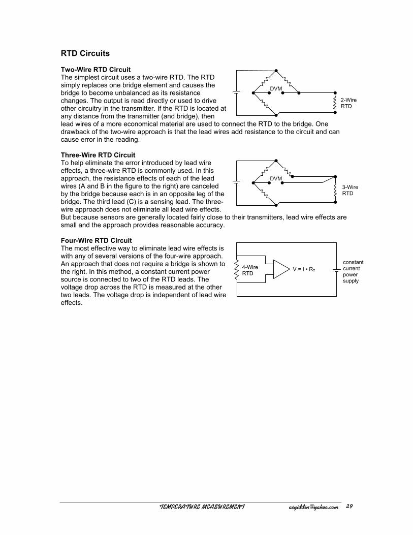
RTD Circuits Two-Wire RTD Circuit The simplest circuit uses a two-wire RTD. The RTD simply replaces one bridge element and causes the bridge to become unbalanced as its resistance changes. The output is read directly or used to drive other circuitry in the transmitter. If the RTD is located at any distance from the transmitter (and bridge), then lead wires of a more economical material are used to connect the RTD to the bridge. One drawback of the two-wire approach is that the lead wires add resistance to the circuit and can cause error in the reading.

DVM

2-Wire RTD

Three-Wire RTD Circuit To help eliminate the error introduced by lead wire effects, a three-wire RTD is commonly used. In this approach, the resistance effects of each of the lead wires (A and B in the figure to the right) are canceled by the bridge because each is in an opposite leg of the bridge. The third lead (C) is a sensing lead. The three-wire approach does not eliminate all lead wire effects. But because sensors are generally located fairly close to their transmitters, lead wire effects are small and the approach provides reasonable accuracy.

DVM 3-Wire RTD

Four-Wire RTD Circuit

V = I • RT 4-Wire RTD

The most effective way to eliminate lead wire effects is with any of several versions of the four-wire approach. An approach that does not require a bridge is shown to the right. In this method, a constant current power source is connected to two of the RTD leads. The voltage drop across the RTD is measured at the other two leads. The voltage drop is independent of lead wire effects.

constant current power supply

! !!!!!!!!!!!!!!!!!!!!!!!!!!!!!!!!!!!!!!!!!!!!!UFNQFSBUVSF!NFBTVSFNFOU!!!!!!!!!!!!!!!!!!!!!!!!btzjeejoAzbipp/dpn! 3:

SUMMARY EQUATIONS OF RTD CIRCUITS

c b a

R3

R2 R1

a

b

X

R3

R2 R1

X

Two-Lead measuring circuit R1 + R3 = R2 + a + b + X R1 = R2 R3 = a + b + X

Three-Lead measuring circuit R1 + R3 + a + c = R2 + b + c + X R1 = R2 If a = b (lead resistance equal) Then, R3 = X

C

R1 R2

X T

C C t T Ra Rb C C

X

R2 R1

Four-Lead measuring circuit

R1 + Ra + C + C = R2 + T + X + C but R1 = R2 Ra + C = T + X ----------- (1)

R1 + Rb + T + t = R2 + C + X + t but R1 = R2 Rb + C = T + X ----------- (2)

Summing equations (1) and (2), yields:

Ra + Rb + C + T = T + C + 2X

X = 2

RbRa +


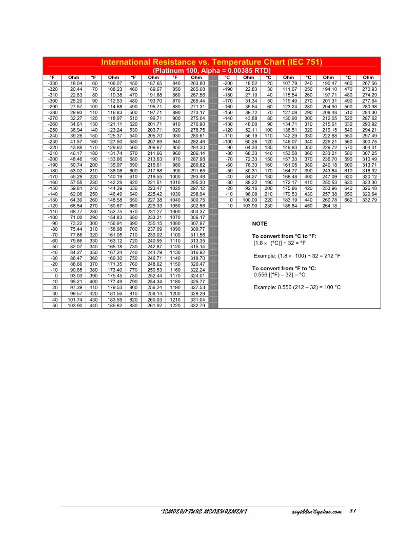
International Resistance vs. Temperature Chart (IEC 751)

(Platinum 100, Alpha = 0.00385 RTD) °F Ohm °F Ohm °F Ohm °F Ohm °C Ohm °C Ohm °C Ohm °C Ohm

-330 18.04 60 106.07 450 187.65 840 263.80 -200 18.52 20 107.79 240 190.47 460 267.56 -320 20.44 70 108.23 460 189.67 850 265.68 -190 22.83 30 111.67 250 194.10 470 270.93 -310 22.83 80 110.38 470 191.68 860 267.56 -180 27.10 40 115.54 260 197.71 480 274.29 -300 25.20 90 112.53 480 193.70 870 269.44 -170 31.34 50 119.40 270 201.31 490 277.64 -290 27.57 100 114.68 490 195.71 880 271.31 -160 35.54 60 123.24 280 204.90 500 280.98 -280 29.93 110 116.83 500 197.71 890 273.17 -150 39.72 70 127.08 290 208.48 510 284.30 -270 32.27 120 118.97 510 199.71 900 275.04 -140 43.88 80 130.90 300 212.05 520 287.62 -260 34.61 130 121.11 520 201.71 910 276.90 -130 48.00 90 134.71 310 215.61 530 290.92 -250 36.94 140 123.24 530 203.71 920 278.75 -120 52.11 100 138.51 320 219.15 540 294.21 -240 39.26 150 125.37 540 205.70 930 280.61 -110 56.19 110 142.29 330 222.68 550 297.49 -230 41.57 160 127.50 550 207.69 940 282.46 -100 60.26 120 146.07 340 226.21 560 300.75 -220 43.88 170 129.62 560 209.67 950 284.30 -90 64.30 130 149.83 350 229.72 570 304.01 -210 46.17 180 131.74 570 211.66 960 286.14 -80 68.33 140 153.58 360 233.21 580 307.25 -200 48.46 190 133.86 580 213.63 970 287.98 -70 72.33 150 157.33 370 236.70 590 310.49 -190 50.74 200 135.97 590 215.61 980 289.82 -60 76.33 160 161.05 380 240.18 600 313.71 -180 53.02 210 138.08 600 217.58 990 291.65 -50 80.31 170 164.77 390 243.64 610 316.92 -170 55.29 220 140.19 610 219.55 1000 293.48 -40 84.27 180 168.48 400 247.09 620 320.12 -160 57.55 230 142.29 620 221.51 1010 295.30 -30 88.22 190 172.17 410 250.53 630 323.30 -150 59.81 240 144.39 630 223.47 1020 297.12 -20 92.16 200 175.86 420 253.96 640 326.48 -140 62.06 250 146.49 640 225.42 1030 298.94 -10 96.09 210 179.53 430 257.38 650 329.64 -130 64.30 260 148.58 650 227.38 1040 300.75 0 100.00 220 183.19 440 260.78 660 332.79 -120 66.54 270 150.67 660 229.33 1050 302.56 10 103.90 230 186.84 450 264.18 -110 68.77 280 152.75 670 231.27 1060 304.37 -100 71.00 290 154.83 680 233.21 1070 306.17 -90 73.22 300 156.91 690 235.15 1080 307.97 -80 75.44 310 158.98 700 237.09 1090 309.77 -70 77.66 320 161.05 710 239.02 1100 311.56 -60 79.86 330 163.12 720 240.95 1110 313.35 -50 82.07 340 165.18 730 242.87 1120 315.14 -40 84.27 350 167.24 740 244.79 1130 316.92 -30 86.47 360 169.30 750 246.71 1140 318.70 -20 88.66 370 171.35 760 248.62 1150 320.47 -10 90.85 380 173.40 770 250.53 1160 322.24

0 93.03 390 175.45 780 252.44 1170 324.01 10 95.21 400 177.49 790 254.34 1180 325.77 20 97.39 410 179.53 800 256.24 1190 327.53 30 99.57 420 181.56 810 258.14 1200 329.29

NOTE To convert from °C to °F: [1.8 × (°C)] + 32 = °F Example: (1.8 × 100) + 32 = 212 °F To convert from °F to °C: 0.556 [(°F) – 32] = °C Example: 0.556 (212 – 32) = 100 °C

40 101.74 430 183.59 820 260.03 1210 331.04 50 103.90 440 185.62 830 261.92 1220 332.79


Radiation Types (Pyrometer) When temperature must be measured and physical contact with the medium to be measured is impossible or impractical, use is made of thermal radiation or optical pyrometry methods and equipment. Radiation pyrometry measures the radiant heat emitted or reflected by a hot object. Practical radiation pyrometers are sensitive to a limited wavelength band of radiant energy, although theory indicates that they should be sensitive to the entire spectrum of energy radiated by the object. The operation of thermal radiation pyrometers is based on blackbody concepts and has made possible the measurement and automatic control of temperature under conditions not feasible with other temperature sensing elements. Theory of Radiation Measurements A perfect radiating body, traditionally called a blackbody, is used as the comparative standard to measure quantitatively the energy radiated by a hot object. The thermal radiation energy and temperature relationship for a blackbody condition can be expressed as; W = kTo

4

where, W = Radiant energy emitted per unit area from the blackbody. k = Stefan-Boltzmann constant. To = absolute temperature in Kelvin.

This is the Stefan-Boltzmann law and assumes the blackbody to be radiating to a receiver which is at absolute zero.

In practical applications for thermal radiation pyrometers, the transfer of radiant thermal energy takes place at temperatures above absolute zero. Thus equation has to be modified to express the radiant energy and temperature relationship under these conditions. The new equation can be expressed as;

W = σ (T4 –To4)

Where, σ = a constant. T = absolute temperature of the blackbody. To = absolute temperature of the surroundings.

Emissivity In general a rough black surface radiates more heat than a smooth bright surface at the same temperature. This effect is called emissivity and is expressed in numbers from 1 to 0. A blackbody or perfect radiator of thermal energy has an emissivity of 1. Less perfect radiating bodies have an emissivity of less than 1. Some very thin transparent surfaces have emissivities very close to zero. Other surfaces such as plastics, rubber, and textiles have emissivities close to 1. Metals have varying emissivities depending on their surface and composition. Emissivity is important, because many types of thermal radiation pyrometers require a correction to compensate for emissivity effects.


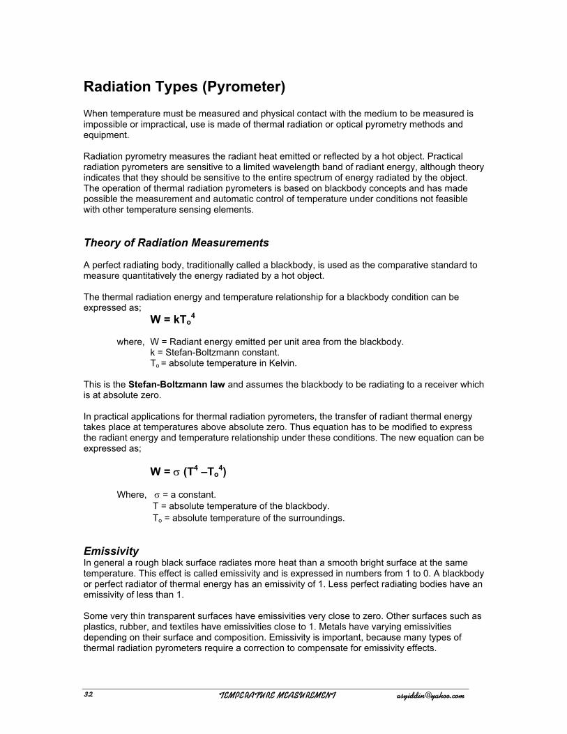
Thermal Radiation Pyrometry Thermal radiation pyrometers essentially operate according to the Stefan, Boltzmann law. This means that the pyrometer must be designed to have a wavelength response for the desired temperature range. The essential parts of a basic radiation pyrometer are shown in figure 17. The lens or mirrors used must be capable of passing or reflecting the wavelengths of the radiant energy emitted by the hot object, and focusing them of the receiving detector which gives either or emf output or undergoes a resistance change. This output can then be measured in terms of temperature by the measuring device.

Heat rays

thermopile lens

Hea

t obj

ect

measuring unit

Figure 17 : Schematic of a basic radiation pyrometer

Radiation Pyrometer Applications Radiation pyrometers are used industrially where temperatures are above the practical operating range of thermocouples, where thermocouple life is short because of corrosive atmospheres, where the object whose temperature is to be measured is moving, inside vacuum or pressure furnaces, where temperature sensors would damage the product (such as growing crystals), and for obtaining the temperature of a large surface when it is impractical to attach primary temperature sensors.


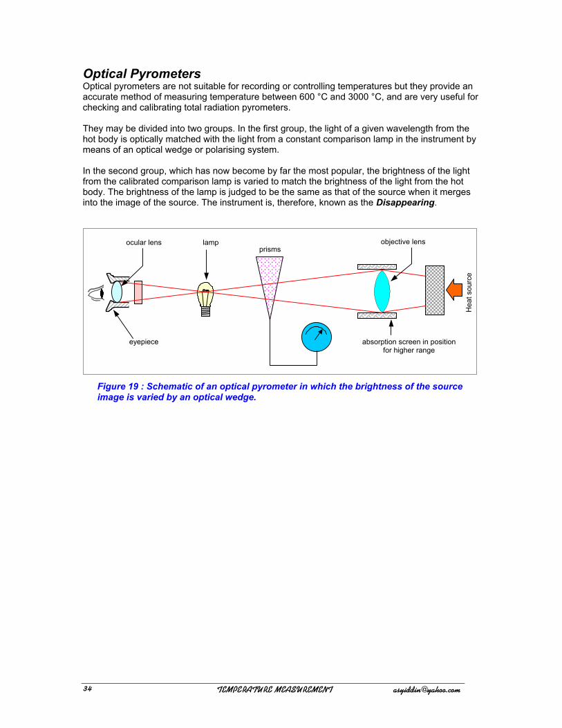
Optical Pyrometers Optical pyrometers are not suitable for recording or controlling temperatures but they provide an accurate method of measuring temperature between 600 °C and 3000 °C, and are very useful for checking and calibrating total radiation pyrometers. They may be divided into two groups. In the first group, the light of a given wavelength from the hot body is optically matched with the light from a constant comparison lamp in the instrument by means of an optical wedge or polarising system. In the second group, which has now become by far the most popular, the brightness of the light from the calibrated comparison lamp is varied to match the brightness of the light from the hot body. The brightness of the lamp is judged to be the same as that of the source when it merges into the image of the source. The instrument is, therefore, known as the Disappearing.

absorption screen in position for higher range

eyepiece

ocular lens lamp prisms

objective lens

Hea

t sou

rce

Figure 19 : Schematic of an optical pyrometer in which the brightness of the source image is varied by an optical wedge.


temperature measurement - piyush panchal home

Documents