temporal link prediction using matrix and tensor ... · temporal link prediction using matrix and...

Temporal Link Prediction using Matrix and TensorFactorizations

DANIEL M. DUNLAVY and TAMARA G. KOLDA

Sandia National Laboratories

and

EVRIM ACAR

National Research Institute of Electronics and Cryptology (TUBITAK-UEKAE)

The data in many disciplines such as social networks, web analysis, etc. is link-based, and thelink structure can be exploited for many different data mining tasks. In this paper, we consider

the problem of temporal link prediction: Given link data for times 1 through T , can we predict

the links at time T + 1? If our data has underlying periodic structure, can we predict out evenfurther in time, i.e., links at time T + 2, T + 3, etc.? In this paper, we consider bipartite graphs

that evolve over time and consider matrix- and tensor-based methods for predicting future links.

We present a weight-based method for collapsing multi-year data into a single matrix. We showhow the well-known Katz method for link prediction can be extended to bipartite graphs and,

moreover, approximated in a scalable way using a truncated singular value decomposition. Using

a CANDECOMP/PARAFAC tensor decomposition of the data, we illustrate the usefulness ofexploiting the natural three-dimensional structure of temporal link data. Through several nu-

merical experiments, we demonstrate that both matrix- and tensor-based techniques are effective

for temporal link prediction despite the inherent difficulty of the problem. Additionally, we showthat tensor-based techniques are particularly effective for temporal data with varying periodic

patterns.

Categories and Subject Descriptors: G.1.3 [Numerical Analysis]: Numerical Linear Algebra;G.1.10 [Numerical Analysis]: Applications; H.2.8 [Database Management]: Database Ap-

plications—Data mining

General Terms: Algorithms

Additional Key Words and Phrases: link mining, link prediction, evolution, tensor factorization,

CANDECOMP, PARAFAC

1. INTRODUCTION

The data in different analysis applications such as social networks, communicationnetworks, web analysis, and collaborative filtering consists of relationships, whichcan be considered as links, between objects. For instance, two people may be linkedto each other if they exchange emails or phone calls. These relationships can bemodeled as a graph, where nodes correspond to the data objects (e.g., people) andedges correspond to the links (e.g., a phone call was made between two people).The link structure of the resulting graph can be exploited to detect underlyinggroups of objects, predict missing links, rank objects, and handle many other tasks

Author Addresses: D. Dunlavy, Sandia National Laboratories, Albuquerque, NM

87123-1318, [email protected]. T. Kolda, Sandia National Laboratories, Livermore,CA 94551-9159, [email protected]. E. Acar, TUBITAK-UEKAE, Gebze, Turkey

[email protected].

Preprint submitted for publication, June 22, 2010

arX

iv:1

005.

4006

v2 [

mat

h.N

A]

19

Jun

2010

2 · D. M. Dunlavy, T. G. Kolda, and E. Acar

[Getoor and Diehl 2005].Dynamic interactions over time introduce another dimension to the challenge of

mining and predicting link structure. Here we consider the task of link predictionin time. Given link data for T time steps, can we predict the relationships at timeT + 1? This problem has been considered in a variety of contexts [Hasan et al.2006; Liben-Nowell and Kleinberg 2007; Sarkar et al. 2007]. Collaborative filteringis also a related task, where the objective is to predict interest of users to objects(movies, books, music) based on the interests of similar users [Liu and Kou 2007;Koren et al. 2009]. The temporal link prediction problem is different from missinglink prediction, which has no temporal aspect and where the goal is to predictmissing connections in order to describe a more complete picture of the overall linkstructure in the data [Clauset et al. 2008].

We extend the problem of temporal link prediction stated above to the problemof periodic temporal link prediction. For such problems, given link data for T timesteps, can we predict the relationships at times T + 1, T + 2, . . . , T + L, where Lis the length of the periodic pattern? Such problems often arise in communicationnetworks, such as e-mail and network traffic data, where weekly or monthly interac-tion patterns abound. If we can discover a temporal pattern in the data, temporalforecasting methods such as Holt-Winters [Chatfield and Yar 1988] can be used tomake predictions further out in time.

Time-evolving link data can be organized as a third-order tensor, or multi-dimensional array. In the simplest case, we can define a tensor Z of size M ×N ×Tsuch that

Z(i, j, t) =

{1 if object i links to object j at time t,

0 otherwise.

It is also possible to use weights to indicate the strength of the links. The goal is topredict the links at time T + 1 or for a period time T + 1, . . . , T + L by analyzingthe link structure of Z.

Figure 1 presents an illustration of such temporal link data for the 1991–2000DBLP bibliometric data set, which contains publication data for a large numberof professional conferences in areas related to computer science (described in moredetail in §4). The plot depicts the patterns of links between authors and conferencesover time, with blue dots denoting the links (i.e., values of 1 as defined above).

We consider both matrix- and tensor-based methods for link prediction. For thematrix-based methods, we collapse the data into a single matrix by summing (withand without weights) the matrices corresponding to the time slices. As a baseline,we consider a low-rank approximation as produced by a truncated singular valuedecomposition (TSVD). Next, we consider the Katz method [Katz 1953] (extendedto bipartite graphs), which has proven to be highly accurate in previous work onlink prediction [Huang et al. 2005; Liben-Nowell and Kleinberg 2007; Huang and Lin2009]; however, it is not always clear how to make the method scalable. Therefore,we present a novel scalable technique for computing approximate Katz scores basedon a truncated spectral decomposition (TKatz). For the tensor-based methods, weconsider the CANDECOMP/PARAFAC (CP) tensor decomposition [Carroll andChang 1970; Harshman 1970], which does not collapse the data but instead retainsits natural three-dimensional structure. Tensor factorizations are higher-order ex-

Temporal Link Prediction · 3

Fig. 1: DBLP Data for 1991–2000.

tensions of matrix factorizations that capture the underlying patterns in multi-waydata sets and have proved to be successful in diverse disciplines including chemo-metrics, neuroscience and social network analysis [Acar and Yener 2009; Kolda andBader 2009]. Moreover, CP yields a highly interpretable factorization that includesa time dimension. In terms of prediction, the matrix-based methods are limited totemporal prediction for a single time step, whereas CP can be used in solving bothsingle step and periodic temporal link prediction problems.

There are many possible applications for link prediction, such as predicting theweb pages a web surfer may visit on a given day based on past browsing history,the places that a traveler may fly to in a given month, or the patterns of computernetwork traffic. We consider two applications for link prediction. First, we con-sider computer science conference publication data with a goal of predicting whichauthors will publish at which conferences in year T + 1 given the publication datafor the previous T years. In this case, we assume we have M authors and N confer-ences. All of the methods produce scores for each (i, j) author-conference pair for atotal of MN prediction scores for year T+1. For large values of M or N , computingall possible scores is impractical due to the large memory requirements of storingall MN scores. However, we note that it is possible to easily compute subsets ofthe scores. For example, these methods can answer specific questions such as “Whois most likely to publish at the KDD conference next year?” or “Where is ChristosFaloutsos most likely to publish next year?” using only O(M +N) memory. Thisis how we envision link prediction methods being used in practice. Second, weconsider the problem of how to predict links when periodic patterns exist in thedata. For example, we consider a simulated example where data is taken daily overten weeks. We should be able to recognize, for example, weekday versus weekendpatterns and use those in making predictions. If we consider a scenario of usersaccessing various online services, we should be able to differentiate between servicesthat are heavily accessed on weekdays (e.g., corporate email) versus those that areused mostly on weekends (e.g., entertainment services).


1.1 Our Contributions

The main contributions of this paper can be summarized as follows:• Weighted methods for collapsing temporal data into a matrix are shown to out-

perform straight summation (inspired by the results in [Sharan and Neville 2008])in the case of single step temporal link prediction.

• The Katz method is extended to the case of bipartite graphs and its relationshipto the matrix SVD is derived. Additionally, using the truncated SVD, we devisea scalable method for calculating a “truncated” Katz score.

• The CP tensor decomposition is applied to temporal data. We provide bothheuristic- and forecasting-based prediction methods that use the temporal infor-mation extracted by CP.

• Matrix- and tensor-based methods are compared on DBLP bibliometric data interms of link prediction performance and relative expense.

• Tensor-based methods are applied to periodic temporal data with multiple periodpatterns. Using a forecasting-based prediction method, it is shown how themethod can be used to predict forward in time.

1.2 Notation

Scalars are denoted by lowercase letters, e.g., a. Vectors are denoted by boldfacelowercase letters, e.g., a. Matrices are denoted by boldface capital letters, e.g., A.The rth column of a matrix A is denoted by ar. Higher-order tensors are denotedby boldface Euler script letters, e.g., Z. The tth frontal slice of a tensor Z is denotedZt. The ith entry of a vector a is denoted by a(i), element (i, j) of a matrix Ais denoted by A(i, j), and element (i, j, k) of a third-order tensor Z is denoted byZ(i, j, k).

1.3 Organization

The organization of this paper is as follows. Matrix techniques are presented in §2,including a weighted method for collapsing the tensor into matrix in §2.1, the TSVDmethod in §2.2, and the Katz and TKatz methods in §2.3. The CP tensor techniqueis presented in §3. Numerical results on the DBLP data set are discussed in §4 andon simulated periodic data in §5. We discuss related work in §6. Conclusions andfuture work are discussed in §7.

2. MATRIX TECHNIQUES

We consider different matrix techniques by collapsing the matrices over time intoa single matrix. In §2.1, we present two techniques (unweighted and weighted)for combining the multi-year data into a single matrix. In §2.2, we present thetechnique of using a truncated SVD to generate link scores. In §2.3, we extend theKatz method to bipartite graphs and show how it can be computed efficiently usinga low-rank approximation.

2.1 Collapsing the data

Suppose that our data set consists of matrices Z1 through ZT of size M ×N andthe goal is to predict ZT+1. The most straightforward way to collapse that data


into a single M ×N matrix X is to sum all the entries across time, i.e.,

X(i, j) =

T∑t=1

Zt(i, j). (1)

We call this the collapsed tensor (CT) because it collapses (via a sum) the entries ofthe tensor Z along the time mode. This is similar to the approach in [Liben-Nowelland Kleinberg 2007].

We propose an alternative approach to collapsing the tensor data, motivated by[Sharan and Neville 2008], where the link structure is damped backward in timeaccording to the following formula:

X(i, j) =

T∑t=1

(1− θ)T−t Zt(i, j). (2)

The parameter θ ∈ (0, 1) can be chosen by the user or according to experimentson various training data sets. We call this the collapsed weighted tensor (CWT)because the slices in the time mode are weighted in the sum. This gives greaterweight to more recent links. See Figure 2 for a plot of f(t) = (1− θ)T−t for θ = 0.2and T = 10.

Fig. 2: Plot of the decay function f(t) = (1− θ)T−t for θ = 0.2 and T = 10.

The numerical results in §4 demonstrate improved performance using CWT ver-sus CT.

2.2 Truncated SVD

One of the methods compared in this paper is a low-rank approximation of thematrix X produced by (1) or (2). Specifically, suppose that the compact SVD ofX is given by

X = UΣVT, (3)

whereR is the rank of X, U and V are orthogonal matrices of sizesM×R andN×R,respectively, and Σ is a diagonal matrix of singular values σ1 > σ2 > · · · > σR > 0.It is well known that the best rank-K approximation of X is then given by thetruncated SVD

X ≈ UKΣKVK , (4)


where UK and VK comprise the first K columns of U and V and ΣK is the K×Kprincipal submatrix of Σ. We can write (4) as a sum of K rank-1 matrices:

X ≈K∑k=1

σkukvTk ,

where uk and vk are the kth columns of U and V respectively. The TSVD isvisualized in Figure 3.

Fig. 3: Illustration of the matrix TSVD.

A matrix of scores for predicting future links can then be calculated as

S = UKΣKVK . (5)

We call these the Truncated SVD (TSVD) scores. Low-rank approximations basedon the matrix SVD have proven to be an effective technique in many data appli-cations; latent semantic indexing [Dumais et al. 1988] is one such example. Thistechnique is called “low-rank approximation: matrix entry” in [Liben-Nowell andKleinberg 2007].

2.3 Katz

The Katz measure [Katz 1953] is arguably one of the best link predictors availablebecause it has been shown to outperform many other methods [Liben-Nowell andKleinberg 2007]. Suppose that we have an undirected graph G(V,E) on P = |V |nodes. Then the Katz score of a potential link between nodes i and j is given by

S(i, j) =

+∞∑`=1

β`|path(`)i,j |, (6)

where |path(`)i,j | is the number of paths of length ` between nodes i and j, and

β ∈ (0, 1) is a user-defined parameter controlling the extent to which longer pathsare penalized.

The Katz scores for all pairs of nodes can be expressed in matrix terms as follows.Let X be the P ×P symmetric adjacency matrix of the graph. Then the scores aregiven by

S =

+∞∑`=1

β`X`

= (I− βX)−1 − I. (7)

Here I is the P ×P identity matrix. If the graph under consideration has weightededges, X is replaced by a weighted adjacency matrix.

We address two problems with the formulation of the Katz measure. First, themethod is not scalable because it requires the inversion of a P×P matrix at a cost of


O(P 3) operations. We shall see that we can replace X by a low-rank approximationin order to compute the Katz scores more efficiently. Second, the method is onlyapplicable to square symmetric matrices representing undirected graphs. We showthat it can also be applied to our situation: a rectangular matrix representing abipartite graph.

2.3.1 Truncated Katz. Assume X has rank R ≤ P . Let the eigendecompositionof X be given by

X = WΛWT, (8)

where W is a P × P orthogonal matrix1 and Λ is a diagonal matrix with |λ1| ≥|λ2| ≥ · · · ≥ |λR| > λR+1 = · · · = λP = 0. Then the Katz scores in (7) become

S = (I− βWΛWT

)−1 − I

= W[(I− βΛ)−1 − I

]W

T= WΓW

T,

where Γ is a P × P diagonal matrix with diagonal entries

γp =1

1− βλp− 1 for p = 1, . . . , P. (9)

Observe that γp = 0 for p > R. Therefore, without loss of generality, we can assume

that W and Γ are given in compact form, i.e., Γ is just an R×R diagonal matrixand W is a P ×R orthogonal matrix.

This shows a close relationship between the Katz measure and the eigendecom-position and gives some hint as to how to incorporate a low-rank approximation.The best rank-L approximation of X is given by replacing Λ in (8) with a matrixΛL where all but the L largest magnitude diagonal entries are set to zero. Themathematics carries through as above, and the end result is that the Katz scoresbased on the rank-L approximation are

S = WLΓLWT

L

where ΓL is the L × L principal submatrix of Γ, and WL is the P × L matrixcontaining the first L columns of W.

Since it is possible to construct a rank-L approximation of the adjacency matrixin O(L|E|) operations (using an Arnoldi or Lanczos technique [Saad 1992]), thistechnique can be applied to large-scale problems at a relatively low cost. We notethat in [Liben-Nowell and Kleinberg 2007], Katz is applied to a low-rank approxi-mation of the adjacency matrix which is equivalent to what we discuss here, but itscomputation is not discussed — specifically, the fact that it can be computed effi-ciently via the formula above is not mentioned. Thus, we assume that calculationwas done directly on the dense low-rank approximation matrix given by

XL = WLΛLWT

L.

1Recall that if W is an orthogonal matrix W, then WWT = WTW = I, W−1 = WT, and

(WT)−1 = W.


We contrast this with the approach of Wang et al. [2007] who discuss an approx-imate Katz measure given by truncating the sum in (6) to the first L terms (they

recommend L = 4), i.e., S =∑4`=1 β

`X`; the main drawback of this approach is

the power matrices may be dense, depending on the connectivity of the graph.

2.3.2 Bipartite Katz & Truncated Bipartite Katz. Our problem is different thanwhat we have discussed so far because we are considering a bipartite graph, repre-sented by a weighted adjacency matrix from (1) or (2). This can be considered asa graph on P = M +N nodes where the weighted adjacency matrix is given by

X =

[0 X

XT 0

].

If X is rank R and its SVD is given as in (3), then the eigenvectors and eigenvaluesof X are given by

W =

[1√2U − 1√

2U

1√2V 1√

2V

]and Λ =

[Σ 00 −Σ

].

Note that the eigenvalues in Λ are not sorted by magnitude and the rank of X is2R. Scaling the eigenvalues in Λ as in (9), we get the 2R × 2R diagonal matrix Γwith entries

γp =

1

1− βσp− 1 for p = 1, . . . , R , and

1

1 + βσp−R− 1 for p = R+ 1, . . . , 2R.

The square matrix of Katz scores is then given by

S = WΓWT

=

[UΨ+UT UΨ−VT

VΨ−UT VΨ+VT

]where Ψ− and Ψ+ are diagonal matrices with entries

ψ−p =1

2

((1

1− βσp− 1

)−(

1

1 + βσp− 1

))=

βσp1− β2σ2

p

, and (10)

ψ+p =

1

2

((1

1− βσp− 1

)+

(1

1 + βσp− 1

))=

1

1− β2σ2p

− 1, (11)

respectively, for p = 1, . . . , R. The link scores for the bipartite graph can be ex-tracted and are given by

S = UΨ−VT. (12)

We call these the Katz scores.We can replace X by its best rank-K approximation as in (4), and the resulting

Katz scores then become

S = UKΨ−KVTK , (13)

where Ψ−K is the K ×K principal submatrix of Ψ−. We call these the TruncatedKatz (TKatz) scores. It is interesting to note that TKatz is very similar to using


TSVD except that the diagonal weights have been changed. Related methods forscaling have also been proposed in the area of information retrieval (e.g., [Bast andMajumdar 2005; Yan et al. 2008]) where exponential scaling of singular values ledto improved performance.

2.4 Computational Complexity and Memory

Computing a sparse rank-K TSVD via an Arnoldi or Lanczos method requiresO(nnz(X)) work per iteration where nnz(X) is the number of nonzeros in the ad-jacency matrix X, which is equal to the number of edges in the bipartite graph.The number of iterations is typically a small multiple of K but cannot be knownin advance. The storage of the factorization requires only K(M +N + 1) space forthe singular values and two factor matrices. Because TKatz is based on the TSVD,it requires the same amount of computation and storage for a rank-K approxima-tion. The only difference is that TKatz stores Ψ−K rather than ΣK . Katz, on theother hand, requires O(M2N +MN2 +N3) operations to compute (7) if M > N .Furthermore, it stores all of the scores explicitly, using O(MN) storage.

3. TENSOR TECHNIQUES

The data set consisting of matrices Z1 through ZT is three-way, so this lends itselfto a multi-dimensional interpretation. By analyzing this data set using a three-waymodel, we can explicitly model the time dimension and have no need to collapsethe data as discussed in §2.1.

3.1 CP Tensor Model

One of the most common and useful tensor models is CP [Carroll and Chang 1970;Harshman 1970]; see also reviews [Acar and Yener 2009; Kolda and Bader 2009].Given a three-way tensor Z of size M×N×T , its K-component CP decompositionis given by

Z ≈K∑k=1

λk ak ◦ bk ◦ ck. (14)

Here the symbol ◦ denotes the outer product2, λk ∈ R+, ak ∈ RM , bk ∈ RN , andck ∈ RT for k = 1, . . . ,K. Each summand (λk ak ◦ bk ◦ ck) is called a component,and the individual vectors are called factors. We assume ‖ak ‖ = ‖bk ‖ = ‖ ck ‖ = 1and therefore λk contains the scalar weight of the kth component. An illustrationof CP is shown in Figure 4.

The CP tensor decomposition can be considered an analogue of the SVD becauseit decomposes a tensor as a sum of rank-one tensors just as the SVD decomposes amatrix as a sum of rank-one matrices as shown in Figure 3. Nevertheless, there arealso important differences between these decompositions. The columns of U andV are orthogonal in the SVD while there is no orthogonality constraint in the CPmodel. Despite the CP model’s lack of orthogonality, Kruskal [Kruskal 1989; Koldaand Bader 2009] has shown that CP components are unique, up to permutationand scaling, under mild conditions. It is because of this property that we use CP

2A three way outer product is defined as follows: X = a ◦ b ◦ c means X(i, j, k) = a(i)b(j)c(k).


model in our studies. The uniqueness of CP enables the use of factors directly forforecasting as discussed in §3.3. On the other hand, some other tensor models suchas Tucker [Tucker 1963; 1966] suffers from rotational freedom and factors in thetime mode, thus the forecasts, can easily change depending on the rotation appliedto the factors. We leave whether or not such models would be applicable for linkprediction as a topic of future research.

Fig. 4: Illustration of the tensor CP model.

3.2 CP Scoring using a Heuristic

We make use of the components extracted by the CP model to assign scores toeach pair (i, j) according to their likelihood of linking in the future. The outerproduct of ak and bk, i.e., akb

Tk , quantifies the relationship between object pairs

in component k. The temporal profiles are captured in the vectors ck. Differentcomponents may have different trends, e.g., they may have increasing, decreasing,or steady profiles. In our heuristic approach, we assume that average activity inthe last T0 = 3 years is a good choice for the weight. We define the similarity scorefor objects i and j using a K-component CP model in (14) as the (i, j) entry of thefollowing matrix:

S =

K∑k=1

γkλkakbTk , where γk =

1

T0

T∑t=T−T0+1

ck(t). (15)

This is a simple approach, using temporal information from the last T0 = 3 timesteps only. In many cases, the simple heuristic of just averaging the last few timesteps works quite well and is sufficient. An alternative that provides a more sophis-ticated use of time is discussed in the next section.

3.3 CP Scoring using Temporal Forecasting

Alternatively, we can use the temporal profiles computed by CP as a basis forpredicting the scores in future time steps. In this work, we use the Holt-Wintersforecasting method [Chatfield and Yar 1988], which is particularly suitable for time-series data with periodic patterns. This is an automatic method which only requiresthe data and the expected period (e.g., we use L = 7 for daily data). As will beshown in §5, the Holt-Winters method is fairly accurate in picking up patterns intime and therefore can be used as a predictive tool. If we are predicting for Ltime steps in the future (one period), we get a tensor of prediction scores of size


Fig. 5: An illustration of the predictions produced by the additive Holt-Winters method on datawith a period of L = 7.

M ×N × L. This is computed as

S =

K∑k=1

λkak ◦ bk ◦ γk (16)

where each γk is a vector of length L that is the prediction for the next L timesteps from the Holt-Winters methods with ck as input.

For our studies, we implemented the additive Holt-Winters method (as describedin Chatfield and Yar [1988]), i.e., Holt’s linear trend model with additive seasonality,which corresponds to an exponential smoothing method with additive trend andadditive seasonality. For a review of exponential smoothing methods, see [Gardner2006]. An example of forecasting using additive Holt-Winters is shown in Figure 5.The input is shown in blue, and the prediction of the next L = 7 time steps isshown in red. We show examples in §5 that use the actual CP data as input.Forecasting methods beside the Holt-Winters method have also proven useful inanalyzing temporal data [Makridakis and Hibon 2000]. Work on the applicabilityof different forecasting methods for link prediction is left for future work.

3.4 Computational Complexity and Memory

The computational complexity of CP is O(nnz(Z)) per iteration. As with TSVD,we cannot predict the number of iterations in advance. The storage required forCP is K(M +N + T + 1), for the three factor matrices and the scalar λk values.

4. EXPERIMENTS WITH LINK PREDICTION FOR ONE TIME STEP

We use the DBLP data set3 to assess the performance of various link predictorsdiscussed in §2 and §3. All experiments were performed using Matlab 7.8 on a

3http://www.informatik.uni-trier.de/~ley/db/index.html


Training Test Authors Confs. Training Links Test Links Test New LinksYears Year (% Density) (% Density) (% Density)

1991-2000 2001 7108 1103 112,730 (0.14) 12,596 (0.16) 5,079 (0.06)

1992-2001 2002 8368 1211 134,538 (0.13) 16,115 (0.16) 6,893 (0.07)

1993-2002 2003 9929 1342 162,357 (0.12) 20,261 (0.15) 8,885 (0.07)

1994-2003 2004 11836 1491 196,950 (0.11) 27,398 (0.16) 12,738 (0.07)

1995-2004 2005 14487 1654 245,380 (0.10) 35,089 (0.15) 16,980 (0.07)

1996-2005 2006 17811 1806 308,054 (0.10) 40,237 (0.13) 19,379 (0.06)

1997-2006 2007 21328 1934 377,202 (0.09) 41,300 (0.10) 20,185 (0.05)

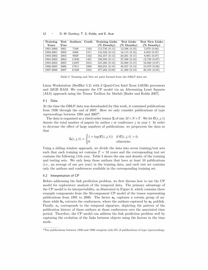
Table I: Training and Test set pairs formed from the DBLP data set.

Linux Workstation (RedHat 5.2) with 2 Quad-Core Intel Xeon 3.0GHz processorsand 32GB RAM. We compute the CP model via an Alternating Least Squares(ALS) approach using the Tensor Toolbox for Matlab [Bader and Kolda 2007].

4.1 Data

At the time the DBLP data was downloaded for this work, it contained publicationsfrom 1936 through the end of 2007. Here we only consider publications of typeinproceedings between 1991 and 20074.

The data is organized as a third-order tensor Z of size M×N×T . We let C(i, j, t)denote the total number of papers by author i at conference j in year t. In orderto decrease the effect of large numbers of publications, we preprocess the data sothat

Z(i, j, t) =

{1 + log(C(i, j, t)) if C(i, j, t) > 0,

0 otherwise.

Using a sliding window approach, we divide the data into seven training/test setssuch that each training set contains T = 10 years and the corresponding test setcontains the following 11th year. Table I shows the size and density of the trainingand testing sets. We only keep those authors that have at least 10 publications(i.e., an average of one per year) in the training data, and each test set containsonly the authors and conferences available in the corresponding training set.

4.2 Interpretation of CP

Before addressing the link prediction problem, we first discuss how to use the CPmodel for exploratory analysis of the temporal data. The primary advantage ofthe CP model is its interpretability, as illustrated in Figure 6, which contains threeexample components from the 50-component CP model of the tensor representingpublications from 1991 to 2000. The factor ak captures a certain group of au-thors while bk extracts the conferences, where the authors captured by ak publish.Finally, ck corresponds to the temporal signature, depicting the pattern of thepublication history of those authors at those conferences over the associated timeperiod. Therefore, the CP model can address the link prediction problem well bycapturing the evolution of the links between objects using the factors in the timemode.

4The publications between 1936 and 1990 comprise only 6% of publications of type inproceedings.


Figure 6a shows the third component with authors (ak) in the top plot, con-ferences (bk) in the middle, and time (ck) on the bottom. The highest scoringconferences are DAC, ICCAD and ICCD, which are related conferences on com-puter design. Many authors publish in these conferences between 1991 and 2000,but the top are Vincentelli, Brayton, and others listed in the caption. This au-thor/conference combination has a peak in the early 1990s and starts to decline inmid-’90s. Note that the author and conference scores are mostly positive. Figure 6bshows another example component, which actually has very similar conferences tothose in the component discussed above. The leading authors, however, are dif-ferent. Moreover, the time profile is different with an increasing trend after themid-’90s. Figure 7 shows a component that detects related conferences that takeplace only in even years. Again we see that the components are primarily positive.A nice feature of the CP model is that it does not have any constraints (like or-thogonality in the SVD) that artificially impose a need for negative entries in thecomponents.

4.3 Methods and Parameter Selection

The goal of a link predictor in this study is to predict whether the ith author isgoing to publish at the jth conference during the test year. Therefore, each nonzeroentry in the test set is treated as 1, i.e., a positive link, regardless of the actualnumber of publications; otherwise, it is 0 indicating that there is no link betweenthe corresponding author-conference pair.

The common parameter for all link predictors, except Katz-CT/CWT, is thenumber of components, K. In our experiments, instead of using a specific value ofK, which cannot be determined systematically, we use an ensemble approach. LetSK denote the matrix of scores computed for K = 10, 20, ...100. Then the matrixof ensemble scores, S, used for link prediction is calculated as

S =∑

K∈{10,20,...100}

SK‖SK ‖F

.

In addition to the number of components, the parameter β used in the Katz scoresin (12) and (13) needs to be determined. We use β = 0.001, which was chosensuch that ψ−p > 0 for all p = 1, . . . , R in (10) for the data in our experiments. Wehave observed that if ψ−p < 0 then the scores contain entries with large magnitudesbut negative values, which degrades the performance of Katz measure. Finally,θ is the parameter used for weighting slices while forming the CWT in (2). Weset θ = 0.2 according to preliminary tests on the training data sets. We use theheuristic scoring method discussed in §3.2 for CP.

4.4 Link Prediction Results

Two experimental set-ups are used to evaluate the performance of the methods.

Predicting All Links: The first approach compares the methods in terms of howwell they predict positive links in the test set.

Predicting New Links: The second approach addresses a more challenging prob-lem, i.e., how well the methods predict the links that have not been previouslyseen at any time in the training set.


(a) Factors from component 3: Top authors are Alberto

L. Sangiovanni Vincentelli, Robert K. Brayton, SudhakarM. Reddy, and Irith Pomeranz. Top conferences are

DAC, ICCAD, and ICCD.

(b) Factors from component 4: Top authors are MiodragPotkonjak, Massoud Pedram, Jason Cong, and AndrewB. Kahng. Top conferences are DAC, ICCAD, and AS-

PDAC.

Fig. 6: Examples from 50-component CP model of publications from 1991 to 2000.

As an evaluation metric for link prediction performance, we use the area underthe receiver operating characteristic curve (AUC) because it is viewed as a robustmeasure in the presence of imbalance [Stager et al. 2006], which is important sinceless than 0.2% of all possible links exist in our testing data. Figure 8 shows theperformance of each link predictor in terms of AUC when predicting all links (bluebars) and new links (red bars). As expected, the AUC values are much lower forthe new links. Among all methods, the best performing method in terms of AUC isKatz-CWT. Further, CWT is consistently better on average than the correspondingCT methods, which shows that giving more weight to the data in recent years


Fig. 7: Factors from component 46 of 50-component CP model of publications from 1991 to 2000:Top authors are Franz Baader, Henri Prade, Didier Dubois, and Bernhard Nebel. Top conferences

are ECAI and KR.

Fig. 8: Average link prediction performance of each method across all seven training/test set pairs

(black bars show absolute range).

improves link prediction.In Figure 9, we show the ROC (receiver operating characteristic) curves; for the

purposes of clarity, we omit the CT results. When predicting all links, Figure 9ashows that all methods perform similarly initially, but Katz-CWT is best as thefalse positive rate increases. TKatz-CWT and TSVD-CWT are only slightly worsethan Katz-CWT. Finally, CP starts having false-positives earlier than the othermethods. Figure 9b shows the behavior for just the new links. In this case, therelative performance of the algorithms is mostly unchanged.


(a) Prediction of all links in the test sets. (b) Prediction of new links in the test sets.

Fig. 9: Average ROC curves showing the performance of link prediction methods across all train-

ing/test sets.

In order to understand the behavior of different link predictors better, we alsocompute how many correct links (true positives) are in the top 1000 scores predictedby each method. Table II shows that CP, TSVD-CWT, TKatz-CWT and Katz-CWT achieve close to 75% accuracy over all links. The accuracy of the methodsgoes down to 10% or less when we remove all previously seen links from the testset, but this is still very significant. Although 10% accuracy may seem low, this isstill two orders of magnitude better than what would be expected by chance (0.1%)due to high imbalance in the data (see the last column of Table I). Note that thebest methods in terms of AUC, i.e., Katz-CT and Katz-CWT, perform worse thanCP, TSVD-CWT and TKatz-CWT for predicting new links. We also observe thatCP is among the best methods when we look at the top predictions even if it startsgiving false-positives earlier than other methods.

The matrix-based methods (TSVD, TKatz and Katz) are quite fast relative tothe CP method. Average timings across all training sets are TSVD-CT/CWT andTKatz-CT/CWT: 61 sec.; Katz-CT: 80 sec.; Katz-CWT: 74 sec.; and CP: 1300 sec.Note that for all but the Katz method, the times reflect the computation of modelsusing ranks of K = 10, 20, ...100. For the Katz method, a full SVD decompositionis computed, thus making the method too computationally expensive for very largeproblems.

5. EXPERIMENTS WITH LINK PREDICTION FOR MULTIPLE TIME STEPS

As might be evident from Figures 6 and 7, the utility of tensor models is in theirability to reveal patterns in time. In this section, we use synthesized data to explorethe ramifications of temporal predictions in situations where there are several differ-ent periodic patterns in the data. In particular, Figure 7 shows an every other yearpattern in the data, but this is not exploited in the predictions in the last sectionbased on the heuristic score in (15). In the DBLP data set, periodic time profileswere few and did not have noticeable impact on performance. Here we simulate thetype of data where bringing the time pattern information into play is crucial forpredictions. Our goal is to use the periodic information, predicting even further outin time. For example, if we assume that our training data is for times t = 1, . . . , T


Test CP TSVD TSVD TKatz TKatz Katz KatzYear -CT -CWT -CT -CWT -CT -CWT

All Links

2001 671 617 685 617 686 625 7092002 668 660 674 659 674 658 7162003 723 697 743 693 745 715 754

2004 783 726 777 721 776 719 7742005 755 716 776 720 775 700 7812006 807 729 801 731 800 698 796

2007 721 681 755 687 754 647 724

Mean 733 689 744 690 744 680 750

New Links

2001 87 80 104 80 104 51 56

2002 97 84 124 84 124 74 812003 78 80 96 75 97 55 62

2004 99 79 105 81 105 57 692005 116 89 117 88 117 58 692006 91 77 110 77 109 63 70

2007 83 71 95 73 99 43 42

Mean 93 80 107 80 107 57 64

Table II: Correct predictions in top 1000 scores.

and that the period in our data is of length L, then we can predict connections fortime periods T +1 through T +L. In this section, we present results of experimentsinvolving link prediction for multiple time steps. All experiments were performedusing Matlab 7.9 on a Linux Workstation (RedHat 5.2) with 2 Quad-Core IntelXeon 3.0GHz processors and 32GB RAM.

5.1 Data

We generate simulated data that shows connections between two sets of entities overtime. In the DBLP data, the entity sets were authors and conferences and each timet = 1, . . . , T corresponded to one year of data. In our simulated example, we assumethat each time t corresponds to one day and that the temporal profiles correspondroughly to a seven-day period (L = 7). We might assume that the entities areusers and services. For example, most major service providers (Yahoo, Google,MSN, etc.) have a front page. We may wish to predict which users will likely beconnecting to which services over time. For example, it may be that there are groupsof people that check the National, World, and Business News on weekdays; anothergroup that checks Entertainment Listings on weekends; a group that checks SportsScores on Mondays; another group uses the service for email every day, etc. Each ofthese groupings of users and services along with corresponding temporal profile canbe represented by a single component in the tensor model. The motivation for linkprediction are many-fold. We might want to characterize the temporal patterns sothat we know how often to update the services or when to schedule down time.We may use prediction to cache certain data, to better direct advertisements tousers, etc. In addition to the business model/motivation, we could also considerthe application of cybersecurity using analysis of network traffic data. In this case,the goal is to determine which computers are most likely to contact which other


Fig. 10: Example distribution of the number of nonzeros per row in entity participation matrices.

computers. Predicted links could be used to find anomalous or malicious behavior,proactively load balance, etc. In all of these applications, accurately predictinglinks over multiple time steps is crucial.

We assume that our data can be modeled by K = 10 components and generateour training and testing tensors as follows.

(1) Matrices A and B of size M×K and N×K are “entity participation” matrices.In other words, column ak (resp. bk) is the vector of participation levels of allthe entities in component k. In our tests, we use M = 500 and N = 400. Eachrow is generated by choosing between 1 and K components for the entity toparticipate in where the probability of participating in at least k+1 componentsis 1−4k. An example of the distribution of participation is shown in Figure 10;note that most entities participate in just one component. Once the number ofcomponents is decided, the specific components that a given entity participatesin are chosen uniformly at random. The strength of participation is pickeduniformly at random between 1 and 10. Finally, the columns of A and B arenormalized to length 1.

(2) In the third mode, the matrix corresponds to time. We assume we have Pperiods of training data, so that we have T = LP time observations to trainon. In our tests, we use L = 7 and P = 10. We also assume that we have 1period of testing data. Therefore, we generate a matrix C of size L(P +1)×K,

which will be divided into submatrices C[train] and C[test]. Each column of Cis temporal data of length L(P + 1) with a repeating period of length L = 7.We use the periodic patterns shown in Figure 11. For example, the first pattencorresponds to a weekday pattern, and the seventh pattern corresponds toTuesday/Thursday activities. Patterns 1 and 5 are the same but correspond todifferent sets of entities and so will still be computable in our experiments.

The creation of the temporal data is shown in Figure 12. As shown at thetop, in order to generate the temporal data of length L(P + 1), we repeat thetemporal pattern P + 1 times. Next, for each of the K = 10 components, werandomly adjust the data to be increasing, decreasing, or neutral. On the leftin the middle plot, we show a decreasing pattern and on the right an increasingpattern. Finally, we add 10% noise, as shown in the lower plots. The finalmatrix C is column normalized. The first T = LP = 70 rows become C[train]

and the last L = 7 rows become C[test].


Fig. 11: Weekly patterns of users in simulated data.

(a) Pattern 3 and a decreasing trend (b) Pattern 1 and an increasing trend

Fig. 12: Steps to creating the temporal data.

(3) We create noise-free versions of the training and testing tensors by computing

Z[train] =

K∑k=1

ak ◦ bk ◦ c[train]k and Z[test] =

K∑k=1

ak ◦ bk ◦ c[test]k .

In order to make the problem challenging, we significantly degrade the training


data in the next two steps.

(4) We take pswap = 50% of the ptop = 25% largest entries in Z[train] and randomlyswap them with other entries in the tensor selected uniformly at random. Thishas the effect of removing some important data (i.e., large entries) and alsoadding some spurious data.

(5) Finally, we add prand = 10% percent standard normal noise to every entry of

Z[train].

For each problem instance, we compute a CP decomposition of Z[train] which hashad large entries swapped and noise added. Then we use the resulting factorizationto predict the largest entries of Z[test].

5.2 Methods and Parameter Selection

The goal of this study is to predict the significant entries in Z[test]. Therefore,without loss of generality, we treat all nonzeros in the test tensor as ones (i.e.,positive links) and the rest as zeros (i.e., no link). This results in 15% positives.

We consider the CP model (with K = 10 components) using the forecastingscoring model described in §3.3. The model parameters for level, trend and sea-sonality are set to 0.2 in the Holt-Winters method. We compute the CP modelvia the CPOPT approach as described in [Acar et al. 2009]. This is an optimiza-tion approach using the nonlinear conjugate gradient method. We set the stoppingtolerance on the normalized gradient to be 10−8, the maximum number of itera-tions to 1000, and the maximum number of function values to 10,000. The modelscould have been computed using ALS as in the previous section, but here we use adifferent technique for variety.

The matrix methods described in §2 are not appropriate for this data becausesimply collapsing the data will obviously not work. Moreover, there is no clearmethodology for predicting out in time. The best we could possibly do would be toconstruct a matrix model for each day in the week (i.e., one for each ` = 1, . . . , L).Such an approach, however, is not parsimonious and would quickly become pro-hibitive as the number of models grew. Moreover, it would be extremely difficultto assimilate results across the different models for each day.

Therefore, as a comparison, we use the largest values from the most recent period.In MATLAB notation, the predictions are based on Z[train](:, :, L(P − 1) + 1 : LP ),

i.e., the last L frontal slices of Z[train]. The highest values in that period arepredicted to reappear in the testing period. We call this the Last Period method.Under the scenario considered here, this is an extremely predictive model when thenoise levels are low. As we randomly swap data (reflective of random additions anddeletions as would be expected in any real world data set), however, the performanceof this model degrades.

5.3 Interpretation of CP Results and Temporal Prediction

As mentioned above, we compute the CP factorization of a noisy version of Z[train]

of size 500× 400× 70. Because the data is noisy (swapping 50% of the 25% largestentries and adding 10% Gaussian noise), the fit of the model to the data is not


perfect. In fact, the percentage of the Z[train] that is described by the model5 isonly about 50% (averaged over 10 instances).

However, the underlying low-rank structure of the data gives us hope of recoveryeven in the presence of excessive errors. We can see this in terms of the factormatch score (FMS), which is defined as follows. Let the correct and computedfactorizations be given by

K∑k=1

λk ak ◦ bk ◦ ck and

K∑k=1

λk ak ◦ bk ◦ ck,

respectively. Without loss of generality, we assume that all the vectors have beenscaled to unit length and that the scalars are positive. Recall that there is apermutation ambiguity, so all possible matchings of components between the twosolutions must be considered. Under these conditions, the FMS is defined as

FMS = maxσ∈Π(K)

1

K

K∑k=1

(1−

|λr − λσ(k)|max{λr, λσ(k)}

)|aTk aσ(k)||bT

k bσ(k)||cTk cσ(k)|. (17)

The set Π(K) consists of all permutations of 1 to K. In our case, we just use agreedy method to determine an appropriate permutation. The FMS can be between0 and 1, and the best possible FMS is 1. For the problems mentioned above, theFMS scores are around 0.52 on average; yet the predictive power of the CP modelis very good (see §5.4).

Figure 13 shows the ten different temporal patterns in the data per the ck vectors.The green line is the original unaltered data, the first portion of which is used togenerate the training data. The blue line is the pattern that is extracted via theCP model. Note that it is generally a good fit to the true data shown in green.Finally, the red line is the prediction generated by the Holt-Winters method usingthe pattern extracted by CP (i.e., the blue line). The red data corresponds to theγk vectors used in (16) for link prediction. The results of the link prediction taskare discussed in the next subsection.

5.4 Link Prediction Results

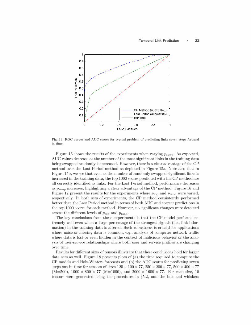
In Figure 14, we present typical ROC curves for the predictions of the next L =7 time steps (one period) for a problem instance generated using the procedurementioned above. As described in §5.2, our goal is to predict the nonzero entries inthe testing data Z[test] based on the CP model and the score in (16). We comparewith the predictions based on the last period in the data. Despite the high levelof noise, the CP method is able to get an AUC score of 0.845, which is muchbetter than then the “Last Period” method’s score of 0.686. We also consideredthe accuracy in the first 1,000 values returned. The CP-based method is 100%accurate in its top 1,000 scores whereas the “Last Period” method is only 70%accurate.

To investigate the effect of noise on the performance of the CP and Last Periodmethods, we ran several experiments varying the different amounts of noise (ptop,

5The percentage of the data described by the model is calculated as 1−‖M−Z[train]‖/‖Z[train]‖where M is the CP model.


Fig. 13: Temporal patterns using Holt-Winters forecasting. The green line is the “true” data.The blue line is the temporal pattern that is computed by CP. The red line is the pattern that ispredicted by Holt-Winters using the temporal pattern computed by CP.

pswap, and prand). For each experiments, we fixed all but one type of noise, varyingthe remaining type of noise. The fixed values for each type of noise were the sameas those for the experiment described above, while varying ptop up to 30%, pswap upto 80%, and prand up to 40%. For each level of noise, we generated 10 instances ofZ[train] and Z[test] and computed the average AUC and percentage of links correctlypredicted in the top 1000 scores.


Fig. 14: ROC curves and AUC scores for typical problem of predicting links seven steps forward

in time.

Figure 15 shows the results of the experiments when varying pswap. As expected,AUC values decrease as the number of the most significant links in the training databeing swapped randomly is increased. However, there is a clear advantage of the CPmethod over the Last Period method as depicted in Figure 15a. Note also that inFigure 15b, we see that even as the number of randomly swapped significant links isincreased in the training data, the top 1000 scores predicted with the CP method areall correctly identified as links. For the Last Period method, performance decreasesas pswap increases, highlighting a clear advantage of the CP method. Figure 16 andFigure 17 present the results for the experiments where ptop and prand were varied,respectively. In both sets of experiments, the CP method consistently performedbetter than the Last Period method in terms of both AUC and correct predictions inthe top 1000 scores for each method. However, no significant changes were detectedacross the different levels of ptop and prand.

The key conclusions from these experiments is that the CP model performs ex-tremely well even when a large percentage of the strongest signals (i.e., link infor-mation) in the training data is altered. Such robustness is crucial for applicationswhere noise or missing data is common, e.g., analysis of computer network trafficwhere data is lost or even hidden in the context of malicious behavior or the anal-ysis of user-service relationships where both user and service profiles are changingover time.

Results for different sizes of tensors illustrate that these conclusions hold for largerdata sets as well. Figure 18 presents plots of (a) the time required to compute theCP models and Holt-Winters forecasts and (b) the AUC scores for predicting sevensteps out in time for tensors of sizes 125× 100× 77, 250× 200× 77, 500× 400× 77(M=500), 1000 × 800 × 77 (M=1000), and 2000 × 1600 × 77. For each size, 10tensors were generated using the procedures in §5.2, and the box and whiskers


(a) AUC (b) Percent Correct in Top 1000

Fig. 15: Impact of varying swapping noise (pswap) averaged over 10 runs per noise value.


Fig. 16: Impact of varying random noise (ptop) averaged over 10 runs per noise value.


Fig. 17: Impact of varying random noise (prand) averaged over 10 runs per noise value.

plots in Figure 18 present the median (red center mark of boxes), middle quartile(top and bottom box edges), and outlier (red plus marks) summary statistics acrossthe experiments. These results support the conclusions above: predictions usingthe CP model are more accurate than those computed using the last period topredict an entire period of links.


(a) Timings (b) AUC

Fig. 18: Results of computing 10 CP models and Holt-Winters forecasts for tensors of differentsizes: 125× 100× 77 (M=125); 250× 200× 77 (M=250); 500× 400× 77 (M=500); 1000× 800× 77

(M=1000); 2000 × 1600 × 77 (M=2000). Computation wall clock times in seconds are shown in

(a) and AUC scores are shown in (b).

6. RELATED WORK

Getoor and Diehl [2005] present a survey of link mining tasks, including nodeclassification, group detection, and numerous other tasks including link prediction.Sharan and Neville [2008] consider the goal of node classification for temporal-relational data, suggesting the idea of a “summary graph” of weighted snapshotsin time which we have incorporated into this work.

The seminal work of Liben-Nowell and Kleinberg [2007] examines numerousmethods for link prediction on co-authorship networks in arXiv bibliometric data.However, temporal information was unused (e.g., as in [Sharan and Neville 2008])except for splitting the data. The proportion of new links ranged from 0.1–0.5%and is thus comparable to what we see in our data (0.05–0.07%). According toLiben-Nowell and Kleinberg, Katz and its variants are among the best link predic-tors; this observation has been supported by other work as well [Huang et al. 2005;Wang et al. 2007]. We note that Wang, Satuluri and Parthasarathy [2007] use thetruncated sum approximate Katz measure discussed in §2.3 and recommend AUCas one evaluation measure for link prediction because it does not require any arbi-trary cut-off. Rattigan and Jensen [2005] contend that the link mining problem istoo difficult, in part because the proportion of actual links is very small comparedto the number of possible links; specifically, they consider co-author relationshipsin DBLP data and observe that the proportion of new links is less than 0.01%.(Although we also use DBLP data, we consider author-conference links which has0.05% or more new links.)

Another way to approach link prediction is to treat it as a straightforward classifi-cation problem by computing features for possible links and using a state-of-the-artclassification engine like support vector machines. Al Hasan et al. [2006] use thisapproach in the task of author-author link prediction. They randomly pick equalsized sets of linked and unlinked pairs of authors. They compute features such askeyword similarity, neighbor similarity, shortest path, etc. However, it would likelybe computationally intractable to use such a method for computing all possiblelinks due to the size of the problem and imbalance between linked and unlinkedpairs of authors. Clauset, Moore, and Newman [2008] predict links (or anomalies)


using Monte-Carlo sampling on all possible dendrogram models of a graph. Smolaand Kondor [2003] identify connections between link prediction methods and diffu-sion kernels on graphs but provide no numerical experiments to support this.

Modeling the time evolution of graphs has been considered, e.g., by Sakar etal. [2007] who create time-evolving co-occurrence models that map entities into anevolving latent space. Tong et al. [2008] also compute centrality measures on timeevolving bipartite graphs by aggregating adjacency matrices over time in similarapproaches to those in §2.1.

Link prediction is also related to the task of collaborative filtering. In the Netflixcontest, for example, Bell and Koren [2007] consider the “binary view of the data” asimportant as the ratings themselves. In other words, it is important to first predictwho is likely to rate what before focusing on the ratings. This was a specific taskin KDD Cup 2007 [Liu and Kou 2007]. More recent models by Koren [Koren 2009]explicitly account for changes in user preferences over time. And Xiong et al. [2010]propose a probabilistic tensor factorization to address the problem of collaborativefiltering over time.

Tensor factorizations have been previously applied in web link analysis [Koldaet al. 2005] and also in social networks for the analysis of chatroom [Acar et al.2006] and email communications [Bader et al. 2007; Sun et al. 2009]. In theseapplications tensor factorizations are used as exploratory analysis tools and do notaddress the link prediction problem.

7. CONCLUSIONS

In this paper, we explore several matrix- and tensor-based approaches to solving thelink prediction problem. We consider author-conference relationships in bibliomet-ric data and a simulation indicative of user-service relationships in an online contextas example applications, but the methods presented here also have applications inother domains such as predicting Internet traffic, flight reservations, and more. Forthe matrix methods, our results indicate that using a temporal model to combinemultiple time slices into a single training matrix is superior to simple summationof all temporal data. We also show how to extend Katz to bipartite graphs (e.g.,for analyzing relationships between two different types of nodes) and to efficientlycompute an approximation to Katz based on the truncated SVD. However, noneof the matrix-based methods fully leverages and exposes the temporal signaturesin the data. We present an alternative: the CP tensor factorizations. Temporalinformation can be incorporated into the CP tensor-based link prediction analysisto gain a perspective not available when computing using matrix-based approaches.

We have considered these methods in terms of their AUC scores and the numberof correct predictions in the top scores. In both cases, we can see that all themethods do quite well on the DBLP data set. Katz has the best AUC but is notcomputationally tractable for large-scale problems; however, the other methods arenot far behind. Moreover, TKatz-CWT is best for predicting new links in theDBLP data. Our numerical results also show that the tensor-based methods arecompetitive with the matrix-based methods in terms of link prediction performance.

The advantage of tensor-based methods is that they can better capture andexploit temporal patterns. This is illustrated in the user-service example. In this


case, we accurately predicted links several days out even though the underlyingdynamics of the process was much more complicated than in the DBLP case.

The current drawback of the tensor-based approach is that there is typically ahigher computational cost incurred, but the software for these methods is quite newand will no doubt be improved in the near future.

Acknowledgments

We would like to thank the anonymous referees who provided many insightful com-ments that helped improve this manuscript.

This work was funded by the Laboratory Directed Research & Development(LDRD) program at Sandia National Laboratories, a multiprogram laboratory op-erated by Sandia Corporation, a Lockheed Martin Company, for the United StatesDepartment of Energy’s National Nuclear Security Administration under ContractDE-AC04-94AL85000.

REFERENCES

Acar, E., Camtepe, S. A., and Yener, B. 2006. Collective sampling and analysis of high order

tensors for chatroom communications. In ISI 2006: Proceedings of the IEEE InternationalConference on Intelligence and Security Informatics. Lecture Notes in Computer Science, vol.

3975. Springer, Berlin / Heidelberg, 213–224.

Acar, E., Kolda, T. G., and Dunlavy, D. M. 2009. An optimization approach for fitting

canonical tensor decompositions. Tech. Rep. SAND2009-0857, Sandia National Laboratories,Albuquerque, New Mexico and Livermore, California. Feb. Submitted for publication.

Acar, E. and Yener, B. 2009. Unsupervised multiway data analysis: A literature survey. IEEE

Transactions on Knowledge and Data Engineering 21, 1 (Jan.), 6–20.

Bader, B. W., Berry, M. W., and Browne, M. 2007. Discussion tracking in Enron emailusing PARAFAC. In Survey of Text Mining: Clustering, Classification, and Retrieval, Second

Edition, M. W. Berry and M. Castellanos, Eds. Springer, 147–162.

Bader, B. W. and Kolda, T. G. 2007. Efficient MATLAB computations with sparse and factored

tensors. SIAM Journal on Scientific Computing 30, 1 (Dec.), 205–231.

Bast, H. and Majumdar, D. 2005. Why spectral retrieval works. In SIGIR ’05: Proceedings

of the 28th annual international ACM SIGIR conference on Research and development in

information retrieval. 11–18.

Bell, R. M. and Koren, Y. 2007. Lessons from the Netflix Prize Challenge. ACM SIGKDDExplorations Newsletter 9, 75–79.

Carroll, J. D. and Chang, J. J. 1970. Analysis of individual differences in multidimensional

scaling via an N-way generalization of “Eckart-Young” decomposition. Psychometrika 35, 283–319.

Chatfield, C. and Yar, M. 1988. Holt-winters forecasting: Some practical issues. Journal ofthe Royal Statistical Society. Series D (The Statistician) 37, 2, 129–140.

Clauset, A., Moore, C., and Newman, M. 2008. Hierarchical structure and the prediction ofmissing links in networks. Nature 453.

Dumais, S. T., Furnas, G. W., Landauer, T. K., Deerwester, S., and Harshman, R. 1988.

Using latent semantic analysis to improve access to textual information. In CHI ’88: Proceedings

of the SIGCHI Conference on Human Factors in Computing Systems. ACM Press, 281–285.

Gardner, E. S. 2006. Exponential smoothing: The state of the art - part ii. International Journalof Forecasting 22, 637–666.

Getoor, L. and Diehl, C. P. 2005. Link mining: a survey. ACM SIGKDD Explorations Newslet-

ter 7, 2, 3–12.

Harshman, R. A. 1970. Foundations of the PARAFAC procedure: Models and conditions foran “explanatory” multi-modal factor analysis. UCLA working papers in phonetics 16, 1–84.

Available at http://www.psychology.uwo.ca/faculty/harshman/wpppfac0.pdf.


Hasan, M. A., Chaoji, V., Salem, S., and Zaki, M. 2006. Link prediction using supervised

learning. In Proc. SIAM Data Mining Workshop on Link Analysis, Counterterrorism, andSecurity.

Huang, Z., Li, X., and Chen, H. 2005. Link prediction approach to collaborative filtering. InJCDL ’05: Proc. of the 5th ACM/IEEE-CS joint conference on Digital libraries. 141–142.

Huang, Z. and Lin, D. K. J. 2009. The time-series link prediction problem with applications incommunication surveillance. INFORMS Journal on Computing 21, 286–303.

Katz, L. 1953. A new status index derived from sociometric analysis. Psychometrika 18, 1

(Mar.), 39–43.

Kolda, T. G. and Bader, B. W. 2009. Tensor decompositions and applications. SIAM Re-

view 51, 3 (Sept.), 455–500.

Kolda, T. G., Bader, B. W., and Kenny, J. P. 2005. Higher-order web link analysis using

multilinear algebra. In ICDM 2005: Proceedings of the 5th IEEE International Conference on

Data Mining. IEEE Computer Society, 242–249.

Koren, Y. 2009. Collaborative filtering with temporal dynamics. In KDD ’09: Proceedings of

the 15th ACM SIGKDD international conference on Knowledge discovery and data mining.ACM, New York, NY, USA, 447–456.

Koren, Y., Bell, R., and Volinsky, C. 2009. Matrix factorization techniques for recommender

systems. IEEE Computer 42, 30–37.

Kruskal, J. B. 1989. Rank, decomposition, and uniqueness for 3-way and N -way arrays. In

Multiway Data Analysis, R. Coppi and S. Bolasco, Eds. North-Holland, Amsterdam, 7–18.

Liben-Nowell, D. and Kleinberg, J. 2007. The link-prediction problem for social networks.

Journal of the American Society for Information Science and Technology 58, 7, 1019–1031.

Liu, Y. and Kou, Z. 2007. Predicting who rated what in large-scale datasets. ACM SIGKDD

Explorations Newsletter 9, 62–65.

Makridakis, S. and Hibon, M. 2000. The m3 competition: results, conclusions and implications.

International Journal of Forecasting 16, 451–476.

Rattigan, M. J. and Jensen, D. 2005. The case for anomalous link discovery. ACM SIGKDD

Explorations Newsletter 7, 2, 41–47.

Saad, Y. 1992. Numerical Methods for Large Eigenvalue Problems. Manchester University Press.

Sarkar, P., Siddiqi, S. M., and Gordon, G. J. 2007. A latent space approach to dynamic

embedding of co-occurrence data. In AI-STATS’07: Proceedings of the Eleventh International

Conference on Artificial Intelligence and Statistics (electronic).

Sharan, U. and Neville, J. 2008. Temporal-relational classifiers for prediction in evolving

domains. In ICDM ’08: Proceedings of the 2008 Eighth IEEE International Conference onData Mining. IEEE Computer Society, 540–549.

Smola, A. and Kondor, R. 2003. Kernels and regularization on graphs. In Proceedings of theAnnual Conference on Computational Learning Theory and Kernel Workshop, B. Scholkopf

and M. Warmuth, Eds. Lecture Notes in Computer Science. Springer.

Stager, M., Lukowicz, P., and Troster, G. 2006. Dealing with class skew in context recogni-

tion. In ICDCSW’06: Proceedings of the 26th IEEE International Conference on DistributedComputing Systems Workshops. 58.

Sun, J., Papadimitriou, S., Lin, C.-Y., Cao, N., Liu, S., and Qian, W. 2009. Multivis: Content-based social network exploration through multi-way visual analysis. In SDM’09: Proceedings

of the Ninth SIAM International Conference on Data Mining. 1064–1075.

Tong, H., Papadimitriou, S., Yu, P. S., and Faloutsos, C. 2008. Proximity tracking on

time-evolving bipartite graphs. In SDM’08: Proceedings of the Eighth SIAM International

Conference on Data Mining. 704–715.

Tucker, L. R. 1963. Implications of factor analysis of three-way matrices for measurement ofchange. In Problems in Measuring Change, C. W. Harris, Ed. University of Wisconsin Press,122–137.

Tucker, L. R. 1966. Some mathematical notes on three-mode factor analysis. Psychometrika 31,

279–311.


Wang, C., Satuluri, V., and Parthasarathy, S. 2007. Local probabilistic models for link

prediction. In ICDM’07: Proc. of the Seventh IEEE Conference on Data Mining. 322–331.

Xiong, L., Chen, X., Huang, T.-K., Schneider, J., and Carbonell, J. G. 2010. Temporalcollaborative filtering with bayesian probabilistic tensor factorization.

Yan, H., Grosky, W. I., and Fotouhi, F. 2008. Augmenting the power of LSI in text retrieval:

Singular value rescaling. Data & Knowledge Engineering 65, 108–125.

temporal link prediction using matrix and tensor ... · temporal link prediction using matrix and...

Documents