1

Temporal precision in the visual pathway through the interplay of excitation and stimulus-driven suppression Daniel A. Butts1, Chong Weng2, Jianzhong Jin2, Jose-Manuel Alonso2, Liam Paninski3 1Department of Biology and Program in Neuroscience and Cognitive Science, University of Maryland, College Park, MD, USA 2Department of Biological Sciences, State University of New York College of Optometry, New York, NY, USA 3Department of Statistics and Center for Theoretical Neuroscience, Columbia University, New York, NY, USA Visual neurons can respond with extremely precise temporal patterning to visual stimuli that change on much slower time scales. Here, we investigate how the precise timing of cat thalamic spike trains – which can have timing as precise as one millisecond – is related to the stimulus, in the context of both artificial noise and natural visual stimuli. Using a nonlinear modeling framework applied to extracellular data, we demonstrate that the precise timing of thalamic spike trains can be explained by the interplay between an excitatory and a delayed suppressive input that resembles inhibition, such that neuronal responses only occur in brief windows where excitation exceeds suppression. The resulting description of thalamic computation resembles earlier models of contrast adaptation, suggesting a more general role for mechanisms of contrast adaptation in visual processing. Thus, we describe a more complex computation underlying thalamic responses to artificial and natural stimuli, which has implications for understanding how visual information is represented in the early stages of visual processing. Introduction In the context of a dynamically varying visual input, visual neurons can respond with action potentials timed precisely at millisecond resolution. Such temporal precision in the visual pathway has been observed in the retina (Berry and Meister, 1998; Passaglia and Troy, 2004; Uzzell and Chichilnisky, 2004), lateral geniculate nucleus (LGN) (Butts et al., 2007; Liu et al., 2001; Reinagel and Reid, 2000), and visual cortex (Buracas et al., 1998; Kumbhani et al., 2007). This precision is notable because in many cases the neuronal response has much finer time scales than the stimulus, which might be useful in reconstructing the stimulus in artificial and natural visual stimulus contexts (Butts et al., 2007). As a result, precision is often cited as evidence for a temporal code (Borst and Theunissen, 1999; Theunissen and Miller, 1995), which posits additional information about the stimulus represented in the fine temporal features of the spike train. At the heart of elucidating the role of precision in the neural code is understanding how the timing of visual neuron responses is related to the stimulus. The relationship between the visual stimulus and the neuronal response can be captured, at a coarse level, by predictions based on a neuron’s receptive field (Chichilnisky, 2001; Simoncelli et al., 2004). While studies at finer temporal resolution reveal large discrepancies between predictions of simple receptive field based models and observed responses in retina and LGN, this is generally attributed to spike-generating machinery of the neuron (Berry and Meister, 1998; Gaudry and Reinagel, 2007; Keat et al., 2001; Paninski, 2004), in contrast to additional computation on the visual stimulus. While more complex processing is known to occur in the LGN (Alitto and Usrey, 2008; Sincich et al., 2009; Wang et al., 2010b; Wang et al., 2007), particularly in the context of adaptation (Mante et al., 2008; Shapley and Victor, 1978), such additional processing has not been explicitly linked to the issue of temporal precision. Here, we investigate the computation underlying the precise timing of LGN neurons in response to both artificial noise stimuli and natural movies, using a new statistical framework that can identify multiple stimulus-driven elements, in addition to spike refractoriness, which drive the neuron’s response. We find that a single receptive field coupled with spike-refractoriness cannot explain the observed precision of LGN responses, and instead the precise timing of spikes is modeled parsimoniously as arising from the interplay of excitation and a delayed, stimulus-driven suppression. The coordination between this excitation and suppression allows the relatively slow time courses of stimulus-driven input to cancel each other except in brief windows where excitation exceeds suppression, resulting in the observed fast response dynamics. While not previously explored in the retina and LGN, such an

2

explanation for precision has been proposed in auditory (Wehr and Zador, 2003; Wu et al., 2008), somatosensory (Gabernet et al., 2005; Okun and Lampl, 2008; Wilent and Contreras, 2005), and visual cortices (Cardin et al., 2007). Thus, in addition to its direct relevance to understanding processing in the LGN and downstream in the cortex, this work also presents a broader framework to characterize common elements of nonlinear computation in sensory pathways. METHODS Experimental Recordings All data were recorded from the LGNs of three anaesthetised and paralysed cats (either sex), and surgical and experimental procedures were performed in accordance with United States Department of Agriculture (USDA) guidelines and were approved by the Institutional Animal Care and Use Committee at the State University of New York, State College of Optometry. As described in detail in (Weng et al., 2005), cats were initially anaesthetised with Ketamine (10 mg/kg, intramuscular) followed by thiopental sodium (20 mg/kg, intravenous, supplemented as needed during surgery; and at a continuous rate of 1–2 mg/kg/hr, intravenous, during recording). A craniotomy and duratomy were made to introduce recording electrodes into the LGN (anterior: 5.5; lateral 10.5). Animals were paralysed with Atracurium Besylate (0.6–1 mg/kg/hr, intravenous) to minimize eye movements, and artificially ventilated. LGN responses were recorded extracellularly within layer A: recorded voltage signals were conventionally amplified, filtered, and passed to a computer running the RASPUTIN software package (Plexon, Dallas, Texas, United States). For each cell, spike waveforms were identified initially during the experiment and verified carefully off-line by spike sorting analysis. Cells were eliminated from this study if they did not have at least 2 Hz mean firing rates in response to all stimulus conditions, if the maximum amplitude of their spike-triggered average (STA) in spatiotemporal white noise was not at least five times greater than the amplitude outside of the receptive field area, or if their firing rate averaged over one minute changed more than 10% in successive minutes.

Visual stimuli All stimuli were displayed on a CRT display at a resolution of 0.2° per pixel with a monitor refresh rate of 120 Hz. There are two different types of stimuli used in this study: spatially uniform noise and natural movies. The spatially uniform noise consists of a temporal sequence of luminances displayed uniformly over the entire monitor, with the luminance at each time step selected from a Gaussian distribution with “zero” mean (corresponding to the midway point of the full range of monitor luminance) and an RMS contrast of 0.55, presented at 120 Hz. A two-minute sequence is used to estimate model parameters, and then 64 repeats of a 10 sec unique stimulus sequence is used for cross-validation. The natural movie sequence was produced by members of the laboratory of Peter König (Institute of Neuroinformatics, ETH/UNI Zürich, Switzerland) using a removable lightweight CCD-camera mounted to the head of a freely roaming cat in natural environments such as grassland and forest (Kayser et al., 2004). A 48×48 windowed area was processed to play at 60 Hz and have a constant mean and standard deviation of luminance for each frame (contrast held at 0.4 of maximum), as described in (Lesica and Stanley, 2006). The natural movie experiment consists of a single 15-minute sequence, with the last 10 seconds of each 90-second interval set aside for cross-validation. Model parameters are determined using the other 800 seconds).

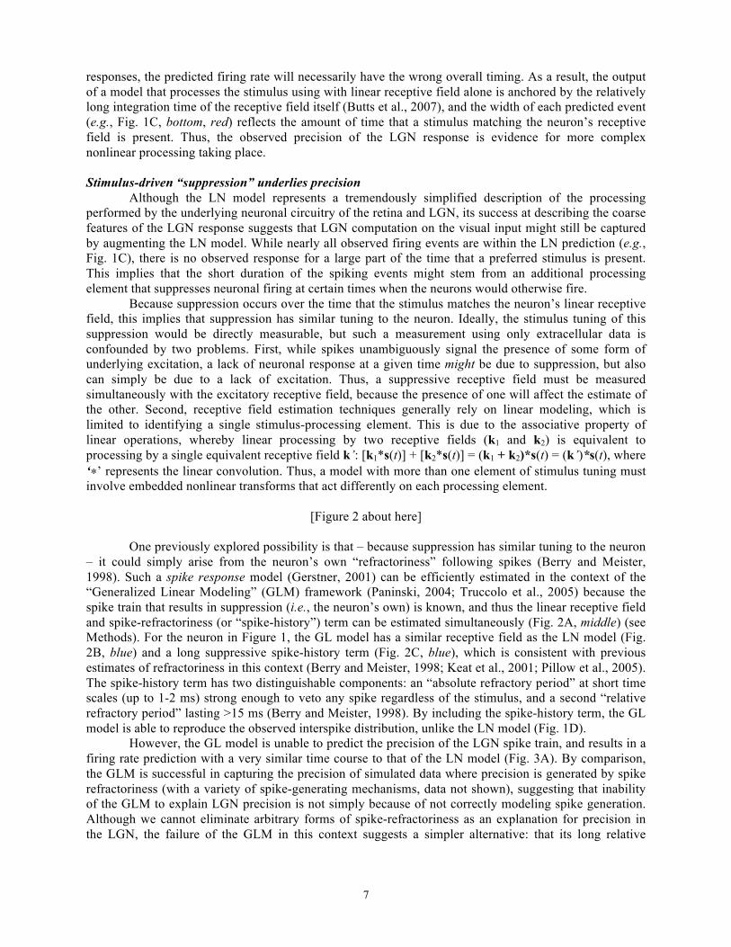
A different group of neurons was presented with the spatially uniform sequence (N = 21) versus the natural movie condition (N = 20). Care was taken to ensure that the potential effects of phase locking to the monitor refresh did not affect our results (Butts et al., 2007). Implementation of the Generalized Nonlinear Model (GNM) framework The GNM framework is an extension of the generalized linear modeling (GLM) framework described in (Brillinger, 1992; McCullagh and Nelder, 1989; Paninski, 2004; Simoncelli et al., 2004; Truccolo et al., 2005). Both models predict the instantaneous firing rate of the neuron r(t) at a given time t given the stimulus s(t), the history of observed spike train R(t), and potentially other fixed functions of the stimulus such as Wsup(t) (described below):

r(t) = F[ k * s(t) + hspk * R(t) + hsup * Wsup(t) - θ ]

(1)

Here, the parameters of the model are all linear functions inside the spiking nonlinearity F: the linear [excitatory] receptive k, the spike-history term hspk, a “postsynaptic current” (PSC) term hsup associated with Wsup, and threshold θ. Note that bold-face is used to denote multi-dimensional parameters (i.e., vectors) such that, for example k = k(τ) = [k(0) k(1) k(2) …], and ‘*’ represents temporal convolution, such that k*s(t) = ∫ k(τ) s(t-τ) dτ = k[0] s[t] + k[1] s[t-

3

1] + k[2] s[t-2] + …. The Linear-Nonlinear (LN) model consists of only the linear receptive field (eq. 1, left) and threshold, the full “GLM” considered adds the spike-history term (middle), and the GNM encompasses all terms in equation 1. Schematics of these model structures are diagramed in Figure 2A.

The spiking nonlinearity F[.] is a fixed function satisfying conditions for efficient optimization given in Paninski (2004): F[g]=log(1+eg). Thus, equation 1 describes a GLM for the parameters k, hspk, hsup (given a fixed Wsup), and its likelihood can be efficiently optimized as follows. The point-process log-likelihood per spike is given by (Paninski, 2004):

(2)

where {ts} are the observed spike times, and Nspk is the number of observed spikes. Parameter values corresponding to the linear terms can be simultaneously optimized by maximizing the likelihood of the model given the data. All model estimation uses gradient ascent of the log-likelihood, which, given the spiking nonlinearity shown above, has no local maxima other than the single global maximum (Paninski, 2004). Also, for a given choice of model parameters, both the LL and its gradient can be directly calculated, resulting in efficiently computed ascents to the globally maximum likelihood.

The GNM framework incorporates optimization of the additional parameters that comprise Wsup, which is an LN model of the stimulus s(t) with an associated receptive field ksup and internal nonlinearity fsup[.]:

(3)

For a fixed receptive field and nonlinearity, note that the output is a known function of the stimulus, and thus its associated PSC term hsup can be optimized in the context of the GLM (eq. 1). The PSC term is constrained to be negative (using a linear constraint during the optimization), making the output, hsup∗Wsup “suppressive”. Omitting this negative constraint does not improve model performance, and makes for a larger search space with more local maxima that can anchor the full parameter search (described below) to non-optimal solutions.

The suppressive nonlinearity fsup(.) can also be efficiently optimized by expressing it as a linear combination of basis functions fsup(x) = Σn αnξn[x], which are chosen to be overlapping tent-basis functions (Ahrens et al., 2008). Because the coefficients αn operate linearly on the processed stimulus ξn[ksup∗s(t)], they – and as a result a piece-wise linear approximation of fsup(.) – can also be optimized in the context of the GLM.

Thus, for a given choice of the suppressive receptive field ksup, all other terms of the GN model have a single globally optimal solution that can be found efficiently in the GLM framework. [One caveat is that the PSC term hsup and nonlinearity coefficients {αn} comprise a bilinear optimization problem requiring alternating optimization steps (Ahrens et al., 2008), which in practice converges to a global optimum.] Thus, the challenge of optimizing the GN model reduces to determining the best suppressive receptive field ksup. To limit the number of parameters used to represent ksup, we use a family of basis functions suggested in (Keat et al., 2001):

(4)

which are orthonormalized using the Gram-Schmidt method, with tF = 133 ms for the spatially uniform noise stimulus and tF = 217 ms for the natural movies. This basis set behaves like Fourier decomposition, but with the time axis scaled to have more temporal detail at short latency. With these basis functions, the observed temporal filters can be represented with relatively few terms: ten was sufficient for the spatially uniform context, and eight sufficient for the natural movies.

With the addition of model parameters inside nonlinear terms (the suppressive receptive field ksup), the relationship between model parameters and the log-likelihood becomes more complex, and no longer has a single global maximum, as with the GLM. As a result, the choice of initial guess of ksup is quite important, and we have tried several different strategies, arriving at the following. First, parameters for the GLM (including the linear receptive field and spike-history term) are estimated, and the resulting linear receptive field is then used as an initial guess for the suppressive receptive field ksup of the GNM. Optimization of ksup then proceeds by determining the LL of each choice of ksup through GLM-optimization of the PSC term and internal nonlinearities, and using this as a basis for numerical gradient ascent. We found that it is not necessary to optimize hsup and fsup(.) for each choice of ksup, but rather it is more computationally efficient to alternate between the optimization of ksup holding hsup and fsup(.) fixed, and optimization hsup and fsup(.) holding ksup fixed. We also found that this optimization is aided by constraining the internal nonlinearities to be monotonic via linear constraints, which prevented the model from

LL =1

Nspk

��

ts

log2 Pr{spk|ts}−�

t

Pr{spk|t}�

4

getting trapped in some local maxima. An example of the results of optimization of the suppressive term from the initial guess (STA) is shown in Figs. 2E-G.

Due to the estimation of model parameters at time resolutions finer than the frame rate, regularization is used to prevent over-fitting. A “smoothness” penalty term is added to the LL proportional to the squared-slope of the temporal kernels, e.g. - Σ(t) λk [k(t)-k(t+Δt)]2, with a different λ chosen for each temporal function to yield smoothly varying kernels. Note that adding penalty terms of this form to the LL still preserves the efficient properties of the GLM optimization.

After the optimal parameters are obtained, the spiking nonlinearity F[.]is re-estimated using the “histogram method” (Chichilnisky, 2001): by directly measuring the probability of a spike Pr{spk|g} for each value of the “internal” model output g (i.e., the terms in eq. (1) inside the spiking nonlinearity). The resulting estimate of Pr{spk|g} is then fit to the nonlinearity Pr{spk|g} = F[g]= α/β log[1+exp(β(g-θ)], where α is the overall slope of the non-linearity, θ is the threshold, and β determines how sharp the transition from zero firing rate is around the threshold. Empirically, the resulting estimate of F[g] described the measured spiking nonlinearity Pr{spk|g} accurately, and results in better cross-validated performance on average. Note that no saturating function was necessary.

The models applied to the spatially uniform stimulus condition were fit at a time resolution of 1/16 of the frame rate (0.5 ms), and the models in the natural movie condition were fit at a time resolution of 1/4 the frame rate (4 ms resolution). All parameter estimation was performed using Matlab (Mathworks, Natick, MA). Spatiotemporal implementation of the GNM The linear spatiotemporal receptive fields (STRFs) of retinal ganglion cells and LGN neurons are well approximated by separate center and surround components, each individually space-time separable (Allen and Freeman, 2006; Cai et al., 1997; Dawis et al., 1984). The spatiotemporal GLM firing rate can then be expressed as:

(5)

where sC(t) and sS(t) represent the spatiotemporal stimulus filtered by the “center” and “surround” spatial kernels, and kC and kS are the corresponding temporal kernels. Both spatial kernels are circular two-dimensional Gaussian distributions with the same center (x0,y0) and different widths (standard deviations) σC and σS. Because the temporal kernels and resulting model likelihood is uniquely determined by global optimization in the MLE framework, the spatial parameters can then be optimized by searching in the four-dimensional space [x0,y0,σC,σS], starting with initial values that describe the location and widths of the peak in the spike-triggered average (Butts et al., 2010). This progresses in a similar way to GNM optimization of the suppressive receptive field described above, because each combination of four spatial parameters can be uniquely associated with an optimal choice of kC and kS and an associated LL. The spatiotemporal GN model is optimized for the natural movie condition in much the same way as in the spatially uniform condition, with two main differences described below. As with the purely temporal context, the GLM STRF serves as an initial guess for the suppressive RF, and then the temporal parameters of the suppressive fields are optimized through brute force simultaneously with those of the linear “excitatory” receptive field. The first difference in the spatiotemporal case is that estimation of the additional spatial parameters, which start at values determined by the GLM. Following the first temporal optimization, the spatial parameters for linear excitatory term and suppressive term optimized simultaneously while holding the temporal parameters fixed. These temporal and spatial optimizations are alternated until there is no further improvement in the likelihood.

The second difference between the spatiotemporal model and purely temporal model is that we found that the performance of the GNM could be further improved by making the excitatory term “nonlinear” (i.e., with the same functional form as the suppressive term, eq. 3), with excitatory receptive field kexc, associated nonlinearity fexc, and PSC term hexc. After first optimizing kexc as a linear receptive field (described above), kexc was inserted as an initial guess within a nonlinear excitatory term, through alternating optimizations of kexc and ksup. The optimal values of kexc and ksup were generally very close to this initial condition. Thus, while this additional step improved model performance, it did not qualitatively change the other model parameters, other than a rectified excitatory nonlinearity that was similar to the suppressive nonlinearity (not shown).

More complex nonlinear spatiotemporal models were also tested on this dataset, and while additional complexities could yield even better model performance, the resulting fits were entirely consistent with the relationship between excitation and suppression described here (Fig. 7). As a result, a more detailed exploration of spatiotemporal processing is outside the scope of this paper.

5

The relationship between log-likelihood and information in the neuron’s spike train The log-likelihood (LL) of the data given the model (eq. 2) is directly comparable to the information that single spikes signal about the stimulus, defined as the single-spike information (Brenner et al., 2000): Iss = Σt r(t) log [r(t) / av(r)], where av(r) is the average firing rate. For example, the “null” model, whose firing rate is not modulated by the stimulus and has a constant firing rate r(t) = av(r) would have Iss = 0 , and its log-likelihood (eq. 2) given by LL0 = av(r) log av(r) - 1. Conversely, a model that perfectly predicted the firing rate would have its LL = Σt r(t) log r(t) = Iss +LL0. Because LL0 is just a constant term that depends on the number of observed spikes, maximizing the likelihood is mathematically equivalent to maximizing the information between the stimulus and the observed spike train (Kouh and Sharpee, 2009). To make this comparison explicit, we use log-base-2 in order to express the units in bits, and report the cross-validated likelihood measures with the constant LL0 subtracted (see below). Model cross-validation

Although we applied common prediction performance metrics including “percent explained variance” or R-squared (Fig. 4A,B), the main measure of model performance used in this study is the cross-validated log-likelihood (LLx), which is given by the log-likelihood of the model (eq. 2) applied to data that was not used to fit the model parameters, and with the log-likelihood of the “null model” LL0 subtracted (see the above section). This calibrates the LLx such that the null model (which just predicts the average firing rate with no stimulus modulation) has LLx = 0, and a perfect model has LLx = Iss.

Using the LLx as measure of model performance, instead of PSTH-based measures like R-squared, is particularly important because the LLx could be measured using single trials. For the spatially uniform stimulus condition, this allows the state of the neuron from trial-to-trial to be tracked. The non-stationarity that is detected as a result can be attributed to changes in the gain and offset terms (α’s and Δ respectively) applied to the parameters of the GNM:

r(t) = F{αE[k * s(t)] + αS[hsup * Wsup(t)] + αRP[hspk * Rspk(t)] – (θ – Δ) } (6)

To track these gains and additional offset over the repeated stimulus presentations, the ten-second repeated stimulus is divided into two five-second segments: the first used to fit these additional parameters using maximum likelihood estimation (while holding the standard GNM parameters constant), and the second five-second segment used for cross-validation. Regularization on the gains and offsets across successive trials is performed with an additional term added to the log-likelihood that penalized changes of the values of each gain and offset from one trial to the next. As with the smoothness penalty described above, such an additional penalty term preserves the efficiency of GLM optimization applied here (Paninski et al., 2010).

To facilitate direct comparisons across models, all reported LLx’s in this condition are measured on the same five-second segment, and incorporated optimally adjusted gains and offsets for each model. For the LN and GL models with fewer terms in equation 6, correspondingly fewer gains could be adjusted, and furthermore such adjustments had little effect on the models’ cross-validated performance. In the meantime, the spike-triggered covariance (STC) model could not be adjusted on a trial-by-trial in a straightforward manner, because its spiking nonlinearity is not parameterized and requires a large amount of data to estimate (Rahnama Rad and Paninski, 2010). In the natural movie condition, 100 sec of the 900 sec stimulus sequence that we did not fit the model to was set aside for cross-validation. The LLx reported here is thus calculated based on the likelihood of each model for this 100 sec stimulus sequence. We found that adjusting the gains and offsets in this condition did little to improve the model performance, most likely because of the much larger dimensionality of the model parameter space. The effective GN filters Because the stimulus-driven suppression of the GN model represents three stages of processing (LNL) – including two temporal convolutions – for purposes of display and comparison, we usually display an effective filter that represents the combined output of both stages. The effective filter is the cross-correlation between a Gaussian white noise stimulus (whose mean and variance match that of the true stimulus) and the output of each module driven by this noise, resulting in something akin to a spike-triggered average each for nonlinear element (e.g., eq. 3). These effective filters are pictured in Figure 3E, throughout Figure 6, and Figure 7B. Spike-triggered covariance analysis We analyzed all neurons recorded in the spatially uniform stimulus condition with the spike-triggered covariance (STC) analysis, using standard practices (Schwartz et al., 2006). Briefly, we calculated the average covariance matrix of the stimulus history preceding each spike, projecting out the spike-triggered average (STA), and then subtracted off the covariance matrix of the stimulus not triggered on spikes. The eigenvectors of this matrix

6

and the STA represent principal directions in stimulus space that best describe the distribution of spikes. For this data, they are always ‘suppressive’ (representing decreased variance), and further analysis shows that only the first suppressive STC filter consistently contributes to better cross-validated performance.

To understand the relationship between the “STC filters” (i.e., the STA and first suppressive STC eigenvector) and those found by the GNM, we measured the angles between the STC filters and the effective GN filters by normalizing each filter to have unit magnitude, and then taking the arccosine of their dot product. This also was used to project the GNM filters into the space spanned by the STC filters (Fig. 6C). The nonlinearities associated with each filter of the STC model (Fig. 6E) are calculated in the context of the GN model, and are consistent with the full two-dimensional nonlinearities associated with a full STC-based LN model. Models based on STC analysis are Linear-Nonlinear (LN) cascades, with a spiking nonlinearity F[g1,g2,…] that depends on the combined output of each linear filter, where gi(t) = s(t)*ki. The STC spiking nonlinearity can in principle be determined using the “histogram method”: just like in the one-dimensional LN model (e.g., Chichilnisky, 2001): the number of spikes in each bin (g1,g2) is normalized by the number of times each combination occurred, resulting in the probability of a spike given the pair Pr{spk|(g1, g2)}. However, the higher dimensionally of the nonlinearity stretches the number of observed spikes over many more bins, making accurate estimation methods more complicated. As a result, recently developed techniques were used for non-parametric estimation of the two-dimensional nonlinearity (Rahnama Rad and Paninski, 2010), which was used to generate a firing rate prediction.

For several neurons, maximally informative dimensions (MID) analysis (Sharpee et al., 2004) was also applied using an MID software package available online from T. Sharpee, and its results were found to be consistent with the STC analysis, as expected (Paninski, 2003; Sharpee et al., 2004). Measure of neuronal precision

To measure the amount of precision (Fig. 4D), we use the response time scale as previously defined and implemented in earlier studies (Butts et al., 2010; Butts et al., 2007; Desbordes et al., 2008). This measure is calculated from the autocorrelation of the spike train pooled across multiple repeated trials. A Gaussian distribution is fit to the central peak of the autocorrelation function, and its standard deviation σ is measured. The response time scale, corresponding to the average width of features in the PSTH of the neuron, is given by τR = σ√2 (Butts et al., 2007). RESULTS We recorded extracellularly from LGN neurons in the context of spatially uniform noise visual stimuli (Fig. 1A), a context in which spike train features are reliable to millisecond precision (Kumbhani et al., 2007; Liu et al., 2001; Reinagel and Reid, 2000). To understand the computation on the visual stimulus underlying the timing of LGN responses, we first used the familiar Linear-Nonlinear (LN) cascade model (Chichilnisky, 2001; Simoncelli et al., 2004), which is based on the neuron’s linear receptive field and typically estimated from the spike-triggered average (Chichilnisky, 2001). In the context of spatially uniform noise, the receptive field is purely temporal (because there is no spatial information in the stimulus), and the receptive field of the example LGN neuron (Fig. 1B) demonstrates both its selectivity to dark-to-light transitions (“ON cell”) and the average latency between ON transitions and the neuronal response (e.g., Fig 1A, cyan).

The LN model posits that the neuron’s firing rate simply reflects the degree that the stimulus s(t) matches the receptive field k. The firing rate prediction of the LN model is generated by making this comparison explicit with a linear convolution, resulting in the filtered stimulus g(t) (Fig. 1C, top), which is then processed by the measured spiking nonlinearity (Fig. 2D, red) that maps g(t) to a firing rate (Fig. 1C, bottom).

[Figure 1 about here]

While the LN model prediction captures the coarse timing and overall magnitude (i.e., area under firing rate curve) of the observed firing rate, it clearly does not capture the fine temporal features of the response: neither the duration of individual events, nor their precise timing (Fig. 1C, bottom). Note that this cannot be repaired by artificially constraining the spiking nonlinearity to be steeper (or even incorporating a deterministic threshold), because while this can result in more precise predicted

7

responses, the predicted firing rate will necessarily have the wrong overall timing. As a result, the output of a model that processes the stimulus using with linear receptive field alone is anchored by the relatively long integration time of the receptive field itself (Butts et al., 2007), and the width of each predicted event (e.g., Fig. 1C, bottom, red) reflects the amount of time that a stimulus matching the neuron’s receptive field is present. Thus, the observed precision of the LGN response is evidence for more complex nonlinear processing taking place.

Stimulus-driven “suppression” underlies precision

Although the LN model represents a tremendously simplified description of the processing performed by the underlying neuronal circuitry of the retina and LGN, its success at describing the coarse features of the LGN response suggests that LGN computation on the visual input might still be captured by augmenting the LN model. While nearly all observed firing events are within the LN prediction (e.g., Fig. 1C), there is no observed response for a large part of the time that a preferred stimulus is present. This implies that the short duration of the spiking events might stem from an additional processing element that suppresses neuronal firing at certain times when the neurons would otherwise fire.

Because suppression occurs over the time that the stimulus matches the neuron’s linear receptive field, this implies that suppression has similar tuning to the neuron. Ideally, the stimulus tuning of this suppression would be directly measurable, but such a measurement using only extracellular data is confounded by two problems. First, while spikes unambiguously signal the presence of some form of underlying excitation, a lack of neuronal response at a given time might be due to suppression, but also can simply be due to a lack of excitation. Thus, a suppressive receptive field must be measured simultaneously with the excitatory receptive field, because the presence of one will affect the estimate of the other. Second, receptive field estimation techniques generally rely on linear modeling, which is limited to identifying a single stimulus-processing element. This is due to the associative property of linear operations, whereby linear processing by two receptive fields (k1 and k2) is equivalent to processing by a single equivalent receptive field k’: [k1*s(t)] + [k2*s(t)] = (k1 + k2)*s(t) = (k’)*s(t), where ‘∗’ represents the linear convolution. Thus, a model with more than one element of stimulus tuning must involve embedded nonlinear transforms that act differently on each processing element.

[Figure 2 about here]

One previously explored possibility is that – because suppression has similar tuning to the neuron – it could simply arise from the neuron’s own “refractoriness” following spikes (Berry and Meister, 1998). Such a spike response model (Gerstner, 2001) can be efficiently estimated in the context of the “Generalized Linear Modeling” (GLM) framework (Paninski, 2004; Truccolo et al., 2005) because the spike train that results in suppression (i.e., the neuron’s own) is known, and thus the linear receptive field and spike-refractoriness (or “spike-history”) term can be estimated simultaneously (Fig. 2A, middle) (see Methods). For the neuron in Figure 1, the GL model has a similar receptive field as the LN model (Fig. 2B, blue) and a long suppressive spike-history term (Fig. 2C, blue), which is consistent with previous estimates of refractoriness in this context (Berry and Meister, 1998; Keat et al., 2001; Pillow et al., 2005). The spike-history term has two distinguishable components: an “absolute refractory period” at short time scales (up to 1-2 ms) strong enough to veto any spike regardless of the stimulus, and a second “relative refractory period” lasting >15 ms (Berry and Meister, 1998). By including the spike-history term, the GL model is able to reproduce the observed interspike distribution, unlike the LN model (Fig. 1D).

However, the GL model is unable to predict the precision of the LGN spike train, and results in a firing rate prediction with a very similar time course to that of the LN model (Fig. 3A). By comparison, the GLM is successful in capturing the precision of simulated data where precision is generated by spike refractoriness (with a variety of spike-generating mechanisms, data not shown), suggesting that inability of the GLM to explain LGN precision is not simply because of not correctly modeling spike generation. Although we cannot eliminate arbitrary forms of spike-refractoriness as an explanation for precision in the LGN, the failure of the GLM in this context suggests a simpler alternative: that its long relative

8

refractory period (Fig. 2C) results from this suppression being correlated with – rather than caused by – the LGN spikes. Therefore, we developed a new modeling approach to investigate a more general case where suppression is not completely explained by feedback from the neuron’s own spike train. In such a situation, the suppression can be thought to have its own stimulus tuning, represented by a “suppressive receptive field” ksup. As previously mentioned, a second receptive field alone would not be distinguishable from the original “excitatory” receptive field without some associated nonlinearity. Furthermore, for the output of filtering by the suppressive receptive field to be only suppressive (i.e., negative), it must be [nonlinearly] processed such that it only has a negative output. Thus, we model this suppression with a three-stage cascade: a linear receptive field ksup, followed by a static nonlinear function fsup, and then followed by a negatively constrained temporal filter hsup that determines how it influences the neuron’s output (Fig. 2A, right). This LNL cascade structure (Korenberg et al., 1989) gives the model flexibility to capture the effects of an inhibitory input, which could be thought of as an LN-model (ksup and fsup) filtered by an “inhibitory” (negative) postsynaptic current (PSC) hsup – but the results shown below do not depend on the accuracy of this interpretation. In either case, this model can be thought of as a next-order expansion from the LN model, similar in spirit to other nonlinear approaches such as spike-triggered covariance analysis (below). However, rather than the next-order term being based on a mathematical expansion, here the next order term is specifically designed to resemble the type of suppression caused by an inhibitory synaptic input.

To determine the parameters of this model, we developed a Generalized Nonlinear Modeling (GNM) framework based on maximum likelihood estimation, which leverages many of the efficiencies of past GLM approaches (Brillinger, 1992; Paninski, 2004; Paninski et al., 2007; Pillow et al., 2008). This framework allows for the simultaneous estimation of the linear “excitatory” receptive field (Fig. 2B), spike-history term (Fig. 2C), and components of the suppressive nonlinear term (Fig. 2E-G). When applied to the same data as the previously considered models, both the linear “excitatory” and suppressive receptive fields are different than those of the linear models (Fig. 2B, E). Instead, the suppressive receptive field ends up resembling the linear “excitatory” term of the GNM (Fig. 2E compared to Fig. 2B, green), which is also similarly different than those of the linear models. The suppressive output, however, is delayed by the PSC term hsup (Fig. 2F), which has nearly the same time course as the relative refractory period section of the previously measured spike-history term (Fig. 2C). With the suppressive term now included in the model, the spike-history term now almost completely lacks suppression for intervals greater than 5 ms. Because the spike-history and PSC are fit simultaneously in the GNM (see Methods), the attenuation of the spike-history term and corresponding appearance of the suppressive PSC reflects the best description of the data, rather than any bias in the modeling framework.

Because the GN excitatory receptive field is notably slower and less biphasic than those of the LN and GL models (Fig. 2B), this suggests that the standard stimulus tuning of the neuron represented by the linear receptive field results from a combination of a slower less-biphasic excitatory tuning and the delayed suppression. Thus, this analysis reveals a different view of the stimulus-selectivity of the neuron.

[Figure 3 about here] Precision is explained by the interplay of excitatory and suppressive receptive fields The GN model is able to capture the precise timing of the LGN neuron (Fig. 3A): both the duration of individual firing events (Fig. 3B) and their precise onset times (Fig. 3C). The improved performance of the GN model is also reflected in conventional measures of model performance, such as the fraction of explained variance, or R-squared (R2) (Fig. 4A-B), and the cross-validated log-likelihood (Fig. 4C-D). For the neuron shown, the GNM explains more than double the variance of the data compared with the LN and GL models (Fig. 4B). This improved cross-validated performance of the model is particularly significant given the increased number of parameters of the GN model, which implicitly lead to worse cross-validation unless they are capturing real elements of stimulus processing. The precise timing of the model is generated by the interplay of the two receptive fields (Fig. 3D), with the output of the excitatory receptive field preceding that of the suppressive output. To picture

9

how the precise firing of the model arises from the interplay of excitation and suppression, the output of the suppressive element is inverted and shifted by the spiking threshold, such that a non-zero firing rate occurs when the amount of excitation exceeds the amount of suppression. This comparison demonstrates that the neuron’s response occurs in brief temporal windows where excitation exceeds suppression, allowing for precise response timing to emerge from relatively slow integration and processing of the stimulus (i.e., the vertical lines demarcate only a fraction of the features of the more-slowly evolving excitatory and suppressive terms). This delay is evident comparing the excitatory filter with the effective suppressive filter (Fig. 3E), calculated by the cross-correlation between the stimulus and output of the suppressive term.

By comparison, the time courses of the LN and GL model predictions are anchored to the stimulus filtering of their single linear receptive field, which is fixed by the frequency content of the stimulus combined with the filtering properties of the temporal receptive fields (Butts et al., 2007). The resulting time course of this linear stimulus filtering is comparable to that of the “excitatory” GNM filter alone (Fig. 3D, magenta), although it is shifted earlier in time such that the output peaks with the data, resulting in a latency difference in the filters themselves (Fig. 2B). While one could construct a more precise model by using a linear filter that was more high-pass, the resulting output of this filter would not describe the data, which constrains such a linear model to these slower time scales. From this perspective, the presence of the suppression in the GNM allows for the observed precision and the appropriate stimulus selectivity.

A more subtle but equally important element of the GNM processing is the suppressive nonlinearity (Fig. 2G), without which these two filters would linearly sum into a single linear filter (e.g., Fig. 2B, red). Without the nonlinear rectification of the suppressive term – the effects of which can be seen in Fig. 3D (cyan) – the suppressive term would result in excitation by the opposite stimulus type, resulting in spurious excitations that are not in the data.

The interplay of excitation and suppression as an explanation for precision is fundamentally different than the source being the dynamics of spike generation, and results in a different estimate of the underlying tuning to stimuli of the neuron (Fig. 2B). The model’s ability to predict the onset and offset times of individual firing events likely stems from the individually tuned excitatory and suppressive receptive fields, and implies the existence of a richer computation that can be accomplished in the LGN than if its responses were governed by a single receptive field – in particular for spatiotemporal stimuli (see below). Supporting this role in more general computation, the improved performance of the GN model extends to coarse time resolutions where precision is not a factor (Fig. 4A), with the GNM explaining over 80% of the variance compared with 60% of the LN model.

To demonstrate the performance gain across the population, we use the cross-validated log-likelihood LLx, which is much more sensitive than R2 and can be measured using single trials to reveal much more detail about the state of the neuron over time (see below). The LLx is in units of bits per spike, and is measured relative to the “null” model, which assumes a mean firing rate with no stimulus-tuned elements, making the LLx comparable to the model’s single-spike information (Brenner et al., 2000; Kouh and Sharpee, 2009) (see Methods). For the neuron considered above, the GN model gives a 94% improvement in the LLx, with LLx(LN) = 1.64 bits/spk and LLx(GN) = 3.18 bits/spk. Across the neurons in this study, the GN model yields an improvement over both the LN and GL models in every case (Fig. 4C), with mean 47% improvement, compared with a 15% improvement of the GL model. These results are summarized in a box plot (Fig. 4D) that compares LLx of the GN model to all other models considered in this study, including a model based on spike-triggered covariance (described below). The GN model provides a better explanation for the data for every neuron in the study, and in many cases the improved performance represents a significant proportion of the information in the spike train.

Rather than being uniform across all neurons, the improvement gained from the GN model is highest for the most precise neurons (Fig. 4E). Neurons with the strongest suppression have a narrower window over which excitation exceeds suppression, resulting in greater precision. In fact, the example neuron considered above is the most precise neuron in the study, and correspondingly had the largest improvement in the GN framework (Fig. 4E, arrow). Choosing it as an example highlights that this

10

approach is most successful with the neurons that are the least well described by the LN model, though its qualitative features are typical of all other neurons in this study.

[Figure 4 about here] Dynamic adaptation of precise timing

Although the overall performance of the GNM is significantly better on average than other models, this is often not the case for the first few trials of the repeated cross-validation stimulus (Fig. 5A). For the first few stimulus repeats, the performance of the GNM is below that of the LN and GL models, before stabilizing at a much better performance for the duration of the repeats. Because, blocks of repeated stimulus presentations used for cross-validation always followed pauses in the experiments when no visual stimulus was presented, we hypothesized that this shift might be due to adaptation in the state of the neuron during the few trials. However, the fact that this non-stationarity is not evident in the performance of the less-precise models suggests that this adaptation primarily affects the timing of the response, rather than gross changes in firing rate.

To investigate this, we allow the gains of each model component and the overall spike threshold to dynamically change from trial to trial. We fit these extra parameters using the first five seconds of each trial, and perform cross-validation using the second five seconds (see Methods). This reveals a consistent pattern across most of the population of LGN neurons in this study (N = 16 of 21): the gains of the excitation and suppression are significantly smaller initially, and quickly recover to their equilibrium values (Fig. 5B, top). At the same time, the spike threshold is initially much lower, and increases with the same time course (Fig. 5B, bottom). The result of these opposing shifts is a fairly constant firing rate, where initially lower gains are paired with a higher “offset” such that it takes less excitation to get to threshold. These trial-to-trial adjustments of the gains and offset lead to a much more consistent cross-validated performance for the initial trials (Fig. 5C), and also stabilize slower fluctuations in the LLx observed in some recordings (not shown).

Although these simultaneous adjustments of gain and threshold have only small effect on the overall firing rate, they have significant effects on the predicted timing of firing events. This is demonstrated by comparing the predicted firing rates from the first few trials versus at equilibrium (Fig. 5D). While the observed PSTH cannot be directly compared (because it takes many repeated trials to estimate), the observed spike times themselves confirm this timing relationship (Fig. 5D, top).

Thus, this trial-based analysis underscores the ability of the GNM to predict the precise timing of the neuronal spike train. Such subtle differences in timing were not detectable using previous models, and furthermore cannot be observed in the PSTH, which must be estimated from many repeated trials. Both the excitatory and suppressive gains, as well as the relative change in spiking threshold are in principle observable experimentally, and thus these modeling results make specific predictions about the effects of adaptation on response timing, as well as their underlying mechanisms.

[Figure 5 about here]

The relationship of the GNM to more general nonlinear characterizations

In explicitly modeling the nonlinear processing in LGN neurons as the sum of separate excitatory and suppressive elements, the GNM assumes a much more specific structure for the nonlinear processing of LGN neurons, compared with other nonlinear modeling approaches, such as spike-triggered covariance (STC) (de Ruyter van Steveninck and Bialek, 1988; Schwartz et al., 2006) and maximally informative dimensions (MID) (Sharpee et al., 2004). Such approaches have been recently applied to both retinal ganglion cells (RGCs) and LGN neurons (Fairhall et al., 2006; Sincich et al., 2009), but they did not find the same relationship between the multiple temporal filters. To understand the differences between solutions detected by these different methods, as well as to provide a larger context to interpret models found through nonlinear analysis, here we compare the GNM to models based on STC.

Spike-triggered covariance (STC) analysis is a widely applied nonlinear approach that can identify multiple “directions in stimulus space” that a neuron is sensitive to (de Ruyter van Steveninck

11

and Bialek, 1988; Schwartz et al., 2006). Furthermore, given the [Gaussian noise] stimulus used in this study, STC and MID solutions should theoretically obtain the same estimates given the model form (Paninski, 2003; Sharpee et al., 2004), and this was verified for several neurons (data not shown). When applied to the example neuron considered in previous figures, STC analysis reveals two relevant directions in stimulus space for most LGN neurons in this study (Fig. 6A, top): an “excitatory” STA filter, and a “suppressive” filter corresponding to the most significant dimension identified by STC. Together, these will be referred to as the STC filters. These two filters have a qualitatively similar relationship as the excitatory and suppressive receptive fields of the GNM, with suppression delayed relative to excitation. However, they are clearly quite different in detail (Fig. 6A, bottom), with the STC filters at more spread latencies and significantly more biphasic, relative to the GN filters.

The discrepancies between the temporal filters found by these different methods can be understood by considering the “subspace” of stimuli spanned by the two STC filters (Pillow and Simoncelli, 2006; Schwartz et al., 2006). The two effective GN filters are largely contained in this “STC subspace”, and thus can be represented as linear combinations of the two STC filters (Fig. 6B), with only small differences with regard to their rebound. This relationship can be pictured geometrically, by projecting all four filters into the plane defined by the STC filters (Fig. 6C), This shows that the effective GNM filters are in between the STA and suppressive STC filter, having more intermediate latencies and more closely resembling each other. Similar relationships between the STC and GN models are found with every neuron in this study, although in some cases the GNM filters did not project quite as well into the plane defined by STC (data not shown).

The different descriptions of the stimulus selectivity of these methods can be understood by picturing the locations of the stimuli associated with each spike projected into the subspace described (Fig. 6D). If the particular stimulus directions of this subspace had no relationship to the neuron’s spikes, then the spike cloud projected into this subspace would have a width (i.e., standard deviation) shown by the black circle. However, the “spike cloud” does not follow this circle, and is extended along the horizontal axis, and compressed along the vertical axis. Because the STA does indeed point to the center of the spike cloud (by definition), the decreased variance along the vertical axis is explained by a symmetric nonlinear suppression (Fig. 6E, right), which is found when mapping the spiking nonlinearity associated with this dimension (see Methods). Such symmetric suppression is common in models of contrast adaptation (Mante et al., 2008; Schwartz et al., 2006; Schwartz and Simoncelli, 2001; Shapley and Victor, 1978), where neuronal processing is based on the STA and adaptation to contrast augments this processing. The bowl-like shape of the associated nonlinearity shows that stimuli that either match or are opposite to the suppressive STC filter will cause suppression, which is often described as divisive normalization (Schwartz and Simoncelli, 2001).

[Figure 6 about here]

In contrast, the GN model suggests that the STA represents the combined effects of excitation and

suppression, and that the true excitation of the neuron points one side of the spike cloud (Fig. 6D, blue). Because of asymmetric suppression that is rectifying (not “squaring” or symmetric), only spikes on one side of the excitatory filter are suppressed (Fig. 6D, green), resulting in the same overall location of spikes along the horizontal axis. The GN and STC models thus offer different explanations for processing of excitation and suppression within the same “stimulus subspace” in a way that produces the same spike cloud (Fig. 6F).

However, as mentioned above, these descriptions are not equivalent in their ability to describe the data, and the cross-validated performance of the GN model is significantly higher compared with models based on STC for every neuron in this study (Fig. 4D). Furthermore, the GN model structure is more readily interpreted in physiological terms – potentially as separate excitatory and inhibitory processing see Discussion) – in part because of the monotonic nonlinearity (Fig. 2G) and PSC term (Fig. 2F) associated with the suppressive filter. In fact, monotonicity of the nonlinearity and non-positivity of the PSC term is explicitly enforced in the model parameter search, which speeds the fitting procedure and eliminates local maxima in the likelihood. Not doing so can often result in the GNM finding a solution

12

much more similar to the STC filters, but this occurs at a local maximum of the likelihood, rather than a global maximum. The structure of the GNM also allows for the incorporation of spike-refractoriness (Fig. 2C), which can only be taken into account in the STC model as additional filter acting on the stimulus (data not shown). In this sense, the GN model is structured to account for a biologically implementable solution, which improves model predictions, and leads to specific physiological predictions of the origins of each model component (see Discussion). Excitation and suppression generate precision in spatiotemporal contexts The time scales of LGN responses become significantly longer in the context of natural visual stimuli, but LGN responses to natural movies are still significantly more precise than would be expected by linear processing alone (Butts et al., 2010; Butts et al., 2007). To investigate whether this precision could arise from a similar interplay of excitatory and suppressive elements, we developed a spatiotemporal version of the GNM described by replacing the purely temporal receptive fields with spatiotemporal receptive fields (STRFs). Spatial processing was performed by the common Difference-of-Gaussians (DoG) model (Cai et al., 1997), consisting of overlapping “center” and “surround” circular Gaussians, each with an associated temporal kernel (e.g., Fig. 7A). This incorporates the observation that spatiotemporal processing is not space-time separable in LGN neurons, although, when considered separately, the center and surrounds themselves are (Allen and Freeman, 2006; Cai et al., 1997; Dawis et al., 1984). As with the GL and GN models described for purely temporal data, all parameters of each STRF, including the position and width of each Gaussian and their associated temporal kernels, are optimized through maximum likelihood estimation (see Methods). Note that we expect nonlinear spatiotemporal processing in LGN neurons to be more complicated than this basic phenomenological model (see for example Mante et al., 2008), but are simply aiming here for the next-order model above linear that is consistent with previous studies of spatiotemporal processing.

GL and GN models were applied to LGN recordings in the context of natural movies, recorded from a camera on the head of a cat walking in a forest (Kayser et al., 2004). Unlike spike-triggered average approaches (Theunissen et al., 2001), maximum likelihood estimation automatically adjusts for stimulus correlations, making parameter estimation in the context of natural stimuli no more difficult than with uncorrelated “noise” stimuli.

The spatiotemporal GNM in the context of natural movies results in a very similar picture of the generation of precision as compared with the spatially uniform cases considered above. For all neurons (N = 20), there was a strong suppressive term with very similar spatiotemporal properties as the excitation (Fig. 7A), although delayed through the PSC term. Note that the delay between excitation and suppression is in addition to the differences in temporal processing between center and surround of each (Fig. 7B). The spatiotemporal tuning of excitation was also significantly different than that found in the context of the LN model (using comparable maximum likelihood estimation) (Fig. 7B), which presumably combines the effects of excitation and suppression into a single linear term.

The resulting GNM predictions are a better description of the recorded spike trains than the LN model for every neuron recorded (Fig. 7C), in large part because its ability to predict the precise responses of LGN neurons (Fig. 7D). In conclusion, the interplay of excitation and suppression observed in the spatially uniform stimulus condition is also present and relevant in natural stimulus contexts, and is necessary to explain the observed precision (Butts et al., 2007), as well as more subtle features of LGN responses in these conditions that are only evident through the statistical analysis described.

13

DISCUSSION Here we provide evidence that the precise timing of LGN neuron responses reflects the interplay of excitation and stimulus-tuned suppression, which is detectable in a variety of stimulus contexts. Suppression is delayed relative to excitation, such that LGN responses occur in a brief window where the amount of excitation exceeds the amount of suppression. The interplay between these two stimulus processing elements appears to underlie the precise timing of LGN neuron responses, which has been observed both in spatially uniform noise (Kumbhani et al., 2007; Liu et al., 2001; Reinagel and Reid, 2000) and natural movies (Butts et al., 2007). Such interplay might have its origins in the retina (see below), and subsequently could also underlie the temporal precision observed in retinal ganglion cell responses (Berry and Meister, 1998; Liu et al., 2001; Passaglia and Troy, 2004; Uzzell and Chichilnisky, 2004). Likewise, such an means of generating precise neuronal responses may be quite general in sensory processing, and is similar to a proposed function of feed-forward inhibition in the somatosensory cortex (Gabernet et al., 2005; Okun and Lampl, 2008; Wilent and Contreras, 2005), auditory cortex (Wehr and Zador, 2003; Wu et al., 2008), and visual cortex (Cardin et al., 2007).

We derived this explanation of visual processing in the LGN using only extracellular [single-unit] data and statistical validation, similar in spirit (and/or methodology) to much previous work in the visual pathway (Berry and Meister, 1998; Mante et al., 2008; Pillow et al., 2008; Sincich et al., 2009; Wu et al., 2006). In this sense, observed spike times are leveraged to evaluate different hypotheses of how the visual circuit processes stimuli, and the large increase in the performance of the model proposed here over previous models of retina and LGN processing (Fig. 4D) corresponds to its ability to explain aspects of physiological data that have not been otherwise explained. Furthermore, the resemblance of the identified computation to properties of feed-forward inhibition, and the model’s success at accurately describing the precise timing of LGN spike trains, suggests new mechanistic hypotheses (see below) that might be validated by targeted intracellular experiments, as is possible in the retina (Manookin et al., 2008; Murphy and Rieke, 2006) and LGN (Wang et al., 2010b; Wang et al., 2007).

[Figure 8 about here] The possible sources of suppression The delayed suppression detected by our model most likely arises from inhibitory interneurons, with the delay due to a disynaptic pathway. Inhibitory interneurons exist in both the retina and LGN, and the effects we report may come from either or both. Most directly, interneurons in the LGN receive direct retinal input and form inhibitory synapses onto both LGN neurons and their presynaptic retinal ganglion cell terminals (Dubin and Cleland, 1977). Studies of LGN neurons in vitro found evidence for some LGN neurons that receive excitatory and inhibitory input from the same retinal ganglion cell (Blitz and Regehr, 2005), although such “Push” inhibition has not been observed in vivo (Wang et al., 2010b; Wang et al., 2007). There is also evidence that precision is at least partially generated in the retina (Berry and Meister, 1998; Murphy and Rieke, 2006; Passaglia and Troy, 2004; Uzzell and Chichilnisky, 2004) and enhanced across the retinogeniculate synapse (Carandini et al., 2007; Casti et al., 2008; Rathbun et al., 2010; Wang et al., 2010a). The LNL(N) cascade structure of the GNM (Fig. 2A) is conceptually similar to previously proposed models of retinal processing (Korenberg et al., 1989), including the effects of contrast adaptation (Meister and Berry, 1999; Shapley and Victor, 1978). This possibility is also consistent with our findings, because such retinal processing would be inherited by the LGN, and then contribute to the observed computation underlying LGN response properties.

In fact, the GNM can replicate the dominant effects of contrast adaptation, if the suppression were to be more strongly modulated by contrast than excitation (Butts and Casti, 2009; Shapley and Victor, 1981). Higher contrasts would evoke stronger suppression, and the effects of the delayed suppressive filter would impart sensitivity to higher frequencies and decreased response latency (Shapley and Victor, 1978; Zaghloul et al., 2005). Also, more suppression at high contrasts would result in lower “gain” overall. These effects can be explicitly reproduced by the GNM by decreasing the relative strength of suppression in low contrast, and can be seen in the resulting STA of simulated data (Fig. 8), yielding

14

results consistent with previous contrast studies (Chander and Chichilnisky, 2001; Zaghloul et al., 2005). While similar in structure, the GNM results suggest that “contrast normalization” may not in fact be symmetric, or sign-invariant, as in past models of adaptation (Mante et al., 2008; Meister and Berry, 1999; Schwartz and Simoncelli, 2001). Rather, the GN model finds an asymmetric solution with monotonic nonlinearities as an alternative explanation for “bowl-shaped” suppression (Fig. 6), which achieves similar computational effects, but has much better performance in reproducing the data in this study.

While contrast adaptation plays a large role in shaping the LGN response to natural movies (Mante et al., 2008), the nonlinear effects of contrast adaptation are generally not considered outside of the context of contrast-varying stimuli, except in the anticipation of moving stimuli (Berry et al., 1999). Our study thus suggests a larger role for contrast gain control mechanisms in determining the precise timing of LGN responses. In doing so, it also implies that the impact of such mechanisms can be characterized with high fidelity outside of the context of contrast adaptation. This interpretation is thus far consistent with preliminary results applying the GNM to data at multiple contrasts from cat retina (Casti et al., 2008), and would be directly verifiable through intracellular experiments in the retina, targeted to the contexts that this study suggests. Nonlinear modeling of extracellular data Rather than using intracellular recording, we measured putative excitatory and inhibitory tuning underlying LGN neuron responses using extracellular recordings (Butts et al., 2007). An internal nonlinear stage in the GNM (Fig. 4A) allows for multiple stimulus-tuned elements that contribute nonlinearly to the LGN response, and efficient maximum likelihood estimation (Paninski, 2004) can be used to find both the receptive field filters and their associated nonlinearities. This approach thus joins several other nonlinear approaches that can identify multiple receptive fields, including spike-triggered covariance (STC) (de Ruyter van Steveninck and Bialek, 1988; Pillow and Simoncelli, 2006; Schwartz et al., 2006), maximally-informative dimensions (MID) (Sharpee et al., 2004), information-theoretic spike-triggered average and covariance (iSTAC) (Pillow and Simoncelli, 2006), and neural network approaches (Lau et al., 2002; Prenger et al., 2004).

Other techniques have previously identified the presence of multiple stimulus tuned elements in the retina (Fairhall et al., 2006) and LGN ((Sincich et al., 2009), although see (Wang et al., 2010a)). However, the filters found in these studies do not directly reveal the interplay of excitation and suppression found in this study. Likewise, in this study, STC analysis did not find the same filters as the GNM, although they do find roughly the same relevant “stimulus subspace” (Fig. 6). These differences likely stem from our focus on temporal precision in this study, as well as the particular elements of the GNM structure and optimization framework. First, the LGN neuron response to spatially uniform noise is one of the most precise examples of visual processing, which likely enhanced our ability to detect solutions relating specifically to explaining precision, and also precipitated a high temporal resolution of our analyses (0.5 ms). To contrast, in a previous study of precision in the primate retina (Pillow et al., 2005), the LN model largely captured the observed duration of firing events, and that study focused instead on explaining the exact spike count, variability, and intra-event timing using a model with spike-refractoriness. Because the duration of firing events in our LGN data is 2-4 times shorter than the predictions of LN and GL models (Fig. 3B), we focused instead on explaining this aspect of precision, which enabled the effects of spike-refractoriness and stimulus-driven suppressive terms to be distinguished.

Other differences between our findings and previous nonlinear studies are also likely due to particular aspects of the GNM framework and how it is optimized, including: (1) the ability of the GNM to simultaneously optimize multiple filters and their associated nonlinearities with other model parameters; (2) the incorporation of other elements directly into the GN model, such as the spike-history term; and (3) the LNL(N) cascade structure of the nonlinear elements allowing for an efficient parameter search for biologically plausible solutions. In particular, the LNL structure of the GN model mirrors observations comparing intracellular and extracellular processing in the retina (Korenberg et al., 1989), and is also similar to contrast gain control models. The LNL structure purposefully emulates the

15

computation resulting from input from other neurons processing the stimulus: with the “PSC term” reflecting the temporal integration of external inputs that are themselves defined by LN processing. By constraining the nonlinearity to be monotonic and the PSC term to be positive (excitatory) or negative (suppressive), the GN model can thus search a space describing realistic inputs, allowing biological constraints to be implemented, and resulting in a more direct resemblance between the resulting model and underlying mechanisms of interest. Thus, application of an appropriately structured model reveals significant nonlinear processing in LGN neurons, which – outside of the context of luminance and contrast adaptation – have been generally thought of as well-described by linear models (Carandini et al., 2005; Shapley, 2009). Strong nonlinear elements, including separately tuned spatiotemporal elements of excitation and suppression, have a significant impact on the LGN response in both artificial and natural stimulus contexts. Nonlinear processing in the LGN can have significant ramifications for cortical processing (Priebe and Ferster, 2006), and in this sense, these results lend to a stronger foundation on which to build an understanding of computation across the visual pathway. ACKNOWLEDGMENTS We would like to thank Stephen David, Mark Goldman, Nadja Schinkel-Bielefeld, and Timm Lochmann for valuable comments on this manuscript. We would also like to thank Kamiar Rahnama Rad for contributing his code to estimate two-dimensional nonlinearities. Grant support: the National Eye Institute EY005253 (JMA). REFERENCES Ahrens MB, Paninski L, Sahani M. Inferring input nonlinearities in neural encoding models. Network,

2008; 19: 35-67. Alitto HJ, Usrey WM. Origin and dynamics of extraclassical suppression in the lateral geniculate nucleus

of the macaque monkey. Neuron, 2008; 57: 135-46. Allen EA, Freeman RD. Dynamic spatial processing originates in early visual pathways. J Neurosci,

2006; 26: 11763-74. Berry MJ, 2nd, Brivanlou IH, Jordan TA, Meister M. Anticipation of moving stimuli by the retina.

Nature, 1999; 398: 334-8. Berry MJ, 2nd, Meister M. Refractoriness and neural precision. J Neurosci, 1998; 18: 2200-11. Blitz DM, Regehr WG. Timing and specificity of feed-forward inhibition within the LGN. Neuron, 2005;

45: 917-28. Borst A, Theunissen FE. Information theory and neural coding. Nat Neurosci, 1999; 2: 947-57. Brenner N, Strong SP, Koberle R, Bialek W, de Ruyter van Steveninck RR. Synergy in a neural code.

Neural Comput, 2000; 12: 1531-52. Brillinger D. Nerve cell spike train data analysis: a progression of technique. Journal of the American

Statistical Association, 1992; 87: 260-71. Buracas GT, Zador AM, DeWeese MR, Albright TD. Efficient discrimination of temporal patterns by

motion-sensitive neurons in primate visual cortex. Neuron, 1998; 20: 959-69. Butts DA, Casti ARR. Nonlinear computation performed at the retinogeniculate synapse. Society for

Neuroscience, 2009. Butts DA, Desbordes G, Weng C, Jin J, Alonso JM, Stanley GB. The episodic nature of spike trains in the

early visual pathway. J Neurophysiol, 2010; 104: 3371-87. Butts DA, Weng C, Jin J, Yeh CI, Lesica NA, Alonso JM, Stanley GB. Temporal precision in the neural

code and the timescales of natural vision. Nature, 2007; 449: 92-5.

16

Cai D, DeAngelis GC, Freeman RD. Spatiotemporal receptive field organization in the lateral geniculate nucleus of cats and kittens. J Neurophysiol, 1997; 78: 1045-61.

Carandini M, Demb JB, Mante V, Tolhurst DJ, Dan Y, Olshausen BA, Gallant JL, Rust NC. Do we know what the early visual system does? J Neurosci, 2005; 25: 10577-97.

Carandini M, Horton JC, Sincich LC. Thalamic filtering of retinal spike trains by postsynaptic summation. J Vis, 2007; 7: 20 1-11.

Cardin JA, Palmer LA, Contreras D. Stimulus feature selectivity in excitatory and inhibitory neurons in primary visual cortex. J Neurosci, 2007; 27: 10333-44.

Casti A, Hayot F, Xiao Y, Kaplan E. A simple model of retina-LGN transmission. J Comput Neurosci, 2008; 24: 235-52.

Chander D, Chichilnisky EJ. Adaptation to temporal contrast in primate and salamander retina. J Neurosci, 2001; 21: 9904-16.

Chichilnisky EJ. A simple white noise analysis of neuronal light responses. Network, 2001; 12: 199-213. Dawis S, Shapley R, Kaplan E, Tranchina D. The receptive field organization of X-cells in the cat:

spatiotemporal coupling and asymmetry. Vision Res, 1984; 24: 549-64. de Ruyter van Steveninck R, Bialek W. Real-time performance of a movement-sensitive neuron in the

blowfly visual system: coding and information transfer in short spike sequences. Proc Royal Soc Lond B Biol Sci, 1988; 234: 379-414.

Desbordes G, Jin J, Weng C, Lesica NA, Stanley GB, Alonso JM. Timing precision in population coding of natural scenes in the early visual system. PLoS Biol, 2008; 6: e324.

Dubin MW, Cleland BG. Organization of visual inputs to interneurons of lateral geniculate nucleus of the cat. J Neurophysiol, 1977; 40: 410-27.

Fairhall AL, Burlingame CA, Narasimhan R, Harris RA, Puchalla JL, Berry MJ, 2nd. Selectivity for multiple stimulus features in retinal ganglion cells. J Neurophysiol, 2006; 96: 2724-38.

Gabernet L, Jadhav SP, Feldman DE, Carandini M, Scanziani M. Somatosensory integration controlled by dynamic thalamocortical feed-forward inhibition. Neuron, 2005; 48: 315-27.

Gaudry KS, Reinagel P. Contrast adaptation in a nonadapting LGN model. J Neurophysiol, 2007; 98: 1287-96.

Gerstner W. A Framework for Spiking Neuron Models: The Spike Response Model. In Gielen FMaS, editor. The Handbook of Biological Physics. Elsevier Science, 2001: 469-516.

Kayser C, Kording KP, Konig P. Processing of complex stimuli and natural scenes in the visual cortex. Curr Opin Neurobiol, 2004; 14: 468-73.

Keat J, Reinagel P, Reid RC, Meister M. Predicting every spike: a model for the responses of visual neurons. Neuron, 2001; 30: 803-17.

Korenberg MJ, Sakai HM, Naka K. Dissection of the neuron network in the catfish inner retina. III. Interpretation of spike kernels. J Neurophysiol, 1989; 61: 1110-20.

Kouh M, Sharpee TO. Estimating linear-nonlinear models using Renyi divergences. Network, 2009; 20: 49-68.

Kumbhani RD, Nolt MJ, Palmer LA. Precision, reliability, and information-theoretic analysis of visual thalamocortical neurons. J Neurophysiol, 2007; 98: 2647-63.

Lau B, Stanley GB, Dan Y. Computational subunits of visual cortical neurons revealed by artificial neural networks. Proc Natl Acad Sci U S A, 2002; 99: 8974-9.

Lesica NA, Stanley GB. Decoupling functional mechanisms of adaptive encoding. Network, 2006; 17: 43-60.

Liu RC, Tzonev S, Rebrik S, Miller KD. Variability and information in a neural code of the cat lateral geniculate nucleus. J Neurophysiol, 2001; 86: 2789-806.

Manookin MB, Beaudoin DL, Ernst ZR, Flagel LJ, Demb JB. Disinhibition combines with excitation to extend the operating range of the OFF visual pathway in daylight. J Neurosci, 2008; 28: 4136-50.

Mante V, Bonin V, Carandini M. Functional mechanisms shaping lateral geniculate responses to artificial and natural stimuli. Neuron, 2008; 58: 625-38.

McCullagh P, Nelder J. Generalized Linear Models. Chapman and Hall: London, 1989. Meister M, Berry MJ, 2nd. The neural code of the retina. Neuron, 1999; 22: 435-50.

17

Murphy GJ, Rieke F. Network variability limits stimulus-evoked spike timing precision in retinal ganglion cells. Neuron, 2006; 52: 511-24.

Okun M, Lampl I. Instantaneous correlation of excitation and inhibition during ongoing and sensory-evoked activities. Nat Neurosci, 2008; 11: 535-7.

Paninski L. Convergence properties of three spike-triggered analysis techniques. Network, 2003; 14: 437-64.

Paninski L. Maximum likelihood estimation of cascade point-process neural encoding models. Network, 2004; 15: 243-62.

Paninski L, Ahmadian Y, Ferreira DG, Koyama S, Rahnama Rad K, Vidne M, Vogelstein J, Wu W. A new look at state-space models for neural data. J Comput Neurosci, 2010; 29: 107-26.

Paninski L, Pillow JW, Lewi J. Statistical models for neural encoding, decoding, and optimal stimulus design. In Cisek P, Drew T, Kalaska J, editors. Computational Neuroscience: Theoretical Insights into Brain Function. Elsevier Science, 2007: 493-507.

Passaglia CL, Troy JB. Information transmission rates of cat retinal ganglion cells. J Neurophysiol, 2004; 91: 1217-29.

Pillow JW, Paninski L, Uzzell VJ, Simoncelli EP, Chichilnisky EJ. Prediction and decoding of retinal ganglion cell responses with a probabilistic spiking model. J Neurosci, 2005; 25: 11003-13.

Pillow JW, Shlens J, Paninski L, Sher A, Litke AM, Chichilnisky EJ, Simoncelli EP. Spatio-temporal correlations and visual signalling in a complete neuronal population. Nature, 2008; 454: 995-9.

Pillow JW, Simoncelli EP. Dimensionality reduction in neural models: an information-theoretic generalization of spike-triggered average and covariance analysis. J Vis, 2006; 6: 414-28.

Prenger R, Wu MC, David SV, Gallant JL. Nonlinear V1 responses to natural scenes revealed by neural network analysis. Neural Netw, 2004; 17: 663-79.

Priebe NJ, Ferster D. Mechanisms underlying cross-orientation suppression in cat visual cortex. Nat Neurosci, 2006; 9: 552-61.

Rahnama Rad K, Paninski L. Efficient, adaptive estimation of two-dimensional firing rate surfaces via Gaussian process methods. Network, 2010; 21: 142-68.

Rathbun DL, Warland DK, Usrey WM. Spike timing and information transmission at retinogeniculate synapses. J Neurosci, 2010; 30: 13558-66.

Reinagel P, Reid RC. Temporal coding of visual information in the thalamus. J Neurosci, 2000; 20: 5392-400.

Schwartz O, Pillow JW, Rust NC, Simoncelli EP. Spike-triggered neural characterization. J Vis, 2006; 6: 484-507.

Schwartz O, Simoncelli EP. Natural signal statistics and sensory gain control. Nat Neurosci, 2001; 4: 819-25.

Shapley R. Linear and nonlinear systems analysis of the visual system: why does it seem so linear? A review dedicated to the memory of Henk Spekreijse. Vision Res, 2009; 49: 907-21.

Shapley RM, Victor JD. How the contrast gain control modifies the frequency responses of cat retinal ganglion cells. J Physiol, 1981; 318: 161-79.

Shapley RM, Victor JD. The effect of contrast on the transfer properties of cat retinal ganglion cells. J Physiol, 1978; 285: 275-98.

Sharpee T, Rust NC, Bialek W. Analyzing neural responses to natural signals: maximally informative dimensions. Neural Comput, 2004; 16: 223-50.

Simoncelli EP, Paninski L, Pillow JW, Schwartz O. Characterization of neural responses with stochastic stimuli. In Gazzaniga M, editor. The Cognitive Neurosciences III: Third Edition. The MIT Press, 2004: 327-38.

Sincich LC, Horton JC, Sharpee TO. Preserving information in neural transmission. J Neurosci, 2009; 29: 6207-16.

Theunissen F, Miller JP. Temporal encoding in nervous systems: a rigorous definition. J Comput Neurosci, 1995; 2: 149-62.

18

Theunissen FE, David SV, Singh NC, Hsu A, Vinje WE, Gallant JL. Estimating spatio-temporal receptive fields of auditory and visual neurons from their responses to natural stimuli. Network, 2001; 12: 289-316.

Truccolo W, Eden UT, Fellows MR, Donoghue JP, Brown EN. A point process framework for relating neural spiking activity to spiking history, neural ensemble, and extrinsic covariate effects. J Neurophysiol, 2005; 93: 1074-89.

Uzzell VJ, Chichilnisky EJ. Precision of spike trains in primate retinal ganglion cells. J Neurophysiol, 2004; 92: 780-9.

Wang X, Hirsch JA, Sommer FT. Recoding of sensory information across the retinothalamic synapse. J Neurosci, 2010a; 30: 13567-77.

Wang X, Vaingankar V, Sanchez CS, Sommer FT, Hirsch JA. Thalamic interneurons and relay cells use complementary synaptic mechanisms for visual processing. Nat Neurosci, 2010b.

Wang X, Wei Y, Vaingankar V, Wang Q, Koepsell K, Sommer FT, Hirsch JA. Feedforward excitation and inhibition evoke dual modes of firing in the cat's visual thalamus during naturalistic viewing. Neuron, 2007; 55: 465-78.

Wehr M, Zador AM. Balanced inhibition underlies tuning and sharpens spike timing in auditory cortex. Nature, 2003; 426: 442-6.

Weng C, Yeh CI, Stoelzel CR, Alonso JM. Receptive field size and response latency are correlated within the cat visual thalamus. J Neurophysiol, 2005; 93: 3537-47.

Wilent WB, Contreras D. Dynamics of excitation and inhibition underlying stimulus selectivity in rat somatosensory cortex. Nat Neurosci, 2005.

Wu GK, Arbuckle R, Liu BH, Tao HW, Zhang LI. Lateral sharpening of cortical frequency tuning by approximately balanced inhibition. Neuron, 2008; 58: 132-43.

Wu MC, David SV, Gallant JL. Complete functional characterization of sensory neurons by system identification. Annu Rev Neurosci, 2006; 29: 477-505.

Zaghloul KA, Boahen K, Demb JB. Contrast adaptation in subthreshold and spiking responses of mammalian Y-type retinal ganglion cells. J Neurosci, 2005; 25: 860-8.

Figure 1: The failure of current models in capturing observed temporal precision. A. Spike raster of an LGN Y-cell response to 60 repeated presentations of a full-field (FF) temporal noise stimulus (top). B. The optimal linear filter describing the temporal processing of the stimulus for the LN model (red) and GL model (blue). This demonstrates the selectivity of the neuron to a dark-to-light transition, and the average response latency (cyan), also shown in (A). C. Top: The stimulus filtered by the LN receptive field, producing a linear prediction of the neuron’s response that is highest when the neuron fires. Bottom: The firing rate predictions of the LN and GL models, compared with the PSTH of the neuron’s response (black). Both the GL and LN model reflect the time scales of the underlying filtered stimulus, which cannot reproduce the precision in the response. D. The interspike interval distributions predicted by the models compared with that observed, demonstrating that, in incorporating a spike-history term, the GL model (blue) is able to reproduce this distribution, but that this is not sufficient to predict the observed precision. The spike-history term of the GN model (green), explained below, is also shown.

0.6 0.7

0

1

-1

1

-1

0

800

400

1200

0

!"#$%&%'

!(#)*+,-'"*.

/01'*.2*34

5#&"*.*3+!"#$

5#.#67+,-"*+/894

:;(*.#$*6"+<#$*+/'*=4

<#$*+/$'4

A

C

B

D

DataLN ModelGL Model

LN modelGL model

LN modelGL modelGN model

0

0.5 1.0 2.0 4.0 8.0 16 32 64<#$*+/$'4

>!>+?#'"07.-$

Figure 2: Augmentation of the LN model to explain “suppression” underlying precision. A. Model schematics demonstrating the evolution from the Linear-Nonlinear (LN) model (left), to the Generalized Linear (GL) model with the addition of a spike-history term (center), to the Generalized Nonlinear (GN) model with the addition of a suppressive LNL cascade (right). B-G. The model components for the neuron considered in Fig. 1. B. The linear [excitatory] receptive field for all three models: note the slower time course of the GN excitation (green). C. The spike-history term of the GL model (blue), demonstrating an absolute and relative refractory period. The relative refractory period disappears when the suppressive term is added in the GNM (green). D. The spiking nonlinearities of the three models (solid), compared with the distributions of the generating functions (dashed, i.e., sum of terms of model inside the spiking nonlinearity). The spiking nonlinearity of the GNM (green) is nearly vertical, demonstrating that it predicts a high firing rate for a small fraction of the stimuli, compared with the spiking nonlinearities from the other models. (E-G) Components of the suppressive term, demonstrating the effect of optimization from the initial guess (cyan) to the optimized answers (black). E. The suppressive receptive field (black) has similar tuning to the excitatory tuning (green), reproduced from (B). F. The PSC term delays the output of the suppressive term. G. The internal nonlinearity is rectifying, as expected for a purely suppressive contribution.

A

B C D

E F G

!"#

!$#

%&'()*)%

k

F

+','-./,0&1

!"#$#%&%'%(#%)*+#,-

+).)",#/)0#)(1

23/(451*

!"#

!6#

!$#

47%1,815%9':1/&,0'-

%&'()*)%

k

hs

F

;

+','-./,0&1

!"#$)2#!,'+-

<2/(451*

!=#

!<#

!>#

!"#

!6#

!$#

47%1,815%9':1/&,0'-

%&'()*)%

3

2

2 k ksup

fsup

hsuphs

F

;

+','-./,0&1

<3/(451*

!

!"#"$%&'()*&+,-.

/(01*&23&%*$4&31$

LNGLGN

00

400

ksup!"#$#%&'($#)#*+, '

*5*6)"7*&3"*08

09":*&+:;.

hsup30 40

<=>&)*#:

9":*&+:;.?2$0"$*(#&:(66"$%

0

3fsup

0 3@1)61)&23&0"$*(#&6#25*;;"$%

“relative refractoryperiod”

=6"A*BC";)2#D&)*#:

0 30 409":*&+:;.

GLGN

k

'*5*6)"7*&3"*08

9":*&+:;.0

LNGLGN

Figure 3: Fine temporal processing in the LGN is explained through the interplay of excitation and suppression. A. The predictions of the GNM (green) on a cross-validation stimulus sequence closely match the observed firing rate (black), compared with the LN (red) and GL (blue) predictions. B. The ability of each model to predict the duration of each firing event on an event-by-event basis, showing that the GN model successfully predicts more than just the averages (dashed lines). Firing events are simply parsed using >5 ms gaps in the firing rate, and duration is defined at 2x the standard deviation of spike times in each event. The distributions represent histograms over the duration across a 10-sec cross-validation stimulus sequence. C. The GN model also captures the precise timing of the onset, or latency, of each event, compared with the other models. D. The precise firing of the GN model occurs when the output of the linear [excitatory term] (purple) is greater than the output of the suppressive term (cyan), shown over the same stimulus sequence as the firing rates (A). Thus, though temporal processing of each term is relatively slow, the neuron only fires for a fraction of the time (vertical black bars) that a stimulus that matches the excitatory receptive field is present. E. The effects of suppression are delayed relative to excitation, shown by comparing the excitatory receptive field (purple) to the effective suppressive receptive field, calculated from the cross-correlations between the stimulus and the suppressive term output. Suppressive timing arises through the combined effects of the suppressive receptive field (Fig. 2E) and the PSC term (Fig. 2F).

A!"#"$%&'()*&+,-.

/012345&64)54)

/05*#"7*$)&8"7*&+9*1.

:4#()"6$&*##6#&+79.

8"7*&+79.

;()*$1<&*##6#&+79.

DataLN ModelGL ModelGN Model

Exc filterSup filter

=&"$&*(1>&?"$

=&"$&*(1>&?"$

C

B

D E

0.95 1.00 1.050

200

400

600

800

1000

0 1 2 4 5

0 2 4 6 8 10 12 14 16

1

0

2

0

0

50

100

150

200

0

40

80

120

Figure 4: Performance of the GN model demonstrated by two cross-validated measures. A. The fraction of variance (R2) of the observed firing rate (from the neuron in Figs. 1-3) explained by each model as a function of bin size, ranging from the temporal resolution of the fits (0.5 ms) up to double the frame rate. Although the GN model was constructed to capture performance at fine time scales (where it explains almost ½ the variance compared with other models that drop below 0.2), it also outperforms the LN and GL models at low time resolution (horizontal gray lines). B. The ratio of the R2-performance of the GNM to the other two models, showing how the performance of other models begins to decrease for time scales smaller than the frame rate (vertical line), down to the finest time resolutions where the GNM explains more than twice the variance than the other models explain. Note that even at coarse time resolutions, where precision is not a factor, the GN model still outperforms the GL and LN models, implying that the interplay of excitation and suppression accounts for more than just timing predictions. C. The improvement in cross-validated likelihood LLx of the GL (x’s) and GN (circles) models, plotted as a function of the LLx of the LN model, for the 21 LGN neurons in this study. The GN model yields a better performance (than both other models) for every neuron. The degree of improvement has little relationship to the initial LLx of the LN model, such that the relative magnitude of performance increase can be seen by comparing the horizontal to vertical axis. The example neuron considered in previous figures is shown with larger circles. D. The increase in LLx of the GNM compared with the other three models explicitly considered in this study. Each neuron is shown as a point (N=21), with the median increase shown as a horizontal line and the box showing the 25% and 75% levels. Note that the GNM improved significantly over all other models considered, for every neuron in the study, with a median increase around 0.5 bits/spk. E. The percent improvement of the GN model is related to the precision of the neuron, defined as the time scale of the spike train autocorrelation function (see Methods). The example neuron in previous figures (arrow) is both the most precise neuron in the study, but exhibits the trends of all other neurons in this study.

C D E

!!" !"#$%&!"'(#$%)'!$&!*+!,&-'(A

./012#"'-

3',4&"#(!"'0&(2$%&5!6,070 2 4 6 8 10 12 14 16

0.2

0.4

0.6

0.8

!"#!#"

3',4&"#(!"'0&(2$%&5!6,070 2 4 6 8 10 12 14 16

0.4

0.6

0.8

0.5

0.7

8'"9'5$!%,4"&)','5$!%5!##

$&:!*+;!&)'"!<+!,&-'(

20

40

60

80

100

.'04&50'!8"'9%0%&5!6,072 3 4 5

##$!&:!<+!,&-'(!6=%$0>04?70.0 0.4 0.8 1.2 1.6 2.0 2.4

0.4

0.8

1.2

0.0##$!%,4"&)','5$!&)'"

!<+!,&-'(!6=%$0>04?7

B

0.0

0.4

0.8

1.2

##$!%,4"&)','5$!&:!*+;

&)'"!&$@'"!,&-'(0!6=%$0>04?7

LN GL

STC

!"$#"#!$#"

!"!#

Figure 5: Adaptation of spike timing through measured changes in gain and spike-threshold. A. Cross-validated likelihoods (LLx’s) of the LN (red), GL (blue), and GN (green) models on successive repeated trials of the same stimulus, demonstrating that the first trials of the GNM are very poorly predicted, but this quickly changes and stabilized over several trials. B. Top: Gains of the excitatory (αE), suppressive (αS) and spike-history (αRP) terms of the GN model that best predict the spike train of the first 5 sec of each trial. Bottom: the simultaneously fit offset θ of the spike threshold. Together, this suggests that the gains of the excitatory and suppressive terms are initially much smaller at the beginning of the trial, but the neuron is closer to spike-threshold, and these values stabilize over time. C. Applying these gains and offsets dramatically stabilizes the quality of the prediction of the GNM, as demonstrated by the LLx of the second 5 sec of the repeated stimulus for the GNM (green). Similar adjustments to the gains and offsets of the other models (LN: red, GL: blue) have little effect on the LLx. D. The difference in predictions of the GNM from the first trial (cyan) and at stabilized values (black) predict that spike times in general should be earlier initially. This agrees with observed spike trains on the corresponding section of cross-validation stimulus (top), which shows the observed spike trains of the first trial (cyan) compared with later trials (black). The small differences in spike timing between the first and later trials explain why this was only detected in the LLx of the GNM (e.g., A).

A

C

0 16 32 48 64!"#$%&'

!!"&()#*+,+-./

D

&0"12#3*12&04!5+&(56/

7)+1"812

+-#.1+

!#91&(+13/0.95 1.00 1.05

0

200

400

B

7::+1*&3;$<=1

!"#$%&'0 16 32 48 64

0.0

-0.8

-1.6

>4?0@

$#<&3;$<=1

0.5

1.0

0 16 32 48 64

1

2

3

!"#$%&'

!!"&()#*+,+-./

0

1

2

3

Figure 6: The geometrical relationship of excitation and suppression. A. Spike-triggered covariance (STC) analysis also detects an “excitatory” (black) and a delayed “suppressive” (red) filter, though they do not match the effective excitatory and suppressive filters of the GN model (bottom). B. Instead, the GN filters can be projected into the subspace spanned by the STC filters (black), suggesting that STC correctly identifies the relevant stimulus subspace of the neuron, without identifying particular directions. C. The geometrical relationship between STC and GN filters can be shown in the plane spanned by the STA (black) and suppressive STC filter (red). The GN filters (blue, green) are expressed as unit vectors in this plane, and are slightly shorter than unity because they do not fully project into this plane. D. A two-dimensional histogram of the stimuli associated with each spike, projected into the plane spanned by the STC filters, and pictured relative to the filters of both models. Note that the STA (black) labels the center-of-mass of this “spike cloud”, and the suppressive STC (red) identifies the direction where this cloud is narrowed, relative to the variance of other stimulus dimensions (black circle). The excitatory and suppressive GNM filter projections (blue, green) are also shown, as in (C). E. A projection of the STC nonlinearities showing a saturating nonlinearity for the excitatory (STA) direction (left), and a “bowl-shaped” nonlinearity for the suppressive direction (right). F. A cartoon showing how these two different models predict similar geometry of the spike cloud, as the interplay between excitation and suppression. The STC-based model (left) predicts excitation centered at the middle of the spike cloud (blue), and suppression on both sides (green), resulting in the observed narrowing. In contrast, the GNM (right) predicts excitation (blue) at a slightly earlier latency than the suppressive STC filter, and suppression at longer latency (green), which attenuates the longer-latency spike cloud, resulting in a different explanation for the narrowing of the spike cloud in the direction of the suppressive-STC filter.

A D

EB

C!"#$%&#'(

!"#$%&#'(

STC STA STC-1

GNM Exc Sup

GNM Projections

STC GNMF

Exc

Exc

Sup

Sup

)*+$,-.

Exc

SupSTC-1

STA

5

15

/012$-+$3%'+"#454'%1,+1%*6"'%7%&!

7(

/012$-+$3%'+"#454'%1,+1%*6"'%8%&!8(

94#:$0%1;%'<"=$'%1:'$0>$3

1

1

%!8

STC-NL 1

%!7

STC-NL 2

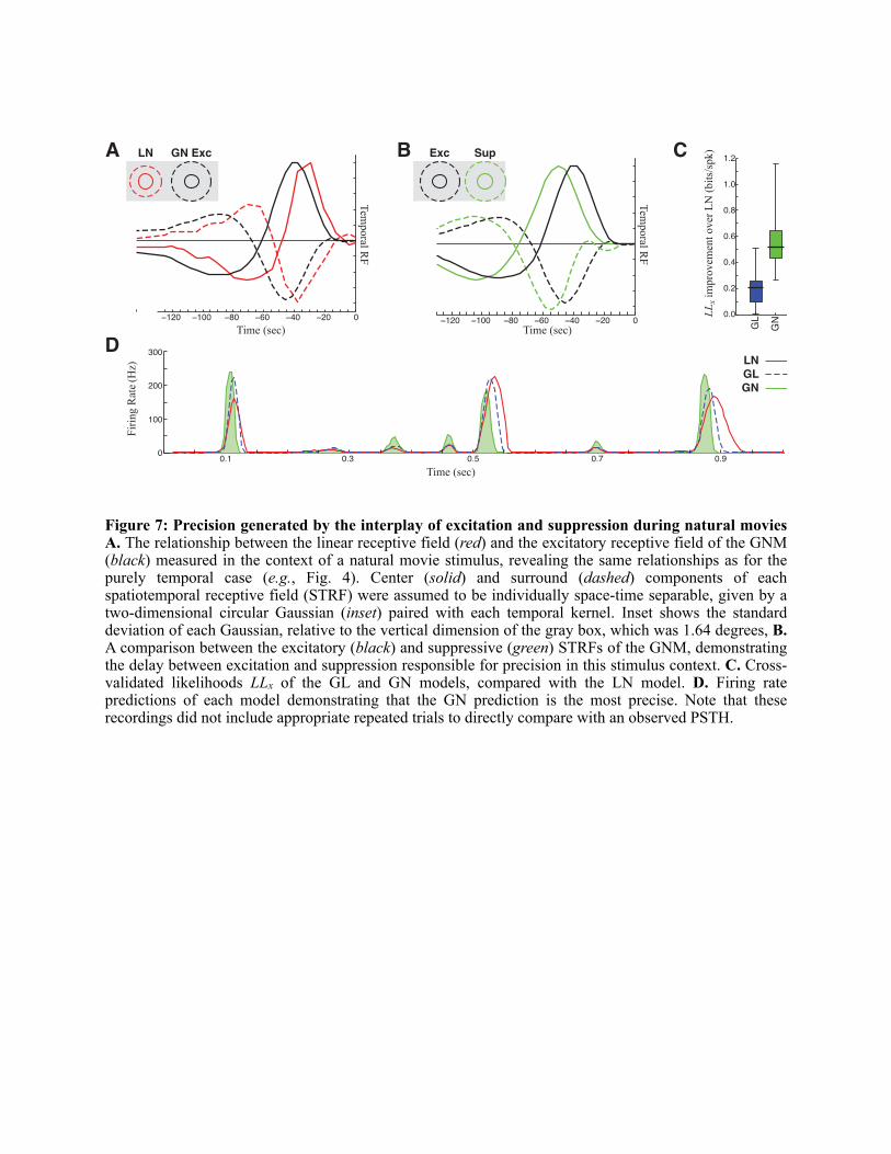
Figure 7: Precision generated by the interplay of excitation and suppression during natural movies A. The relationship between the linear receptive field (red) and the excitatory receptive field of the GNM (black) measured in the context of a natural movie stimulus, revealing the same relationships as for the purely temporal case (e.g., Fig. 4). Center (solid) and surround (dashed) components of each spatiotemporal receptive field (STRF) were assumed to be individually space-time separable, given by a two-dimensional circular Gaussian (inset) paired with each temporal kernel. Inset shows the standard deviation of each Gaussian, relative to the vertical dimension of the gray box, which was 1.64 degrees, B. A comparison between the excitatory (black) and suppressive (green) STRFs of the GNM, demonstrating the delay between excitation and suppression responsible for precision in this stimulus context. C. Cross-validated likelihoods LLx of the GL and GN models, compared with the LN model. D. Firing rate predictions of each model demonstrating that the GN prediction is the most precise. Note that these recordings did not include appropriate repeated trials to directly compare with an observed PSTH.

A B C

D!"#$%&'$() !"#$%&'$()

!!"%"#*+,-$#$./%,-$+%01%&2"/'3'*4)

GL

GN

!$#*,+56%7

8

!$#*,+56%7

8

Exc SupLN GN Exc

!"#$%&'$()

8"+".9%75/$%&:;) LN

GLGN

Figure 8. Elements of contrast gain control explained through the modulation of suppression relative to excitation. A. Simulated data is generated by the GNM using the previous excitatory and suppressive filters considered in previous figures (solid and dashed respectively) for the simulated “high contrast” condition. Low contrast is simulated by reducing the magnitude of the stimulus by a factor of two, while scaling the magnitude of the output of the suppressive term by a factor of three (dotted). Note that the kernel itself is not scaled (rather the magnitude of the signal after the suppressive nonlinearity, but this approximates the effect in (B). B. The spike-triggered average (STA) of the simulated data in high contrast (solid) and low contrast (dashed) conditions, demonstrating how the STA in high contrast becomes shorter latency and more biphasic: hallmarks of contrast gain control. The STA is scaled to have comparable variance for direct comparison of the shapes.

A

B

!"#$%&#'(

!"#$%&'"()*+

,-.-

!"

#"

!"#$%&#'(

!$#)*+,-%.

/0%1"-2$+'

!$#)*+,-%3!4

Part 1: Additional analysis of spike-triggered covariance models

As demonstrated in the main text, the spike-triggered covariance can identify the “subspace” of stimuli that a given neuron is sensitive to, but within this subspace, does not identify the same filters as the GN model. Here, we describe this STC analysis in detail, and offer additional analyses and comparison with the GN model. Construction of the “STC Model” The spike-triggered covariance matrix typically has a spectrum of eigenvalues shown in Fig. S1-1A for the example neuron considered in the main text, with one significant decreased-variance eigenvalue. The decreased-variance eigenvalue corresponds to a temporal filter that is delayed relative the STA (Fig. S1-1B), demonstrating a relationship between excitation and suppression similar to the GN model. In some cases, there is more than one significant eigenvalue, but the corresponding filters are usually not easily interpretable and do not seem to contribute significantly to response predictions. Because this pattern was consistent across every neuron in the study, we refer to the STA and the first decreased-variance STC filter as the STC filters. [Note that we project out the STA in calculating the spike triggered covariance matrix (e.g., Schwartz et al, 2006), although not doing so does not qualitatively change what we report here.] These filters define a stimulus subspace that is relevant to the neuronal response, which can be seen by projecting the location of each stimulus associated with a spike in this subspace (Fig. S1-1C, reproducing Fig. 5D, main text). This demonstrates that the STA identifies the direction of the center of mass of this “spike-cloud” (green arrow), and that there is decreased width of the cloud in the direction of the suppressive-STC filter (red arrows). Note that the width of the spike cloud projected into an arbitrary stimulus direction is unity (unit circle pictured), allowing for these comparisons. It is useful to further point out that the STC model identifies the same filters that would be found by an alternative technique: maximally-informative dimensions (MID), given the stimulus is Gaussian white noise (Sharpee, et al, 2004), as in this case. This was confirmed for a few cells using online software. Models based on STC analysis are Linear-Nonlinear (LN) cascades, although with a spiking nonlinearity F[g1,g2,…] that depends on the combined output of each linear filter, where gi(t) = s(t)*ki. The STC spiking nonlinearity can in principle be determined using the “histogram method”: just like in the one dimensional case (e.g., Chichilnisky, 2001), where the number of spikes in each bin (g1,g2) (Fig. S1-1C) is normalized by the number of times each combination occurred, resulting in the probability of a spike given the pair Pr{spk|(g1, g2)}. However, the higher dimensionality of the nonlinearity stretches the number of observed spikes over many more bins, making accurate estimation methods become more complicated. As a result, we applied recent techniques for non-parametric estimation of the nonlinearity (Rahnama Rad and Paninski, 2010), resulting in the measured spiking nonlinearity shown in Fig. S1-1D.

Supplementary Material, Part 1Butts et al. (2011)

1

Time (ms)

STA STC-1

Proj

ecte

d st

imul

us 2

(g2)

Projected stimulus 1 (g1)

Num

ber of spikes observed Proj

ecte

d st

imul

us 2

(g2)

Projected stimulus 1 (g1)

Firing Rate (H

z)

Eigenvalue Number-1 11 1

Varia

nce

A B C D

Figure S1-1: STC model of an LGN neuron in the context of SUN stimuli. A. The eigenvalues of the spike-triggered covariance matrix for the primary example neuron considered in the main text, demonstrating one significant decreased-variance eigenvalue (red arrow). B. The eigenvectors corresponding to the STA (green) and decreased variance (red): identical to Fig. 5A (main text). C. The density of spikes in the plane defined by the projections of the stimulus onto the subspace spanned by these two STC filters (color-labeled axes). All stimuli projecting into this plane form a distribution with a width of unity (black circle), making clear that the width of the spike distribution along the decreased-variance STC vector (vertical axis) is significantly decreased. D. The resulting two-dimensional spiking nonlinearity calculated by comparing the spike-density in (C) to the prior distribution of the stimulus in this plane, calculated using methods of Rahnama and Paninski (2010).

Note that this method is limited to two dimensions, because enough data does not exist to appropriately estimate nonlinearities with more dimensions (although see parametric estimation techniques used in V1 by, for example, Rust et al., 2005).

Structural differences and performance between the STC and GNM models Comparisons of the predictions of the resulting “STC model” from the LN, STC, and GN models (Fig. S1-2A) demonstrate that the STC model performs significantly better than the LN model -- capturing some degree of the precision in the LGN data -- but not nearly as well as the GNM, both for the neuron example considered, and for every neuron in this study (Fig. S1-2B). Because the STC model includes a second stimulus filter (STC-1) in addition to the STA, its improvement over the LN model demonstrates that this second filter generally has a predictive value. However, these two filters do not capture the interplay of excitation and inhibition that leads to the success of GNM prediction. At first glance, the inferior performance of the STC model might be surprising, because its filters span the same plane as the GNM filters (demonstrated in Fig. 6B, main text, and for all neurons in this study (Fig. S1-3). Specifically, because the STC models’ two-dimensional spiking nonlinearity is defined non-parametrically given the plane, the output of the model does not depend on the exact direction of these filters in the plane. Because the GNM filters largely project into this same plane, the superior performance of the GNM thus highlights important differences of the structure of these two models that extends beyond simply identifying the same relevant stimulus subspace. The GN model makes very specific, and much more restricting, sets of assumptions for how the two detected filters contribute to the neuronal firing. Specifically, each has a separate one-dimensional “internal” nonlinearity, and this is followed by a “PSC term” that leads to a further temporal convolution, followed by a second one-dimensional spiking nonlinearity (Fig. 2, main text). Such assumptions are much less general than STC model’s use of a higher-dimensional nonlinearity, which can capture arbitrary nonlinear interactions that are not applied across time, rather than those that are just separable into two one-dimensional nonlinearities as with the GNM. At the same time, while more general, the LN structure of the STC model cannot precisely capture the effects of the PSC term that follows the GNM’s internal nonlinearities that are then followed by a second [spiking] nonlinearity. As a result, while the GNM is likely less able to model arbitrary two-filter input-output functions, it can more accurately capture the type of structure resulting from the integration of inputs from other neurons. As described in the main text, the LNL(N) structure of the GNM is specifically designed to

Supplementary Material, Part 1Butts et al. (2011)

2

0.53 0.55 0.57 0.59 0.61 0.630

200

400

600

Time (sec) LLx improvement of STC model compared to LN model (bits/spk)

Firin

g R

ate

(Hz)

LNSTCGN

BA

0.0 0.5 1.0 1.5

0.0

0.5

1.0

1.5

LLx i

mpr

ovem

ent o

f GN

Mco

mpa

red

to L

N m

odel

(bits

/spk

)

Figure S1-2: Performance of the STC model. A. The cross-validated firing rate predictions of the LN (red), STC (magenta), and GN (green) models compared with the observed firing rate (black). This demonstrates that the STC model performs significantly better than the LN model -- capturing some of the precision of the neuron -- but not nearly to the level of the GNM. B. A comparison between the performance of the LN, STC, and GN models on a cell-by-cell basis (N = 21). Each individual point represents one neuron, and the horizontal position shows the improvement in LLx of the STC model over the LN model, and the vertical position shows the performance improvement of the GNM over the LN model. Because all but five points are to the right of the vertical red line, it shows that STC results in an improvement from the LN model for most of the neurons. However, the GNM model results in a much larger improvement over both the LN model (i.e., all points are well above the horizontal red line) and over the STC model (significantly above the dashed line. This improvement is for every neuron in the study. These results are summarized in Fig. 4C (main text).

emulate an inhibitory input from other neurons, with a temporal filter and associated nonlinearity representing its output, and the PSC term representing the IPSC. Furthermore, to aid in optimizing the model parameters, we restrict the internal nonlinearity to be monotonic, and the PSC term to be non-positive. [Again, such restrictions affect the generality of the model, but aid in that the optimization procedure is constrained to a “biologically realistic” parameter space.] Such assumptions also match observations in intracellular studied in the retina (Korenberg et al., 1989), which also suggest an LNL(N) model structure to describe retinal ganglion cell responses. The maximum-likelihood framework also allows for the incorporation of a spike-history term, which is estimated simultaneously with the other model parameters. This spike-history term further increases the likelihood of the GNM, because it captures the absolute refractory period and other temporal effects within 5 ms (Fig. 2C, main text). As a result, it affects the predicted spike patterning on small time scales, but has little affect on the PSTH (Fig. S1-2A). There is no clear way to incorporate a spike-history term into STC analysis directly, but we can use the STC filters to plug directly into GNM framework to simultaneously estimate the spike-history term as well the nonlinearities associated with each STC filter. The resulting nonlinearities (Fig. 5E, main text) suggest that the two-dimensional spiking nonlinearity (Fig. S1-1D) is largely separable into a saturating component along the direction of the STC and a bowl-shaped component perpendicular. However, while the resulting model has marginally better performance than the STC model without the spike-history term, it is clear that model performance it hurt by breaking the spiking nonlinearity into one dimensional separable components (data not shown). Note that this also means that parametric estimation of the STC’s spiking nonlinearity is not possible, and the full two-dimensional nonlinearity must be used to best predict the spike train using the STC filters. We conclude that STC analysis performs as it should: with little assumptions or effort, it can be directly applied to LGN data and identify the relevant subspace of stimuli that affect the neuron’s response. Likewise, for non-Gaussian stimuli, MID (Sharpee et al., 2004) can be used to accomplish the same task. However, it is clear that care must be taken in assigning particular importance to the particular stimulus directions identified by the STC analysis. This observation is consistent with an information-theoretic generalization of spike-triggered average and covariance analysis (iSTAC) (Pillow and Simoncelli, 2006), although in the case of the LGN data considered, we expect the most informative directions, considered separately, will be anchored to the STA. Only optimizing excitation and suppression together, in the context of an appropriate model structure, will yield the specific solutions of the GNM.

Supplementary Material, Part 1Butts et al. (2011)

3

Figure S1-3: The relationship between STC and GN model filters, reproduced from Fig. 5E (main text). A. The projection of the GN filters (exc: blue, inhib: green) onto the plane spanned by the STC filters (exc: black; suppressive: red) for the 21 LGN neurons in this study. Filters have a length less than one if there projections are not fully in the plane described by the two STC filters. B. A histogram of the angle between the excitatory and inhibitory filters for the GN model (diagrammed in the inset) for the 21 LGN neurons in this study, showing that excitation and inhibition are much closer to each other than in the STC model. C. A histogram of the angle between the excitatory GNM filter and the STA (diagrammed in the inset) for the 21 LGN neurons in this study.

A B

C

Latency

90

0

Exc

Inh

STC-1

STA

0 15 30 45 60 75 900

2

4

0 15 30 45 60 75 900

2

4

Angle between STA and GNM exc

Angle between GNM exc and inh

REFERENCES

Bonin V, Mante V, Carandini M (2005). The suppressive field of neurons in lateral geniculate nucleus. J Neurosci 25, 10844-10856.

de Ruyter van Steveninck R, Bialek W (1988). Coding and information transfer in short spike sequences. Proceedings of the Royal Society of London B, Biological Sciences 234, 379-414.

Hosoya T, Baccus SA, Meister M (2005). Dynamic predictive coding by the retina. Nature 436, 71-77.Korenberg MJ, Sakai HM, Naka K (1989). Dissection of the neuron network in the catfish inner retina.

III. Interpretation of spike kernels. J Neurophysiol 61, 1110-1120.Kouh M, Sharpee TO (2009). Estimating linear-nonlinear models using Renyi divergences. Network 20,

49-68.Lesica NA, Stanley GB (2006). Decoupling functional mechanisms of adaptive encoding. Network 17,

43-60.Paninski, L, Ahmadian Y, Ferreira D, Koyama S, Rahnama K, Vidne M, Vogelstein J, Wu W (2009). A

new look at state-space models for neural data. J Comput Neurosci Online (special issue on statistical analysis of neural data, Aug 1, 2009).

Pillow JW, Paninski L, Uzzell VJ, Simoncelli EP, Chichilnisky EJ (2005). Prediction and decoding of retinal ganglion cell responses with a probabilistic spiking model. J Neurosci 25, 11003-11013.

Pillow, JW, and Simoncelli, EP (2006). Dimensionality reduction in neural models: an information-theoretic generalization of spike-triggered average and covariance analysis. J Vis 6, 414-428.

Rahnama Rad K, Paninski L (2010) Efficient, adaptive estimation of two-dimensional firing rate surfaces via Gaussian process methods. Network 21,142-168.

Rust, NC, Schwartz, O, Movshon, JA, Simoncelli EP (2005). Spatiotemporal elements of macaque V1 receptive fields. Neuron 46, 945-956.

Shapley, RM, Victor, JD (1978). The effect of contrast on the transfer properties of cat retinal ganglion cells. J Physiol 285, 275-298.

Sharpee T, Rust NC, Bialek W (2004) Analyzing neural responses to natural signals: maximally informative dimensions. Neural Comput 16: 223-250.

Supplementary Material, Part 1Butts et al. (2011)

4

Part 2: Model performance on simulated spike trains

Solving nonlinear modeling problems is inherently unconstrained, because nonlinear models can be arbitrarily complex, and a more complex model might always be found that offers the same or a better explanation of the data. Our approach was to constrain the types of nonlinearities to model known or suspected mechanisms in retinal and retinogeniculate processing. In the main text, we demonstrated that other common models do not offer as good of an explanation for the observed data compared with the Generalized Nonlinear Model (GNM). However, to provide additional evidence that the solutions found by the GNM are specific to the mechanisms hypothesized, here we use the same analyses on simulated data, created using different hypothesized mechanisms of retinal and retinogeniculate processing. We demonstrate that the results of the GNM reflect the true form of the underlying model, and compare them to the results of other common modeling methods.

Model 1: Integrate-and-fire model of LGN Neuron

First, consider one of the other common models for the generation of precision by retinal ganglion cells (RGCs) and LGN neurons, through an intrinsic “refractoriness” following a spike (e.g., Berry and Meister, 1998; Keat et al., 2001; Pillow et al., 2005). In this case, we generated data using the model proposed by Keat et al. (2001), which involves linear filtering by a receptive field combined with a “spike-history” term that makes the neuron refractory following a spike. Note that this model differs from the Generalized Linear Model (GLM) considered in the main text because it has a deterministic threshold, although additional noise terms are added to reproduce the variability of observed spike trains. We consider the published model of a cat LGN neuron (Fig. S2-1A) using parameters provided by M. Meister, and generated a long simulated spike train for parameter estimation and a unique repeated sequence for cross-validation.

Figure S2-1. Analysis of data generated by a leaky integrate-and-fire model with spike-refractoriness. A. Sample spike raster showing a simulated spike train in response to repeats of the same stimulus. B. The temporal receptive field of GLM closely matches the actual RF, in contrast to that of the LN (red) and GLM models (blue), compared with the receptive field used to generate the data (black dashed). C. The spike history term of the GLM model (blue) largely recovers that used to in generating the data (black dashed). D. The spiking nonlinearity of the LN (red) and GL (blue) models, relative to the distribution of all internal model terms g (dashed). This shows the GLM finds a spiking nonlinearity that is close to a hard threshold, corresponding to the integrate-and-fire mechanism used to generate the data. E. The cross-validated log-likelihood (LLx) of each model, shown as a box plot over the LLx’s calculated for each of 100 repeated cross-validation trials. F. STC analysis finds two significant filters that describe the model, one corresponding to the spike-triggered average (red) and a second “suppressive” filter (magenta), similar to those found for the observed LGN data (Fig. 6, main text).

!

" #$

% &

!"#$%

!"#$%&'(

)'*

&'$(#)$%*

&($+,-./#0

1

&'$(#)$%*

2+'3(45'%6,-7#3(-8(/

!"#$%&)'*

1

1'-'89#-.6(#):;*

!#).-<=#>8'6%*

'()'*

LN GL

GN

STC

1

3

""##)<'6%?%+3*

&'$(#)$%*

&($+,-./#0

1

'(&)*+,-./0+,!-----

+,./0-----

Supplementary Material, Part 2Butts et al. (2011)

1

Despite a difference in spike-generation mechanism between this model and the GLM, maximum likelihood estimation of the GLM reproduces the parameters of the simulation (Fig. S2-1B & C). In this case, the resulting spiking nonlinearity is nearly vertical (Fig. S2-1D), reflecting the hard threshold used to generate this data. The correspondence between parameters found by the GLM and those of the original integrate-and-fire model is an additional validation of a separate study finding the same model parameters between the GLM and leaky integrate-and-fire models measured on RGC data using maximum likelihood estimation (Paninski et al., 2007). We also tested other models fit to this simulated data, and report their cross-validated likelihood measured from the repeated stimulus segments, in comparison to that of the GLM (Fig S2-1E). As expected, the LN model performs quite poorly on this dataset, as it cannot capture the precision in this data. Also, the GNM model (i.e., with an added suppressive term) does not perform significantly better than the GLM. Finally, spike-triggered covariance (STC) analysis can produce a model that performs better than the LN model, but not nearly as well as the GL and GN models. It is important to note that STC finds two significant filters (Fig. S2-1F), despite the fact that only a single filter processed the stimulus when the data was generated. Of course, the second filter is improving the description over that of the LN model because it is capturing aspects of the spike-refractoriness, because spike-history cannot be directly incorporated into STC analysis.

Model 2: GN model of LGN Neuron

Second, consider simulated data generated by the GNM (using parameters fit to the example LGN neuron in the main text), where temporal precision is generated through the interplay of excitation and inhibition. The resulting fits to the this simulated data are nearly identical to those found in the main text (i.e., fit to real data). First, the GNM fit to the simulated spike train itself finds the parameters of the generating model quite accurately (Fig. S2-2A,B, & C). Second, both the LN and GL models have similar temporal receptive fields, resembling the spike-triggered average. Third, the spike-history term of the GLM again has a “relative refractory period” (Fig. S2-2C), even though in this case there is no spike-refractoriness in the generating model at these longer time scales. Finally, the STC model applied to the simulated data also finds identical filters to those found with real LGN data (Fig. S2-2D). As a result, the STC filters have the same relationship to the GNM parameters as described in the main text. Cross-validation finds the performance of the GNM much better than the other models considered, mirroring the results found when applied to the recorded LGN data (Fig. 4C, main text).

Figure S2-2. Analysis of data generated GNM with excitation and inhibition. A. The GNM fit (green) can reproduce the temporal receptive fields for excitation and inhibition that generated the data (black). B. Identically to the analysis of the recorded LGN neuron, the temporal receptive fields of the LN (red) and GLM (blue) model to not resemble those that generated the data (black), and adding a spike-history term as little effect on the measured temporal processing (compare red with blue). C. The GNM (green) reproduces the spike-history term that was used to generate the data (black), while the GLM incorrectly describes a long relative refractory period, just as the fits to the observed LGN neuron (compare to Fig. 2C, main text). D. STC analysis of the simulated data (magenta) reveals the exact same filters as when applied to the observed data (black dashed, reproduced from Fig. 6, main text). E. The LLx for the four models considered show a similar trend to as the real data, with GLM and STC model offering a marginal improvement over the LN model, and a large increase in performance of the GNM.

! "

#$

!"#$%&'()

!"#$%&#'(

!$#)*+,-%.

/%

5 15!"#$%&#'(

0)"1$23"'4*+5%1$+6$-

!"#$%&'*)'()

!!"%&7"4'8')1(

1

3

LN GL

GN

STC

!"#$%&*(

'*)

!"#$%&#'(

!$#)*+,-%.

/

!"#$%&#'(

&'"(+,-$&%#./00000000000%"#$%&00

!$#)*+,-%.

/

Supplementary Material, Part 2Butts et al. (2011)

2

Model 3: Retinogeniculate synapse model

Third, consider RGC spike trains generated by either model above (#1 or #2), and then filtered by a model of the retinogeniculate (RG) synapse (Carandini et al., 2007). This model sums retinal spikes using an EPSC kernel fit to data, and introduces another spike-threshold at the level of the LGN, and is similar to other models of retinogeniculate processing in the literature (Casti et al., 2008; Babadi et al., 2009). Such additional RG processing could potentially introduce additional nonlinearities that are not well-fit by any of the models considered, and thus we test to see if the conclusions described for models #1 and #2 hold in this more complicated scenario. We used several different parameters listed in Carandini et al. (2007), and focus on an example with typical analysis results (Fig. S2-3A). Note that this RG model did not necessary result in a realistic LGN spike train in every case, and the RG model likely would have to match a particular input RGC spike train, which was not reported. However, results reported here are typical of the RG models studied, and are also consistent with GN modeling applied simultaneous recordings in the retina and LGN, in a followup study in preparation (Butts and Casti, 2009). Mirroring the results without RG processing, when the input RGC spike train was generated by the “Keat model” (Model #1), the GLM performs as well as the GNM (Fig. S2-3B, left). In contrast, when the input RGC spike train was generated by the GNM (Model #2), the GNM model significantly outperforms the other models (Fig. S2-3B, right). In both cases, the STC model outperforms the LN model, but does not do as nearly as well as the GNM. As expected, the performance of all models was lower than when applied to these models without the RG processing. Despite the additional complexity of this cascade model, the GNM still finds the same relationship between putative excitatory and inhibitory filters (Fig. S2-3C). However, note that these filters do not match those that were used to generate the input RGC spike train (Figs. S2-1 and S2-2), as would be expected given that the RG model introduces additional temporal and nonlinear effects. How these filters change due to RG processing has been a subject of much recent study (Sincich et al., 2009; Rathbun et al., 2010; Wang et al., 2010).

Figure S3-3. Analysis of data generated using retinogeniculate model applied to input spike trains generated by models #1 and #2. A. An example of RG processing, showing 20 repeats of an input spike train (generated by model #2) and the resulting output spike train generated by model #2. B. The LLx of the LN, GL, GN, and STC models applied to a RG model with an input spike train generated by the “Keat model” (model #1, left) and the GNM (right). In the first case, the GLM has similar performance to the GNM, suggesting the absence of inhibition governing precision of this spike train. In the second case, the GNM outperforms the other models. Note the increased variability of the GNM, which uses a Poisson process to generate spike trains, and this variability is amplified by thresholding in the RG model. C. The temporal RFs for excitation (black) and suppression (dashed green) are different than those used to generate the input spike train (Fig. S2-2A), but still have the same relationship between excitation and delated inhibition.

In conclusion, we find that the GNM correctly identifies the underlying causes of LGN precision in the case of the three simulations described, meant to address common alternative models for LGN spike train generation. When the underlying model was generated with spike refractoriness (either directly in the LGN or through RG processing), the GLM -- which is a subset of the GNM -- performed equivalently. In contrast, when the underlying model involved the interplay of excitation and inhibition, the GNM significantly outperformed alternative models (as with recorded data, main text) and detected the correct relationship between the filters. By comparison, STC analysis, another common method of system identification, was also useful in identifying additional elements of LGN processing, although could not perform as well as the models that were more closely matched to the underlying generating models. Clearly, if the underlying generating models did not use spike-refractoriness, and/or did not have a form that was close to that of the GNM, it is likely that STC would be a much more effective analysis tool. These additional modeling studies are not meant to (and in fact cannot) encompass all possible nonlinear aspects of nonlinear processing in the RG system. However, by addressing the most common alternative explanations for the data, we contribute to the strength of the predictions in the main text: that precision in the LGN arises through

! " #

!"#$%&#'(

!$#)*+,-%.

/

LN GL

GN

STC LN GL

GN

STC

0

1

2

3$%&'()*+,&-.

/012(345)/012(

!!"%&0"1'2')3(

45%#'

!"#$%&'#()*&%+,("&-'(.$/,%*0&1234

5$%#$%&'#()*&%+,("&-'(.$/,%*0&6274

0

Supplementary Material, Part 2Butts et al. (2011)

3

the interplay of excitation and inhibition, either generated in the retina and filtered through the RG synapse, or arising at the level of the LGN directly.

Additional Method DetailsSimulations. Stimuli used for the modeling simulations consisted of 60,000 frames (500 sec) of Gaussian white noise, with the same variance and refresh as in the experiment. Cross-validation stimuli consisted of 1,200 frames (10 sec) of a unique Gaussian white noise stimulus, presented 100 times. The integrate-and-fire model was reproduced following Keat et al. (2001) using parameters provided by M. Meister that matched the cat LGN neuron described in this publication. The GNM model parameters used were found by fitting to the LGN neuron described in Fig. 2 (main text), and a spike train was generated from the firing rate predictions by a Poisson process. Finally, the model of the RG synapse was reproduced following Carandini et al. (2007), and all 7 sets of parameters reported in the paper were simulated. The examples shown (Fig. S2-3) used the 4th in the list, although similar results were seen for other parameter sets.

STC analysis. As described in the main text and Supplementary Material Part 1, STC analysis (e.g., Schwartz et al., 2006) was applied by first calculating the spike-triggered average (STA), and then calculating the spike-triggered stimulus covariance with the STA projected out. The overall average covariance (with the STA projected out) was subtracted from the spike-triggered covariance (Rieke et al, 1997), and the resulting matrix was subjected to eigenvalue decomposition, from which we extracted the “STC filter” with the highest change in variance. Note that applying STC in this way lead to two filters (the STA and first STC filter) that are orthogonal, which makes it straightforward to calculate the spiking nonlinearity. However, other variants were also applied, but these yielded the best performance. Given the two “STC filters”, the two-dimensional spiking nonlinearity F(k1*s, k2*s) was estimated using non-parametric analysis (Rad and Paninski, 2010), resulting a firing rate prediction used for measurement of the cross-validated likelihood on the cross-validation stimulus. References Cited (Supplementary Material only)Babadi B, Casti A, Xiao Y, Kaplan E, Paninski L (2010) A generalized linear model of the impact of direct and indirect

inputs to the lateral geniculate nucleus. J Vis 10:22.Berry MJ, 2nd, Meister M (1998) Refractoriness and neural precision. J Neurosci 18:2200-2211.Carandini M, Horton JC, Sincich LC (2007) Thalamic filtering of retinal spike trains by postsynaptic summation. J Vis

7:20 21-11.Casti A, Hayot F, Xiao Y, Kaplan E (2008) A simple model of retina-LGN transmission. J Comput Neurosci 24:235-252.de Ruyter van Steveninck R, Bialek W (1988) Coding and information transfer in short spike sequences. Proceedings of

the Royal Society of London B, Biological Sciences 234:379-414.Keat J, Reinagel P, Reid RC, Meister M (2001) Predicting every spike: a model for the responses of visual neurons.

Neuron 30:803-817.Paninski L, Pillow JW, Lewi J (2007) Statistical models for neural encoding, decoding, and optimal stimulus design. In:

Computational Neuroscience: Theoretical Insights into Brain Function (Cisek P, Drew T, Kalaska J, eds), pp 493-507: Elsevier Science.

Pillow JW, Paninski L, Uzzell VJ, Simoncelli EP, Chichilnisky EJ (2005) Prediction and decoding of retinal ganglion cell responses with a probabilistic spiking model. J Neurosci 25:11003-11013.

Rad KR, Paninski L (2010) Efficient, adaptive estimation of two-dimensional firing rate surfaces via Gaussian process methods. Network 21:142-168.

Rathbun DL, Warland DK, Usrey WM (2010) Spike timing and information transmission at retinogeniculate synapses. J Neurosci 30:13558-13566.

Rieke F, Warland D, de Ruyter van Steveninck R, Bialek W (1997) Spikes: Exploring the Neural Code. Cambridge, MA: MIT Press.

Schwartz O, Pillow JW, Rust NC, Simoncelli EP (2006) Spike-triggered neural characterization. J Vis 6:484-507.Sincich LC, Horton JC, Sharpee TO (2009) Preserving information in neural transmission. J Neurosci 29:6207-6216.Wang X, Hirsch JA, Sommer FT (2010) Recoding of sensory information across the retinothalamic synapse. J Neurosci

30:13567-13577.

Supplementary Material, Part 2Butts et al. (2011)

4