temporal properties of low power wireless links: modeling
TRANSCRIPT

Temporal Properties of Low Power Wireless Links:
Modeling and Implications on Multi-Hop Routing
Abstract
Recently, several studies have analyzed the statisti-cal properties of low power wireless links in real en-vironments, clearly demonstrating the differences be-tween experimentally observed communication prop-erties and widely used simulation models. However,most of these studies have not analyzed the temporalproperties of wireless links in depth. These proper-ties have high impact on the performance of routingalgorithms.
Our first goal is to study the statistical temporalproperties of links in low power wireless communi-cations. We study short term temporal issues, likelagged autocorrelation of individual links, lagged cor-relation of reverse links, and consecutive same pathlinks. We also study long term temporal aspects,gaining insight on the length of time the channelneeds to be measured and how often we should up-date our models.
Our second objective is to explore how statisticaltemporal properties impact routing protocols. Westudied one-to-one routing schemes and developednew routing algorithms that consider autocorrelation,reverse link and consecutive same path link laggedcorrelations. We have developed two new routing al-gorithms for cost link model: (i) a generalized Di-jkstra algorithm with centralized execution, and (ii)localized distributed probabilistic.
1 Introduction
Recent studies indicate profound differences betweenexperimentally observed properties of low power com-munication links and widely used simulation mod-els [1, 2, 3, 4, 5]. Nevertheless, most of these studieshave not performed in depth analysis of the tempo-ral properties of wireless links. These properties havestrong impact on the performance of many protocolsand localized algorithms used in low power networks,in particular, routing algorithms.
Our starting point is a study of statistical tempo-ral properties of links in low power wireless commu-nication systems. We emphasize on time dependent
properties, which have strong ramifications on rout-ing protocols. The results of the study are used toanalyze how statistical temporal properties impactrouting protocols. We studied one-to-one routingprotocols and provided several suggestions for proto-col designers using the insight gained from our anal-ysis. We have also developed new routing algorithmsthat consider autocorrelation, reverse link and con-secutive same path link lagged correlations. The firstalgorithm is a generalized Dijkstra algorithm withcentralized execution. The second algorithm is a lo-calized probabilistic algorithm with distributed exe-cution.
In our study, we do not consider packet losses in-troduced by traffic synchronization (concurrent traf-fic, contention based MAC). Nevertheless, our resultsare useful for two reasons. First, they apply directlywhen using contention free MAC protocols, like pureTDMA or pseudo-TDMA schemes [6]. Second, theyprovide a tight upper bound as to what is achievablewhen using contention-based MAC schemes.
2 Related Work
There is a large body of literature on temporal modelsof radio propagation that have influenced this work.The emphasis has been on the variability of signalstrength in proximity to a particular location [7].Small scale fading models based on Rayleigh and Ricedistributions are used for modeling localized timedurations (a few microseconds) and space locations(usually one meter) changes [7].
The differences between the classical models andour approach are numerous and include differentmodeling objectives (reception rate of packets vs.signal strength), our radios have different features(e.g. communication range in meters instead of km),we capture phenomena that is not addressed by theclassical channel models (asymmetry, correlations be-tween reception rate of links), we use different model-ing techniques (free of assumptions, non-parametricvs. parametric), and we use unique evaluation tech-niques (evaluation of multi-hop routing).
More recently there have been many empirical
1

0 2 4 6 8 10 120
1
2
3
4
5
6
7
8
9
Distance (m)
Dis
tanc
e (m
)
34
35
33
37
36
42
44 43
38
50
39
51
40
52 46
31
49
47
41
48
45
55
32
54
53
15
30
29
8
25
24
23
27
28
26
7
22
18
19
21
20
17
9
11
2
1
4
16
8
3
5
10
13
14
12
Figure 1: Layout of the nodes
studies with deployments in several environments us-ing low-power RF radios [1, 2, 3, 4, 5]. Majority ofthese studies used the TR1000 [8] and CC1100 [9]low power RF transceivers (used by the Mica 1 [10]and Mica 2 [11] motes respectively). However, mostof these studies concentrate on analyzing the spatialcharacteristics of the radio channel and do not ana-lyze the temporal variability of link quality over ex-tended periods of time. Zhao et al. [2] performedsome temporal analysis using an array of nodesplaced in a straight line with two hour experiments.They demonstrated heavy variability in packet re-ception rate for a wide range of distances betweena transmitter and receiver. Furthermore, Cerpa etal. [4] used heterogeneous hardware platforms con-sisting of Mica 1 and Mica 2 motes in three differentenvironments to collect comprehensive data aboutthe dependency of reception rates over time with re-spect to a variety of parameters.
There are also several important empirical studiesusing medium-power RF radios in indoor and out-door environments [12, 13]. These studies use 802.11wireless radios. Aguayo et al. [12] measured the tem-poral variability of the packet reception rate for veryshort time scales (from 10 ms to 10 seconds) showingthat the packet loss rate for all links could be consid-ered independent for very small time scales (10 to 100ms), and then start deviating for some percentage oflinks at larger time scales. Draves et al. [13] com-pared different link quality estimation metrics, show-ing that the ETX metric [14] performs significantlybetter than hop-count and packet pair in static wire-less environments.
There are three major differences between the anal-ysis and evaluation developed in this paper and theprevious work. The first is that we study the impactof a significantly large number of factors that impactthe quality of wireless links over time and attemptto model not only isolated pairs of transmitters andreceivers, but also the correlation between differentpairs and different subsets of links with significantlylarger time scales (from 1 sec to several days). The
second major difference is that we have developed anew link quality metric that more accurately mea-sures the impact of the temporal variations of thewireless channels. Finally, using the knowledge builtwith our analysis, we implemented two new routingalgorithms that take advantage of our findings.
All of our techniques use non-parametric proce-dures. In particular, we directly leverage on smooth-ing and density kernel estimators [15, 16].
3 Experimental Methodology
We performed experiments using the SCALE wire-less measuring tool [4]. The basic data collectionexperiments work as follows. Either a single desig-nated node or a group of nodes transmit a certainnumber of packet probes (one transmitter at a timein the case of multiple transmitters). Each probepacket contains the sender’s node id and a sequencenumber. The rest of the nodes record the packetsreceived from each neighbor and keep updated con-nectivity statistics, using the sequence numbers todetect packet losses.
All experiments were conducted in an indoor office-like setting of approximately 20m by 20m. A totalof 55 Mica 1 mote [10] nodes, which uses the RFMTR1000 radio chip [8], were placed in a grid structurein the environment at approximately 1m distances.The layout of the nodes is shown in Figure 1.
We collected four types of data sets:Data set A. A single node broadcasts a packet ev-
ery second, all other nodes record the received pack-ets for a period of 24 hours. The purpose of this dataset was to establish the behavior of links over an ex-tended period of time. Four different nodes (10, 23,44, and 54) were selected as the broadcasting node.
Data set B. Node 23 broadcasts a packet everysecond, all other nodes record received packets for aperiod of 96 hours. This data set is used to determineif there is cyclical patterns in the link quality overmultiple days.
Data set C. Node 23 broadcasts a packet eachsecond to all other nodes in the network for a periodof 30 hours, where the packet size rotates in 10, 15,20, 30, 40, 80, 120, 135, 145, 150, 155, 170 and 190bytes. A packet of each size is sent every 13 seconds.The set is used to determine the impact of the packetsize on link quality.
Data set D. All nodes broadcast a packet one at atime in round robin fashion with one second intervalsbetween nodes for 48 hours. A packet is broadcastedby each node every 55 seconds. We collected two ofthese traces, the first one with round robin using nodeid sequence of 1, 2, . . . 55, and the second one with a
2

0 1000 3000 5000
020
4060
8010
0
Link 23 −− 43
Time (minutes)
Rec
eptio
n R
ate
(0−
100%
)
(a) RR: 48.02% RNP:1189.6
0 1000 3000 5000
020
4060
8010
0
Link 23 −− 24
Time (minutes)
Rec
eptio
n R
ate
(0−
100%
)(b) RR: 95.36% RNP:1.0491
0 1000 3000 5000
020
4060
8010
0
Link 23 −− 32
Time (minutes)
Rec
eptio
n R
ate
(0−
100%
)
(c) RR: 86.39% RNP:4.5673
0 1000 3000 5000
020
4060
8010
0
Link 23 −− 44
Time (minutes)
Rec
eptio
n R
ate
(0−
100%
)
(d) RR: 79.86% RNP:1.9175
Figure 2: Aggregate of reception rate by minute.
random node id sequence.
4 Temporal Properties
In this section we analyze several individual andgroup link properties of wireless links in our exper-iments. Our goal is to improve our qualitative andquantitative understanding of the link temporal prop-erties, providing intuition for network design and op-eration, as well as statistically sound conclusions.
4.1 Single Link Autocorrelation
The most common measure for the quality of linksis the percentage of received packets over a certainperiod of time, reception rate (RR). We will see thata better measure is to consider the average number ofpackets that must be sent before a packet is received.We will refer to this value as the required number ofpackets (RNP). Commonly, it is assumed there is areverse relationship between RNP and RR. However,temporal correlations often invalidates this.
For example, consider the four links shown in Fig-ure 2. In this case, we show the aggregated receptionrate (by minute) of the data from set B. In Figure2(a) we see a link with an average reception rate of48.02%. This link is highly unreliable and the re-quired number of packets (with constant back-off)will be high (1189.65), even though there are minuteswhere the link is reliable. In Figure 2(b)) we show alink that has very high reception rate (95.36%). Inthis case, while a few messages were not received thelink was completely reliable with very low requirednumber of packets (1.05). Consider the medium qual-ity links shown in Figures 2(c) and 2(d). The first linkhas a RR of 86.39% and the second link has a RR of79.86%. When using RR as a quality metric, clearlythe first link is better than the second. Surprisingly,when using RNP, the second link is much better thanthe first. The reason of this counterintuitive result
RR−1 1-1.1 1.1-1.2 1.2-1.5 1.5-2 2-5 5-10
Cons. 0.970 0.695 0.661 0.658 0.607 0.555
Table 1: 1/RR and RNP Consistency
is due to the fact that the RR metric does not takeinto account the underlying distribution of the losses;short periods of zero RR in any particular time inter-val will trigger the RNP to higher values, even thoughthe average RR might still be higher than the otherlink in the same time interval. As a result of this in-consistent behavior, the required number of packetsprovides a better picture of the usefulness of the link.
We statistically analyze the relationship betweenthe reception rate and the required number of pack-ets using data sets B and D to fully characterize theusefulness of moderate links. Fig. 3 shows the rela-tionship between RNP and RR in log scale. If theunderlying distribution of packet losses correspondsto a random uniform distribution, we would expect aone-to-one relationship between RNP and RR. Fromthe figure we clearly see this is not the case. Perhapsmore importantly, using RR as the main evaluationof link quality estimation can lead to gross overesti-mation of the quality of certain links. It is clear thatthere exist many pairs of links i and j where one linkhas i has both lower RR and lower RNP than link j.
Fig. 3(b) shows the CDF of RNP as a function ofRR for different percentages of population below eachcurve. We observe that most of the values tend toconverge at very high or very low RR values, but thevalues of 10% < RR < 90% tend to be quite spread.
The above figures show that the RR is not a pre-cise estimator for the absolute RNP values in a sig-nificant range. Table 1 shows the consistency levelsbased on different 1/RR value groups. In our study,our criteria of consistency is defined as the probabil-ity of the 1/RR estimator to rank the links in thesame ranking order as their RNP values within eachgroup, or in other words, the relative difference withrespect to other links (not the absolute value). The
3

0 1 2 3 40
0.5
1
1.5
2
2.5
3
3.5
LOG(1/RR)
LOG
(RN
P)
(a) Links characterized by their 1/RR and RNPvalues
0 1 2 3 40
0.5
1
1.5
2
2.5
3
3.5
LOG(1/RR)
LOG
(RN
P)
12.5%25%50%75%85.2%
(b) CDF of RNP as function of 1/RR (doublelogarithmic scale)
Figure 3: RNP as a function of 1/RR
0 0.98 1.98 2.98 3.98 0
4.43
9.10
13.76
0
0.05
0.1
0.15
0.2
0.25
Dis
tanc
e (m
)
LOG(Expected # of Messages)
PD
F
(a) RNP and link length PDF
0
0.2
0.4
0.6
0.8
1
1 10 100 1000 10000 100000
Con
ditio
nal P
roba
bilit
y
Autocorrelation Time Shift (seconds)
CP vs Tau
good 1->1medium 1->1
bad 1->1good 0->0
medium 0->0bad 0->0
(b) CP as a function of τ
Figure 4: RNP and Autocorrelation
consistency for all links is 0.959. However, from thetable we observe that the RR measure is only a con-sistent RNP estimator for the higher quality link (RR> 90%), and the consistency decreases rapidly afterthat. Note that a 50% consistency estimator is asuseful as flipping a coin.
The likelihood of the required number of packetsfor a given distance is presented in Figure 4(a). Weused data sets A and B for analysis. The figure illus-trates that when the distance between the transmit-ter and receiver is low, there is a high likelihood thatthe RNP will be low. However, as distance increases,we do not see a corresponding increasing trend inRNP as would be expected if there exists a strongrelationship between the two factors. Often for anygiven distance there is a non-trivial likelihood thatthe RNP will be fairly low. As a result, the distancebetween two radios is not the determining factor in
the quality of the link.
Next, we analyze the autocorrelation of three qual-itatively different types of links (good, medium, bad)by using conditional probabilities (CP) of two events,a packet reception after a packet reception (1→1) anda packet loss after a packet loss (0→0) for differenttime intervals (τ : 2n seconds with n : 1, 2, . . . 15). Weobserve in Figure 4(b) that good links tend to havea very high and very low CP for the 1→1 and 0→0,respectively over very long periods of time. This in-dicates that good links are quite stable. On the otherhand, bad links are stable as well for shorter periodsof times, but their properties tend to disappear oncewe go into longer periods of time (in the order of ∼9hrs). Medium links tend to have higher correlationfor successful packet reception (1→1) than for packetlosses (0→0). In the latter case, the autocorrelationdrops for the larger time intervals.
4
0
0.2
0.4
0.6
0.8
1
0 20 40 60 80 100
Con
ditio
nal P
roba
bilit
y
Reception Rate (0-100%)
CP (1 -> 1) vs RR (good)
(a) good
0
0.2
0.4
0.6
0.8
1
0 20 40 60 80 100
Con
ditio
nal P
roba
bilit
y
Reception Rate (0-100%)
CP (1 -> 1) vs RR (medium)
(b) medium
0
0.2
0.4
0.6
0.8
1
0 20 40 60 80 100
Con
ditio
nal P
roba
bilit
y
Reception Rate (0-100%)
CP (1 -> 1) vs RR (bad)
(c) bad
0
0.2
0.4
0.6
0.8
1
0 20 40 60 80 100
Con
ditio
nal P
roba
bilit
y
Reception Rate (0-100%)
CP (0 -> 1) vs RR (good)
(d) good
0
0.2
0.4
0.6
0.8
1
0 20 40 60 80 100
Con
ditio
nal P
roba
bilit
y
Reception Rate (0-100%)
CP (0 -> 1) vs RR (medium)
(e) medium
0
0.2
0.4
0.6
0.8
1
0 20 40 60 80 100
Con
ditio
nal P
roba
bilit
y
Reception Rate (0-100%)
CP (0 -> 1) vs RR (bad)
(f) bad
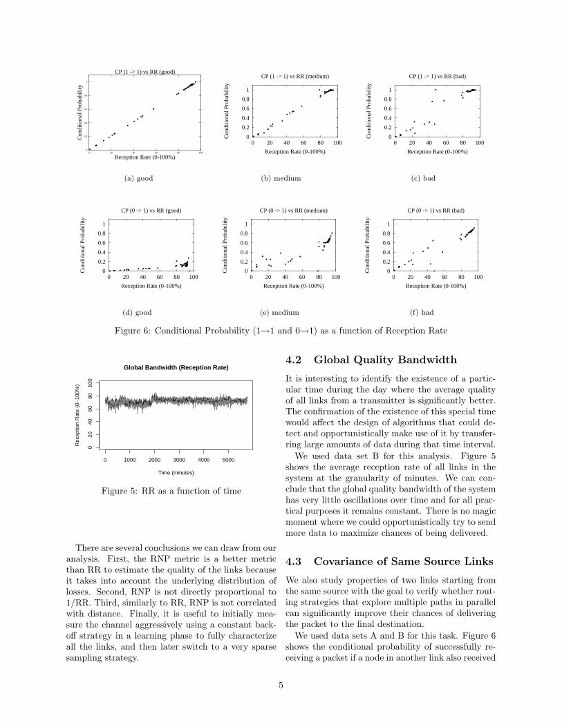
Figure 6: Conditional Probability (1→1 and 0→1) as a function of Reception Rate
0 1000 2000 3000 4000 5000
020
4060
8010
0
Global Bandwidth (Reception Rate)
Time (minutes)
Rec
eptio
n R
ate
(0−
100%
)
Figure 5: RR as a function of time
There are several conclusions we can draw from ouranalysis. First, the RNP metric is a better metricthan RR to estimate the quality of the links becauseit takes into account the underlying distribution oflosses. Second, RNP is not directly proportional to1/RR. Third, similarly to RR, RNP is not correlatedwith distance. Finally, it is useful to initially mea-sure the channel aggressively using a constant back-off strategy in a learning phase to fully characterizeall the links, and then later switch to a very sparsesampling strategy.
4.2 Global Quality Bandwidth
It is interesting to identify the existence of a partic-ular time during the day where the average qualityof all links from a transmitter is significantly better.The confirmation of the existence of this special timewould affect the design of algorithms that could de-tect and opportunistically make use of it by transfer-ring large amounts of data during that time interval.
We used data set B for this analysis. Figure 5shows the average reception rate of all links in thesystem at the granularity of minutes. We can con-clude that the global quality bandwidth of the systemhas very little oscillations over time and for all prac-tical purposes it remains constant. There is no magicmoment where we could opportunistically try to sendmore data to maximize chances of being delivered.
4.3 Covariance of Same Source Links
We also study properties of two links starting fromthe same source with the goal to verify whether rout-ing strategies that explore multiple paths in parallelcan significantly improve their chances of deliveringthe packet to the final destination.
We used data sets A and B for this task. Figure 6shows the conditional probability of successfully re-ceiving a packet if a node in another link also received
5

1 2 4 8 16 320
0.5
1
Asymmetric Links: CRNP > RNP
Tau
Per
cent
age
AllRNP > 51.3 < RNP < 5RNP < 1.3Useful Links (20%)Useful Links (40%)
(a) Required Number of Packets
1 2 4 8 16 320.2
0.4
0.6
0.8
1Asymmetric Links: CRR > RR
Tau
Per
cent
age
(b) Reception Rate
Figure 7: Percentage of inconsistent links vs time
0 200 400 600 800 10000
500
1000
1500
Sum of One−way RNPs
Act
ual R
NP
(a) Sum of One-way RNPs < 1000
2 3 4 52
4
6
8
10
Sum of One−way RNPs
Act
ual R
NP
(b) Sum of One-way RNPs < 5
Figure 8: Actual RNP cost as a function of the sum of one-way RNP estimator
it (1→1), and the conditional probability of success-fully receiving a packet if a node in another link didn’treceive it (0→1). We used three qualitatively differ-ent links (good, bad, and medium) to establish a com-parison. Figure 6(a) shows that when a high qualitylink received a packet, most likely all other links willreceive the same packet almost directly proportion-ally to the reception rate. Figures 6(b) and 6(c) showthat when medium and bad quality links receive apacket from the source, the high quality links willalso receive the same packet with very high proba-bility. Figure 6(d) shows that when a good qualitylink does not receive a packet, with very high proba-bility none of the other links will receive that packeteither, even other high quality links. Therefore, thereis very little incentive in spending more energy andbandwidth by trying to exploit multiple paths con-currently because chances are that none of the nodeswill receive the packet. Figures 6(f) and 6(e) showthat when bad and medium quality links do not re-ceive the packet from the source, high quality linksstill have high chances of receiving it (as intuition
would indicate).Our main conclusion from this analysis is that
when routing data using high quality links, we shoulduse single path routing strategies and abandon multi-ple concurrent paths strategies because they providevery little benefit for the increased cost in terms ofenergy consumption and contention for resources.
4.4 Forward and Reverse Link Corre-
lation
In this subsection, we study the forward and re-verse link properties between a pair of nodes. Theseproperties are important for any protocol that usestwo-way communication between source and destina-tion, and in particular, when using hop-by-hop re-liable schemes with acknowledgements (acks). Thekey questions we try to answer are when are thebest times to forward and acknowledge reception ofa packet and what is the best metric to measure thecombined data forward and reverse acknowledgmenttotal cost.
6

0
0.2
0.4
0.6
0.8
1
1.2
1.4
1.6
1.8
0 50 100 150 200
Ave
rage
Req
uire
d N
umbe
r of
Pac
kets
Packet Size (bytes)
RNP vs Packet Size
(a) Average Reception Rate
0
0.2
0.4
0.6
0.8
1
0 50 100 150 200
Ave
rage
Rec
eptio
n R
ate
(0-1
00%
)
Packet Size (bytes)
Reception Rate vs Packet Size
(b) Average RNP
0
0.0005
0.001
0.0015
0.002
0.0025
0.003
0 0.1 0.2 0.3 0.4 0.5 0.6 0.7 0.8 0.9
Rat
e of
cha
nge
Average Reception Rate
Slope 15-170
(c) Rate of Change
Figure 9: Variation as a function of the Packet Size
For this analysis we use data set D. The first ques-tion we address is whether there is any advantages inimmediately sending an ack from the 1-hop destina-tion to the source for a packet just received. We callthe conditional required number of packets (CRNP)and the conditional reception rate (CRR) the cost inthe reverse direction (acknowledgment from destina-tion to source), conditional upon successfully receiv-ing a packet in the forward direction. Figs. 7(a) and7(b) show the percentage of links that have higherCRNP and CRR in the reverse direction in compar-ison with their overall RNP and RR in the reversedirection when a packet was successfully received inthe forward direction as a function of the time waitedto send the ack back (τ , measured in seconds). Weanalyzed six qualitatively different classes of linksthat are of potential interest for routing purposes:all links, high quality links (RNP < 1.3), mediumquality links (1.3 < RNP < 5), low quality links(RR> 5) and links with high distance over RNP ratiosclassified into two groups (top 20% and top 40%).In Fig. 7(a) we see that for all links in general andfor almost all classes of links (except for the top 40%of useful links), the percentage of links with CRNPlarger than RNP is quite small, and it is smaller whenthe ack is sent back as soon as possible (the smallerthe RNP the better). Similarly, in Fig. 7(b) we seethat the percentage of links with CRR larger thanRR is higher for all links in general and almost allclasses of links (except the top 40% and bad links)when the ack is sent back immediately. Therefore,there is a significant advantage to send ack signals inthe first few seconds after reception. The advantagediminishes as waiting time increases.
The other aspect we are interested is to determinethe actual cost of a link when using hop-by-hop acks,and whether this cost could be estimated by the sumof the individual RNP in the forward and reverse di-rection, without requiring on-line measurement of theactual conditional cost. Considering only the RNPs
in each link direction may not necessarily determinethe best quality link if the forward and reverse direc-tion present different levels of correlation for differ-ent links. Figure 8 shows the relationship betweenthe sum of each individual RNP in each direction,and the actual RNP cost for all links when sendingthe acknowledgment immediately. In particular, wecould observe from Fig. 8(b) that the sum of one-wayRNPs is quite correlated with the actual link cost,with stronger correlation for smaller RNP values. Inaddition, the percentage of consistency (as defined insection 4.1) for this estimator is very high (96.2%).Therefore, the sum of RNPs is almost always a goodindicator of overall quality of the link.
We conclude that there is significant benefit to ac-knowledge packets immediately because we increasethe chances of the acknowledgement being received.We also conclude that an accurate cost metric couldbe well estimated using only the individual RNP val-ues of each direction because the number of inconsis-tent links is not significant.
4.5 Packet Size
In this section, we analyze how the packet size affectsthe RR and the RNP. Each packet transmitted hasa minimum fixed overhead provided by the startingsymbol sequence, the radio header and the CRC. Thiscost is fixed and independent of the packet payloadsize. Our main motivation is to improve transmissionefficiency by having proportionally less overhead peruseful bit transmitted in the payload.
Using data set C, the first question we try to an-swer is to whether there is a fundamental trend orchange that occurs for RR and/or RNP as a func-tion of packet size globally in the network. Figures9(a) and 9(b) show the average RR and RNP as afunction of different packet sizes for all links in theexperiment. We see that the average RR slowly de-crease and the RNP slowly increases until a packet
7

(a) RNP Cost (b) RNP Cost < 5 (c) RR Cost (d) RR Cost < 5
Figure 11: Link Cost for 2-hop Forwarding Links
0 20 40 6010
−6
10−4
10−2
100
102
Tau
Log(
L1)
All PairsRNP < 1.251.25 < RNP < 3RNP > 3Useful Links
Figure 10: L1 RNP differences as a function of time
size of 125 bytes.
The next aspect we would like to explore is to un-derstand whether the change in packet sizes affect alllinks equally or if there is any relationship as a func-tion of average RR. Figure 9(c) shows the relation-ship between the rate of change of the average RR asa function of the packet size for each pair of nodes inthe experiments. The factor m on the y-axis corre-sponds to the slope of the linear interpolation of theaverage reception rates and different packet sizes foreach link. All the different m coefficients are plot-ted as a function of the average reception rate forall packet sizes. We see that links with very low (<20%) or very high (> 80%) RR are less affected by thechange in packet size. Links with medium RR show amuch larger variation. The quality variation of thesegroup of links is strongly affected as we increase thepacket size.
We can conclude that using larger packet sizes iscertainly better in terms of efficiency by minimiz-ing the overhead per useful bit transmitted withoutsignificantly increasing the RNP. Larger packet sizescould be use for opportunistic aggregation of data inintermediate nodes when multiple data packets areintended for the same destination, and when trans-
mitting large amount of information.
4.6 Temporal Consistency of Links
It is also important to analyze long term correlationsand the uniformity of links. The main motivation inthis section is to determine how stable the links areand how often we have to update estimates abouttheir quality.
Figure 10 shows the L1 norm of relative RNP dif-ferences for the five qualitatively different classes oflinks as a function of time (measured in hours). Notethat y-axis follows a logarithmic scale and the finestructure of the differences is not completely visible.However, a number of conclusions is apparent andthe most important features are well captured usinglogarithmic scale.
We see that the most stable links are the low RNPlinks with very small differences 10−3 from the av-erage over extended periods of time. An interestingresult is that the variability of the high distance/RNPlinks (useful links) is also well below the average ofall the links. Their change rate is less than 1% over60 hours. Finally, we see that links with RNP > 3change at very rapid pace. However, since most ofthe links in our experiments were good links, the av-erage variability for all links is skewed more heavilyby the stability of the good links.
So, the stability of the links vary drastically de-pending on the quality of each link. Importantly,good quality links (high RR, low RNP) tend to bevery stable over time. This is an additional reasonwhy those high quality links are exactly the ones thatshould be used in routing traffic.
4.7 Correlation Among Links on the
Same Path
In this section, we study the link properties betweentwo links in the same forwarding path. These prop-erties are important since they can determine the to-
8

Algorithm 1 Two-Hop Correlation Shortest PathAlgorithm
1: procedure CSP(W, i) . connectivity matrix andsource node
2: V = all n ∈ W − i . init candidate set3: InitState(W,i) . init all the state variables4: while V 6= ∅ do . candidate nodes available5: u =RemoveBest(V ) . based on shortest
distance6: for all n ∈ W (u) do
7: for all p ∈ W (u) do . all neighbors of u8: UPDATE(u, n, p). update direct paths9: end for
10: for all p ∈ W (n) do . all neighbors of n11: UPDATE(n, p, u) . update other12: end for
13: end for
14: end while
15: end procedure
16: procedure Update(s, d, p)17: D(s, d, p) = BestDist(s, p) + W (s, d, p)18: P (s, d, p) = BestPath(s, p) + s
19: if MD(d) > D(s, d, p) then . relaxationcondition
20: MD(d) = D(s, d, p)21: MP (d) = P (s, d, p)
22: end if
23: end procedure
tal number of hops we need to gather information tomake sound routing decisions.
We are interested in establishing the actual cost ofa link when forwarding the packet in the path uponsuccessful reception from the previous hop. Consid-ering only the RNP of the previous hop link to choosethe link for routing purposes may not necessarily de-termine the best link if the next hop link presents dif-ferent levels of correlation for different previous hoplinks. Figure 11 shows the relationship between thesum of each individual RNP and RR in each hop,and the actual RNP cost for all links when forward-ing the packet immediately to the next hop. We seefrom Fig. 11(b) that the sum of one-way RNPs in theforward direction is almost always greater than theactual cost of the forwarding path. The gains whenusing conditional RNP in the forwarding path aremore significant than the one obtained in Section 4.4and should be considered in order to establish theright quality metric for routing decisions.
We conclude that the link quality metric for rout-ing should not only consider the RNP of individuallinks, but the actual conditional RNP based on theprevious hop to get more accurate results with rout-ing. Combining this result with the results of Sec-
tion 4.4, means that when we are using a hop-by-hopacknowledgment mechanism it would be convenientto use an implicit acknowledgement strategy; i.e. for-ward the packet to the next hop immediately andcombine it with a flag to indicate an ack to the pre-vious hop from which we receive the packet.
5 Impact on Routing
In this section, we present some of the lessons learnedin our previous analysis that could impact the designof routing algorithms and two new routing algorithmsthat could be used depending on the level of dynamicsexpected by the operation of the system.
5.1 Lessons Learned
There are several lessons learned that can impact theway we do routing in sensor networks. While RR isthe most intuitive metric to measure link quality, it isnot always correct, and RNP should be used instead.High quality links are very good and quite stable overtime. These links consistently rank among the toplinks over long periods of time. Therefore, centralizedsolutions are attractive because they allow to calcu-late an optimal solution to the shortest path routingproblem and have low overhead in terms of the to-tal number of control packets required to update therouting tables.
Nevertheless, there are cases when a centralized so-lution may not scale. For example, the network maynot have enough number of good links to route allpackets to the destinations. In addition, increasinglevels of dynamics might be introduced by nodes fail-ing, and/or by applying a sleeping scheduling mech-anism on a subset of the available nodes [17, 18].
5.2 Centralized Routing Algorithm
Based on the analysis performed in Section 4, weshowed that link correlations in the reverse-forwardlinks and the consecutive links on the same path aresignificant and cannot be ignored. Therefore, any op-timal solution of the shortest path routing problemshould also consider the correlations among links.
We have developed a generalized version of the Di-jkstra algorithm that calculates the shortest path andconsiders correlations among links on the same path.The input of the algorithm consists of the source nodeid i and a 3-dimensional connectivity matrix indexedwith variables source (s), destination (d), and previ-ous hop (p) that have the following values:
9

3
1
5
1
11 a
b
c
d
0
3
�1 M
(a) Step 1
3
1
5
1
11 a
b
c
d
0
2
�1 6
(b) Step 2
3
1
5
1
11 a
b
c
d
0
2
�1 5
(c) Step 3
Figure 12: Operation of the Two-Hop Correlation Shortest Path Algorithm
Wi,n,i =
{
cRNPi,n ∀ n neigh i,
∞ otherwise.(1)
Ws,d,p =
{
sRNPp,s,d ∀ ∃ (s, d, p) tuples,
∞ otherwise.(2)
The pseudo code is shown in Algorithm 1. The ar-guments needed are the W matrix and the sourcenode i. The InitState call in line 3 initializes allthe state variables. For the source i, MD(i) = 0,MP (i) = ∅, for the neighbors n of source i, MD(n) =W (i, n, i), MP (n) = i, and for the rest of the (s, d, p)tuple MD(s) = D(s, d, p) = ∞, MP (s) = P (s, d, p) =∅. The while loop that goes from lines 4 to 14 showsthe main algorithm that is quite similar to standardSP Dijkstra. The differences are in the additionalfor loop in lines 10 to 12 and in the modified UP-
DATE procedure. Due to the correlations that mayexist among links on the same path, the addition of anew node from the candidate set may affect previousroutes to nodes that are not directly connected to thenode being added to the covered set. In addition, werequire to keep additional path state information inorder to update the precedence matrix when a situa-tion like this arises.
Figure 12 shows an example of the algorithm inaction on a small four node network. The nodes arelabeled with letters, the numbers inside the nodesindicate the shortest distance (MD) known at eachstep, and the edges show the different link costs de-pending on which previous node the packet comesfrom. For simplicity, several edges have the samecost in both directions. Note that there might beseveral edges between each pair of nodes dependingon the previous hop (e.g. b → d cost is five if com-ing from a, and one if coming from c). Figure 12(a)shows the first step of the algorithm at initialization.The source node a is the only node in the defined
set (bold), the shortest distance (MD) to the directneighbors b and c is updated, and the distance ofall the remaining nodes (d) is ∞ (M in the figure).Figure 12(b) shows the next step of the algorithm.Node b is removed from the candidate set, and alltheir neighbor nodes are updated. The results so farare identical to standard Dijkstra. Figure 12(c) showsthe next step. When adding node c to the defined set(bold), this node does not have new direct neighborsfrom the candidate set. The standard Dijkstra algo-rithm would have stopped here. However, due to thehigh correlation with the link b → d, a better short-est path to d that goes from a → c → b is updatedwhen using our algorithm. The running time of the
algorithm is O(n3) for dense and O( n3
lognfor sparse
networks. It shows average improvements over thestandard Dijkstra algorithm between 11% and 24%on set of networks that are formed by subset of nodesin our network.
5.3 Distributed Routing Algorithm
There are some scenarios where a centralized solutiondoes not scale and distributed solutions are preferred.For example, there are several topology control al-gorithms [17, 18] that turn a subset of nodes off tosave energy. These mechanisms change the underly-ing topology, forcing a recalculation of the optimalpaths every time a node is turned off. Under theseconditions, distributed solutions that depend on lo-calized information may be more attractive.
We present a randomized distributed algorithm forsolving the routing problem between two nodes in thenetwork. We assume that nodes only know the RNPfrom other neighbors, and that packets include theaggregate RNP of the path (aRNP). This aRNP isthe sum of all the RNPs in the path with respect tothe original sender, and it is updated by each node inthe packet forwarding path. Only directly connectednodes know when a neighbor is down (turned itself off
10

and/or died). Source and destination nodes periodi-cally send traffic to each other, enabling data trafficin both directions. The most important assumptionwe make is that good (i.e. low RNP) end-to-end pathsare bidirectional as shown in section 4.4.
Each node maintains aRNP state for each (neigh-bor, sender) tuple. This state is updated every time anew packet from the sender is received via the neigh-bor. The aRNP estimated is calculated using an ex-ponential weighted moving average (EWMA) with αfactor of 0.01 (i.e. each new sample weighs 1% onthe current estimate). Upon reception of a packet,each node unicasts the packet to the next hop. Thenext hop is determined probabilistically based on theaRNP estimates to the destination (calculated usingprevious traffic coming from the destination as ex-plained above). The forwarding probability for eachnext hop candidate is given by the inverse of theaRNP for the (neighbor, destination) tuple dividedby the sum of the aRNP inverses of all next hopcandidate neighbors (neighbor, destination) tuples,all factors using a power factor δ. For instance, theprobability of forwarding the packet to neighbor a,with final destination D, and a . . . n possible next hopneighbor candidates is given by:
Pa =(1/aRNPa,D)
δ
∑
a≤i≤n (1/aRNPi,D)δ
(3)
6 Simulation Results
We conducted simulations using EmStar [19] to mea-sure the performance of our distributed algorithm inthe presence of node dynamics. We set up a 60-nodenetwork for our simulations, with node degrees vary-ing from 2 to 11, and with different link quality val-ues. The best link had an RNP of 1.0, and the worsthad an RNP of 6.387.
Each node in the simulation is initialized with theoptimal routes calculated using the algorithm de-scribed in section 5.2 using all available nodes in thenetwork. For each experiment, traffic is sent betweensource and destination with a constant bit rate. Ineach simulation run, we put 10% of the nodes to sleep(excluding source and destination), and then aftera period of time (12 minutes), another 10% of thenodes go to sleep and the previous dormant nodeswake up. Each time nodes go to sleep, the optimalroute between source and destination is re-calculatedinstantly (no overhead, ideal case).
We implemented in Emstar a series of modulesto simulate our distributed solution. LQE is theRNP link quality estimator implemented using themethodology described in the previous section. HBH,
0
10
20
30
40
50
60
0 10 20 30 40 50 60
Cen
tral
ized
Cos
t
Distributed Cost
Packet Cost Ratio
Figure 13: Total Packet Cost Central-ized/Distributed
is a simple hop by hop reliability scheme that im-plements a stop and wait protocol. Finally, MIN-RNP implements the distributed routing algorithmdescribed in section 5.3. We use a power factor δ oftwo for routing in our simulations.
The main performance metric we measured was theaverage total number of packets required to transmitone message back and forth between source and des-tination. Optimal routes tend to minimize the to-tal number of packets required to transmit reliablybetween source and destination, and thus minimizeenergy consumption. Fig. 13 shows the relationshipbetween the centralized optimal solution and our dis-tributed solution. From the graph we see that whenthe cost of the path is small, the difference betweenthe optimal and our distributed solution is not sig-nificant. When the path cost increases, the differ-ence increases as well. The relative efficiency of thedistributed case with respect to the centralized algo-rithm is 0.324 in the worst case. The convergencetime of the algorithm is larger for higher cost paths.One of the reasons for this behavior is that the largerthe cost path, the higher the probability of a pathwith a larger number of hops. The probability of ourrouting algorithm picking a sub-optimal path prob-abilistically increases with the path length and theaverage node degree.
It is interesting and instructive to analytically findthe relationship between the total cost, includingoverhead, of the centralized algorithm and the costof the distributed algorithm as a function of the fre-quency at which nodes switch their radios on/off. Weassume that each time a node turns it’s radio off, itfloods a packet to all the nodes in the network inform-ing it is disconnecting from the topology. No nodefloods the same packets twice, guaranteeing that eachflooded packet will be forwarded at most N times.
We use the following parameters in our analysis.
11

N is total number of nodes in the network (or rout-ing domain); p is the percentage of nodes changingtheir radio status (on or off); f is the frequency ofthe status change (how frequent p% nodes changeon/off); u is the update frequency (how frequent thenodes update their connectivity estimates to/fromtheir neighbors); d is the data rate; α is the opti-mal cost of shortest path routing between source anddestination (measured in total number of packets re-quired per data packet sent); β: distributed routingalgorithm cost between source and destination perdata packet. This cost can be approximated to γ ∗α,where γ is the efficiency factor).
The cost of the centralized algorithm (CA) is givenby CA = 2∗(u+f ∗p)∗N2+α∗d, being the first termthe cost of sending (using flood) node and link qualityestimation updates back and forth to the central node(running CA), and the last term the data forwardingcost. The cost of the distributed algorithm (DA) isgiven by DA = γ ∗ α ∗ d.
In most practical cases of sensor networks, N willbe O(100) in a single routing domain, u << f , pwill be between 0.1 to 0.5 (depending on deployeddensity). Assuming γ = 2 (50% efficiency), d = 0.1pkts/sec, and α = 10, then the frequency of nodestatus change should be less than ≈30 minutes inorder for the distributed solution to compete withthe centralized one.
7 Conclusion
We studied the statistical temporal properties of linksused by low power wireless communication systems.We identified a set of properties that are the mostrelevant for the design of efficient routing protocols.For example, high temporal correlation implies theneed to use the required number of packets insteadof reception rate as the quality metric and impliesthe importance of using only high quality links. Highvariance in time lagged correlation of forward andreverse links implies the need for immediate send-ing of acknowledgments, while low short time vari-ance of links favors communication using long pack-ets. Correlations between links on the same multi-hop paths imply a need for the development of newtypes of shortest path algorithms, while high consis-tency of high quality links over time implies the rareneed to update the models of communication links.Guided by the obtained insights, we have developedand analyzed two new routing algorithms: (i) a gener-alized Dijkstra algorithm with centralized executionthat considers correlation of successive links in multi-hop communication, and (ii) a localized probabilisticalgorithm that uses statistics about the reverse for-
warding paths to establish probabilistic gradients onthe forwarding path. We also performed simulationsto analyze the overhead of the distributed solutionwith respect to the optimal solution in the scenariowere a subset of nodes is powered down in order tosave energy.
References
[1] D. Ganesan and et al., “Complex behavior at scale:An experimental study of low-power wireless sensor net-works,” Tech. Rep. UCLA CSD-TR 02-0013, Feb. 2002.
[2] J. Zhao and R. Govindan, “Understanding packet deliveryperformance in dense wireless sensor networks,” in ACM
Sensys, 2003, pp. 1–13.
[3] A. Woo, T. Tong, and D. Culler, “Taming the underly-ing challenges of reliable multihop routing in sensor net-works,” in ACM Sensys, 2003, pp. 14–27.
[4] A. Cerpa, N. Busek, and D. Estrin, “SCALE: A toolfor simple connectivity assessment in lossy environments,”Tech. Rep. CENS Technical Report 0021, Sept. 2003.
[5] G. Zhou, T. He, S. Krishnamurthy, and J. A. Stankovic,“Impact of radio irregularity on wireless sensor networks,”in ACM Mobisys, 2004, pp. 125–138.
[6] W. Ye, J. Heidemann, and . Estrin, “An energy-efficientmac protocol for wireless sensor networks,” in IEEE In-
focom, 2002, pp. 1567–1576.
[7] T. S. Rappaport, Wireless Communication: Principles
and Practice, Prentice Hall, 2000.
[8] RFM, “Tr1000 low power radio system,http://www.rfm.com,” 2003.
[9] Chipcon, “Cc1000 low power radio tranciever,http://www.chipcon.com,” 2003.
[10] J. Hill and D. Culler, “Mica: A wireless platform fordeeply embedded networks,” IEEE Micro, vol. 22, no. 6,pp. 12–24, Nov/Dec. 2002.
[11] Crossbow, “Mica2 wireless measurement system,http://www.xbow.com,” 2003.
[12] D. Aguayo, J. Bicket, S. Biswas, G. Judd, and R. Mor-ris, “Link-level measurements from an 802.11b mesh net-work,” in ACM Sigcomm, Sept. 2004, pp. 121–132.
[13] R. Draves, J. Padhye, and B. Zill, “Comparison of routingmetrics for static multi-hop wireless networks,” in ACM
Sigcomm, Sept. 2004, pp. 133–144.
[14] D. De Couto, D. Aguayo, J. Bicket, and R. Morris, “High-througput path metric for multi-hop wireless routing,” inACM Mobicom, Sept. 2003, pp. 134–146.
[15] T. Hastie, R. Tibshirani, and J. Friedman, The Elements
of Statistical learning; data mining, inference, and pre-
diction, Springer-Verlag, 2001.
[16] J. E. Gentle, W. Hardle, and Y. Mori, Handbook of Com-
putational Statistics, Concept and Methods, Springer-Verlag, 2004.
[17] Y. Xu, J. Heidemann, and D. Estrin, “Geography-informed energy conservation for ad hoc routing,” inACM Mobicom, July 2001, pp. 70–84.
[18] A. Cerpa and D. Estrin, “ASCENT: Adaptive self-configuring sensor networks topologies,” in IEEE INFO-
COM, Feb. 2002, pp. 24–60.
[19] L. Girod and et al., “Emstar: a software environment fordeveloping and deploying wireless sensor networks,” inUSENIX, June/July 2004, pp. 283–296.
12