temporal scale for dynamic networks - applied …kaul/talks/dynamicnetworktemporalscale.pdf ·...
TRANSCRIPT
Introduction Axioms Algorithm
Temporal Scale for Dynamic Networks
Hemanshu Kaul
Illinois Institute of Technologywww.math.iit.edu/∼kaul
Joint work with
Rajmonda Caceres (MIT-Lincoln Lab) and Michael Pelsmajer (IIT)
Introduction Axioms Algorithm
The General Problem
Analysis of longitudinal data of “social interactions”to identify persistent patterns or substructures/ communities.

Introduction Axioms Algorithm
The General Problem
Analysis of longitudinal data of “social interactions”to identify persistent patterns or substructures/ communities.
“Social Interactions” are represented as edges over a set of(fixed) vertices, the population under consideration.
Longitudinal data means that these edges are time dependent,interactions change as time goes by.

Introduction Axioms Algorithm
The General Problem
Traditionally, dynamic is made static:
1. Focus on one particular point in time.Which time? How to incorporate the evolution of interactions?
Introduction Axioms Algorithm
The General Problem
Traditionally, dynamic is made static:
1. Focus on one particular point in time.Which time? How to incorporate the evolution of interactions?
2. Aggregate the data into a single weighted graph.One such weighted graph can arise from many sequences of suchdata.

Introduction Axioms Algorithm
Dynamic Network Data
4Temporal Scale of Dynamic Networks
Types of Interactions
Introduction Axioms Algorithm
Dynamic Network Data
4Temporal Scale of Dynamic Networks
Types of Interactions
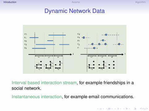
Interval based interaction stream, for example friendships in asocial network.
Instantaneous interaction, for example email communications.
Introduction Axioms Algorithm
Dynamic Network Data
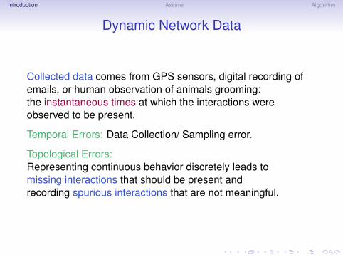
Collected data comes from GPS sensors, digital recording ofemails, or human observation of animals grooming:the instantaneous times at which the interactions wereobserved to be present.
Temporal Errors: Data Collection/ Sampling error.
Topological Errors:Representing continuous behavior discretely leads tomissing interactions that should be present andrecording spurious interactions that are not meaningful.
Introduction Axioms Algorithm
Temporal Scale of Dynamic NetworksDynamic Network
6Temporal Scale of Dynamic Networks
t=1 t=3 t=4 t=5t=2 t=6
Introduction Axioms Algorithm
Temporal Scale of Dynamic NetworksDynamic Network
6Temporal Scale of Dynamic Networks
t=1 t=3 t=4 t=5t=2 t=6
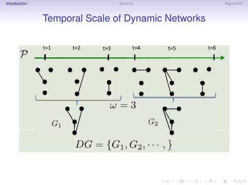
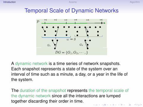
A dynamic network is a time series of network snapshots.Each snapshot represents a state of the system over aninterval of time such as a minute, a day, or a year in the life ofthe system.
The duration of the snapshot represents the temporal scale ofthe dynamic network since all the interactions are lumpedtogether discarding their order in time.
Introduction Axioms Algorithm
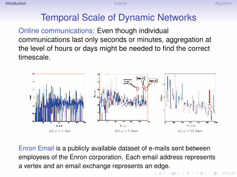
Temporal Scale of Dynamic NetworksOnline communications: Even though individualcommunications last only seconds or minutes, aggregation atthe level of hours or days might be needed to find the correcttimescale.
70
(a) ω = 1 day (b) ω = 5 days (c) ω = 12 days
Figure 14: Network radius time series for the Enron dataset at three levels of aggregation: (a)fine level of aggregation, ω = 1 day, (c) coarse level of aggregation, ω = 12 days, (b) theright level of aggregation, ω = 5 days.
like to achieve when we aggregate at the right scale. We would like to smooth out only the
noise, without affecting the quality of the actual signal (information) in the data.
6.1.3.3 Comparison with Graphscope and FFT Method.
Graphscope analysis on the Enron dataset partitions the time line on intervals that
vary from 2 weeks to 6 weeks, during the eventful period of November 2001-May 2002.
Some of the major events are captured using this partitions. There are however, several
important events that get smoothed out and can not be spotted when analyzing the time
series aggregated at such coarse levels (Figure 18 (a)). Since GraphScope focuses on
variations of graph compression levels, it is the magnitude of change in the graph structure
that drives the time line partitioning. TWIN analyzes the regularity of compression levels
Enron Email is a publicly available dataset of e-mails sent betweenemployees of the Enron corporation. Each email address representsa vertex and an email exchange represents an edge.

Introduction Axioms Algorithm
Temporal Scale of Dynamic Networks70
(a) ω = 1 day (b) ω = 5 days (c) ω = 12 days
Figure 14: Network radius time series for the Enron dataset at three levels of aggregation: (a)fine level of aggregation, ω = 1 day, (c) coarse level of aggregation, ω = 12 days, (b) theright level of aggregation, ω = 5 days.
like to achieve when we aggregate at the right scale. We would like to smooth out only the
noise, without affecting the quality of the actual signal (information) in the data.
6.1.3.3 Comparison with Graphscope and FFT Method.
Graphscope analysis on the Enron dataset partitions the time line on intervals that
vary from 2 weeks to 6 weeks, during the eventful period of November 2001-May 2002.
Some of the major events are captured using this partitions. There are however, several
important events that get smoothed out and can not be spotted when analyzing the time
series aggregated at such coarse levels (Figure 18 (a)). Since GraphScope focuses on
variations of graph compression levels, it is the magnitude of change in the graph structure
that drives the time line partitioning. TWIN analyzes the regularity of compression levels
Enron Email Dataset.Event 1 represents the time when Karl Rove sold off his energystocks,Event 2 represents the unsuccessful attempt of Dynegy to acquire thebankrupt Enron,Event 3 represents the resignation of Enron’s CEO.
Introduction Axioms Algorithm
Temporal Scale of Dynamic Networks
Animal social interactions:
For example, grooming interactions of baboons usually have atemporal scale ranging from seconds to minutes,mother to infant or peer to peer relationships have a scaleextending over years,an individual troop membership, splitting or formation of newtroops extends from years to decades.
Introduction Axioms Algorithm
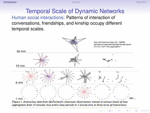
Temporal Scale of Dynamic NetworksHuman social interactions: Patterns of interaction ofconversations, friendships, and kinship occupy differenttemporal scales.
Temporal Scale of Dynamic Networks 8
Effect of Temporal Scale
J. Moody, D. McFarland, and S. Bender-deMoll, ”Dynamic Network Visualization, AJS ’05
Introduction Axioms Algorithm
Temporal Scale of Dynamic Networks71
(a) (b)
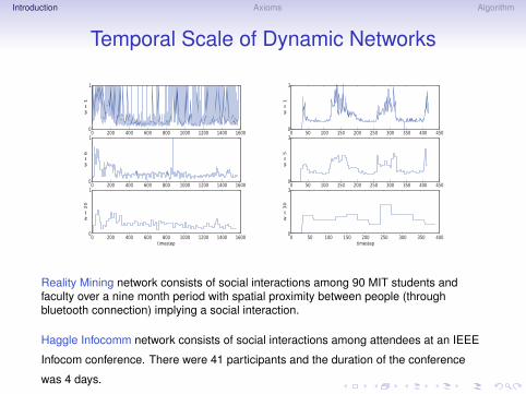
Figure 15: Network density for the Reality Mining dataset (a) and Haggle dataset (b) atthree levels of aggregation: too fine level of aggregation(top picture), the right level ofaggregation (middle picture) and too coarse level of aggregation (bottom picture).
of different metrics on the graph, and therefore, it is the rate of change, not the magnitude,
that will have the most effect in the aggregation.
A nice feature of the Graphscope heuristic is the fact that it generates a non-uniform
partitioning of the time line. The non-uniform partitioning is a more realistic representation
of real-world interaction streams which are commonly characterized by bursty behavior (3;
32). On the other hand, Graphscope determines this partitioning for a fixed aggregation step
and it does not take into account the effect the aggregation step has on the computation of
the compression cost. The estimation of persistent structures leading to the low compression
costs is highly sensitive to the size of aggregation level. TWIN overcomes this dependency
Reality Mining network consists of social interactions among 90 MIT students andfaculty over a nine month period with spatial proximity between people (throughbluetooth connection) implying a social interaction.
Haggle Infocomm network consists of social interactions among attendees at an IEEE
Infocom conference. There were 41 participants and the duration of the conference
was 4 days.

Introduction Axioms Algorithm
Dynamic Network
A temporal stream of edges is a sequence of edges (over afixed vertex set V = {1, . . . ,N}) ordered by their time labels:
E = {(ij , t)|ij ∈ V × V , t ∈ [1, . . . ,T ]}

Introduction Axioms Algorithm
Dynamic Network
Let P be a partition of the timeline [1, . . . ,T ]:
P = p1,p2, . . . ,pk = [t0, t1), [t1, t2), . . . , [tk ,T ]

Introduction Axioms Algorithm
Dynamic Network
Let P be a partition of the timeline [1, . . . ,T ]:
P = p1,p2, . . . ,pk = [t0, t1), [t1, t2), . . . , [tk ,T ]
A dynamic network is a sequence of graphs defined over theedge-stream E and a fixed partition P of [T ]:
〈G1,G2, . . . ,Gi , . . .G|P|〉
with E(Gi) = {(ij , t)|t ∈ pi} andeach Gi is associated with the i th interval pi in P.

Introduction Axioms Algorithm
Dynamic NetworkDynamic Network
6Temporal Scale of Dynamic Networks
t=1 t=3 t=4 t=5t=2 t=6
Introduction Axioms Algorithm
Some Related Work
Empirical Evidence:
Fourier Transform Analysis of Graph parametersClauset, A. and Eagle, N.: Persistence and periodicity in a dynamic proximity network,DIMACS 2007.
Dynamic Network VisualizationMoody, J., McFarland, D., and Bender-deMoll, S.: Dynamic network visualization,American Journal of Sociology, 2005.
Empirical Analysis of Graph ParametersKrings, G., Karsai, M., Bernharsson, S., Blondel, V. D., and Saramaki, J.: Effects of timewindow size and placement on the structure of aggregated networks, CoRR 2012.

Introduction Axioms Algorithm
Some Related Work
Heuristics:
Change detection in interaction streamsSun, J., Faloutsos, C., Papadimitriou, S., and Yu, P. S.: Graphscope: parameter-freemining of large time-evolving graphs, Proc. 13th ACM SIGKDD, 2007.
Community detection in Biological DataBerger-Wolf, T., Tantipathananandh, C., and Kempe, D.: Dynamic CommunityIdentification, In: Link Mining: Models, Algorithms, and Applications, 2010.
Temporal scale detection via linear Graph functionsSulo, R., Berger-Wolf, T., and Grossman, R.: Meaningful selection of temporalresolution for dynamic networks, Proc. 8th Workshop on Mining and Learning withGraphs, 2010.
Introduction Axioms Algorithm
Axioms
What properties should a temporal scale satisfy?
Motivated by axiomatic approaches to “Clustering”:
Impossibility result of Kleinberg 2002.
Quality-based axioms of Ackerman, Ben-David 2008.

Introduction Axioms Algorithm
Axioms
Q, a (quality) function that gives a numerical value to aparticular partition of the timeline and the correspondingdynamic network indicating its “quality”.
What properties must Q satisfy?
Introduction Axioms Algorithm
Axioms
Within Interval Order Invariance:
For an optimal partition, permutations of interactions within thesame interval do not drastically change the quality of thedynamic graph.Some interactions are observed happening in a particular order might be an artifact of
looking at them at too fine of a temporal resolution.

Introduction Axioms Algorithm
Axioms
Across Interval Order Criticality:
For an optimal partition, permutations of edges across differentintervals will change the quality of the partition.
Introduction Axioms Algorithm
Axioms
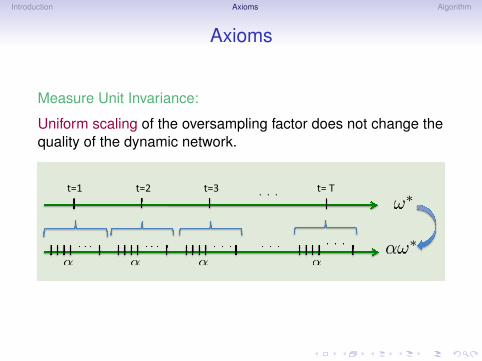
Measure Unit Invariance:
Uniform scaling of the oversampling factor does not change thequality of the dynamic network.
Axiomatic Approach for TSI problem
� Scale Invariance Axiom
. . .. . . . . .. . . . . .
29Temporal Scale of Dynamic Networks
t=1 t=2 t=3 t= T. . .

Introduction Axioms Algorithm
Axioms
Constant Stream:
The constant stream (same set of edges at each moment oftime) has no time scale, the optimal partition is the wholetimeline.

Introduction Axioms Algorithm
Axioms
Stream with no Temporal Scale:
The quality function is the same for any partition of the streamwith no temporal scale, a temporal version of the Erdos-Renyirandom graph (noise).

Introduction Axioms Algorithm
Axioms
Temporal Shift Invariance:
A shift of the time line of a temporal stream, does not drasticallychange the quality of the dynamic network. The optimalpartition of the stream is independent of the time line’s startingpoint.
Introduction Axioms Algorithm
A Persistence Based Approach
Interactions observed fleetingly are often not interesting andthey usually indicate that the data collection process is noisy.
Interactions that persist for a while, truly represent what is moreessential for the underlying system.
What is, then, the “right” temporal scale that can capture thepersistence of structure in time, while smoothing out temporaland topological noise?

Introduction Axioms Algorithm
A Persistence Based Approach
Instead of a global quality function (for the the whole partition ofthe timeline), we will use a local quality function, q, for intervalswithin the partition.
Axioms:
(a) Internal Consistency: q(pi) ≈ q(p∗)
(b) Local Monotonicity: q(pi) ≥ q(pj)
97
[p2] Local Monotonicity: Let p∗ be an interval in an optimal (with respect to q) partition
P∗ of temporal stream Et. Consider two “big enough” subintervals pi, pj ⊆ p∗, such
that |pi|, |pj | > |p∗|/2 and |pi| ≥ |pj | (Figure 29(b)). Then, with high probability, the
bigger subinterval has higher quality:
∀pi, pj ⊆ p∗ s.t. |pi|, |pj | > |p∗|/2, |pi| ≥ |pj |, Pr[q(pi, Eit) ≥ q(pj , E
jt )] ≥ 1− δ
We could think of q1 and q2 as estimations of the rate of change of the edge probability
function. Intuitively, we would expect that during an interval with“optimal persistence”,
the parameters of the edge probability functions stay the same throughout the interval, and
therefore its rate of change is essentially constant. In this sense, we hope both q1 and q2
can capture well at least property p1.
pi
p∗
(a)
pj
pi
pj
pi
p∗
(b)
Figure 29: Illustration of the internal consistency and local monotonicity properties.
Introduction Axioms Algorithm
A Persistence Based Approach
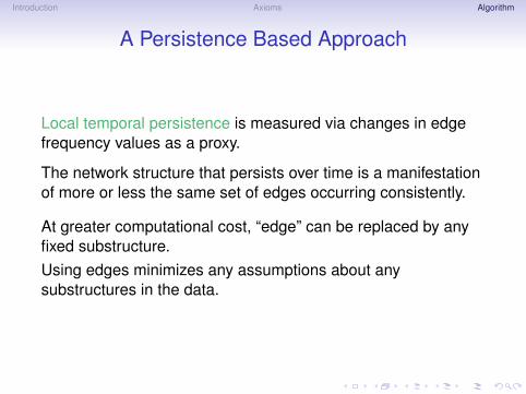
Local temporal persistence is measured via changes in edgefrequency values as a proxy.
The network structure that persists over time is a manifestationof more or less the same set of edges occurring consistently.
At greater computational cost, “edge” can be replaced by anyfixed substructure.Using edges minimizes any assumptions about anysubstructures in the data.

Introduction Axioms Algorithm
A Persistence Based Approach
High persistence of network structure implies persistence ofedge frequency values, but the converse is not necessarily true.
52Temporal Scale of Dynamic Networks
DAPPER Heuristic
� Frequency and Persistence
✔
✗

Introduction Axioms Algorithm
A Persistence Based Approach
freq(p) is the frequency vector (of length |E |) representing thenumber of times each edge occurs in the interval p of thepartition.
fd(pi) is the difference (via an lp norm) between freq(pi andfreq(pi+1), frequency vectors of consecutive intervals - notdisjoint, overlap is controlled by local parameter w .

Introduction Axioms Algorithm
A Persistence Based Approach
Let LM be the set of local maxima:
LM = {i : fd(i) ≥ fd(j), i − r ≤ j ≤ i + r}
where r is the radius for locality.
Introduction Axioms Algorithm
A Persistence Based Approach
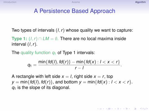
Two types of intervals (l , r) whose quality we want to capture:
Type 1: (l , r) ∩ LM = ∅. There are no local maxima insideinterval (l , r).
The quality function q1 of Type 1 intervals:
q1 =min{fd(l), fd(r)} −min{fd(x) : l < x < r}
r − l.
A rectangle with left side x = l , right side x = r , topy = min{fd(l), fd(r)}, and bottom y = min{fd(x) : l < x < r}.q1 is the slope of its diagonal.

Introduction Axioms Algorithm
A Persistence Based Approach
Type 2: (l , r) ∩ LM 6= ∅. There are local maxima inside interval(l , r).
Let m ∈ LM be the value in (l , r) such that fd(m) is maximized.The quality function q2 of Type 2 intervals:
q2 :=min{fd(l), fd(r)} − fd(m)
r − l.
A rectangle with left side at x = l , right side at x = r , bottom aty = fd(m) and top at y = min{fd(l), fd(r)}.Intuitively, when this box is deeper, we have a better interval.
Introduction Axioms Algorithm
Algorithm
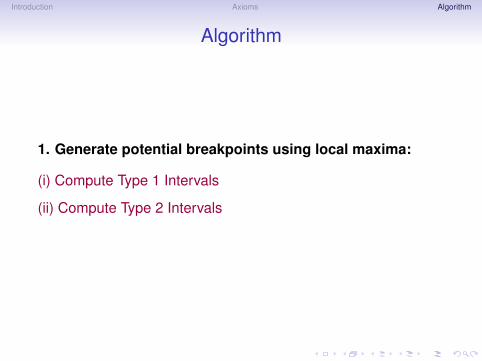
1. Generate potential breakpoints using local maxima:
(i) Compute Type 1 Intervals
(ii) Compute Type 2 Intervals

Introduction Axioms Algorithm
Algorithm
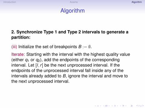
2. Synchronize Type 1 and Type 2 intervals to generate apartition:

Introduction Axioms Algorithm
Algorithm
2. Synchronize Type 1 and Type 2 intervals to generate apartition:
(i) Take the union of Type 1 and Type 2 intervals and theircorresponding q values.

Introduction Axioms Algorithm
Algorithm
2. Synchronize Type 1 and Type 2 intervals to generate apartition:
(ii) Sort the intervals by their q-values in non-increasing order,with ties broken arbitrarily.
Introduction Axioms Algorithm
Algorithm
2. Synchronize Type 1 and Type 2 intervals to generate apartition:
(iii) Initialize the set of breakpoints B := ∅.Iterate: Starting with the interval with the highest quality value(either q1 or q2), add the endpoints of the correspondinginterval. Let [l , r ] be the next unprocessed interval. If theendpoints of the unprocessed interval fall inside any of theintervals already added to B, ignore the interval and move tothe next unprocessed interval.
Introduction Axioms Algorithm
Algorithm
2. Synchronize Type 1 and Type 2 intervals to generate apartition:
(iv) When the procedure quits: if B = {b1, . . . ,bk} withb1 < . . . < bk , then our final answer is the set of intervals[0,b1), [b1,b2), . . . , [bk ,T ].

Introduction Axioms Algorithm
Algorithm91
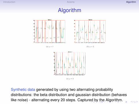
(a) ω = 1 (b) ω = 2
(c) ω = 3
Figure 26: Partitioning of the DynMix stream by the DAPPER heuristic. The red verticallines represent the partitioning points along the time line.
(regions with very low and stable frequency difference values), DAPPER still over-partitions
at ω = 1. This problem seems to be corrected as the value of ω is increased and we notice
that for ω = 4 (40 minute intervals), we see a clear separation between the day and night
frequency patterns (Figure 27(c)). Also, note that some of the finer partitions at this scale,
do indeed correspond to intervals of length 20 minutes, 30 minutes, 50 minutes and about
3-4 hours. The results map consistently to the temporal organization of the conference and
Introduction Axioms Algorithm
Algorithm
91
(a) ω = 1 (b) ω = 2
(c) ω = 3
Figure 26: Partitioning of the DynMix stream by the DAPPER heuristic. The red verticallines represent the partitioning points along the time line.
(regions with very low and stable frequency difference values), DAPPER still over-partitions
at ω = 1. This problem seems to be corrected as the value of ω is increased and we notice
that for ω = 4 (40 minute intervals), we see a clear separation between the day and night
frequency patterns (Figure 27(c)). Also, note that some of the finer partitions at this scale,
do indeed correspond to intervals of length 20 minutes, 30 minutes, 50 minutes and about
3-4 hours. The results map consistently to the temporal organization of the conference and
Synthetic data generated by using two alternating probabilitydistributions: the beta distribution and gaussian distribution (behaveslike noise) - alternating every 20 steps. Captured by the Algorithm.

Introduction Axioms Algorithm
Algorithm
92
in this sense, DAPPER captures the right scale of the underlying dynamics of the Haggle
dataset.
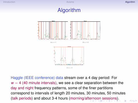
(a) ω = 1 (b) ω = 2
(c) ω = 4
Figure 27: Partitioning of the Haggle stream by the DAPPER heuristic. The red verticallines represent the partitioning points along the time line.
Introduction Axioms Algorithm
Algorithm
92
in this sense, DAPPER captures the right scale of the underlying dynamics of the Haggle
dataset.
(a) ω = 1 (b) ω = 2
(c) ω = 4
Figure 27: Partitioning of the Haggle stream by the DAPPER heuristic. The red verticallines represent the partitioning points along the time line.
Haggle (IEEE conference) data stream over a 4 day period: Forw = 4 (40 minute intervals), we see a clear separation between theday and night frequency patterns, some of the finer partitionscorrespond to intervals of length 20 minutes, 30 minutes, 50 minutes(talk periods) and about 3-4 hours (morning/afternoon sessions).

Introduction Axioms Algorithm
Future Work/ Open Questions
Conjecture: There is no global quality function that satisfies allthe axioms.

Introduction Axioms Algorithm
Future Work/ Open Questions
Conjecture: There is no global quality function that satisfies allthe axioms.
Find a global quality function that captures “many” of theaxioms.

Introduction Axioms Algorithm
Future Work/ Open Questions
Conjecture: There is no global quality function that satisfies allthe axioms.
Find a global quality function that captures “many” of theaxioms.
Show that the solution of our algorithm satisfies “some” of theglobal axioms.
Introduction Axioms Algorithm
Future Work/ Open Questions
Conjecture: There is no global quality function that satisfies allthe axioms.
Find a global quality function that captures “many” of theaxioms.
Show that the solution of our algorithm satisfies “some” of theglobal axioms.
In any algorithm, how can we determine the threshold value ofwindow size (w) beyond which temporal scaling ismeaningless/ useless?
How to determine best-fit subgraph within each interval in orderto minimize topological errors?
New Algorithms. New applications.