1

TEMPORARY PERMIT FOR

DIVERSION AND USE OF WATER

APPLICATION T032564 TEMPORARY PERMIT 21364

Permittee:

Scott Valley Irrigation District PO Box 216

Fort Jones, CA 96032

Summary Report

Prepared by:

2

Helen E. Dahlke, Assistant Professor Dept. of Land, Air and Water Resources, UC Davis

Jim Morris, Director, Scott Valley Irrigation District

With contributions from Preston Harris, Erich Yokel, Gary Black, Gus Tolley, Steve Orloff and Thomas Harter

3

Executive Summary On January 13, 2016 the Scott Valley Irrigation District (SVID) received a temporary permit to appropriate surface water for groundwater recharge and later instream fish and wildlife habitat enhancement between River Mile (RM) 46.7 and RM 21 in the period January 1 to March 31, 2016. The original application proposed to divert up to 5,400 acre-feet (AF) for groundwater recharge on agricultural fields (about 1,400 acres) adjacent to the SVID ditch. Diversion of surface water for groundwater recharge started on February 4th and ceased on March 31, 2016. Based on streamflow estimates at the point of diversion (POD) at RM 46.7, a total of 680 AF were diverted for groundwater recharge while an almost equal amount (675 AF) was diverted for stockwater use. Surface water was recharged on 5 fields. A total of 8 groundwater wells were instrumented with pressure transducers on the east side of the Scott River to monitor changes in the groundwater surface elevation in response to the artificial recharge activities and natural recharge of precipitation. Based on these measurements a clear response was observed in the elevation of the groundwater table: In the immediate vicinity of the recharge site, water levels rose by 4.5 ft in response to the intentional recharge indicating that on-farm recharge resulted in a measurable, temporary increase in groundwater storage leading to later groundwater contribution to streamflow. Since October 1, 2015 and through the period including intentional recharge, the Scott Valley also received a total of 23.75 inches of precipitation. Monitoring of water levels at several locations across the Scott Valley confirmed that precipitation had an overall much larger effect on Scott Valley groundwater storage than the small field-scale recharge events. No changes occurred in landuse or summer irrigation patterns. We used the Scott Valley Integrated Hydrologic Model, a surface water-groundwater model of the Scott Valley, to simulate the diversion and recharge occurring during the experiment as a simulation scenario. Comparison to the base case demonstrates that the recharged water ultimately benefitted streamflows downgradient and downstream from the recharge site during and after the actual diversion.

Of significant concern to growers are potential crop production losses resulting from intentional winter irrigations in alfalfa. From a hydrologic perspective, either increases or decreases in crop production are important as they may be associated with some increases or decreases in consumptive water use for crop production, depending on soils, climate, and irrigation practices. Overall, the alfalfa yield in the three treatment areas showed no discernible difference in yield in response to the winter irrigation. These results suggest that alfalfa is a promising crop for agricultural recharge if grown on suitable, well-draining soils.

Overall, the study can be considered a successful implementation of intentional recharge on agricultural land for groundwater storage and streamflow enhancement with significant amounts of water recharged (relative to the size of agricultural land used), with demonstrable benefits to later streamflow, and considerable landowner support for adoption of these practices.

4

Table of Contents 1 Diversion and streamflow measurements ................................................................................ 8

2 Groundwater recharge and storage ........................................................................................ 12

3 Streamflow enhancement modeling ...................................................................................... 25

4 Flooding tolerance of alfalfa .................................................................................................. 31

4.1 Experimental Setup ........................................................................................................ 31

4.2 Results ............................................................................................................................ 33

4.3 Major findings – Crop study .......................................................................................... 37

5 References ............................................................................................................................. 37

5

Figures Figure 1: Daily average discharge (cfs) at USGS stream gauge near Fort Jones (USGS 11519500) (a) and at the SVID point of diversion (POD) (b). The orange dotted line in (a) indicates the minimum flow requirement of 426 cfs specified in the Scott River Decree. ............ 8 Figure 2: Calculated and measured discharge (cfs) at SVID point of diversion – 2/1 – 4/3/2016. 9 Figure 3: Daily accumulated volume (acre feet) - SVID point of diversion. ............................... 10 Figure 4: Discharge (cfs) at USGS Station (11519500) Scott River near Fort Jones – Data retrieved at http://waterdata.usgs.gov/ca/nwis/uv/?site_no=11519500&PARAmeter_cd=00065,00060 on 5/18/2016. ..................................................................................................................................... 10 Figure 5: Locations of spreading grounds and groundwater and surface water elevation monitoring. POD is the point of diversion, CIMIS 225 is the location of the California Irrigation Management Information System station where meteorological parameters were measured, BL, HA and HR locations are points where water surface elevation was monitored. JM1, JM2, BL3, HR2, and HA3 are also recharge locations. .................................................................................. 13 Figure 6: Locations of fields receiving surface water for groundwater recharge. Note the experimental site instrumented by UC Davis (JM1) and JM2 are not shown on this map (see Figure 33). ..................................................................................................................................... 14 Figure 7: Calculated and measured water surface elevation – HA2. ............................................ 15 Figure 8: Water temperature – HA2. ............................................................................................ 15 Figure 9: Calculated and measured water surface elevation – BL1. ............................................. 17 Figure 10: Water temperature – HA2. .......................................................................................... 17 Figure 11: Calculated and measured water surface elevation –BL3. ............................................ 18 Figure 12: Water temperature – HA2. .......................................................................................... 18 Figure 13: Calculated and measured water surface elevation – BL4. ........................................... 19 Figure 14: Water temperature – HA2. .......................................................................................... 19 Figure 15: Calculated and measured water surface elevation – BL5. ........................................... 20 Figure 16: Water temperature – HA2. .......................................................................................... 20 Figure 17: Calculated and measured water surface elevation – EH Pond. ................................... 21 Figure 18: Water temperature – HA2. .......................................................................................... 22 Figure 19: Calculated and measured water surface elevation – HA3. .......................................... 22 Figure 20: Water temperature – HA2. .......................................................................................... 23 Figure 21: Calculated and measured water surface elevation – HR1. .......................................... 23 Figure 22: Water temperature – HA2. .......................................................................................... 24 Figure 23: Calculated and measured water surface elevation – HR2. .......................................... 25 Figure 24: Water temperature – HA2. .......................................................................................... 25 Figure 25: Recharge locations and recharge rates from on-farm flooding assumed in the SVIHM model............................................................................................................................................. 27 Figure 26: Groundwater elevation at location BL1 for Jan. 1 – May 1, 2016 (left) and the 2016 calendar year for the modeled baseline (black line) vs. recharge scenario (dashed line). ............ 29

6

Figure 27: Groundwater elevation at location BL3 for Jan. 1 – May 1, 2016 (left) and the 2016 calendar year for the modeled baseline (black line) vs. recharge scenario (dashed line). ............ 29 Figure 28: Groundwater elevation at location EH_pond for Jan. 1 – May 1, 2016 (left) and the 2016 calendar year for the modeled baseline (black line) vs. recharge scenario (dashed line). .. 30 Figure 29: Groundwater elevation at locations HA1 and HA2 for Jan. 1 – May 1, 2016 (left) and the 2016 calendar year for the modeled baseline (black line) vs. recharge scenario (dashed line)........................................................................................................................................................ 30 Figure 30: Groundwater elevation at location HA3 for Jan. 1 – May 1, 2016 (left) and the 2016 calendar year for the modeled baseline (black line) vs. recharge scenario (dashed line). ............ 30 Figure 31: Groundwater elevation at location JM1 for Jan. 1 – May 1, 2016 (left) and the 2016 calendar year for the modeled baseline (black line) vs. recharge scenario (dashed line). ............ 31 Figure 32: Comparison of simulated streamflow at USGS Fort Jones stream gauge between the basecase scenario (black line) and the 2016 MAR scenario (blue line) (left panel). MAR diversion rate (orange), the difference in Scott River streamflow due to MAR at the USGS Fort Jones stream gauge, and the relative recovery of loss in streamflow at the Ft. Jones gauge during the February – March MAR diversion as enhanced streamflow after March 31 (black) (right panel)............................................................................................................................................. 31 Figure 33: 15-acre field with 10-year alfalfa stand (JM1). Three different water application rates were tested: continued, high, low and no water (control) application. Numbers indicate individual checks. The yellow star indicates the location of JM2. ............................................... 32 Figure 34: Amount of water diverted for winter recharge (cfs), change in groundwater level below surface (ft) and rainfall (in/day) measured in winter 2014/15 and 2015/16. ..................... 33 Figure 35: Alfalfa yield for 1st (orange, end of May), 2nd cutting (blue, mid-July), and 3rd cutting (green, end of August) vs. average applied winter water (ft) for 2015 and 2016. ............ 35 Figure 36: Winter flood irrigation on the second field on Bryan-Morris ranch. Flow from the valve was estimated at 0.3 cfs. ...................................................................................................... 37 Tables Table 1: Periodic discharge (cfs) measurements performed at the SVID POD for 2016 Groundwater Recharge. .................................................................................................................. 9 Table 2: Daily average discharge (cfs) and daily volume (acre feet) at SVID point of diversion. Daily discharge and daily volume diverted for recharge (column 4 and 5). ................................. 11 Table 3: List of recharge sites and time periods during which surface water was applied for groundwater recharge.................................................................................................................... 12 Table 4: Coordinates of HA2 and SVID Canal water surface elevation. ..................................... 14 Table 5: Coordinates of BL1 – BL5 and SVID Canal & Scott River water surface elevation. .... 16 Table 6: Coordinates of HA3 and EH Pond.................................................................................. 21 Table 7: Total applied winter water (ft) for groundwater recharge for winters of 2014/15 and 2015/16. ........................................................................................................................................ 34

7

Table 8: Harvest data for second alfalfa field on Bryan-Morris ranch. Forage was harvested on June 1, 2016. ................................................................................................................................. 36

8

1 Diversion and streamflow measurements The temporary permit for groundwater recharge was issued by the State Water Resources Control Board (SWRCB) to the Scott Valley Irrigation District (SVID) on January 13, 2016. Shortly after the permit was issued SVID volunteer staff started instrumenting groundwater wells and the SVID point of diversion with hydrologic sensors to measure flow rate at the point of diversion and changes in the depth to the groundwater table near fields that would receive water for groundwater recharge. Diversion of surface water for groundwater recharge began on February 4, 2016 and ended on March 31, 2016. Recharge was extended until April 22, 2016 on the research field described below.

Based on precipitation data from the Western Regional Climate Center (Fort Jones Ranger Station, COOP ID 043182, Elev. 2730 ft a.s.l.) the Scott Valley received a total of 23.75 inches of precipitation in water year (WY) 2015/16. Of that, 5.07 inches fell between February 1 and March 31, 2016. The total annual average precipitation in WY 2015/16 was slightly above the long-term average of 19.5 inches (1935-2012). In response to the large precipitation events, the flow in the Scott River stayed consistently high (above the 1,000 cfs mark) between January and April in 2016. At no time during this 2-months groundwater recharge period did the streamflow at USGS stream gauge in Fort Jones drop below the USFS minimum flow requirement specified in the Scott River Decree (Fig. 1a).

Figure 1: Daily average discharge (cfs) at USGS stream gauge near Fort Jones (USGS 11519500) (a) and at the SVID point of diversion (POD) (b). The orange dotted line in (a) indicates the minimum flow requirement of 426 cfs specified in the Scott River Decree.

9

The discharge measured at the SVID POD during the diversion period for groundwater recharge is shown in Figure 2. Stage measurements (ft) were converted to volume measurements through a stage-discharge relationship. To establish the stage-discharge relationship eight discharge (cfs) measurements were taken with a flow meter at different flow rates as indicated by the blue dots in Figure 2. Table 1 summarized the dates, time and observed discharge measured with the flow meter at SVID POD.

Figure 2: Calculated and measured discharge (cfs) at SVID point of diversion – 2/1 – 4/3/2016.

Table 1: Periodic discharge (cfs) measurements performed at the SVID POD for 2016 Groundwater Recharge.

Between February 1 and April 1, 2016 a total of 1355 AF of surface water were diverted at SVID POD from the Scott River. This total includes the amount of water diverted under the existing SVID stockwater right as well as the water diverted for groundwater recharge under this permit (Figure 3). Surface water demand for livestock is about 7.5 cfs. Stockwater demands was

10

subtracted from the observed SVID POD discharge on days when discharge was greater than 7.5 cfs (Table 2). On days when SVID POD discharge was less than 7.5 cfs it was assumed that the SVID discharge was entirely used for livestock. Diversions in excess of 7.5 cfs totalled 680 acft. Actual groundwater recharge is likely somewhat higher as water demand for livestock is varying on a day-to-day basis based on temperature and animal needs.

Figure 3: Daily accumulated volume (acre feet) - SVID point of diversion.

Figure 4: Discharge (cfs) at USGS Station (11519500) Scott River near Fort Jones – Data retrieved at http://waterdata.usgs.gov/ca/nwis/uv/?site_no=11519500&PARAmeter_cd=00065,00060 on 5/18/2016.

11

Table 2: Daily average discharge (cfs) and daily volume (acre feet) at SVID point of diversion. Daily discharge and daily volume diverted for recharge (column 4 and 5).

12

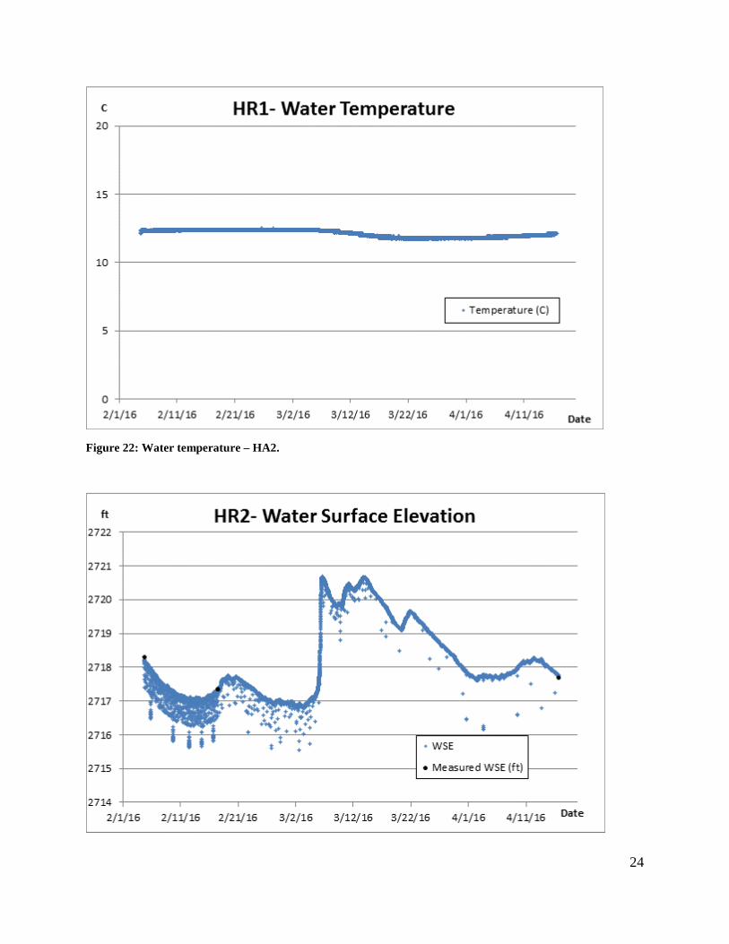
2 Groundwater recharge and storage Groundwater and surface water elevations were documented using water level loggers during the period of February – April 2016 in selected locations within the Scott Valley Irrigation District (SVID). Nine sites were monitored of which eight were groundwater wells (HR1, HR2, HA2, HA3, BL1, BL3, BL4, BL5) (Fig. 5). Seven of the monitored sites’ elevations were documented using a RTK GNSS survey system with a post correction from NGS – OPUS to NAVD 88 computed using GEIOD 12B. Two of the sites elevations were calculated using the previous documented elevation (HR1 & HR2). Water level loggers (Onset U20 and U20L) were placed in the monitored sites. Manual measurements of depth to water from the surveyed reference point were performed. Calculations of the water surface elevation were performed using the continuous data, manual data and surveyed reference point elevation. Water temperature was documented.

Water was diverted onto 5 fields: JM1, JM2, BL3, HR2, and HA3 (Fig. 5 & 6). In addition, a small fraction (0.5 cfs) was turned out from SVID ditch into one of the laterals in Hamlin Gulch. The following table is summarizing the time periods for which water was applied onto each site.

Table 3: List of recharge sites and time periods during which surface water was applied for groundwater recharge.

Site Time period

JM1 2/4/ – 4/1/2016

JM2 2/4/ – 4/1/2016

BL3 2/23 – 2/28 and 3/9 – 3/16/2016

HR2 3/2 – 4/1/2016

HA3 3/12 – 3/22/2016

Most water surface elevations showed an increase in elevation in response to the large precipitation events in mid-February and early March. In some cases, water surface elevations increased by several feet over the winter and spring season followed in some cases (e.g., BL1, BL3) immediate decline in water level elevations. The large influx of surface water into the Scott Valley groundwater aquifer system was also supported by the groundwater temperature data, which in all cases showed a decrease in temperature in response to the influx of colder surface water at the recharge sites.

With exception of the Bryan-Morris ranch, where water level changes could be monitored directly on site, it was not possible to quantify the rise in groundwater storage related to groundwater recharge vs. natural recharge from precipitation. This is in part due to the fact that most monitoring wells were either located at larger distance or upgradient from the research sites, or the monitoring wells were located in an area that received a large influx of surface water from tributaries (gulches) along the east side of Scott Valley. Considering that the winter of

13

2015/16 had above average precipitation, we conclude that the amount of surface water applied for groundwater recharge was too small to be discernible from natural recharge in all but onsite monitoring wells. For future work, we hope to increase the recharge amount, spreading area and duration of surface water applications for groundwater recharge to maximize the benefits for instream flows.

Figure 5: Locations of spreading grounds and groundwater and surface water elevation monitoring. POD is the point of diversion, CIMIS 225 is the location of the California Irrigation Management Information System station where meteorological parameters were measured, BL, HA and HR locations are points where water surface elevation was monitored. JM1, JM2, BL3, HR2, and HA3 are also recharge locations.

JM 1

JM 2

14

Figure 6: Locations of fields receiving surface water for groundwater recharge. Note the experimental site instrumented by UC Davis (JM1) and JM2 are not shown on this map (see Figure 33).

Table 4: Coordinates of HA2 and SVID Canal water surface elevation.

15

Figure 7: Calculated and measured water surface elevation – HA2.

Figure 8: Water temperature – HA2.

16

Table 5: Coordinates of BL1 – BL5 and SVID Canal & Scott River water surface elevation.

17

Figure 9: Calculated and measured water surface elevation – BL1.

Figure 10: Water temperature – HA2.

18

Figure 11: Calculated and measured water surface elevation –BL3.

Figure 12: Water temperature – HA2.

19

Figure 13: Calculated and measured water surface elevation – BL4.

Figure 14: Water temperature – HA2.

20

Figure 15: Calculated and measured water surface elevation – BL5.

Figure 16: Water temperature – HA2.

21

Table 6: Coordinates of HA3 and EH Pond.

Figure 17: Calculated and measured water surface elevation – EH Pond.

22

Figure 18: Water temperature – HA2.

Figure 19: Calculated and measured water surface elevation – HA3.

23

Figure 20: Water temperature – HA2.

Figure 21: Calculated and measured water surface elevation – HR1.

24

Figure 22: Water temperature – HA2.

25

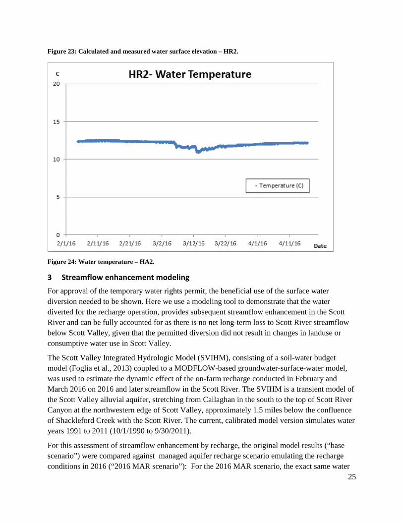
Figure 23: Calculated and measured water surface elevation – HR2.

Figure 24: Water temperature – HA2.

3 Streamflow enhancement modeling For approval of the temporary water rights permit, the beneficial use of the surface water diversion needed to be shown. Here we use a modeling tool to demonstrate that the water diverted for the recharge operation, provides subsequent streamflow enhancement in the Scott River and can be fully accounted for as there is no net long-term loss to Scott River streamflow below Scott Valley, given that the permitted diversion did not result in changes in landuse or consumptive water use in Scott Valley.

The Scott Valley Integrated Hydrologic Model (SVIHM), consisting of a soil-water budget model (Foglia et al., 2013) coupled to a MODFLOW-based groundwater-surface-water model, was used to estimate the dynamic effect of the on-farm recharge conducted in February and March 2016 on 2016 and later streamflow in the Scott River. The SVIHM is a transient model of the Scott Valley alluvial aquifer, stretching from Callaghan in the south to the top of Scott River Canyon at the northwestern edge of Scott Valley, approximately 1.5 miles below the confluence of Shackleford Creek with the Scott River. The current, calibrated model version simulates water years 1991 to 2011 (10/1/1990 to 9/30/2011).

For this assessment of streamflow enhancement by recharge, the original model results (“base scenario”) were compared against managed aquifer recharge scenario emulating the recharge conditions in 2016 (“2016 MAR scenario”): For the 2016 MAR scenario, the exact same water

26

year 1991-2011 simulation was performed as for the base scenario, but with 680 AF of water diverted from the Scott River at the Scott Valley Irrigation District point of diversion (POD) and with 680 AF of water recharged at the fields at which actual recharge was implemented, from February 1, 1998 to March 31, 1998 (59 days). The winter of 1998 was chosen as 1998 and 2016 had approximately similar streamflow conditions during the early part of the year. The simulated rate of surface water diversion for recharge was 5.9 cfs (680 AF over 59 days). Figure 25 shows the recharge locations and approximate recharge amounts considered in the model.

Approximately 70% of the estimated 680 AF of recharge was applied to fields HR2, EH Pond, JM1, JM2 (green fields, Fig. 25) and 30% was applied to fields HA3 and BL3 (pink fields, Fig. 25). Given the area of these fields, this corresponds to managed aquifer recharge rates of 0.0194 m/day and 0.0098 m/day, respectively. These recharge rates are added to the recharge-from-precipitation rates that are used in the base scenario model at these fields. Hydrographs of these locations are shown in figures 26 to 31 show modeled increases in groundwater levels. Figure 32 shows comparisons of streamflow for the base and recharge scenario.

27

Figure 25: Recharge locations and recharge rates from on-farm flooding assumed in the SVIHM model.

During the diversion period, Scott River streamflows continuously exceeded 1,000 cfs. The diversion of 5.9 cfs is less than 1% of the actual (and simulated) streamflow in the Scott River. To illustrate the cumulative effect of the 2016 MAR scenario on downstream streamflow, we therefore focus on demonstrating the differences in streamflow at the USGS Ft. Jones gauge before, during, and after the February 1 to March 31 MAR diversion, relative to the base scenario (Figure 32). In the model, the Scott River outflow point from the simulation domain is considered representative of the location of the USGS Ft. Jones gauging station.

28

Results indicate that, as expected, there are no simulated flow differences at the gauge prior to February 1. Immediately after diversion of 5.9 cfs begins on February 1, streamflow immediately below the POD is reduced by 5.9 cfs (not shown). However, streamflow at the gauge – relative to the base scenario - is reduced by not quite 4 cfs. Throughout February and March, this difference in simulated streamflow at the USGS Ft. Jones gauge decreases to less than 1 cfs, despite the fact that 5.9 cfs continue to be diverted at the POD. After the diversion ends abruptly at the beginning of April, the simulated 2016 MAR scenario streamflow at the USGS Ft. Jones gauge is over 3 cfs higher than in the base scenario. This streamflow enhancement effect continues into the early summer and decreases exponentially with time. Given the pilot scale of the current recharge experiment, designed primarily to test the recharge effects on crops and immediately underlying water levels, the difference in the simulated streamflow during the critical low flow season in August and September is not surprisingly small relative to actual streamflow.

By the end of the year, the simulation predicts that nearly 90% of downstream streamflow losses during February and March will have been recovered as downstream streamflow enhancement during April through December. The remainder of the recovery occurs during the following year (95%) and subsequent years. By 2011 (13 years after the recharge event), the total simulated streamflow recovery of the 680 AF diversion is over 99.5%.

The total decrease in downstream outflow volume during February and March represents less than one-third of the actual diversion amount of 680 AF. Downstream outflow from Scott Valley is buffered from the full diversion effect because groundwater contributions to the stream increase below the diversion point. These increases in groundwater contributions to streamflow are thought to initially be due to the slightly lower streamflows and, hence, slightly lower water levels in the stream. This induces a slight increase in groundwater flow to the Scott River, where it is gaining, and a decrease in Scott River recharge to groundwater, where it is losing. Soon after the beginning of the recharge operation, increasing water levels near the recharge basins, particularly where they are close the Scott River increase the (relative) groundwater outflow to the stream, effectively returning recharge, with some delay, back to the Scott River. This explains the decreasing downstream streamflow losses during February and March.

Given that both, the diversion rate and the differences in streamflow rate are less than 1% of total streamflow, numerical roundoff errors and the coarse simulation time-steps (20 time steps over 2 months) may also introduce some inaccuracies in the exact timing and amount of streamflow difference at the USGS Ft. Jones gauge between the 2016 MAR scenario and the base scenario.

The results from this simulation qualitatively agree with a full scale managed aquifer recharge scenario that was modeled for the Scott Valley Groundwater Advisory Committee. For the full scale MAR scenario (“MAR scenario”) simulation, a winter diversion of 42 cfs was implemented over a full 90 days from January through March (totaling approximately 7500 acre-ft per winter). The diversion rate represents the actual diversion capacity at the POD. In practice, this rate would partially need to also meet existing winter stock water rights on the diversion canal and could not be completely used for MAR.

29

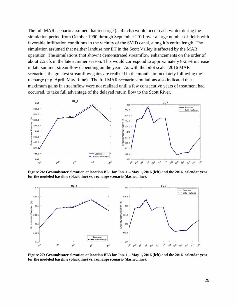
The full MAR scenario assumed that recharge (at 42 cfs) would occur each winter during the simulation period from October 1990 through September 2011 over a large number of fields with favorable infiltration conditions in the vicinity of the SVID canal, along it’s entire length. The simulation assumed that neither landuse nor ET in the Scott Valley is affected by the MAR operation. The simulations (not shown) demonstrated streamflow enhancements on the order of about 2.5 cfs in the late summer season. This would correspond to approximately 8-25% increase in late-summer streamflow depending on the year. As with the pilot scale “2016 MAR scenario”, the greatest streamflow gains are realized in the months immediately following the recharge (e.g. April, May, June). The full MAR scenario simulations also indicated that maximum gains in streamflow were not realized until a few consecutive years of treatment had occurred, to take full advantage of the delayed return flow to the Scott River.

Figure 26: Groundwater elevation at location BL1 for Jan. 1 – May 1, 2016 (left) and the 2016 calendar year for the modeled baseline (black line) vs. recharge scenario (dashed line).

Figure 27: Groundwater elevation at location BL3 for Jan. 1 – May 1, 2016 (left) and the 2016 calendar year for the modeled baseline (black line) vs. recharge scenario (dashed line).

30

Figure 28: Groundwater elevation at location EH_pond for Jan. 1 – May 1, 2016 (left) and the 2016 calendar year for the modeled baseline (black line) vs. recharge scenario (dashed line).

Figure 29: Groundwater elevation at locations HA1 and HA2 for Jan. 1 – May 1, 2016 (left) and the 2016 calendar year for the modeled baseline (black line) vs. recharge scenario (dashed line).

Figure 30: Groundwater elevation at location HA3 for Jan. 1 – May 1, 2016 (left) and the 2016 calendar year for the modeled baseline (black line) vs. recharge scenario (dashed line).

31

Figure 31: Groundwater elevation at location JM1 for Jan. 1 – May 1, 2016 (left) and the 2016 calendar year for the modeled baseline (black line) vs. recharge scenario (dashed line).

Figure 32: Comparison of simulated streamflow at USGS Fort Jones stream gauge between the basecase scenario (black line) and the 2016 MAR scenario (blue line) (left panel). MAR diversion rate (orange), the difference in Scott River streamflow due to MAR at the USGS Fort Jones stream gauge, and the relative recovery of loss in streamflow at the Ft. Jones gauge during the February – March MAR diversion as enhanced streamflow after March 31 (black) (right panel).

4 Flooding tolerance of alfalfa

4.1 Experimental Setup

To assess the tolerance of alfalfa to winter irrigation and to determine how much water can be recharged on a field planted with alfalfa, an on-farm experiment was conducted on a 15-acre alfalfa field in the Scott Valley (10-year stand in 2016) in the winters of 2014/15 and 2015/16. The field is divided into 11 checks, which were grouped into contiguous areas to test the following four water application rates (see Fig. 33):

(1) continuous application: every-day application of water except when water was being applied to other treatments (3.13 acres total area, checks 1-3),

(2) high water application: 3-5 water applications per week (3.97 acres, checks 4-6),

32

(3) low water application: 1-3 water applications per week (4.46 acres, checks 7-9),

(4) control: no winter water application (3.3 acres, checks 10 and 11, received precipitation only).

Figure 33: 15-acre field with 10-year alfalfa stand (JM1). Three different water application rates were tested: continued, high, low and no water (control) application. Numbers indicate individual checks. The yellow star indicates the location of JM2.

The total amount of applied winter water was measured with a doppler flow meter (Greyline Instruments Inc., green triangle, Fig. 33) and changes in groundwater level was recorded with a pressure transducer deployed in a nearby groundwater well (red dot, Fig. 33). Plant physiological parameters (e.g. total biomass, stem and plant count) were determined in each treatment area before and after the recharge events. In 2015 yield was measured during the first and second cutting on May 27, 2015 and July 15, 2015, respectively. In fall of 2015, the alfalfa field was overseeded with orchardgrass. Plant biomass was harvested on May 24, 2016 (1st cutting) and July 20, 2016 (2nd cutting). In 2015 biomass was collected by hand in several randomly chosen quadrats of 5.5 sq. ft. (0.5 m2) in size. The cut biomass was dried at 140°F (60°C) and yield (tons/acre) was reported on a dry matter basis. In 2016 yield was estimated based on the total wet biomass harvested using a flail-type forage harvester from an approximately 25 x 3 sq. ft. section from each of the 11 checks. A small subsample was taken from the cut biomass and dried at 50 degrees C for at least 48 hours to determine the dry matter of the forage. Subsamples were also

1 2 3 4 5 6 7 8 9 10 11

33

collected by hand clipping areas adjacent to the mowed area to determine the relative proportion of alfalfa, orchardgrass and weed biomass present.

4.2 Results

On the 15-acre field 135 AF and 107 AF of water were applied during the winter/spring season of 2015 and 2016, respectively. Table 7 summarizes the amounts of applied winter water for each check and treatment for both years. The recharged surface water in conjunction with natural precipitation falling caused a rise in the groundwater table in a nearby well (red marker, Fig. 33) of approximately 6 feet in 2015 and 4.5 ft in 2016 (Fig. 34). The continuous treatment plot received winter water for 31 and 46 days in 2015 and 2016, respectively. Estimated infiltration rates averaged 0.9 ft of water per day.

Figure 34: Amount of water diverted for winter recharge (cfs), change in groundwater level below surface (ft) and rainfall (in/day) measured in winter 2014/15 and 2015/16.

34

Table 7: Total applied winter water (ft) for groundwater recharge for winters of 2014/15 and 2015/16.

2014-2015 (02/17-04/09/2015) 2015-2016 (02/04-03/21/2016)

Applied winter water (ft) for recharge Applied winter water (ft) for recharge

Treat-ment Check

Check size

(acres) Irrigation

Days Total February March April Irrigation Days Total February March April

Cont

in.

1 0.84 31 32.66 2.72 24.03 5.90 46 13.52 7.09 6.86 0.09

2 1.1 32 26.49 4.00 17.97 4.51 46 10.32 5.43 5.32 0.09

3 1.19 32 24.87 4.22 16.48 4.17 46 9.54 5.03 4.94 0.09

High

4 1.18 6 7.20 2.67 3.70 0.83 20 4.45 2.93 1.95 0.09

5 1.35 6 6.65 2.50 3.48 0.68 20 3.89 2.57 1.75 0.09

6 1.44 7 8.16 3.27 4.06 0.82 21 3.86 2.64 1.66 0.09

Low

7* 1.41 3 5.20 1.05 1.94 2.21 18 12.96 1.16 1.02 11.31

8 1.51 3 4.18 0.90 2.56 0.72 11 1.63 1.09 0.97 0.09

9 1.54 2 3.35 0.89 1.70 0.76 11 1.60 1.07 0.96 0.09

Cont

rol

10 1.46 0 0.00 0.00 0.00 0.00 0 0.53 0.10 0.34 0.09

11 1.86 0 0.00 0.00 0.00 0.00 0 0.53 0.10 0.34 0.09

* This check received an additional 11.3 ft of water in two irrigation events in April 2016.

35

Figure 35: Alfalfa yield for 1st (orange, end of May), 2nd cutting (blue, mid-July), and 3rd cutting (green, end of August) vs. average applied winter water (ft) for 2015 and 2016.

The winter water application of up to 32 ft of water per treatment showed no discernible effect on alfalfa yield except for the 2nd cutting in 2015, which showed a significant decline in alfalfa yield with increasing amount of applied winter water (Fig. 35a). However, despite the significant decline, the yield in the continuous treatment plot was only 0.5 tons/acre lower than the control, indicating that the economic loss for high water application amounts is modest.

In 2016, checks receiving the largest amount of winter water showed a higher yield than the control plots during the 1st and 2nd cutting indicating that winter recharge may lead to increased crop water availability in the deep soil profile offsetting potential irrigation deficits during the growing season.

36

Part of a second field was flooded on the Bryan-Morris ranch with SVID water between February 4 and March 31, 2016. To estimate the effect of the applied water onto alfalfa yield, biomass was harvested with flail-type forage harvester (see method described in section 4.1). Alfalfa yield data summarized in Table 8 shows the yield data for two areas of the field, one that received additional water during the winter (flooded), the other just rainfall (untreated). In agreement with the experimental plot, there was no discernible difference in the yield between the winter irrigated and non-irrigated areas.

Table 8: Harvest data for second alfalfa field on Bryan-Morris ranch. Forage was harvested on June 1, 2016.

Treated (Flooded)

Harvest wt (lbs)

Plot length (ft)

Wet weight (g)

Dry weight (g)

Dry Matter

Yield (tons/acre)

1 18.0 21.1 504.7 137.1 0.27 1.7

2 21.8 22.3 505.1 136.3 0.27 1.9

3 18.2 19.3 449.5 114.2 0.25 1.7

4 18.4 19.1 480.0 126.7 0.26 1.8

Average 19.1

484.8 128.6 0.26 1.8

Untreated

Harvest wt (lbs)

Plot length (ft)

Wet wt (g)

Dry wt (g)

Dry Matter

Yield (tons/acre)

1 19.5 20.7 435.4 125.1 0.29 2.0

2 20.8 21.6 402.7 120.0 0.30 2.1

3 20.9 28.4 438.1 126.4 0.29 1.5

4 17.7 22.5 484.1 142.7 0.29 1.7

Average 19.7

440.1 128.6 0.29 1.8

37

4.3 Major findings – Crop study

• Alfalfa is a promising crop for ag-recharge if grown on suitable, well-draining soils

• Application of 4-28 ft of water in February/March showed no discernible effect on alfalfa yield

• Winter water application for groundwater recharge might increase soil water availability for alfalfa and offset irrigation deficits during the growing season; however, further research will be needed to better understand the detailed relationship between winter recharge management, summer irrigation management, soil type and moisture profile, and their combined effects on yield

• In CA about 300,000 acres of alfalfa are grown on soils suitable for recharge – applying 6 ft of water would result in 1.6 MAF of recharge (if 90% passed root zone)

5 References

Foglia, L., Mcnally, A., Hall, C., Ledesma, L., Hines, R., and Harter, T., 2013, Scott Valley Integrated Hydrologic Model : Data Collection, Analysis, and Water Budget. Final Report North Coast Regional Water Board, SWRCB Contract 09-084-110 and 11-189-110, 101 pp.

Figure 36: Winter flood irrigation on the second field on Bryan-Morris ranch. Flow from the valve was estimated at 0.3 cfs.