tensor classiﬁcation of structure in smoothed particle

MNRAS 457, 2501–2513 (2016) doi:10.1093/mnras/stw103

Tensor classification of structure in smoothed particle hydrodynamicsdensity fields

Duncan Forgan,1‹ Ian Bonnell,1 William Lucas1 and Ken Rice2

1Scottish Universities Physics Alliance (SUPA), School of Physics and Astronomy, University of St Andrews, North Haugh, St Andrews KY16 9SS, UK2SUPA, Institute for Astronomy, University of Edinburgh, Blackford Hill, Edinburgh EH9 3HJ, UK

Accepted 2016 January 11. Received 2015 December 17; in original form 2015 September 29

ABSTRACTAs hydrodynamic simulations increase in scale and resolution, identifying structures with non-trivial geometries or regions of general interest becomes increasingly challenging. There is agrowing need for algorithms that identify a variety of different features in a simulation withoutrequiring a ‘by eye’ search. We present tensor classification as such a technique for smoothedparticle hydrodynamics (SPH). These methods have already been used to great effect in N-Bodycosmological simulations, which require smoothing defined as an input free parameter. Weshow that tensor classification successfully identifies a wide range of structures in SPH densityfields using its native smoothing, removing a free parameter from the analysis and preventingthe need for tessellation of the density field, as required by some classification algorithms.As examples, we show that tensor classification using the tidal tensor and the velocity sheartensor successfully identifies filaments, shells and sheet structures in giant molecular cloudsimulations, as well as spiral arms in discs. The relationship between structures identifiedusing different tensors illustrates how different forces compete and co-operate to produce theobserved density field. We therefore advocate the use of multiple tensors to classify structurein SPH simulations, to shed light on the interplay of multiple physical processes.

Key words: methods: numerical – stars: formation – ISM: kinematics and dynamics.

1 IN T RO D U C T I O N

Numerical simulations allow astrophysicists to study and cataloguephysical processes on spatial and temporal scales inaccessible toobservations. Flows of matter, energy and angular momentum pro-duce a variety of structures, some of which are simple to detect ‘byeye’, for example spiral arms in astrophysical discs (e.g. Forganet al. 2011; Dipierro et al. 2015), filaments of turbulent gas in gi-ant molecular clouds (GMCs; Klessen & Burkert 2000; Krumholz,Klein & McKee 2011; Bonnell, Dobbs & Smith 2013) or the net-work of dark matter that constitutes the Cosmic Web (e.g. Hahnet al. 2007).

However, ‘by eye’ approaches are unsuitable for determiningthe status of fluid elements on the periphery of a structure – doessuch a simulation element ‘belong’ to a filament or not? Also,incorporating humans directly into any computational algorithm istime-inefficient. For very large simulations, it is increasingly crucialthat any structures produced can be described quickly and reliably.Structure identification is important not only for comparing withobservational data, but also to understand the mechanisms that drivestructure formation, such as self-gravity, turbulence and shocks.

�E-mail: [email protected]

Particle-based simulations have been particularly successful incomputational astrophysics, and structure identification has longbeen a consideration for simulators in this area. N-Body calcula-tions of structure growth in the early Universe have led to usefultopological classifications of the dark matter distribution (Hahnet al. 2007; Forero-Romero et al. 2009; Sousbie 2011; Hoffmanet al. 2012; Libeskind et al. 2013) as well as identification of darkmatter haloes using halo-finding algorithms such as the friends-of-friends (FoF) algorithm, which has many versions and guises(Davis et al. 1985; Knollmann & Knebe 2009 and referencestherein).

In other astrophysical regimes, such as star and planet formation,the local dark matter distribution is less relevant. In these circum-stances baryonic physics, especially hydrodynamics, dominates, butparticle-based simulation is still a commonly used tool, and the needfor structure identification remains. Smoothed particle hydrody-namics (SPH) is a Lagrangian particle simulation technique, whichapproximates a fluid by a distribution of particles. Detailed reviewsof its governing algorithms can be found in Monaghan (1992, 2005)and Price (2012), but for completeness we will state its fundamen-tals here. Each particle is assigned a mass mi, position r i , velocityvi and internal energy ui, and a smoothing length, hi. From this, theproperties of the fluid at any location are derived via interpolationof the particle’s properties, applying a smoothing kernel W to each

C© 2016 The AuthorsPublished by Oxford University Press on behalf of the Royal Astronomical Society

at University of St A

ndrews on June 8, 2016

http://mnras.oxfordjournals.org/

Dow

nloaded from

mailto:[email protected]


2502 D. Forgan et al.

contribution. For example, the local volume density at a location rcan be determined via

ρ(r) =N∑

i=1

miW (|r − r i | , h), (1)

where N represents the number of particles contributing to thesum. Smoothing kernels typically have compact support, and henceare zero at separations greater than 2h. N reduces to the num-ber of ‘nearest neighbours’ that reside within 2h of the parti-cle. This density estimate – along with a suitable definition forthe system Lagrangian/Hamiltonian and application of the Euler–Lagrange/Hamilton’s equations – is sufficient to derive equationsof motion for the entire system, and (with appropriate measurestaken for treatment of shocks and mixing) can simulate fluids inany geometric configuration. Indeed, it has been this ability to dealwith a wide variety of geometries that has made SPH such a populartool in astrophysics, as well as in many other fields of research.

But how should SPH users attempt to classify structure in theirsimulations? Some approaches have the benefit of simplicity, forexample identifying contiguous regions using a density cut has beeneffective in use cases such as finding GMCs in SPH simulations ofgalactic discs (e.g. Dobbs, Pringle & Duarte-Cabral 2014b). Anobvious counter-argument to such approaches is what justifies thevalue of the density cut used. Depending on the system geometry,this value can be motivated by observational constraints, or evenanalytically derived, but in general this may not be the case.

Several algorithms use the linked lists of SPH neighbours, in avein quite similar to FoF algorithms. The CLUMPFIND algorithm,originally developed for imaging purposes (Williams, de Geus &Blitz 1994), identifies separate objects in a simulation according toglobal maxima in density, or global minima in the gravitational po-tential (Klessen & Burkert 2000). Given an appropriate prescriptionfor dealing with objects that touch or overlap in terms of particlepopulation, clumpfind techniques have been useful for identifyingfragments both in GMCs (Smith, Clark & Bonnell 2009) and also indiscs (Hall et al, in preparation). Also of note is the use of minimumspanning trees in hybrid SPH/N-Body calculations (Maschbergeret al. 2010; Kruijssen et al. 2012). However, this technique gener-ally detects structure in the N-Body particles rather than the gas. Fi-nally, we must mention the DisPerSE algorithm, which uses Morsetheory to classify structure using the Delaunay triangulation of dis-crete data (Sousbie 2011). This has proven to be extremely effectivein classifying structures both in numerical simulations (e.g. Smith,Glover & Klessen 2014) and in observational data (e.g. Arzouma-nian et al. 2011) but its use in SPH would require tessellation of thedensity field, an extra layer of assumptions which is preferentiallyavoided.

In this paper, we demonstrate the simplicity and power of usingtensor classification methods on pure SPH data. Originally con-ceived and applied to pure N-Body simulations of the cosmic Web,1

we show that these methods can be applied to pure SPH simula-tions, with the advantage of fewer free parameters. Judicious useof tensor eigenvalues and eigenvectors cannot only identify whichparticles belong to a given structure, but also the orientation of thatstructure with respect to its environment. Classifying via multipletensors allows finer structures to be elucidated, and gives insightinto how various physical forces interact to produce the underlyingstructures seen.

1 This technique has both numerical and observational applications, cf. Guo,Tempel & Libeskind (2015)’s study of the distribution of galaxies.

We structure this paper as follows: in Section 2 we describe thetwo tensors we use to classify SPH structures; in Section 3 we testtheir ability to classify analytically soluble structures; in Section 4we display some of the many applications of these techniques, andin Sections 5 and 6 we discuss and summarize the work.

2 M E T H O D S

2.1 The tidal tensor

The tidal tensor Tij is simply the Hessian of the gravitational poten-tial, φ. In Cartesian co-ordinates {xi}:

Tij = ∂2φ

∂xi∂xj

. (2)

Note that φ is the standard gravitational potential, which solves thecanonical Poisson equation:

∇2φ = 4πGρ, (3)

rather than the pseudo-potential commonly used in cosmologicalsimulations to solve for the matter overdensity. Strictly, Tij as definedabove is the deformation tensor, as the tidal tensor refers to thetraceless component of the Hessian. These labels are commonlyinterchanged in the context of structure identification (Hahn et al.2007; Forero-Romero et al. 2009). We refer to it as the tidal tensorto be clear as to its differences from the velocity shear tensor, whichwe describe in the next section. We utilize the dimensionless formof this tensor:

Tij = ∂2φ

∂xi∂xj

h2

|φ| . (4)

We elect a normalization based on smoothing length as derivativesare computed on the smoothing kernel, and are hence resolution-dependent. In its simplest form:

∇F (r) =N∑

i=1

Fimi

ρi

∇W (|r − r i | , h). (5)

As a result, this places resolution limits on the gradients resolvableby SPH simulations. In the weak field limit, we expect derivativesto follow

∂F

∂xi∂xj

∼ F

h2, (6)

and hence corresponding tensor eigenvalues will be of that order.Our normalization is therefore a depiction of the strength of themeasured gradients in potential at the local simulation resolution,which will become useful later.

2.2 The velocity shear tensor

The velocity shear tensor, �ij, is

�ij = −1

2

(∂vi

∂xj

+ ∂vj

∂xi

). (7)

The astute will note this is equivalent to the strain rate tensor, whichmeasures how the mean velocity in the medium changes betweentwo (infinitesimally) separate locations. The negative sign indicatesthat we are interested in compression of the medium. When used incosmological comoving co-ordinates, it is customary to make thistensor dimensionless by adding in a factor of 1/H0, where H0 is

MNRAS 457, 2501–2513 (2016)




Dow

nloaded from


Classifying structures in SPH 2503

the Hubble constant (Hoffman et al. 2012). As with the tidal tensorabove, we make � dimensionless using the local smoothing length:

�ij = −1

2

(∂vi

∂xj

+ ∂vj

∂xi

)h

|v| . (8)

Again, we adopt an h-dependent normalization due to the h-dependence of the derivative.

2.3 Tensor classification

In all cases, the classification of tensors is algorithmically identical.First, the tensor’s eigenvalues λi and their corresponding eigenvec-tors ni are computed:

T nj = λj nj . (9)

We label the eigenvalues such that λ1 ≥ λ2 ≥ λ3. The tensors usedin this work are real and symmetric, and hence their eigenvaluesare always real. Both tensors assume that the fields being investi-gated (potential, velocity) are smooth and continuous, so that thederivatives are always defined. In N-Body calculations, this meansthe fields must first be smoothed, with the smoothing scale Rs a freeparameter. SPH simulations enjoy the advantage of being alreadyadaptively smoothed according to the local smoothing length h. Ourcalculations henceforth do not require any extra smoothing, and byextension they do not need the above free parameter.

In the case of the tidal tensor, we can now appeal to Zeldovichtheory (Zel’dovich 1970) to motivate our classification. By consid-ering a test particle in orbit around a local extremum in the potential(∇φ = 0), we can linearize its equation of motion to

xi = −Tij xj . (10)

We neglect pressure forces and other terms in this equation ofmotion for the purposes of this illustration. As we can select anappropriate basis such that Tij is diagonal, the linear motion of theparticle is governed by the sign of the eigenvalues. If none of theeigenvalues are positive, then the orbit cannot be stable under anyconfiguration. If all the eigenvalues are positive, the orbit is stableunder all configurations. If one or two eigenvalues are positive, thensome configurations are stable and some are not. More rigorously,the number of positive eigenvalues E describes the dimension ofthe local stable manifold. We should therefore expect tidal tensorclassifications to be effective in regions where pressure gradientsare weak compared to potential gradients.

In a cosmological context, the above argument can also be madefor the velocity shear tensor, as the velocity field and gravitationalfields are close to identical in this limit in the linear regime, up toa scaling dependent on cosmological parameters (Hoffman et al.2012). We are not always at the liberty of making this argument, butwe can state that calculating E for �ij allows us to diagnose the di-mension of the local flow at that instant, albeit with no indication asto whether the configuration is dynamically stable or gravitationallybound.

If E can be calculated for our tensor of choice, we can then makethe following classification:

(i) E = 0 → ‘void’ (0D manifold)(ii) E = 1 → ‘sheet’ (1D manifold)(iii) E = 2 → ‘filament’ (2D manifold)(iv) E = 3 → ‘cluster’ (3D manifold)

In simple terms, E is equivalent to the number of dimensions thelocal medium is being ‘squeezed’ in. Sheets are produced by squeez-ing along one axis, filaments along two axes, clusters along three.

Classification via T is dynamical, and indicates the manifold di-mension of a collapsing region. Classification via � is kinematic,and indicates the manifold dimension of a flow that can either begravitationally bound or unbound.

We have further information to glean from the tensor, in the formof the corresponding eigenvectors. The single positive eigenvalue ofa sheet (λ1) has a corresponding eigenvector (n1) which is parallel tothe normal of the sheet. The single negative eigenvalue of a filament(λ3) has a corresponding eigenvector (n3) which is parallel to theflow direction of the filament. This data now allows us to comparealignments of sheets and filaments to the local environment.

However, we should be cognisant of the dangers of attemptingto discriminate between structure using small, non-zero values ofquantities in numerical simulations. Forero-Romero et al. (2009)give an example of attempting to classify void particles at the in-terface between a void and a sheet region (for example). Accord-ing to the above algorithm, a particle with a single (but infinitesi-mally small) positive eigenvalue will be classified as a sheet. Thisis equivalent to suggesting that in the region of that particle, thelocal medium will collapse into a 1D manifold with a symmetryaxis given by the particle’s n1 eigenvector. In practice, the collapsetime-scale implied by such a small eigenvalue is so long that it isunlikely to occur in the simulation, given the other local time-scalesat play. Forero-Romero et al. (2009) claim that this explains therelatively low proportion of voids found by Hahn et al. (2007) whenusing the positive/negative eigenvalue criterion detailed above.

A solution to this is to instead define E as the number of eigen-values that exceed some threshold value λT. Use of λT allows us toameliorate not only this issue of floating point accuracy, but generalissues that might arise from using this algorithm on SPH densityfields, such as particle disorder and poor resolution in regions oflow particle number.

This threshold parameter λT is the only free parameter in ourclassification scheme. In some simple cases, the value of the thresh-old parameter can be estimated from analytic considerations of theabove collapse time-scale (see appendix A of Forero-Romero et al.2009 and also Alonso, Eardley & Peacock 2015). In the case ofthis work, we investigate the behaviour of the classification as λT

is varied. Thanks to our use of the local smoothing scale in thenormalization of both tensors, λT is now a local threshold, and asa result we find a common property of structure classification as afunction of λT. As we shall see throughout, provided that λT � 1,structures are well resolved. This puts SPH at a distinct advantage topure N-Body simulations, which often rely on multiscale smoothingapproaches to ensure appropriate structure resolution using a globalthreshold (e.g. Hoffman et al. 2012).

3 TESTS

We now consider some simple test cases for both tensors. These testcases have analytic solutions, and therefore we can compare themdirectly to simulation data. Throughout this paper, SPH simulationsare run using the SPHNG code (Bate, Bonnell & Price 1995), usinga variety of prescriptions for the gas equation of state and radiativetransfer, which we will discuss where appropriate.

3.1 The tidal tensor of a uniform density sphere

Consider a sphere, with radius R and uniform density ρ0, embeddedin a vacuum (ρ(r) = 0 for r > R).

MNRAS 457, 2501–2513 (2016)




Dow

nloaded from



Figure 1. The uniform sphere test of the tidal tensor. The fraction of total particles in each class is plotted as a function of the threshold parameter, λT for(left) Case 1, an unrelaxed, noisy particle distribution, and (right) Case 2, a lattice-based particle distribution.

3.1.1 Analytic solution

The potential for this system is spherically symmetric, and hence

φ(r) = φ(r) = −4πG

(∫ r

0ρ(r ′)r ′2dr ′ +

∫ ∞

r

ρ(r ′)r ′dr ′)

. (11)

This integral has the solution:

φ(r) ={ −GM

2R2 (3R2 − r2) r ≤ R

−GMr

r > R. (12)

Where we have substituted for the total mass of the sphere:M = 4/3πGρ0R

3. As the problem is spherically symmetric, wecan use the greatly simplified expression for Tij in spherical polarcoordinates:

Tij = diag

[∂2φ

∂r2,

1

r

∂φ

∂r,

1

r

∂φ

∂r

]. (13)

In the case r ≤ R:

Tij = GM

R3δij . (14)

All the eigenvalues are equal, and positive. Therefore at any locationinside R, the tidal tensor possesses an E = 3, and that locationwill hence be classified as a cluster. This is relatively intuitive– particles inside the sphere experience gravitational forces in allthree dimensions. As r is increased beyond R, the gravitational forcebecomes preferentially directed back towards the sphere, and theparticles are ‘aware’ of the two dimensional nature of the sphere’ssurface. The tidal tensor takes the form:

Tij = GM

r3diag[−2, 1, 1]. (15)

In this case, E = 2 and this region is classified as a filament. Asr → ∞, the force tends to zero, as does eigenvalues of the tensor.As a result, E → 0 and the classification tends towards void status.

3.1.2 SPH results

On the one hand, this test is equivalent to testing the ability of SPHparticles to resolve a surface. On the other hand, this tests the abilityof SPH particles to simulate a uniform density object.

We conduct this test using two sets of SPH initial conditions.In the first, 500 000 particles are placed randomly in an unrelaxeddistribution, resulting in relatively significant particle disorder; inthe second, 300 000 particles are distributed on a lattice with equalseparations. These two cases represent to some degree the best andworst case scenarios in SPH simulations. These snapshots are notevolved – we are interested merely in the classification of the SPHparticles at this given instant. Over the course of a simulation, SPHparticles will arrange themselves to minimize disorder in the system(Monaghan 2005; Price 2012), resulting in conditions belongingsomewhere in between the cases we study here.2

A successful test will identify almost all SPH particles as clus-ters, with a small handful identified as filaments depending on thesimulation’s ability to resolve the spherical surface. Fig. 1 showsthe resulting classifications for both snapshots as a function of thethreshold value, λT. In both cases, we can see that λT must bekept sufficiently small for the classification to be functional: onceλT is larger than the mean eigenvalue, all particles are classed asvoids. Below a critical value of λT ∼ 1, the classification systemis attempting to probe the sub-h limit. In the case of the tidal ten-sor, the potential in the sub-h limit is kernel-smoothed, and hencethe fractions of particles in each class converges to a fixed value.The scaling of the tensor (and subsequently its eigenvalues) by thelocal smoothing length ensures that the critical value of λT is in-dependent of resolution. We confirm this by running both casesagain at lower resolution (100 000 particles), with similar results(Fig. 2).

The unrelaxed snapshot (Case 1) shows the danger of particle dis-order for this classification system. The sphere’s inhomogeneitiesensure that many particles are classified as filaments or sheets ratherthan clusters. This is not merely a surface feature problem, as fil-ament and sheet particles reside at all distances from the centre ofthe sphere (left-hand panel of Fig. 3).

In the lattice snapshot (Case 2), the lack of disorder in the sys-tem allows the tidal tensor to correctly identify over 90 per cent of

2 Note that this ‘intrinsic re-meshing’ will only occur for specific formula-tions of SPH – in effect, whether one derives the SPH equations from theLagrangian or from the Hamiltonian. As a result, most SPH codes select thelatter, as it preserves intrinsic re-meshing. Price (2012)’s discussion of thisis excellent, and hence we will not repeat it here.

MNRAS 457, 2501–2513 (2016)




Dow

nloaded from



Figure 2. As Fig. 1, but with a lower particle number (100 000). This demonstrates that the appropriate threshold to adopt is λT < <1, and that this is resolutionindependent.

Figure 3. The distribution of particles classified as filaments in the higher resolution simulations of Case 1 (left) and case 2 (right), for a threshold parameterof λT = 10−6. The above figures show a cross-section of each simulation, centred on z = 0 with a thickness of 100.

the particles as cluster objects. The relatively low resolution of thesphere’s surface (with thickness ∼h) results in filament identifica-tions for some 8 per cent of particles (right-hand panel Fig. 3).

What should we conclude from this test? A well-ordered particledistribution can pass this test with ease, but noisy distributionscannot. We should therefore consider our particle classificationscarefully, and apply this technique to systems where we can beconfident that any residual noise from initial conditions has beenwell dissipated in the subsequent evolution of the simulation.

3.2 The velocity shear tensor for a radially expanding shell

Consider a radially expanding shell of gas at uniform density withvelocity v1, into a medium with velocity v0 � v1. The velocitygradient is entirely determined by the radial velocity,

∇v = ∂vr

∂rr, (16)

and all other velocity components are zero.

3.2.1 Analytic solution

To obtain this solution, we should rewrite the velocity shear tensorin spherical polar co-ordinates. This gives a quite unwieldy generalexpression, but mercifully when we apply our constraints:

vθ = vφ = ∂v

∂θ= ∂v

∂φ= 0, (17)

the tensor becomes diagonal:

�ij = diag

[−∂vr

∂r, −vr

r, −vr

r

]. (18)

As the radial velocity is positive, and the velocity gradient is nega-tive, this gives E = 1, and therefore the expanding shell is classifiedas a sheet. Outside of the expanding shell, the velocity gradient iszero, and hence E = 0, resulting in a void classification.

3.2.2 SPH results

To test this solution, we begin with a cube of 500 000 particles, ofside L = 1000. Particles with a radius R from the centre of the cubeare assigned a radial velocity v1, and particles outside of this radius

MNRAS 457, 2501–2513 (2016)




Dow

nloaded from



are assigned a radial velocity v0 = 0.8v1. We select a non-zerovalue for v0 to demonstrate the tensor classification algorithm istruly Lagrangian.

Note that our setup is not an expanding shell, but an expand-ing sphere. In the above analytic solution, we should only expectparticles that sense a non-zero velocity gradient locally, i.e. thoseparticles on the boundary between the sphere and the surroundingmedium, to be classified as sheet particles. Inside and outside thesphere, we should expect zero velocity gradients, and hence weshould obtain void classifications for those particles.

Again, we run two tests of this case. In the first, we generate anoisy cube of particles by placing them randomly in Cartesian co-ordinates, and in the second we generate a cubic lattice. Particlesinside a radius of R = 500 from the centre are assigned a radialvelocity vr = v1 = 10, and all other particles are assigned a radialvelocity v0 = 8.

Fig. 4 shows how the global classification of particles varies forboth cases as the eigenvalue threshold λT is increased. In both cases,at appropriate values of λT < 1, the majority of particles are iden-tified as sheets and voids. In the random case (left-hand panel of

Fig. 4), particle noise results in an excess of sheet classifications,even at low λT. In the lattice case, there is no particle noise, andhence there are no erroneous classifications of clusters and fila-ments at any λT. As before, we demonstrate that the λT conditionis resolution independent by repeating the test at lower resolution(Fig. 5).

Fig. 6 shows the distribution of sheet particles (top row) and voidparticles (bottom row) for the random and lattice configurations(left and right, respectively). In both cases, the tensor classificationidentifies the surface of the expanding shell, which has a thicknessof order the local smoothing length, as is evidence by the void clas-sifications. Also, both cases show that particles inside the sphere,more than a smoothing length from the velocity change at R = 500,are classified as voids. However, in Case 1, substantial particle noiseensures that the velocity flow inside and outside the sphere is notprecisely uniform, resulting in a number of erroneous sheet classifi-cations outside of the shell, due to small fluctuations in the velocitygradient. In Case 2, no such problem arises, and the classificationis essentially perfect, even capturing the sheet nature of particles atthe boundary of the cube.

Figure 4. The expanding sphere test of the velocity shear tensor. The fraction of total particles in each class is plotted as a function of the threshold parameter,λT for (left) Case 1, an unrelaxed, noisy particle distribution, and (right) Case 2, a lattice-based particle distribution.

Figure 5. As Fig. 4, but with a lower particle number (100 000). Again, this demonstrates that the appropriate threshold to adopt is λT � 1, and that this isresolution independent.

MNRAS 457, 2501–2513 (2016)




Dow

nloaded from



Figure 6. The distribution of particles by class in Case 1 (left) and Case 2 (right), for a threshold parameter of λT = 10−6. The top plots show particlesclassified as sheets, and the bottom row particles classified as voids.

4 A PPLICATIONS

4.1 Spiral structure in discs

Very young protostellar discs are thought to undergo a briefself-gravitating phase. During this epoch, the Toomre parameter(Toomre 1964):

Q = cs

πG�� 1.5, (19)

where cs, and � are the local sound speed, angular velocity andsurface density, respectively. As a result, non-axisymmetric insta-bilities can grow in the disc (Durisen et al. 2007). These manifest asspiral density waves, with the number of spirals and their propertiesbeing largely determined by the nature of how angular momentumis transported (Forgan et al. 2011).

In extreme circumstances, cool, extended self-gravitating discscan fragment into bound objects (see e.g. Rice, Lodato & Armitage2005). While the precise conditions for fragmentation are the sub-ject of debate (Forgan & Rice 2011; Lodato & Clarke 2011; Meru& Bate 2011; Rice et al. 2014; Young & Clarke 2015), once theseconditions are met fragmentation tends to begin in the spiral arms

themselves, where the local density is significantly higher than themean at that radius. Even when fragmentation does not occur, thesespiral structures are the agents of angular momentum redistribu-tion (and consequently mass accretion) in the disc. It has also beenshown that spiral density waves are capable of accumulating dustvia gas drag, and enhancing grain growth, a result with obviousimplications for subsequent planet formation via core accretion(Rice et al. 2004; Clarke & Lodato 2009; Dipierro et al. 2015).Therefore, an important task for simulators of self-gravitatingdiscs is to understand the growth and evolution of these spiralarms.

Our tensor classification methods can be used to great effecthere. The top-left panel of Fig. 7 shows an SPH simulation of aself-gravitating protostellar disc, which has settled into a quasi-steady state. The star mass is 1 M�, and the disc mass is 0.25 M�.Radiative transfer is approximated using the hybrid formalism ofForgan et al. (2009). The disc is isolated, i.e. it does not accrete froman envelope, and is sufficiently compact to avoid fragmentation.Generation of spiral structures, which produces weak shock heating,is balanced by radiative cooling, resulting in a self-regulated statewhere Q is close to the instability value.

MNRAS 457, 2501–2513 (2016)




Dow

nloaded from



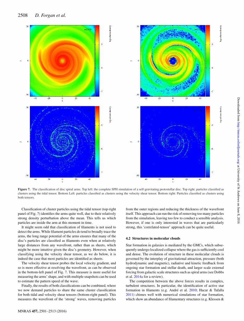
Figure 7. The classification of disc spiral arms. Top left: the complete SPH simulation of a self-gravitating protostellar disc. Top right: particles classified asclusters using the tidal tensor. Bottom Left: particles classified as clusters using the velocity shear tensor. Bottom right: Particles classified as clusters usingboth tensors.

Classification of cluster particles using the tidal tensor (top-rightpanel of Fig. 7) identifies the arms quite well, due to their relativelystrong density perturbation above the mean. This tells us whichparticles are inside the arm at this moment in time.

It might seem odd that classification of filaments is not used todetect the arms. While filament particles do tend to broadly trace thearms, the long range potential of the arms ensures that many of thedisc’s particles are classified as filaments even when at relativelylarge distances from any wavefront, rather than as sheets, whichmight be more intuitive given the disc’s geometry. However, whenclassifying using the velocity shear tensor, as we do below, it isindeed the case that most particles are identified as sheets.

The velocity shear tensor probes the local velocity gradient, andso is more effective at resolving the wavefront, as can be observedin the bottom-left panel of Fig. 7. This measure is more useful formeasuring the arms’ shape, and with multiple snapshots can be usedto estimate the pattern speed of the wave.

Finally, the results of both classifications can be combined, wherewe now demand particles to share the same cluster classificationfor both tidal and velocity shear tensors (bottom-right panel). Thismeasures the wavefront of the ‘strong’ waves, removing particles

from the outer regions and reducing the thickness of the wavefrontitself. This approach can run the risk of removing too many particlesfrom the simulation, leaving too few to conduct a sensible analysis.However, if one is only interested in waves that are particularlystrong, this ‘correlated-tensor’ approach can be quite useful.

4.2 Structures in molecular clouds

Star formation in galaxies is mediated by the GMCs, which subse-quently undergo localized collapse where the gas is sufficiently cooland dense. The evolution of structure in these molecular clouds isgoverned by the interplay of gravitational attraction, pressure (bothhydrodynamic and magnetic), radiative and kinetic feedback fromongoing star formation and stellar death, and larger scale externalforcing from galactic scale structures such as spiral arms (see Dobbset al. 2014a for a review).

The competition between the above forces results in complex,turbulent structures. In particular, the identification of active starformation in filaments (e.g. Andre et al. 2010; Hacar & Tafalla2011) chimes well with numerical simulations of star formation,which show an abundance of filamentary structures (e.g. Klessen &

MNRAS 457, 2501–2513 (2016)




Dow

nloaded from



Figure 8. Particle classifications in the SPH simulation (using the tidal tensor) without a supernova explosion. Top left: the complete SPH simulation. Topright: particles classified as clusters. Bottom left: particles classified as filaments. Bottom right: particles classified as sheets.

Burkert 2000; Federrath et al. 2010; Krumholz et al. 2011; Bonnellet al. 2013; Moeckel & Burkert 2015). The precise character of thefilamentary structure derived from simulations will depend on whatphysical processes are active.

We show an example here of the effect of supernova feedback onthe structure of a molecular cloud. The initial conditions are basedon from Run I of Dale, Ercolano & Bonnell (2012). While theaforementioned investigated the effects of photoionising feedback,we use a control run, which was not subjected to such effects. A104 M� molecular cloud, of radius 10 pc, was initially representedby 106 particles. The cloud is initially globally unbound, seeded withsupersonic turbulence with vrms = 2.1 km s−1. The gas undergoescooling according to the cooling function of Vazquez-Semadeniet al. (2007).

As the goal was to simulate supernova feedback, which requiresfiner resolution, each SPH particle was split into nine daughterparticles, giving a mass resolution of 1.1 × 10−3 M� per particle.The accretion radius of each sink particle was subsequently reducedto 10−3 pc.

The most massive sink in the simulation – with mass 95.6 M� –was selected as supernova progenitor. One quarter of the sink’s masswas assumed to become ejecta in the explosion, and hence the sink’s

mass was reduced by this amount. To simulate the ejecta, a sphereof 21 507 particles was evolved in a separate, isolated simulation toa (more) relaxed state by including only pressure forces and lightdamping to reduce gradients in density and pressure. The SN radiuswas 0.01 pc, with a hole at the centre matching the sink’s accretionradius at 10−3 pc. The ejecta has a total energy of 1051 erg. Half ofthis energy is thermal, while the rest is kinetic, with a velocity thatis purely radial.

We therefore have two simulations to investigate – one containinga supernova, and one that does not. For both simulations, we onlyconsider a subset of the particles in the vicinity of the supernova’slocation. First, we consider the simulation without a supernova, andanalyse its structure. Fig. 8 shows the simulation (top left), and itsparticles classified as clusters (top right), filaments (bottom left) andsheets (bottom right) using the tidal tensor. As is expected, clusterparticles trace the densest regions of gas, in the process of col-lapsing to form stars. The filament classifications do indeed tracefilamentary structures. The sheet particles possess a very similardistribution to the filaments, suggesting that the filaments are em-bedded within sheets. Comparison of the local eigenvectors showsthat for the velocity shear tensor, the angle between filament andsheet normals has a mode of approximately π/2, suggesting that

MNRAS 457, 2501–2513 (2016)




Dow

nloaded from



Table 1. The proportions of various particle classifications using the tidaltensor (T) and the velocity shear tensor (V) before and after adding a super-nova explosion.

Class fnoSN (T) fSN (T) fnoSN (V) fSN (V)

Cluster 9.4 per cent 10.4 per cent 1.9 per cent 2.0 per centFilament 48.6 per cent 50.4 per cent 55.0 per cent 51.3 per centSheet 37.8 per cent 35.2 per cent 42.3 per cent 45.6 per centVoid 4.2 per cent 4.0 per cent 0.7 per cent 1.1 per cent

filaments are typically embedded within the plane of the sheet.However, measurements of this angle using the tidal tensor showsa similar angle distribution, but with a mode of approximately π/3.

Table 1 shows the relative change in classifications as a result ofthe supernova being added to the simulation. For the tidal tensor,we can see that the supernova tends to produce more cluster andfilament classifications, with a decrease in the number of sheet andvoid counts. Before the supernova, approximately 9 per cent of thesimulation is classified as cluster, with around 48 per cent identifiedas filament. A small fraction of the simulation (around 4 per cent) areclassified as voids, so the relatively strong change in void fractionshould be considered carefully.

The velocity shear tensor shows quite different behaviour, withan increase in particles identified as sheets, which makes intuitivesense given that the supernova produces an expanding shell of gasakin to the tests conducted in Section 3.2. The increase in sheetidentifications (as well as a small increase in cluster identifications)suggests that the supernova encourages the compression of gas, andtherefore provides weak assistance in instigating star formation.The decrease in filament classifications may be due to the sweepingup of particles on the periphery of filaments into the blast wave ofthe supernova, which is consistent with both the increase in sheetclassifications, and also the increase in void classifications.

Fig. 9 gives a breakdown of how particles of different typesare subsequently re-classified. The total height of each verticalbar gives the fraction of each population before the supernovaoccurs, and the height of each section of the bar shows whatfraction of each component ends up as a given structure type.For example, the total height of the sheets bar for the left-hand

panel of Fig. 9 is 37.8 per cent, corresponding to the total givenin Table 1. Only a third of these particles remain as sheets post-supernova, with the others changing type to the other three possibleclasses.

This plot allows us to ask, for example, whether adding a super-nova sculpts clusters from sheets or filaments. In the case of thetidal tensor (left-hand plot) we can see that most of the particlesclassified as clusters post-supernova (the top sections of each ver-tical bar) were originally filaments, although a significant fractionwere also originally sheets. Many particles were filaments beforethe supernova and sheets after, and vice versa. Almost all of theparticles classified as voids after the supernova were not voids tobegin with!

The velocity shear tensor (right-hand plot) shows some similartrends, although the number of void particles is significantly re-duced. The number of sheet particles increases as a result of thesupernova, although the filament population remains the dominantcomponent of the simulation, as is confirmed by Table 1.

Fig. 10 shows the effect of the supernova on the surroundingmaterial. The top-left plot shows all particles in the vicinity ofthe blast. We now test our ‘correlated-tensor’ approach from theprevious example, where we now identify filaments using the tidaltensor (top-right plot), the velocity shear tensor (bottom-left plot),and both tensors simultaneously (bottom right). This approach hasallowed us to identify the blast-front of the supernova. The tidaltensor identifies particles at the inner edge of the cavity drivenby the supernova, as these have interacted with the wave for asufficient amount of time to be swept into dynamically quasi-stablestructures. The velocity shear tensor probes the particles that havejust begun their interaction with the blast-front. They are yet to beswept into self-gravitating structures, although the presence of arelatively strong filament in the vicinity of the blast does limit ourability to interpret this.

The correlated-tensor approach again gives further insight. Asthe two tensors probe different regions of the blast, looking forsimultaneous classifications is in effect looking for regions wherethe blast is still sweeping matter into high-velocity flows, while atthe same time collapsing into semibound structures. It traces thedensest regions of the filaments seen in the top-left plot of Fig. 10,and may also be tracing sites of future star formation triggered

Figure 9. The breakdown of particle classifications before and after the supernova. The total height of each vertical bar indicates the population of particles asthey were initially classified before the supernova. Each bar is then broken down into sections indicating how the population was re-classified post-supernova.The left-hand plot shows the data for the tidal tensor, and the right-hand plot the data for the velocity shear tensor.

MNRAS 457, 2501–2513 (2016)




Dow

nloaded from



Figure 10. The classification of filaments during a supernova explosion. Top left: a subset of the complete SPH simulation. Top right: particles classed asfilaments using the tidal tensor. Bottom left: particles classified as filaments using the velocity shear tensor. Bottom right, particles classified as filamentssimultaneously with both tensors.

by the supernova – further simulation is required to confirm thishypothesis.

5 D ISCUSSION

5.1 Limits of the method

We have seen that tensor classification can be exceptionally power-ful when applied in the correct circumstances. Equally, we have seenthat like all classification schemes, it can be hampered by numericaleffects.

The greatest issue appears to be large amounts of particle noise.As previously stated, SPH is typically formulated to reduce noiseas the simulation progresses (Monaghan 2005; Price 2012), so pro-vided that the number of particles is sufficiently large in the regionsof interest, it seems that this problem can be surpassed, particularlyif one considers the simulation after sufficient dynamical timeshave elapsed. The velocity shear tensor appears to be less sensi-tive to particle noise, so we recommend its deployment in noisycircumstances.

Perhaps more pressing in practice is the issue of overlappingstructures, an issue common to all classification schemes. As wesaw in Section 4.2, identifying the causal agents of structure when

it impinges on pre-existing structures is challenging. In these cases,classifying multiple snapshots of a simulation is the best antidote.For the sake of brevity, we have not investigated the time evolu-tion of structures. As SPH is a purely Lagrangian method, it isappropriate to track a particle’s classification as a function of time,which would allow us to investigate (for example) what structuresa particle passes through before it participates in sink formation, oraccretion. The supernova particles in Section 4.2 could have theirclassifications traced to characterize the state of the blast-front withtime. As particles pass through spiral structures like those in Sec-tion 4.1, the physical properties of the particle can be studied. If thedisc fragments, the particles that constitute the fragment will con-tain a classification history that will provide insights on fragmentformation and evolution.

The classification method as it stands operates on a particle-by-particle basis, and as such only gives information on structure atthe location of each particle, and does not give information aboutthe connectivity of structures. For example, we can identify regionsof the simulation that are filamentary structures, but we do not cur-rently identify whether the region is a single filament or composedof multiple interlinked filaments, such as filament bundles detectedin observations and simulations of star formation (Hacar et al. 2013;Smith et al. 2016). Further algorithms are required to decompose a

MNRAS 457, 2501–2513 (2016)




Dow

nloaded from



filamentary region into its constituent sub-filaments. CLUMPFINDand its cousins may be suitable for this purpose.

As with all SPH simulations, structures cannot be produced belowthe local smoothing length, and clearly sub-h structures cannotbe detected using this technique. The dimensionless nature of thetensors does allow the method to probe close to the resolutionlimit of the simulation, but no further. Care should therefore betaken when classifying regions of a simulation that are not well-populated by SPH particles, as these particles will typically havelarge smoothing lengths, and hence be limited in their ability toproduce structure.

5.2 Prospects for future work

The concept of tensor classification is not limited to the two tensorswe have investigated in this paper. Investigation of other prop-erties of the medium allow us to construct other tensors, whoseeigenvalues and eigenvectors will provide insights into the system’sstructure.3

In the case of magnetohydrodynamics (MHD), the Maxwell stresstensor may be of use:

σij = 1

μ0

(BiBj − 1

2B2δij

), (20)

where we have quoted its ‘E-free’ form, suitable for ideal MHD,and Bi and μ0 are the magnetic field components and permeabilityof free space, respectively. This tensor has the units of pressure,and like other stress tensors, its eigenvectors are the normals ofplanes along which the shear component of the field is zero (the‘principal stresses’). Again, the sign of the eigenvalues indicatestension (positive) or compression (negative). Tensor classificationof the magnetic field therefore indicates the dimension of manifoldthe magnetic field is attempting to create. While magnetic flux is‘frozen in’ to the medium in ideal MHD, comparison of the magneticfield topology to the gravitational potential’s topology via the tidaltensor may deliver new insight into how these fundamental forcescompete and collaborate to produce bound and unbound objects.

Finally, it seems clear that this formalism is extendable to spe-cial and general-relativistic SPH (e.g. Siegler & Riffert 2000;Monaghan & Price 2001; Rosswog 2010). If we consider the New-tonian tidal tensor Tij, differential geometry indicates that the meanlocal curvature in the potential surface

H = 0.5 Tr(Tij ) = 1

2

∑i

λi , (21)

and the Gaussian curvature

K = 0.5∏

i

λi . (22)

This intrinsic relationship between the tidal tensor, the curvature ofthe potential surface and the local matter density distribution, is quiteanalogous to the relationship between mass-energy density and thecurvature of space–time as captured by Einstein’s field equations(Misner, Thorne & Wheeler 1973; Masi 2007). In general relativity,the analogous quantity is the Riemann tensor Ri

jkl , where in theweak field limit

Ri00j = Tij . (23)

3 Unfortunately, the inertia tensor cannot be employed in this fashion, as itseigenvalues are always positive.

The rank 2 Ricci tensor Rij = Rkikj might therefore be an en-

couraging tensor for classification. Rij represents the deviation of‘spherical’ volumes from their Euclidean equivalent due to localspace–time curvature, and as such the eigenvalues and eigenvec-tors of this tensor will provide useful information. Precisely howthis may be done, whether it will bear any resemblance to thepositive-eigenvalue classification system previously described, andhow applicable it may be in SPH simulations with a fixed metric, isbeyond the scope of this paper, but worth further investigation.

6 C O N C L U S I O N S

In this paper, we have described how tensor classification methods,initially used for N-Body simulations, can be used on SPH densityfields to identify structures. Classification of the eigenvalues ofeither the tidal tensor or the velocity shear tensor at the point of anSPH particle provide local information on how matter is collapsingor flowing, respectively, in particular what stable manifold is beingproduced.

The sign of the tensor eigenvalues, in particular the number ofpositive eigenvalues (E) indicates the dimension of this stable man-ifold, and hence we can classify the topology of the structuresin the simulation accordingly. In the case of 1D (2D) manifolds,the eigenvector corresponding to the positive (negative) eigenvaluegives directional information. For 1D manifolds (sheets), this givesthe normal vector of the sheet plane, and for 2D manifolds (fila-ments), this gives the flow direction vector of the filament.

Identifying structures in this fashion allows us to (a) identifyregions of interest in very large simulations, and perform robuststatistical analyses that can then be compared with observations, and(b) compare and contrast the effects of different physical processesto drive structure formation by classifying using multiple tensors.

SPH density fields are generally smooth and continuous, allowingtensor classification to be carried out with less parametrization thanin the N-Body case, and without requiring tessellation of the densityfield, as used by some algorithms (Sousbie 2011). However, due tofloating point error and other numeric issues, we must retain onefree parameter, the eigenvalue threshold λT > 0. Eigenvalues whichexceed λT are classified as ‘positive’, and hence E is the number ofeigenvalues greater than λT.

We have shown through simple tests that the tidal tensor and ve-locity shear tensor can reproduce analytically derived test examples,provided that the particle disorder is relatively low, which is likelyto be the case for simulations that have been evolved on scales thatare long compared to the dynamical time. Classifications using thevelocity shear appear to be less sensitive to this disorder.

There are many possible use cases for such a technique – we haveoutlined only two. Spiral arms in self-gravitating discs can be easilyidentified using either tensor, with each tensor revealing differentaspects of the spiral density wave (the wavefront, the total numberof particles entrained in the wave, etc.). Filamentary structure inmolecular clouds can be easily discerned using the tidal tensor, andthe effects of feedback can be quantified at a structural level.

We believe that these techniques will prove to be extremely usefulin SPH simulations at a variety of scales, and that these classificationtechniques are not limited to the two tensors discussed in this work.Indeed, we advocate further study of other tensors as tools foridentifying other types of structure present in SPH data, as this islikely to yield new and fine-grained insight, even as simulationscontinue to grow in scope and complexity.

MNRAS 457, 2501–2513 (2016)




Dow

nloaded from



AC K N OW L E D G E M E N T S

DF, IB and WL gratefully acknowledge support from the ‘ECO-GAL’ ERC advanced grant. KR gratefully acknowledges supportfrom STFC grant ST/M001229/1. This work relied on the com-pute resources of the St Andrews MHD Cluster. Surface densityplots were created using SPLASH (Price 2007). The authors thank theanonymous referee for their insightful comments, which strength-ened this manuscript.

R E F E R E N C E S

Alonso D., Eardley E., Peacock J. A., 2015, MNRAS, 447, 2683Andre P. et al., 2010, A&A, 518, L102Arzoumanian D. et al., 2011, A&A, 529, L6Bate M. R., Bonnell I. A., Price N., 1995, MNRAS, 277, 362Bonnell I. A., Dobbs C. L., Smith R. J., 2013, MNRAS, 430, 1790Clarke C. J., Lodato G., 2009, MNRAS, 398, L6Dale J. E., Ercolano B., Bonnell I. A., 2012, MNRAS, 424, 377Davis M., Efstathiou G., Frenk C. S., White S. D. M., 1985, ApJ, 292, 371Dipierro G., Pinilla P., Lodato G., Testi L., 2015, MNRAS, 451, 974Dobbs C. L. et al., 2014a, in Beuther H., Klessen R. S., Dullemond C. P.,

Henning T., eds, Protostars and Planets VI. Univ. Arizona Press, Tucson,AZ, p. 3

Dobbs C. L., Pringle J. E., Duarte-Cabral A., 2014b, MNRAS, 446, 3608Durisen R., Boss A., Mayer L., Nelson A., Quinn T., Rice W. K. M., 2007,

in Reipurth B., Jewitt D., Keil K., eds, Protostars and Planets V. Univ.Arizona Press, Tucson, AZ, p. 607

Federrath C., Roman-Duval J., Klessen R. S., Schmidt W., Mac Low M.-M.,2010, A&A, 512, A81

Forero-Romero J. E., Hoffman Y., Gottlober S., Klypin A., Yepes G., 2009,MNRAS, 396, 1815

Forgan D., Rice K., 2011, MNRAS, 417, 1928Forgan D. H., Rice K., Stamatellos D., Whitworth A. P., 2009, MNRAS,

394, 882Forgan D., Rice K., Cossins P., Lodato G., 2011, MNRAS, 410, 994Guo Q., Tempel E., Libeskind N. I., 2015, ApJ, 800, 112Hacar A., Tafalla M., 2011, A&A, 533, A34Hacar A., Tafalla M., Kauffmann J., Kovacs A., 2013, A&A, 554, A55Hahn O., Porciani C., Carollo C. M., Dekel A., 2007, MNRAS, 375, 489Hoffman Y., Metuki O., Yepes G., Gottlober S., Forero-Romero J. E.,

Libeskind N. I., Knebe A., 2012, MNRAS, 425, 2049

Klessen R. S., Burkert A., 2000, ApJs, 128, 287Knollmann S. R., Knebe A., 2009, ApJS, 182, 608Kruijssen J. M. D., Maschberger T., Moeckel N., Clarke C. J., Bastian N.,

Bonnell I. A., 2012, MNRAS, 419, 841Krumholz M. R., Klein R. I., McKee C. F., 2011, ApJ, 740, 74Libeskind N. I., Hoffman Y., Forero-Romero J., Gottlober S., Knebe A.,

Steinmetz M., Klypin A., 2013, MNRAS, 428, 2489Lodato G., Clarke C. J., 2011, MNRAS, 413, 2735Maschberger T., Clarke C. J., Bonnell I. A., Kroupa P., 2010, MNRAS, 404,

1061Masi M., 2007, Am. J. Phys., 75, 116Meru F., Bate M. R., 2011, MNRAS, 411, L1Misner C. W., Thorne K. S., Wheeler J. A., 1973, Gravitation, 1st edn. W.H.

Freeman, San FranciscoMoeckel N., Burkert A., 2015, ApJ, 807, 67Monaghan J. J., 1992, ARA&A, 30, 543Monaghan J. J., 2005, Rep. Prog. Phys., 68, 1703Monaghan J. J., Price D. J., 2001, MNRAS, 328, 381Price D. J., 2007, PASA, 24, 159Price D. J., 2012, J. Comput. Phys., 231, 759Rice W. K. M., Lodato G., Pringle J. E., Armitage P. J., Bonnell I. A., 2004,

MNRAS, 355, 543Rice W. K. M., Lodato G., Armitage P. J., 2005, MNRAS, 364, L56Rice W. K. M., Paardekooper S.-J., Forgan D. H., Armitage P. J., 2014,

MNRAS, 438, 1593Rosswog S., 2010, J. Comput. Phys., 229, 8591Siegler S., Riffert H., 2000, ApJ, 531, 1053Smith R., Clark P., Bonnell I. A., 2009, MNRAS, 396, 830Smith R. J., Glover S. C. O., Klessen R. S., 2014, MNRAS, 445, 2900Smith R. J., Glover S. C. O., Klessen R. S., Fuller G. A., 2016, MNRAS,

455, 3640Sousbie T., 2011, MNRAS, 414, 350Toomre A., 1964, ApJ, 139, 1217Vazquez-Semadeni E., Gomez G. C., Jappsen A. K., Ballesteros Paredes J.,

Gonzalez R. F., Klessen R. S., 2007, ApJ, 657, 870Williams J. P., de Geus E. J., Blitz L., 1994, ApJ, 428, 693Young M. D., Clarke C. J., 2015, MNRAS, 451, 3987Zel’dovich Y. B., 1970, A&A, 5, 84

This paper has been typeset from a TEX/LATEX file prepared by the author.

MNRAS 457, 2501–2513 (2016)




Dow

nloaded from


tensor classiﬁcation of structure in smoothed particle

Documents