terms-of-trade volatility and inflation in pakistan … · terms-of-trade volatility and inflation...

The Lahore Journal of Economics 19 : 1 (Summer 2014): pp. 111–132

Terms-of-Trade Volatility and Inflation in Pakistan

Kiran Ijaz,∗ Muhammad Zakaria,∗∗ and Bashir A. Fida∗∗∗

Abstract

This empirical study examines the effects of terms-of-trade (TOT) volatility on inflation in Pakistan, using annual data for the period 1972 to 2012. The results show that TOT volatility has a significant negative effect on inflation in Pakistan. This result is robust to alternative equation specifications and TOT volatility measures. Output growth has a negative effect on inflation while foreign export prices have a positive effect on inflation. Both the depreciation of the nominal exchange rate and money supply increase the inflation rate. The fiscal deficit and world oil prices are also found to increase domestic inflation.

Keywords: Terms of trade, inflation, Pakistan.

JEL classification: E31, F41.

1. Introduction

The price of exports relative to the price of imports is called the terms of trade (TOT), which indicates a quantitative relationship between two products traded between two countries. An increase in the price of exports relative to that of imports indicates an improvement in the country’s TOT. This means that more foreign exchange is coming into the country than going out, which has a favorable impact on the balance of payments (BOP), foreign investment, and economic growth (see Mendoza, 1995; Bleaney & Greenway, 2001; Blattman, Hwang, & Williamson, 2003). Conversely, a larger increase in the price of imports than that of exports indicates a deterioration in the TOT, which adversely affects the BOP and output growth of the country.

Any volatility in the TOT also has adverse effects on economic growth because an increase in volatility increases risk, which discourages investment by making current investment unprofitable. The TOT is more volatile in developing countries (such as Pakistan), whose exports are

∗ Graduate student, Allama Iqbal Open University, Islamabad, Pakistan. ∗∗ Assistant Professor, COMSATS Institute of Information Technology, Islamabad, Pakistan. ∗∗∗ Assistant Professor, Modern College of Business and Science, Muscat, Oman.

112 Kiran Ijaz, Muhammad Zakaria, and Bashir A. Fida

likely to be concentrated in primary commodities with fluctuating prices. This can, potentially, seriously disrupt the output growth of these countries (Broda & Tille, 2003). Mendoza (1995), for instance, shows that TOT volatility accounts for up to half of the output volatility in developing countries.

Other than output, TOT volatility is also considered a major source of inflation fluctuations (volatility) in developing countries. Theoretically, the TOT can affect inflation both positively and negatively. Under a fixed exchange rate system, the literature posits a positive relationship between TOT shocks and inflation; under a flexible exchange rate system, this relationship is reversed, at least in the short run (Gruen & Shuetrim, 1994; Gruen & Dwyer, 1995; Andrews & Rees, 2009).

Under a floating exchange rate system, a rise in the TOT leads to nominal and real exchange rate appreciation, which have a favorable impact on inflation. Gruen and Shuetrim (1994) have established a “threshold” exchange rate response: if the rise in the real exchange rate is less than this threshold, then the rise in TOT will increase inflation. Conversely, if the currency appreciates more than this threshold, an increase in TOT will decrease domestic inflation. Further, high volatility in the TOT increases uncertainty, which causes investment and thereby aggregate demand to fall. This, in turn, reduces domestic inflation (Desormeaux, García, & Soto, 2010). A decrease in investment will also reduce the demand for and hence wages of labor. It will decrease the cost of production, leading to lower price levels, i.e., domestic inflation will fall.

As in the theoretical literature, empirical studies also present contradictory views on the effect of TOT shocks on the inflation rate. Some show that a rise in TOT is inflationary (see Durevall & Ndung’u, 1999; Hove, Mama, & Tchana, 2012). Most studies, however, conclude that, under a fixed exchange rate, a rise in TOT is inflationary whereas a fall in TOT reduces inflation; under a floating exchange rate, this effect is reversed (see Gruen & Shuetrim, 1994; Jääskelä & Smith, 2011).

Broda (2004) also concludes that negative TOT shocks are deflationary under a peg and inflationary under a floating rate. In the first case, the observed real depreciation is small and slow in response to a fall in TOT; consequently, domestic inflation falls. Under a floating rate, the real depreciation is large in response to a fall in TOT; consequently, domestic inflation rises. The results confirm a negative relationship between TOT shocks and the inflation rate under a flexible exchange rate system.

Terms-of-Trade Volatility and Inflation in Pakistan 113

Other studies, however, show that TOT volatility has a negative effect on inflation and that a higher TOT is not always inflationary (Gruen & Dwyer, 1995). This implies that the situation is still unclear. The relevant literature on Pakistan is limited: although studies such as Khan, Bukhari, and Ahmed (2007) and Abdullah and Kalim (2012) have tried to identify the determinants of inflation in this context, they do not consider TOT volatility as an inflation determinant. Our aim is to fill this gap by evaluating the effect of TOT volatility on inflation in Pakistan, using annual data for the period 1972 to 2012.

The rest of the paper is organized as follows. Section 2 provides a brief background to TOT and inflation in Pakistan. Section 3 presents our analytical framework. Section 4 provides an overview of the data, and estimates and interprets the model. Section 5 concludes the paper.

2. TOT and Inflation in Pakistan

Pakistan’s TOT has worsened continuously over the years because its main exports comprise agricultural products whose prices are relatively low and tend to fluctuate over time. The country also depends heavily on imported machinery, the price of which has increased over time. Other key reasons for the high fluctuation in TOT include the oscillating world demand for domestic exports, domestic political instability, and local drought/flood conditions (Fatima, 2010; Baxter & Kouparitsas, 2000).

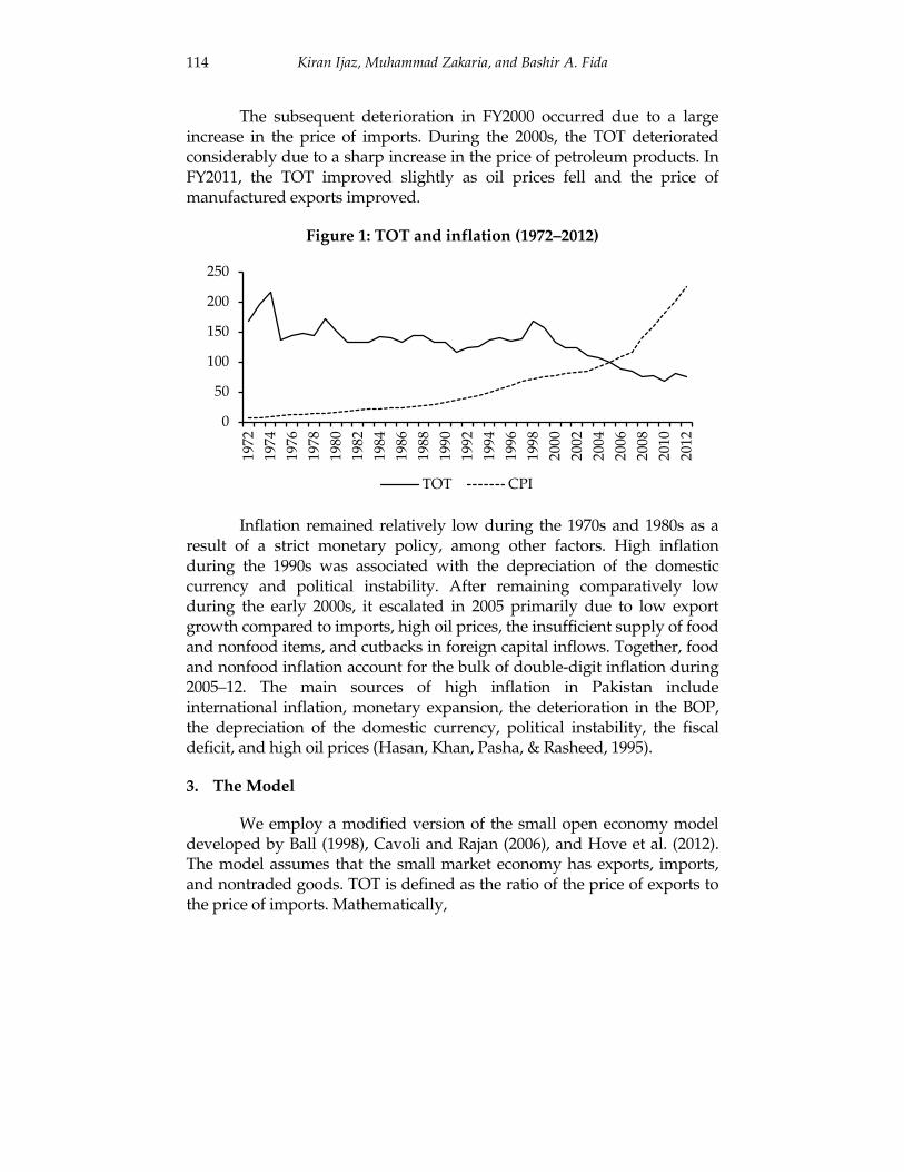
Figure 1 illustrates Pakistan’s TOT and inflation rate—measured by the consumer price index (CPI)—from 1972 to 2012. While the TOT has declined over time, the inflation rate has increased exponentially. In other words, we see a negative association between TOT and inflation, both of which have moved in opposite directions throughout this period. The TOT and inflation rate are negatively correlated both during Pakistan’s fixed exchange rate period (1972–81) and flexible exchange rate period (1982–2012). This is because the TOT has deteriorated under the flexible regime, causing both the nominal and real exchange rates to depreciate. As a result, inflation has increased.

The data for the 1970s exhibit more volatility in TOT than in inflation. The TOT improved in the fiscal year (FY) 1974 as a result of an increase in the value of exports. However, by FY1975, the situation had reversed and the TOT had deteriorated. The 1980s indicate a mixed trend, with the TOT improving as well as deteriorating. This pattern continued through the 1990s but improved in FY1998 when export values rose.


The subsequent deterioration in FY2000 occurred due to a large increase in the price of imports. During the 2000s, the TOT deteriorated considerably due to a sharp increase in the price of petroleum products. In FY2011, the TOT improved slightly as oil prices fell and the price of manufactured exports improved.

Figure 1: TOT and inflation (1972–2012)

Inflation remained relatively low during the 1970s and 1980s as a result of a strict monetary policy, among other factors. High inflation during the 1990s was associated with the depreciation of the domestic currency and political instability. After remaining comparatively low during the early 2000s, it escalated in 2005 primarily due to low export growth compared to imports, high oil prices, the insufficient supply of food and nonfood items, and cutbacks in foreign capital inflows. Together, food and nonfood inflation account for the bulk of double-digit inflation during 2005–12. The main sources of high inflation in Pakistan include international inflation, monetary expansion, the deterioration in the BOP, the depreciation of the domestic currency, political instability, the fiscal deficit, and high oil prices (Hasan, Khan, Pasha, & Rasheed, 1995).

3. The Model

We employ a modified version of the small open economy model developed by Ball (1998), Cavoli and Rajan (2006), and Hove et al. (2012). The model assumes that the small market economy has exports, imports, and nontraded goods. TOT is defined as the ratio of the price of exports to the price of imports. Mathematically,

0

50

100

150

200

250

1972

1974

1976

1978

1980

1982

1984

1986

1988

1990

1992

1994

1996

1998

2000

2002

2004

2006

2008

2010

2012

TOT CPI


Mt

Xt

t PP

TOT = (1)

The log of this equation is

which, can be written as

(2)

where

tott = log(TOTt ),

ptX = log(Pt

X ) , and

ptM = log(Pt

M ) .

Taking the first difference, we obtain

where

∆tott is the growth in TOT and

∆ptX (

∆ptM ) is the growth rate of the

domestic price of exports (imports). This equation can also be written as

(3)

where

π tX (= ∆pt

X ) is domestic exports inflation and

π tM (= ∆pt

M ) is domestic imports inflation.

We assume that the law of one price holds for both exports and imports. In the case of exports, this yields

where NER is the nominal exchange rate.

Taking the log, we obtain

which, is written as

)log()log()log( Mt

Xtt PPTOT −=

Mt

Xtt pptot −=

Mt

Xtt pptot ∆−∆=∆

Mt

Xtttot ππ −=∆

*Xt

Xt

t PP

NER =

)log()log()log( *Xt

Xtt PPNER −=

*Xt

Xtt ppner −=


where

nert = log(NERt ) ,

ptX = log(Pt

X ) , and

ptX * = log(Pt

X *) . Taking the first difference, we obtain

where

∆nert is the growth in the nominal exchange rate and

∆ptX (∆pt

X *) is the growth in the domestic (foreign) price of exports. Simple manipulation yields

which can also be written as

(4)

where )( Xt

Xt p∆=π is domestic exports inflation (the change in the domestic

price of exports) and )( ** Xt

Xt p∆=π is foreign exports inflation (the change

in the foreign price of exports), which we assume to be exogenous. Similarly, if the law of one price holds for imports, then

(5)

where Mtπ is domestic imports inflation (the change in the domestic price

of imports) and

π tM * is foreign imports inflation (the change in the foreign

price of imports). Substituting equations (4) and (5) into equation (3), we obtain

A simple computation yields

(6)

If the foreign price of imported goods is assumed to be related to the (general) foreign inflation rate, then the foreign price of imports will grow at the rate of foreign inflation, i.e.,

(7)

*Xt

Xtt ppner ∆−∆=∆

tXt

Xt nerpp ∆+∆=∆ *

tXt

Xt ner∆+= *ππ

tMt

Mt ner∆+= *ππ

)( **t

Mtt

Xtt nernertot ∆+−∆+=∆ ππ

** Mt

Xtttot ππ −=∆

**t

Mt ππ =


where

π tM * is foreign imports inflation and

π t* is the foreign inflation rate.

Substituting equation (7) into equation (6), we obtain

(8)

Rearranging the terms yields

(9)

The real exchange rate is the nominal exchange rate adjusted for domestic and foreign price levels. Mathematically,

where tRER is the real exchange rate and

Pt (Pt*) is the domestic (foreign)

inflation rate. Taking the log, we obtain

which, in lowercase letters, is written as

where )log( tt RERrer = , )log( tt NERner = , )log( **tt Pp = , and )log( tt Pp = .

Taking the first difference, we obtain

A notational change yields

(10)

where

∆rert is the growth in the real exchange rate,

∆nert is the growth in the nominal exchange rate,

π t*(= ∆pt

*) is the foreign inflation rate, and

π t (= ∆pt ) is the domestic inflation rate. Substituting equation (9) into equation (10) yields

(11)

**t

Xtttot ππ −=∆

tXtt tot∆−= ** ππ

t

ttt P

PNERRER

*

.=

)log()log()log()log( *tttt PPNERRER −+=

tttt ppnerrer −+= *

tttt ppnerrer ∆−∆+∆=∆ *

tttt nerrer ππ −+∆=∆ *

ttXttt totnerrer ∆−−+∆=∆ ππ *


After simple modification, this equation becomes

If we assume that 11 −− = tt nerrer θ , then rearranging the equation above will yield

(12)

This equation indicates that the real exchange rate is affected by the change in the nominal exchange rate, the change in price of foreign exported goods, domestic inflation, and the change in TOT.

The evolution of inflation takes the form of a Phillips curve as follows:

(13)

where 𝛾1,𝛾2, 𝛾3 and 𝛾4 are parameters while 𝜇𝑡 is the disturbance term. In this specification, the lagged inflation term captures inflation inertia, while the current and lagged output gap captures the contemporaneous as well as lagged transmission of output shocks to inflation. The real exchange rate affects inflation through import prices. Substituting equation (12) into equation (13), the above Phillips curve can be written as

ttttXttttt nernertotvyy υπβββπβββββπ ++++++++= −−− 17165

*431210 (14)

where tt tottotv ∆= is TOT volatility and the

βs are parameters to be estimated where

β1 = [γ1 /(1+ γ 3)] ,

β2 = [γ 2 /(1+ γ 3)] ,

β3 = [−γ 3 /(1+ γ 3)] ,

β4 = [γ 3 /(1+ γ 3)] ,

β5 = [γ 3 /(1+ γ 3)] ,

β6 = [γ 3(θ +1) /(1+ γ 3)] ,

β7 = [γ 4 /(1+ γ 3)], and

υt = [µt /(1+ γ 3)].

We also estimate the following augmented version of our model:

π t = β0 + β1 yt + β2 yt −1 + β3 totvt + β4 π tX * + β5 nert + β6 nert −1

+β7 π t −1 + β8 mst + β9 fdt + β10 oilt +υ t

(15)

where

mst is money supply,

fdt is the fiscal deficit, and

oilt represents oil prices. The theoretical justification for including these variables in the inflation equation is as follows:

ttXttttt totnernerrerrer ∆−−+−+= −− ππ *

11

ttXtttt totnernerrer ∆−−+−+= − ππθ *

1)1(

1 2 1 3 4 1t t t t t ty y rerπ γ γ γ γ π µ− −= + + + +


• Output growth (𝒚𝒕 ): Output growth can have both positive and negative effects on inflation. According to the quantity theory of money, as output increases, inflation decreases and vice versa. This implies that income affects inflation negatively. On the other hand, when income rises, the demand for money will also increase. As a result, the interest rate will rise, thereby increasing inflation (Fisher hypothesis). This indicates that income affects inflation positively. Some empirical studies show a negative relationship between income and inflation (see Ahmed & Murtaza, 2005; Ayyoub, Chaudhry, & Farooq, 2011); others show a positive relationship between income and inflation (see Malik & Chowdhury, 2001; Patra & Sahu, 2012).

• TOT volatility (𝒕𝒐𝒕𝒗𝒕): TOT volatility is expected to decrease inflation under a flexible exchange rate system by adjusting the real exchange rate. Further, high volatility in the TOT reduces investment by creating uncertainty. This will cause aggregate demand to fall, which will reduce inflation (Desormeaux et al., 2009). Some empirical studies find that TOT volatility has a negative effect on inflation (see Gruen & Shuetrim, 1994; Broda, 2004). Others have documented the positive effects of TOT volatility on inflation (see Andrews & Rees, 2009; Hove et al., 2012). This positive relationship between inflation and TOT volatility can be explained thus: when TOT volatility increases, exchange rate volatility will also rise. This will decrease foreign investment and trade, thereby reducing production and increasing inflation.

• Foreign export prices (𝝅𝒕𝑿∗): Theoretically, we expect foreign export

prices to have a positive effect on domestic inflation. Intuitively, foreign exports are domestic imports. As the price of foreign exports (domestic imports) increases, domestic inflation will rise and vice versa.

• Nominal exchange rate (𝒏𝒆𝒓𝒕): Under purchasing power parity, the exchange rate and inflation are positively correlated. A depreciation of the domestic currency will increase inflation while an appreciation will decrease inflation. Theoretically, the nominal exchange rate is expected to have a positive effect on inflation (see Ahmad & Ali, 1999; Ito & Sato, 2006).

• Money supply (𝒎𝒔𝒕): According to the quantity theory of money, when the money supply increases, inflation will also rise. Similarly, the monetarist view posits that inflation is a monetary phenomenon. Therefore, we expect the money supply to have a positive effect on inflation (in Pakistan’s context, see, for instance, Qayyum, 2006; Kemal, 2006).


• Fiscal deficit (𝒇𝒅𝒕 ): In Pakistan, the government either prints or borrows money to finance its fiscal deficit. These policies increase the money supply, ultimately causing inflation to rise in the country. Theoretically, the fiscal deficit should have a positive impact on inflation. Empirical studies on Pakistan also show this to be the case. A fiscal deficit indicates an excess of government spending over government revenues: this increases aggregate demand, thereby causing demand-pull inflation in the country (see Chaudhary & Ahmad, 1995; Agha & Khan, 2006; Fayyaz, Mughal, & Khan, 2011).

• Oil prices (𝒐𝒊𝒍𝒕): Pakistan depends heavily on imported oil to meet its energy needs. Therefore, an increase in the price of imported oil will increase the cost of production, in turn increasing domestic inflation. A number of studies reflect the positive effect of international oil prices on domestic inflation (see Kiani, 2008; O’Brien & Weymes, 2010; Khan & Ahmed, 2011).

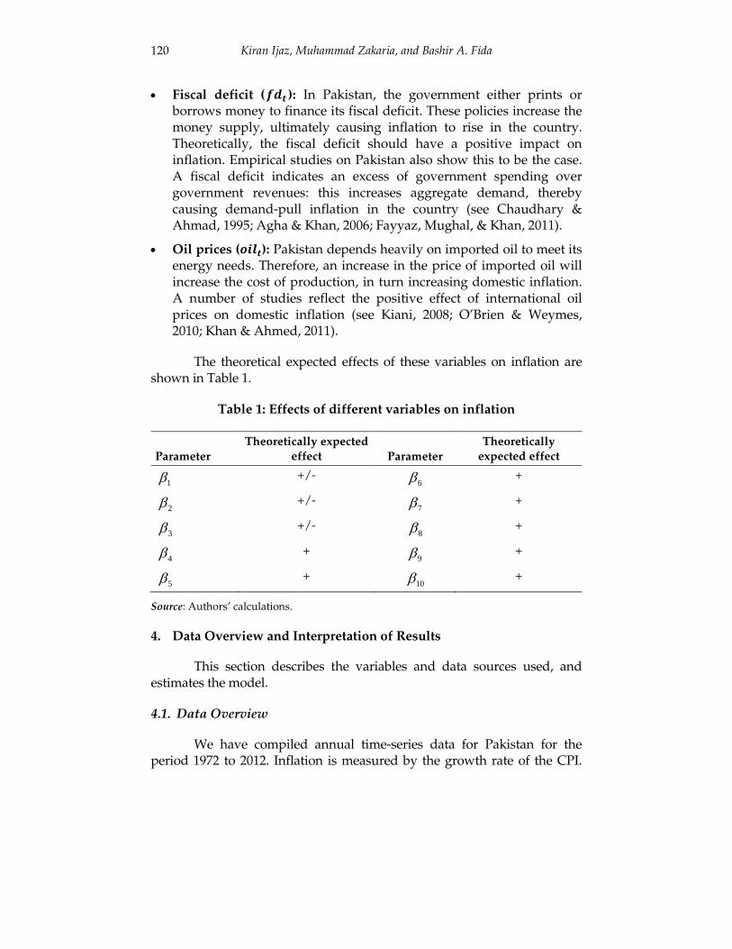
The theoretical expected effects of these variables on inflation are shown in Table 1.

Table 1: Effects of different variables on inflation

Parameter Theoretically expected

effect Parameter Theoretically

expected effect

+/-

+

+/-

+

+/-

+

+

+

+

+

Source: Authors’ calculations.

4. Data Overview and Interpretation of Results

This section describes the variables and data sources used, and estimates the model.

4.1. Data Overview

We have compiled annual time-series data for Pakistan for the period 1972 to 2012. Inflation is measured by the growth rate of the CPI.

1β 6β

2β 7β

3β 8β

4β 9β

5β 10β


Output growth is the real GDP growth rate. TOT volatility is measured using the autoregressive conditional heteroskedastic (ARCH) variance of TOT.1 Foreign exports inflation is calculated as the growth rate of the unit value index of exports of a foreign country (the US, in our study). The nominal exchange rate is expressed as the domestic currency per unit of foreign currency. Thus, an increase (decrease) in the the exchange rate implies a depreciation (appreciation) of the domestic currency. The money supply is the growth rate of broad money (M2). The fiscal deficit is taken as a percentage of GDP. The world oil price index acts as a proxy for international oil prices.

The data has been collected from the International Financial Statistics database, the State Bank of Pakistan’s (2010) Handbook of Statistics on Pakistan Economy, and the World Development Indicators database. Real variables and indices are calculated taking 2005 as the base year.

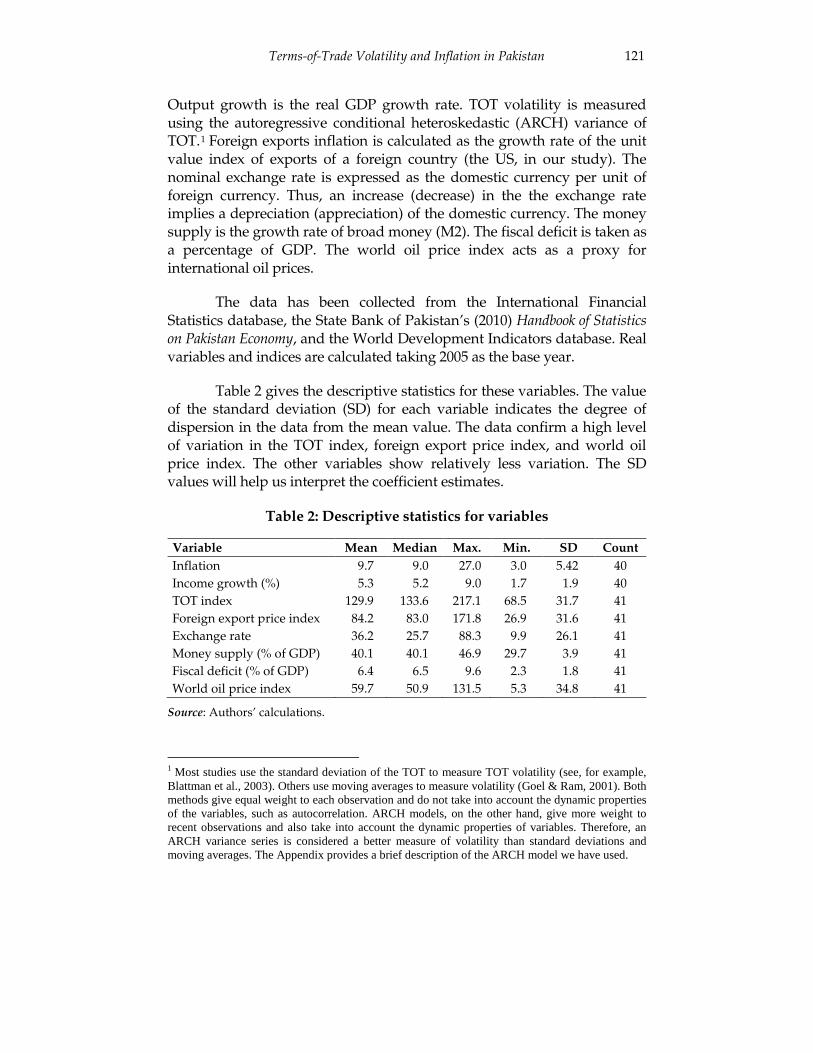
Table 2 gives the descriptive statistics for these variables. The value of the standard deviation (SD) for each variable indicates the degree of dispersion in the data from the mean value. The data confirm a high level of variation in the TOT index, foreign export price index, and world oil price index. The other variables show relatively less variation. The SD values will help us interpret the coefficient estimates.

Table 2: Descriptive statistics for variables

Variable Mean Median Max. Min. SD Count Inflation 9.7 9.0 27.0 3.0 5.42 40 Income growth (%) 5.3 5.2 9.0 1.7 1.9 40 TOT index 129.9 133.6 217.1 68.5 31.7 41 Foreign export price index 84.2 83.0 171.8 26.9 31.6 41 Exchange rate 36.2 25.7 88.3 9.9 26.1 41 Money supply (% of GDP) 40.1 40.1 46.9 29.7 3.9 41 Fiscal deficit (% of GDP) 6.4 6.5 9.6 2.3 1.8 41 World oil price index 59.7 50.9 131.5 5.3 34.8 41


1 Most studies use the standard deviation of the TOT to measure TOT volatility (see, for example, Blattman et al., 2003). Others use moving averages to measure volatility (Goel & Ram, 2001). Both methods give equal weight to each observation and do not take into account the dynamic properties of the variables, such as autocorrelation. ARCH models, on the other hand, give more weight to recent observations and also take into account the dynamic properties of variables. Therefore, an ARCH variance series is considered a better measure of volatility than standard deviations and moving averages. The Appendix provides a brief description of the ARCH model we have used.


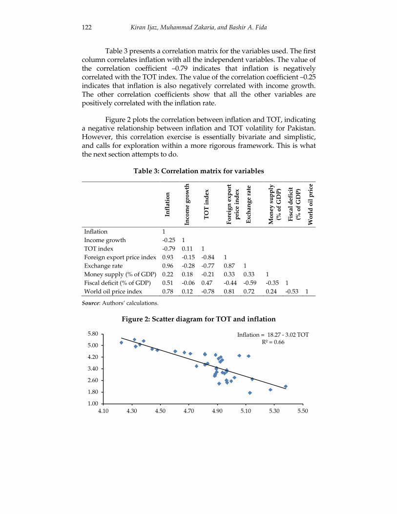
Table 3 presents a correlation matrix for the variables used. The first column correlates inflation with all the independent variables. The value of the correlation coefficient –0.79 indicates that inflation is negatively correlated with the TOT index. The value of the correlation coefficient –0.25 indicates that inflation is also negatively correlated with income growth. The other correlation coefficients show that all the other variables are positively correlated with the inflation rate.

Figure 2 plots the correlation between inflation and TOT, indicating a negative relationship between inflation and TOT volatility for Pakistan. However, this correlation exercise is essentially bivariate and simplistic, and calls for exploration within a more rigorous framework. This is what the next section attempts to do.

Table 3: Correlation matrix for variables

Infl

atio

n

Inco

me

grow

th

TO

T in

dex

Fore

ign

exp

ort

pric

e in

dex

Exch

ange

rat

e

Mon

ey s

uppl

y (%

of

GD

P)

Fisc

al d

efic

it

(% o

f GD

P)

Wor

ld o

il p

rice

Inflation 1 Income growth -0.25 1 TOT index -0.79 0.11 1 Foreign export price index 0.93 -0.15 -0.84 1 Exchange rate 0.96 -0.28 -0.77 0.87 1 Money supply (% of GDP) 0.22 0.18 -0.21 0.33 0.33 1 Fiscal deficit (% of GDP) 0.51 -0.06 0.47 -0.44 -0.59 -0.35 1 World oil price index 0.78 0.12 -0.78 0.81 0.72 0.24 -0.53 1


Figure 2: Scatter diagram for TOT and inflation

Inflation = 18.27 - 3.02 TOT R² = 0.66

1.00

1.80

2.60

3.40

4.20

5.00

5.80

4.10 4.30 4.50 4.70 4.90 5.10 5.30 5.50


4.2. Estimation and Interpretation of Model

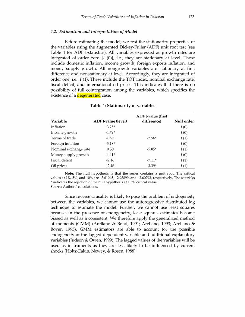
Before estimating the model, we test the stationarity properties of the variables using the augmented Dickey-Fuller (ADF) unit root test (see Table 4 for ADF t-statistics). All variables expressed as growth rates are integrated of order zero [I (0)], i.e., they are stationary at level. These include domestic inflation, income growth, foreign exports inflation, and money supply growth. All nongrowth variables are stationary at first difference and nonstationary at level. Accordingly, they are integrated of order one, i.e., I (1). These include the TOT index, nominal exchange rate, fiscal deficit, and international oil prices. This indicates that there is no possibility of full cointegration among the variables, which specifies the existence of a degenerated case.

Table 4: Stationarity of variables

Variable ADF t-value (level) ADF t-value (first

difference) Null order Inflation -3.25* I (0) Income growth -4.79* I (0) Terms of trade -0.93 -7.56* I (1) Foreign inflation -5.18* I (0) Nominal exchange rate 0.50 -5.85* I (1) Money supply growth -4.41* I (0) Fiscal deficit -2.16 -7.11* I (1) Oil prices -2.46 -3.39* I (1)

Note: The null hypothesis is that the series contains a unit root. The critical values at 1%, 5%, and 10% are –3.61045, –2.93899, and –2.60793, respectively. The asterisks * indicates the rejection of the null hypothesis at a 5% critical value. Source: Authors’ calculations.

Since reverse causality is likely to pose the problem of endogeneity between the variables, we cannot use the autoregressive distributed lag technique to estimate the model. Further, we cannot use least squares because, in the presence of endogeneity, least squares estimates become biased as well as inconsistent. We therefore apply the generalized method of moments (GMM) (Arellano & Bond, 1991; Arellano, 1993; Arellano & Bover, 1995). GMM estimators are able to account for the possible endogeneity of the lagged dependent variable and additional explanatory variables (Judson & Owen, 1999). The lagged values of the variables will be used as instruments as they are less likely to be influenced by current shocks (Holtz-Eakin, Newey, & Rosen, 1988).


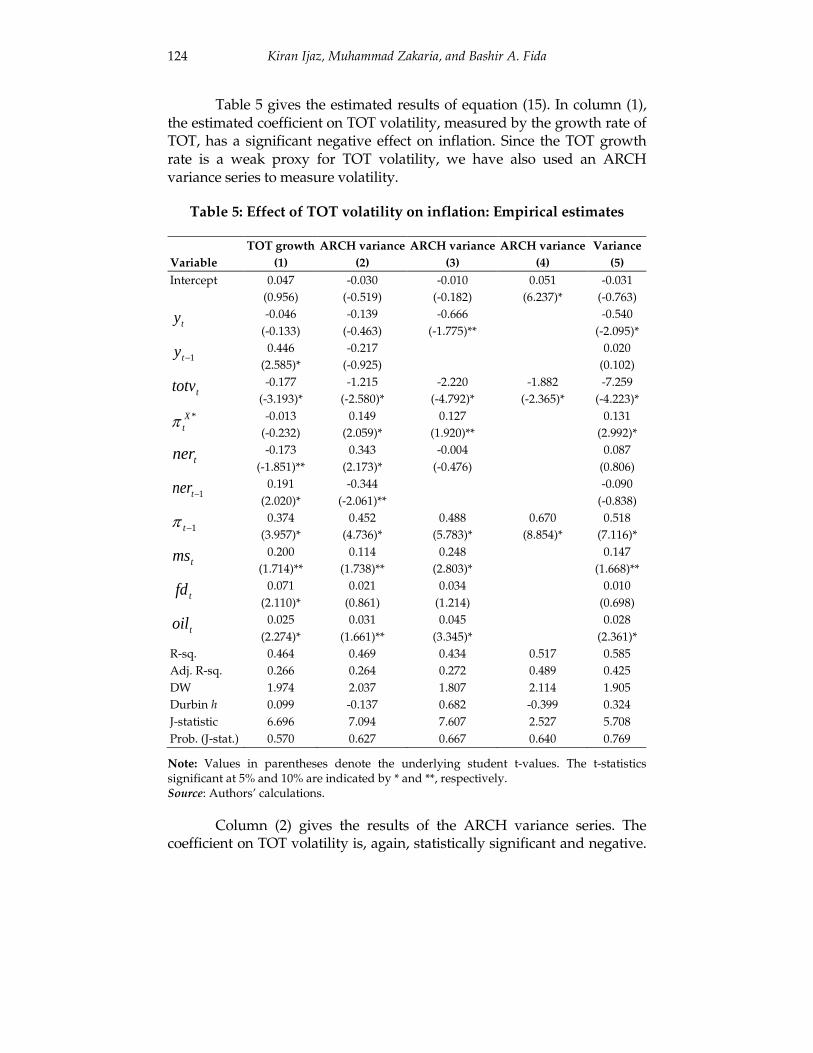
Table 5 gives the estimated results of equation (15). In column (1), the estimated coefficient on TOT volatility, measured by the growth rate of TOT, has a significant negative effect on inflation. Since the TOT growth rate is a weak proxy for TOT volatility, we have also used an ARCH variance series to measure volatility.

Table 5: Effect of TOT volatility on inflation: Empirical estimates

Variable TOT growth ARCH variance ARCH variance ARCH variance Variance

(1) (2) (3) (4) (5) Intercept 0.047 -0.030 -0.010 0.051 -0.031

(0.956) (-0.519) (-0.182) (6.237)* (-0.763)

ty -0.046 -0.139 -0.666 -0.540 (-0.133) (-0.463) (-1.775)** (-2.095)*

1−ty 0.446 -0.217 0.020 (2.585)* (-0.925) (0.102)

ttotv -0.177 -1.215 -2.220 -1.882 -7.259 (-3.193)* (-2.580)* (-4.792)* (-2.365)* (-4.223)*

*Xtπ -0.013 0.149 0.127 0.131

(-0.232) (2.059)* (1.920)** (2.992)*

tner -0.173 0.343 -0.004 0.087 (-1.851)** (2.173)* (-0.476) (0.806)

1−tner 0.191 -0.344 -0.090 (2.020)* (-2.061)** (-0.838)

1−tπ 0.374 0.452 0.488 0.670 0.518 (3.957)* (4.736)* (5.783)* (8.854)* (7.116)*

tms 0.200 0.114 0.248 0.147 (1.714)** (1.738)** (2.803)* (1.668)**

tfd 0.071 0.021 0.034 0.010 (2.110)* (0.861) (1.214) (0.698)

toil 0.025 0.031 0.045 0.028 (2.274)* (1.661)** (3.345)* (2.361)*

R-sq. 0.464 0.469 0.434 0.517 0.585 Adj. R-sq. 0.266 0.264 0.272 0.489 0.425 DW 1.974 2.037 1.807 2.114 1.905 Durbin h 0.099 -0.137 0.682 -0.399 0.324 J-statistic 6.696 7.094 7.607 2.527 5.708 Prob. (J-stat.) 0.570 0.627 0.667 0.640 0.769

Note: Values in parentheses denote the underlying student t-values. The t-statistics significant at 5% and 10% are indicated by * and **, respectively. Source: Authors’ calculations.

Column (2) gives the results of the ARCH variance series. The coefficient on TOT volatility is, again, statistically significant and negative.


The estimated value of the coefficient indicates that a one-percent increase in TOT volatility will decrease inflation by 1.215 percent. This implies that TOT volatility had a deflationary effect in Pakistan during the study period. One possible reason for this is that the volatile TOT adversely affected external trade and foreign investment, creating the deflationary impact. Further, Pakistan exports mainly agricultural products and imports capital goods: the price of the former fluctuates more than that of the latter, creating high volatility in TOT and discouraging agricultural good exports. This has a deflationary effect by decreasing aggregate demand.

Column (3) gives the results we obtain when the lagged terms of output growth and nominal exchange rate are excluded from the model to remove the possibility of multicollinearity. In this case, the coefficient on TOT volatility remains negative and statistically significant. Column (4) gives the results estimated exclusively for TOT volatility. The effect of TOT volatility on inflation is negative and statistically significant as the estimated value of the coefficient indicates (–1.882). Column (5) gives the results we obtain when TOT volatility is calculated by the simple variance of TOT. Here, again, the effect of TOT volatility on inflation is not only negative but also statistically significant. This indicates that the effect of TOT volatility on inflation is robust to alternative equation specifications and different measures of TOT volatility.

As far as the impact of the other control variables on inflation is concerned, output growth has a negative but statistically insignificant effect as shown in column (2).2 Conversely, this result is significant both in columns (3) and (5). This result supports the quantity theory of money hypothesis, which posits that, as income increases, inflation decreases. The effect of previous-period output growth on inflation is statistically insignificant both in columns (2) and (5).

As expected in theory, the effect of foreign export prices on domestic inflation is positive and statistically significant. The estimated value of the coefficient indicates that a one-percent rise in foreign export prices will increase domestic inflation by 0.149 percent as shown in column (2). Alternatively, a one-SD rise in foreign exports inflation (31.6) will increase domestic inflation by 4.708 points. This result is robust to alternative equation specifications as shown in the other columns.

A depreciation of the domestic currency increases inflation as the significant positive value of the coefficient on the nominal exchange rate

2 All interpretations refer to columns (2) to (5) only.


indicates in column (2). Thus, if the Pakistan rupee depreciates by 1 percent, domestic inflation will increase by 0.343 percent. However, this result is statistically insignificant in columns (3) and (5). Conversely, the lagged value of the nominal exchange rate has a significant negative effect on inflation. Again, this result is not, however, robust to alternative equation specifications.

Inflation is statistically positively correlated with its lagged value. Further, as theoretically expected, inflation increases with a rise in money supply. The estimated value of the coefficient indicates that a one-percent rise in money supply will increase inflation by 0.114 percent. Alternatively, a one-SD increase in money supply (3.9) will increase inflation by 0.445 units. This result is not only significant but also robust to alternative equation specifications, and implies that the quantity theory of money hypothesis holds for Pakistan, i.e., inflation increases with an increase in money supply.

As discussed earlier, there may be differential effects under fixed and flexible exchange rates. Pakistan followed a fixed rate regime till 1981 and then moved to a flexible system. The dummy incorporated to account for this was statistically insignificant and thus removed from the model. Further, we have only 10 observations for the fixed exchange rate (1972–1981) and 31 observations for the flexible regime (1982–2012).

The fiscal deficit has a positive effect on inflation: a one-percent increase in the fiscal deficit will increase inflation by 0.021 percent. However, this result is statistically insignificant and remains so in the other specifications as well. Finally, the international oil price has a significant positive effect on inflation: if oil prices increase by 1 percent in the international market, domestic inflation will rise by 0.031 percent. This result is robust to alternative equation specifications.

The high values of 2R and the adjusted 2R indicate that the model

fits the data well. The Durbin Watson statistic values are close to the desired value of 2, which indicates the absence of autocorrelation. Since the lagged value of the dependent variable is included as an independent variable, we have also calculated Durbin h statistics, the values of which are less than 1.96 in absolute terms. Again, this indicates a lack of autocorrelation in the model. We check the validity of the instruments using the J-test: the high p-values of the J-statistics indicate that the instruments are valid. Further, the high value of the F-statistic indicates that the model fits the data well.


5. Conclusion

This study has empirically examined the effect of TOT volatility on inflation in Pakistan using annual data for the period 1972 to 2012. To control for potential endogeneity, we have employed the GMM technique. The estimated results show that TOT volatility has a significant negative effect on inflation in Pakistan. The estimated value of the coefficient on TOT volatility indicates that a one-percent increase in TOT volatility will reduce inflation by 1.215 percent. This result is robust to alternative equation specifications and TOT volatility measures.

The control variables used have the theoretical impact we expect. Output growth has a significant negative effect while the foreign exports price has a significant positive effect on domestic inflation. A depreciation of the nominal exchange rate or money supply increases the inflation rate. The positive significant influence of the money supply on domestic inflation corresponds somewhat to the monetarist view that money is the most important variable affecting the inflationary process. The fiscal deficit and world oil prices are also found to increase inflation in the country.

This study has some important policy implications. Inflation in Pakistan can be cured by maintaining a stable TOT. Foreign export prices (or domestic import prices) increase inflation, which implies that decreasing Pakistan’s dependency on foreign imports would help reduce inflation. Further, appreciating the nominal exchange rate, tightening monetary policy, curtailing the fiscal deficit, and reducing oil prices would help curb inflation. Although the government has taken some recent steps to appreciate the domestic currency, much more needs to be done.


References

Abdullah, M., & Kalim, R. (2012). Empirical analysis of food price inflation in Pakistan. World Applied Sciences Journal, 16(7), 933–939.

Agha, A. I., & Khan, M. S. (2006). An empirical analysis of fiscal imbalances and inflation in Pakistan. SBP Research Bulletin, 2(2), 343–362.

Ahmad, E., & Ali, S. A. (1999). Exchange rate and inflation dynamics. Pakistan Development Review, 38(3), 235–251.

Ahmed, S., & Murtaza, M. G. (2005). Inflation and economic growth in Bangladesh: 1981–2005 (Working Paper No. 0604). Dhaka: Bangladesh Bank, Policy Analysis Unit.

Andrews, D., & Rees, D. (2009). Macroeconomic volatility and terms of trade shocks (Research Discussion Paper No. 2009-05). Sydney: Reserve Bank of Australia.

Arellano, M. (1993). On the testing of correlated effects with panel data. Journal of Econometrics, 59(1–2), 87–97.

Arellano, M., & Bond, S. (1991). Some tests of specification for panel data: Monte Carlo evidence and an application to employment equations. Review of Economic Studies, 58(2), 277–297.

Arellano, M., & Bover, O. (1995). Another look at the instrumental variable estimation of error-components models. Journal of Econometrics, 68(1), 29–51.

Ayyoub, A., Chaudhry, I. S., & Farooq, F. (2011). Does inflation affect economic growth? Pakistan Journal of Social Sciences, 31(1), 51–64.

Ball, L. M. (1998). Policy rules for open economies (Working Paper No. 6760). Cambridge, MA: NBER.

Baxter, M., & Kouparitsas, M. A. (2000). What causes fluctuations in the terms of trade? (Working Paper No. 7462). Cambridge, MA: National Bureau of Economic Research.


Blattman, C., Hwang, J., & Williamson, J. G. (2003). The terms of trade and economic growth in the periphery 1870–1983 (Working Paper No. 9940). Cambridge, MA: National Bureau of Economic Research.

Bleaney, M., & Greenway, D. (2001). The impact of terms of trade and real exchange volatility on investment and growth in sub-Saharan Africa. Journal of Development Economics, 65(2), 491–500.

Broda, C. (2004). Terms of trade and exchange rate regimes in developing countries. Journal of International Economics, 63(1), 31–58.

Broda, C., & Tille, C. (2003). Coping with terms-of-trade shocks in developing countries. Current Issues in Economics and Finance, 9(11), 1–7.

Cavoli, T., & Rajan, R. S. (2006). Monetary policy rules for small and open developing economies: A counterfactual policy analysis. Journal of Economic Development, 31(1), 89–11.

Chaudhary, M. A., & Ahmad, N. (1995). Money supply, deficit, and inflation in Pakistan. Pakistan Development Review, 34(4), 945–956.

Desormeaux, J., García, P., & Soto, C. (2010). Terms of trade, commodity prices and inflation dynamics in Chile. In Bank for International Settlements (Ed.), Monetary policy and the measurement of inflation: Prices, wages and expectations (vol. 49). Basel, Switzerland: Bank for International Settlements.

Durevall, D., & Ndung’u, N. S. (1999). A dynamic model of inflation for Kenya: 1974–1996 (Working Paper No. 99/97). Washington, DC: International Monetary Fund.

Fatima, N. (2010). Analyzing the terms of trade effect for Pakistan (Working Paper No. 2010-59). Islamabad: Pakistan Institute of Development Economics.

Fayyaz, A., Mughal, K., & Khan, M. A. (2011). Fiscal deficit and its impact on inflation, causality and cointegration: The experience of Pakistan (1960–2010). Far East Journal of Psychology and Business, 5(3), 51–62.


Goel, R. K., & Ram, R. (2001). Irreversibility of R&D investment and the adverse effect of uncertainty: Evidence from the OECD countries. Economics Letters, 71, 287–291.

Gruen, D., & Dwyer, J. (1995). Are terms of trade rises inflationary? (Research Discussion Paper No. 9508). Sydney: Reserve Bank of Australia.

Gruen, D., & Shuetrim, G. (1994). Internationalization and the macro-economy. In P. Lowe & J. Dwyer (Eds.), International integration of the Australian economy: Proceedings of a conference (pp. 309–363). Sydney: Reserve Bank of Australia.

Hasan, M. A., Khan, A. H., Pasha, H. A., & Rasheed, M. A. (1995). What explains the current high rate of inflation in Pakistan? Pakistan Development Review, 34(4), 927–943.

Holtz-Eakin, D., Newey, W., & Rosen, H. S. (1988). Estimating vector autoregressions with panel data. Econometrica, 56(6), 1371–1395.

Hove, S., Mama, A. T., & Tchana, F. T. (2012). Terms of trade shocks and inflation targeting in emerging market economies (Working Paper No. 273). Cape Town: Economic Research Southern Africa.

Ito, T., & Sato, K. (2006). Exchange rate changes and inflation in post-crisis Asian economies: VAR analysis of the exchange rate pass-through (Working Paper No. 12395). Cambridge, MA: National Bureau of Economic Research.

Jääskelä, J., & Smith, P. (2011). Terms of trade shocks: What are they and what do they do? (Research Discussion Paper No. 2011-5). Sydney: Reserve Bank of Australia.

Judson, R. A., & Owen, A. L. (1999). Estimating dynamic panel data models: A guide for macroeconomists. Economics Letters, 65(1), 9–15.

Kemal, M. A. (2006). Is inflation in Pakistan a monetary phenomenon? Pakistan Development Review, 45(2), 213–220.

Khan, A. R., & Ahmed, A. (2011). Macroeconomic effects of global food and oil price shocks to the Pakistan economy: A structural vector autoregressive analysis. Pakistan Development Review, 50(4), 491–511.


Khan, A., Bukhari, S., & Ahmed, Q. (2007). Determinants of recent inflation in Pakistan (Research Report No. 66). Karachi, Pakistan: Social Policy and Development Center.

Kiani, A. (2008). Impact of high oil prices on Pakistan’s economic growth. International Journal of Business and Social Science, 2(17), 209–216.

Malik, G., & Chowdhury, A. (2001). Inflation and economic growth: Evidence from four South Asian countries. Asia-Pacific Development Journal, 8(1), 123–135.

Mendoza, E. G. (1995). The terms of trade, the real exchange rate, and economic fluctuations. International Economic Review, 36(1), 101–137.

O’Brien, D., & Weymes, L. (2010, July). The impact of oil prices on Irish inflation. Quarterly Bulletin (Central Bank of Ireland), 3, 66–82.

Patra, S., & Sahu, K. K. (2012). Inflation in South Asia and its macroeconomic linkages. Journal of Arts, Science and Commerce, 3(2), 10–15.

Qayyum, A. (2006). Money, inflation, and growth in Pakistan. Pakistan Development Review, 45(2), 203–212.


Appendix

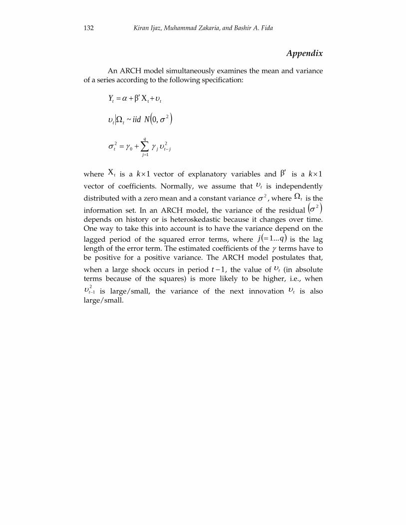
An ARCH model simultaneously examines the mean and variance of a series according to the following specification:

ttY υα +′+= tXβ

( )20, ~ συ Niidtt Ω

∑=

−+=q

jjtjt

1

20

2 υγγσ

where tX is a 1×k vector of explanatory variables and β′ is a 1×k

vector of coefficients. Normally, we assume that tυ is independently

distributed with a zero mean and a constant variance 2σ , where tΩ is the

information set. In an ARCH model, the variance of the residual ( )2σ depends on history or is heteroskedastic because it changes over time. One way to take this into account is to have the variance depend on the lagged period of the squared error terms, where ( )qj ...1= is the lag length of the error term. The estimated coefficients of the

γ terms have to be positive for a positive variance. The ARCH model postulates that,

when a large shock occurs in period 1−t , the value of tυ (in absolute terms because of the squares) is more likely to be higher, i.e., when

21−tυ is large/small, the variance of the next innovation tυ is also

large/small.

terms-of-trade volatility and inflation in pakistan … · terms-of-trade volatility and inflation...

Documents