terrain avoidance nonlinear model predictive control for autonomous rotorcraft

7/28/2019 Terrain Avoidance Nonlinear Model Predictive Control for Autonomous Rotorcraft

http://slidepdf.com/reader/full/terrain-avoidance-nonlinear-model-predictive-control-for-autonomous-rotorcraft 1/17

J Intell Robot Syst (2012) 68:69–85

DOI 10.1007/s10846-012-9669-6

Terrain Avoidance Nonlinear Model Predictive Control

for Autonomous RotorcraftBruno J. N. Guerreiro · Carlos Silvestre · Rita Cunha

Received: 15 September 2010 / Accepted: 4 March 2012 / Published online: 25 March 2012© Springer Science+Business Media B.V. 2012

Abstract This paper describes a terrain avoidance

control methodology for autonomous rotorcraft

applied to low altitude flight. A simple nonlinear

model predictive control (NMPC) formulation is

used to adequately address the terrain avoidance

problem, which involves stabilizing a nonlinear

and highly coupled dynamic model of a helicopter,

while avoiding collisions with the terrain as well

as preventing input and state saturations. The

This work was partially supported by project FCT[PEst-OE/EEI/LA0009/2011], by project FCTAMMAIA (PTDC/HIS-ARQ/103227/2008), and byproject AIRTICI from AdI through the POSConhecimento Program that includes FEDER funds.The work of Bruno Guerreiro was supported by thePhD Student Grant SFRH/BD/21781/2005 from thePortuguese FCT POCTI program.

B. J. N. Guerreiro (B) · C. Silvestre · R. CunhaInstitute for Systems and Robotics (ISR),

Instituto Superior Técnico (IST),Torre Norte Piso 8, Av. Rovisco Pais 1,1049-001 Lisbon, Portugale-mail: [email protected]

C. Silvestree-mail: [email protected]

R. Cunhae-mail: [email protected]

C. SilvestreFaculty of Science and Technology,University of Macau, Taipa, Macau

physical input saturations are made intrinsic to the

model, such that the control is always admissible

and the MPC design is simplified. A comparison

of several optimization approaches is provided,

where the performance of the traditional gradi-

ent method with fixed step is compared with the

quasi-Newton method and a line search algorithm.

The simulation results show that the adopted

strategy achieves good performance even when

the desired path is on collision course with the

terrain.

Keywords Helicopter control ·

Obstacle avoidance · Model-based control ·

Predictive control · Nonlinear models

Mathematics Subject Classification (2010) 49J15 ·

49N90

1 Introduction

This paper addresses the problem of low altitude

terrain avoidance flight control of autonomous

rotorcraft. Within the scope of Unmanned Aer-

ial Vehicles, autonomous rotorcraft have been

steadily growing as a major topic of research. They

have the potential to perform high precision tasks

in challenging and uncertain operation scenar-

ios as new sensor technology and increasingly

powerful computational systems are available.



70 J Intell Robot Syst (2012) 68:69–85

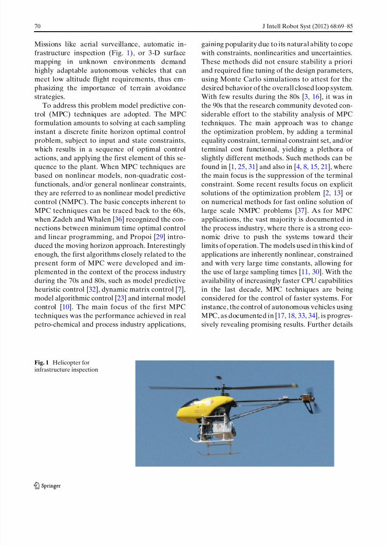
Missions like aerial surveillance, automatic in-

frastructure inspection (Fig. 1), or 3-D surface

mapping in unknown environments demand

highly adaptable autonomous vehicles that can

meet low altitude flight requirements, thus em-

phasizing the importance of terrain avoidance

strategies.To address this problem model predictive con-

trol (MPC) techniques are adopted. The MPC

formulation amounts to solving at each sampling

instant a discrete finite horizon optimal control

problem, subject to input and state constraints,

which results in a sequence of optimal control

actions, and applying the first element of this se-

quence to the plant. When MPC techniques are

based on nonlinear models, non-quadratic cost-

functionals, and/or general nonlinear constraints,

they are referred to as nonlinear model predictivecontrol (NMPC). The basic concepts inherent to

MPC techniques can be traced back to the 60s,

when Zadeh and Whalen [36] recognized the con-

nections between minimum time optimal control

and linear programming, and Propoi [29] intro-

duced the moving horizon approach. Interestingly

enough, the first algorithms closely related to the

present form of MPC were developed and im-

plemented in the context of the process industry

during the 70s and 80s, such as model predictive

heuristic control [32], dynamic matrix control [7],model algorithmic control [23] and internal model

control [10]. The main focus of the first MPC

techniques was the performance achieved in real

petro-chemical and process industry applications,

gaining popularity due to its natural ability to cope

with constraints, nonlinearities and uncertainties.

These methods did not ensure stability a priori

and required fine tuning of the design parameters,

using Monte Carlo simulations to attest for the

desired behavior of the overall closed loop system.

With few results during the 80s [3, 16], it was inthe 90s that the research community devoted con-

siderable effort to the stability analysis of MPC

techniques. The main approach was to change

the optimization problem, by adding a terminal

equality constraint, terminal constraint set, and/or

terminal cost functional, yielding a plethora of

slightly different methods. Such methods can be

found in [1, 25, 31] and also in [4, 8, 15, 21], where

the main focus is the suppression of the terminal

constraint. Some recent results focus on explicit

solutions of the optimization problem [2, 13] oron numerical methods for fast online solution of

large scale NMPC problems [37]. As for MPC

applications, the vast majority is documented in

the process industry, where there is a strong eco-

nomic drive to push the systems toward their

limits of operation. The models used in this kind of

applications are inherently nonlinear, constrained

and with very large time constants, allowing for

the use of large sampling times [11, 30]. With the

availability of increasingly faster CPU capabilities

in the last decade, MPC techniques are beingconsidered for the control of faster systems. For

instance, the control of autonomous vehicles using

MPC, as documented in [17, 18, 33, 34], is progres-

sively revealing promising results. Further details

Fig. 1 Helicopter forinfrastructure inspection



J Intell Robot Syst (2012) 68:69–85 71

on the theoretical developments and applications

of MPC techniques can be found in [9, 11, 20, 22].

Related work using different control methodo-

logies in the context of terrain following for

autonomous helicopters, can be found in [28]. The

authors use gain-scheduling control techniques to

control and guide the vehicle, in such a way thatit is possible to incorporate preview information

to achieve terrain following. In [19], an MPC-

based nap-of-earth flight trajectory optimization

for a helicopter is designed, resorting to an input-

output mapping of control functions and resultant

system trajectories, while in [35], MPC obstacle

avoidance techniques are applied in the field of

autonomous ground vehicles.

In this paper a simple NMPC methodology

is proposed in order to simultaneously meet the

conflicting control objectives of trajectory track-ing and terrain avoidance. Since in NMPC the

optimal control problem is solved on-line, it is

straightforward to add state saturation constraints

as a penalty function to the cost functional and the

vehicle dynamic model constraint can be readily

incorporated in the cost functional using Lagrange

multipliers. In an effort to simplify the optimiza-

tion algorithm, the input saturation is directly

incorporated in the nonlinear model instead of

being added as a constraint to the optimization

problem. To enforce the terrain avoidance, a vir-tual repulsive field is defined around the heli-

copter such that any obstacle within its range is

weighted in the optimal control cost functional,

guiding the vehicle trajectory away from colli-

sions. The resulting unconstrained optimization

problem is then numerically solved using the

gradient and quasi-Newton methods to compute

the search direction and using the Wolfe condi-

tions for the line search algorithm to solve the

step size optimization subproblem [26]. The ve-

hicle model considered in this work is a heli-

copter nonlinear dynamic model, derived from

first-principles and specially suited for model-

scale helicopters [5, 6]. The control algorithm re-

lies on a simplified version of the referred model

to compute the sequence of state vectors given a

sequence of input vectors.

The key contribution of this work is the use

of simple and well established optimization tech-

niques to solve the terrain avoidance trajectory

tracking NMPC problem for a complex nonlinear

helicopter model. The comparison of the gradient

method with fixed step size and the quasi-Newton

method with line search provides evidence that

the later optimization approach is a simple yet

effective way to reduce the computation burden

inherent to NMPC techniques. Furthermore, theintrinsic saturation described in this paper sim-

plifies the controller design by removing the need

to include input constraints in the optimization

problem.

The paper is organized as follows. Section 2

presents a brief summary of the helicopter dy-

namic model, including the intrinsic actuation

saturation functions, the discretization and the

time delay modeling. Section 3 formulates the

terrain avoidance NMPC problem, describing

the control problem, the optimization algorithmand the saturation, terrain and model constraints.

Implementation issues and simulation results are

presented in Section 4. Section 5 summarizes the

main ideas of this paper and discusses directions

for future work. A preliminary version of these

results was presented at the 17th IFAC World

Congress and can be found in [14].

2 Helicopter Model

This section briefly describes the helicopter dy-

namic model, as well as the intrinsic input satu-

ration, the discretization and the time delay

modeling. A comprehensive coverage of heli-

copter flight dynamics can be found in [5, 27]

and [6].

Consider the helicopter modeled as a rigid body

driven by the resultant force and moment ap-

plied at the helicopter’s center of mass, which

include the contributions of the helicopter com-ponents and gravitational force. Let

I pB, I BR

∈

SE(3) R3 × SO(3) denote the configuration of

the body frame {B} (attached to the vehicle’s

center of mass) with respect to the inertial

frame { I }. Consider also the Euler angles vec-

tor λB =

φB θ B ψB

, denoting the orientation

of {B} relative to { I } such that I BR = R(λB),

where θ B ∈ (− π2

, π2

] and φB, ψB ∈ R. The linear

and angular body velocities are defined as vB and




ωB, respectively, where vB = B I R

I pB ∈ R3, ωB =B I R

I ωB and I ωB is the angular velocity of {B}

relative to { I }. For the sake of simplicity, the

superscript of the position vector is dropped, so

that pB = I pB, and the time dependence of the

state and input variables is omitted.

Using this notation, the helicopter combineddynamics and kinematics state equations can be

written as

⎧⎪⎪⎪⎪⎪⎪⎪⎪⎨⎪⎪⎪⎪⎪⎪⎪⎪⎩

vB = −ωB × vB

+1

m

f h (vB,ωB, uB) + f g (φB, θ B)

ωB = −I−1 (ωB × IωB)+I−1 nh (vB,ωB, uB)

pB = R (λB) vB

λB = Q (λB) ωB

.

(1)

In the above equations, m denotes the vehicle

mass, I is the tensor of inertia about the frame {B},

uB is the input vector, f h and nh are the external

force and moment vectors due to the helicopter

components, and f g stands for the gravitational

force vector, all expressed in body coordinates,

and Q is the transformation from angular rates to

Euler angle derivatives. The state vector is defined

as xB = [vB ω

B pB λ

B], noting that xB ∈ X ⊂ Rn x

with n x = 12. The input vector, uB ∈ U ⊂ Rnu withnu = 4, is defined as uB =

θ c0

θ c1cθ c1 s

θ c0t

and

comprises the main rotor collective input θ c0, the

main rotor cyclic inputs θ c1cand θ c1 s

, and the tail

rotor collective input θ c0t .

There are five main components on a helicopter

that contribute for the overall force and moment

vectors: main rotor, tail rotor, fuselage, horizontal

tail plane and vertical tail fin, respectively denoted

by the subscripts mr , tr , f us, tp and f n. Hence,

the force and moment vectors can be decomposed

as f h = f mr + f tr + f f us + f tp + f fn and nh = nmr +ntr + n fus + ntp + n f n.

2.1 Main Rotor

As the primary source of lift, propulsion and

control, the main rotor dominates the helicopter

dynamic behavior. As a result of the aerodynamic

lift forces generated at the surface of its blades,

the main rotor is responsible for the helicopter’s

distinctive ability to operate in low-speed regimes,

which include hovering and vertical maneuvering.

To present the main rotor equations of motion,

two additional frames need to be introduced. The

first denotes the Hub/Wind frame, {hw}, which

has its origin at the hub, x-axis aligned with

the component of the helicopter linear velocityrelative to the fluid that is parallel to the hub

plane, and z-axis aligned with the hub shaft. The

second coordinate frame, {b}, is attached to the

blade, with the y-axis aligned with the blade chord

and describes rotation, flapping, and pitching

motions.

Most of the helicopter maneuvering capabilities

result from effectively controlling the main rotor

aerodynamic loads. This is achieved by means

of the swashplate—a mechanism responsible for

applying a different blade pitch angle θ m at eachblade azimuth angle ψm, such that θ m(ψm) = θ c0

+

θ 1c cos ψm + θ 1 s sin ψm. The collective command

θ c0is directly applied to the main rotor blades,

whereas the cyclics θ 1c and θ 1 s result from com-

bining the cyclic commands θ c1cand θ c1 s

with the

flapping motion of the Bell-Hiller stabilizing bar,

also called flybar. This combined motion can be

described by the first order system

Aθ θ 1 + 2 Aθ (μ) θ 1

= 2

Bθ (μ) θ c1+ Bω ωB + Bλ(μ)λ

, (2)

considering that λ =

μz − λ0 λ1c λ1 s

, θ 1 =

θ 1c θ 1 s

, θ c1=

θ c1cθ c1 s

, ω =

¯ p q

, and defining

= ψm as the rotor speed. The variables μ

and μz are the normalized x and z-components

of the hub linear velocity and ¯ p and q are the

normalized x and y-components of the angular

velocity, all expressed in the frame {hw}. Detailed

expressions for the matrices Aθ , Aθ (μ), Bθ (μ),

Bω, and Bλ(μ) can be found in [5]. Due to thisadditional dynamic component, the state vector

becomes xB =

vB ω

B pB λ

B θ 1

and n x = 14.

As a result of the thrust force generated at the

surface of a rotating blade, the air is accelerated

downwards creating a flow field, usually called

induced downwash. This flow field can be decom-

posed in Fourier Series, yielding

λ(ψm) = λ0 + r m (λ1c cos ψm + λ1 s sin ψm) , (3)




where r m denotes the rotor radius integration

variable and the second and higher order terms

are neglected. As a consequence of the rotation

and pitching motions and their interaction with

the motion of the helicopter, the blades describe

flap and lag motions. These two blade motions

can be roughly characterized by pulling the tip of the blade upwards and backwards, respectively.

In this work, the blades are assumed rigid and

linked to the hub through flap hinge springs with

stiffness kβ , the lag motion is neglected, and the

flap motion is approximated by the steady state

solution of the Fourier Series expansion without

second and higher order terms, resulting in

β = A−10 (μ) [B1(μ) θ + B2(μ)ω + B3(μ)λ] , (4)

where β =

β0 β1c β1 s

, θ =

θ c0

θ 1c θ 1 s

, and the

matrices A0(μ), B1(μ), B2(μ), and B3(μ) are

defined in [5].

The forces and moments generated by the main

rotor are the sum of the contributions of each

blade expressed in the hub frame. The contribu-

tion of the main rotor to the total force acting on

the helicopter can be written as f mr =BhwR hwf mr ,

with the expression for hwf mr given by

hw f mr nb

2

⎡⎣−Y 1 s

−Y 1c2 Z 0

⎤⎦

+nb

2

⎡⎢⎢⎢⎢⎣

−Z 1c −Z 0 −Z 2c

2−Z 2 s

2

Z 1 sZ 2 s

2Z 0 −

Z 2c

2

0 0 0

⎤⎥⎥⎥⎥⎦β ,

(5)

where nb is the number of blades. The termsY (.) and Z (.) are the components of the Fourier

Series decomposition of the aerodynamic force

generated at each blade. Similarly, the main rotor

contribution to the overall moment is computed

using nmr =Bhw

R hw nmr +Bpmr × f mr , where Bpmr

denotes the position of the main rotor relative to

the body frame, and the expression for hwnmr can

be written as

hw nmr nb

⎡

⎣

0

0

N 0

⎤

⎦+nb

2

⎡⎢⎢⎢⎢⎣−N 1c −N 0 − N 2c

2−kβ − N 2 s

2

N 1 s −kβ +N 2 s

2N 0 −

N 2c

20 0 0

⎤⎥⎥⎥⎥⎦β ,

(6)

noting that the terms N (.) are the components of

the Fourier Series decomposition of the aerody-

namic yaw moment generated at each blade.

2.2 The Other Components

The tail rotor, placed at the tail boom in order to

counteract the moment generated by the rotation

of the main rotor, provides yaw control of the

helicopter. The same principles adopted for the

main rotor can be used to model the tail rotor,

further neglecting the blade flapping and pitching

motions, which have little significance for small

rotor diameters. The tail rotor contribution to the

total force can be approximated by

f tr =Btr R

tr f

0 −nb t Z 0t 0

, (7)

where nb t is the number of blades of the tail rotor,Z 0t is the thrust force produced by each blade of

the tail rotor and Btr R

tr is the rotation from the tail

rotor frame {tr } to the body frame {B}. Similarly,

the moment expression is given by

ntr =

0 −nb t N 0t 0

+ Bptr × f tr , (8)

where N 0t is the torque generated by each blade

of the tail rotor and Bptr denotes the position of

the tail rotor relative to the body frame.

Accurate modeling of the aerodynamic forces

and moments generated by the flow surrounding

the helicopter fuselage is a demanding task. In this

work these loads are modeled as functions of the

mean flow speed v f us, the incidence angle α f us and

the side-slip angle β f us. The horizontal tail plane

and vertical tail fin are modeled as normal wings,

whose aerodynamic force contributions can be




approximated by functions of the angle of attack

and sideslip, respectively.

2.3 Intrinsic Input Saturation

Within the MPC literature, input saturation con-

straints are included in the optimization problemto guarantee that the resulting control sequence is

always admissible. However, when using NMPC

these and other complex physical constraints can

be defined implicitly in the nonlinear model of

the plant, instead of explicitly in the optimization

problem. The rationale is to separate between

basic control saturations, corresponding to phys-

ical limitations of the platform or model, and

mission dependent control saturations, where the

former are made intrinsic to the nonlinear model

and the latter are defined as an additional con-straint to the optimization problem. This pro-

cedure simplifies the optimization problem and

yields a self contained model of the plant that is

valid for any inputs.

The autonomous helicopter dynamic model de-

scribed in Eq. 1 can be written as

xB(t ) = f B (xB(t ), uB(t )) . (9)

Let the new input uB be defined as a smoothly

saturated function of the regular input uB, so

that the dynamic equation is now given by xB =f B (xB, uB(uB)). In brief, considering that uB ∈ U ,

the procedure described below defines the new

saturated input vector as uB ∈ Rnu , simplifying the

optimization problem formulation.

The saturation functions are derived from a

basic function a(a) = a1+|a|

, applying translation

and scaling operations both to the function and

its derivative, such that inside the bounds a = a

and outside the bounds a tends smoothly to the

maximum value amax or to the minimum value

amin. The generic saturation function used in thiswork is defined as

a(a) =

⎧⎪⎪⎪⎪⎪⎪⎨⎪⎪⎪⎪⎪⎪⎩

a , εmax ≤ a ≤ εmin

εmax +a− εmax

1 + a−εmax

ε

, a > εmax

εmin +a− εmin

1 − a−εmin

ε

, a < εmin

,

(10)

with εmax = amax − ε, εmin = amin + ε, where 0 <

ε < 1 is a constant, that defines the length of the

smooth transition. The derivative of this function

is defined as

d a

da=

⎧⎪⎪⎪⎪⎪⎪⎨⎪⎪⎪⎪⎪⎪⎩

1 , εmax ≤ a ≤ εmin

11 + a−εmax

ε

2 , a > εmax

11 − a−εmin

ε

2, a < εmin

. (11)

For simplicity and with a slight abuse of notation,

the input vector uB is used hereafter to denote the

result of the smooth saturation, uB.

2.4 Discretization and Delay Modeling

In the NMPC approach used in this paper it isnecessary to find a discrete representation of the

equations of motion of the vehicle. There are sev-

eral methods available, with different complexity

and integration errors, from which the simplest is

to use the forward Euler discretization, resulting

in the difference equation

xB((k+ 1)T s) = xB(kT s)

+T sf B (xB(kT s), uB(kT s)) , (12)

where T s is the sampling interval. The previousequation can be rewritten using a compact nota-

tion as

xBk+1= f d

xBk, uBk

. (13)

The intensive computational requirements of

NMPC techniques discard the possibility of ne-

glecting the processing time in comparison with

the sampling interval. A fair assumption is to

consider that the time needed for the computation

of the control law is smaller than the sampling

interval. In recent literature, some new algorithmsare proposed to tackle this problem, such as the

advanced step algorithm described in [37]. For

simplicity, the classic approach is used in this

work, which considers that the delay between the

instant the state variables are measured and the

instant when new control action is applied coin-

cides with the sampling period T s. The model is

augmented with an extra delay state yielding the

new state vector xk = [xBk

xuk

], the input vector




is defined as uk = uBk , and the model function can

be denoted as

f (xk, uk) =

f d

xBk, xuk

uBk

, (14)

resulting in the discrete-time model

xk+1 = f (xk, uk) . (15)

3 Model Predictive Control Problem

To address the two conflicting objectives of tra-

jectory tracking and terrain avoidance, the NMPC

problem is formulated as a discrete-time open-

loop optimal control problem with finite horizon,

subject to the discrete nonlinear dynamic model

equations, the saturation constraints, and the ter-rain avoidance constraint.

Recalling Eq. 15, the vehicle dynamics can

be modeled as a discrete-time state-space equa-

tion with state xk ∈ X and input uk ∈ U , where

X ⊂ Rn x and U ⊂ R

nu denote the feasibility sets of

the state and control vectors, respectively. Let N

be the prediction horizon of the control problem,

Uk = {uk, . . . , uk+N −1} the sequence of control

inputs at iteration k, and Xk = {xk, . . . , xk+N } the

sequence of state vectors generated by that con-

trol sequence. Further note that the state se-quence is a function of the initial state vector and

the control sequence, i. e. Xk = X(xk, Uk).

The saturation constraints of the state and

input sequences are defined by the conditions

Xk ∈ X N and Uk ∈ U N , considering the sets

X N = {Xk : xi ∈ X , ∀i=k,...,k+N } and U N = {Uk :

ui ∈ U , ∀i=k,...,k+N −1}. Using Eq. 15, the model con-

straint for an horizon of N steps ahead can be

written as

f M (Xk, Uk) =

⎡⎢⎣ f (xk, uk) − xk+1...

f (xk+N −1, uk+N −1) − xk+N

⎤⎥⎦ = 0 .

(16)

The terrain constraint is denoted by

f T (Xk) =

⎡⎢⎣F T (xk)

...

F T (xk+N )

⎤⎥⎦ = 0 , (17)

where F T (.) weights the distance between the ve-

hicle and the terrain such that, as discussed below,

F T (Xk) goes exponentially fast to zero when the

distance increases. Given these constraints, the

NMPC problem can be defined as

U∗k = arg min

Uk

J N ,k (18)

s.t . Xk ∈ X N , Uk ∈ U N (19)

f M (Xk, Uk) = 0 (20)

f T (Xk) = 0 (21)

where

J N ,k = J N (Xk, Uk) = F k+N +

k+N −1

i=k

Li , (22)

F i = F (xi) =1

2(xi − xi)

P (xi − xi) , (23)

Li = L(xi, ui) =1

2

(xi − xi)

Q (xi − xi)

+ (ui − ui) R (ui − ui)

(24)

noting that xi for all i = k, . . . ,k+ N and ui for

all i = k, . . . ,k+ N − 1 are the known reference

state and input vector sequences, respectively, and

P, Q, and R are symmetric positive definite matri-ces to be defined in the simulation results section.

In brief, the NMPC objective is to find, at each

iteration k, the optimal control sequence U∗k with

horizon N , such that the distance to the full-state

trajectory and the control effort are minimized

through the cost functional J N ,k, without violating

the state and input constraints defined in Eq. 19

and keeping the vehicle within a safety distance

from the terrain.

The constrained optimization problem pre-

sented above can be reformulated as an un-

constrained optimization problem and gradient

methods can be used to estimate the optimal

solution. While constraint 20 is eliminated us-

ing Lagrange multipliers, constraints 19 and 21

are incorporated in the cost functional resorting

to penalty methods. In the following subsections

each constraint function and respective inclusion

in the unconstrained optimization cost functional

are described.




3.1 Terrain Avoidance Constraint

The terrain constraint function introduced in

Eq. 17 is designed so as to enable a collision free

trajectory, even if the reference trajectory goes

through the terrain. This constraint can be imple-

mented by defining a repulsive field around theorigin of the body frame {B}, obtained by weight-

ing exponentially the minimum distance between

the helicopter position p and the closest point

on the terrain, pm(p), which is a function of the

position of the helicopter. Consider the position

error between these two points to be defined as

p = p − pm and let r S be the radius of a safety

sphere around the helicopter, such that if p p > r 2Sthen the vehicle is sufficiently distant from the

terrain. A function g(x) that gives a measure of

distance between the terrain and the safety spherecan be defined as

g (x) = p p − r 2S , (25)

such that g (x) = 0 when the terrain touches the

safety sphere. The terrain avoidance constraint

function can be written as

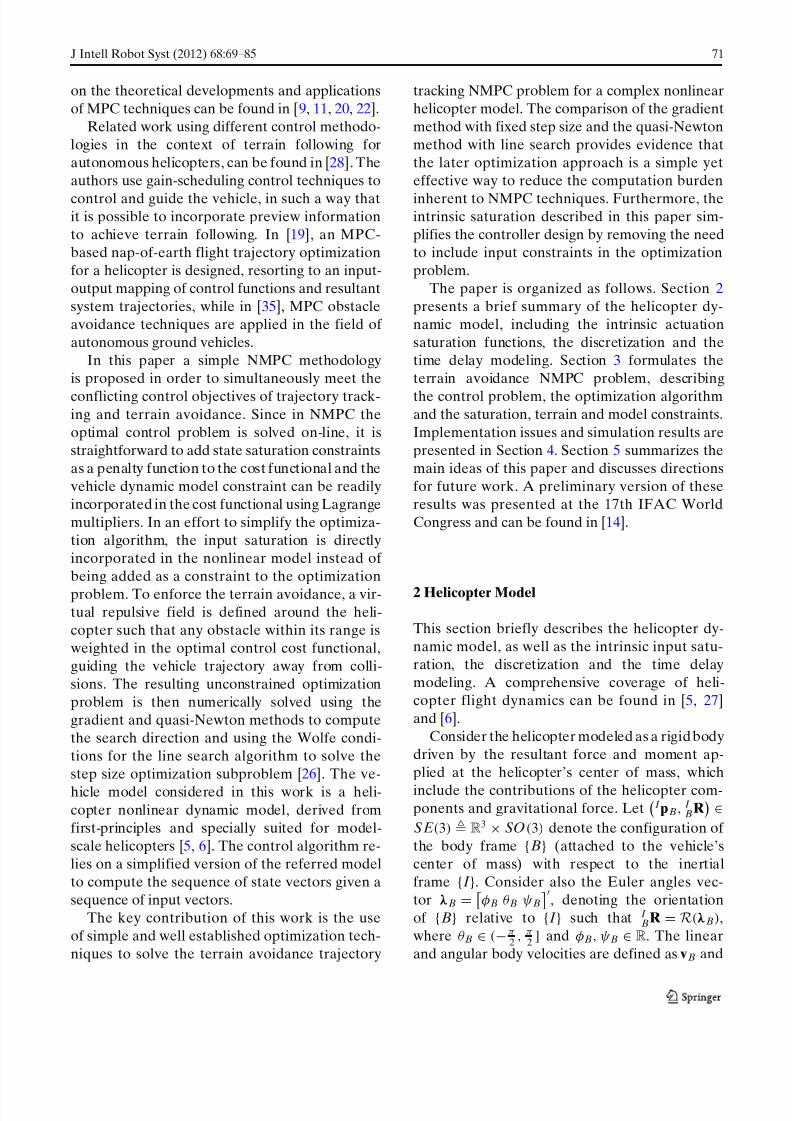
F T (x) = c e− g(x) , (26)

where c > 0 is a scalar weight selected such that,

when g(x) = 0 the respective value of the terrainconstraint, F T (x) = c, is adequate to drive the

vehicle away from the terrain in the foreseen oper-

ation scenarios. The zero value is forced whenever

the distance p is greater than a predefined outer

radius r O where the influence of the terrain is

negligible, that is F T = 0 if p > r O, thus avoid-

ing unnecessary computational burden. Note that

even if this procedure is not performed, the devia-tion from the desired trajectory will be negligible,

since the terms Li of the cost function will always

be dominant when the vehicle is not close to the

terrain. The derivative of this terrain constraint is

computed using

∂ F T

∂x= −2 c p e− g(x),

∂ p

∂x(27)

and

∂ p∂x

=

03×3 03×3 ∂ p∂p

03×3

, (28)

where the derivative ∂ p∂p is computed numerically,

based on the available information of the terrain.

The values used throughout this work for the

constants described earlier are c = 1, r 0 = 10m,

and r S = 5m. An example of a one-dimension ver-

sion of this function can be seen in Fig. 2. This type

of function has the advantage of being defined for

all x ∈ Rn x , while the ubiquitous infinity barrier

type of constraint functions, applied to this safetysphere concept, may lead to problems during ini-

0 2−2 4−4 6−6 8−8 10−100

1

2

3

4

5

6

7

8x 1010

x [m]

0 2−2 4−4 6−6 8−8 10−10

x [m]

F T

( x )

F T

( x )

FT(x)

Safety radius

(a) Global view

0

10

20

30

40

50

60

70

80

90

100

(b) Detail on safety sphere boundary

FT(x)

Safety radius

Fig. 2 One-dimensional function c e− g( x), with g( x) = x2 − 52 and c = 1




tialization or when avoiding the terrain. For in-

stance, for takeoff maneuvers, the vehicle would

be initialized with the terrain inside the safety

sphere and the proposed terrain constraint alone

would drive its trajectory away from the terrain,

whereas the infinity barrier constraint is not co-

herently defined for such a situation and wouldhave the opposite effect of keeping the vehicle

close to the terrain.

3.2 State and Input Saturation Constraint

The saturation constraints defined in Eq. 19 are

included in the optimization problem to comple-

ment the intrinsic input saturation described in

Section 2.3, enabling the definition of mission

specific bounds for the state and input vectors. If

there is no special requirement in terms of actu-

ation there is no need to have input saturations

in the optimization problem, since the physical

constraints will be always satisfied through the

intrinsic saturations. On the other hand, a mission

where the payload includes sensitive equipment

may require all actuation signals to be further con-

strained into a smaller actuation set, thus avoiding

large acceleration maneuvers.

These constraints can be incorporated in the

cost functional as a penalty function, F R(x

,u

),which is zero-valued for x ∈ X and u ∈ U , and

behaves as a quadratic function outside these sets.

Assuming that the feasibility sets for state and

input vectors are given by X =

x ∈ Rn x : x( j )min ≤

x( j ) ≤ x( j )max ∀ j =1,...,n x

and U =

u ∈Rnu : u

(l )min ≤

u(l ) ≤ u(l )max ∀l =1,...,nu

, respectively, the penalty

function can be defined as

F R(x, u) =

n x

j =1

f R( x( j )) +

nu

l =1

f R(u(l )) , (29)

where

f R(a) =1

2h2(|a− acenter| − arange) wa , (30)

wa is a positive scalar weight, acenter = (amax +

amin)/2, arange = amax − acenter, and

h(a) =

a , if a > 0

0 , otherwise. (31)

The derivative of this constraint is computed

analytically using the derivative of the generic

function f R(a), given by

d f R(a)

da= sign(a− acenter)

× h(|a− acenter| − arange) wa . (32)

3.3 Unconstrained Optimization Problem

The unconstrained optimization control problem

can be defined as

U∗k = arg min

Uk

¯ J N ,k (33)

s.t . f M (Xk, Uk) = 0 (34)

where the terrain and saturation constraints are

incorporated in the new cost functional by using

¯ J N ,k = ¯ J N (Xk, Uk) = F k+N +

k+N −1i=k

Li , (35)

F i = F (xi) = F i + F R(xi, 0) + F T (xi) , (36)

Li = L(xi, ui) = Li + F R(xi, ui) + F T (xi) , (37)

and the model constraint 34 is solved by the

elimination method using Lagrange multipliers.Introducing the Lagrange multiplier sequence

k = {λk+1, . . . ,λk+N } and the Hamiltonian H i =

H (xi, ui) = Li + λi+1 f (xi, ui), the cost functional

can be rewritten as

¯ J N ,k = F k+N − λk+N xk+N

+

k+N −1i=k+1

H i − λ

i xi

+ H k. (38)

For a fixed initial state xk, the first order conditionof optimality yields

∂ ¯ J N ,k

∂xi=

∂ H i

∂xi− λ

i = 0 , ∀i=k+1,...,k+N −1 , (39)

∂ ¯ J N ,k

∂xk+N

=∂ F k+N

∂xk+N

− λk+N = 0 , (40)

∂ ¯ J N ,k

∂ i=

∂ H i

∂ui= 0 , ∀i=k,...,k+N −1 , (41)




where ∂ H i∂ui

= ∂ Li∂ui

+ λi+1

∂ f i∂ui

and ∂ H i∂xi

= ∂ Li∂xi

+

λi+1

∂ f i∂xi

. The lagrange multipliers are defined as

λk+N =

∂ F k+N

∂xk+N

and λi =

∂ H i

∂xi, ∀i=k+1,...,k+N −1,

(42)

so that the first order conditions of optimality

reduce to Eq. 41.

An iterative algorithm based on the first order

gradient method can be applied to estimate U∗k,

updating the control sequence at each iteration

according to

Uk ← Uk + sk , (43)

where the step size is denoted by s and the search

direction by k. The optimization algorithm canbe summarized as follows.

Algorithm 1 Minimization algorithm for the

NMPC unconstrained problem.

1. Initialize Xk, Uk;

2. Compute {λi}, i = k+ N , . . . ,k;

3. Compute

∂ H i

∂ui

, i = k, . . . ,k+ N − 1;

4. Compute the search direction k ;

5. Compute the step size s;

6. Compute the new Uk using Eq. 43 and thenew Xk = {xi} using xi+1 = f (xi, ui), for i =

k+ 1, . . . ,k+ N ;

7. Test stop conditions: if false go to step (2),

if true let Uk = Uk be the final estimate, ap-

ply first input vector uk to system and set

the next initial solution to Uk ← {uk+1, . . . ,

uk+N −1, uk+N −1}.

The search direction is denoted by the sequence

k = {δk, . . . , δk+N −1} and can be obtained using

either the gradient or the quasi-Newton methods,given respectively by

δi = −∂ H i

∂uiand δi = −Di

∂ H i

∂ui, (44)

where the matrices Di are estimates for the in-

verse second-order derivatives ∂ 2 H i∂ui∂ui

, computed as

in [26].

The line search optimization subproblem, used

to estimate the optimal step size s∗, is numerically

solved using the Wolfe rule. This approach guar-

antees a decrease of the cost functional, as the well

known Armijo rule does, and ensures reasonable

progress by ruling out unacceptably short steps

[26]. Consider the step size optimization subprob-

lem defined as

s∗ = arg min s≥0

φ ( s) , (45)

where the cost functional is φ ( s) = ¯ J +N ,k =

¯ J N

X+k , U+

k

, with U+

k = Uk + sk, X+k =

X(xk, Uk + sk), and the first order condition of

optimality is given by

d φ ( s)

d s=

d ¯ J +N ,k

d s= 0 . (46)

The superscript (.)+ denotes the result of up-

dating a variable using the step size s. Not-ing that ¯ J N −i,k+i = Lk+i + ¯ J N −i−1,k+i+1 for all i =

0, . . . ,N − 1, the derivatived ¯ J +N ,k

d scan be defined

using

d ¯ J +N −i,k+i

d s=

∂ L+k+i

∂xk+i

ηk+i +∂ L+

k+i

∂uk+i

δk+i

+d ¯ J +N −i−1,k+i+1

d s, (47)

d ¯ J +

0,k+N d s =

∂ F +

k+N ∂xk+N

ηk+N , (48)

ηk+i =d x+

k+i

d s=

∂ f +k+i−1

∂xk+i−1

ηk+i−1

+∂ f +k+i−1

∂uk+i−1

δk+i−1 , (49)

Let also μ1 = φ (0) + σ 1d φ (0)

d ss and μ0 = σ 0

d φ (0)

d s,

where σ 1 and σ 0 are parameters of the search

algorithm. The Wolfe conditions classify a step

size according to the sets

A =

s > 0 : φ ( s) ≤ μ1 ∧

d φ ( s)

d s≥ μ0

D = { s > 0 : φ ( s) > μ1}

E =

s > 0 : φ ( s) ≤ μ1 ∧

d φ ( s)

d s< μ0

, (50)

that define the acceptable, the right unacceptable,

and the left unacceptable step sizes, respectively.

By using a basic search algorithm an acceptable




step size is obtained, yielding an estimate of the

optimal step size.

4 Simulation Results

The terrain avoidance NMPC algorithm pre-sented in this work is designed to provide the

unmanned rotorcraft with low altitude flight capa-

bilities even in operation scenarios where the pre-

defined trajectory collides with the terrain. In this

section the performance of the proposed method

is evaluated in simulation.

Since the problem of terrain acquisition and

representation is not the main focus of this paper,

it is assumed that the terrain is represented by

an elevation function and that this information

enters the control algorithm in the computationof the helicopter-terrain distance. In the results

presented hereafter, the helicopter model de-

scribed in Section 2 is parameterized for the Vario

X-treme model scale helicopter and used to close

the simulation loop [5]. A simplified, yet highly

nonlinear, version of this model is used in the con-

trol algorithm. Full analytical expressions for the

first order derivatives of this model were obtained

in order to efficiently compute the actuation at

each sampling time. Simulations were carried

out in Matlab/Simulink with C mex-functions,using an Intel Core™2 T9550 at 2.66GHz with

3GB of RAM running Ubuntu 10.10 operative

system.

The simulation results presented in this section

are two-fold. Firstly, a terrain avoidance simula-

tion is presented to demonstrate the capabilities

of the algorithms in collision avoidance situations

and to compare the performance of each opti-

mization algorithm. Secondly, a shorter simula-

tion is presented to illustrate particular aspects of

this NMPC, such as the natural previewing ability

of MPC strategies or the activation of intrinsic

saturations and saturation constraints included in

the optimization problem.

4.1 Terrain Avoidance Results

The terrain used in the first simulation resembles

a winding water stream and the reference trajec-

tory comprises three sections: (1) hovering flight

at the initial position; (2) forward flight trajec-

tory with constant speed v = 2 ms−1; and (3)

hovering flight at the final position. The sample

time is T s = 0.02 s and the horizon is N = 50

sample times, or equivalently 1 s. This horizon

is sufficiently large to allow for the algorithm to

predict impacts with the terrain and change thehelicopter trajectory to avoid it. The precision

of the solution is determined by the algorithm

stop condition given by ∇ Uk¯ J N ,k/∇ Uk

¯ J (0)

N ,k <

10−3, where ¯ J (0)

N ,k is the initial value of the cost

functional. Noting that the final state vector is

defined as xk =

vBk

ωBk

pBk

λBk

θ 1k uBk−1

, the

cost functional matrices used in the simulation

results are

R = diag(150, 300, 300, 150) , (51)

Q = diag(I3, 3 I2, 10, 5 I3, I2, 10, I2, R) , (52)

and the P matrix is computed as the steady-

state solution of the discrete-time algebraic

Riccati equation using matrices Q and R, for the

helicopter model linearized around hover. The

operator diag(.) stands for the block diagonal ma-

trix formed by the arguments, and In is the n× n

identity matrix.

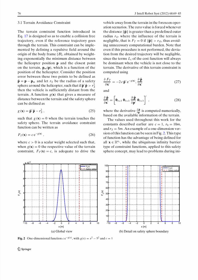
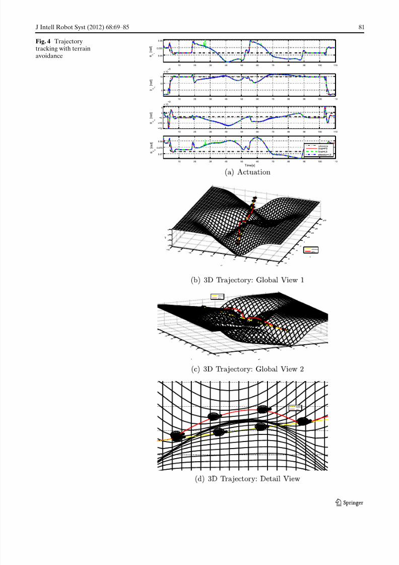
The simulation results presented in Figs. 3and 4, feature the time evolution of the position,

Euler angles, linear velocity, actuation and the

3-D trajectory described by the helicopter. These

results include the values for each of the three op-

timization algorithms: gradient method with fixed

step (Grad-FS), gradient method with line search

(Grad-LS); and quasi-Newton method with line

search (qNewton-LS). For the Grad-FS algorithm,

the value s = 10−6 was chosen for the step size

so that the algorithm converges at each instant

of the desired simulation with a good rate of

convergence. Since the optimization problem and

the termination tolerance are the same for each

of these algorithms, the performance in terms of

minimization of the cost function should be the

same, apart from numerical issues. Note that the

cost function minimization includes several terms:

trajectory following, terrain avoidance, control

effort, and saturations. It can be seen in the sim-

ulation plots that all the variables of the three




Fig. 3 Trajectorytracking with terrainavoidance

10 20 30 40 50 60 70 80 90 100 110

0

50

−50

−100

100

x [ m ]

10 20 30 40 50 60 70 80 90 100 110

0

10

−10

−20

−30

−32

−34

−36

−0.02

−0.06

−0.04

20

y [ m ]

10 20 30 40 50 60 70 80 90 100 110

Time[s]

z [ m ]

reference

10 20 30 40 50 60 70 80 90 100 110

φ [ r a d ]

10 20 30 40 50 60 70 80 90 100 110

0

0.05

−0.05

−0.2

−0.4

−0.6

−0.1

0.1

θ [ r a d ]

10 20 30 40 50 60 70 80 90 100 110

0

Time[s]

ψ

[ r a

d ]

reference

10 20 30 40 50 60 70 80 90 100 110

0

1

2

u [ m / s ]

10 20 30 40 50 60 70 80 90 100 110

0

0.5

1

v [ m / s ]

10 20 30 40 50 60 70 80 90 100 110

0

0.5

−0.5

Time[s]

w

[ m / s ]

reference




Fig. 4 Trajectorytracking with terrainavoidance

10 20 30 40 50 60 70 80 90 100 110

0.05

0.055

0.06

θ c 0

[ r a d ]

10 20 30 40 50 60 70 80 90 100 110

5

10

15

x 10

θ c 1 c

[ r a d ]

10 20 30 40 50 60 70 80 90 100 110

0

5

x 10

θ c 1 s

[ r a d ]

10 20 30 40 50 60 70 80 90 100 110

0.07

0.075

0.08

Time[s]

θ c 0 t

[ r a d ]

reference

0

20

40

60

80

100

020

4060

80100

10

20

30

40

X

reference

MPC

0

20

40

60

80

100

020

4060

X

reference

MPC

reference

MPC




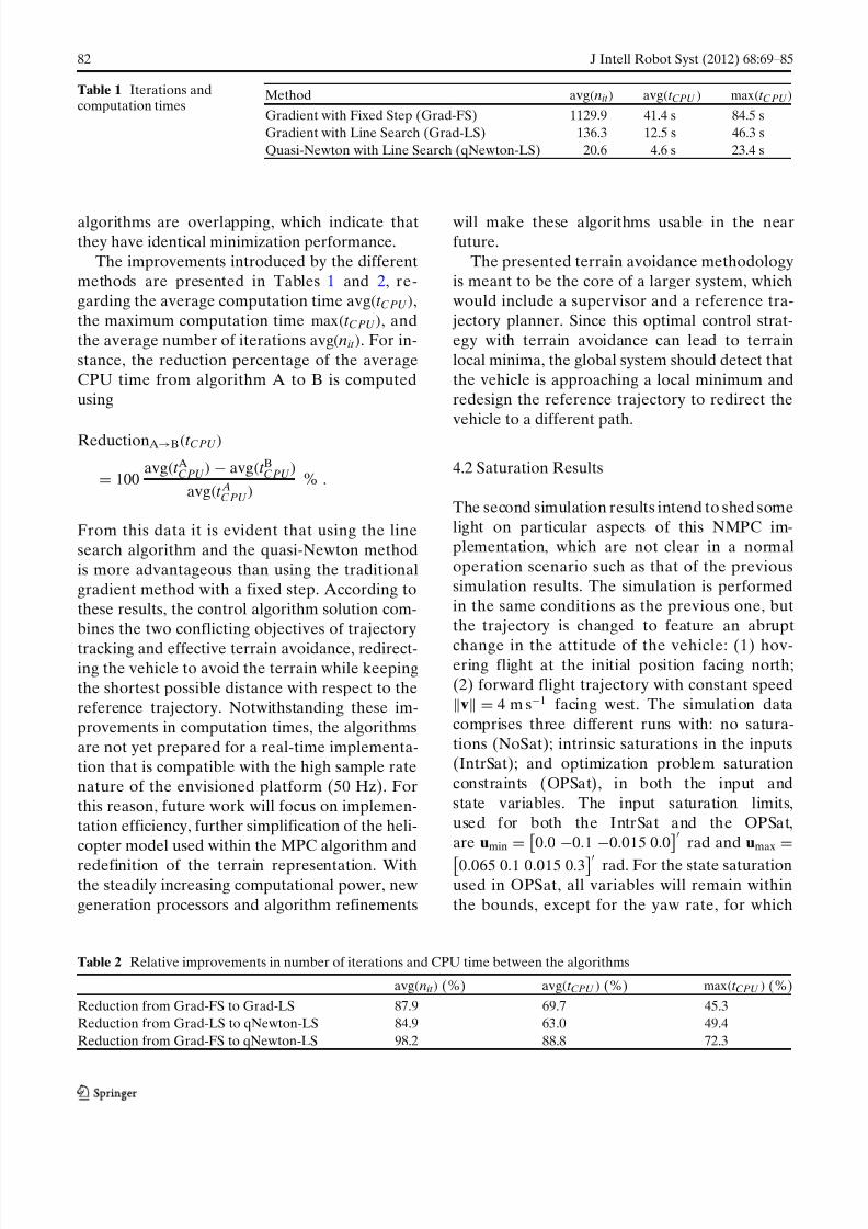
Table 1 Iterations andcomputation times

Method avg(nit ) avg(t CPU ) max(t CPU )

Gradient with Fixed Step (Grad-FS) 1129.9 41.4 s 84.5 s

Gradient with Line Search (Grad-LS) 136.3 12.5 s 46.3 s

Quasi-Newton with Line Search (qNewton-LS) 20.6 4.6 s 23.4 s

algorithms are overlapping, which indicate that

they have identical minimization performance.

The improvements introduced by the different

methods are presented in Tables 1 and 2, re-

garding the average computation time avg(t CPU ),

the maximum computation time max(t CPU ), and

the average number of iterations avg(nit ). For in-

stance, the reduction percentage of the average

CPU time from algorithm A to B is computed

using

ReductionA→B(t CPU )

= 100avg(t ACPU ) − avg(t BCPU )

avg(t ACPU )% .

From this data it is evident that using the line

search algorithm and the quasi-Newton method

is more advantageous than using the traditional

gradient method with a fixed step. According to

these results, the control algorithm solution com-

bines the two conflicting objectives of trajectory

tracking and effective terrain avoidance, redirect-ing the vehicle to avoid the terrain while keeping

the shortest possible distance with respect to the

reference trajectory. Notwithstanding these im-

provements in computation times, the algorithms

are not yet prepared for a real-time implementa-

tion that is compatible with the high sample rate

nature of the envisioned platform (50 Hz). For

this reason, future work will focus on implemen-

tation efficiency, further simplification of the heli-

copter model used within the MPC algorithm and

redefinition of the terrain representation. Withthe steadily increasing computational power, new

generation processors and algorithm refinements

will make these algorithms usable in the near

future.

The presented terrain avoidance methodology

is meant to be the core of a larger system, which

would include a supervisor and a reference tra-

jectory planner. Since this optimal control strat-

egy with terrain avoidance can lead to terrain

local minima, the global system should detect that

the vehicle is approaching a local minimum and

redesign the reference trajectory to redirect the

vehicle to a different path.

4.2 Saturation Results

The second simulation results intend to shed some

light on particular aspects of this NMPC im-

plementation, which are not clear in a normal

operation scenario such as that of the previous

simulation results. The simulation is performed

in the same conditions as the previous one, but

the trajectory is changed to feature an abrupt

change in the attitude of the vehicle: (1) hov-ering flight at the initial position facing north;

(2) forward flight trajectory with constant speed

v = 4 m s−1 facing west. The simulation data

comprises three different runs with: no satura-

tions (NoSat); intrinsic saturations in the inputs

(IntrSat); and optimization problem saturation

constraints (OPSat), in both the input and

state variables. The input saturation limits,

used for both the IntrSat and the OPSat,

are umin = 0.0 −0.1 −0.015 0.0

rad and umax =0.065 0.1 0.015 0.3

rad. For the state saturation

used in OPSat, all variables will remain within

the bounds, except for the yaw rate, for which

Table 2 Relative improvements in number of iterations and CPU time between the algorithms

avg(nit ) (%) avg(t CPU ) (%) max(t CPU ) (%)

Reduction from Grad-FS to Grad-LS 87.9 69.7 45.3

Reduction from Grad-LS to qNewton-LS 84.9 63.0 49.4

Reduction from Grad-FS to qNewton-LS 98.2 88.8 72.3




Fig. 5 Saturation testwith: (i) no saturations(NoSat), (ii) intrinsicsaturations in the inputs(IntrSat), and (iii)optimization problemsaturation constraints(OPSat)

1 2 3 4 5 6 7 8 9 100

1

2

3

4

u [ m / s ]

1 2 3 4 5 6 7 8 9 10

0

0.5

−0.5

−1.5

−1

−0.5

−1.5

−1

v [ m / s

]

1 2 3 4 5 6 7 8 9 10

0

Time[s]

w

[ m / s ]

reference

NoSat

IntrSat

OPSat

1 2 3 4 5 6 7 8 9 10

0

0.1

−0.1

−0.2

−0.3

−0.1

−0.2

−0.2

−0.4

−0.6

−0.8

p [ r a d / s ]

1 2 3 4 5 6 7 8 9 10

0

0.1

q [ r a d / s ]

1 2 3 4 5 6 7 8 9 10

0

Time[s]

r [ r a d / s ]

referenceNoSat

IntrSat

OPSat

1 2 3 4 5 6 7 8 9 10

0.04

0.05

0.06

0.07

θ c 0

[ r a d ]

1 2 3 4 5 6 7 8 9 100.005

0.010.0150.02

0.025

θ

c 1 c

[ r a d ]

1 2 3 4 5 6 7 8 9 10

0

−10

−20

x 10

θ c 1 s

[ r a d ]

1 2 3 4 5 6 7 8 9 100.06

0.08

0.1

Time[s]

θ c 0 t

[ r a d ] reference

NoSat

IntrSat

OPSat




the absolute value is saturated at 0.4 rads−1. The

bounds considered for this simulation results are

more restrictive than the real bounds used in the

terrain avoidance simulation in order to show the

behavior of the saturation strategies. It can be

observed in Fig. 5, that both saturation strategies,

IntrSat and OPSat, are effectively keeping themain rotor collective and lateral cyclic controls

within the bounds. Moreover, the state saturation

in the optimization problem is also constraining

the yaw rate absolute value below 0.4 rads−1. It

can also be seen that the control algorithm starts

changing the control effort N steps ahead of the

change in the reference trajectory, demonstrating

the preview ability of this NMPC strategy.

As discussed above, the objective of having

intrinsic saturations is to make sure that the physi-

cal limitations of the platform and the numericallimitations of the model are always taken into

account in the form of input saturations within

the model function, even if there are no saturation

constraints in the optimization problem.

5 Conclusions

Motivated by the use of autonomous rotorcraft

in low altitude flight applications, this paper pre-

sented a simple NMPC-based strategy for terrainavoidance and motion control of helicopters. In

addition to imposing state and input saturation

constraints, the proposed solution enforces terrain

avoidance by defining a repulsive field around

the helicopter that grows exponentially fast as the

distance between the vehicle and the closest point

on the terrain decreases.

In contrast to the standard approach in NMPC

literature, the actuation constraints were incorpo-

rated into the model so that every control action

provided by the control algorithm is always valid

and the controller design is simplified. The con-

strained optimization problem was reformulated

as an unconstrained optimization problem using

penalty methods to accommodate the saturation

and terrain constraints, and Lagrange multipli-

ers to eliminate the helicopter dynamic model

constraint. The optimization problem was solved

using an iterative algorithm that relies on the

gradient and quasi-Newton methods to find the

search direction and on the Wolfe conditions to

find an estimate of the optimal step size. The

simulation results were obtained using a simplified

nonlinear helicopter model in the MPC algorithm

and the full model as the real plant, showing that

the presented methodology can achieve effective

terrain avoidance while steering the vehicle alonga reference trajectory. Moreover, it is shown that

resorting to the quasi-Newton method with line

search drastically reduced the number of itera-

tions and CPU time relatively to the standard

gradient method with fixed-step.

Similarly to most NMPC strategies used in high

sampling rate platforms, the proposed methodol-

ogy faces the challenge of real time implemen-

tation. Nevertheless, the constant technological

advancements in terms of processing capability

will enable the use of refined versions of thesealgorithms in the near future. In terms of CPU

time consumption, the most critical tasks involve

the helicopter model computations and the algo-

rithm to determine the closest point on the ter-

rain (which with modern sensors, like LADARs

or time-of-flight cameras, can be obtained with

negligible processing). Therefore, future work will

focus on implementation efficiency, simplification

of the helicopter model and also the simplification

of the closest point computation. Furthermore,

future algorithms shall be compared with otherexisting obstacle avoidance methods [12], using a

standard set of benchmarks such as in [24].

References

1. Alamir, M., Bornard, G.: Stability of a truncatedinfinite constrained receding horizon scheme: the gen-eral discrete nonlinear case. Automatica 31(9), 1353–

1356 (1995)2. Bemporad, A., Morari, M., Pistikopoulos, E.N.,Dua, V.: The explicit linear quadratic regulator for con-strained systems. Automatica 38(1), 3–20 (2002)

3. Chen, C.C., Shaw, L.: On receding horizon feedbackcontrol. Automatica 18(3), 349–352 (1982)

4. Chen, H., Allgöwer, F.: A quasi-infinite horizon nonlin-ear model predictive control with guaranteed stability.Automatica 34(10), 1205–1217 (1998)

5. Cunha, R.: Modeling and Control of an AutonomousRobotic Helicopter. Master’s thesis, Department of Electrical and Computer Engineering, Instituto Supe-rior Técnico, Lisbon, Portugal (2002)




6. Cunha, R., Guerreiro, B., Silvestre, C.: Vario-xtremeHelicopter Nonlinear Model: Complete and SimplifiedExpressions. Technical report, Instituto Superior Téc-nico, Institute for Systems and Robotics (2005)

7. Cutler, C.R., Ramaker, B.L.: Dynamic matrix control:a computer control algorithm. In: Proceedings of theJoint Automatic Control Conference. San Francisco,

CA (1980)8. de Nicolao, G., Magnani, L., Magni, L., Scattolini, R.:A stabilizing receding horizon controller for nonlineardiscrete time systems. In: American Control Confer-ence. Chicago, Illinois (2000)

9. Findeisen, R., Imsland, L., Allgöwer, F., Foss, B.A.:State and output feedback nonlinear model predictivecontrol: an overview. Europ. J. Contr. 9, 179–195 (2003)

10. Garcia, C.E., Prett, D.M., Morari, M.: Model predictivecontrol: theory and practice—a survey. Automatica25(3), 335–348 (1989)

11. Garcia, C.E., Morari, M.: Internal model control. Aunifying review and some new results. Ind. Eng. Chem.Process Des. Dev. 21(2), 308–323 (1982)

12. Goerzen, C., Kong, Z., Mettler, B.: A survey of motion planning algorithms from the perspective of autonomous uav guidance. J. Intell. Robot. Syst. 57,65–100 (2010)

13. Grancharova, A., Kocijan, J., Johansen, T.A.: Explicitstochastic predictive control of combustion plantsbased on gaussian process models. Automatica 44,1621–1631 (2008)

14. Guerreiro, B., Silvestre, C., Cunha, R.: Terrain avoid-ance model predictive control for autonomous rotor-craft. In: Proceedings of the 17th IFAC WorldCongress (IFAC’08), pp. 1076–1081. Seoul, Korea(2008)

15. Jadbabaie, A., Yu, J., Hauser, J.: Unconstrainedreceding-horizon control of nonlinear systems. IEEETrans. Automat. Contr. 46(5), 776–783 (2001)

16. Keerthi, S.S., Gilbert, E.G.: Optimal infinite-horizonfeedback laws for a general class of constraineddiscrete-time systems: stability and moving-horizonapproximations. J. Optim. Theory Appl. 57(2), 265–293(1988)

17. Keviczky, T., Balas, G.J.: Receding horizon controlof an f-16 aircraft: a comparative study. Control Eng.Pract. 14(9), 1023–1033 (2006)

18. Kim, H., Shim, D., Sastry, S.: Nonlinear model predic-tive tracking control for rotorcraft-based unmannedaerial vehicles. In: American Control Conference,

vol. 5, pp. 3576–3581. Anchorage, AK (2002)19. Lapp, T., Singh, L.: Model predictive control basedtrajectory optimization for nap-of-earth flight includingobstacle avoidance. In: American Control Conference,pp. 891–892. Boston, MA (2004)

20. Magni, L.: On robust tracking with non-linear modelpredictive control. Int. J. Control 75(6), 399–407 (2002)

21. Magni, L., Raimondo, D.M., Allgöwer, F. (eds.):Nonlinear Model Predictive Control: Towards NewChallenging Applications. Lecture Notes in Controland Information Sciences, vol. 384. Springer, NewYork (2009)

22. Mayne, D., Rawlings, J., Rao, C., Scokaert, P.:Constrained model predictive control: stability andoptimality. Automatica 36, 790–814 (2000). SurveyPaper

23. Mehra, M., Rouhani, R., Eterno, J., Richalet, J., Rault,A.: Model algorithmic control: review and recentdevelopment. In: Proceedings of the Eng. Foundation

Conf. on Chemical Process Control II, pp. 287–310.Sea Island, Georgia (1982)24. Mettler, B., Goerzen, C., Kong, Z., Whalley, M.:

Benchmarking of obstacle field navigation algorithmsfor autonomous helicopters. In: Proceedings of theAmerican Helicopter Society 66th Annual Forum.Phoenix, AZ (2010)

25. Michalska, H., Mayne, D.Q.: Robust receding horizoncontrol of constrained nonlinear systems. IEEE Trans.Automat. Contr. 38(11), 1623–1633 (1993)

26. Nocedal, J., Wright, S.: Numerical Optimization.Springer Series in Operation Reasearch. Springer,New York (1999)

27. Gareth, D., Padfield.: Helicopter Flight Dynamics:

The Theory and Application of Flying Qualities andSimulation Modeling. AIAA Education Series. AIAA,Washington DC (1996)

28. Paulino, N., Silvestre, C., Cunha, R.: Affine parameter-dependent preview control for rotorcraft terrainfollowing. AIAA J. Guid. Contr. Dynam. 29(6),1350–1359 (2006)

29. Propoi, A.I.: Use of linear programming methods forsynthesizing sample-data automatic systems. Autom.Remote Control 24, 837 (1963)

30. Qin, S.J., Badgwell, T.A.: A survey of industrial modelpredictive control technology. Control Eng. Int. 11,733–764 (2003)

31. Rawlings, J.B., Muske, K.R.: The stability of constrained receding horizon control. IEEE Trans.Automat. Contr. 38(10), 1512–1516 (1993)

32. Richalet, J., Rault, A., Testud, J.L., Papon, J.: Modelpredictive heuristic control: applications to industrialprocesses. Automatica 14, 413–428 (1978)

33. Shim, D., Kim, H., Sastry, S.: Decentralized reflectivemodel predictive control of multiple flying robots indynamic environment. In: Conference on Decision andControl, USA (2003)

34. Sutton, G., Bitmead, R.: Computational implemen-tation of nonlinear model predictive control tononlinear submarine. In: Allgöwer, F., Zheng, A.(eds.) Nonlinear Model Predictive Control, Progress in

Systems and Control Theory, pp. 461–471. Birkhäuser,Basel-Boston-Berlin (2000)35. Yoon, Y., Shin, J., Kim, H., Park, Y., Sastry, S.: Model-

predictive active steering and obstacle avoidance forautonomous ground vehicles. Control Eng. Pract. 17,741–750 (2009)

36. Zadeh, L.A., Whalen, B.H.: On optimal control andlinear programming. IRE Trans. Automat. Contr. 7(4),45–46 (1962)

37. Zavala, V.M., Biegler, L.T.: The advanced-stepnmpc controller: optimality, stability, and robustness.Automatica 45(1), 83–93 (2009)

terrain avoidance nonlinear model predictive control for autonomous rotorcraft

Documents