tesis doctoral métodos de clustering en datos de ... · aknowledgements at last, the time of...
TRANSCRIPT

UNIVERSIDAD CARLOS III DE MADRID
TESIS DOCTORAL
Métodos de clustering en datos de expression génica
Autor: Aurora Torrente Orihuela
Directores:
Dr. Alvis Brazma Dr. Juan Romo
DEPARTAMENTO DE ESTADISTICA
Leganés, marzo de 2007


A papa y mama


Aknowledgements
At last, the time of ending up has arrived. And it seems the most difficult part because
compressing in a few words all the gratefulness I feel for all those people that somehow have
been by my side, giving me support, is a hard task...
The first people I want to thank are my parents, my sisters and my best friend Tere, for
having expected from me much more than I ever did, and for being sure all the time that this
end would come.
Next, I want to thank Vıctor Hernandez for introducing me to one of my supervisors, Juan
Romo, for giving me the opportunity to start this work and for believing and supporting my
work at any time. I am also very grateful to Juan, who gave me always the optimism I often
lacked of and for his advices.
I want to specially mention all the colleagues, mates and friends that I have been so lucky
to meet along these years: at the department of Statistics in Leganes, thanks to Marıa, Isaac,
Angel, Juan Carlos, Conchi, Julia and Ismael, and in Getafe, to all those people I’m very
pleased to have met, who were always willing to help: Charo, Esther, Javier, and of course,
Sara, who always was an understanding, supporting friend, and who it’s been a pleasure to
work with.
Next, at the department of Physics, I want to thank Dani (and Maripaz) because of their
friendship and support, and Roberto for his advices. And finally, hundreds of kilometers away,

at my missed EBI, I have to say that I met some incredible people that always were by my
side: above all of them I want to thank my other supervisor, Alvis Brazma. I have no words to
express my gratitude for his constant help, his brilliant ideas, and for having turned my poor
skills and results into pages of work I became proud of. Thank you very much in deed. I also
feel grateful to Misha, who always was patient with me and my problems with unix and EP;
to Jaak, who always had an interesting point of view of my work; to Gabriella, who helped us
with her knowledge about the S.pombe data. And to my friends, Ahmet, who understood and
helped me from the very moment we met, Gonzalo, who invariably reduced the running time of
my algorithms from O(n) to O(ln n); (without him I would still be running my experiments...),
and Marcos, for giving always an optimistic point of view of every problem.
Finally, I want to devote these last lines to the person whose persistence and love made it
possible to end this work. My husband, who never let me surrender or step back during these
years, who made me start alone the amazing experience of my stay abroad, but finish it by
my side, who always tried to make an organized researcher of me (without much success...),
who started me up with LATEX, who always searched for a way out of problems... Too many
things to summarize them all here... Each page in this manuscript is devoted to YOU, (and
specially to the memories from the Cavendish lab and “my” formula... Those were the days of
our lives...). Just thanks...

Indice
Prefacio 1
1. Introduccion 3
1.1. El problema del analisis de conglomerados . . . . . . . . . . . . . . . . . . . . . 4
1.2. Fundamentos de la biologıa molecular . . . . . . . . . . . . . . . . . . . . . . . 12
1.3. Dogma central de la biologıa molecular . . . . . . . . . . . . . . . . . . . . . . . 14
1.4. Microarrays . . . . . . . . . . . . . . . . . . . . . . . . . . . . . . . . . . . . . . 17
1.5. Generacion, procesado y analisis de datos . . . . . . . . . . . . . . . . . . . . . 18
1.6. Fundamentos de la teorıa de grafos . . . . . . . . . . . . . . . . . . . . . . . . . 19
1.7. El principio de la mınima longitud de descripcion . . . . . . . . . . . . . . . . . 21
1.8. Clustering de datos de expresion genica . . . . . . . . . . . . . . . . . . . . . . 25
1.8.1. Medidas de similaridad . . . . . . . . . . . . . . . . . . . . . . . . . . . 26
1.8.2. Criterios del clustering optimo . . . . . . . . . . . . . . . . . . . . . . . 31
1.8.3. Algoritmos de clustering . . . . . . . . . . . . . . . . . . . . . . . . . . . 32
1.9. Problemas abiertos relacionados con el clustering . . . . . . . . . . . . . . . . . 39
i

ii INDICE
1.9.1. Comparacion de dos particiones distintas . . . . . . . . . . . . . . . . . 39
1.9.2. Refinamiento del estado inicial de los metodos de clusterings iterativos . 41
1.9.3. Determinacion del verdadero numero de grupos . . . . . . . . . . . . . . 42
2. Comparacion de resultados de clustering 45
2.1. Introduccion . . . . . . . . . . . . . . . . . . . . . . . . . . . . . . . . . . . . . . 46
2.2. Comparacion de dos clusterings planos . . . . . . . . . . . . . . . . . . . . . . . 49
2.2.1. Union de conglomerados. El algoritmo “greedy” . . . . . . . . . . . . . . 55
2.2.2. Resultados . . . . . . . . . . . . . . . . . . . . . . . . . . . . . . . . . . 61
2.3. Comparacion de un clustering jerarquico y uno plano . . . . . . . . . . . . . . . 63
2.3.1. Funcion de puntuacion basada en Teorıa de la Informacion . . . . . . . 67
2.3.2. Funcion de puntuacion basada en la estetica de la representacion del grafo 71
2.3.3. El algoritmo con exploracion . . . . . . . . . . . . . . . . . . . . . . . . 74
2.4. Resultados . . . . . . . . . . . . . . . . . . . . . . . . . . . . . . . . . . . . . . . 78
2.4.1. Resultados en datos simulados . . . . . . . . . . . . . . . . . . . . . . . 78
2.4.2. Resultados en datos reales . . . . . . . . . . . . . . . . . . . . . . . . . . 87
2.5. Implementacion en Expression Profiler . . . . . . . . . . . . . . . . . . . . . . . 89
3. Refinamientos robustos de k-medias mediante profundidad 91
3.1. Introduccion . . . . . . . . . . . . . . . . . . . . . . . . . . . . . . . . . . . . . . 92
3.2. Metodos . . . . . . . . . . . . . . . . . . . . . . . . . . . . . . . . . . . . . . . . 96
3.2.1. Un calculo eficiente de la profundidad por bandas generalizada . . . . . 96
3.2.2. Alternancia de k-medias con la busqueda de datos mas profundos . . . . 98
ii

INDICE iii
3.2.3. Combinacion de bootstrap con la busqueda de datos mas profundos . . 100
3.3. Resultados . . . . . . . . . . . . . . . . . . . . . . . . . . . . . . . . . . . . . . . 104
3.3.1. Resultados en datos simulados . . . . . . . . . . . . . . . . . . . . . . . 104
3.3.2. Resultados en datos reales . . . . . . . . . . . . . . . . . . . . . . . . . . 117
3.4. Clustering no rıgido basado en bootstrap . . . . . . . . . . . . . . . . . . . . . . 121
3.4.1. Resultados en los datos de leucemia . . . . . . . . . . . . . . . . . . . . 130
4. Estimacion del numero de grupos 133
4.1. Introduccion . . . . . . . . . . . . . . . . . . . . . . . . . . . . . . . . . . . . . . 134
4.2. Comparacion de pares de clusterings . . . . . . . . . . . . . . . . . . . . . . . . 137
4.2.1. Muestreo en una poblacion de clusterings . . . . . . . . . . . . . . . . . 144
4.2.2. Metodo de muestreo de clusterings . . . . . . . . . . . . . . . . . . . . . 149
4.3. Metodo del diametro de los puntos mas profundos . . . . . . . . . . . . . . . . 152
4.4. Resultados . . . . . . . . . . . . . . . . . . . . . . . . . . . . . . . . . . . . . . . 155
4.4.1. Datos simulados . . . . . . . . . . . . . . . . . . . . . . . . . . . . . . . 155
4.4.2. Datos reales . . . . . . . . . . . . . . . . . . . . . . . . . . . . . . . . . . 166
5. Conclusiones y lıneas de investigacion futuras 171
5.1. Conclusiones . . . . . . . . . . . . . . . . . . . . . . . . . . . . . . . . . . . . . 172
5.2. Lıneas de investigacion futuras . . . . . . . . . . . . . . . . . . . . . . . . . . . 174
5.2.1. Comparacion de dos clusterings jerarquicos . . . . . . . . . . . . . . . . 174
5.2.2. Comparacion de un clustering plano y Gene Ontology . . . . . . . . . . 175
iii

iv INDICE
5.2.3. Comparacion de un clustering jerarquico con un conjunto de genes pre-
definido . . . . . . . . . . . . . . . . . . . . . . . . . . . . . . . . . . . . 175
5.2.4. Comparacion de clusterings no rıgidos . . . . . . . . . . . . . . . . . . . 175
Apendice 177
El algoritmo correspondence con exploracion (“look-ahead”) . . . . . . . . 177
Referencias 183
iv

Preface
Clustering is an old data analysis problem that has been extensively studied during
the last decades. However, there is not a single algorithm that provides a satisfactory result
for every data set. Moreover, there exist some problems related to cluster analysis that also
remain unsolved. In this monograph we study some of such problems as they commonly appear
in practice, and test how they work when applied to gene expression data analysis, where
clustering is widely used.
Different clustering algorithms often lead to different results, and in order to make sense
out of them it is important to understand how clusters from one analysis relate to those from a
different one. A comparison method to find and visualize many-to-many relationships between
two clusterings, either two flat clusterings or a flat and a hierarchical clustering, is presented.
The similarities between clusters are represented by a weighted bipartite graph, where the
nodes are the clusters and an edge weight shows the number of elements in common to the
connected nodes. To visualize the relationships between clusterings the number of edge crossings
is minimized. When applied to the case of comparing a hierarchical and a flat clustering we use
a criterion based either on the graph layout aesthetics or in the mutual information, to decide
where to cut the hierarchical tree.
Since iterative methods are sensitive to the initial parameters, we have developed two
refinement algorithms designed to improve this initial state, based on the notion of data depth.
One of these algorithms looks for initial points in the same data space, while the second one,
using the bootstrap technique, selects the initial seeds in a new space of bootstrap centroids.
1

2 PREFACE
Also, this second approach allows to construct a soft (non-hard) clustering of the data, that
assigns to each point a probability of belonging to each cluster, and thus a single point may
partially belong to more than one cluster.
On the other hand, the number of clusters underlying in a data set is usually unknown.
Using ideas from the clustering comparison method previously proposed and from the data
depth concept, we present three procedures to estimate the number of real groups. The first two
methods consist basically in sampling pairs of clusterings from a population and successively
performing comparisons between them to find a consensus in the number of clusters, and the
third one looks for representative subsets of the clusters whose diameter is used to estimate
the optimal number of real groups.
The extensive study we carried out in simulated and real gene expression data shows that
the techniques presented here are useful and efficient. The results that we obtained with real
data make sense not only from a statistical point of view, but they have proven to have a
biological meaning.
2

Chapter 1
Introduction
Summary
Clustering is an old data analysis problem whose aim is the partitioning of a data set into
subsets (clusters) highly internally homogenous (members are similar to one another) and
highly externally heterogenous (members are not like members of other clusters). The interest
in this technique has been recently revived with the use of new methodologies for the study of
gene expression data, such as microarrays. For the understanding of the nature of this type of
data, some basics of molecular biology and a short description of how microarrays are built and
how gene expression data are produced are needed. We summarize some of the features common
to all cluster algorithms, which can be either hierarchical or non-hierarchical (flat): similarity
measures, clustering criteria and algorithms themselves. Finally, we present some of the open
problems related with clustering analysis that are studied in this work: the comparison of two
different clusterings, either hierarchical or flat, the refinement of the initial state of iterative
methods and the estimation of the number of clusters.
3

4 Chapter 1. Introduction
1.1. The clustering problem
Classification of a set of observations or entities into groups is an old data analysis problem.
In Statistics, it is an inherently multivariate problem, whose most common scenario is one in
which the data on hand pertain to many variables measured on each entity and not one involving
just a single variable. This high-dimensional nature of classification provides an opportunity
but also presents some difficulties to the developer of appropriate statistical methodology.
One can distinguish two broad categories of classification problems. In the first, one has
data from known or prespecifiable groups as well as observations from entities whose group
membership, in terms of the known groups, is unknown initially and has to be determined
through the analysis of the data. In the pattern recognition literature this type of classification
problem is referred to as supervised learning; in statistical terminology it falls under the heading
of discriminant analysis. See Ripley and Hjort (1996), for example, as a reference.
On the other hand there are classification problems where the groups are themselves un-
known a priori and the primary purpose of the data analysis is to determine the groupings
from the data themselves, so that the entities within the same group are in some sense more
similar than those that belong to different groups. This type of classification problem is referred
to as unsupervised learning, and in statistical terminology falls under the heading of cluster
analysis.
If one were to consider classification problems in three stages, input, algorithms and output,
it would be fair to say that the vast majority of the work has focused on the second of these.
However, it is clear that a careful thought about what variables to use and how to characterize
and summarize them as inputs to methods of classification are very important issues that
would involve both statistical and subject matter consideration in applications. And similarly,
the most challenging aspect of most analyses of data tends not to be the choice of a particular
method but the interpretation of the output and results of algorithms.
The discriminant analysis situation has been a more integral part of the historical develop-
4

1.1 The clustering problem 5
ment of multivariate statistics, although the cluster analysis case received most of its impetus
from fields such as psychology and biology until relatively recently, being nowadays used in
many fields including machine learning, data mining, pattern recognition, image analysis and
bioinformatics. In part, the historical lack of statistical emphasis in cluster analysis may be due
to the greater inherent difficult of the technical problems associated with it. Even a precise and
generally agreed upon definition of a cluster is hard to come by. The data-dependent nature of
the clusters, the number of them and their composition appear to cause fundamental difficul-
ties for formal statistical inference and distribution theory. Except for ad hoc algorithms for
carrying out cluster analysis themselves, counterparts of many other statistical methods that
exist for the discriminant analysis cases are unavailable for the cluster analysis situation. In
this work we have focused on this second category of classification.
Cluster analysis is a common technique for statistical data analysis. It searches through
data for observations that are similar enough to each other to be usefully identified as part of
a common cluster, what is a very intuitive and natural objective. More precisely, it intends to
combine observations into groups or clusters such that:
1. Each cluster is homogeneous or compact with respect to certain characteristics;
that is, observations in each group are similar to each other.
2. Each group should be different from other groups with respect to the same charac-
teristics; that is, observations of one group should be different from the observations
of other groups.
Rudimentary, exploratory procedures are often quite helpful in understanding the complex
nature of multivariate relationships, and searching the data for a structure of natural groupings
or clusters is an important example of such techniques. If each observation is identified with one
and only one cluster, then the clusters constitute a partition of the data that can be very useful
for statistical purposes. For instance, it is often possible to summarize a large multivariate data
5

6 Chapter 1. Introduction
set in terms of a “typical” member of each cluster and this would be more meaningful that only
looking at a single “typical” member of the entire data and much more concise than individual
descriptions of each observation. Another use occurs when one is attempting to model data
in the presence of cluster structure. Better results may be achieved by taking this structure
into account before attempting to estimate any of the relationships that may be present. In
general, cluster analysis can provide an informal means for assessing dimensionality, identifying
outliers or suggesting interesting hypothesis concerning relationships. Besides the term cluster
analysis there are a number of terms with similar meanings, including data clustering (or just
clustering), automatic classification, numerical taxonomy, botryology and typological analysis.
Geometrically, the concept of cluster analysis is very simple. Each data can be represented
as a point in a d-dimensional space, where d is the number of variables or characteristics used to
describe the subjects. Cluster analysis groups observations such that each group observations
are similar with respect to the clustering variables. However, graphical procedures for identify-
ing clusters may not be feasible when we have many observations or when we have more than
three variables or characteristics. What is needed, in such a case, is an analytical technique
for identifying groups or clusters of points in a given dimensional space. If grouping is done
on the basis of similarities or distances (dissimilarities) then the inputs required are similarity
measures or data from which similarities can be computed. Cluster analysis is a heuristic tech-
nique; therefore a clustering solution or grouping will result even when there may not be any
natural groups or clusters in the data, and establishing the reliability and external validity of
a cluster solution is very important.
The first step in cluster analysis is to select a measure of similarity (or distance), but the
definition of similarity or homogeneity varies from analysis to analysis and depends on the
objectives of the study. A simple measure is Manhattan distance, equal to the sum of absolute
distances for each variable. The name comes from the fact that in a two-variable case, the
variables can be plotted on a grid that can be compared to city streets, and the distance
6

1.1 The clustering problem 7
between two points is the number of blocks a person would walk. However, a more common
measure is Euclidean distance, computed by finding the square of the distance between each
variable, summing the squares, and finding the square root of that sum. In the two-variable
case, the distance is analogous to finding the length of the hypotenuse in a triangle; that is, it
is the distance “as the crow flies”. A review of cluster analysis in health psychology research
(Clatworthy et al., 2005) found that the most common distance measure in published studies
in that research area is the Euclidean distance or the squared Euclidean distance.
Once a distance measure is selected, elements in the data set can be combined and then
a decision is made on the type of clustering technique to be used and on the particular clus-
tering method. In general, data clustering algorithms can be hierarchical or non-hierarchical
(also called flat or partitional). Hierarchical algorithms find successive clusters using previously
established clusters, whereas flat algorithms determine all clusters at once. Hierarchical algo-
rithms can be agglomerative, starting with each element as a separate cluster and merging
them in successively larger clusters, or divisive, starting with the whole set and dividing it into
successively finer clusters, to form a hierarchy that is traditionally represented as a tree data
structure (called a dendrogram) with individual elements at one end and a single cluster with
every element at the other. Cutting the tree at a given height will give a flat clustering at a
selected precision. Some other examples of partitional clustering are k-means or fuzzy c-means.
The k-means algorithm (MacQueen, 1967) assigns each point to the cluster whose center
(also called centroid) is nearest. The center is the average of all the points in the cluster – that
is, its coordinates are the arithmetic mean for each dimension separately over all the points in
the cluster. The main advantages of this algorithm are its simplicity and speed, which allows
it to run on large datasets. Its disadvantage is that it does not yield the same result with
each run, since the resulting clusters depend on the initial random assignments. It maximizes
inter-cluster (or minimizes intra-cluster) variance, but does not ensure that the result has a
global minimum variance.
7

8 Chapter 1. Introduction
In soft clustering, each point has a degree of belongingness to the clusters rather than
belonging completely to just one cluster. Thus, points on the edge of a cluster, may be in the
cluster to a lesser degree than points in the center of the cluster. For each point x we have
a coefficient giving the degree of being in the k-th cluster uk(x). Usually, the sum of those
coefficients is defined to be 1, so that uk(x) denotes a probability of belonging to a certain
cluster. With the fuzzy c-means algorithm, introduced in Bezdek (1981), the centroid ck of the
k-th cluster is the mean of all points in that cluster, weighted by their degree of belongingness to
the cluster. The algorithm minimizes intra-cluster variance as well, but has the same problems
as k-means: the minimum is a local minimum and the results depend on the initial choice of
weights.
A recent approach to clustering that has attracted a lot of attention is the spectral cluster-
ing, which usually involves taking the top eigenvectors of some (affinity) matrix Sij , based on
a measure of the similarity between point i and j, and using them to cluster the points. Some-
times such techniques are also used to perform dimensionality reduction for clustering in fewer
dimensions. Its ability to identify non convex clusters makes it ideal for a number of applica-
tions, including bioinformatics (Pentney and Meila, 2005), software clustering (Shokoufandeh
et al., 2002, 2005), image segmentation (Shi and Malik, 2000) and speech recognition (Bach
and Jordan, 2005; Brown and Cooke, 1994). For example, the Shi-Malik algorithm (Shi and
Malik, 2000) partitions points into two sets (S1, S2) based on the eigenvector v corresponding
to the second-smallest eigenvalue of the Laplacian L = I − D1/2SD1/2 of S, where D is the
diagonal matrix Dii =∑
j Sij . The algorithm can be used for hierarchical clustering, by repeat-
edly partitioning the subsets. A related algorithm is the Meila-Shi algorithm (Meila and Shi,
2001), which takes the eigenvectors corresponding to the k largest eigenvalues of the matrix
P = SD − 1 for some k, and then invokes another algorithm (e.g. k-means) to cluster points
by their respective k components in these eigenvectors. For a review of spectral clustering and
the main results in the literature see for example Verma and Meila (2003).
8

1.1 The clustering problem 9
The last step in cluster analysis is the decision regarding the number of clusters and finally,
the cluster solution is interpreted. Notice that statistical theory cannot provide a complete
theory of classification. We cannot say how similarities should be judged, though we can give
technical assistance in constructing distances, for example. One general model is that the data is
a random sample from some population with a probability distribution P . A technique produces
some clusters in the sample. A theoretical model generates some clusters in the population with
the distribution P . We evaluate the technique by asking how well the sample clusters agree
with the population clusters.
The proliferation of clustering techniques over the past has demanded the development of
ways of measuring the similarity between two clusterings, to compare how well different data
clustering algorithms perform. There have been several suggestions, the most popular ones
being the Rand index (Rand, 1971) and confusion matrices that summarize overlappings of
clusters.
Another important question in cluster analysis is how many clusters should be sought in
the data set. There is a lot of work in this direction, but the problem is still open. Some of the
techniques used to determine the number of groups are Akaike’s information criterion (Akaike,
1974) or the minimum description length criterion (Rissanen, 1978).
Though clustering is an old data analysis problem, microarray experiments, a revolutionary
high-throughput tool for the study of gene expression, have revived the interest in cluster
analysis by raising new methodological and computational challenges. The size of data bases
that store genome related information increases exponentially and techniques for mining such a
huge amount of data are essential in current research. The need to sort genes into groups based
on some notion of similarity is present in all current genome-wide biological investigations. The
hope is that similarity with respect to a measurable quantity, such as gene expression, is often
indicative of similarity with respect to more fundamental qualities, such as function.
Cluster analysis techniques are extremely useful for grouping genes. Since Eisen et al. (1998)
9
10 Chapter 1. Introduction
published their landmark paper describing cluster analysis of gene expression data in the bud-
ding yeast Schizosaccharomyces cerevisiae, this analytical approach has become a standard for
the analysis of DNA microarray data.
Though in the present work we have exclusively used real data from the field of molecular
biology, this is not the only one where cluster analysis has a huge application. As interesting
examples consider:
Marketing research: Cluster analysis is widely used in market research when working with
multivariate data from surveys and test panels. Market researchers use cluster analysis to
partition the general population of consumers into market segments and to better understand
the relationships between different groups of consumers/potential customers.
Social network analysis: In the study of social networks, clustering may be used to recognize
communities within large groups of people.
Image segmentation: Clustering can be used to divide a digital image into distinct regions for
border detection or object recognition.
Data mining : Many data mining applications involve partitioning data items into related sub-
sets; the marketing applications discussed above represent some examples. Another common
application is the division of documents, such as World Wide Web pages, into genres.
This thesis is organized as follows. Chapter 1 is a general review of cluster analysis techniques
and clustering related problems. In order to understand the nature of the real data we will be
dealing with, we will describe briefly some basics of molecular biology (sections 1.2 and 1.3),
and will explain how the technique of microarrays allows to obtain this data (sections 1.4
and 1.5). Some basics about graph theory and the Minimum Description Length principle,
needed for the understanding of the methods presented here, are described in sections 1.6 and
1.7, respectively, while the basic features about clustering are summarized in section 1.8. The
open-related problems depicted in section 1.9 include the comparison between clusters, the
10

1.1 The clustering problem 11
refinement of iterative clustering methods that depend on the initial selection of parameters
(e.g. k-means) and the choice of an appropriate number of clusters.
Each of these problems is addressed in a different chapter. In chapter 2 we propose a clus-
tering comparison method and its implementation that finds a many-to-many correspondence
between groups of clusters from two clusterings, either flat versus flat or flat versus hierarchical.
In section 2.2 we use a weighted bipartite graph to represent the clusters from two flat cluster-
ings and visualize the correspondences between them by minimizing the number of crossings in
this bi-graph. The greedy algorithm used to merge clusters and to determine a correspondence
between clusters from two flat clusterings is described in section 2.2.1. In section 2.3 we analyze
the problem of comparing a flat and a hierarchical clusterings. We propose an algorithm that
finds the optimal cut-off points in the dendrogram as this is explored first depth. To decide
whether or not we cut further ahead in the dendrogram we use two different scores. In section
2.3.1 we describe the first one, based on information theory concepts and on the Minimum
Description Length principle. In section 2.3.2 we use a score based on the layout aesthetics of
the bi-graph representing both clusterings.
In chapter 3 we describe two methods to refine the initial state of k-means, both using
a generalization of the univariate median (so-called data depth), which is more robust than
the multivariate mean. The definition of data depth that we use, described in Lopez-Pintado
and Romo (2006), has the advantage of having low computational cost, as shown in section
3.2.1. In section 3.2.2 we use a simple approach, alternating the computation of the deepest
point in each cluster with k-means. In section 3.2.3 we sample the data via bootstrap to obtain
different versions of the data set that are clustered to finally combine information from all of
them. This second method can also be used to construct a soft (non-hard) clustering technique,
as explained in section 3.4.
In chapter 4 we use ideas from the previous chapters to develop two methods that estimate
the number of clusters underlying in a data set. The first one is a clustering sampling method
11

12 Chapter 1. Introduction
and it is described in section 4.2.2. The basic idea is to perform successive comparisons of pairs
of flat clusterings, run on the same data set. Depending on whether we compare clusterings
with the same or with a different number of initial clusters we define two approaches, the single
k and the mixed k, respectively. The second one, described in section 4.3, is based on finding
the most representative points of the clusters obtained by some clustering algorithm, using
a notion of data depth, and selecting the number of clusters that minimizes the sum of the
diameters of the subsets thus obtained.
Finally, in chapter 5 we summarize the main findings contained in this thesis and enume-
rate some of the possible research lines derived from this work, like the comparison of two
hierarchical clusterings or two soft clusterings.
1.2. Basics of molecular biology
Since the DNA structure was discovered in 1953 by James Watson and Francis Crick, the
genomic field has experienced an enormous development, and it is widely believed that the
thousands of genes and their products (RNA and proteins) in a given living organism work in
a complicated way.
Figure 1.1: Growth of the ArrayExpress database from October 2003 to September 2004.
In the past several years, a new technology called DNA microarray has attracted a great
interest among researchers of different fields, such as biologists or statisticians, because it
12

1.2 Basics of molecular biology 13
allows to monitor the whole genome of any organism on a single chip, so that we can have
a good picture of the interactions among thousands of genes simultaneously. The potential of
such technology for functional genomics is tremendous, as measuring gene expression levels in
different developmental stages, different body tissues, different clinical conditions and different
organisms is instrumental in understanding gene functions, gene networks or effects of medical
treatments. They have led to the creation of data bases that store genetic information, and it is
quite remarkable that their size grows exponentially. As an example, figure 1.1 represents the
number of hybridizations submitted to ArrayExpress (http://www.ebi.ac.uk/arrayexpress/)
from October 2003 to September 2004. Thus, finding relevant facts in those enormous data
bases and analyzing them is essential in the Biology of this new century.
Figure 1.2: Francis Crick shows James Watson the model of DNA in their room number 103 ofthe Austin Wing at the Cavendish Laboratory, Cambridge, UK.
A key step in the analysis of gene expression data is the identification of groups of genes that
manifest similar expression patterns over several conditions, whose corresponding algorithmic
problem is to cluster multi-condition gene expression patterns. Clustering is one of the most
13
14 Chapter 1. Introduction
widely used methods in gene expression data analysis, which has revived interest in cluster
analysis by raising new computational challenges.
Gene expression data is often described by a matrix with thousands of rows –representing
genes– and maybe hundreds of columns –representing conditions or samples– and it is important
to reduce the dimensionality of this data to understand the structure of the data and the
biological information contained in it. One of the main goals of clustering methods is to discover
similar profiles in the behavior of genes and represent this large amount of data by a few number
of groups with similarly behaving genes.
1.3. Central dogma of molecular biology
Living organisms are complex systems. Hundreds of thousands of proteins exist inside each of
them to help carry out daily functions. These proteins are produced locally, assembled to exact
specifications. The enormous amount of information required to manage this complex system
correctly is stored in the nucleic acids, very large molecules with two main parts: a backbone
of sugar and phosphate and attached molecules called nucleotide bases. There are only four
different nucleotide bases within each nucleic acid (but each one contains millions of bases).
The order in which these nucleotide bases appear in the nucleic acid codes for the information
carried in the molecule. Thus, a strand of nucleic acid can be described mathematically as a
(very long) word constructed over an alphabet A of four letters.
The Desoxiribo-Nucleic Acid (DNA) stores the genetic information. Its bases are adenine
(A), cytosine (C), guanine (G) and thymine (T), and therefore A = {A, C,G, T}. It is a double
stranded molecule formed by complementary pairs: adenine always bonds to thymine (and vice
versa) and guanine always bonds to cytosine (and vice versa). The whole DNA stored in the
cells is called the “genome”.
The other nucleic acid involved in the production of proteins is the Ribo-Nucleic Acid (RNA),
a single-stranded molecule that contains the bases adenine, cytosine, guanine and, instead of
14

1.3 Central dogma of molecular biology 15
Figure 1.3: Structure of a DNA molecule.
thymine, uracil (U). Here, the alphabet is A′ = {A,C, G, U}. It serves as a genetic messenger,
carrying the information contained in the DNA to the parts of the cell where it is used to build
proteins.
Three different processes are responsible for the inheritance of genetic information:
Replication: the double-stranded DNA is duplicated to give identical copies. This
process perpetuates the genetic information.
Transcription: a DNA segment that constitutes a gene (the basic unit of heredi-
tary material: an ordered sequence of nucleotide bases that encodes a product, or a
“meaningful” word from A) is read and transcribed into a single stranded sequence
of RNA.
Translation: the RNA sequence is translated into a sequence of amino acids, the
building blocks of proteins, as these are formed. During translation, three bases
are read at a time from the RNA and translated into one amino acid. (The amino
acids are the letters of the alphabet used to describe proteins.)
The central dogma of molecular biology, first enunciated by Crick in 1958, states that the
15

16 Chapter 1. Introduction
Figure 1.4: The central dogma of the molecular biology “deals with the detailed residue-by-residue transfer of sequential information. It states that such information cannot be transferredfrom protein to either protein or nucleic acid”. In other words, once information gets into proteinit cannot flow back to nucleic acid.
flow of genetic information travels from DNA to RNA, and finally to the translation of proteins,
but not the other way around.
Unfortunatelly, knowing the whole sequence of a particular genome is not enough to under-
stand how genes work (which ones are their functions), how proteins are built up, how cells
conform organisms or what fails when certain malady develops. Therefore, the funtional ge-
nomics tries not only to identify the genome sequence (the whole ensemble of words fromA that
encode the genetic information) but to learn the genes functions and relationships (understand
the “meaning” of these words).
16

1.4 Microarrays 17
1.4. Microarrays
Microarrays were first used to study global gene expresion in 1997 (DeRisi et al., 1997). A
microarray is a slide onto which DNA molecules are attached at fixed locations called spots.
There may be tens of thousands of spots on an array, each containing tens of millions of identical
DNA molecules. For gene expression studies, each of these molecules should identify a single
RNA molecule in a genome.
�����������
����������
�� ��� ������������
���������
Figure 1.5: Construction of a microarray.
The most popular application of microarrays is to compare the gene expression levels in
two different samples (e.g. the same cell type under two different conditions). This is based on
labelling the RNA extracted from each of the samples in two different ways (for example, a
green label for the sample from condition 1 and a red label for condition 2). Both extracts are
incubated with the microarray; labelled gene products bind to their complementary sequence
while non-bound samples are removed by washing. The hybridized microarray is excited by
a laser and scanned to detect the red and green dyes. The amount of fluorescence emitted
upon laser excitation corresponds to the amount of RNA bound to each spot. If the RNA from
condition 1 is in abundance, the spot will be green; if the RNA from condition 2 is in abundance
the spot will be red. If both are equal the spot will be yellow and if neither are present it will
appear black. Thus, from the fluorescence intensities and colours for each spot, the relative
expresion levels of the genes in both samples can be estimated. In this way, thousands of data
17

18 Chapter 1. Introduction
points, each providing information about the expression of a particular DNA transcript, can
be obtained from a single experiment.
1.5. Data generation, processing and analysis
The raw data that is produced from microarray experiments are digital images that are
analysed to obtain information about the gene expression levels. Each spot has to be identified
and its intensity measured and compared to values representing the background, but this is
not a trivial task and it is important to know the principles of image analysis for a better
understanding of the limitations of microarray data.
The first step to process the data is to construct a spot quantitation matrix, where each
row corresponds to one spot on the array and each column represents different quantitative
characteristics of the spot (the total intensity of the spot, the mean, median or mode of the
pixel intensity distribution, the local background, the standard deviation of both signal and
background, etc.).
The data from multiple hybridizations must be transformed and organised in a gene ex-
pression matrix, where each row represents a gene and each column represents an experimental
condition. Obtaining such a matrix is not either a trivial task: for example, a single gene can be
represented by several spots on the array or the same experimental condition can be monitored
in multiple hybridizations carried out over replicated experiments. All the quantities relating
to a gene have to be combined to obtain a single number. Moreover, measurements obtained
using different arrays have to be normalized to make them directly comparable. Because nor-
malization changes the data, one has to understand the principles of the technique used and
how it changes the data. Furthermore, all normalization strategies (total intensity, mean log
centring, linear regression, lowess...) are based on some underlying assumptions regarding the
data and consequently, the normalization approach must be appropriate to the experimental
conditions that are used. There is no standard best method for microarray data normalization
18

1.6 Graph theory basics 19
fitting all cases, and new methods are being developed (see, for example, Bolstad et al. (2003);
Cheng and Li (2005)). After the gene expression data matrix has been generated, we can begin
analysing and mining it.
Microarray technology is still developing rapidly, so it is natural that there are no established
standards for microarray experiments or for processing the raw data. In the absence of such
standards, the Microarray Gene Expression Data (MGED) society (http://www.mged.org/)
has developed recommendations for the minimum information needed about a microarray ex-
periment, that attempts to define the set of information sufficient to interpret the experiments
and the results of the experiment unambiguously, and to enable verification of the data (Brazma
et al., 2001).
1.6. Graph theory basics
Configuration of nodes and connections occur in a great variety of applications. They may
represent physical networks (circuits) or organic molecules, or can be used to represent less
tangible interactions, as may occur in sociological relationships or databases. Formally, such
configurations are modelled by combinatorial structures called graphs. Graph theory defines a
graph G = {N,E} as a set of nodes N (or vertices) and a set of edges E, each of which joins
two nodes –called its endpoints. The nodes and edges may have additional attributes, such as
colour or weight. Some graph models may require graphs with direction on their edges, with
multiple connections between vertices or with connection from a vertex to itself.
We introduce some basic terminology needed in next chapters.
A multi-edge is a collection of two or more edges having identical endpoints. A directed
edge is an edge, one of whose endpoints is designated as the tail and whose other endpoint is
designated as the head. A directed graph is a graph each of whose edges is directed.
A bipartite graph G is a graph whose node-set N can be partitioned into two subsets U and
V , such that each edge of G has one endpoint in U and one endpoint in V .
19

20 Chapter 1. Introduction
A graph is called connected if for every pair of the nodes in the graph there is a path through
the edges from one node to the other. (In a physical representation of a graph, a path models
a continuous traversal along some edges and vertices.)
It has to be noticed the difference between ‘structure’ and ‘representation’. Structure is
what characterizes a graph itself and it is independent of the way the graph is represented.
The possible representations include drawings, incidence tables or formal specifications, among
others. One prominent aspect of the structure is the system of smaller graphs inside a graph,
which are called subgraphs. Formally, a subgraph of a graph G is a graph H whose vertices and
edges are all in G. For a given graph G, the subgraph induced on a vertex subset U of NG is
the subgraph of G whose node-set is U and whose edge-set consists of all edges in G that have
both endpoints in U . A subset S of NG is called a clique if every pair of nodes in S is joined
by at least one edge, and no proper superset of S has this property. Thus, a clique of a graph
is a maximal subset of mutually adjacent nodes in G.
Many optimization problems can be formulated in terms of finding a minimum (or maxi-
mum) cut in a network or graph. A cut is formed by partitioning the nodes of a graph into two
mutually exclusive sets. An edge between a node in one set and a node in the other is said to
be in the cut. The weight, or the capacity, of the cut is the sum of the weights of the edges that
have exactly one endpoint in each of the two sets. The problem of finding the minimum weight
cut in a graph plays an important role in the design of communication networks. If a few of
the links are cut or fail, the network may still be able to transmit messages between any pair
of its nodes. If enough links fail, however, there will be at least one pair of nodes that cannot
communicate with each other. Thus an important measure of the reliability of a network is the
minimum number of links that must fail in order for this to happen. This number is referred
to as the edge connectivity of the network and can be found by assigning a weight of 1 to each
link and finding a minimum weight cut. More precisely, we call edge connectivity of a graph
the minimum number of edges whose removal results in a disconnected graph.
20

1.7 The Minimum Description Length principle 21
For further insight into graph theory concepts, see, for example Gross and Yellen (1999).
1.7. The Minimum Description Length principle
The Minimum Description Length (MDL) principle is a relatively recent method for induc-
tive inference that provides a generic solution to the model selection problem. MDL is based
on the following insight: any regularity in the data can be used to compress the data, i.e., to
describe it using fewer symbols than the number of bits needed to describe the data literally.
The more regularities there are, the more the data can be compressed.
It has several attractive properties:
1. Occam’s razor: MDL chooses a model that trades-off goodness-of-fit on the ob-
served data with complexity or richness of the model. As such, MDL embodies a
form of Occam’s Razor, a principle that is both inductively appealing and infor-
mally applied throughout all the sciences.
2. No overfitting: MDL procedures automatically and inherently protect against
overfitting and can be used to estimate both the parameters and the structure of
a model.
3. Bayesian interpretation: MDL is closely related to Bayesian inference, but
avoids some of the interpretation difficulties of the Bayesian approach, especial-
ly in the realistic case when it is known a priori to the modeler that none of the
models under consideration is true.
4. No need for underlying truth: in contrast to other statistical methods, MDL
procedures have a clear interpretation independent of whether or not there exists
some underlying true model.
5. Predictive interpretation: Because data compression is formally equivalent to
21

22 Chapter 1. Introduction
a form of probabilistic prediction, MDL methods can be interpreted as searching
for a model with good predictive performance on unseen data.
The fundamental idea in the MDL principle is the concept of learning as “data compression”.
To understand it, consider the following sequences of bits, of length 10000, where we only show
the beginning and the end:
00010001000100010001 . . . 0001000100010001000100010001 (1.7.1)
01110100110100100110 . . . 1010111010111011000101100010 (1.7.2)
00011000001010100000 . . . 0010001000010000001000110000 (1.7.3)
The first sequence is a 2500-fold repetition of 0001. Intuitively, the sequence looks regular
and it seems that there is an simple law underlying it. It might make sense to predict that
future data will behave according to this law.
The second sequence has been generated by tosses of a fair coin. It is, intuitively speaking,
as random as possible and there is no regularity underlying it. Indeed, we cannot find such
regularity either when we look at the data.
The third sequence contains approximately four times as many 0’s as 1’s. It looks less regular,
more random than the first, but it seems less random than the second. There is some discernible
regularity in this data, but of a statistical rather than of a deterministic kind. Again, predicting
that future data will behave according to the same regularity seems sensible.
We claimed that any regularity detected in the data can be used to compress the data,
i.e., to describe it in a short manner. Descriptions are always relative to some description
method which maps descriptions D’ in a unique manner to data sets D. A particular versatile
description method is a general-purpose computer language like C. A description of D is then
any computer program that prints D and then halts.
Then, for sequence 1.7.1 we can write a program like:
22

1.7 The Minimum Description Length principle 23
for i=1:2500; print(“0001”); halt
which prints the first sequence, but is clearly a lot shorter. Thus, sequence 1.7.1 is highly
compressible.
On the other hand, it can be shown that if one generates a sequence like the second one by
tosses of a fair coin, then, with extremely high probability, the shortest program that prints
1.7.2 and then halts will look like:
print(“01110100110100100110 ... 1010111010111011000101100010”); halt
This program’s size is about equal to the length of the sequence. Clearly, it does nothing
more than repeat the sequence.
The third sequence lies in between the first two: generalizing n =10000 to arbitrary length
n, it can be shown that the first sequence can be compressed to O(log n) bits; with overwhelm-
ing probability, the second sequence cannot be compressed at all; the third sequence can be
compressed to some length αn, with 0 < α < 1.
This viewing of learning like data compression can be made precise in several ways:
The idealized MDL looks for the shortest program that generates the given data.
This approach is not feasible in practice for the following two reasons:
1. uncomputability: it can be shown that there exists no computer program
that, for every set of data D, when given D as input, returns the shortest
program that prints D (Li and Vitanyi, 1997).
2. arbitrariness/dependence on syntax: in practice we are confronted with
small data samples for which the length of the shortest program written in two
different languages A and B can differ substantially (Kolmogorov, 1965; So-
molonoff, 1964). Then, the model chosen by idealized MDL may depend on ar-
bitrary details of the syntax of the programming language under consideration.
23

24 Chapter 1. Introduction
The practical MDL comes in a crude version based on two-part codes and in
a modern, more refined version based on the concept of universal coding (Barron
et al., 1998). The basic ideas underlying these approaches can be found in boxes
1.7.1 and 1.7.2.
These methods are mostly applied to model selection but can also be used for other problems
of inductive inference. In contrast to most existing statistical methodologies, they can be given a
clear interpretation irrespective of whether or not there exists some true distribution generating
data; inductive inference is seen as a search for regularity properties in interesting statistics of
the data, and there is no need to assume anything outside the model and the data. In contrast
to what is sometimes thought, there is no implicit belief that simpler models are more likely
to be true. MDL embodies a preference for simple models, but this is best seen as a strategy
for inference that can be useful even if the environment is not simple at all.
Good places to find further exploration of MDL are Barron et al. (1998) and Hansen and
Yu (2001).
Let H(1),H(2), . . . be a list of candidate models, each containing a set of point hypotheses.
The best point hypothesis H ∈ H(1) ∪ H(2) ∪ . . . to explain the data D is the one which
minimizes the sum L(H) + L(D| H), where:
- L(H) is the length, in bits, of the description of the hypothesis, and
- L(D| H) is the length, in bits, of the description of the data when encoded with
the help of the hypothesis.
The best model to explain D is the smallest model containing the selected H.
Box 1.7.1. Crude, two-part version of MDL principle.
24

1.8 Clustering gene expression data 25
Suppose we plan to select between models Let M(1),M(2), . . . for data D = (x1, . . . , xn).
MDL tells us to design a universal code P for Xn, in which the index k of M(k) is encoded
explicitly. The resulting code has two parts, the two sub-codes being defined such that:
- All models M(k) are treated on the same footing, as far as possible: we assign
a uniform prior to these models, or, if that is not possible, a prior “close to”
uniform.
- All distributions within each M(k) are treated on the same footing, as far as
possible: we use the minimax regret universal model Pnml(xn | M(k)). If this
model is undefined or too hard to compute, we instead use a different universal
model that achieves regret “close to” the minimax regret for each submodel of
M(k).
In the end, we encode data D explicitly encoding the models we want to select between and
implicitly encoding any distributions contained in those models.
Box 1.7.2. Refined MDL principle for model selection.
1.8. Clustering gene expression data
The analysis of gene expression data is based on the hypothesis that there are biologically
relevant patterns to be discovered in the data (for example, there may be genes that reflect
specific cellular responses). The data mining process typically relies on analysis of the gene
expression matrix using unsupervised or supervised methods.
Clustering belongs to unsupervised methods that can mine through data, extracting relevant
information, without a priori information. Here, the concept of a priori information can be
misunderstood, as some unsupervised algorithms still require some previous knowledge about
the data, like knowing the number of true groups underlying the data; therefore, we will describe
25

26 Chapter 1. Introduction
unsupervised methods as those that use unlabelled data points, versus the labelled data used
by supervised methods. For a given d-dimensional vector gi = (gi1, . . . , gid) a label is a (d+1)-th
variable gi,d+1 that reflects, for example, the group the vector belongs to. For unlabelled data,
this information is not known.
A clustering problem consists of N elements and a characteristic vector for each element,
g1, . . . , gN . In gene expression data, elements are genes, and the vector of each gene contains
its expression levels under some conditions (see section 1.5). A measure of pairwise similarity
is then defined between such vectors. The goal is to partition the elements into subsets, which
are called clusters, so that two criteria are satisfied:
Homogeneity: elements in the same cluster are highly similar to each other;
Separation: elements from different clusters have low similarity to each other.
Any clustering process requires to previously select some features, like the similarity measure
or the algorithm used. Some of them are briefly described in subsections 1.8.1, 1.8.2 and 1.8.3.
1.8.1. Similarity measures
There are several similarity (or dissimilarity) measures between the vectors (genes) that are
to be partitioned. Some algorithms use:
the Euclidean distance between the d-dimensional vectors X = (X1, . . . , Xd) and
Y = (Y1, . . . , Yd), given by
D(X, Y ) =
√√√√d∑
i=1
(Xi − Yi)2
This measure was used in Wen et al. (1998) to cluster the (time) expression profiles
of 112 genes from rat spinal cord development experiments.
26

1.8 Clustering gene expression data 27
the chord distance between vectors X and Y , defined as the length of the chord
between the vectors of unit length having the same directions as the original ones
(see figure 1.6). Its expression is given by
C(X, Y ) =
√√√√d∑
i=1
(Xi
| X | −Yi
| Y |)2
(1.8.1)
For normalized vectors the chord and the Euclidean distance are the same; this is
an important property, since some clustering methods require the use of Euclidean
distance properties. Thus, if one normalizes the vectors, one can perform these
analysis in the normalized space using Euclidean distance, which will give the same
results as using chord distance in the original space.
the Pearson correlation coeficient between vectors X and Y , that can be writ-
ten as
R(X, Y ) =
d∑
i=1
(Xi − X
) (Yi − Y
)
√√√√d∑
i=1
(Xi − X
)2d∑
i=1
(Yi − Y
)2
�
���
��
���������������
�����������
�
Figure 1.6: Euclidean and chord distances between bidimensional vectors X and Y .
27

28 Chapter 1. Introduction
where X =1d
d∑
i=1
Xi. Using the property that any dissimilarity defined by√
(1− sij)
is Euclidean if the similarity matrix (sij) verifies: 0 ≤ sij ≤ 1, the correlation coef-
ficient can become an Euclidean distance with the transformation:
∆(R(X, Y ), α) =
√1−
(R(X,Y ) + 1
2
)α
for any α > 0. These distances are called Linear Correlation Dissimilarities. Several
authors used this coefficient; for example Eisen et al. (1998) used it to cluster genes
from the Schizosaccharomyces cerevisiae, or Chen et al. (2003) studied the stress
response of genes from the Schizosaccharomyces pombe.
the mutual information, based on the “entropy” concept introduced in Shannon
(1948), sometimes referred to as “measure of uncertainty”. The entropy of a random
variable is defined in terms of its probability distribution and can be shown to be
a good measure of randomness or uncertainty.
Let X be a discrete random variable taking a finite number of possible values
x1, . . . , xn with probabilities p1, . . . , pn respectively, such that pi ≥ 0, i = 1, . . . , n
andn∑
i=1
pi = 1. Let h be a function defined on the interval (0,1] and h(p) be inter-
preted as the uncertainty associated with the event {X = xi}, or as the information
conveyed by revealing that X has taken on the value xi in a given performance
of the experiment. For each n, we shall define a function Hn of the n variables
p1, . . . , pn. The function Hn(p1, . . . , pn) is to be interpreted as the average uncer-
tainty associated with the event {X = xi}, i = 1, ..., n, and it is given by
Hn(p1, . . . , pn) =n∑
i=1
pih(pi).
Thus, Hn(p1, . . . , pn) is the average uncertainty removed by revealing the value
of X. It can be proven (see, for example, Aczel and Daroczy (1975)) that the
28

1.8 Clustering gene expression data 29
expression for Hn, under some axiomatic restrictions, is
Hn(p1, . . . , pn) = −n∑
i=1
pilog2pi. (1.8.2)
Shannon’s entropy measure of uncertainty defined by (1.8.2) satisfies many in-
teresting properties (non-negativity, continuity, symmetry, normality, additivity,
concavity, bounds on Hn(p1, . . . , pn), etc.). The logarithm is taken to base 2 to
measure in bits.
Let, now, X = (X1, . . . , Xm) and Y = (Y1, . . . , Yn) be two discrete finite random
variables with joint and individual probability distributions given by p(xi, yj), p(xi)
and p(yj), respectively, and conditional probabilities denoted by p(xi | yj) and
p(yj | xi). The joint measure of uncertainty of (X, Y ) is
H(X,Y ) = −m∑
i=1
n∑
j=1
p(xi, yj)log2p(xi, yj)
The individual measures of uncertainty of X and Y are
H(X) = −m∑
i=1
p(xi)log2p(xi) = −m∑
i=1
n∑
j=1
p(xi, yj)log2p(xi)
H(Y ) = −n∑
j=1
p(yj)log2p(yj) = −m∑
i=1
n∑
j=1
p(xi, yj)log2p(yj),
respectively. The conditional uncertainty of Y given X = xi is
H(Y | X = xi) = −n∑
j=1
p(yj | xi)log2p(yj | xi)
for each i = 1, ..., m. The conditional uncertainty of Y given X is the average
uncertainty of H(Y | X = xi):
H(Y | X) =m∑
i=1
p(xi)H(Y | X = xi)
Similarly, we can write the conditional uncertainty of X given Y as
H(X | Y ) =n∑
j=1
p(yj)H(X | Y = yj)
29

30 Chapter 1. Introduction
Finally, using the expressions above, we can define the mutual information among
the random variables X and Y as
I(X ∧ Y ) = H(X)−H(X | Y ) (1.8.3)
that is non-negative, symmetric and equivalently expressed as H(X) + H(Y ) −H(X, Y ). Expression (1.8.3) measures the information of X that is shared by Y . If
X and Y are independent, then X contains no information about Y and vice versa,
so their mutual information is zero. If X and Y are identical then all information
conveyed by X is shared with Y: knowing X reveals nothing new about Y and vice
versa, therefore the mutual information is the same as the information conveyed
by X (or Y ) alone, namely the entropy of X.
Butte and Kohane (2000) computed the entropy of gene expression patterns and
the mutual information between RNA expression patterns for each pair of genes,
considering that higher entropy for a gene means that its expression levels are more
randomly distributed. As gene expressions are measured on a continuous scale and
entropy is measured using discrete probabilities, they calculated the range of values
for each gene, and then divided the range into n = 10 sub-ranges x1, . . . , x10. Thus
p(xi) represents the proportion of measurements in sub-range xi.
On the other hand, a mutual information of zero means that the joint distribution
of expression values holds no more information than genes considered separately. A
higher mutual information between two genes means that one gene is non-randomly
associated with the other. They hypothesized that the higher mutual information
between two genes is, the more likely it is that they have a biological relationship.
However, since the degree of mutual information is dependent on how much en-
tropy is carried by each gene expression sequence, a gene expression sequence pair
exhibiting low entropies will also have low mutual information, even if they are
30

1.8 Clustering gene expression data 31
completely correlated. Therefore, an alternative used in Michaels et al. (1998) is
to normalize I(X ∧ Y ) to the maximal entropy of each of the contributing genes,
giving a high value for highly correlated sequences, independently of the individual
entropies
Inorm(X ∧ Y ) =I(X ∧ Y )
max{H(X),H(Y )} (1.8.4)
Notice that the resulting measure is symmetric in its arguments but that there are
other non-symmetric normalization possibilities.
Unlike Euclidean distance, this method also recognizes negatively and non-linearly
correlated data sets as proximal.
1.8.2. Optimal clustering criteria
Clustering processes may result into different partitionings of the same data set depending
on the specific criterion used for clustering. Often, this criterion is defined via a cost function.
Among clustering formulations that are based on minimizing a formal objective function,
perhaps, the most widely used and studied is the k-means clustering. Given a set of N points
in real d-dimensional space, and an integer k, the problem is to determine a set a of k points
a1, . . . , ak in Rd, called centers, so as to minimize the mean squared (Euclidean) distance from
each data point to its nearest center:
mina⊂Rd
N∑
i=1
min1≤j≤k d2(xi, aj) (1.8.5)
This measure is often called the squared-error distortion, or simply, distortion, and this type
of clustering falls into the general category of variance-based clustering.
Clustering based on k-means is closely related to a number of other clustering problems.
These include the Euclidean k-medians (or the multisource Weber problem (Weber, 1929)), in
which the objective is to minimize the sum of distances to the nearest center, and the geometric
31

32 Chapter 1. Introduction
k-center problem, in which the objective is to minimize the maximum distance to every point
to its closest center.
There are no efficient solutions known to any of these problems and some formulations are
NP-hard (Garey and Johnson, 1979). Given the apparent difficulty of solving the k-means and
other clustering problems exactly, it is natural to consider approximations such as heuristics,
even though they make no guarantees on the quality of the results. One of the most popular
heuristics for solving the k-means problem is based on a simple iterative scheme for finding
a locally minimal solution. The algorithm is often called the k-means algorithm (see section
1.8.3), though there are a number of variants to this. The main algorithm is based on the simple
observation that the optimal placement of a center is at the centroid of the associated cluster
(Du et al., 1999). However, it does not specify the initial placement of centers.
It has to be stressed that the type of clusters expected to occur in the data set (tight
clusters, spread clusters, etc.) has to be taken into account to properly select the clustering
criteria. Thus, we may define a good clustering criterion that will lead to a partitioning that
fits well the data set.
1.8.3. Clustering algorithms
As previously outlined, there are two major approaches to clustering: hierarchical and flat
(non-hierarchical). In hierarchical clustering the data is not partitioned into a particular cluster
in a single step; instead, a series of partitions takes place. Hierarchical clustering is subdivided
into agglomerative methods (bottom-up), which start by considering each object as a separate
cluster and group the most similar objects iteratively until all the elements are included, and
divisive methods (top-down), which separate successively all the observations into finer group-
ings. Any hierarchical clustering can be represented by a tree known as dendrogram, which
illustrates the fusions or the divisions made at different stages of the analysis. In flat cluster-
ing, however, we look for a single partition of the data, where each individual belongs to a
32

1.8 Clustering gene expression data 33
single cluster and the set of all clusters contains all the observations in the data set. In some
particular cases the “fuzzy” or “soft” clustering methods, that generate non-hard, overlapping
clusters, may provide an acceptable solution. In general, the number of clusters in a flat clus-
tering can either be provided by the user or determined by heuristic or theoretical principles.
Reference monographies on clustering are Everitt (1980); Kaufman and Rousseeuw (1990) and
Gordon (1999).
Widely-used hierarchical methods are:
the single-linkage clustering, an agglomerative method that uses the minimum
distance between objects in the two clusters as the measurement of the distance
between the clusters; this leads to clusters that are spread out. The method is not
sensitive to outliers.
the complete-linkage clustering, also agglomerative, groups objects according
to the greatest distance between the objects in the clusters. It tends to form tight
clusters of similar objects, but it is sensitive to outliers.
the average-linkage clustering calculates the distance between clusters as the
average distance between every point in a cluster and every point in the other
cluster. The method can be either weighted or unweighted, depending on whether
we compensate for the size of the cluster or treat clusters of different size equally.
Many of these clustering algorithms have been applied to gene expression data. See, for
example Alon et al. (1999) and Eisen et al. (1998).
The main disadvantage of hierarchical clustering is that the process of grouping continues
until all the clusters are joined and, therefore, in the end, objects that have no similarity to
each other are grouped together. This means that, in practice, the most relevant groupings are
those that relate small number of genes. Another problem is that after each iteration of the
33

34 Chapter 1. Introduction
algorithm, there is no opportunity to re-evaluate the groupings that were assigned before. This
makes hierarchical clustering less robust.
Some of the classic and novel flat clustering algorithms include:
k-means (Hartigan, 1975). This is the most common method of non-hierarchical
clustering. It starts with a given number of cluster centres, chosen randomly or by
applying some heuristics. Next, the distance from these centroids to every object is
calculated and each object is assigned to the cluster defined by the closest centroid.
Then, for each cluster the new centroid is found. The distance from each object
to each of the new centroids is calculated and in this way, the boundaries of the
partitioning are revised. This is repeated until either the centroids stabilize –which
is not guaranteed– or until an a priori defined maximum number of iterations is
reached.
The method has been applied to gene expression data, for example, in Tavazoie
et al. (1999) and Vilo et al. (2000).
Kohonen’s self-organizing maps (Kohonen, 1990). Prior to initiating the analy-
sis, the user defines a geometric configuration for the partitions –typically a two-
dimensional rectangular or hexagonal grid– and the number of clusters. Each cluster
is represented by a node called a “reference vector” and the reference vectors are
placed on the chosen grid. Next, the nodes are projected onto the gene expression
space and each of the data points is assigned to the nearest node, in a process
known as initialization. After the initialization the following two steps are iterated:
1. a gene is picked at random,
2. the reference vector that is closest to the selected gene is moved closer to the
randomly picked gene.
The reference vectors that are nearby on the two dimensional grid are also adjusted
34

1.8 Clustering gene expression data 35
by small amounts so that they are also more similar to the randomly selected gene.
Finally, the genes are mapped to the relevant partitions depending on the reference
vector to which they are most similar.
As with k-means, the user has to rely on some other source of information, possibly
empirical, to determine the number of clusters that best represent the available
data. SOM’s were first used to analyze gene expression data in Tamayo et al.
(1999) and in Toronen et al. (1999).
the partitioning around medoids algorithm (PAM) (Kaufman and Rousseeuw,
1990). It is based on finding k representative objects, called medoids, among the
observations to be clustered so that the sum of the dissimilarities of the observations
to their closest medoid is minimized. The algorithm first searches a good initial set
of medoids and then finds a local minimum for the objective function, that is, a
solution such that there is no single switch of an observation with a medoid that will
decrease the objective. The method tends to be more robust and computationally
efficient than k-means. In addition, it provides a graphical display, the silhouette
plot, that can be used to select the number of clusters and to assess how well
individual observations are clustered.
The method has been used in Dudoit and Fridlyand (2002) to cluster data from
human leukemia samples.
The algorithm has been generalized to produce the Clustering LARge Applications
(CLARA) algorithm and it can deal with much larger datasets. This is achieved
by considering sub-datasets of fixed size. Then each sub-dataset is partitioned into
k clusters using the same algorithm as in PAM. Once k representative objects
have been selected from the sub-dataset, each observation of the entire dataset is
assigned to the nearest medoid.
35

36 Chapter 1. Introduction
the fuzzy c-means considers degrees of belongingness of points to clusters. This
degree is related to the inverse of the distance of point x to the cluster:
uk(x) =1
d(centerk, x).
The coefficients are normalized and fuzzyfied with a real parameter m > 1 so that
their sum is 1. So
uk(x) =1
∑
j
(d(centerk, x)d(centerj , x)
) 1m−1
For m equal to 2, this is equivalent to normalising the coefficient linearly to make
their sum 1. When m is close to 1, the cluster center closest to the point is given
much more weight than the others.
The fuzzy c-means algorithm is very similar to the k-means algorithm. It begins
by choosing a number of clusters; next, coefficients for being in the clusters are
randomly assigned to each point. This is repeated until convergence. The centroid
for each cluster is computed as ck =∑
x uk(x)x∑x uk(x)
, and for each point, its coefficients
of being in the clusters are recomputed.
Clustering is a well-established, still growing field, and many algorithms have been designed
specifically for gene expression profile clustering, like:
the Quality Threshold Clustering (Heyer et al., 1999), that requires more com-
puting power than k-means, but does not require specifying the number of clusters
a priori, and always returns the same result when run several times.
The QT algorithm consists on choosing a maximum diameter for clusters, and
building a candidate cluster for each point by including the closest point, the next
closest, and so on, until the diameter of the cluster surpasses the threshold. Next,
36

1.8 Clustering gene expression data 37
the candidate cluster with the most points as the first true cluster is saved, all
points in the cluster are removed from further consideration, and the procedure is
repeated with the reduced set of points.
the gene shaving method (Tibshirani et al., 1999), that relies on an iterative
heuristics algorithm that identifies subsets of genes with coherent expression pat-
terns and large variation across conditions. The algorithm works alternating Prin-
cipal Component Analysis and picking the best clusters consisting of genes con-
tributing to the most variability of data in each cycle. The algorithm starts by
finding the first principal component in the gene space. Then, starting from genes
that are most similar to the first principal component, the algorithm builds a mu-
tually inclusive system of clusters of various sizes including these genes. For each
of the inclusive clusters it estimates the “quality” of the cluster using a measure
called “gap statistics” and chooses the cluster with the highest score. Next, the
algorithm transforms the gene space by removing the component from each gene
that is parallel to the first principal axis.
Notice that gene shaving does not produce a partitioning, as a gene may belong to
several clusters.
the CLICK algorithm (Sharan and Shamir, 2000), that is based on a represen-
tation of the gene expression matrix as a graph and does not require any prior
assumptions about the structure or the number of clusters. The initial graph is de-
fined by edges connecting two genes in the graph if the distance between these genes
is below a particular threshold. Each edge is weighted according to the similarity
between the genes. The underlying hypothesis is that the true clusters correspond
to approximate cliques in the graph (see section 1.6). The CLICK algorithm looks
for the approximate cliques, that is, for subgraphs that can be transformed into
cliques by adding a small number of edges. In each step the algorithm handles some
37

38 Chapter 1. Introduction
connected component of the subgraph induced by the yet-unclustered elements. If
the component contains a single vertex, then this vertex is considered a singleton
and is handled separately. Otherwise, a stopping criterion is checked. If the com-
ponent satisfies this criterion, it is declared a kernel. Otherwise, the component is
split according to a minimum weight cut. The algorithm outputs a list of kernels
which serve as a basis for the eventual clusters (each kernel is expanded into a
cluster by adding the closest singleton objects).
Self-Organizing Tree Algorithm (SOTA) (Dopazo and Carazo, 1997; Herrero
et al., 2001), which is one of the newest methods; it combines ideas taken from hi-
erarchical clustering and self-organizing maps to produce a clustering more robust
than classical hierarchical clustering, as well as more efficient. The SOTA produces
a hierarchical, binary organization of the data and proceeds divisively. A criterion,
based on the comparison of the data with a randomized sample of the same data
is provided as statistical support for the clustering obtained and to assist in calcu-
lating the point at which the data should no longer be subdivided into individual
clusters.
It has to be noticed that using different methods to cluster a data set, or that using different
parameters within the same method (for instance, the distance measure, the number k of flat
clusters obtained or the way of joining clusters in agglomerative clusterings) will commonly
lead to different results. Furthermore, the use of certain methods will still produce clusters,
even if they are not meaningful (Quackenbush, 2001).
38

1.9 Open clustering-related problems 39
1.9. Open clustering-related problems
1.9.1. Comparison of two different partitions
Despite the enormous effort done on the field, there is no compelling evidence that more
sophisticated clustering algorithms perform better than the simplest ones with respect to the
biological insights that have been obtained, and at the same time, this does not mean that all
clustering algorithms are appropriate for all data sets (Causton et al., 2003). Therefore we are
likely to be dealing with different clustering results from the same data sets and it would be
interesting to find a way to compare and make sense out of them.
In a real case, we can be facing any of the following three cases: the comparison between
a) two flat clusterings
b) a flat and a hierarchical clustering
c) two hierarchical clusterings
The problem of comparing two different partitions of a finite set of objects has attracted
substantial interest in the clustering literature (see, for example, Arabie and Boorman (1973);
Fowlkes and Mallows (1983); Hubert and Arabie (1985); Hart et al. (2005)). The most popular
alternative for comparing partitions is the Rand index RI (Rand, 1971), which is constructed as
follows: if there are N observations in the data set X and these are divided into two partitions
{A1, . . .Am} and {B1, . . .Bn}, then let Nij denote the number of objects that are both in
clusters Ai and Bj , and Ni· and N·j denote the sizes of clusters Ai and Bj , respectively. Then,
RI = 1 +
2∑
i,j
(Nij
2
)−
∑
i
(Ni·2
)−
∑
j
(N·j2
)
(N
2
) (1.9.6)
However, this index is not “corrected for chance” in the sense that the index would take
on some constant value (e.g. zero) under an appropriate null model of how the partitions
39

40 Chapter 1. Introduction
{A1, . . .Am} and {B1, . . .Bn} have been chosen. Consequently, the relative sizes for this index
are difficult to evaluate and compare, since it is not either a measure of departure from a
common baseline nor it is normalized to lie within certain fixed bounds. To eliminate these
scaling difficulties, an adjusted Rand index (ARI), computed using the general form
index− expected indexmaximum index− expected index
was given to correct the Rand index for chance (Hubert and Arabie, 1985)
ARI =
∑
i,j
(Nij
2
)−
∑
i
(Ni·2
)∑
j
(N·j2
)/
(N
2
)
12
∑
i
(Ni·2
)+
∑
j
(N·j2
)−
∑
i
(Ni·2
)∑
j
(N·j2
)/
(N
2
) (1.9.7)
which is bounded above 1 and takes on the value 0 when the index equals its expected value.
An alternative is to use confusion matrices to measure the nature and the degree of similarity
between partitions. A confusion matrix effectively summarizes pairwise intersections between
clusters derived from two clustering results. The similarities are then quantified by applying
scoring functions to this purpose:
the asymmetric normalized mutual information, NMI, given by
NMI(A,B) =I(A ∧B)
H(A)=
H(A) + H(B)−H(A, B)H(A)
where
H(A) =∑
i∈partitions
pilog2pi
pi =1N
∑
j
| Ai ∩ Bj |
H(A,B) =∑
i,j
| Ai ∩ Bj |N
log2| Ai ∩ Bj |
N
which measures the amount of information shared between the two clustering re-
sults A = {A1, . . . , Am} and B = {B1, . . . ,Bn} (Forbes, 1995),
40

1.9 Open clustering-related problems 41
a linear assignment method (Gusfield, 2002), which quantifies the similarity of
two clusterings by finding the optimal pairing of clusters between the two cluster-
ings results, and measuring the degree of agreement across this pairing,
the receiver operator characteristic analysis (ROC) (Swets, 1988), that enables
one to quantify the distinctness of a given cluster relative to another cluster or
relative to all non-cluster members.
All these techniques provide methods to quantitatively assess the overall similarities between
two different clustering results, but does not provide an effective correspondence between them.
Later in this work, we will describe a method that does construct a mapping between the
clusters of two different clustering results, either flat vs flat or flat vs hierarchical (see chapter
2).
1.9.2. Refinement of the initial state of iterative clustering methods
As previously said, clustering refers to the task of partitioning unlabelled data into mean-
ingful clusters. In the literature, iterative refinement is widely adopted by various unsupervised
learning algorithms, such as k-means. These algorithms work as follows:
1. Initialize the parameters of the algorithm to a “current model”.
2. Decide memberships of the data points to clusters, assuming that the “current
model” is correct.
3. Re-estimate the parameters of the “current model” assuming that the data mem-
berships obtained in 2. are correct, producing a “new model”.
4. If the “current model” and the “new model” are close enough, stop, otherwise, go
to 2.
41

42 Chapter 1. Introduction
Given an initial condition on step 1., the algorithm defines a deterministic solution. k-means
and other iterative methods converge to a point that is locally maximal for the likelihood of the
data given the model. Thus, these methods are sensitive to the initial point choice, and different
runs of the same algorithm on the same dataset often produce different results. Therefore, the
study of initialization methods is of great value for the clustering research. Some previous work
on this issue can be found, for example, in Bradley and Fayyad (1998) and He et al. (2004).
1.9.3. Determination of the number of true groups
Another problem that has an enormous importance in many clustering methods is the
determination of the number of true clusters underlying in the data, if any. Because applying
a clustering algorithm to a particular data set results in a partitioning of the data, whether
or not there is an underlying structure of groups, accurately estimating this number is one
of the essential, non-trivial aspects of the clustering analysis. There is previous work on this
matter: a summary of classic methods is given in Gordon (1999). A first approach used to face
this problem was to plot an error measure for a clustering procedure versus the number of
clusters used, and select the value at which the error measure stops decreasing. A study of such
methods is described in Sugar (1998) and in Milligan and Cooper (1985). Indices taking into
account the between and within cluster sum of squares were given, for example, by Calinski and
Harabasz (1974) and Krzanowski and Lai (1985). Other methods are the silhouette statistic,
proposed by Kaufman and Rousseeuw (1990), the gap statistic, by Tibshirani et al. (2001),
the CLEST method, by Dudoit and Fridlyand (2002), the jump method, based on information
theory ideas, by Sugar and James (2003), the Relative Depth statstic (ReD), based on data
depth, by Jornsten (2004), or methods based on spectral clustering, like the one proposed
by Sanguinetti et al. (2005). There are, however, methods that do not require to specify the
number of clusters since this number is found by the method itself. See for example Pena et al.
42

1.9 Open clustering-related problems 43
(2004) and Sharan and Shamir (2000).
The following three chapters in this dissertation are dedicated to these problems. The main
contributions are:
- an algorithm to analyze and visualize many-to-many relationships between clusters
from two different clusterings, either two flat clusterings or a flat and a hierarchical
clustering;
- an analytical manner to decide where to cut a dendrogram when compared to a
flat clustering. This procedure allows to cut different branches at different heights;
- a technique to refine k-means, based on alternating the search of deepest points in
a cluster with the assignment of the observations to the closest deepest point;
- an alternative refinement of k-means, based on combining ideas from data depth
and bootstrap replications;
- a soft-clustering method, based on generalized Voronoi regions, to provide a degree
of belongingness of points to soft clusters;
- two procedures to estimate the number of groups underlying in a data set, based on
the comparison of clusterings and on the search of deepest points within clusters,
respectively.
43

44 Chapter 1. Introduction
44

Chapter 2
Comparison of clustering results
Summary
Clustering is one of the most widely used methods in gene expression data analysis, but its
results are often rather sensitive to the particular clustering method and the parameters used
(Quackenbush, 2001). It is important to be able to see how clusters in one clustering relate to
those in another, in order to make sense out of them. In this chapter, instead of examining
simple one-to-one or one-to-many relationships between the clusters in each clustering, we
present a clustering comparison method and its implementation that finds a many-to-many
correspondence between groups of clusters from two clusterings. The number of clusters in each
of the clusterings may be different, and we allow the comparison of either two flat clusterings,
or a flat and a hierarchical clustering. In the latter case, we use a mutual information-based
criterion and the graph layout aesthetics to find the optimal cut-off level in different branches
of the hierarchical clustering tree.
We test our method on simulated and real gene expression data. The algorithm, the user
interface, and the visualization method are implemented as a part of Expression Profiler, the
online microarray data analysis tool at the EBI (http://www.ebi.ac.uk/expressionprofiler).
45

46 Chapter 2. Comparison of clustering results
2.1. Introduction
Clustering is one of the most widely used methods in gene expression data analysis. Clus-
tering results are often rather sensitive to the particular clustering method and the parameters
used (Quackenbush, 2001). Many ‘classic’ and new clustering algorithms, including ones for hi-
erarchical and flat (e.g., k-means) clustering have been implemented in different tools and are
widely used. In the absence of clear biologically meaningful benchmark clusters, it is difficult
to judge which clustering method is most appropriate in a particular situation. Various clus-
ter quality assessment methods have been proposed (e.g. Rand (1971); Fowlkes and Mallows
(1983); Kaufman and Rousseeuw (1990)), but none of them can be applied universally to all
datasets. Moreover, clustering is only one step in gene expression data analysis – to understand
the biological meaning of different clusterings it is important to be able to compare the results
obtained by different methods and to visualize the results of such comparisons. It is important
to be able to see how clusters in one clustering relate to those in another, in order to make
sound decisions regarding their biological meaning.
If the results of two clusterings are very different, examining simple one-to-one or one-to-
many relationships between the clusters in each clustering may not always help to understand
the global relationships. In this case finding the best many-to-many relationships may be more
appropriate (for instance, two clusters on one side may correspond to three clusters on the
other side). If we assume that there is a ‘true’ but unknown grouping of genes underlying the
data, such many-to-many relationships between clusters may help us to approximate the ‘true’
clusters, via the k-means clustering algorithm with k larger than the true number of different
groups.
An even more complicated situation occurs when comparing a flat to a hierarchical clustering
– on the one side, we have a fixed number of clusters, but on the other side a dendrogram (e.g.,
see Figure 2.1). Of course, one could cut the dendrogram at some level to obtain a set of flat
46

2.1 Introduction 47
clusters (Eisen et al., 1998; Tibshirani et al., 1999). However, how can we determine the optimal
cut-off level? Furthermore, the optimal cut-off level may not be the same in all branches: in
fact, as will be shown later, this occurs only in special cases. Ideally, the clustering comparison
algorithm itself should determine the optimal cut-off level for each branch.
Figure 2.1: Comparison between a hierarchical clustering, represented by a dendrogram, on theleft, and a flat clustering, represented by a set of nodes B1, . . . , B5, on the right. The gray linesshow in which flat cluster each leaf on the dendrogram is located.
How do we define “optimal” correspondence between clusters? One way is based on the
concept of mutual information – how much one clustering can tell about the other. In terms
of the minimal description length (MDL) principle (Rissanen, 1978), this can be defined as
the length of the shortest encoding of one clustering using the other as given. An alternative
definition is based on applying aesthetics to the visualization of the correspondence between
the clusterings. We can use a bipartite graph (bi-graph) to visualize the two clusterings (each
clustering is represented by a set of nodes on either side with the edges weighted by the number
of common elements in the connected clusters, as in Figure 2.2), minimizing the number of edge
crossings.
In next sections, we present a clustering comparison method and its implementation that
47

48 Chapter 2. Comparison of clustering results
��
��
��
��
��
��
��
��
��
��
��
�
Figure 2.2: Representation of the relationships between two clustering results by means of aweighted graph. Clustering A has five clusters A1, ...,A5 and clustering B has six clustersB1, ...,B6; wij represents the weight of edge connecting nodes Ai and Bj.
finds a many-to-many correspondence between groups of clusters from two clusterings. The
number of clusters in each of the clusterings may be different, and we allow the comparison
of either two flat clusterings (section 2.2), or a flat and a hierarchical clustering (section 2.3).
In the latter case, the mutual information-based criterion and the graph layout aesthetics are
used to find the optimal cut-off level in different branches of the hierarchical clustering tree.
We have extensively tested our method on simulated and real gene expression data. In section
2.4.1 we demonstrate that, from simulated data, our method can be used to approximate true
clusters without a priori knowledge of the number of the clusters, even with a high level of
noise. In section 2.4.2 we used real gene expression data from Schizosaccharomyces pombe stress
response microarray experiments (Chen et al., 2003), and show that we can restore biologically
meaningful clusters.
In section 2.5 we present the algorithm, the user interface, and the visualization method
that have been implemented as a part of Expression Profiler (Kapushesky et al., 2004), the
online microarray data analysis tool at the EBI (http://www.ebi.ac.uk/expressionprofiler). The
software, as well as the R code (see Appendix), are available from sourceforge (http://ep-
sf.sourceforge.net).
48

2.2 Comparison of two flat clusterings 49
2.2. Comparison of two flat clusterings
Let A = {A1, . . . ,Am} and B = {B1, . . . ,Bn} be two partitions of a set of the same elements
G = {g1, . . . , gN}, i.e., A1 ∪ . . . ∪Am = B1 ∪ . . . ∪ Bn = G. For instance, A and B can be two
different clusterings of a set of genes.
We can visualize the similarities between the clusters by drawing a weighted bi-graph, where
nodes on the left and right hand sides represent, respectively, sets A1, . . . ,Am and B1, . . . ,Bn,
and the weight wij of the edge < Ai,Bj > (visualized as thickness) corresponds to the number
of elements common to both sets, i.e., |Ai ∩ Bj|. In Figure 2.3.a, we have two partitions with 5
and 6 clusters each.
��
��
��
��
��
��
��
��
��
��
��
�� ��
��
��
��
��
��
��
��
��
��
��
��
Figure 2.3: a) A weighted bi-graph representing two clusterings A1, . . . , A5 and B1, . . . , B6 ofthe same set of elements. For instance, clusters A5 and B2 have high overlap, while A5 and B5
do not have any. b) A drawing of the graph after minimizing edge crossings with the proposedgravity-centre algorithm.
If we have partitions with many clusters, or with densely interconnected ones, the bi-graph
representing their correspondences can present many edge crossings, making the visualization
difficult to interpret. To help see and understand the similarities between both partitions we
can use a different representation of this graph, finding a layout that minimizes the weighted
edge crossings.
49

50 Chapter 2. Comparison of clustering results
Minimizing the number of edge crossings is a well-known problem in drawing bipartite
graphs. In particular, it can be described as follows. Given a bi-graph G = ({A,B},E), where
A and B are the sets of nodes and E is the set of edges linking nodes from both sets, let G be
embedded in the plane, so that the nodes in A occupy distinct positions on the line x=0, and
nodes in B occupy distinct positions on the line x=1, and the edges are straight lines. For a
specific embedding f(G), the crossing number Cf (G) is the number of intersections induced by
f . This depends only on the permutation of A and B along their corresponding lines and not
on the specific ordinate. The minimum C(G) = minfCf (G) was proven to be NP-hard (Garey
and Johnson, 1983; Eades et al., 1986).
We generalize this problem to the case of having weighted edges. and use heuristics based
on those described in Gansner et al. (1993).
Description of the gravity-centre algorithm
The algorithm that we use assigns to each node v coordinates (x(v), y(v)). Nodes in the
same partitions have the same abscissa; typically, if v∈A, then the abscissa equals to 0 and it
equals 1, otherwise. In the initial set-up, nodes on each side are equally spaced vertically (see
figure 2.3.a); the initial ordering is set by the user; by default, it will be the ordering given by
the labels of the clusters in each partition.
As the iterations of the method run, the ordinates are updated. Each iteration works alter-
natively on either side; for a given partition, each node is assigned a new position using the
barycentre (gravity-centre) function. We consider weighted edges as multi-edges collapsed into
one; therefore, if node Ai is connected to Bj with an edge < Ai, Bj > having weight wij, it can
be understood as Ai being connected, with wij non-weighted edges, to wij nodes drawn at the
same position. Then, if Pv is the list of positions (ordinates) of the incident vertices of node v,
considering each position as many times as the corresponding edge weight, the gravity centre
50

2.2 Comparison of two flat clusterings 51
of v is the mean over all values in P:
gravity − centre(v) =1
| Pv |∑
y∈Pv
y
Nodes on the corresponding side are reordered by sorting on these gravity centres, and drawn
at points with y-coordinates equal to these values. If the new positions cause two neighbouring
nodes to be less than smin apart, the ordinates of the second and all the following ones are
increased by smin, thus shifting all nodes down.
An additional heuristic is used to improve the quality of the method: adjacent nodes are
swapped if the transposition leads to a reduction of the number of edge crossings. These ex-
changes are repeated until there is no improvement. At each iteration, if the number of crossings
decreases, the new ordering is stored. The maximum number of iterations is set to 24, as sug-
gested in Gansner et al. (1993). The algorithm runs until there are no changes in the ordering
of both sides or until the maximum number of iterations is reached. Figure 2.3.b shows the per-
formance of the algorithm on the bi-graph on the left. The weighted number of edge crossings
has dropped from 580 to 69 and the thickest edges do not cross each other.
Example 2.1 Model 1
To run the gravity-centre algorithm on simulated data we generated a number of “true”
clusters as elements scattered around gravity centres with normal distribution and differently
chosen standard deviations (called “noise level”). More precisely, the groups were constructed
around random seeds, adding a normal random noise of mean 0 and standard deviation σ =
1, . . . , 10, to each component, and using the following models, all in 10 dimensions:
a) four groups of size randomly chosen between 1 and 250 elements, to allow for
outliers;
b) six groups of size randomly chosen between 1 and 250;
c) eight groups of size randomly chosen between 1 and 250.
51

52 Chapter 2. Comparison of clustering results
We will, refer to this model as Model 1 with cluster size of 250, unless we explicitly say
otherwise.
Then we ran k-means with different numbers of clusters, ran the gravity centre algorithm
on the resulting clusterings 100 times and computed the average initial number of crossings
and the average final number of crossings. The results for k-means with 8 and 11 clusters are
shown in table 2.1.
Noise 4 groups 6 groups 8 groupsσ Initial Final Ratio Initial Final Ratio Initial Final Ratio1 52308.15 2671.94 0.0511 121354.20 2213.23 0.0182 201592.30 1116.02 0.00552 65355.89 2724.38 0.0417 124212.90 1844.24 0.0148 205505.00 998.03 0.00493 56981.23 2768.42 0.0486 130970.00 2467.06 0.0188 202447.60 2246.02 0.01114 58789.62 4072.01 0.0693 133168.40 4550.97 0.0341 203991.86 6274.04 0.03085 58905.21 5320.93 0.0903 133876.80 8456.41 0.0632 236021.50 10904.52 0.04626 54199.81 6767.74 0.1249 121265.30 12345.30 0.1018 215593.50 20648.89 0.09587 56496.03 9681.38 0.1714 125582.40 19429.41 0.1547 230811.90 31793.19 0.13778 50083.63 11495.63 0.2295 119570.70 23513.20 0.1966 215072.30 40436.51 0.18809 55935.79 13747.31 0.2458 122111.30 30519.29 0.2499 213744.90 49632.38 0.232210 53570.23 14824.48 0.2767 118142.60 33390.28 0.2826 207067.90 59239.15 0.2861
Table 2.1: Average number of crossings before and after running 100 times the gravity-centrealgorithm for pairs of two flat clusterings with 8 and 11 clusters respectively, on Model 1. Thenumber of true groups is 4, 6 and 8.
The ratio rt between the final and the initial number of crossings can be seen as a measure
of the similarity between the two clusterings that are being compared. The smaller the ratio,
the more similar both clusterings are. This ratio is highly related to the percentage of elements
in the data set that are closer to some other seed than the one that generated it.
Notice that this percentage serves to estimate the probability P of an element g of being
closer to other seed than its own, by sampling. The estimation for 4, 6 and 8 groups and noise
levels ranging between 1 and 10 is shown in Figure 2.4. Obviously, the larger the number of
52

2.2 Comparison of two flat clusterings 53
seeds, the more likely an element in a noisy data set is closer to other seed than its own.
0 2 4 6 8 10
0,0
0,1
0,2
0,3
0,4
P
{ele
men
t cl
ose
r to
oth
er c
ente
r th
an it
s o
wn
}
Noise level, σσσσ
4 groups 6 groups 8 groups
Figure 2.4: Estimation of the probability of an element being closer to some other seed thanthe one that generated it, on Model 1, with 4, 6 and 8 true groups.
In effect, we observed a linear relationship between this estimated probability P (the average
over 100 data sets of the observed proportions of elements closer to other seeds than the
ones that generated them, and the ratio rt of final and initial number of crossings in the
gravity-centre algorithm. In particular, for 4 true groups, we found a correlation coefficient of
0.995201, and a linear regression given by: P = 0,952073 × rt − 0,049063; for 6 true groups,
the correlation coefficient was 0.999059 and the regression line: P = 1,152660× rt− 0,018249;
finally, for 8 true groups, the correlation coefficient was 0.99706 and the linear model is given
by P = 1, 33924× rt− 0,002331.
Thus, for a given data set, knowing the ratio between the final and the initial number
of crossings after running the gravity- centre algorithm can help to obtain some information
about the proportion of elements that are likely to be misclassified, or error rate, in a clustering
procedure. ¥
53

54 Chapter 2. Comparison of clustering results
Example 2.2 Model 2
We generated 3 clusters in 2 dimensions, as described in Model 2 in Dudoit and Fridlyand
(2002). The clusters are independent bivariate normal random variables with 25, 25 and 50
observations, centered at (0, 0), (0, 5) and (5,−3). They set the covariance matrix to be the
identity matrix I2, but here we extend the model to have covariance matrix σI2, with σ ∈{0.5, 1, 1.5, . . . , 6}.
We ran k-means with a different number of clusters; the results for 5 and 7 clusters are
shown in table 2.2.
σ Initial Final Ratio
0.5 1840.23 35.48 0.01931 1881.37 37.27 0.0198
1.5 1948.07 87.35 0.04482 1904.42 133.63 0.0702
2.5 1875.04 137.48 0.07333 1838.75 147.59 0.0803
3.5 1881.38 154.87 0.08234 1856.57 168.45 0.0907
4.5 1813.85 175.88 0.09705 1734.00 172.26 0.0993
5.5 1828.87 176.60 0.09666 1910.00 194.46 0.1018
Table 2.2: Average number of crossings before and after running 100 times the gravity-centrealgorithm for pairs of two flat clusterings with 5 and 7 clusters respectively, in Model 2. Thenumber of true groups is 3.
The estimation of the error rate is shown in Figure 2.5. Again, the correlation coefficient
between both parameters is high (0.948607) and the regression line for the error rate is given
by P = 4,8174× rt− 13,4621. ¥
54

2.2 Comparison of two flat clusterings 55
0 1 2 3 4 5 6
0,000
0,001
0,002
0,003
0,004
P{a
n el
emen
t bei
ng c
lose
r to
oth
er c
ente
r th
an it
s ow
n}
Noise level, σσσσ
Figure 2.5: Estimation of the probability of an element being closer to some other seed thanthe one that generated it on Model 2.
2.2.1. Merging clusters. The greedy algorithm
This procedure, however, does not allow to construct a mapping between clusters or sets of
clusters from either clustering. Instead, it provides a visualization of the relationships between
clusters that can help to have a general overview about the similarities of both clusterings. To
effectively find and visualize the most important many-to-many correspondences between the
two partitions, we additionally use a simplified representation of the bi-graph.
The basic idea is the following: we want to group the sets Ai (more precisely, the elements g
of the sets Ai) into groups X1, . . . , Xk (i.e., for each i = 1, . . . ,m, every g ∈ Ai belongs to exactly
one Xj, for j = 1, . . . , k) and the sets Bi into groups Y1, . . . , Yk (i.e., for each i = 1, . . . , n, every
g ∈ Bi belongs to exactly one Yj, for j = 1, ..k), so that
X1 ≈ Y1, . . . , Xk ≈ Yk
X ≈ Y means here that X and Y have high overlap, i.e., most elements on one side are al-
so present on the other side. For instance in Figure 2.6 below, we form groups X1 = A1 ∪A2,
55

56 Chapter 2. Comparison of clustering results
X2 = A3, X3 = A4 and Y1 = B1, Y2 = B2 ∪ B3, and Y3 = B4, because A1 ∪A2 ≈ B1, A3 ≈ B2 ∪ B3,
and A4 ≈ B4.
��
��
��
��
��
��
��
��
Figure 2.6: Two clusterings A1 . . . Am and B1 . . .Bn of the same elements, such thatA1 ∪A2 ≈ B1,A3 ≈ B2 ∪ B3, andA4 ≈ B4.
The greedy algorithm used to find these groups or superclusters can be summarized in the
following two steps:
1. take, for each node, the edge with the highest weight,
2. find the connected components in this edge-reduced bi-graph, which define the
cluster groupings on each side and their correspondences and connect them in
‘superclusters’ (see figure 2.7.b).
The idea of merging clusters to form larger clusters has been previously used in Sharan and
Shamir (2000) in a refinement step of the CLICK algorithm, described in section 1.8.3, where
kernels (clusters) with highest similarity, exceeding a given threshold, are merged to produce a
new kernel. Merging clusters is also used as a refinement of the Highly Connected Subgraphs
(HCS) algorithm, by Hartuv et al. (1999), who represent the data as a similarity graph and
define clusters as subgraphs with connectivity above half the number of vertices, because the
algorithm tends to be too severe and may split true clusters. However, we are not exploiting
the similarities between the clusters in the same clustering as they do; instead, we are using
the comparison of two different clusterings.
56

2.2 Comparison of two flat clusterings 57
��
��
��
��
��
��
��
��
��
��
��
�� ��
��
��
��
��
��
��
��
��
��
��
��
��
��
��
�� �
���
� ���
� ���
���
Figure 2.7: Finding the superclusters of graph drawn in a) as connected components, using themost significant edges. Cluster A5 corresponds to cluster B2, A3 corresponds to B1 ∪ B6, A1
corresponds to B3 ∪ B4 and A2 ∪A4 corresponds to B5.
Theoretically it is possible to obtain a fully connected graph with this approach, which leads
to the trivial solution X1 = Y1 = G, but in practice our results on different gene expression
datasets show that this does not happen normally. In artificial data sets we obtained fully
connected graphs in the following two cases:
a) when there is no underlying structure in the data;
b) when the number of clusters in the clusterings is smaller than the number of under-
lying groups and the elements are homogeneously distributed among the groups.
This way, we can define heuristically a correspondence between both clusterings A and B
that turns to be optimal in terms of certain scoring functions. In particular, consider the follow-
ing problem: “Given two partitions A= {A1, . . . ,Am} and B= {B1, . . . , Bn} of the same data
set G = {g1, ..., gN}, where gk, (k = 1, ...,N) are d-dimensional vectors (gk1, ..., gkd), obtained
by some clustering procedure, we want to find:
a) the two best partitions Ap = {A1,p, . . . ,Ap,p} and Bp = {B1,p, . . . , Bp,p}, where
p ≤ min{m,n}, less fine than the original ones, according to an objective function
57

58 Chapter 2. Comparison of clustering results
f(Ap,Bp), and
b) a one-to-one mapping between the sets of these new partitions, g : Ap 7→ Bp.”
The condition of Ap being less fine than A means that for all Ai ∈ A there exists only one
Aj,p ∈ Ap such that Ai ⊂ Aj,p. We are interested in minimizing the probability that the overlap
between the sets Aj,p and Bj,p, matched by the mapping, has occurred by chance. Therefore, a
possible objective function could be:
f(·, ·) =p∑
k=1
P(Ak,p ∩ Bk,p) | hypergeometric distribution),
that is, the sum of the probabilities of obtaining these intersection sizes, assuming an underlying
hypergeometric distribution. However, this may lead to undesirable results, as finding large
intersections could be as unlikely as finding small ones. Therefore, intersections sizes should be
taken into account in the objective function, like in:
f1(·, ·) =p∑
k=1
1| Ak,p ∩ Bk,p | +a
× P(Ak,p ∩ Bk,p | hypergeometric distribution),
where
a =
0, if | Ak,p ∩ Bk,p |> 0
ε > 0, if | Ak,p ∩ Bk,p |= 0
avoids zeros in the denominator.
The most obvious algorithm to find the two best partitions and the corresponding one-to-one
mapping is to compute by “brute force” all possible pairs of partitions and ways of mapping
them and output any mapped pair with minimum value of f . But the number of possible
mappings grows exponentially and this method turns to be non-feasible.
Proposition 2.1 The number of possible one-to-one mappings between the sets of clusters A
and B, with m and n clusters respectively, is given by
M =min{m,n}∑
q=1
R(mq · S(n
q · q!
58

2.2 Comparison of two flat clusterings 59
where R(mq and S
(nq are computed recursively as:
R(m1 = 1
R(mq =
qm−1
(q − 1)!−
q−1∑
p=1
Rp
(q − p)!, q = 2, . . . , m
S(n1 = 1
S(nq =
qn−1
(q − 1)!−
q−1∑
p=1
Sp
(q − p)!, q = 2, . . . , n
Proof: We can compute the number of possible comparisons by computing: on one hand,
the number of ways in which a set of m clusters can be merged into 1, 2, . . . , p superclusters, on
the other hand, the number of ways in which a set of n clusters can be merged into 1, 2, . . . , p
superclusters, and finally, the number of ways in which k superclusters on either side can be
mapped, k = 1, . . . , p.
Consider clustering A, with m groups and clustering B, with n clusters. With the m groups
of A we can form 1 supercluster (merging all the clusters), or 2 superclusters, or 3 superclus-
ters,..., or m superclusters (m singletons, where we are treating clusters as elements). Represent
each cluster by a numbered ball and suppose that we assign to each cluster a label that repre-
sents the number of an urn where we can “introduce” the cluster. If there are q urns, there are
VRmq = qm ways to assign the balls to the urns, where VRm
q denotes the total number of varia-
tions with repetition of q elements choose m. However, some of the distributions are equivalent
and we should take into account only a representative for each distribution. For example, if
we have two urns, we can assign all the balls to the first urn or to the second urn, but we are
interested in counting only one of these possibilities. For each number of urns p = 1, . . . ,m, let
R(mp be the number of representatives of the possible distributions of m numbered balls in p
urns.
For a fixed number q of urns there are
Cpq · Pp =
(q
p
)· p! =
q!(q − p)!
= Vpq
59

60 Chapter 2. Comparison of clustering results
different distributions equivalent to the same representative R(mp , p = 1, . . . , q, where Cp
q is
the combinatorial number(pq
), Pp is the number of permutations of p elements and Vp
q is the
number of variations of q elements choose p.
Therefore, for each q = 1, . . . ,m we can establish that
VRmq = qm =
q∑
p=1
R(mp · Cp
q · Pp =q∑
p=1
R(mp
q!(q − p)!
= q!q∑
p=1
R(mp
(q − p)!
and therefore
R(m1 = 1
R(mq =
qm−1
(q − 1)!−
q−1∑
p=1
R(mp
(q − p)!, q = 2, . . . , m. (2.2.1)
From these m equations, we can determine the m values R(m1 , . . . , R
(mm and conclude that
we can assign the m groups to 1 urn in R(m1 = 1 way, to 2 indistinguishable urns in R
(m2 ways,
and so forth.
Equivalently, for clustering B, where there are n clusters, we can determine the number
of representatives S(n1 , . . . , S
(nn of the distribution of n balls in q = 1, . . . , n urns, with the n
equations
S(n1 = 1
S(nq =
qn−1
(q − 1)!−
q−1∑
p=1
S(np
(q − p)!, q = 2, . . . , n. (2.2.2)
Finally, as the order in the assignments of groups from either side does matter, the total
number of one-to-one mappings M that can be established, can be computed as
M =min{m,n}∑
p=1
R(mp · S(n
p · Pp =min{m,n}∑
p=1
R(mp · S(n
p · p!. (2.2.3)
¥
60

2.2 Comparison of two flat clusterings 61
Due to the exponential growth of the number of possible comparisons, we only ran the
greedy algorithm for data sets where we performed k-means with a relatively small number
of clusters. We tested that it returns the optimal solution to this problem, in terms of the
objective function f1.
2.2.2. Results
To check the performance of the greedy algorithm, we ran k-means twice on each generated
data set and computed the average percentage of misclassified elements in each cluster (with
the convention of considering each cluster as part of the true group that is the most voted by
its elements) and the average number of superclusters.
Example 2.3 Model 1 of size 250
We generated 100 data sets from model 1, considering cluster sizes randomly chosen between
1 and 250, but also considered 100 data sets of fixed size (250 observations for each cluster).
In table 2.3 we show the summary of the results for data sets with 4 and 7 true groups. The
two flat clusterings had k=8 and k=11 clusters. The noise level ranges between 1 and 6.
In the case of 4 real groups, the greedy algorithm shows the worst performance when the
data is highly noisy (σ = 6), increasing the percentage of misclassified elements by less than 2
(from 18.96 % in k-means, with k=11, to 20.79% after grouping). However, the average number
of superclusters found is often less than 7, versus the 8 and 11 clusters of k-means. Similarly,
in the case of 7 real groups the increase in the percentage of misclassified elements is not larger
than 3, except for the case of σ = 1, 2, 3 and k=11, where the merging causes this percentage
to increase in 9. However, this is a consequence of the error rate obtained with k-means when
k=8. The average number of superclusters is close to 7 in all the data sets. ¥
Example 2.4 Model 2
61

62 Chapter 2. Comparison of clustering results
% elements Clustering 1 Clustering 2] Noise closer to % of misclassification % of misclassification Average
true B/W other k-means k-means number ofgroups centres (k=8) Grouping (k=11) Grouping superclust
4 6.09 0.00 % 0.00 % 0.00 % 0.00 % 0.00 % 6.37Same size 4 3.00 0.00 % 0.00 % 0.00 % 0.00 % 0.00 % 6.35clusters 4 2.03 0.20 % 2.77 % 2.77 % 3.59 % 3.59 % 6.70#genes 4 1.47 2.60 % 4.14 % 4.30 % 4.73 % 5.01 % 6.88=1000 4 1.22 8.40 % 11.44 % 12.19 % 12.25 % 13.25 % 6.81
4 0.99 16.70 % 23.01 % 23.72 % 24.16 % 25.56 % 7.034 7.56 0.00 % 0.80 % 0.89 % 0.09 % 0.89 % 6.42
Different 4 3.80 0.70 % 1.38 % 1.95 % 1.32 % 1.96 % 6.44size 4 2.48 2.97 % 4.38 % 4.74 % 3.73 % 4.47 % 6.50
clusters 4 1.93 4.55 % 6.52 % 6.65 % 6.39 % 6.72 % 6.924 1.55 8.57 % 10.36 % 10.92 % 10.59 % 11.64 % 7.114 1.23 14.69 % 18.49 % 19.73 % 18.96 % 20.79 % 6.967 7.15 0.00 % 10.14 % 14.28 % 5.00 % 14.28 % 6.54
Same size 7 3.59 0.11 % 9.53 % 11.94 % 3.40 % 11.94 % 6.74clusters 7 2.40 1.60 % 9.03 % 11.30 % 4.69 % 11.40 % 6.84#genes 7 1.80 6.51 % 10.30 % 10.69 % 8.54 % 11.23 % 7.03=1750 7 1.41 2.80 % 15.60 % 16.00 % 16.03 % 17.43 % 7.27
7 1.22 17.60 % 21.95 % 22.35 % 24.41 % 25.71 % 7.597 7.17 0.00 % 3.42 % 4.51 % 1.75 % 4.51 % 6.70
Different 7 3.65 4.40 % 4.59 % 5.41 % 1.92 % 5.44 % 6.70size 7 2.42 2.56 % 4.91 % 5.19 % 3.07 % 5.69 % 6.88
clusters 7 1.84 8.34 % 10.39 % 10.61 % 9.77 % 10.70 % 5.077 1.51 16.15 % 14.75 % 15.32 % 15.17 % 16.29 % 7.197 1.32 17.90 % 19.55 % 19.96 % 19.73 % 20.86 % 7.33
Table 2.3: The measure of the noise B/W is the ratio between the average distance B betweenclusters centres and the average distance W between each point and the centre of the clusterwhere it belongs.
Next, we generated 100 data sets from Model 2, considering noise levels ranging between 1
and 6. We ran k-means with k = 5 and k = 6.
The average number of superclusters is close to 4 (only one group more than the real
number of groups) and, again, merging clusters does not increase the percentage of misclassified
elements considerably. Even though these percentages reach values of 40 %, it has to be noticed
62

2.3 Comparison of a hierarchical and a flat clustering 63
% elements Clustering 1 Clustering 2Noise closer to % of misclassification % of misclassification AverageB/W other k-means k-means number of
centres (k=5) Grouping (k=6) Grouping superclust
5.46 0.53 % 1.21 % 1.70 % 1.21 % 1.81 % 4.082.78 10.22 % 13.18 % 15.65 % 13.98 % 16.61 % 4.321.84 22.23 % 24.43 % 26.30 % 24.43 % 26.52 % 4.461.40 30.42 % 30.57 % 33.10 % 30.57 % 33.30 % 4.501.12 36.79 % 36.08 % 37.58 % 36.08 % 37.92 % 4.420.96 40.43 % 38.10 % 40.19 % 38.10 % 40.33 % 4.36
Table 2.4: Greedy algorithm run on 100 data sets from model 2, with noise levels σ = 1, . . . , 6.
that the proportion of elements that are closer to other centres than their own is very close to
these percentage, and these values cannot be considered a failure of the method. ¥
2.3. Comparison of a hierarchical and a flat clustering
An immediate approach to face the comparison of a flat and a hierarchical clustering is to
cut the dendrogram, so that a set of flat clusterings is obtained, and then we can apply the
algorithms described in section 2.2. However, it is not always easy or trivial to select the points
at which the dendrogram should be cut off to produce flat clusters. Often the cut-off points are
selected by visual inspection, based on the previous knowledge that one has about the data,
but there are no methods that systematically give the best levels to cut the dendrogram.
Another common practice is to cut different branches of the tree at the same height to
produce a given number of flat clusters, but yet this can lead to undesired results. See for
example figure 2.8.
We have represented in figure 2.8.a) two bi-dimensional Gaussian groups C1 and C2 of size
50, centered at µ1 = (0, 0) (red cluster) and µ2 = (2, 2) (black cluster), with covariance matrices
63

64 Chapter 2. Comparison of clustering results
a)
b)
Figure 2.8: a) Two bidimensional Gaussian groups centered at (0,0) and (2,2), with 50 elementseach. b) Dendrogram produced by the single linkage hierarchical clustering. Memberships ofthe elements are shown with red and black dots. The dashed blue lines shows the height atwhich cutting the tree produces 25 clusters.
Σ1 =
1 0
0 1
and Σ2 =
0.5 0
0 0.5
. If we run single linkage hierarchical clustering on
64

2.3 Comparison of a hierarchical and a flat clustering 65
these data we obtain the dendrogram shown in figure 2.8.b. The memberships of the leaves are
displayed as red and black dots, respectively. To roughly identify the two groups cutting the
tree at a fixed height we need to produce around 25 clusters (this height is shown as a dotted
blue line). Notice that if we prune the tree to get 10 clusters, we only detach 13 elements in
C1 from a large cluster containing 85 elements; 20 clusters detach 24 elements in C1 from a
cluster of size 67 and the 25 clusters contain 14 singletons, while the largest cluster, of size 29,
contains 8 elements from C1 and 21 from C2. A simple data set like the one here described
needs a more sophisticated way to cut the dendrogram.
We have implemented a method that cuts different branches of the hierarchical tree at
“optimal” levels, which may be different at different branches, to find the best matches with a
given flat clustering. The method we use explores the tree depth-first, starting from the root.
The basic idea is the following: suppose we are at branch A. Assume that the graph is visualized
so that the hierarchical tree is on the left, while the flat clustering is on the right (see Figure
2.9).
�
��
��
��
��
��
���
���
Figure 2.9: A1 and A2, descendants of a sub-branch A of the original tree, are tested as potentialsplit points against the flat clustering B1, . . . , Bk.
We compute a certain score σ = S(A), defined later (see sections 2.3.1 and 2.3.2). Then we
run one iteration of the gravity-centre algorithm (section 2.2) on the right side for the children
nodes A1 and A2, and compute the score σ1 = S′(A1,A2). Next, we swap the nodes A1 and A2,
run the algorithm, and compute σ2 = S′(A2, A1). If either σ1 or σ2 is higher than σ, we split
65

66 Chapter 2. Comparison of clustering results
the tree using the ordering giving the higher score. If both σ1 and σ2 are lower than σ, then
we do not split A and start exploring the corresponding (adjacent) node to decide whether or
not we split it.
procedure correspondence(A,Y); Y global;
if A is a leafthen
link(A, Y)else
find the two descendants of A : A1 and A2
compute σ = S(A), σ1 = S′(A1,A2) and σ2 = S′(A2,A1)Y12 = gravity center((A1, A2), Y)Y21 = gravity center((A2, A1), Y)if max(σ1, σ2) < σ
thenlink(A, Y)else if (σ1 ≥ σ2)
thenY = Y12
link( (A1, A2), Y)correspondence(A1,Y)correspondence(A2,Y)
elseY = Y21
link( (A2,A1), Y)correspondence(A2,Y)correspondence(A1,Y)
Box 2.3.1. The procedure gravity center() finds the optimal ordering of the nodes on the flat
side according to the gravity-center algorithm and the procedure link() adds to the bi-graph
the edges that connect the set of nodes in the first argument with the nodes in the second one,
in the ordering given by Y.
The correspondence algorithm is described in Box 2.3.1 more formally through its pseudo-
66

2.3 Comparison of a hierarchical and a flat clustering 67
code. Here, A is a tree with a fixed layout (or a node in a special case), and Y = (y(B1), . . . , y(Bk))
is the set of ordinates of the flat clusters.
An improved version of this algorithm, including a “look-ahead” step, is given in section
2.3.3. In next sections we describe the two different scoring functions that we use for S. The
first one, S1, is based on the concept of mutual information – we try to find a split of the tree
optimizing the mutual information between the two clusterings; the second one, S2, is based
on graph layout aesthetics.
2.3.1. Information Theoretic-based scoring function
The concepts relative to the Minimum Description Length principle (see section 1.7) have
been previously used in clustering problems, for example, in Hansen and Yu (2001) and Jornsten
and Yu (2003). Hansen and Yu (2001) review the MDL principle and illustrate its use in
clustering analysis, encoding the number of clusters, the number of points belonging to each
cluster, the parameters needed to specify each cluster model, the cluster membership for each
data point, and finally the data are encoded using the distribution of the specified model.
Jornsten and Yu (2003) propose a method for the simultaneous clustering of genes and the
subset selection of gene clusters for sample classification, providing an MDL code length for
both genes and sample class labels.
In our approach, intended to compare a hierarchical and a flat clustering, the underlying
idea is the following. Consider that there are two people, a message sender and a message
receiver, each knowing a particular clustering of the same data set. If the sender wants to
describe his/her clustering, given that he/she knows the clustering of the receiver, and both
clusterings are equal, then a short message he/she could send to the receiver is “Both clusterings
are the same”. If both clusterings are slightly different, he/she could send a message like: “Both
clusterings are the same, except for elements A, B, C and D”. However, if both clusterings are
67

68 Chapter 2. Comparison of clustering results
quite different, the message needed to describe the sender’s clustering would be much larger,
possibly detailing all the elements in the data set.
In this way, we are interested in finding the length of a code that allows the sender to
describe his/her clustering with the minimum possible number of bits, provided that the other
clustering is known to him/her. It is also important to notice that none of the clusterings that
are compared in our approach is more important than the other, therefore we have to consider
the length of a message “sent” from clustering A, knowing B, and also a message “sent” from
B, knowing A.
More precisely, suppose the flat clustering is B = {B1, . . . , Bn}. If the dendrogram has m
leaves A = {A1, . . . ,Am}, we can express the distribution of genes across the dendrogram as
pAi =
|Ai|N
(where N is the number of elements in G = A1 ∪ . . . ∪Am). The distribution of genes
in a particular leaf Ai across the flat clusters {B1 . . .Bn} will be
pAij =
|Ai ∩ Bj||Ai| , j = 1 . . .n.
Notice that pAij is the conditional probability of finding an arbitrary gene from Ai in cluster
Bj. Therefore, the conditional Shannon’s entropy (Shannon, 1948) of B, given A, will be
H(B|A) =m∑
i=1
pAi H(B|Ai) = −
m∑
i=1
pAi
n∑
j=1
pAij log2 pA
ij =
= − 1N
m∑
i=1
n∑
j=1
|Ai ∩ Bj| log2|Ai ∩ Bj||Ai| (2.3.4)
Note that −m∑
i=1
n∑
j=1
log2|Ai ∩ Bj||Ai| is the number of bits needed to encode the clusters in
clustering B, knowing A.
Similarly, denoting the probabilities pBj =
|Bj|N
, and pBij =
|Ai ∩ Bj||Bj| , the Shannon’s entropy
of A given the flat clustering B is
68

2.3 Comparison of a hierarchical and a flat clustering 69
H(A|B) =n∑
j=1
pBj H(A|Bj) = −
n∑
j=1
pBj
m∑
i=1
pBij log2pB
ij =
= − 1N
m∑
i=1
n∑
j=1
|Ai ∩ Bj| log2|Ai ∩ Bj||Bj| (2.3.5)
According to the MDL principle we try to minimize the length of the message that needs to
be sent to describe the clustering B if the clustering A is known to the receiver, or vice versa.
These message lengths are H(B|A) and H(A|B), respectively. However, we also need to add
to the message the coding of the clusters themselves, which adds to the length in bits a term
given by the expressions
− 1N
m∑
i=1
n∑
j=1
log2pAij
and
− 1N
m∑
i=1
n∑
j=1
log2pBij ,
respectively. To find a compromise between the information about the dendrogram conveyed
by knowing the flat clustering and vice versa, we define a symmetric score given by the average
of H(B|A) and H(A|B) plus the length of the coding of both clusterings
S1(A,B) = −12
H(B|A) + H(A|B)− 1
N
m∑
i=1
n∑
j=1
log2pAij p
Bij
. (2.3.6)
Suppose we want to decide whether or not to split branch Ar. We denote its descendants
by A∗r and A∗r+1. We will split Ar if the average of the length of the messages that encode the
information about one clustering contained in the other decreases when replacing the branch
with its descendants. Since splitting a branch Ai affects only the i-th term of the entropy
expression, we define the scoring function for a given branch Ar as
σ = S1(Ar) =1
2N
∑
j
(|Ar ∩ Bj|+ 1) log2pArj +
12N
∑
j
(|Ar ∩ Bj|+ 1) log2pBrj (2.3.7)
69

70 Chapter 2. Comparison of clustering results
and the score for its descendants as σ1 = S1(A∗r ) + S1(A∗r+1).
As the scoring σ1 thus defined is symmetric in its arguments, if σ1 > σ the ordering given in
the tree will be the one with a smaller number of edge crossings. For the look-ahead algorithm
we generalize this score from two leaves to an arbitrary subtree.
A similar idea of measuring the gain or loss of information is described in Jonnalagadda
and Srinivasan (2004), where they perform k-means clustering successively on the same data
set, increasing in each iteration the number of clusters by one. However in our approach we use
this measure to find the best correspondence between two different clusterings.
To understand how this scoring works we can follow this approach. Consider a first graph
consisting of one node A in the hierarchical side, with c elements, that is connected to the two
flat clusters B1, with d elements, and B2, with c− d elements (see figure 2.10). Next, consider
a second graph, obtained from the first one by splitting node A into A1, with x elements, and
A2, having c− x elements. If A1 and B1 have a common elements, then A1 and B2 have x− a
elements in common, A2 and B1 share d−a elements and A2 and B2 have c−d−x+a common
elements.
�
���
�
�
��
��
���
�
���
��
�������
������
��
��
��
��
Figure 2.10: Distribution of the c elements of node A when splitting it to obtain nodes A1 (with
x elements) and A2 (with c− x elements).
Then compute the scores σ = S1(A) and σ1 = S1(A1) + S1(A2); for fixed values of a we can
make a bi-dimensional plot showing the sign of σ1 − σ, with axis x and d. If the difference is
positive, we plot a red dot; otherwise, we plot a blue dot. In figure 2.12 we show these plots
70

2.3 Comparison of a hierarchical and a flat clustering 71
for a = 1, 10, 20 and 50 for an initial node with c = 150 elements. As an example, the values
a = 1, x = 60 and d = 50 yields a blue dot, indicating that node A should not be split. In fact,
the resulting split graph, shown in figure 2.11.a) shows that this split should not take place.
Instead, for values a = 1, x = 100 and d = 50 we get a red dot, corresponding to the graph
shown in figure 2.11.b), and obviously this split should be accepted, as it is able to identify to
distinct groups.
�� ��
��
��
���
���
��
����
��
���
���
���
�
����
Figure 2.11: Split graphs for a) a = 1, x = 60 and d = 50; b) a = 1, x = 100 and d = 50. The
edge thickness represents the number of elements common to both nodes.
2.3.2. Graph layout aesthetics-based scoring function
The second score that we use, S2, is based on a graph layout aesthetics demonstrated in
Figure 2.13: if splitting a node A into A1 and A2 creates ‘thick’ connections from each of the
Ai to each of the Bj (as in Figure 2.13, top), but not reciprocally (as in Figure 2.13, middle),
then the splitting is rewarded, otherwise it is penalized. The intermediate cases depend on the
exact weights – intuitively they are difficult to decide.
To achieve this, for branch A we compute the product
S2(A) =∑
j
|A ∩ Bj||A ∪ Bj|
∑
j
|A ∩ Bj|2. (2.3.8)
The rationale of this scoring can be explained as follows. The first term corresponds to
the sum of Jaccard indices (Harper, 1999),|A ∩ Bj||A ∪ Bj| , and rewards the cases where most of the
71

72 Chapter 2. Comparison of clustering results
�������������� ���������������
�����������������������������
��
��
Figure 2.12: Bi-dimensional plots of the sign of σ1−σ = S1(A1) + S1A2 − S1(A), depending on
the values of x, d and a (= 1, 10, 20, 50) for a node A with c = 150 elements.
72

2.3 Comparison of a hierarchical and a flat clustering 73
�
Figure 2.13: The scoring function S2 allows to split when corresponding clusters are identified
(top) and prevents unnecessary splits (middle). Non-symmetric splits (bottom) are allowed
depending on the thickness of the corresponding edges.
elements are present in corresponding clusters on both sides, regardless of the absolute size.
The second term is the addition of the square of the number of elements in common |A ∩ Bj|2,and rewards fewer thicker edges (i.e., edges representing larger absolute number of common
elements), penalizing a relatively larger number of smaller edges.
For the descendants A1 and A2 we compute σ1 as
S′2(A1, A2) =∑
j
( |A1 ∩ Bj||A1 ∪ Bj| +
|A2 ∩ Bj||A2 ∪ Bj|
)×
∑
j
(|A1 ∩ Bj|2 + |A2 ∩ Bj|2)− crossings(A1, A2),
(2.3.9)
where crossings(A1, A2) is the number of edge crossings within the subtree that results from
expanding branch A. This number of crossings is based on the weights: it is computed as
∑
j>1
∑
k<j
w(A1, Bj)× w(A2, Bk)
which is not symmetric in its arguments.
73
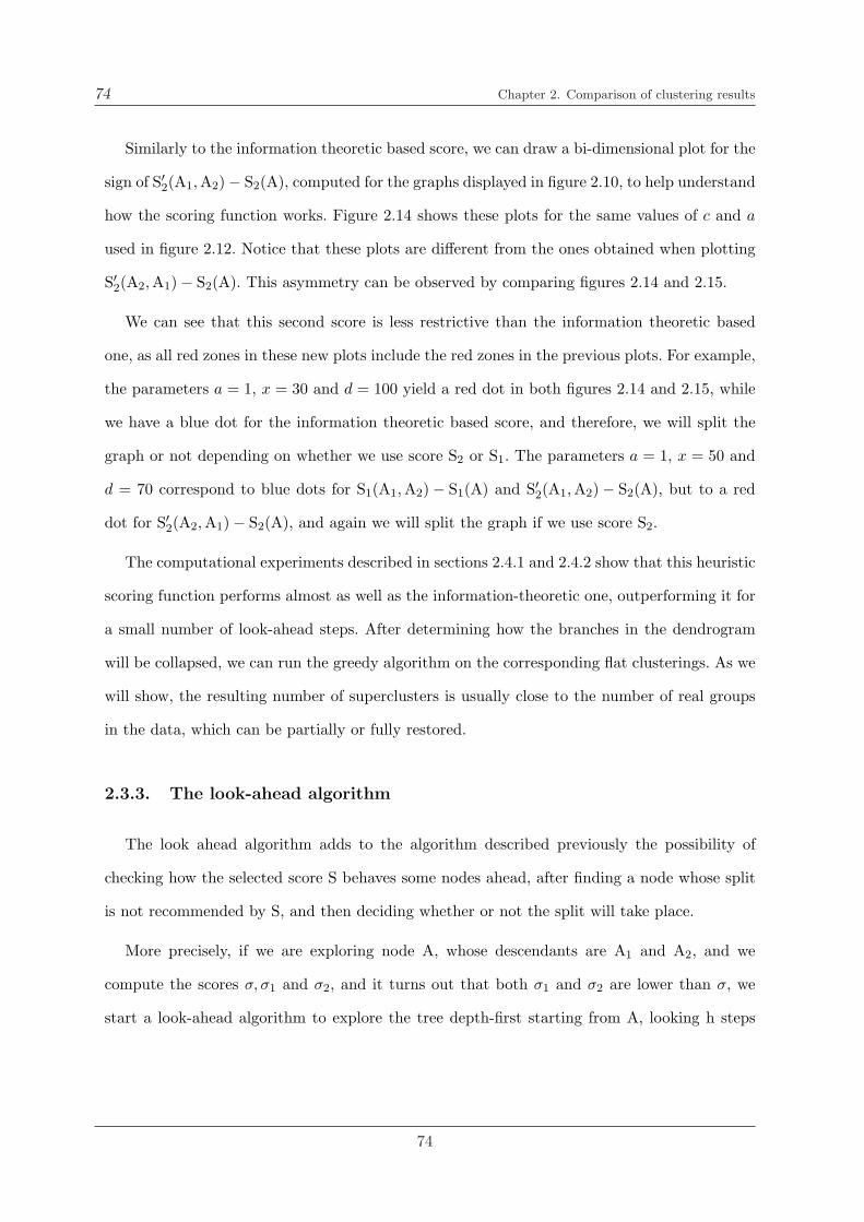
74 Chapter 2. Comparison of clustering results
Similarly to the information theoretic based score, we can draw a bi-dimensional plot for the
sign of S′2(A1, A2)− S2(A), computed for the graphs displayed in figure 2.10, to help understand
how the scoring function works. Figure 2.14 shows these plots for the same values of c and a
used in figure 2.12. Notice that these plots are different from the ones obtained when plotting
S′2(A2, A1)− S2(A). This asymmetry can be observed by comparing figures 2.14 and 2.15.
We can see that this second score is less restrictive than the information theoretic based
one, as all red zones in these new plots include the red zones in the previous plots. For example,
the parameters a = 1, x = 30 and d = 100 yield a red dot in both figures 2.14 and 2.15, while
we have a blue dot for the information theoretic based score, and therefore, we will split the
graph or not depending on whether we use score S2 or S1. The parameters a = 1, x = 50 and
d = 70 correspond to blue dots for S1(A1, A2)− S1(A) and S′2(A1, A2)− S2(A), but to a red
dot for S′2(A2, A1)− S2(A), and again we will split the graph if we use score S2.
The computational experiments described in sections 2.4.1 and 2.4.2 show that this heuristic
scoring function performs almost as well as the information-theoretic one, outperforming it for
a small number of look-ahead steps. After determining how the branches in the dendrogram
will be collapsed, we can run the greedy algorithm on the corresponding flat clusterings. As we
will show, the resulting number of superclusters is usually close to the number of real groups
in the data, which can be partially or fully restored.
2.3.3. The look-ahead algorithm
The look ahead algorithm adds to the algorithm described previously the possibility of
checking how the selected score S behaves some nodes ahead, after finding a node whose split
is not recommended by S, and then deciding whether or not the split will take place.
More precisely, if we are exploring node A, whose descendants are A1 and A2, and we
compute the scores σ, σ1 and σ2, and it turns out that both σ1 and σ2 are lower than σ, we
start a look-ahead algorithm to explore the tree depth-first starting from A, looking h steps
74

2.3 Comparison of a hierarchical and a flat clustering 75
c = 150, a = 1 c = 150, a = 10
c = 150, a = 50c = 150, a = 20
xx
xx
dd
dd
Figure 2.14: Bi-dimensional plots of the sign of S2(A1, A2)− S2(A), depending on the values of
x, d and a (= 1, 10, 20, 50) for a node A with c = 150 elements.
75

76 Chapter 2. Comparison of clustering results
c = 150, a = 1 c = 150, a = 10
c = 150, a = 50c = 150, a = 20
xx
xx
dd
dd
Figure 2.15: Bi-dimensional plots of the sign of S2(A2, A1)− S2(A), depending on the values of
x, d and a (= 1, 10, 20, 50) for a node A with c = 150 elements.
76

2.3 Comparison of a hierarchical and a flat clustering 77
ahead, where h is given by the user. If, after h steps, none of the scores has improved, we do not
split the node A, otherwise we split the tree to obtain the path to the node with the highest
score. This is illustrated in Figure 2.16: when we split the branch marked with a red dot in
graph a) we get a value of the score in graph b) that is worse than the one we had without
splitting. However, if we look ahead one step further we manage to identify two distinct clusters,
corresponding to a value of the score in graph c) that is better than that of a).
�� �� ��
Figure 2.16: Performance of the look-ahead algorithm: a decrease in the value of the score in
b) with respect to that of a) is overcome with a better value in c).
When a node A is being examined to decide whether or not we are going to split it into A1
and A2 we set a pointer or finger at A to remember where we will come back if after exploring
h steps ahead there is no improvement of σ. We will denote by σ1 and σ2 the scores generalized
to the subtree enclosed between the pointer and the two new nodes that are being checked. We
have then the following four cases:
a) any of the scores σ1 or σ2 improves the value of σ and the new nodes are the
children of A, A1 and A2; then we split the node A using the ordering giving the
higher score. This case corresponds to the splitting described in the simple version
of the algorithm. We set the pointer at the next node to be explored (either A1 or
A2, because we are exploring the tree depth-first).
b) any of the scores σ1 or σ2 improves the value of σ and the new nodes, which are at
most h+1 steps apart from A, are not the children of A; then we split the node A
77

78 Chapter 2. Comparison of clustering results
using the ordering giving the higher score, because we have managed to improve σ
within the h prefixed steps. We set the pointer at the next node to be explored.
c) none of the scores σ1 or σ2 improves the value of σ but the new nodes are at most
h steps apart from A. Then we add the new nodes to the list of nodes that have to
be checked and continue to look ahead.
d) none of the scores σ1 or σ2 improves the value of σ and the new nodes are h+1
steps apart from A. Then we go back one step and jump to the next node to be
checked. If this node is not a descendant of A, then we do not split A and continue
exploring the new node.
Notice that these four cases are not considering the possibility of finding a leaf within the h
steps. In that case, we simply jump to the next node to be explored. If this is not a descendant
of A, then we do not split A.
The pseudo-code of the look-ahead algorithm is given in the Appendix.
2.4. Results
2.4.1. Results in simulated data
Example 2.5 Model 1 with cluster size 100
For comparing a flat and a hierarchical clustering, we ran k-means with k=10, 100 times on
the same data set, constructed under Model 1, with cluster sizes randomly chosen between 1 and
100, and considering noise levels ranging between 1 and 6. Since the hierarchical clustering is
deterministic we ran it only once, selecting Euclidean distance and the average linkage method.
Usually, regardless of the scoring function that we use, the algorithm collapses the dendrogram
in such a way that after forming the superclusters there are almost no differences between the
78

2.4 Results 79
number of misclassified elements in the superclusters and in the original flat clusters.
Firstly, we used the information theoretical-based scoring function, S1, using several values
of the look-ahead parameter h. We ran k-means with k larger than the real number of groups
and computed the average number of superclusters, as well as the average number of branches
in the collapsed tree.
With no look-ahead, the number of superclusters underestimates the number of true clusters,
and the percentage of misclassified elements, even with moderate levels of noise, is high. For
example, for the case of 4 real groups, with noise level σ = 4, and running k-means with k= 10,
we get more than 20 % of misclassified elements in the clustering that results from cutting
the dendrogram, even if the number of elements closer to centres other than their own is less
than 3% (see table 2.5); for 8 real groups we get even worse results: datasets with noise level
σ = 3 have a misclassification percentage larger than 15 %, while for σ = 4 is around 35%. The
average number of branches in the tree is always smaller than the real number of groups.
However, looking just one step ahead makes the average number of superclusters come close
to the real number of groups and the percentage of misclassification decrease. For example, for
4 true groups, and σ = 4, the error rate decreases in more than a 35%, while for 8 real groups
and σ = 4, it decreases in more than a 40 % (see tables 2.5 and 2.6). The average number of
branches is always larger than the number of true clusters. For further look-ahead steps, the
error rates do not decrease significantly.
Secondly, we used the aesthetics-based score S2, using the same values of h and k as we
used for S1. With no look-ahead, the restoration of the 4 true groups is accurate: for low levels
of noise (σ < 4) the percentage of misclassified elements is less than 1 % and only for σ = 6
we get values larger than 15 % (see table 2.7). Moreover, the average number of superclusters
is correctly estimated around 4. The number of branches needed to find them ranges between
5 and 9. In the case of 8 real groups the restoration is worse; the number of real groups is
underestimated in all the cases, and for σ > 3 the percentage of misclassification is larger
79

80 Chapter 2. Comparison of clustering results
than 10%, increasing up to 46% when σ = 6. Notice that even if the error rate obtained with
k-means is much smaller than that of the hierarchical classification, there is a large increase
of the error rate on the flat side when the superclusters are formed, due to the percentage
obtained on the hierarchical side. The average number of branches in this case ranges between
6 and 9.
When we look-ahead one step (see table 2.8), the percentage of misclassified elements de-
creases, while the average number of superclusters increases. With 4 real groups, the differences
are not so remarkable as those of 8 real groups, where the decrease in the percentage of mis-
classification is up to 10. However, the number of superclusters still underestimates the number
of true groups. ¥
Example 2.6 Model 2
We also checked the performance of the method on Model 2, considering noise levels (σ)
ranging between 1 and 6, using k-means with k=5. The summary of the results for the infor-
mation theoretical-based score is given in table 2.9.
Again, not looking ahead any step with this score is not enough to obtain accurate results.
In general we obtain less than two superclusters, and an average number of branches in the
dendrogram around 2. The percentage of misclassified elements is high, reaching values higher
than 40 % for noise levels ≥ 3. However, for h=1, the average number of superclusters is slightly
greater than 3, and the average number of branches needed to obtain them oscillates between
8 and 9. The percentages of misclassification decrease respect to those of h = 0. For example,
for σ = 2, the percentage for the hierarchical clustering goes from 23.62 % to 18.25 %, and for
σ = 5, it goes from 48.07% to 41.23%. In fact, the obtained percentages are not much higher
than the percentage of elements that are closer to other centres than the ones that generated
them (see figure 2.5); thus we should not expect values smaller than these for any clustering
algorithm.
When we use the aesthetics-based score, we obtain again a better performance when we do
80

2.4 Results 81
%el
emen
tsC
lust
erin
g1
Clu
ster
ing
2
Num
ber
ofN
oise
clos
erto
othe
r%
ofm
iscl
assi
fied
elem
ents
%of
mis
clas
sifie
del
emen
tsA
vera
geA
vera
ge
orig
inal
B/W
cent
res
than
num
ber
ofnu
mbe
rof
grou
psth
eir
own
Hie
rarc
hica
ltr
eeG
roup
ing
k-m
eans
(k=
10)
Gro
upin
gsu
perc
lust
ers
bran
ches
inth
etr
ee
49.
170.
00%
3.93
%3.
93%
0.76
%2.
55%
3.80
3.91
44.
360.
00%
5.72
%5.
72%
0.69
%4.
45%
3.66
3.79
43.
250.
29%
9.45
%9.
45%
0.57
%4.
03%
3.50
3.66
42.
152.
61%
20.3
8%
21.0
1%
2.38
%11
.28
%2.
893.
22
41.
845.
26%
31.8
6%
31.9
2%
6.04
%17
.68
%2.
232.
44
41.
386.
11%
50.1
1%
50.3
8%
10.7
2%
19.7
4%
1.46
1.62
88.
950.
00%
9.28
%9.
86%
5.53
%9.
19%
6.57
5.27
84.
670.
06%
12.4
8%
13.3
5%
5.91
%9.
50%
6.33
5.32
82.
590.
89%
14.9
3%
15.7
4%
3.94
%10
.14
%6.
085.
20
82.
186.
34%
33.7
1%
34.4
8%
6.13
%24
.41
%4.
444.
73
81.
587.
17%
59.7
8%
60.3
4%
10.6
1%
25.4
1%
2.27
2.69
81.
0913
.13
%75
.49
%75
.50
%20
.46
%28
.78
%1.
201.
27
Tab
le2.
5:C
ompa
riso
nbe
twee
na
hier
arch
ical
and
ano
n-hi
erar
chic
alcl
uste
ring
,wit
hno
look
-ahe
ad,c
ompu
ting
the
info
rmat
ion
theo
reti
cal-ba
sed
scor
eS
1.
81

82 Chapter 2. Comparison of clustering results
%elem
entsC
lustering1
Clustering
2
Num
berof
Noise
closerto
other%
ofm
isclassifiedelem
ents%
ofm
isclassifiedelem
entsA
verageA
verage
originalB
/Wcentres
thannum
berof
number
of
groupstheir
own
Hierarchical
treeG
roupingk-m
eans(k=
10)G
roupingsuperclusters
branchesin
thetree
49.62
0.00%
1.12%
1.56%
0.76%
0.76%
3.995.40
43.98
0.00%
2.13%
2.27%
0.91%
0.91%
4.116.88
42.98
0.24%
1.18%
1.49%
0.77%
1.43%
4.297.97
42.15
1.38%
6.88%
7.37%
2.57%
10.94%
47.68
41.52
3.06%
16.40%
18.64%
4.94%
14.02%
3.7512.15
41.27
6.58%
29.93%
30.40%
10.04%
6.31%
2.76.65
89.14
0.00%
4.88%
6.31%
6.31%
3.96%
6.958.60
84.29
0.04%
2.77%
3.98%
3.96%
3.65%
7.28.40
83.17
1.05%
4.62%
5.92%
3.65%
5.78%
7.0510.77
82.04
4.39%
12.15%
14.69%
5.78%
1.42%
6.3614.05
81.93
3.81%
40.57%
42.72%
11.42%
11.42%
4.0912.42
81.18
13.49%
54.69%
55.69%
17.38%
17.38%
2.612.20
Table
2.6:C
omparison
between
ahierarchical
anda
non-hierarchicalclustering,
usingthe
look-aheadalgorithm
,searching
one
stepahead
andcom
putingthe
information
theoretical-basedscore
S1 .
82

2.4 Results 83
%el
emen
tsC
lust
erin
g1
Clu
ster
ing
2
Num
ber
ofN
oise
clos
erto
othe
r%
ofm
iscl
assi
fied
elem
ents
%of
mis
clas
sifie
del
emen
tsA
vera
geA
vera
ge
orig
inal
B/W
cent
res
than
num
ber
ofnu
mbe
rof
grou
psth
eir
own
Hie
rarc
hica
ltr
eeG
roup
ing
k-m
eans
(k=
10)
Gro
upin
gsu
perc
lust
ers
bran
ches
inth
etr
ee
49.
360.
00%
0.24
%0.
25%
0.21
%0.
25%
4.43
8.88
44.
210.
00%
0.21
%0.
22%
0.19
%0.
19%
4.38
8.55
43.
040.
15%
0.77
%0.
95%
0.69
%0.
85%
4.34
8.46
42.
231.
64%
3.46
%5.
22%
2.28
%4.
78%
4.31
7.78
41.
683.
21%
9.74
%13
.73
%5.
65%
13.4
7%
3.67
6.59
41.
156.
79%
17.1
9%
20.7
1%
10.7
6%
20.1
7%
3.24
5.41
89.
250.
00%
7.15
%7.
91%
5.77
%7.
91%
6.75
9.12
84.
760.
02%
4.31
%4.
84%
4.01
%4.
82%
7.10
9.21
83.
501.
15%
4.14
%5.
71%
3.33
%5.
29%
7.14
9.06
82.
164.
27%
12.1
4%
13.7
3%
5.54
%12
.41
%6.
427.
71
81.
823.
96%
29.3
1%
31.3
8%
11.7
7%
29.7
5%
4.89
6.14
81.
0712
.28
%42
.51
%46
.04
%19
.14
%44
.98
%3.
566.
08
Tab
le2.
7:C
ompa
riso
nbe
twee
na
hier
arch
ical
and
ano
n-hi
erar
chic
alcl
uste
ring
,w
ith
nolo
ok-a
head
,co
mpu
ting
the
aest
heti
cs-
base
dsc
ore
S2.
83

84 Chapter 2. Comparison of clustering results
%elem
entsC
lustering1
Clustering
2
Num
berof
Noise
closerto
other%
ofm
isclassifiedelem
ents%
ofm
isclassifiedelem
entsA
verageA
verage
originalB
/Wcentres
thannum
berof
number
of
groupstheir
own
Hierarchical
treeG
roupingk-m
eans(k=
10)G
roupingsuperclusters
branchesin
thetree
49.84
0.00%
0.15%
0.25%
0.25%
0.25%
4.8610.79
44.19
0.00%
0.32%
0.64%
0.31%
0.64%
4.8811.54
43.17
0.04%
0.70%
2.14%
0.68%
2.08%
4.8711.56
42.23
1.74%
2.87%
6.31%
2.46%
6.01%
4.6111.20
41.81
5.73%
7.92%
13.87%
6.26%
13.34%
4.069.21
41.19
6.46%
12.05%
18.91%
10.55%
18.51%
3.628.39
89.55
0.00%
3.04%
5.11%
5.11%
5.11%
7.1311.10
84.39
0.00%
3.00%
4.40%
4.37%
4.38%
7.4510.67
83.28
0.65%
3.78%
5.82%
3.40%
5.45%
7.2410.68
82.19
6.83%
6.98%
9.49%
5.84%
8.28%
6.839.66
81.88
3.95%
19.11%
23.50%
11.34%
21.66%
5.809.06
81.25
13.25%
32.48%
39.86%
19.74%
38.08%
4.328.73
Table
2.8:C
omparison
between
ahierarchical
anda
non-hierarchicalclustering,
usingthe
look-aheadalgorithm
,searching
one
stepahead
andcom
putingthe
aesthetics-basedscore
S2 .
84

2.4 Results 85
Clustering 1 Clustering 2
% misclassified elements % misclassified elements Average Average
h Hierarchical k-means number of number of
tree Grouping (k=5) Grouping superclusters branches
0 5.03% 5.13% 0.74% 1.98% 3.02 3.43
0 23.29% 23.62 % 13.72% 20.50 % 2.49 2.85
0 39.66% 40.32 % 25.30% 31.67 % 1.79 2.03
0 45.43% 45.88 % 31.78% 37.87 % 1.55 1.85
0 47.89% 48.07 % 36.85% 40.75 % 1.36 1.48
0 48.44% 48.62 % 39.40% 42.59 % 1.39 1.59
1 0.61% 1.00% 0.74% 0.98% 3.81 6.39
1 15.53% 18.25 % 13.18% 18.16 % 3.76 8.76
1 29.30% 32.20 % 25.48% 28.17 % 3.56 8.98
1 33.99% 37.18 % 31.87% 34.25 % 3.57 9.42
1 37.78% 41.23 % 35.96% 37.82 % 3.45 8.73
1 40.90% 44.29 % 39.62% 41.44 % 3.18 8.97
Table 2.9: Comparison between a hierarchical and a non-hierarchical (k=5) clustering, using
the look-ahead algorithm, with h= 0 and 1, and the information theoretical-based score S1.
85

86 Chapter 2. Comparison of clustering results
Clustering 1 Clustering 2
% misclassified elements % misclassified elements Average Average
h Hierarchical k-means number of number of
tree Grouping (k=5) Grouping superclusters branches
0 1.07% 1.21% 1.06% 1.14% 3.69 4.57
0 16.61% 17.21 % 13.64% 17.01 % 3.63 4.52
0 28.29% 29.30 % 24.97% 29.02 % 3.38 4.49
0 33.58% 35.31 % 32.28% 35.15 % 3.68 5.28
0 37.70% 39.40 % 35.55% 39.22 % 3.47 5.11
0 41.54% 42.83 % 40.59% 42.97 % 3.52 5.16
1 1.54% 1.80% 1.68% 1.68% 4.27 6.52
1 13.41% 15.13 % 13.82% 15.32 % 4.12 6.68
1 25.88% 28.45 % 25.19% 28.46 % 3.98 6.85
1 32.28% 34.76 % 32.05% 34.61 % 3.90 6.82
1 36.32% 38.20 % 36.01% 38.09 % 3.91 6.89
1 39.19% 41.66 % 39.15% 41.34 % 3.85 7.14
Table 2.10: Comparison between a hierarchical and a non-hierarchical (k=5) clustering, using
the look-ahead algorithm, with h= 0 and 1, and the aesthetics-based score S2.
86

2.4 Results 87
not look ahead any further, due to the fact that S2 is less restrictive than S1 (see the summary
in table 2.10). The average number of superclusters is close to 3, and the number of branches
needed to identify them is between 4 and 5. The percentages of misclassification are very similar
to those obtained for S1 and h = 1. On the other hand, when h=1, the number of superclusters
is around 4 and the percentage of misclassification does not decrease significantly.
In brief, it appears that the visualization aesthetics-based scoring function outperforms the
MDL principle for a small number of look-ahead steps. Therefore it can be used to improve
the execution time (in our implementation it takes seconds to compare clusters of thousands
of genes without look-ahead, and minutes with look-ahead).
2.4.2. Results in real data
We also tested the algorithm on real data. As an example, Figure 2.17 shows the compari-
son of a hierarchical clustering (where we selected correlation-based distance and the average
linkage method) to a k-means clustering (with correlation-based distance and k=5 clusters)
of the Schizosaccharomyces pombe stress response dataset (Chen et al., 2003), (ArrayExpress
accession number E-MEXP-29).
This set, available at http://www.sanger.ac.uk/PostGenomics/S pombe/projects/stress/,
characterizes the changes in expression profiles of all known and predicted genes of the fis-
sion yeast S. pombe in response to five stress conditions (oxidative stress caused by hydrogen
peroxide, heavy metal stress caused by cadmium, heat shock caused by temperature increase
to 39oC, osmotic stress caused by sorbitol, and DNA damage caused by the alkylating agent
methylmethane sulfonate), measured using DNA microarrays in three strains (wild-type and
two mutants: sty1∆ and atf1∆). The data set was filtered so that we retain the 140 most
varying ones (≥ 0.9 standard deviations in 60 % of the hybridizations). Then we applied the
algorithm; we used no look-ahead, and scoring function S2. The highly-responding (yellow) clus-
ter is highly enriched with the so-called CESR (Core Environmental Stress Response) genes.
87

88 Chapter 2. Comparison of clustering results
These are genes that are up-regulated in at least four of the five conditions or down-regulated
in at least three of the five conditions. The up-regulated cluster contains 12 of such genes out of
64. Near the middle of the hierarchical tree, the cluster of genes of high negative response (blue)
are mostly mitochondrial ones. The down-regulated CESR genes are also enriched (25/62).
Figure 2.17: A comparison of the hierarchical clustering of (correlation-based distance, average
linkage) ∼ 140 most varying genes ( ≥ 0.9 standard deviations in 60 % of the hybridizations) in
the S. pombe stress response dataset to a k-means clustering of the same dataset (correlation-
based distance, k=5).
This example shows that, when applying the comparison algorithm to real gene expression
data, we can obtain biologically meaningful results, which helps expert biologists to explore
their data.
88

2.5 Implementation in Expression Profiler 89
2.5. Implementation in Expression Profiler
The algorithms described in previous sections are available through the online gene expres-
sion data analysis tool Expression Profiler (EP) (Kapushesky et al., 2004) at the European
Bioinformatics Institute (EBI) (http://www.ebi.ac.uk/expressionprofiler). A user can upload
a gene expression matrix together with associated annotations to the EP platform, where a
number of analytical components are available, including data transformation, sub-selection,
statistical tests and clustering, both hierarchical and k-means. The Clustering Comparison
component, under the “Clustering” menu allows the user to run the algorithm and view the vi-
sualization of the output. The user is presented with the analysis history of the current dataset
and can select a pair of previously performed clusterings to be compared. Alternatively, the
user can select a dataset to be analysed and set up two sets of clustering parameters. In this
case the two clusterings will be executed and then their results will be compared and the vi-
sual display will be produced. For running hierarchical clusterings the user needs to specify a
distance measure (e.g., Euclidean or Pearson correlation, etc.) and type of linkage (complete,
average, etc.). Similarly, the distance measure should be specified for flat clusterings, as well
as the number k for k-means.
Adjustable clustering comparison algorithm parameters are also presented. The user can
specify the number of steps to use in the look-ahead tree search and the type of scoring function
to use (information-theoretic or aesthetics-based).
The underlying clustering comparison algorithm is implemented in R. The source code is
available as part of the open-source distribution of Expression Profiler. The EP data analysis
tool also provides a visualization of the comparison (see Figure 2.17), displaying side-by-side the
tree, with optimal cut-off points marked in red, the expression heatmap, gene annotations, the
set of k clusters resulting from the flat clustering, and the clustering comparison correspondence.
The latter is depicted as lines of varying thickness, mapping sub-branches of the tree to flat
clustering superclusters. Line thickness is proportional to the number of elements common to
89

90 Chapter 2. Comparison of clustering results
both sets; by placing the mouse cursor over a line, a Venn diagram is displayed with the exact
numbers – how many elements are in the cluster generated by cutting the respective branch,
how many in the corresponding flat cluster and how many of these two overlap.
In summary, from the results shown in this chapter we can conclude that the novel method
that we have developed allows the user to explore relationships between different clustering
results, including hierarchical clusterings without any a priori given cut-offs. Although the
biological relevance of the comparison results depends on the clusters that are compared, in
some cases it is possible to improve the original clustering.
90

Capıtulo 3
Refinamientos robustos de k-medias
mediante profundidad
Resumen
Muchas tecnicas iterativas son sensibles a las condiciones iniciales, por lo que pueden quedar
atrapadas en optimos locales. Este capıtulo explora dos metodos simples y computacional-
mente rapidos que permiten el refinamiento de los puntos iniciales de k-medias para agru-
par las observaciones de un conjunto dado. Se basan, respectivamente, en alternar k-medias
con la busqueda del dato mas profundo (mas representativo) de cada cluster, y en combinar
bootstrap con la busqueda de los datos mas profundos de cada cluster en el espacio de los
centros bootstrap. Ademas, combinada con la construccion de regiones de Voronoi generaliza-
das a lugares geometricos convexos, esta segunda alternativa puede proporcionar un clustering
“no rıgido” que asigna a cada elemento del conjunto de datos un ındice de pertenecia a cada
cluster. Esto es una alternativa util en ciertos campos, como en expresion genica, donde los
datos analizados pueden pertenecer simultaneamente a varios clusters. Estos metodos se han
probado en observaciones simuladas, incluyendo modelos contaminados, y en datos reales, y
han demostrado ser eficientes y mas rapidos que el metodo DDclust, propuesto en Jornsten
(2004).
91

92 Capıtulo 3. Refinamientos robustos de k-medias mediante profundidad
3.1. Introduccion
Es bien sabido que k-medias y otras tecnicas iterativas (e.g. el algoritmo EM) son especial-
mente sensibles a las condiciones iniciales, i.e., a menudo el proceso puede obtener solo uno
de los optimos locales del problema considerado, lo cual puede conducir a conclusiones muy
distintas en el analisis de un mismo conjunto de observaciones. Puesto que se ha demostra-
do que el problema de obtener un estado inicial globalmente optimo es de complejidad NP
(Garey y Johnson, 1979; Garey et al., 1982), resulta mas practico y valioso estudiar metodos
de inicializacion dirigidos a encontrar una solucion suboptima del problema de clustering.
Existen varios metodos de inicializacion de algoritmos iterativos, que pueden ser divididos
principalmente en tres grandes categorıas (He et al., 2004):
metodos de muestreo aleatorio, que son, probablemente, los mas usados en la li-
teratura y siguen una forma “ingenua” de determinar los clusters iniciales, o bien
seleccionando aleatoriamente observaciones muestrales, o bien eligiendo parametros
aleatorios generados de forma no heurıstica a partir de los datos. Como ejemplo,
veanse Forgy (1965) o MacQueen (1967).
metodos de optimizacion de distancias, cuyo objetivo es optimizar las distancias
entre los clusters iniciales para obtener en el resultado una separacion inter-cluster
satisfactoria Veanse como ejemplo (Tou y Gonzalez, 1974; Katsavounidis et al.,
1994).
metodos de estimacion de la densidad, que se basan en la suposicion de que los
datos siguen una distribucion de mixturas gaussianas e intentan identificar en ellos
areas densas que ayuden a crear clusters compactos (Kaufman y Rousseeuw, 1990;
Al-Daoud y Roberts, 1994).
92
3.1 Introduccion 93
Existe ademas otra categorıa de estudios en los cuales estamos interesados y que tratan
el refinamiento del estado inicial de los metodos de clustering. Estos estudios incluyen un
refinamiento propuesto por Bradley y Fayyad (1998) que elige inicialmente J submuestras ale-
atorias de pequeno tamano de los datos, Si, i = 1, ..., J . Entonces, las submuestras se agrupan
mediante k-medias, imponiendo la condicion de que en los clusters que terminen vacıos se
reasignaran sus correspondientes centros iniciales, y la submuestra sera reagrupada. Los con-
juntos CMi, i = 1, ..., J , son los clusterings que resultan de las submuestras, y conforman el
conjunto CM . Finalmente, CM es agrupado para cada i, usando k-medias inicializada con
CMi, lo cual proporciona la solucion FMi. Los puntos iniciales (semillas) refinados se escogen
como la solucion FMi que tiene menor distorsion sobre el conjunto CM .
Tambien existen algoritmos geneticos disenados para refinar los puntos iniciales de k-medias,
pero tienen una gran carga computacional; por ejemplo, vease el metodo descrito por Laszlo y
Mukherjee (2006) para datos de baja dimension.
En una lınea de investigacion diferente, Jornsten (2004) propuso un metodo de clustering
robusto, el algoritmo DDclust , basado en el concepto de profundidad, para resolver el problema
de minimizar la suma de las distancias L1 de las observaciones al representante mas cercano
de los clusters.
Una profundidad es una medida de lo central o exterior que es una observacion dada con
respecto a una nube de puntos o a una distribucion. Las funciones de profundidad introducen un
orden desde el centro hacia fuera en los datos multidimensionales. En Estadıstica, la motivacion
y la necesidad de generalizar la mediana y el rango es muy natural, puesto que la media no
es una medida robusta de posicion central. La profundidad considerada en Jornsten (2004) es
la profundidad L1 de Vardi y Zhang (2000), cuya interpretacion estadıstica es la probabilidad
que se necesita en un punto z para que dicho punto sea la mediana L1 multivariante del
93

94 Capıtulo 3. Refinamientos robustos de k-medias mediante profundidad
cluster – i.e., un representante robusto del cluster. Esta es la primera propuesta de un metodo
de clustering en el que se usa el concepto de profundidad, y combina la busqueda de estas
medianas multivariantes con la asignacion a los vecinos mas proximos, ademas de incluir una
tecnica de “recocido simulado” (simulated annealing), para evitar quedarse atrapado en un
mınimo local.
En este capıtulo nos proponemos obtener un procedimiento de refinamiento del estado ini-
cial de k-medias, combinando ideas de Bradley y Fayyad (1998) y Jornsten (2004), utilizando
una generalizacion finito-dimensional de la mediana univariante diferente de la empleada en
Jornsten (2004). La profundidad que utilizamos es la denominada profundidad por bandas gene-
ralizada, descrita en Lopez-Pintado y Romo (2006), aunque cualquier definicion de profundidad
de datos multidimensionales podrıa utilizarse en nuestro metodo.
Una primera propuesta para refinar k-medias es la siguiente. Supongamos que hemos agru-
pado el conjunto X en k grupos mediante k-medias, con los centros iniciales elegidos aleatoria-
mente. Sea cual sea la profundidad elegida, hallamos el dato mas profundo (mas central) Di en
cada uno de los k clusters obtenidos, y usamos estos nuevos puntos como centros iniciales en
el algoritmo de k-medias. Si esto conlleva una reduccion en la funcion objetivo, continuamos
iterando con los nuevos puntos mas profundos que obtengamos usados como centros iniciales; en
otro caso, mantenemos el resultado de k-medias que proporciona el valor mınimo en la funcion
objetivo. De esta forma, no podemos obtener resultados peores que los derivados de k-medias
en terminos de la funcion objetivo. Sin embargo, hay que observar que los conglomerados reales
con que nos encontramos en la practica no siempre minimizan la funcion objetivo y, ası, valores
mas pequenos de la distorsion se corresponden con un numero superior de observaciones mal
asignadas, y viceversa. Los resultados obtenidos en este enfoque muestran que este procedimien-
to de refinamiento funciona bien para una gran variedad de conjuntos de datos, pero puede
94

3.1 Introduccion 95
ocurrir que k-medias encuentre un (mal) optimo local del cual nuestro metodo no es capaz
de “escapar”. Por ello, proponemos una alternativa basada en extraer muestras bootstrap del
conjunto de observaciones para obtener una coleccion de centros C, que es agrupada mediante
k-medias; finalmente, en cada cluster (de centros) se halla el dato mas profundo, para usarlos
como puntos iniciales de k-medias. Este procedimiento proporciona un metodo muy eficiente y
robusto, que supera a k-medias en todos los casos y se comporta de manera semejante a la de
DDclust, pero es mucho mas rapido.
Este capıtulo esta organizado como sigue. La seccion 3.2 proporciona una manera eficiente
de calcular la profundidad por bandas generalizada, y describe dos metodos nuevos, GBDRk
(k-medias refinada por la profundidad por bandas generalizada) en la subseccion 3.2.2, y BRk
(k-medias refinada por bootstrap) en la subseccion 3.2.3, que permiten el refinamiento de los
puntos iniciales de k-medias. Estos dos algoritmos se basan, respectivamente, en alternar k-
medias con la busqueda del dato mas profundo en cada cluster y en combinar resultados de
bootstrap sobre k-medias con la busqueda de los puntos mas profundos de cada cluster en
el espacio de los centros de los clusters. El comportamiento de ambos metodos se compara
con el de otros metodos utilizados en la literatura, usando tanto datos simulados como reales.
Finalmente, en la seccion 3.4 describimos como emplear el metodo BRk para proporcionar un
clustering no rıgido de las observaciones, lo que es util en campos como el analisis de datos de
expresion genica, en el que los genes pueden pertenecer a mas de un cluster.
95

96 Capıtulo 3. Refinamientos robustos de k-medias mediante profundidad
3.2. Metodos
3.2.1. Un calculo eficiente de la profundidad por bandas generalizada
En Estadıstica no parametrica existen diversas medidas de profundidad como generaliza-
ciones del rango con el objetivo de complementar el analisis multivariante clasico, primero por
Tukey (1975), seguido posteriormente por Oja (1983), Liu (1990), y Donoho y Gasko (1992), en-
tre otros. Sin embargo, una de las mayores desventajas en todas las definiciones de profundidad
de datos es el coste computacional asociado, lo que restringe su uso a conjuntos de observaciones
de baja dimension. Nuestro procedimiento, que sera descrito en la seccion siguiente, permite el
uso de cualquier definicion de profundidad, aunque nosotros hemos empleado la profundidad
por bandas generalizadas descrita en Lopez-Pintado y Romo (2006), que resulta apropiada
para datos de alta dimension, para reducir el tiempo de computacion. Sea Y = {y1, . . . , yn} un
conjunto de n puntos d-dimensionales, y denotemos por yi,k, i = 1, ..., n, la k-esima componente
del elemento yi. La version finito-dimensional de la profundidad por bandas generalizada GBD
de un punto y se define como la proporcion media de las componentes de y que se encuentran
entre las correspondientes componentes de todos los posibles pares de elementos de Y . Mas
formalmente:
GBD(y) =1(n
2
)∑
1≤i1<i2≤n
1d
d∑
k=1
I{min(yi1,k,yi2,k)≤yk≤max(yi1,k,yi2,k)} (3.2.1)
Observese que la profundidad por bandas generalizada se puede calcular de forma muy
eficiente rescribiendo la expresion 3.2.1 como se describe en la siguiente proposicion.
Proposicion 3.1 Dados un conjunto de observaciones Y = {y1, ..., yn}, y un punto yi ∈ Y con-
96

3.2 Metodos 97
sideremos las matrices Y =
y1,1 . . . y1,d
......
yn,1 . . . yn,d
and Y =
y(1),1 . . . y(1),d
......
y(n),1 . . . y(n),d
, donde
cada columna en Y ha sido organizada en orden creciente. Sea lk el menor ındice en la k-esima
columna de Y que verifica yi,k = y(lk),k, y sea ηk la multiplicidad del valor yk en la misma.
Entonces, la profundidad por bandas generalizada del punto yi esta dada por
1d× (
n2
)d∑
k=1
((n− lk + 1)(lk − 1 + ηk)− η2
k +(
ηk
2
)). (3.2.2)
Demostracion: Notese que
GBD(yi) =1(n
2
)∑
1≤i1<i2≤n
1d
d∑
k=1
I{min(yi1,k,yi2,k)≤ yi,k≤max(yi1,k,yi2,k)} =
=1(n
2
) 1d
d∑
k=1
∑
1≤i1<i2≤n
I{min(yi1,k,yi2,k)≤ yi,k}I{max(yi1,k,yi2,k)≥ yi,k} =
=1(n
2
) 1d
d∑
k=1
∑
1≤i1<i2≤n
(I{min(yi1,k,yi2,k)< yi,k} + I{min(yi1,k,yi2,k)= yi,k}
)×
×(I{max(yi1,k,yi2,k)> yi,k} + I{max(yi1,k,yi2,k)= yi,k}
)=
=1
d× (n2
)d∑
k=1
[(lk − 1) · (n− (lk + ηk − 1)) + (lk − 1) · ηk +
+ ηk · (n− (lk + ηk − 1)) +(
ηk
2
)] =
=1
d× (n2
)d∑
k=1
((n− lk + 1)(lk − 1 + ηk)− η2
k +(
ηk
2
)).
¥
Este calculo reduce significativamente el coste computacional. Por ejemplo, implementar la
97

98 Capıtulo 3. Refinamientos robustos de k-medias mediante profundidad
profundidad en R implica una reduccion con respecto al calculo de la correspondiente propor-
cion para todos los pares, que es O(d.n2), a O(n4/3) para reordenar la matriz Y usando una
variante de (Sedgewick, 1986) mas O(d) para calcular el valor 3.2.2.
3.2.2. Alternancia de k-medias con la busqueda de datos mas profundos
Consideremos un conjunto X en Rd, cuyos elementos se quieren agrupar en k grupos. De-
notemos por C1, . . . Ck los centros de estos grupos y por ∆ la funcion objetivo o distorsion, dada
por la suma de las distancias al cuadrado entre cada punto x ∈ X y el centro mas cercano
Ci(x). El metodo de k-medias refinado por la profundidad por bandas generalizada (GBDRk)
se describe formalmente mas abajo mediante un pseudo-codigo. Los valores de entrada para
el metodo son el conjunto de observaciones X, el numero de conglomerados k que se desea
obtener y el numero maximo de iteraciones, max.iter.
Cuadro 3.2.2.1. Algoritmo iterativo de seleccion de centros iniciales basado en el concepto
de profundidad de datos.
no.iterations ← 0
WHILE (no.iterations < max.iter ) DO:
1. no.iterations ← no.iterations + 1
2. Usar k-medias en X iniciado con k puntos elegidos aleatoriamente para obtener k
clusters, I11 , ..., I1
k , con centros respectivos C11 , . . . C1
k .
3. Calcular la suma de distancias al cuadrado de cada punto a su centro mas proximo
∆1.
98

3.2 Metodos 99
4. Encontrar el punto mas profundo de cada cluster: D11 ∈ I1
1 , . . . ,D1k ∈ I1
k .
5. Usar k-medias, con puntos iniciales D11, . . .D1
k, para obtener k nuevos clusters
I21 , ..., I2
k con centros C21 , . . . C2
k .
6. Calcular la suma de las distancias al cuadrado ∆2 para el nuevo clustering.
7. IF ∆2 < ∆1
THEN
I1j ← I2
j , j = 1, ..., k; ∆1 ← ∆2
ir al paso 3
OTHERWISE
dar como resultado el clustering I11 , ..., I1
k y parar
Este algoritmo de refinamiento da como resultado un clustering que proporciona un valor de
la funcion objetivo que es al menos tan buena como la que da k-medias, porque si la utilizacion
de los datos mas profundos como centros iniciales no mejora esta funcion, entonces conservamos
el resultado original de k-medias.
En general, los resultados obtenidos en datos simulados y reales con este procedimiento
demuestran que se comporta mejor que k-medias, pero para algunos conjuntos de datos, el
metodo propuesto no es capaz de mejorar algunos malos resultados, en los que k-medias se
queda “atascada”. Una alternativa podrıa ser utilizar una tecnica de recocido simulado (si-
mulated annealing) para escapar de los optimos locales, como en el caso de DDclust; esto
sera objeto de investigacion futura. En su lugar, en la seccion siguiente describiremos un en-
99

100 Capıtulo 3. Refinamientos robustos de k-medias mediante profundidad
foque diferente basado en hacer bootstrap sobre el conjunto de observaciones X, combinado
con la busqueda del dato mas profundo de cada cluster, que resulta ser muy robusto y mejora
a k-medias, a la vez que es comparable con DDclust, con la ventaja de ser mucho mas rapido.
3.2.3. Combinacion de bootstrap con la busqueda de datos mas profundos
Como se menciono en la seccion 3.2.2, estamos interesados en encontrar un metodo alterna-
tivo que refine las semillas a un nuevo conjunto de puntos que esten proximos a los maximos
(modas) de la funcion de densidad de los datos. De forma similar a Bradley y Fayyad (1998),
proponemos una heurıstica basada en remuestrear (en particular, usando bootstrap) los datos
B veces, y utilizar k-medias estandar con k clusters en cada muestra bootstrap, b = 1, . . . , B,
para obtener un conjunto C de b · k centros estimados; finalmente, buscamos k nuevos clusters
en C, y usamos el dato mas profundo de cada cluster como semillas iniciales.
La heurıstica se basa en el concepto de bagging (Breiman, 1996) usado en aprendizaje super-
visado, que combina las clasificaciones predichas a partir de diferentes datos de entrenamiento
mediante algun esquema de votacion simple; la clasificacion final obtenida para cada dato es
la correspondiente a la mas frecuente entre las predichas.
Existe trabajo previo de bagging aplicado a clustering. Leisch (1999) diseno un “bagged
clustering” que combina metodos de particion y metodos jerarquicos. Su algoritmo obtiene una
coleccion de conjuntos de entrenamiento usando bootstrap, a continuacion utiliza cualquier
clustering no jerarquico en cada uno de estos conjuntos, y finalmente combina las particiones
resultantes usando clustering jerarquico. Dudoit y Fridlyand (2003) propusieron otros dos meto-
dos que extienden el concepto de bagging al clustering. Uno de estos se basa en un criterio de
votacion y el otro en la creacion de una nueva matriz de disimilaridades. En nuestro procedi-
100
3.2 Metodos 101
miento de aprendizaje no supervisado, el papel de la clasificacion mas votada es desempenado
por los clusters existentes en C, y usamos como representantes iniciales de los clusters en el
espacio original el dato mas profundo de tales clusters.
Como en Leisch (1999), nuestro metodo, en primer lugar, transforma el problema de clus-
tering en el espacio de los datos originales en un nuevo problema en el espacio de los centros
producidos por k-medias. Supongamos que el conjunto de observaciones X se genera por una
distribucion F desconocida, con densidad f . Asumamos que f es multimodal y que cada moda
corresponde a un cluster. Si los centros producidos por k-medias se concentran en las modas
de f , entonces los nuevos clusters son mas pequenos en el sentido euclidiano –y de hecho, para
cualquier distancia– que los originales, con mayor probabilidad. Esto puede verse en el Teore-
ma 2 de Leisch (1999). La diferencia con el enfoque de Leisch es que nosotros fijamos a priori
el numero de clusters que estamos buscando (recordemos que nuestro objetivo es refinar los
puntos iniciales de k-medias) y que la busqueda del dato mas profundo de cada cluster en un
contexto multivariante es mas robusto, lo cual atenua la influencia de muestras bootstrap poco
representativas.
Nuestro algoritmo esta descrito mediante pseudo-codigo en el cuadro 3.2.3.1. De nuevo,
denotamos por X un conjunto de observaciones en Rd, cuyos elementos van a ser agrupados
en k clusters. Los datos de entrada son el conjunto X, el numero de clusters k que vamos a
obtener y el numero de replicaciones bootstrap B.
101

102 Capıtulo 3. Refinamientos robustos de k-medias mediante profundidad
1. FOR (b in 1 : B ) DO:
- Obtener la muestra bootstrap Xb del conjunto X.
- Usar k-medias con k puntos iniciales, elegidos aleatoriamente, sobre el conjunto Xb
para obtener k clusters, Ib1, ..., I
bk, con centros respectivos Cb
1, . . . Cbk. Si alguno de los
clusters queda vacıo, volver a usar k-medias con diferentes puntos iniciales.
2. Usar k-medias en C = {Cbi , i = 1, ..., k, b = 1, ..., B} para obtener k clusters,
I∗1 , ..., I∗k .
3. Encontrar el punto mas profundo de cada cluster: D1 ∈ I∗1 , . . . ,Dk ∈ I∗k .
4. Usar k-medias con puntos iniciales D11, . . .D1
k.
5. Dar como resultado el clustering I1, ..., Ik.
Box 3.2.3.1. Algoritmo de seleccion de los centros iniciales basado en la combinacion de
bootstrap con el concepto de profundidad de datos.
Observemos que una pequena variacion en el metodo permite transformar el procedimiento
de refinamiento en un algoritmo de clustering en sı mismo: en lugar de usar el dato mas profundo
de cada cluster en el espacio de los centros D1 ∈ I∗1 , . . . ,Dk ∈ I∗k como puntos iniciales de k-
medias, estos pueden ser utilizados como centroides (finales) y podemos asignar cada elemento
de X al centroide mas proximo, definiendo ası el clustering. Esto es equivalente a usar solo la
primera iteracion de k-medias en el Paso 4 del metodo BRk, y en general se deberıan obtener
resultados muy similares.
Se puede demostrar que el metodo BRk, bajo ciertas condiciones de simetrıa y de regu-
laridad, es consistente, simplemente combinando los resultados correspondientes de k-medias
102

3.2 Metodos 103
(Pollard, 1982), de bootstrap de M-estimadores (Arcones y Gine, 1992) y de datos mas pro-
fundos (Lopez-Pintado y Romo, 2006).
Teorema 3.1 Sea P una distribucion simetrica en Rd y supongamos
i) el vector µ = (µ1, . . . , µk) que minimiza la suma de cuadrados intra-clusters pobla-
cional W (·) es unico excepto por permutacion de sus coordenadas;
ii) P‖x‖2 < ∞;
iii) P tiene una densidad continua f .
Entonces, el vector de los puntos mas profundos D calculados en el metodo BRk es consistente
para estimar el vector µ.
Demostracion: En primer lugar, siguiendo los resultados de Arcones y Gine (1992) para
la aproximacion bootstrap de M-estimadores, los centros boostrap {Cb1, . . . Cb
k}, b = 1, . . . , B
calculados en el Paso 1 son estimadores consistentes de las localizaciones de los centros, i.e.,
excepto por permutacion de coordenadas se tiene:
Cbi → µi, b = 1, . . . , B, i = 1, . . . , k.
A continuacion, observemos que en el espacio de los centros (bootstrap), las condiciones i)
y ii) se verifican, por lo que, usando el teorema central del lımite de Pollard (1982), aplicar k-
medias en este espacio implica que las correspondientes localizaciones de los centros convergen
en probabilidad al vector µ.
Finalmente, como la profundidad por bandas generalizada es consistente, los correspondien-
tes datos mas profundos D11, . . .D1
k convergen a los datos mas profundos del espacio inicial, que
103

104 Capıtulo 3. Refinamientos robustos de k-medias mediante profundidad
coinciden con µ si la distribucion es simetrica. ¥
En general, para datos generados, BRk tiene un comportamiento muy robusto, similar e in-
cluso mejor en ocasiones que los de DDclust, siendo ambos los mejores de los metodos analiza-
dos. BRk consigue disminuir tanto la distorsion como el porcentaje de elementos mal asignados
por k-medias, y proporciona sus resultados en mucho menos tiempo que DDclust.
3.3. Resultados
3.3.1. Resultados en datos simulados
Los experimentos de simulacion fueron realizados como sigue. Para cada modelo particular
creamos cincuenta conjuntos de datos y usamos el algoritmo de k-medias estandar, el algoritmo
PAM, el algoritmo CLARA, DDclust, k-medias refinada por la profundidad por bandas gene-
ralizada (GBDRk) y k-medias refinada por bootstrap (BRk). En todos los algoritmos usamos
el mismo numero de clusters, que correspondıa con el numero real de grupos simulados. Para
evaluar el comportamiento de estos metodos en terminos de la distorsion, calculamos su valor
obtenido para cada conjunto. Observemos, no obstante, que PAM, CLARA y DDclust estan
disenados para minimizar la suma de distancias y no la distorsion. Para evaluar el compor-
tamiento de estos metodos en terminos del error de asignacion, calculamos las tasas de error
y las representamos en diagramas de caja y en tablas que contienen los cuartiles, ası como los
valores mınimo y maximo.
Para evaluar el comportamiento de los metodos en presencia de datos atıpicos, tambien
empleamos diferentes modelos contaminados. Un modelo contaminado se construye como sigue:
la mayor parte de los puntos de un cluster se obtienen de una distribucion “progenitora”
Pp, mientras que los restantes puntos, en una proporcion de ε, proceden de otra distribucion
104

3.3 Resultados 105
denotada por Pc. Empleamos los siguientes modelos:
a) Contaminacion simetrica: Pc tiene la misma media pero diferente desviacion estandar
que Pp.
b) Contaminacion asimetrica: Pc tiene diferente media que Pp. Aumentar la diferencia
entre la media de Pp y la de Pc crea un mayor grado de contaminacion asimetrica.
Ademas, se puede crear un mayor grado de contaminacion por datos atıpicos aumentando
la proporcion de muestreo de Pc.
Ejemplo 3.1 Modelo 1 de tamano 50
Generamos 50 conjuntos de datos con 6 conglomerados y un nivel de ruido σ = 4 (para
niveles de ruido mas bajos, el comportamiento de todos los metodos era muy similar, por lo
que no mostramos los resultados). El mejor metodo es BRk, seguido por DDclust, los cuales
obtienen bajas tasas de error. Sin embargo, DDclust une dos de los clusters en algunos casos
(mostrados como datos atıpicos en el diagrama de caja). PAM y CLARA son menos robustos,
pero obtienen mejores resultados que GBDRk y k-medias, que, en cualquier caso, es el peor
metodo. Los mınimos, los maximos y los cuartiles se muestran en la tabla 3.1. Con respecto
a la distorsion, los mejores valores se obtienen con BRk, que reduce los de k-medias, PAM,
CLARA y DDclust en 24, 47, 47 y 38 de los 50 conjuntos generados, respectivamente, seguido
por GBDRk, que decrece dichos valores en 11, 29, 30 y 28 casos, respectivamente.
105

106 Capıtulo 3. Refinamientos robustos de k-medias mediante profundidad
Figura 3.1: Diagramas de caja para las tasas de error obtenidas con los seis metodos para
conjuntos de datos generados segun el Modelo 1, con 6 grupos de tamano 50 y un nivel de
ruido de σ = 4.
106

3.3 Resultados 107
Tabla 3.1: Valores mınimo, maximo y cuartiles de las tasas de error obtenidas para el Modelo
1, con 6 grupos y σ = 4.
Metodo Mınimo Primer cuartil Mediana Tercer cuartil Maximo
k-medias 0.22 2.00 12.33 17.33 34.00
GBDRk 0.22 2.00 6.67 17.33 20.67
BRk 0.22 1.11 1.78 3.00 7.78
PAM 1.33 3.50 6.00 7.83 21.33
CLARA 1.33 4.83 7.00 10.00 25.33
DDclust 0.00 1.33 2.00 4.00 20.67
¥
El ejemplo 3.1 ilustra aquellas situaciones en las que el uso de los datos mas profundos
en los clusters obtenidos con k-medias como puntos iniciales no puede evitar el problema de
fusionar dos clusters que proceden de diferentes distribuciones, mientras que divide en dos un
grupo. Esto se puede entender facilmente observando la figura 3.2, en la que las cruces rojas
muestran los centros finales de k-medias y los cırculos azules muestran los correspondientes
datos mas profundos. Sin embargo, BRk demuestra ser muy robusto, consiguiendo tasas de error
de asignacion muy bajas. Otra alternativa podrıa ser usar una tecnica de recocido simulado
para escapar del optimo local, como en el caso de DDclust.
107

108 Capıtulo 3. Refinamientos robustos de k-medias mediante profundidad
Figura 3.2: Conjunto de datos procedente de una mixtura de tres distribuciones gausianas
bivariantes con medias linealmente dependientes localizadas en µ1 = (0, 0), µ2 = (0, 5) y µ3 =
(0,−5). Los tres centros dados por k-medias se representan con cruces rojas, mientras que los
datos mas profundos en los clusters correspondientes estan senalados con cırculos azules. El uso
de estas observaciones mas profundas como semillas iniciales en k-medias produce los mismos
centros y el metodo GBDRk no puede escapar del mınimo local.
Ejemplo 3.2 Cuatro clusters de tamano 50, en dimension 3, localizados en los vertices (0,0,0),
(3,0,0), (0,3,0) y (0,0,3) de un tetraedro, con cada componente generada mediante variables
exponenciales de media 1.
108

3.3 Resultados 109
En este caso, todos los metodos se comportan de forma muy similar, siendo BRk el que pro-
porciona los cuartiles mas pequenos. Este metodo es seguido por k-medias y GBDRk. Sin
embargo, en tres de los casos, k-medias une dos clusters, por lo que aparecen tasas de error
elevadas. GBDRk consigue mejorar estos resultados en uno de los tres casos, pero falla en los
otros dos. Solo en ese caso la distorsion se reduce, mientras que el numero de casos de los 50
en los que el correspondiente valor obtenido con PAM, CLARA y DDclust se mejora es 45, 48
y 43, respectivamente.
KM GBD BRk PAM CL DDc
510
1520
2530
Figura 3.3: Diagramas de caja de las tasas de error obtenidas con los seis metodos para conjuntos
de datos con 4 clusters distribuidos exponencialmente.
109

110 Capıtulo 3. Refinamientos robustos de k-medias mediante profundidad
Metodo Mınimo Primer cuartil Mediana Tercer cuartil Maximo
k-medias 5.50 8.50 9.75 12.00 31.00
GBDRk 5.50 8.50 9.75 12.00 30.50
BRk 5.00 8.50 9.50 11.00 14.50
PAM 6.00 9.12 11.00 12.87 15.50
CLARA 6.50 9.62 11.00 13.00 17.00
DDclust 6.00 9.00 11.00 12.50 15.50
Tabla 3.2: Valores mınimo, maximo y cuartiles de las tasas de error obtenidas para conjuntos
de datos con 4 clusters distribuidos exponencialmente. ¥
Ejemplo 3.3 Tres clusters gaussianos multivariantes en dimension 3, con medias linealmente
dependientes y matriz de varianzas-covarianzas comun, con el tercer grupo contaminado de
forma asimetrica.
Utilizamos este modelo descrito en Jornsten et al. (2002), con medias µ1 = (0, 0, 0), µ2 =
(0, 5,−5) y µ3 = (0,−5, 5), y matrices de varianzas-covarianzas
Σ1 = Σ2 = Σ3 =
0.25 0 0
0 1 0
0 0 1
.
Los clusters son independientes y tienen tamanos 25, 50 y 25, respectivamente. Contaminamos
una proporcion ε = 0,05 de las observaciones del tercer grupo, con una distribucion gaussiana
110

3.3 Resultados 111
multivariante de media µC = (0, 0, 0) y matriz de varianzas-covarianzas
ΣC =
2 0 0
0 2 0
0 0 2
.
Metodo Mınimo Primer cuartil Mediana Tercer cuartil Maximo
k-medias 0 0.25 2 3 25
GBDRk 0 0 1 2 4
BRk 0 0 1 2 4
PAM 0 0 1.5 2 4
CLARA 0 0 1 2 4
DDclust 0 0 1.5 2 4
Tabla 3.3: Valores mınimo, maximo y cuartiles de las tasas de error obtenidas en tres grupos
gaussianos con medias linealmente dependientes y un grupo contaminado.
En este modelo, los conjuntos estan formados por clusters facilmente separables, lo cual,
cuando no hay contaminacion, conduce a tasas de error cero en todos los metodos excepto en
k-medias, que en ocasiones une dos clusters. Por tanto, todos los metodos tienen un compor-
tamiento similar en los conjuntos contaminados, aunque es destacable que GBDRk mejora los
resultados obtenidos por k-medias: proporciona cuartiles menores, lo cual refleja que en gene-
ral GBDRk asigna correctamente una proporcion de elementos mayor, y consigue dividir los
clusters en los 4 casos en que habıan sido incorrectamente unidos mediante k-medias, con solo
dos iteraciones. Los valores de la distorsion son muy similares en todos los metodos, difiriendo
111

112 Capıtulo 3. Refinamientos robustos de k-medias mediante profundidad
unicamente en un conjunto (excepto en los cuatro casos en los que k-medias se comporta peor).
KM GBD BRk PAM CL DDc
05
1015
2025
Figura 3.4: Diagramas de caja de las tasas de error obtenidas con los seis metodos para conjuntos
con tres grupos gaussianos con medias linealmente dependientes y un cluster contaminado. ¥
112

3.3 Resultados 113
Ejemplo 3.4 Tres clusters gaussianos multivariantes de dimension 13, con 3 variables in-
formativas y 10 variables ruido, con el segundo y el tercer grupos contaminados de forma
asimetrica.
Usamos el modelo descrito en Jornsten (2004), con distribuciones normales multivariantes.
Las medias para las variables informativas son µ1 = (0, 0, 0), µ2 = (δ,−δ, δ) y µ3 = (−δ,−δ,−δ)
y cero para las variables ruido. La matriz de varianzas-covarianzas para cada grupo es la matriz
identidad en dimension 13, I13. Cada grupo tiene un tamano de 50. A continuacion mostramos
los resultados para el caso δ = 2.
Metodo Mınimo Primer cuartil Mediana Tercer cuartil Maximo
k-medias 4.00 8.00 10.67 14.33 36.00
GBDRk 4.00 8.00 10.67 13.33 36.00
BRk 4.00 8.00 10.67 14.33 21.33
PAM 9.33 14.67 20.00 24.00 38.67
CLARA 6.67 16.00 20.00 26.67 38.67
DDclust 4.00 8.00 10.67 14.67 26.67
Tabla 3.4: Valores mınimo, maximo y cuartiles de las tasas de error obtenidas para 3 grupos
gaussianos en dimension 13, con 10 variables ruido, y dos clusters contaminados asimetrica-
mente.
Cuando dos de los grupos se contaminan con una proporcion ε = 0,05 de observaciones
procedentes de una distribucion normal multivariante de media µC = (0, . . . , 0) y matriz de
varianzas-covarianzas Σ = 2 × I13, el comportamiento de PAM y CLARA no es robusto,
obteniendo un alto porcentaje de elementos asignados incorrectamente. En particular, para
ambos metodos, la mediana de las distribuciones de dichos porcentajes es 20, (mayor que el
peor de los valores obtenidos con GBDRk). Esto refleja la sensibilidad de PAM y CLARA a la
113

114 Capıtulo 3. Refinamientos robustos de k-medias mediante profundidad
KM GBD BRk PAM CL DDc
510
1520
2530
3540
Figura 3.5: Diagramas de caja de las tasas de error obtenidas con los seis metodos para conjuntos
con 3 grupos gaussianos en dimension 13, con 10 variables ruido, y dos clusters contaminados
de forma asimetrica.
inclusion de variables ruido. Para los otros cuatro metodos, este valor esta alrededor de 11, lo
cual muestra un comportamiento claramente mas robusto. Observemos que k-medias no se ve
muy afectada por las variables ruido debido a la convexidad de los clusters. El mejor valor del
tercer cuartil corresponde a GBDRk, que alcanza tasas de error menores que las obtenidas por
k-medias en 3 de los 50 casos, y en ningun caso mayores. Sin embargo, cuando los grupos son
unidos de forma erronea con k-medias, GBDRk no los separa, mientras que BRk sı lo hace.
Tanto GBDRk como BRk tienen un comportamiento similar al de DDclust. Con respecto a la
114
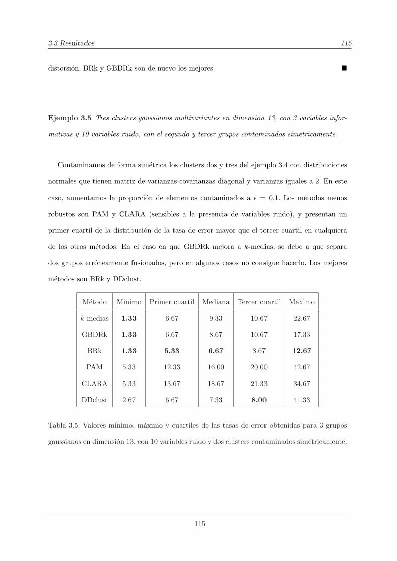
3.3 Resultados 115
distorsion, BRk y GBDRk son de nuevo los mejores. ¥
Ejemplo 3.5 Tres clusters gaussianos multivariantes en dimension 13, con 3 variables infor-
mativas y 10 variables ruido, con el segundo y tercer grupos contaminados simetricamente.
Contaminamos de forma simetrica los clusters dos y tres del ejemplo 3.4 con distribuciones
normales que tienen matriz de varianzas-covarianzas diagonal y varianzas iguales a 2. En este
caso, aumentamos la proporcion de elementos contaminados a ε = 0,1. Los metodos menos
robustos son PAM y CLARA (sensibles a la presencia de variables ruido), y presentan un
primer cuartil de la distribucion de la tasa de error mayor que el tercer cuartil en cualquiera
de los otros metodos. En el caso en que GBDRk mejora a k-medias, se debe a que separa
dos grupos erroneamente fusionados, pero en algunos casos no consigue hacerlo. Los mejores
metodos son BRk y DDclust.
Metodo Mınimo Primer cuartil Mediana Tercer cuartil Maximo
k-medias 1.33 6.67 9.33 10.67 22.67
GBDRk 1.33 6.67 8.67 10.67 17.33
BRk 1.33 5.33 6.67 8.67 12.67
PAM 5.33 12.33 16.00 20.00 42.67
CLARA 5.33 13.67 18.67 21.33 34.67
DDclust 2.67 6.67 7.33 8.00 41.33
Tabla 3.5: Valores mınimo, maximo y cuartiles de las tasas de error obtenidas para 3 grupos
gaussianos en dimension 13, con 10 variables ruido y dos clusters contaminados simetricamente.
115

116 Capıtulo 3. Refinamientos robustos de k-medias mediante profundidad
KM GBD BRk PAM CL DDc
010
2030
40
Figura 3.6: Diagramas de caja de las tasas de error obtenidas con los seis metodos para conjuntos
con 3 grupos gaussianos en dimension 13, con 10 variables ruido y dos clustes contaminados
de forma simetrica.
El hecho mas destacable del comportamiento de BRk es que, de nuevo, en todos los casos
en los que k-medias une dos grupos de manera erronea, el metodo de refinamiento consigue
separarlos, obviamente por ser independiente de los puntos iniciales que fueron escogidos en
k-medias. ¥
En resumen, podemos ver que en datos simulados, GBDRk produce mejores resultados que
k-medias en un pequeno numero de iteraciones, pero para algunos conjuntos de datos, serıa
interesante un comportamiento mejor, en el sentido de evitar los malos resultados en los que k-
116

3.3 Resultados 117
medias queda atascada y de separar grupos que han sido unidos incorrectamente, para conseguir
tasas de error menos variables. Por otra parte, BRk tiene en general un comportamiento muy
robusto, similar e incluso mejor en ocasiones al de DDclust, siendo estos dos los mejores de todos
los metodos utilizados. BRk consigue mejorar tanto la distorsion como la tasa de elementos
mal asignados en k-medias, y obtiene sus resultados en mucho menos tiempo que DDclust.
3.3.2. Resultados en datos reales
Aplicamos los seis metodos al conjunto de datos de expresion genica descrito en Golub et al.
(1999). Estos datos proceden de un estudio de las expresiones genicas en dos tipos de leucemia:
leucemia linfoblastica aguda (ALL) y leucemia mieloide aguda (AML). El estudio fue realizado
a partir de 25 casos de AML, y 47 casos de ALL (72 muestras en total). Los casos de ALL
consistıan en 38 muestras procedentes de celulas tipo B (ALL-B) y 9 de celulas de tipo T
(ALL-T). Las expresiones genicas se midieron en 6817 genes (humanos), de forma simultanea.
Redujimos el numero de genes en estudio a 3571 como en Dudoit y Fridlyand (2002) siguiendo
los siguientes pasos de pre-procesado. En primer lugar, se tomo una cota inferior de 100 y
una cota superior de 16000, y todas las medidas que estaban por debajo de la cota inferior
se sustituyeron por este valor, del mismo modo que las observaciones por encima de la cota
superior se truncaron a dicha cota; a continuacion, los datos se filtraron excluyendo aquellos
genes que presentaban una relacion senal-ruido baja, es decir, los que verificaban max/min ≤ 5
o (max−min) ≤ 500, donde max y min hacen referencia a las intensidades maxima y mınima,
respectivamente, de cada gen en las 72 muestras. Finalmente, estandarizamos los datos de
forma que cada muestra estuviese centrada en 0 y presentara varianza 1, para evitar que el
analisis estuviera dominado por algun experimento en particular, como se sugiere en Jornsten
et al. (2002). La mayor parte de los genes en este conjunto no estaban activos, por lo que
seleccionamos los 100 mas variables (en las muestras) antes de continuar con el analisis. De
117

118 Capıtulo 3. Refinamientos robustos de k-medias mediante profundidad
esta forma, el conjunto reducido consistıa en k = 3 grupos de muestras en dimension d = 100.
KM GBD BRk PAM CL DDc
510
1520
Figura 3.7: Diagramas de caja de las tasas de error obtenidas con los seis metodos en los datos
de leucemia.
Aplicamos 50 veces cada uno de los metodos al conjunto resultante para agrupar las muestras
en lugar de los genes; tanto PAM como CLARA produjeron siempre el mismo clustering, con
una tasa de error de 8.33%, que se corresponde con la asignacion incorrecta de 6 muestras (en
concreto, las etiquetadas con 28, 35, 38, 64, 66 y 67), de las cuales 5 corresponden a muestras
AML y una a una muestra ALL-T. DDclust produjo clusterings distintos, con tasas de error
entre 5.55 % y 8.33% (que corresponde a la asignacion incorrecta de entre 4 y 6 muestras). k-
medias obtuvo resultados mas variables, como se muestra en la figura 3.7, con la tasa de error
118

3.3 Resultados 119
oscilando entre 4.167 % y 23.61 % (de 3 a 17 muestras). GBDRk mejoro notablemente estos
resultados, haciendo caer la tasa de error en 9 de las 50 aplicaciones del metodo, y clasificando
mal 5 muestras en 34 casos, y 4 muestras en 10 casos. Observese que mas de la mitad de
las aplicaciones de k-medias produjeron un porcentaje de elementos mal asignados menor o
igual que 6.944% (5 muestras), lo cual permite a BRk formar, en media, clusters de centros
compactos en los que buscar los puntos iniciales. Por tanto, los resultados de BRk son mucho
mas satisfactorios que los de k-medias, obteniendo un numero de muestras mal asignadas mayor
que 5 en solo 4 de las 50 aplicaciones del metodo. Sin embargo, esto no es mucho mejor que lo
obtenido por GBDRk, el cual asignaba mal mas de 5 muestras en solo 6 de los 50 casos. DDclust
es el metodo que proporciona mejores resultados en este conjunto, con un valor maximo para
la tasa de error significativamente mas bajo que en los otros algoritmos.
Metodo Mınimo Primer cuartil Mediana Tercer cuartil Maximo
k-medias 4.167 6.944 6.944 16.319 23.611
GBDRk 4.167 6.944 6.944 6.944 23.611
BRk 4.167 6.944 6.944 6.944 20.833
PAM 8.333 8.333 8.333 8.333 8.333
CLARA 8.333 8.333 8.333 8.333 8.333
DDclust 5.555 5.555 6.249 6.944 8.333
Tabla 3.6: Valores mınimo, maximo y cuartiles de las tasas de error obtenidas para los datos
de leucemia.
Para estudiar el impacto producido por el numero de variables incluidas en la precision
de los clusters, todos los procedimientos fueron aplicados a los datos de leucemia usando los
p = 500 y 1000 genes con mayor varianza en las muestras. El comportamiento de PAM y
119

120 Capıtulo 3. Refinamientos robustos de k-medias mediante profundidad
CLARA se deterioro al incluir variables ruido (genes no informativos), aumentando el numero
de muestras mal asignadas de 6 a 7 y 13, respectivamente, lo cual es consistente con los
resultados obtenidos en nuestro estudio de simulacion. Por otra parte, el comportamiento de
los otros cuatro metodos permanece estable, siendo DDclust el mas preciso, seguido por BRk
y GBDRk. k-medias mostro la misma dispersion en la tasa de error que en el caso de p = 100
genes. ¥
En resumen, en esta seccion hemos propuesto dos metodos diferentes para encontrar las
semillas iniciales del algoritmo de k-medias que mejoran considerablemente sus resultados. El
primero, basado en la busqueda del dato mas profundo de cada cluster de los encontrados
por k-medias, obtiene buenos resultados en general, pero en algunas ocasiones no es capaz de
descartar mınimos locales en los que k-medias se queda atrapada. El segundo, que combina
bootstrap con la busqueda del dato mas profundo de cada cluster (compacto) de centroides
bootstrap, soluciona este problema, obteniendo resultados robustos que son comparables a los
obtenidos por DDclust, otro metodo de clustering robusto y basado en profundidad de datos,
pero con la ventaja de ser mas rapido que este.
El comportamiento del metodo de refinamiento basado en encontrar el dato mas profundo
de cada cluster bootstrap para formar el conjunto D, con k ·B elementos, y en agrupar dicho
conjunto en clusters, sera objeto de investigacion futura.
120

3.4 Clustering no rıgido basado en bootstrap 121
3.4. Clustering no rıgido basado en bootstrap
Los algoritmos de clustering estandar que hemos usado hasta el momento asignan genes a
clusters basandose en la similaridad de sus patrones de actividad. Genes con patrones simi-
lares deberıan ser agrupados juntos, mientras que genes con distintos patrones de activacion
deberıan ser colocados en clusters diferentes. Estos metodos de clustering estan restringidos
a correspondencias “uno-a-uno”: un gen corresponde exactamente a un cluster. Mientras que
este principio parece razonable en muchos campos del analisis cluster, puede resultar demasiado
limitado para el estudio de datos procedentes de microarrays. Los genes pueden participar en
diferentes redes geneticas y son coordinados frecuentemente por una gran variedad de mecanis-
mos de regulacion. Para el analisis de datos de microarrays, por tanto, podemos esperar que un
gen pertenezca a varios clusters. Diversos investigadores han hecho notar que existen genes que
frecuentemente estan altamente correlados con multiples grupos y que la definicion de fronteras
nıtidas entre clusters de datos de expresiones genicas a menudo resulta arbitraria (Chu et al.,
1998; Cho et al., 1998). Esto motiva el uso de tecnicas tales como el algoritmo de c-medias
difuso (FCM), introducido por Bezdek (1981).
En Teorıa del Aprendizaje, el clustering difuso es una tecnica que establece particiones en
los datos, pero que permite pertenencias parciales, es decir, grados de pertenencia entre 0
y 1 en lugar de asignaciones rıgidas de los datos a los clusters. Estas tecnicas pertenecen a
las tecnicas de computacion difusa, las cuales incluyen redes neuronales, sistemas difusos y
algoritmos geneticos. En este sentido, el clustering no rıgido que presentamos a continuacion
se puede considerar proximo a alguno de los algoritmos de este campo. Como ejemplo, vease
Grotkjaer et al. (2006).
121

122 Capıtulo 3. Refinamientos robustos de k-medias mediante profundidad
Consideramos que U es una particion no rıgida del conjunto X si puede ser definida a traves
de una matriz de pertenencias cuyas celdas estan confinadas en el intervalo unidad, y que
satisface los dos requisitos siguientes (Pedrycz, 2005):
a) Los clusters son no triviales: para cada cluster obtenemos una estructura en la
matriz que no incluye todos los datos.
b) Los grados de pertenencia totales suman 1.
El metodo presentado en la seccion 3.2.3 permite la construccion de una particion no rıgida
de los datos que en ocasiones puede ser mas apropiada para agrupar un conjunto dado. Con-
sideremos el conjunto de centros C = {Cbi , i = 1, ..., k, b = 1, ..., B} obtenido en el paso 3 del
algoritmo BRk, que es agrupado para obtener k clusters I∗1 , ..., I∗k . Podemos construir una re-
gion de confianza para las semillas iniciales, que recordemos que se calculaban como los puntos
mas profundos Di en cada cluster I∗i , eliminando primero los puntos con menor profundidad
hasta que se alcanza el tamano deseado, y formando a continuacion la envolvente convexa de los
puntos restantes como se describe en Yeh y Singh (1997). Denotaremos por W ∗1−α(Di) la region
obtenida al eliminar los 100α % puntos bootstrap mas externos de I∗i , usando la profundidad
por bandas generalizada, y por H(A) la envolvente convexa de un conjunto A.
Consideremos k puntos distintos en Rd, y1, . . . , yk. Las regiones de Voronoi de los puntos
y1, . . . , yk (ver, por ejemplo, de Berg et al. (2000)), o los dominios de atraccion para los
puntos yi, i = 1, ..., k, se definen como:
A(yi) = {x ∈ Rd : d(x, yi) < d(x, yj), i 6= j}.
122

3.4 Clustering no rıgido basado en bootstrap 123
Las regiones de Voronoi de un conjunto de k puntos distintos crean una particion con k
regiones o celdas convexas de Rd. El algoritmo de k-medias consiste en encontrar las regiones
de Voronoi de los k centroides. Vease la figura 3.8.a). Observese que los puntos que se encuentran
en las fronteras de las celdas se asignan arbitrariamente a uno de los clusters adyacentes.
a) b)
Figura 3.8: a) Ocho clusters con los correspondientes centros (medias) dibujados en rojo. Las
regiones de Voronoi convexas (polıgonos) estan delimitadas por lıneas azules. b) Regiones de
Voronoi generalizadas no convexas relativas a los dominios de atraccion de tres triangulos
distintos.
Consideremos los k puntos mas profundos Di obtenidos en el metodo BRk, asumiendo
que son distintos. El dominio de atraccion del punto Di se puede generalizar a otros lugares
geometricos, y en particular, el dominio de atraccion de la envolvente convexa del conjunto
W ∗1−α(Di) esta dado por
A(H(W ∗1−α(Di))) = {x ∈ Rd : d(x,H(W ∗
1−α(Di))) < d(x,Dj), i 6= j},
123

124 Capıtulo 3. Refinamientos robustos de k-medias mediante profundidad
donde la distancia de un punto x a un conjunto A esta definida por
d(x,A) = mina∈Ad(x, a).
Esto determina una particion de Voronoi generalizada del espacio, con regiones que en
general no son convexas, y que conduce por tanto a una agrupacion diferente de los datos de
la dada por k-medias.
Proposicion 3.2 El dominio de atraccion generalizado de la envolvente convexa de W ∗1−α(Di)
contiene las regiones de Voronoi de Di.
Demostracion: Es inmediato teniendo en cuenta que Di es el punto mas profundo de I∗i y
por tanto, para cada α, Di ∈ W ∗1−α(Di). De aquı, si z ∈ A(Di), d(z,Di) < d(z,Dj), j 6= i y por
tanto d(z, H(W ∗1−α(Di))) ≤ d(z,Di) < d(z,Dj), j 6= i. ¥
La proposicion 3.2 justifica el siguiente metodo para generar un clustering no rıgido del
conjunto X. Construiremos las regiones de Voronoi generalizadas de los lugares geometricos
(distintos) D1, . . . ,Di−1, W ∗1−α(Di),Di+1, . . . ,Dk, para cada i = 1, ..., k. La interseccion de las
k particiones origina 2k − 1 regiones disjuntas, que en general no son convexas, algunas de las
cuales pueden ser vacıas, y que se pueden describir como sigue:
I(k) =k⋂
i=1
A(H(W ∗1−α(Di)))
I(k−1)j =
⋂
i6=j
A(H(W ∗1−α(Di)))− I(k), j = 1, ..., k
124

3.4 Clustering no rıgido basado en bootstrap 125
I(k−2)j1,j2
=⋂
i6=j1,j2
A(H(W ∗1−α(Di)))− I(k) −
k⋃
j=1
I(k−1)j , j1 6= j2
...
I(1)j1,...,jk−1
= A(H(W ∗1−α(Djk
)))− I(k) − ...−⋃
I(2)j1,...,jk−1
, jk = 1, ..., k
En ocasiones nos referiremos genericamente a estas regiones sin mencionar los subındices.
Los puntos que pertenecen a I(1)j1,...,jk−1
son los que no han sido atraıdos por ningun otro centro
o su correspondiente region de confianza aparte de Djk. En la figura 3.9 podemos ver las 7 re-
giones, I(3), I(2)1 , I
(2)2 , I
(2)3 , I
(1)1,2 , I
(1)1,3 y I
(1)2,3 , originadas al calcular las tres particiones de Voronoi
generalizadas correspondientes a dos puntos y un triangulo (que representa la envolvente con-
vexa de la region de confianza del tercer punto). Estas regiones estan limitadas por lıneas azules
discontinuas. Las lıneas negras continuas son las fronteras de los dominios de atraccion de los
puntos D1, D2 y D3.
Las regiones de Voronoi de los puntos D1, . . . ,Dk determinan una particion C1, . . . , Ck del
conjunto X que puede ser descrita en terminos de probabilidades como sigue:
P0{x ∈ Ci} =
1, si x ∈ A(Di)
1h si x ∈ δ(A(Di))
0, en otro caso,
donde δ(A) representa la frontera del conjunto A y h es el numero de celdas de Voronoi cuyas
fronteras incluyen al punto x.
125

126 Capıtulo 3. Refinamientos robustos de k-medias mediante profundidad
Figura 3.9: Siete regiones disjuntas correspondientes a las tres particiones de Voronoi genera-
lizadas para dos puntos y un triangulo. Las fronteras de estas regiones son las lıneas azules
discontinuas. Las fronteras de las regiones de Voronoi “estandar” correspondientes a los tres
puntos estan representadas por lıneas negras continuas.
Para un tamano dado 100(1−α) % de las regiones de confianza bootstrap, podemos definir
una particion no rıgida del conjunto X en clusters F1, . . . , Fk, generada por los centros D1,...,Dk,
y descrita por las siguientes probabilidades: primero, si x esta en la frontera de algun A(Di)
entonces es asignado arbitrariamente a cualquiera de los clusters adyacentes; segundo, si x
esta en cualquiera de las k regiones I(1), entonces la probabilidad de pertenecer al cluster Fi
126

3.4 Clustering no rıgido basado en bootstrap 127
esta dada por:
Pα{x ∈ Fi} = P0{x ∈ Ci}
y, finalmente, si x esta en cualquiera de las otras regiones I(q)j1,...,jk−q
− ∪iδ(A(Di)), q > 1, la
probabilidad de pertenecer al cluster Fi esta dada por:
Pα{x ∈ Fi} =
1q
+α
q, si x ∈ A(Di), i 6= j1, ..., jk−q
1q− α
q(q − 1), si x /∈ A(Di), i 6= j1, ...jk−q
0, en otro caso.
(3.4.3)
Ası, si un punto no es atraıdo por otro centro o region de confianza aparte de Di, entonces
sera asignado al cluster Fi con probabilidad 1. La probabilidad de asignacion de los restantes
puntos tiene en cuenta a las regiones de confianza que los atraen. A los puntos en las fronteras
se les asigna arbitrariamente la probabilidad de pertenencia correspondiente a cualquiera de
las regiones adyacentes.
Pα(.) y, en particular, la funcion de probabilidad (3.4.3) esta bien definida, como se demues-
tra a continuacion.
Proposicion 3.3 Si un punto x ∈ I(q)j1,...,jk−q
entonces x /∈ A(Dj), j = j1, ..., jk−q.
Demostracion: En efecto, si x ∈ I(q)j1,...,jk−q
y x ∈ A(Dg), para algun g ∈ {j1, ..., jk−q},
127

128 Capıtulo 3. Refinamientos robustos de k-medias mediante profundidad
entonces x ∈ A(H(W ∗1−α(Dg))), y x ∈
⋂
i6=j1,...,jk−q
A(H(W ∗1−α(Di))) ∩ A(H(W ∗
1−α(Dg)))
.
Por tanto, existe un entero positivo l tal que x ∈ I(q+l) y x /∈ I(q)j1,...,jk−q
, lo cual no es posible.
Ası, x /∈ A(Dg), ∀g ∈ {j1, ..., jk−q}. ¥
Por consiguiente, si x /∈ δ(A(Di)) para algun i, entonces pertenece a algun A(Di), i 6=
j1, ..., jk−q, y (3.4.3) esta bien definida.
Proposicion 3.4 Los grados de pertenencia dados por Pα{x ∈ Fi} suman 1.
Demostracion: Trivialmente, si x ∈ I(1) o x ∈ δ(A(Dj)) para algun j, entoncesk∑
i=1
Pα{x ∈
Fi} = P0{x ∈ Ci} = 1.
Por otra parte, si x ∈ I(q)j1,...,jk−q
− ∪iδ(A(Di)), q > 1, entonces ∃s 6= j1, ..., jk−q tal que
x ∈ A(Ds). Por tanto,
k∑
i=1
Pα{x ∈ Fi} =∑
i=j1,...,jk−q
Pα{x ∈ Fi}+∑
i6=j1,...,jk−q
Pα{x ∈ Fi} = 0 + Pα{x ∈ A(Ds)}+
+∑
i 6=j1,...,jk−q ,s
Pα{x ∈ A(Di)} =1q
+α
q+ (q − 1)
(1q− α
q(q − 1)
)=
q
q= 1. ¥
La figura 3.10 muestra las probabilidades de asignacion de tres clusters no rıgidos, codificados
por colores. Las probabilidades de los puntos en las fronteras de las regiones de Voronoi no se
muestran.
El inconveniente practico de este metodo es el coste computacional de las regiones de Voronoi
para datos de alta dimension. Sin embargo, existen algoritmos aproximados que calculan tales
128

3.4 Clustering no rıgido basado en bootstrap 129
Figura 3.10: Probabilidades de asignacion de un punto x a cada uno de los tres clusters no
rıgidos, codificados por colores. Cuanto mas proximo este el color correspondiente al rojo, azul
o amarillo puros, mayor sera la probabilidad de pertenecer a uno de estos clusters.
regiones y que pueden ser utilizados para acelerar los calculos. Vease, por ejemplo, Hoff et al.
(1999) y las referencias contenidas en este trabajo.
129

130 Capıtulo 3. Refinamientos robustos de k-medias mediante profundidad
3.4.1. Resultados en los datos de leucemia
Comprobamos el metodo propuesto en los datos de leucemia para determinar un clus-
tering no rıgido de las 72 muestras. Considerando tres posibles clusters, ALL-B, ALL-T y
AML, podemos construir 7 regiones de Voronoi generalizadas (aproximadas) en dimension
d = 100. Tras asignar las 72 muestras en estas regiones, encontramos que 49 de las 72 muestras
pertenecıan a una de las regiones I(1), y que todas ellas estaban bien clasificadas; 12 muestras
pertenecıan a algunas de las regiones I(2) y 11 de ellas pertenecıan a I(3). La distribucion del
numero de muestras en las siete regiones del espacio 100-dimensional esta dada en la tabla 3.7.
Las 5 muestras que habıan sido mal clasificadas con el metodo BRk (muestras 28, 35, 38 y 66,
de tipo AML y la muestra 67, de tipo ALL-T) pertenecen a las regiones I(3). Las probabilidades
de pertenencia dadas por el metodo se recogen en la tabla 3.8.
Tipo de tumor I(1)2,3 I
(1)1,3 I
(1)1,2 I
(2)3 I
(2)2 I
(2)1 I(3)
ALL-B 28 0 0 6 2 0 2
ALL-T 0 6 0 0 0 0 3
AML 0 0 15 3 0 1 6
Tabla 3.7: Distribucion de las muestras en las regiones de Voronoi.
Este conjunto de datos reales muestra que incluso si algunas muestras no se asignan de
forma unica a un cluster, el metodo es capaz de identificar aquellas muestras que habıan sido
mal clasificadas usando un algoritmo de clustering estandar, y de asignarle una probabilidad
balanceada de pertenecer a cada cluster.
130

3.4 Clustering no rıgido basado en bootstrap 131
Probabilidad ALL-B ALL-T AML Grupo real
Muestra 28 0.35 0.325 0.325 AML
Muestra 35 0.35 0.325 0.325 AML
Muestra 38 0.325 0.35 0.325 AML
Muestra 66 0.35 0.325 0.325 AML
Muestra 67 0.35 0.325 0.325 ALL-T
Tabla 3.8: Probabilidades de pertenencia a cada uno de los clusters formados por las muestras
de los tres tipos de tumor. ¥
131

132 Capıtulo 3. Refinamientos robustos de k-medias mediante profundidad
132

Capıtulo 4
Estimacion del numero de grupos
Resumen
Como se menciono previamente, un aspecto esencial del problema de clustering que deberıa
ser abordado antes de utilizar un metodo particular en un conjunto de datos dado es la esti-
macion del numero de grupos subyacentes, si existe alguno. En este capıtulo presentamos un
estudio disenado para estimar el numero de grupos en la estructura de los datos, aprovechando
el algoritmo greedy utilizado en el metodo de comparacion de clusterings, descrito en la sec-
cion 2.2.1, y la definicion de profundidad empleada en el capıtulo anterior. En el primer caso,
dependiendo del numero de clusters usados en cada comparacion, proponemos dos enfoques,
el k-unico (single k) y el k-mixto (mixed k). En el segundo caso, usamos ideas previas acerca
del diametro de un conjunto, combinadas con la nocion de profundidad. Encontramos que el
metodo k-unico proporciona una estimacion razonable del rango en el cual utilizar el metodo
k-mixto, y para una gran variedad de conjuntos de datos, la estimacion basada en los diametros
y en la profundidad proporciona un valor preciso del numero de grupos.
133

134 Capıtulo 4. Estimacion del numero de grupos
4.1. Introduccion
Como se menciono anteriormente, el clustering es una tecnica de aprendizaje no supervisado
en el cual se trata de encontrar una serie de grupos sin la ayuda de una variable respuesta.
Uno de los mayores retos en el analisis cluster es la estimacion del numero de grupos en un
conjunto dado, lo cual es esencial para realizar una agrupacion de los datos efectiva y eficiente.
Por ejemplo, un algoritmo de clustering como k-medias puede generar una mala agrupacion
si las particiones iniciales no son escogidas de forma apropiada, una situacion que ocurre a
menudo y cuya solucion no es una tarea trivial.
Se han propuesto muchos metodos para estimar el numero de grupos. Como se dijo en la
introduccion, algunas propuestas que se han usado en datos de expresion genica, o que han
sido expresamente disenadas para este tipo de datos son las siguientes:
el estadıstico “silueta”, propuesto en Kaufman y Rousseeuw (1990). Dada una
observacion i sea a(i) la distancia media de este punto a las otras observaciones del
mismo cluster, y sea b(i) la distancia media del punto a las observaciones del cluster
mas proximo (descartando el propio). Entonces, se define el estadıstico silueta como
s(i) =b(i)− a(i)
max{a(i), b(i)} .
Un punto esta bien asignado si s(i) toma un valor alto. Los autores proponen
escoger como numero optimo de clusters el valor que maximiza la media de los s(i)
en el conjunto completo, sil =∑
i
s(i)n
.
Observese que s(i) no esta definido para k = 1 cluster.
134

4.1 Introduccion 135
el estadıstico gap, propuesto en Tibshirani et al. (2001). Este metodo compara
la suma de cuadrados intra-clusters con su esperanza bajo una distribucion nula
de referencia como se explica a continuacion. Para cada numero posible de clusters
k ≥ 1, se calcula la suma de cuadrados intra clusters trWk. Se generan B conjuntos
de referencia bajo la distribucion nula y se aplica el algoritmo de clustering a cada
uno de ellos, calculando las correspondientes sumas de cuadrados intra-clusters
trW 1k ,...,trWB
k . Finalmente, se calcula el estadıstico gap estimado como:
gap(k) =1B
∑
b
logtrW bk − logtrWk
y la desviacion estandar sdk de trW bk , 1 ≤ b ≤ B. Sea sdk = sdk
√1 + 1/B. El
numero de clusters estimado es el menor k ≥ 1 tal que
gap(k) ≥ gap(k + 1)− sdk+1.
Tibshirani et al. eligieron la hipotesis de uniformidad para crear la distribucion
nula de referencia, y consideraron dos posibles maneras de construir la region de
soporte de tal distribucion. En la primera posibilidad, la ventana de muestreo
para la j-esima variable (1 ≤ j ≤ d) se limita al rango de los valores observados
en esta variable. En la segunda opcion, las variables se muestrean a partir de
una distribucion uniforme confinada a una “caja” alineada con las componentes
principales de la matriz del diseno, centrada. En detalle, si X es la matriz de datos,
supongamos que las columnas tienen media cero y calculemos la descomposicion
en valores singulares X = UDV T . Transformamos via X ′ = XV y a continuacion
obtenemos las variables uniformes Z ′ en los rangos de las correspondientes columnas
de X ′. Finalmente, se deshace la transformacion en la nueva matriz de diseno vıa
135

136 Capıtulo 4. Estimacion del numero de grupos
Z = Z ′V T para obtener el conjunto de referencia. Este segundo enfoque se denota
por gapPC, donde PC corresponde a las Componentes Principales. Observese que,
en este caso, el metodo sı permite la estimacion de k = 1 cluster.
el metodo CLEST, introducido por Dudoit y Fridlyand (2002). El algoritmo con-
siste en dividir repetidamente la muestra en un conjunto de entrenamiento Lb y
un conjunto de validacion T b. Para cada iteracion y para cada posible numero
de clusters k se obtiene un clustering P (·, Lb) del conjunto de entrenamiento y se
construye un predictor C(·, T b) usando las etiquetas de las clases obtenidas en el
clustering. A continuacion, se aplica el predictor al conjunto de validacion y las
etiquetas predichas se comparan con las obtenidas al agrupar (con algun metodo
de clustering) los datos del conjunto de validacion, usando algun estadıstico de
similaridad (por ejemplo, el ındice de Rand). El numero de clusters se estima com-
parando el estadıstico de similaridad observado para cada k con su valor esperado
bajo alguna distribucion nula apropiada con k = 1. El numero estimado de clusters
se define como el k que proporciona mayor evidencia en contra de la hipotesis nula.
el estadıstico ReD, propuesto por Jornsten (2004) y basado en la nocion de pro-
fundidad. Es muy similar al estadıstico silueta. Para una observacion i, ReDi es la
diferencia entre las profundidades con respecto al cluster en el cual ha sido asignada,
denotada por Dwi , y el cluster mas proximo, denotado por Db
i . El numero de clus-
ters seleccionado por el estadıstico ReD es el valor k que maximiza la profundidad
relativa media ReD =∑
i
ηiReDi, donde ηi es la multiplicidad de la observacion i.
A diferencia de sil, ReD es independiente de las escalas de los clusters, por lo que
136

4.2 Comparacion de pares de clusterings 137
no esta dominado por clusters de gran varianza.
En este capıtulo proponemos dos metodos para estimar el numero de grupos de un conjunto;
el primero toma ideas del metodo de comparacion de clusterings descrito en el capıtulo 2; el
segundo es un metodo muy simple, basado en seleccionar subconjuntos de cada cluster, o mas
precisamente, los α % puntos mas profundos en el clusters, y en calcular la suma de los diametros
de tales subconjuntos. De nuevo, la nocion de profundidad que usaremos en este capıtulo es la
profundidad por bandas generalizadas descrita en Lopez-Pintado y Romo (2006).
4.2. Comparacion de pares de clusterings
El algoritmo greedy propuesto en el capıtulo 2 conduce de manera natural al problema
de estudiar la distribucion del numero de super-clusters que resultan al comparar un par de
clusterings del mismo conjunto de datos. La dificultad de este estudio, que deriva de la ausen-
cia general de resultados distribucionales relacionados con los algoritmos de clustering, y en
particular con k-medias, sugiere el uso de tecnicas bootstrap.
Para un conjunto dado X con N elementos, extraıdo de una poblacion con k clusters, es
posible encontrar la distribucion bootstrap del numero de super-clusters p, suponiendo que
hemos aplicado dos veces k-medias a X, iniciando con k clusters, en los pasos siguientes:
1. FOR i in 1:B DO
1.1 Obtener una muestra bootstrap X∗i de X con N elementos.
1.2 Aplicar k-medias dos veces a X∗i para obtener los clusterings A∗
i y B∗i , cada uno
con k grupos.
137

138 Capıtulo 4. Estimacion del numero de grupos
1.3 Usar el algoritmo greedy para calcular el numero de super-clusters p∗i .
2. Calcular la distribucion bootstrap del numero de super-clusters p.
3. Estimar p con la moda de esta distribucion bootstrap.
Denotemos a los centros de los k grupos de la poblacion de la cual ha sido extraıdo X por
µ1, . . . , µk. Supongamos que aplicamos k-medias con k clusters a X y obtenemos el clustering
A = {A1, . . . , Ak}, y denotemos a los correspondientes centros de los clusters por {a1, . . . , ak}.
Si se verifican las condiciones del teorema de Pollard, expuesto en Pollard (1982), entonces los
centros muestrales convergen a los centros poblacionales µ1, . . . , µk, salvo por reordenacion de
los ındices, y por tanto, cuando el tamano muestral es suficientemente grande, el numero de
super-clusters converge al numero real de grupos, k.
Desafortunadamente, este razonamiento falla en la practica, pues habitualmente el numero
de grupos es desconocido, y ademas tampoco se conocen resultados distribucionales teoricos
para k-medias cuando el numero de clusters utilizado al aplicar el metodo es diferente del k de
la poblacion; por supuesto, el mismo procedimiento anterior puede ser utilizado para calcular la
distribucion bootstrap del numero de super-cluster para dos clusterings dados con un numero
de clusters diferente al de la poblacion k, pero no podemos esperar que p converja a k. Ası,
en los casos practicos en los que el numero de grupos k es desconocido, no podremos utilizar p
como un estimador preciso de k. Para ilustrar como se incrementa el valor de p cuando variamos
el numero de clusters utilizado en k-medias, consideremos las siguientes simulaciones.
Ejemplo 4.1 Modelo 1.
138

4.2 Comparacion de pares de clusterings 139
Generamos diversos conjuntos de datos segun el modelo 1, con 4 grupos, nivel de ruido σ = 4
y distintos tamanos para los clusters c1 = c2 = c3 = c4 = i, siendo i = 25, 50, 100, 200 y 500,
y a continuacion calculamos la distribucion bootstrap de p al usar k-medias con 4, 5, 6 y 7
clusters.
1 2 3 4
0,00
0,25
0,50
0,75
1,00
Boo
tstr
ap fr
eque
ncy
Number of superclustersModel 1, 4 clusters, σσσσ = 4
Cluster size = 25 Cluster size = 50 Cluster size = 100 Cluster size = 200 Cluster size = 500
Figura 4.1: Modelo 1 con 4 clusters, σ = 4 y diferentes tamanos de los clusters. Distribucion
bootstrap de p cuando se aplica k-medias con 4 clusters.
Para 4 clusters, se observa claramente que, al aumentar el tamano de los clusters, la fre-
cuencia de los 4 super-clusters aumenta tambien, tal y como esperabamos. Para 5 clusters, la
distribucion bootstrap de p tiene tambien una clara moda en 4 para todos los tamanos de los
clusters, pero no es el caso de 6 y 7 clusters. Para 6 clusters y los tamanos de clusters mas
pequenos, la moda sigue siendo 4, pero para tamanos a partir de 200 es igualmente probable
encontrar 4 o 5 super-clusters. Finalmente, para 7 clusters, la moda es 5. Aunque no mostramos
los resultados aquı, hemos observado que a medida que el numero de clusters aumenta, la moda
de la distribucion bootstrap se aleja cada vez mas de 4.
139

140 Capıtulo 4. Estimacion del numero de grupos
1 2 3 4 5
0,00
0,25
0,50
0,75
1,00
Boo
tstr
ap fr
eque
ncy
Number of superclusters (k=5)Model 1, 4 clusters, σσσσ = 4
Cluster size = 25 Cluster size = 50 Cluster size = 100 Cluster size = 200 Cluster size = 500
Figura 4.2: Modelo 1 con 4 clusters, σ = 4 y diferentes tamanos de los clusters. Distribucion
bootstrap de p cuando se aplica k-medias con 5 clusters.
1 2 3 4 5 6
0,00
0,25
0,50
0,75
1,00
Boo
tstr
ap fr
eque
ncy
Number of superclusters (k=6)Model 1, 4 clusters, σσσσ = 4
Cluster size = 25 Cluster size = 50 Cluster size = 100 Cluster size = 200 Cluster size = 500
Figura 4.3: Modelo 1 con 4 clusters, σ = 4 y diferentes tamanos de los clusters. Distribucion
bootstrap de p cuando se aplica k-medias con 6 clusters.
140

4.2 Comparacion de pares de clusterings 141
1 2 3 4 5 6 7
0,00
0,25
0,50
0,75
1,00
Boo
tstr
ap fr
eque
ncy
Number of superclusters (k=7)Model 1, 4 clusters, σσσσ = 4
Cluster size = 25 Cluster size = 50 Cluster size = 100 Cluster size = 200 Cluster size = 500
Figura 4.4: Modelo 1 con 4 clusters, σ = 4 y diferentes tamanos de los clusters. Distribucion
bootstrap de p cuando se aplica k-medias con 7 clusters. ¥
Ejemplo 4.2 Modelo 2.
Usamos conjuntos generados segun el modelo 2, tomando como tamanos de los clusters c1 =
c2 = 12c3 = i, siendo i = 25, 50, 100, 200 y 500, y a continuacion calculamos la distribucion
bootstrap de p al aplicar k-medias con 3, 4, 5 y 6 clusters.
Como ocurre en el ejemplo anterior, en los casos en los que aplicamos k-medias con 3 y 4
clusters, la distribucion bootstrap del numero de super-clusters tiene una sola moda en 3, el
verdadero numero de grupos; sin embargo, cuando el numero de clusters aumenta, la moda
tambien aumenta, como se puede observar en las figuras 4.5, 4.6, 4.7 y 4.8.
141

142 Capıtulo 4. Estimacion del numero de grupos
1 2 3
0,00
0,25
0,50
0,75
1,00
Boo
tstr
ap d
istr
ibut
ion
Number of superclusters (k=3)Model 2, 3 clusters
Cluster size = 25 Cluster size = 50 Cluster size = 100 Cluster size = 200 Cluster size = 500
Figura 4.5: Modelo 2 con 3 clusters y diferentes tamanos de los clusters. Distribucion bootstrap
de p al aplicar k-medias con 3 clusters.
1 2 3 4
0,00
0,25
0,50
0,75
1,00
Boo
tstr
ap d
istr
ibut
ion
Number of superclusters (k=4)Model 2, 3 clusters
Cluster size = 25 Cluster size = 50 Cluster size = 100 Cluster size = 200 Cluster size = 500
Figura 4.6: Modelo 2 con 3 clusters y diferentes tamanos de los clusters. Distribucion bootstrap
de p al aplicar k-medias con 4 clusters.
142

4.2 Comparacion de pares de clusterings 143
1 2 3 4 5
0,00
0,25
0,50
0,75
1,00
Boo
tstr
ap d
istr
ibut
ion
Number of superclusters (k=5)Model 2, 3 clusters
Cluster size = 25 Cluster size = 50 Cluster size = 100 Cluster size = 200 Cluster size = 500
Figura 4.7: Modelo 2 con 3 clusters y diferentes tamanos de los clusters. Distribucion bootstrap
de p al aplicar k-medias con 5 clusters.
1 2 3 4 5 6
0,00
0,25
0,50
0,75
1,00
Boo
tstr
ap d
istr
ibut
ion
Number of superclusters (k=6)Model 2, 3 clusters
Cluster size = 25 Cluster size = 50 Cluster size = 100 Cluster size = 200 Cluster size = 500
Figura 4.8: Modelo 2 con 3 clusters y diferentes tamanos de los clusters. Distribucion bootstrap
de p al aplicar k-medias con 6 clusters. ¥
143

144 Capıtulo 4. Estimacion del numero de grupos
Estos resultados y los obtenidos en la seccion 2.2.2, donde realizamos la comparacion de clus-
terings con distinto numero de clusters, muestran que no podemos esperar estimar el numero
de grupos de la poblacion k con el numero de super-clusters obtenido tras comparar dos clus-
terings con un numero cualquiera de clusters, pero sı son utiles para disenar un heurıstico para
estimar k basandonos en multiples comparaciones entre clusterings.
4.2.1. Muestreo en una poblacion de clusterings
La idea basica es la siguiente: comenzando con una “poblacion” de clusterings no jerarquicos
obtenidos en un mismo conjunto de datos X, realizamos sucesivas comparaciones entre pares de
dichos clusterings. La comparacion de cada par conduce a un nuevo par de clusterings con un
mismo numero de clusters p. Estas comparaciones unen la informacion acerca de como se pueden
agrupar los elementos de un conjunto, e intentan encontrar un consenso en una agrupacion
nueva. De esta manera, se espera que grupos reales que se dividieron incorrectamente en algunas
de las particiones iniciales –por ejemplo, porque el numero de clusters k utilizado en el algoritmo
de clustering era mayor que el numero real de grupos– se unan tras comparar el correspondiente
clustering con otros en los que esos grupos no habıan sido separados. Ası, si genes que en
algunas particiones pertenecen a diferentes clusters se agrupan juntos de manera persistente
tras comparar diversos clusterings, asumiremos que efectivamente pertenecen a un mismo super-
cluster, y por otra parte, si genes que pertenecen a clusters distintos en algunas particiones
siguen estando separados despues de la mayor parte de las comparaciones, asumiremos que no
comparten el mismo perfil y que por tanto deben permanecer en grupos diferentes.
Esta metodologıa tiene el inconveniente de ser totalmente dependiente de la calidad de
los clusterings utilizados como poblacion. En todas nuestras simulaciones hemos empleado k-
144

4.2 Comparacion de pares de clusterings 145
medias; como explicamos en la introduccion, existen otros metodos, como el algoritmo PAM
Kaufman y Rousseeuw (1990), que han demostrados ser mas robustos y eficientes que k-medias.
Ademas, este metodo tiene la ventaja adicional de proporcionar un grafico, la representacion
del estadıstico silueta, que puede utilizarse para seleccionar el numero de clusters optimo. La
razon por la que a pesar de ello utilizamos k-medias en nuestra intencion de estimar el numero
de grupos es que, siguiendo la lınea de refinamiento del capıtulo 3, pretendemos mejorar, al
mismo tiempo, la falta de robustez de los resultados obtenidos con k-medias usando las sucesivas
comparaciones.
De manera mas precisa, consideremos que la particion real de los datos en k grupos (k ≥ 1)
esta descrita por Creal y sea C una particion obtenida por algun procedimiento de clustering.
Si representamos ambas colecciones de clusters como nodos en un bigrafo, tal y como hicimos
en el capıtulo 2, y aplicamos el algoritmo greedy, obtendremos p componentes conexas. Si p
= k, diremos que C es una “buena” particion de X; en caso contrario, (i.e. p < k) diremos
que C es una “mala particion”, puesto que no es capaz de separar algunos de los grupos reales
(vease la figura 4.9.a).
Cuando dos particiones C1 y C2, con m y n clusters respectivamente, se comparan mediante
el algoritmo greedy, las dos particiones resultantes tendran p ≤ mın{m,n} clusters. Si tanto C1
como C2 son “buenas” particiones, lo mas comun es que las nuevas particiones tambien sean
“buenas”; en cambio, si alguna de las particiones une dos grupos reales en un unico cluster,
tras la comparacion, las dos nuevas particiones tambien lo haran (ver las figuras 4.9.b y c).
Existen casos en los que la comparacion de un clustring “malo” y otro “bueno” no hace que
el segundo se contamine. Por ejemplo, consideremos una particion real Creal con dos grupos,
y un par de clusterings, uno “bueno” y otro “malo”. Supongamos que el “mal” clustering A
145

146 Capıtulo 4. Estimacion del numero de grupos
Dos nuevas particiones con 3 clusters (malos clusterings)
Dos nuevas particiones con 2 clusters (malos clusterings)
La partición azul es un buen clustering (4 componentes conexas)
Las particiones rojas son malos clusterings (menos de 4 componentes conexas)
b) Comparación entre clusterings buenos y malos
c) Comparación entre dos clusterings malos
a) Comparación con la partición real
Figura 4.9: Clusterings “buenos” y “malos”. a) Los nodos verdes representan la particion real
Creal de los datos; los nodos azules corresponden a un “buen” clustering mientras que los nodos
rojos corresponden a dos “malos” clusterings. b) La comparacion de un “buen” clustering y
un “mal” clustering conduce a dos “malos” clusterings. c) La comparacion de dos “malos”
clusterings conduce a dos “malos” clusterings.
tiene tres clusters A1, A2,A3, uno de los cuales consiste en un gen g1 procedente de uno de
los grupos reales, y otro gen g2 procedente del otro grupo, y los otros dos clusters contienen
respectivamente genes de solo uno de los grupos reales. Este pequeno cluster de dos elementos
hace que el clustering sea “malo”, pues al compararlo con la particion real, obtendremos una
146

4.2 Comparacion de pares de clusterings 147
unica componente en el grafo. Consideremos tambien el clustering “bueno” B con dos grupos
B1,B2, en los que solo el gen g1 ha sido erroneamente asignado (vease la figura 4.10). La
comparacion de ambos clusterings conduce a un bigrafo con dos componentes conexas, que se
corresponden con los dos grupos reales, y los dos nuevos clusterings coincidiran con B; por
tanto, la comparacion entre un clustering “bueno” y otro “malo”, en este caso produce dos
clusterings “buenos”.
��
��
��
�� �
�
Figura 4.10: El clustering A, a la izquierda, es un “mal” clustering puesto que al ser comparado
con la particion real produce una unica componente conexa en el grafo que los representa. El
clustering B, a la derecha, es un “buen” clustering.
Sin embargo, la proporcion de veces que en la practica ocurre este tipo de conversion es tan
pequena que asumiremos que la comparacion entre dos de tales particiones “buenas” conduce
a otras dos particiones “buenas”, y que la comparacion con al menos un clustering “malo”
conduce a dos clusterings “malos” con probabilidad 1.
Bajo esta suposicion, se verifica la siguiente proposicion:
Proposicion 4.1 Si en una poblacion de r ≥ 2 particiones existen x particiones “buenas”,
la comparacion de todas frente a todas produce una proporcion de clusterings “malos” mayor
que la obtenida al muestrear con remplazamiento l pares de clusterings de la poblacion, con l
suficientemente grande.
147

148 Capıtulo 4. Estimacion del numero de grupos
Demostracion: Si comparamos todas con todas, obtendremos x(x− 1) particiones “buenas”
entre los r(r − 1) nuevos clusterings. (Observese que el numero de particiones “malas” puede
ser dramaticamente grande, incluso si x ≥ r − x).
Por otro lado, si denotamos por Xi la variable aleatoria que computa el numero de particiones
“buenas” despues de comparar un par aleatorio,
Xi =
2, con probabilidadx2
r2
0, con probabilidad 1− x2
r2
, (4.2.1)
el numero esperado de particiones “buenas” en l pares sera:
G = E
[l∑
i=1
Xi
]= 2l
x2
r2.
Por tanto, la proporcion esperada de particiones “buenas” despues de l comparaciones sera:
2lx2
r2
2l=
x2
r2(4.2.2)
que no depende de l y, de forma trivial se comprueba que es mayor que la proporcion resultante
tras comparar cada par posible, sin remplazamiento,x(x− 1)r(r − 1)
, suponiendo que el numero de
particiones “buenas” es estrictamente positivo. ¥
Ası, el algoritmo que proponemos tiene como objetivo estimar el verdadero numero de grupos
aplicando k-medias muchas veces, con distinto numero de clusters, kiniti , y muestreando (con
remplazamiento) esta muestra de clusterings. Despues, pares aleatorios de estas particiones de
los datos se comparan y re-etiquetan segun el numero de super-clusters resultante de aplicar el
algoritmo greedy.
148

4.2 Comparacion de pares de clusterings 149
Existe trabajo previo basado en la replicacion de la asignacion a clusters (ver e.g. Brecken-
ridge (1989) y Dudoit y Fridlyand (2002)), pero en tales estudios, el conjunto remuestreado es
el de los datos. En cambio, nosotros construimos un conjunto de clusterings y obtenemos mues-
tras de este conjunto. Observese que los objetivos de ambos metodos son diferentes: nosotros
no intentamos asignar cada gen a un cluster en particular, sino que simplemente usamos la
comparacion de clusterings para estimar cuantos de tales clusters existen.
4.2.2. Metodo de muestreo de clusterings
Consideremos el conjunto X con N observaciones (genes), y seleccionemos un algoritmo de
clustering no determinista (inicializado con algun parametro aleatorio) que divida a X en kinit
clusters (e.g. ’k-medias’). Cada iteracion b del algoritmo de muestreo procede en tres pasos. Se
fijan de antemano unos valores enteros maximo y mınimo del numero de clusters usado, kmax
y kmin. En lo que sigue, usaremos k-medias como el metodo de clustering.
Cuadro 4.2.2.1. Los tres pasos del algoritmo sampling estimation().
algoritmo sampling estimation(X, kmin, kmax, n1, n2, n3, B);
1. FOR b = 1 : B
PASO 1.
S1.1. Aplicar k-medias 2 × n1 veces, con kinit clusters elegidos aleatoriamente en
[kmin, kmax].
149

150 Capıtulo 4. Estimacion del numero de grupos
S1.2. Crear n1 pares de clusterings, {C1,fi, C2,fi}, (i = 1,. . . , n1).
S1.3. Para cada par {C1,fi , C2,fi}, aplicar el algoritmo greedy, determinar el correspon-
diente numero de super-clusters pfi y unir los clusters iniciales para obtener las
dos nuevas particiones, {C∗1,fi
, C∗2,fi}, con el mismo numero de clusters.
S1.4. Elegir aleatoriamente uno de estos dos nuevos clusterings como parte de la mues-
tra de clusterings, S1, de tamano n1, usada en el paso 2.
PASO 2.
S2.1. Remuestrear n2 pares de clusterings con remplazamiento en S1.
S2.2. Comparar estos pares usando el algoritmo greedy y obtener nuevos pares de
clusterings {C∗1,si
, C∗2,si}, i = 1, ..., n2, con el mismo numero de clusters.
S2.3. Para cada par, seleccionar aleatoriamente uno de los elementos para formar parte
de la nueva muestra S2.
S2.4. Determinar el numero de elementos mas frecuente de super-clusters en S2, pfreq,
y encontrar el subconjunto S∗2 ⊂ S2 que contiene solo los clusterings con pfreq
clusters.
PASO 3.
S3.1. Remuestrear n3 pares en S∗2 para conformar la muestra final S3.
S3.2. Utilizar el algoritmo greedy para obtener los nuevos pares {C∗1,ti
, C∗2,ti}, i =
1, ..., n3.
S3.3. Determinar el numero mas frecuente de super-clusters en la nueva muestra S3
para estimar el verdadero numero de grupos en la b-esima iteracion, kb.
2. Estimar k como k = Moda b=1,...,B
(kb
).
150

4.2 Comparacion de pares de clusterings 151
El algoritmo sampling estimation() se describe formalmente en el cuadro 4.2.2.1. Los
parametros n1, n2, n3, para los tamanos muestrales, y B, para el numero maximo de itera-
ciones, son tambien enteros especificados de antemano.
Cada paso del algoritmo de muestreo desempena un papel diferente. El primer paso crea una
poblacion inicial heterogenea de clusterings con informacion acerca de la estructura de los datos.
Esta informacion no siempre es precisa debido al comportamiento de k-medias. El segundo
paso tiene como objetivo encontrar similaridades entre los diferentes clusterings y selecciona el
subconjunto de clusterings que conduce al numero de super-clusters mas comun. El tercer paso,
cuya necesidad se basa en lo observado en las secciones 2.2.2 y 4.2, esta disenado para confirmar
la estabilidad de los resultados obtenidos en el segundo paso, o bien para reagrupar clusters
si la muestra S∗2 no es suficientemente homogenea. De hecho, cuando el numero de clusters m
y n en las particiones es mayor que el verdadero k, el calculo de los super-clusters hace que
estos numeros esten mas proximos al verdadero k, y cuando m y n estan muy proximos a k el
numero mas probable de super-clusters es k, como se observo en las distribuciones bootstrap
de p.
Dependiendo de los valores que seleccionemos para kmin y kmax podemos definir dos enfoques
diferentes.
a) Aplicar sucesivamente el algoritmo para un rango de valores de kinit, haciendo
kinit = kmin = kmax. Ası, podemos obtener un grafico del numero de clusters
iniciales kinit frente a la correspondiente estimacion kinit y seleccionar la mejor
estimacion ksingle segun un determinado criterio (e.g., el valor mas frecuente, como
se menciono anteriormente, o un valor en el que el grafico se estabiliza). A este
151

152 Capıtulo 4. Estimacion del numero de grupos
metodo lo denominamos k-unico (single k).
b) Aplicar el algoritmo una sola vez, seleccionando kinit en un conjunto de valores
apropiado, con kmin < kmax. En este caso, la estimacion la denotamos por kmixed,
y el metodo lo denominamos k-mixto (mixed k).
El metodo k-unico tiene la ventaja de proporcionar una visualizacion grafica y de calcular
un estimador para diversos valores iniciales, lo cual puede aumentar nuestra confianza en el
resultado, mientras que el metodo k-mixto es mas rapido que el primero. En cualquier caso, la
principal desventaja de ambos enfoques es que el metodo requiere valores de kinit mayores que
el numero real de grupos, que es desconocido (esta es la unica restriccion para que el algoritmo
greedy sea eficiente); en caso contrario, todos los clusterings obtenidos son “malos”, pues todos
ellos uniran grupos reales. Una manera de evitar este problema consiste en seleccionar un rango
de valores lo suficientemente amplio para cubrir el numero real de grupos. A menudo, esto no
es una gran restriccion ya que el conocimiento (biologico) previo acerca de los datos puede dar
una idea aproximada de lo grande que es este numero. Otra alternativa es combinar ambos
metodos: usar el k-unico para encontrar un rango de valores que analizar mediante el metodo
k-mixto, como se vera en la seccion 4.4.1.
4.3. Metodo del diametro de los puntos mas profundos
Como se apunto anteriormente, el algoritmo que proponemos a continuacion se basa en elegir
una proporcion prefijada de puntos en cada cluster (siguiendo un criterio de profundidad) y en
minimizar alguna medida del tamano espacial de los subconjuntos ası obtenidos; en particular,
152

4.3 Metodo del diametro de los puntos mas profundos 153
hemos elegido como tal medida la suma de los diametros de los subconjuntos. La idea de
minimizar la suma de diametros no es nueva en el analisis cluster. Como ejemplo, veanse los
trabajos de Charikar y Panigrahy (2004); Doddi et al. (2000) y Monma y Suri (1991).
La novedad que introducimos para estimar el numero de clusters es muy intuitiva. Es muy
frecuente tener datos atıpicos en el conjunto de datos, lo cual puede hacer que el diametro
de este sea dramaticamente grande. Al tomar solo un porcentaje dado de los puntos mas
profundos se obtienen conjuntos mas pequenos y compactos, pues esos datos atıpicos no son
tenidos en cuenta. En el caso del analisis cluster, si tenemos menos clusters que el numero real
k, la situacion mas comun es que estemos uniendo al menos dos de ellos. Entonces, es natural
que los datos mas profundos en uno de estos clusters no sean representativos de un unico
cluster, pues pueden pertenecer a regiones alejadas de los respectivos “centros”, y formaran un
subconjunto disperso. Por tanto, la suma de los diametros sera mayor que en el caso de aplicar
el algoritmo de clustering con k clusters. Por otra parte, si el numero de clusters es mayor que
el verdadero k, entonces, incluso si los puntos mas profundos forman conjuntos compactos, la
suma de los diametros aumentara ligera pero progresivamente.
Existen diversas maneras de calcular el diametro de un conjunto X. Consideremos por
ejemplo:
el diametro completo, que calcula la distancia entre los puntos mas alejados con-
tenidos en X:
Dcomplete(X) = maxx,y∈Xd(x, y)
el diametro medio, que calcula la distancia media entre todos los puntos de X:
Daverage(X) =
∑x,y∈X,x6=y d(x, y)
(|X|2
)
153

154 Capıtulo 4. Estimacion del numero de grupos
el diametro por centroides, que calcula el doble de la distancia media entre todos
los puntos y el centroide µX de X:
Dcentroid(X) =2|X|
∑
x∈X
d(x, µX)
Con las tres medidas obtuvimos resultados similares; en este capıtulo solo mostraremos los
correspondientes al diametro completo.
El algoritmo que proponemos, al que nos referiremos como diametro recortado (trimmed
diameter), se puede describir con pseudo-codigo como sigue. Los datos que se requieren como
entrada son el conjunto X, el numero maximo de clusters K y el porcentaje α de puntos mas
profundos considerado.
Cuadro 4.3.2. El algoritmo “diametro recortado”, trimmed diameter(), para estimar el numero
de clusters.
algoritmo trimmed diameter(X,K, α);
1. FOR k in 1:K
Aplicar algun algoritmo de clustering a X para obtener k clusters.
En cada cluster, encontrar el α % de puntos mas profundos y formar con estos los
subconjuntos Y1, ..., Yk.
Calcular la suma de diametros Dk =k∑
i=1
D(Yi).
2. Estimar el numero de clusters con el k que minimiza la suma de diametros:
k = argmink=1,...,KDk.
154

4.4 Resultados 155
Este simple algoritmo conduce a buenos resultados en una gran variedad de conjuntos, como
veremos en la seccion 4.4, en la que aplicamos los algoritmos descritos anteriormente tanto a
datos simulados como a datos reales.
4.4. Resultados
4.4.1. Datos simulados
En nuestro estudio de simulacion, utilizamos algunos de los modelos usados en Tibshirani
et al. (2001); Dudoit y Fridlyand (2002) y en el capıtulo 2. Para cada modelo simulado, gen-
eramos 50 conjuntos y les aplicamos los siguientes metodos para estimar el numero de grupos:
el estadıstico silueta, el estadıstico gap, el estadıstico gapPC, el metodo CLEST, el estadıstico
ReD, el metodo k-unico, el metodo k-mixto y el algoritmo del diametro recortado. El crite-
rio que seguimos para estimar el numero de grupos con el metodo k-unico es seleccionar la
estimacion mas frecuente en el grafico kinit vs k, deshaciendo empates con el k mas pequeno.
Cuando utilizamos el metodo k-mixto, la decision mas importante que hay que tomar es la
seleccion del rango en el cual escogeremos kinit para k-medias. Como dijimos anteriormente,
un requisito para conseguir una eleccion apropiada es que el intervalo I = [kmin, kmax] incluya
valores mayores que el verdadero k; en principio, podrıamos seleccionar kmax arbitrariamente
grande, pero valores excesivamente altos para kmax pueden derivar en una sobre-estimacion de
k. Por otra parte, kmin no deberıa ser mucho mas pequeno que k, pues los “malos” clusterings
contaminan los “buenos” y la proporcion de estos decrece rapidamente, lo cual conduce a malas
estimaciones. Observese que esto se puede evitar en el metodo k-unico simplemente descartan-
do la estimacion producida por estos valores iniciales, pues kmin y kmax pueden ser reajustados
en cualquier momento del algoritmo. En cambio, cualquier cambio necesario en estos valores
155

156 Capıtulo 4. Estimacion del numero de grupos
en el algoritmo k-mixto implica una nueva ejecucion del algoritmo.
Por otra parte, una mala seleccion de kmin, –en el sentido de incluir muchos “malos” clus-
terings, i.e., con kmin muy pequeno–, no se puede solventar aumentando el tamano de las
muestras n1, n2 y n3, ya que la proporcion de “buenos” clusterings (4.2.2) no depende de es-
tos valores. Por tanto, no se puede conseguir una estimacion mejor en general. De hecho, la
heterogeneidad de las muestras finales S3 obtenidas usando diferentes valores de n1, n2 y n3 es
muy similar, ası como el porcentaje de elementos mal asignados, y por tanto, tambien lo seran
las correspondientes estimaciones.
Bajo la hipotesis de que tenemos alguna informacion biologica sobre los datos particulares
que estamos estudiando y que podemos tener una idea aproximada del numero de grupos que
existen, debemos seleccionar kmin proximo a (y/o mayor que) este valor para obtener una
estimacion precisa. Si no tenemos dicha informacion, podemos aplicar el metodo k-unico para
encontrar un intervalo apropiado. En particular, si al aplicar el k-unico obtenemos la estimacion
ksingle, haremos:
kmin = ksingle (4.4.3)
kmax = ksingle + κ, (4.4.4)
donde κ es un entero positivo. En nuestros ejemplos, utilizamos κ = 2 × ksingle, para obtener
kmax = 3× ksingle.
Para cada conjunto de datos, aplicamos el algoritmo utilizando distintos intervalos I =
[kmin, kmax], para ilustrar el comportamiento debido a selecciones apropiadas o inapropiadas.
En particular, si forzamos a kmin y kmax a tomar valores que aumentan la proporcion de
“malos” clusterings y que segregan en exceso los grupos reales, haciendo difıcil la recuperacion
156

4.4 Resultados 157
de estos, respectivamente, los intervalos resultan inapropiados.
Finalmente, para el metodo del diametro recortado, seleccionamos α = 50 %.
Como medida de la precision de cada metodo, calculamos el porcentaje de simulaciones en
las que se encontro el verdadero numero de grupos.
Ejemplo 4.3 Modelo 1 de tamano 100
Para el modelo 1, seleccionamos conjuntos con 4 grupos reales de 100 elementos cada uno
y distintos niveles de ruido blanco σ = 1, ..., 6. Para cada conjunto, aplicamos el algoritmo
k-unico, empezando con kinit = 2, ..., 12 clusters en k-medias, con tamanos muestrales n1 = 10,
n2 = 100 y n3 = 100, y con el parametro de remuestreo B = 100.
Para ilustrar el comportamiento del metodo realizamos un grafico con los resultados de
un conjunto en particular, para cada valor de σ, en la figura 4.11.a). Tambien obtuvimos el
porcentaje de elementos (genes) mal asignados comparando los clusters resultantes de cada
elemento de la muestra S3 con los grupos reales generados, usando el criterio del voto por
mayorıa; estos porcentajes se muestran en la figura 4.11.b). Claramente, el error es grande
cuando la estimacion esta por debajo del verdadero k, pero cuando la estimacion alcanza este
valor, el error cae rapidamente, mostrando que la estimacion de k es correcta y precisa, y que
los super-clusters encontrados estan proximos a los grupos reales.
La figura 4.11.c) muestra los valores medios obtenidos para el ındice de Rand cuando com-
paramos cada clustering de la muestra S3 con la particion real que habıamos generado.
157

158 Capıtulo 4. Estimacion del numero de grupos
a) b)
2 4 6 8 10 12
1
2
3
4
5
Est
imat
ed k
Starting kinit
4 real groups σσσσ = 1 σσσσ = 2 σσσσ = 3 σσσσ = 4 σσσσ = 5 σσσσ = 6
2 4 6 8 10 12
0
10
20
30
40
50
60
70
80
90
100
Per
cent
age
of m
iscl
assi
fied
elem
ents
Starting kinit
4 real groups σσσσ = 1 σσσσ = 2 σσσσ = 3 σσσσ = 4 σσσσ = 5 σσσσ = 6
c)
2 4 6 8 10 12 14 16 18 200,0
0,2
0,4
0,6
0,8
1,0
Ave
rage
Ran
d in
dex
Starting kinit
8 real groups σσσσ = 1 σσσσ = 2 σσσσ = 3 σσσσ = 4 σσσσ = 5 σσσσ = 6
Figura 4.11: a) Estimacion del numero real de grupos, con diferentes niveles de ruido y diferentes
valores de kinit en k-medias, con el metodo k-unico. b) Porcentaje de elementos mal clasificados
despues de obtener los super-clusters, segun el criterio del voto por mayorıa, para los mismos
parametros. c) Valores medios del ındice de Rand para los distintos niveles de ruido, obtenidos
al comparar los clusterings de la muestra S3 y la verdadera particion.
158

4.4 Resultados 159
a) b)
1 2 3 4 5 6
2
4
6
8
10 Good interval Bad interval
Est
imat
ed
k
Level of noise (σ)1 2 3 4 5 6
0
10
20
30
40
50
60
70
80
90
100 Good interval Bad interval
Ave
rage
err
or r
ate
(%)
Level of noise (σ)
c)
1 2 3 4 5 6
0,0
0,5
1,0
Good interval Bad interval
Ave
rage
adj
uste
d R
and
inde
x
Level of noise (σ)
Figura 4.12: a) Estimacion del numero real de grupos, con diferentes niveles de ruido e intervalos
I = (kmin, kmax), con el metodo k-mixto. Los cırculos solidos y las lıneas continuas corresponden
a la estimacion obtenida usando el intervalo correcto (4,12). Los cırculos abiertos y las lıneas
discontinuas representan la estimacion utilizando el intervalo incorrecto (2,10). b) Porcentaje
correspondiente de elementos mal clasificados, segun el criterio del voto por mayorıa. c) Indice
de Rand calculado para cada conjunto.
159

160 Capıtulo 4. Estimacion del numero de grupos
1 2 3 4 5 6
0,00
0,25
0,50
0,75
1,00
Nor
mal
ized
sum
of d
iam
eter
s
Number of clusters
4 real groups σσσσ = 1 σσσσ = 2 σσσσ = 3 σσσσ = 4 σσσσ = 5 σσσσ = 6
Figura 4.13: Suma normalizada de los diametros para el 50 % de los puntos mas profundos
de cada cluster para datos simulados segun el modelo 1, con 4 grupos y diferentes niveles de
ruido, al variar el numero de clusters desde 1 hasta 6.
De forma similar al caso de los porcentajes de mala asignacion, la concordancia entre los
clusterings producidos por k-medias y la verdadera particion es muy buena cuando se alcanza la
estimacion correcta, mientras que en el caso de subestimar k, la similaridad entre estos es muy
pobre.Observese que en los casos en los que k esta sobre-estimado, la concordancia tambien es
buena, pues algunos grupos son divididos, y no unidos de forma erronea.
160

4.4 Resultados 161
Usamos el mismo ejemplo para ilustrar el comportamiento del metodo k-mixto. En este caso,
utilizamos diferentes valores de kmin y kmax para obtener intervalos apropiados e inapropiados.
En particular, para los primeros elegimos I = (4, 12), siguiendo las reglas 4.4.3 y 4.4.4, ya que la
estimacion dada por el k-unico en estos conjuntos de datos era 4, y para los segundos I = (2, 10).
Los tamanos muestrales y el numero de remuestreos son de nuevo n1 = 10, n2 = 100, n3 = 100
y B = 100. En el primer caso, independientemente del nivel de ruido, la estimacion siempre
es correcta, mientras que en el segundo caso, esta oscila entre 2 y 4, como se muestra en la
figura 4.12. Para un numero mayor de grupos, el comportamiento del metodo con intervalos
inapropiados es mucho peor, oscilando entre 1 y 2 para conjuntos con 6 grupos y entre 1 y 3
para conjuntos con 8 grupos (resultados no mostrados).
Finalmente, la figura 4.13 muestra los valores, normalizados entre 0 y 1, de la suma de
los diametros cuando el numero de clusters k oscila entre 1 y 6 en el algoritmo del diametro
recortado. En este caso, podemos ver que el algoritmo es capaz de encontrar los verdaderos
grupos solo para niveles bajos de ruido, en los que no existe un gran solapamiento entre los
clusters cuando estos son representados en coordenadas paralelas.
A continuacion, y como ilustracion, mostramos en la tabla 4.1 el resumen del numero de
clusters optimo estimado por cada uno de los metodos, cuando σ = 1 y 3. El numero real de
grupos esta senalado con *. Los mejores metodos son el estadıstico gap (GAP), el estadıstico
gapPC (GAPPC), el metodo CLEST (CLEST), el algoritmo k-unico (SK) y el k-mixto (MK).
El diametro recortado (TD) funciona bien para bajos niveles de ruido, pero a medida que dicho
nivel aumenta comienza a comportarse de manera pobre, como ya se senalo en la figura 4.13.
Lo mismo ocurre con el estadıstico silueta (SIL), pero para σ = 3 mejora a TD. ReD falla en
todos los casos, detectando un unico cluster.
161

162 Capıtulo 4. Estimacion del numero de grupos
a) b)
Metodo 1 2 3 4* 5 6
SIL 0 0 3 47 0 0
GAP 0 0 0 50 0 0
GAPPC 4 0 0 46 0 0
CLEST 0 0 0 50 0 0
RED 50 0 0 0 0 0
SK 0 0 0 50 0 0
MK 0 0 0 50 0 0
TD 0 0 1 49 0 0
Metodo 1 2 3 4* 5 6
SIL 0 4 15 31 0 0
GAP 0 0 0 50 0 0
GAPPC 0 0 0 50 0 0
CLEST 0 0 0 50 0 0
RED 50 0 0 0 0 0
SK 0 0 0 50 0 0
MK 0 0 0 50 0 0
TD 35 1 0 14 0 0
Tabla 4.1: a) Numero estimado de clusters para cada metodo en el modelo 1, con 4 grupos,
σ = 1 y tamanos de los clusters de 100. b) Numero estimado de clusters para cada metodo en
el modelo 1, con 4 grupos, σ = 3 y tamanos de los clusters de 100. ¥
Ejemplo 4.4 Modelo 2
Estos conjuntos de datos tienen 3 clusters en dimension 2; los clusters corresponden a va-
riables normales bivariantes, independientes, con 25, 25 y 50 observaciones, centradas en (0, 0),
(0, 5) y (5,−3), y con matriz de varianzas covarianzas igual a la matriz identidad.
Para el metodo SK usamos kmin = 2, kmax = 8, y tambien para el metodo MK utilizamos
162

4.4 Resultados 163
n1 = 10, n2 = 100, n3 = 100 y B = 100. La tabla 4.2 muestra la estimacion obtenida con cada
metodo. Todos ellos funcionan bien excepto ReD, que solo encuentra un grupo en todos los
conjuntos de datos generados.
Metodo 1 2 3* 4 5 6
SIL 0 0 50 0 0 0
GAP 0 0 50 0 0 0
GAPPC 0 0 50 0 0 0
CLEST 0 2 48 0 0 0
RED 50 0 0 0 0 0
SK 0 0 42 8 0 0
MK 0 0 50 0 0 0
TD 0 0 50 0 0 0
Tabla 4.2: Numero estimado de clusters para cada metodo en el modelo 2 (3 grupos).
¥
Ejemplo 4.5 Modelo 3
Estos conjuntos de datos estan formados por un unico cluster en dimension 10, con 200
observaciones uniformemente distribuidas en el hipercubo unidad de dimension 10. Los resul-
tados correspondientes se muestran en la tabla 4.2. Observese que SIL no es capaz de encontrar
163

164 Capıtulo 4. Estimacion del numero de grupos
menos de 2 grupos, por lo que es el peor de los metodos utilizados, seguido por SK y MK, el
cual, en cualquier caso, consigue mejorar considerablemente los resultados de SK. Los mejores
algoritmos para este modelo son RED, CLEST y TD, los cuales estiman el verdadero valor en
todos los conjuntos simulados. GAP y GAPPC tambien se comportan muy bien, fallando solo
en 6 y 2 conjuntos, respectivamente.
Metodo 1* 2 3 4 5 6
SIL 0 29 4 5 6 6
GAP 44 6 0 0 0 0
GAPPC 48 2 0 0 0 0
CLEST 50 0 0 0 0 0
RED 50 0 0 0 0 0
SK 10 36 4 0 0 0
MK 38 10 2 0 0 0
TD 50 0 0 0 0 0
Tabla 4.3: Numero estimado de clusters para cada metodo en el modelo 3 (1 grupo).
¥
Ejemplo 4.6 Modelo 4
Los datos contienen 4 clusters en dimension 10, con 7 variables ruido. Para cada cluster se
escoge aleatoriamente el numero de observaciones entre 25 o 50; las observaciones en un cluster
determinado tienen distribucion normal multivariante con matriz de varianzas-covarianzas la
164

4.4 Resultados 165
identidad, y son independientes. Para cada cluster, la media de las primeras tres variables se
escogen de una distribucion N(03, 25I3), donde 0p denota un vector 1× p de ceros e Ip denota
la matriz identidad p × p. Las medias en las restantes siete variables son 0. Se descarto cual-
quier simulacion en la que la distancia euclıdea entre las dos observaciones mas proximas
pertenecientes a dos clusters diferentes fuese menor que 1.
Metodo 1 2 3 4* 5 6
SIL 0 0 4 46 0 0
GAP 4 0 0 46 0 0
GAPPC 8 0 0 42 0 0
CLEST 0 1 15 34 0 0
RED 0 31 18 1 0 0
SK 0 15 10 25 0 0
MK 0 0 1 49 0 0
TD 0 0 0 50 0 0
Tabla 4.4: Numero estimado del numero de clusters para cada metodo en el modelo 4 (4 grupos).
Despues de aplicar todos los metodos, obtuvimos la tabla 4.4. Como se puede ver, el mejor
metodo es TD, seguido por MK, SIL y GAP. El peor comportamiento corresponde a RED,
CLEST y SK, siendo el primero de estos mucho peor que los demas. ¥
Como reflejan estos resultados, no existe ningun metodo entre los utilizados que se comporte
mejor que los demas en todos los ejemplos propuestos.
165

166 Capıtulo 4. Estimacion del numero de grupos
La ventaja de utilizar el metodo k-unico es que los lımites kmin y kmax se pueden reajustar
dependiendo de los valores obtenidos, descartando los valores iniciales o bien utilizando mas
pasos en el algoritmo. En general, hasta unas tres veces el numero real de grupos, el metodo
proporciona buenas estimaciones. Una desventaja del metodo es que puede resultar difıcil
escoger una buena estimacion, ya que hay situaciones en las el grafico no se estabiliza, o en
las que no existe una eleccion claramente mejor, pues deshacer empates con el menor valor,
obviamente puede no ser el mejor criterio. La combinacion de la informacion contenida en
clusterings con distinto numero de clusters en el metodo k-mixto proporciona un estimador,
con una unica iteracion del algoritmo de muestreo, y que a menudo es muy precisa.
Por otra parte, el uso del metodo del diametro recortado lleva a resultados precisos de forma
rapida (porque la nocion de profundidad utilizada no es computacionalmente costosa) en la
mayor parte de los casos. No obstante, observamos que falla cuando los datos, considerados
como funciones discretas, no son suaves y al representarlas en coordenadas paralelas los grupos
tienen un alto grado de superposicion.
En la seccion siguiente aplicaremos estos metodos a datos reales.
4.4.2. Datos reales
Para comprobar como se comportan los tres metodos propuestos en datos reales, utilizamos
el siguiente conjunto de datos:
Ejemplo 4.7 Datos de la salida de la fase estacionaria en Schizosaccharomyces cerevisiae
Los datos de la salida de la fase estacionaria en S. cerevisiae (Radonjic et al., 2005) contiene
6357 genes cuyos perfiles de expresion fueron medidos en 34 muestras, utilizando experimentos
166

4.4 Resultados 167
de microarrays, para descubrir multiples transiciones durante un ciclo completo de crecimien-
to de 9 dıas entre la salida y la entrada en la fase estacionaria. Este ciclo comprende una
fase de demora, una fase exponencial, un cambio diauxico, una fase post-diauxica y una fase
estacionaria (ver la figura 4.14).
Figura 4.14: Representacion esquematica de la salida y entrada en la fase estacionaria en
S.cerevisiae, incluyendo las etapas intermedias, en un unico experimento de un cultivo que
abarca 9 dıas.
Cada gen estaba representado dos veces. Los datos se procesaron como sigue: en primer
lugar, se normalizaron utilizando lowess y a continuacion todos los valores por debajo de 50 se
truncaron a este valor. Posteriormente, se utilizo un spline cubico (implementado en R) para
suavizar los datos y por ultimo, se ponderaron los valores de los genes duplicados y se tomo el
logaritmo de los valores resultantes. Mediante Expression Profiler NG (Kapushesky et al., 2004),
seleccionamos los genes que presentaban al menos un 5 % de las condiciones separadas de la
correspondiente media mas de dos veces la desviacion tıpica, lo cual llevo a un conjunto de 520
genes en 34 condiciones.
167

168 Capıtulo 4. Estimacion del numero de grupos
Aplicamos todos los metodos anteriores a este conjunto reducido. Para el metodo SK uti-
lizamos kinit = 2, ..., 10 clusters con k-medias, obteniendo una estimacion de 5. Aplicamos
k-medias con k=5 clusters para intentar encontrar alguna informacion biologica. Los cinco
clusters que obtuvimos estan representados en la figura 4.15, junto a los perfiles (medias)
de los clusters. Como se puede ver, son bastante coherentes con los resultados publicados en
Radonjic et al. (2005). Por ejemplo, el cluster 1, en negro, corresponde a genes inducidos al
final de la fase de demora; el cluster 2, en rojo, esta enriquecido con genes con actividad en la
fase estacionaria, ademas de incluir genes regulados positivamente al final del cambio diauxico,
pero que aun permanecen activos en la fase estacionaria, mientras que el cluster 3, en verde,
incluye genes que fluctuan varias veces en el tiempo.
Utilizando la estimacion de SK, aplicamos el metodo MK segun las reglas 4.4.3 y 4.4.4, y
determinamos kmin = 5 y kmax = 15. De nuevo, obtuvimos una estimacion de 5.
Los otros metodos fueron aplicados permitiendo un numero maximo de clusters de 8. El
estadıstico silueta proporciono un valor de 2, claramente subestimando el numero de grupos en
el conjunto, como muestra la investigacion realizada en Radonjic et al. (2005). Tambien RED
y TD subestiman el numero de clusters con k = 1. CLEST coincide con el resultado obtenido
con SK y MK, con k = 5. GAP y GAPPC encontraron k = 8.
Como se puede observar, no existe un consenso en el numero de clusters con los distintos
metodos que hemos utilizado. Sobre todo, se pone de manifiesto que es difıcil establecer una
particion rıgida en datos de expresion genica y en lugar de ello, se encuentran grupos de genes
que se comportan de manera similar, aunque distintos metodos pueden diferir en la forma de
agrupar tales genes. Em cualquier caso, estos resultados muestran que tanto SK como MK
encuentran un numero de clusters apropiado y con significado biologico en los datos, aunque
168

4.4 Resultados 169
0 5 10 15 20 25 30 35
−2
−1
01
2
Cluster 1
0 5 10 15 20 25 30 35
−2
−1
01
2
Cluster 2
0 5 10 15 20 25 30 35
−2
−1
01
2
Cluster 3
0 5 10 15 20 25 30 35
−2
−1
01
2
Cluster 4
0 5 10 15 20 25 30 35
−2
−1
01
2
Cluster 5
0 5 10 15 20 25 30 35
−2
−1
01
2
Cluster profiles
Figura 4.15: Cinco clusters de los datos de S.cerevisiae, obtenidos mediante k-medias. El ultimo
grafico representa los correspondientes perfiles.
TD pierde mucha informacion, encontrando solo un grupo. ¥
169

170 Capıtulo 4. Estimacion del numero de grupos
170

Chapter 5
Conclusions and future work
Summary
We finally summarize the main findings of this work related to different aspects of cluster
analysis. Most importantly, we have proposed a technique that allows the comparison between
two clusterings, either hierarchical or flat, and its visualization, a method to refine the initial
state of k-means, using the multivariate data depth concept and three approaches to estimate
the number of clusters underlying in a data set. We also propose some research lines that are
derived from this work.
171

172 Chapter 5. Conclusions and future work
5.1. Conclusions
In this work we have developed several algorithms intended to solve problems related to
cluster analysis. The main conclusions are the following:
The study of the relationships between the clusters from two different clusterings
obtained either by the use of different methods or by the use of the same method
initialized with different parameters is not always straightforward, and it is useful
to analyze many-to-many relationships between clusters on each side rather than
one-to-one or one-to-many. The method developed in chapter 2 provides a visualiza-
tion of the relationships between different clustering results, including hierarchical
clusterings without any a priori given cut-offs, allowing the user to explore them.
The use of a scoring function in the case of comparing a flat and a hierarchical
clustering provides an analytical manner to decide where to cut the dendrogram,
either if it is based on the mutual information between the clusterings or on the
graphs layout aesthetics, without selecting ad hoc clusters in the hierarchical tree,
as it is commonly done.
In some cases it is possible to improve the original clustering. For instance, in
simulated data, if the noise level is such that most of the elements in the clusters are
closer to the centers of their ‘true’ clusters than to the centers of other clusters, our
method effectively allows restoring the ‘true’ clusters. When the noise level increases
to the effect that no clustering structure is left, restoring the ‘true’ clusters becomes
difficult. Nevertheless, we have shown that when applied to real gene expression
data, we can obtain biologically meaningful results, which helps expert biologists
explore their data.
Our visualization algorithm of the comparison between a hierarchical and a flat
clustering effectively defines an order of the hierarchical tree. It is sometimes wrong-
ly assumed by naıve users that a hierarchical clustering has a defined order. In fact,
172

5.1 Conclusions 173
every branch in the tree can be flipped without affecting the clustering, and in this
way, the same clustering can be presented in rather different ways. Applying the
cluster comparison method developed in this work reduces this ambiguity.
The concept of the data depth combined with clusters obtained by k-means is
useful to refine the initial state of the algorithm. In particular, alternating the
search of the generalized band deepest point in each cluster with the assignment of
points to the closest deepest point results into a technique, the GBDRk, that often
improves the clustering obtained by k-means, correctly allocating points in their
corresponding cluster. The technique is fast and efficient, and it is not sensitive to
the presence of noise variables, as it is the case for PAM or CLARA. However, in
some cases this technique fails as it is sometimes unable to scape from bad local
optima found by k-means.
The combination of the generalized band depth computation with the bootstrap
technique allows the development of a very efficient and robust algorithm, the BRk
method, to refine the starting points of k-means, having as well the advantage of
being extremely fast compared to DDclust, another data depth-based clustering
algorithm.
The BRk method can be used to design a soft (non-hard) clustering technique,
based on the computation of generalized Voronoi regions, that is useful in some
contexts such as gene expression data, where a single gene can be related to different
sets of genes, and thus be likely to belong to more than one cluster.
The clustering comparison method defined in chapter 2, following bootstrap results
about the distribution of the number of superclusters, can be used to design an
algorithm, based on sampling a population of clusterings on the same data set,
to estimate the number of groups underlying in the data. We used two different
approaches depending on the number of clusters used to generate the population
of partitions. The first one, with clusterings with the same number of clusters, is
173

174 Chapter 5. Conclusions and future work
computationally expensive but provides a nice initial estimation to run the second
one, with clusterings with different number of clusters. This second approach is
fast and leads to accurate estimations. Both approaches have the drawback of
being dependent on the quality of the clustering results, but they achieve good
results in simulated and real data.
The use of the data depth concept combined with the idea of measuring a cluster
size through its diameter leads to an alternative to estimate the number of clusters.
This approach is very fast and gets good results for a variety of data sets. It
fails when the data are not smooth and the clusters have a large overlap when
represented in parallel coordinates.
5.2. Future work
The research carried out for this work suggests several topics of future research, described
in the following sections.
5.2.1. Comparison of two hierarchical clusterings
Can the method described in section 2.3 be generalized for comparing two hierarchical
clusterings? As previously mentioned, there are several important reasons that make this more
difficult. First of all, when comparing two hierarchical clusterings there are considerably more
degrees of freedom - both trees can be cut at many different levels to obtain flat clusterings. For
instance, we have to avoid trivial solutions - perfect correspondence between the roots of the
two trees or the leaves of the two trees by adding appropriate terms to the scoring functions.
In practical applications the visualization of the correspondence between the clusters plays a
central role, and such visualization is more difficult when comparing two hierarchical clusterings.
174

5.2 Future work 175
5.2.2. Comparison of a flat clustering and Gene Ontology
Another complex situation is that of comparing a flat clustering and the hierarchy described
by the Gene Ontology (http://www.geneontology.org), an international collaboration among
scientists at various biological databases, whose objective is to provide controlled vocabularies
for the description of the molecular function, biological process and cellular component of gene
products.
The complexity of this comparison arises from the fact that the Gene Ontology hierarchy
is not a binary tree, and nodes at higher levels can be descendants of different nodes at lower
levels, thus making the cut-offs difficult.
5.2.3. Comparison of a hierarchical clustering to predefined gene sets
Another interesting subject is to perform the comparison of a hierarchical clustering of a
data set versus a predefined collection of gene sets, i.e., to compare clustering on different data
sets but having a high enough overlap. This way it would be possible to mine and combine
information from different data sets what would result into a greater understanding of the
nature of the data.
5.2.4. Comparison of soft clusterings
Gasch and Eisen (2002) used a heuristically modified version of fuzzy c-means clustering to
identify overlapping clusters of yeast genes based on published gene-expression data following
the response of yeast cells to environmental changes. They validated the method by identifying
groups of functionally related and coregulated genes, and in the process they uncovered new
correlations between yeast genes and between the experimental conditions based on similarities
in gene-expression patterns. Futschik and Kasabov (2002) used fuzzy c-means clustering to
achieve a robust analysis of gene expression time-series, addressing the issues of parameter
selection and cluster validity.
This and other work justify the extension of the comparison methods to the case of having
either two soft clusterings or a soft clustering and a standard k-means or hierarchical clustering.
175

176 Chapter 5. Conclusions and future work
An index to measure overlappings between soft clusters should be defined to take into
account the partial memberships of elements.
176

Apendice
El algoritmo correspondence con exploracion (“look-ahead”)
Descripcion del algoritmo de exploracion “look-ahead”.
Todas las variables son globales excepto las locales A, A1, A2, A∗1, A∗2,parent, g y pointer2.
La configuracion inicial es: generation index = 0, first split = TRUE, A = root. El usuario es-
tablece las posiciones iniciales Y de los clusters no jerarquicos, y el numero h de pasos que
exploramos.
procedure look ahead (A, h,Y); Y global;
if A es una hoja
then
ifA = raiz
then
link(A, Y)
else
if case ∈ {C, D}
then
link(A, Y)
else
177
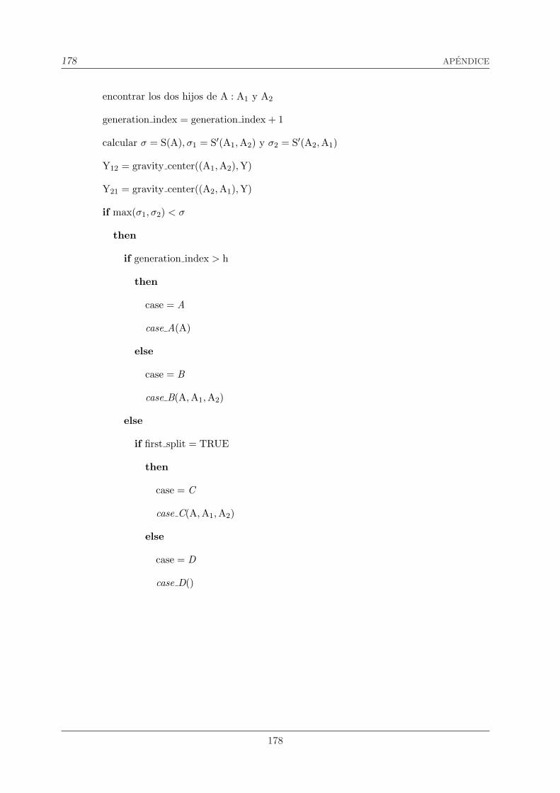
178 APENDICE
encontrar los dos hijos de A : A1 y A2
generation index = generation index + 1
calcular σ = S(A), σ1 = S′(A1,A2) y σ2 = S′(A2, A1)
Y12 = gravity center((A1, A2), Y)
Y21 = gravity center((A2, A1), Y)
if max(σ1, σ2) < σ
then
if generation index > h
then
case = A
case A(A)
else
case = B
case B(A, A1, A2)
else
if first split = TRUE
then
case = C
case C(A,A1, A2)
else
case = D
case D()
178
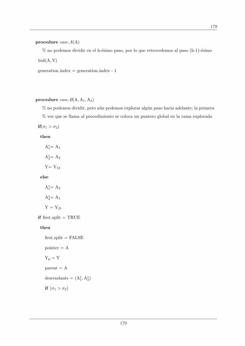
179
procedure case A(A)
% no podemos dividir en el h-esimo paso, por lo que retrocedemos al paso (h-1)-esimo
link(A,Y)
generation index = generation index - 1
procedure case B(A, A1,A2)
% no podemos dividir, pero aun podemos explorar algun paso hacia adelante; la primera
% vez que se llama al procedimiento se coloca un puntero global en la rama explorada
if(σ1 > σ2)
then
A∗1= A1
A∗2= A2
Y= Y12
else
A∗1= A2
A∗2= A1
Y = Y21
if first split = TRUE
then
first split = FALSE
pointer = A
Yp = Y
parent = A
descendants = (A∗1,A∗2)
if (σ1 > σ2)
179

180 APENDICE
then
Yd = Y12
else
Yd = Y21
if A∗1 y A∗2 son hojas
then
link(A, Yp)
else
g = generation index
link( (A∗1, A∗2), Y)
look ahead(A∗1, Y)
if pointer = parent
then
generation index = g
look ahead(A∗2, Y)
if pointer = parent
then
link(A, Y)
procedure case C (A, A1, A2)
% dividimos normalmente
generation index = 0
if (σ1 > σ2)
then
A∗1 = A1
180

181
A∗2 = A2
Y = Y12
else
A∗1 = A2
A∗2 = A1
Y = Y21
pointer = A∗1
link((A∗1, A∗2), Y)
look ahead(A∗1, Y)
pointer = A∗2
generation index = 0
first split = TRUE
look ahead(A∗2, Y)
procedure case D()
% dividimos la rama marcada con el puntero global
Y = Yd
link(descendants, Y)
pointer = descendants(1)
pointer2 = descendants(2)
generation index = 0
first split = TRUE
look ahead(pointer, Y)
generation index = 0
pointer = pointer2
181

182 APENDICE
first split = TRUE
look ahead(pointer, Y)
182

Referencias
Aczel, J. y Daroczy, Z. (1975). On measures of information and their generalizations. Academic
Press. New York.
Akaike, H. (1974). A new look at statistical model identification. IEEE Transactions on
Automatic Control, 19:716–723.
Al-Daoud, M. y Roberts, S. (1994). New methods for the initialization of clusters. Technical
report, 94.34.
Alon, U., Barkai, N., Notterman, D., Gish, K., Ybarra, S., Mack, D. y Levine, A. (1999). Broad
patterns of gene expression revealed by clustering analysis of tumour and colon tissues. Proc.
Natl. Acad. Sci., 96 (12):6745–6750.
Arabie, P. y Boorman, S. (1973). Multidimensional scaling of measures of distance between
partitions. Journal of Mathematical Psychology, 10:148–203.
Arcones, M. y Gine, E. (1992). Bootstrap of M–estimators and related statistical functionals.
Exploring the Limits of Bootstrap. Wiley. New York.
Bach, F. y Jordan, M. (2005). Blind one-microphone speech separation: a spectral learning
approach. Advances in Neural Information Processing Systems, 17.
Barron, A., Rissanen, J. y Yu, B. (1998). The minimum description length principle in coding
and modeling. IEEE Transactions on Information Theory, 44 (6):2743–2760.
183

184 REFERENCIAS
Bezdek, J. (1981). Pattern recognition with fuzzy objective function algorithms. Kluwer Acad-
emic Publishers. Norwell, MA, USA.
Bolstad, B., Irizarry, R., Astrand, M. y Speed, T. (2003). A comparison of normalization meth-
ods for high density oligonucleotide array data based on bias and variance. Bioinformatics,
19:185–193.
Bradley, P. y Fayyad, U. (1998). Refining initial points for k-means clustering. Proceedings of
the 15th International Conference of Machine Learning.
Brazma, A., Hingamp, P., Quackenbush, J., Sherlock, G., Spellman, P., Stoeckert, C., Aach,
J., Ansorge, W., Ball, C. y Causton, H. (2001). Minimum information about a microarray
experiment (miame) –towards standards for microarray data. Nature Genetics, 29:365–371.
Breckenridge, J. (1989). Replicating cluster analysis: method, consistency and validity. Multi-
variate Behavioral Research, 24 (2):147–161.
Breiman, L. (1996). Bagging predictors. Machine Learning, 24(2):123–140.
Brown, G. y Cooke, M. (1994). Computational auditory scene analysis. Computer Speech and
Language, 8:297–333.
Butte, A. y Kohane, I. (2000). Mutual information relevance networks: functional genomic
clustering using pairwise entropy measurements. Pacific Symposium on Biocomputing.
Calinski, R. y Harabasz, J. (1974). A dendrite method for cluster analysis. Communications
in Statistics, 3:1–27.
Causton, H., Quackenbush, J. y Brazma, A. (2003). Microarray gene expression data analysis:
a beginner’s guide. Blackwell Publishers.
Charikar, M. y Panigrahy, R. (2004). Clustering to minimize the sum of cluster diameters.
Journal of Computer and System Sciences, 68 (2):417–441.
184

REFERENCIAS 185
Chen, D., Toone, W., Mata, J., Lyne, R., Burns, G., Kivinen, K., Brazma, A., Jones, N. y
Bahler, J. (2003). Global transcriptional responses of fission yeast to enviromental stress.
Molecular Biology of the Cell, 14:214–229.
Cheng, C. y Li, L. (2005). Sub-array normalization subject to differentiation. Nucleic Acids
Res., 33 (7):5565–5573.
Cho, R., Campbell, M., Winzeler, E., Steinmetz, L., Conway, A., Wodicka, L., Wolfsberg, T.,
Gabrielian, A., Landsman, D., Lockhart, D. y Davis, R. (1998). A genome-wide transcrip-
tional analysis of the mitotic cell cycle. Molecular Cell, 2:65–73.
Chu, S., DeRisi, J., Eisen, M., Mulholland, J., Botstein, D., Brown, P. y Futcher, B. (1998).
The transcriptional program of sporulation in budding yeast. Science, 282:699–705.
Clatworthy, J., Buick, D., Hankins, M., Weinman, J. y Horne, R. (2005). The use and reporting
of cluster analysis in health psychology: A review. British Journal of Health Psychology,
10:329–358.
de Berg, M., Schwarzkopf, O., van Kreveld, M. y Overmars, M. (2000). Computational geom-
etry: algorithms and applications. Springer-Verlag.
DeRisi, J., Iyer, V. y Brown, P. (1997). Exploring the metabolic and genetic control of gene
expression on a genomic scale. Science, 278:680–686.
Doddi, S., Marathe, M., Ravi, S., Taylor, D. y Widmayer, P. (2000). Approximation algorithms
for clustering to minimize the sum of diameters. Nordic Journal of Computing, 7 (3):185–203.
Donoho, D. y Gasko, M. (1992). Breakdown properties of location estimates based on halfspace
depth and projected outlyingness. Annals of Statistics, 20:1803–1827.
Dopazo, J. y Carazo, J. (1997). Phylogenetic reconstruction using a growing neural network
that adopts the topology of a phylogenetic tree. Journal of Molecular Evolution, 44:226–233.
185

186 REFERENCIAS
Du, Q., Faber, V. y Gunzburger, M. (1999). Centroidal voronoi tesselations: applications and
algorithms. SIAM Rev., 41:637–676.
Dudoit, S. y Fridlyand, J. (2002). A prediction-based resampling method for estimating the
number of clusters in a dataset. Genome Biology, 3 (7):1–21.
Dudoit, S. y Fridlyand, J. (2003). Bagging to improve the accuracy of a clustering procedure.
Bioinformatics, 19 (9):1090–1099.
Eades, P., McKay, B. y Wormald, N. (1986). On an edge crossing problem.
Eisen, M., Spellman, P., Brown, P. y Botstein, D. (1998). Cluster analysis and display of
genome-wide expression patterns. Proc. Natl. Acad. Sci., 95 (25):14863–14868.
Everitt, B. (1980). Cluster Analysis. John Wiley and Sons. Halsted Press, New York.
Forbes, A. (1995). Classification-algorithm evaluation – 5 performance-measures based on
confusion matrices. J. Clin. Monit., 11:159–164.
Forgy, E. (1965). Cluster analysis of multivariate data: efficiency vs interpretability of classifi-
cations. Biometrics, 21:768.
Fowlkes, E. y Mallows, C. (1983). A method for comparing two hierarchical clusterings. Journal
of the American Statistical Association, 78:553–584.
Futschik, M. y Kasabov, N. (2002). Fuzzy clustering of gene expression data. Proceedings of
World Congress of Computational Intelligence, WCCI.
Gansner, E., Koutsofios, E., North, S. y Vo, K. (1993). A technique for drawing directed graphs.
IEEE Trans. on Software Engineering, 19 (3):214–230.
Garey, M. y Johnson, D. (1979). Computers and intractability: a guide to the theory of NP-
completeness. W.H.Freeman.
186

REFERENCIAS 187
Garey, M. y Johnson, D. (1983). Crossing number is np-complete. SIAM J.Algebraic Discrete
Methods, 4:312–316.
Garey, M., Johnson, D. y Witsenhausen, H. (1982). The complexity of the generalized lloyd-max
problem. IEEE Transactions on Information Theory, 28 (2):255–256.
Gasch, A. y Eisen, M. (2002). Exploring the conditional coregulation of yeast gene expression
through fuzzy k-means clustering. Genome Biology, 3 (11):1–22.
Golub, T., Slonim, D., Tamayo, P., Huard, C., Gaasenbeek, M., Mesirov, J., Coller, H., Loh,
M., Downing, J., Caligiuri, M., Bloomfield, C. y Lander, E. (1999). Molecular classification of
cancer: class discovery and class prediction by gene expression monitoring. Science, 286:531–
537.
Gordon, A. (1999). Classification. Chapman and Hall. CRC press, London.
Gross, J. y Yellen, J. (1999). Graph theory and its applications. CRC Press.
Grotkjaer, T., Winther, O., Regenberg, B., Nielsen, J. y Hansen, L. (2006). Robust multi-scale
clustering of large dna microarray datasets with the consensus algorithm. Bioinformatics,
22:58–67.
Gusfield, D. (2002). Partition-distance: a problem and class of perfect graphs arising in clus-
tering. Information Processing Letters, 82 (3):159–164.
Hansen, M. y Yu, B. (2001). Model selection and the principle of the minimum description
length. Journal of the American Statistical Association, 96 (454):746–774.
Harper, D. (1999). Numerical Palaeobiology. John Wiley and Sons.
Hart, C., Sharenbroich, L., Bornstein, B., Trout, D., King, B., Mjolsness, E. y Wold, B. (2005).
A mathematical and computational framework for quantitative comparison and integration
of large-scale gene expression data. Nucleic Acids Res., 33 (8):2580–2594.
187

188 REFERENCIAS
Hartigan, J. (1975). Clustering Algorithms. John Wiley and Sons. New York.
Hartuv, E., Schmitt, A., Lange, J., Meier-Ewert, S., Lehrach, H. y Shamir, R. (1999). An
algorithm for clustering cdnas for gene expression analysis using short oligonucleotide finger-
prints. Proceedings 3rd International Symposium on Computational Molecular Biology.
He, J., Lan, M., Tan, C., Sung, S. y Low, H. (2004). Initialization of cluster refinement algo-
rithms: a review and comparative study. International Joint Conference on Neural Networks.
Herrero, J., Valencia, A. y Dopazo, J. (2001). A hierarchical unsupervised growing neural
network for clustering gene expression patterns. Bioinformatics, 17:126–136.
Heyer, L., Kruglyak, S. y Yooseph, S. (1999). Exploring expression data: identification and
analysis of coexpressed genes. Genome Research, 9 (11):1106–1115.
Hoff, K., Culver, T., Keyser, J., Lin, M. y Manocha, D. (1999). Fast computation of generalized
voronoi diagrams using graphics hardware. Computer Graphics, 33:277–286.
Hubert, L. y Arabie, P. (1985). Comparing partitions. Journal of Classification, 2:193–198.
Jonnalagadda, S. y Srinivasan, R. (2004). An information theory approach for validating
clusters in microarray data. ISMB.
Jornsten, R. (2004). Clustering and classification based on the l1-data depth. Journal of
Multivariate Analysis, 90(1):67–89.
Jornsten, R., Vardi, Y. y Zhang, C. (2002). A Robust Clustering Method and Visualization
Tool Based on Data Depth. Y.Dodge.
Jornsten, R. y Yu, B. (2003). Simultaneous gene clustering and subset selection for sample
classification via mdl. Bioinformatics, 19 (9):1100–1109.
188

REFERENCIAS 189
Kapushesky, M., Kemmeren, P., Culhane, A., Durinck, S., Ihmels, J., Korner, C., Kull, M.,
Torrente, A., Sarkans, U., Vilo, J. y Brazma, A. (2004). Expression profiler: next generation–
an online platform for analysis of microarray data. Nucleic Acids Res., 32:W465–W470.
Katsavounidis, I., Kuo, C. y Zhang, Z. (1994). A new initialization technique for generalized
lloyd iteration. IEEE Signal Processing Letters, 1 (10):144–146.
Kaufman, L. y Rousseeuw, P. (1990). Finding groups in data: an introduction to cluster analysis.
Wiley. New York.
Kohonen, T. (1990). The self-organizing map. Proceedings of the IEEE, 9:1464–1479.
Kolmogorov, A. (1965). Three approaches to the quantitative definition of information. Prob-
lems Inform. Transmission, 1 (1):1–7.
Krzanowski, W. y Lai, Y. (1985). A criterion for determining the number of groups in a data
set using sum of squares clustering. Biometrics, 44:23–34.
Laszlo, M. y Mukherjee, S. (2006). A genetic algorithm using hyper-quadtrees for low-
dimensional k -means clustering. IEEE Transactions on Pattern Analysis and Machine In-
telligence, 8.
Leisch, F. (1999). Bagged clustering. Technical report, 51.
Li, M. y Vitanyi, P. (1997). An introduction to Kolmogorov complexity and its applications.
Springer-Verlag. New York.
Liu, R. (1990). On a notion of data depth based on random simplices. Annals of Statistics,
18:405–414.
Lopez-Pintado, S. y Romo, J. (2006). On the concept of depth for functional data. Technical
report, 06-30, Statistics and Econometrics Series 12, Department of Statistics, Universidad
Carlos III de Madrid.
189

190 REFERENCIAS
MacQueen, J. (1967). Some methods for classification and analysis of multivariate observations.
Proceedings of the 5th Berkeley simposium in mathematics and probability.
Meila, M. y Shi, J. (2001). Learning segmentation with random walk. Neural Information
Processing Systems.
Michaels, G., Carr, D., Askenazi, M., Fuhram, S., Wen, X. y Somoggi, R. (1998). Cluster
analysis and data visualization of large-scale gene expression data. Pacific Symposium on
Biocomputing, 3:42–53.
Milligan, G. y Cooper, M. (1985). An examination of procedures for determining the number
of clusters in a data set. Psychometrika, 50(2):159–179.
Monma, C. y Suri, S. (1991). Partitioning points and graphs to minimize the maximum or
the sum of diameters. Proceedings of the 6th International Conf. Theory Appl. Graphs,
2:899–912.
Oja, H. (1983). Descriptive statistics for multivariate distributions. Statistics and Probability
Letters, 1:327–332.
Pena, D., Rodrıguez, J. y Tiao, G. (2004). A general partition cluster algorithm. COMPSTAT.
Proceedings in computational statistics, 371–380.
Pedrycz, W. (2005). Knowledge-based clustering. From data to information granules. Wiley.
Pentney, W. y Meila, M. (2005). Spectral clustering of biological sequence data. Proceedings
of the 25th Anual Conference of AAAI.
Pollard, D. (1982). A central limit theorem for k-means clustering. Annals of Probability,
10:919–926.
Quackenbush, J. (2001). Computational analysis of microarray data. Nature Reviews Genetics,
2:418–427.
190

REFERENCIAS 191
Radonjic, M., Andrau, J., Lijnzaad, P., Kemmeren, P., Kockelkorn, T., van Leenen, D., van
Berkum, N. y Holstege, F. (2005). Genome-wide analyses reveal rna polymerase ii located up-
stream of genes poised for rapid response upon s. cerevisiae stationary phase exit. Molecular
Cell, 18:171–183.
Rand, W. (1971). Objective criteria for the evaluation of clustering methods. Journal of the
American Statistical Association, 66:846–850.
Ripley, B. y Hjort, N. (1996). Pattern Recognition and Neural Networks. Cambridge University
Press.
Rissanen, J. (1978). Modelling by shortest data description. Automatica, 14:465–471.
Sanguinetti, G., Laidler, J. y Lawrence, N. (2005). Automatic determination of the num-
ber of clusters using spectral algorithms. IEEE Workshop on Machine Learning for Signal
Processing, 55–60.
Sedgewick, R. (1986). A new upper bound for shell sort. J.Algorithms, 7:159–173.
Shannon, C. (1948). A mathematical theory of communication. 27:379–423, 623–656.
Sharan, R. y Shamir, R. (2000). Click: A clustering algorithm with applications to gene ex-
pression data. ISMB.
Shi, J. y Malik, J. (2000). Normalized cuts and image segmentation. IEEE Transactions on
Pattern Analysis and Machine Intelligence, 22.
Shokoufandeh, A., Mancoridis, S., Denton, T. y Maycock, M. (2005). Spectral and meta-
heuristic algorithms for software clustering. Journal of Systems and Software, 77:213–223.
Shokoufandeh, A., Mancoridis, S. y Maycock, M. (2002). Applying spectral methods to soft-
ware clustering. Proceedings of the Ninth Working Conference on Reverse Engineereing
(WCRE02).
191

192 REFERENCIAS
Somolonoff, R. (1964). A formal theory of inductive inference. Information and Control, 7:1–
22,224–254.
Sugar, C. (1998). Techniques for clustering and classification with applications to medical
problems. PhD Thesis.
Sugar, C. y James, G. (2003). Finding the number of clusters in a data set: an information
theoretic approach. Journal of the American Statistical Association, 98:750–763.
Swets, J. (1988). Measuring the accuracy of diagnostic systems. Science, 240:1285–1293.
Tamayo, P., Slonim, D., Mesirov, J., Zhu, Q., Kitareewan, S., Dmitrovsky, E., Lander, E. y
Golub, T. (1999). Interpreting patterns of gene expression with self-organizing maps: methods
and application to hematopoetic differentiation. Proc. Natl. Acad. Sci., 96:2907–2912.
Tavazoie, S., Hughes, D., Campbell, M., Cho, R. y Church, G. (1999). Systematic determination
of genetic network architecture. Nature Genetics, 22:281–285.
Tibshirani, R., Hastie, T., Eisen, M., Ross, D., Botstein, D. y Brown, P. (1999). Clustering
methods for the analysis of dna microarray data. Technical report.
Tibshirani, R., Walther, G. y Hastie, T. (2001). Estimating the number of data clusters via
the gap statistic. J.R.Statist.Soc.B, 63:411–423.
Toronen, P., Kolehmainen, M., Wong, G. y Castren, E. (1999). Analysis of gene expression
data using self-organizing maps. FEBS Lett, 451:142–146.
Tou, J. y Gonzalez, R. (1974). Pattern Recognition Principles. Addison–Wesley.
Tukey, J. (1975). Mathematics and the picturing of data. Proceedings of the International
Congress of Mathematicians.
Vardi, Y. y Zhang, C. (2000). The multivariate l1-median and associated data depth. Proc.
Natl. Acad. Sci., 97:1423–1426.
192

REFERENCIAS 193
Verma, D. y Meila, M. (University of Washington, 2003). A comparison of spectral clustering
algorithms. Technical report.
Vilo, J., Brazma, A., Jonassen, I., Robinson, A. y Ukkonen, E. (2000). Mining for putative
regulatory elements in the yeast genome using gene expression data. ISMB.
Weber, A. (1929). Theory of location of industries [English translation by C.J.Friedrich from
Weber’s 1909 book]. Univ. Chicago Press.
Wen, X., Fuhrman, S., Michaels, G., Carr, D., Smith, S., Barker, J. y Somogyi, R. (1998).
Large-scale temporal gene expression mapping of central nervous system development. Proc.
Natl. Acad. Sci., 95:334–339.
Yeh, A. y Singh, K. (1997). Balanced confidence regions based on Tukey’s depth and the
bootstrap. J.R.Statist.Soc.B, 59:639–652.
193