Ralph  Cueva  Partners:  Michael  Bunger  and  Pavel  Aprelev  Physics  121H    May  24,  2010  

Circulating Charged Particles in a Magnetic Field  Abstract  

The  purpose  of  the  experiment  was  to  determine  the  ratio  of  the  electron’s  

charge  to  its  mass .  We  used  the    apparatus  to  measure  the  radius  of  an  electron  

beam.  Our  value  for    is .  When  we  compare  the  

experimental  value  to  the  actual  value, ,  we  calculated  a  11.1%  error.  

The  experimental  value  did  not  fall  within  the  uncertainties.  Introduction/Theory  

     

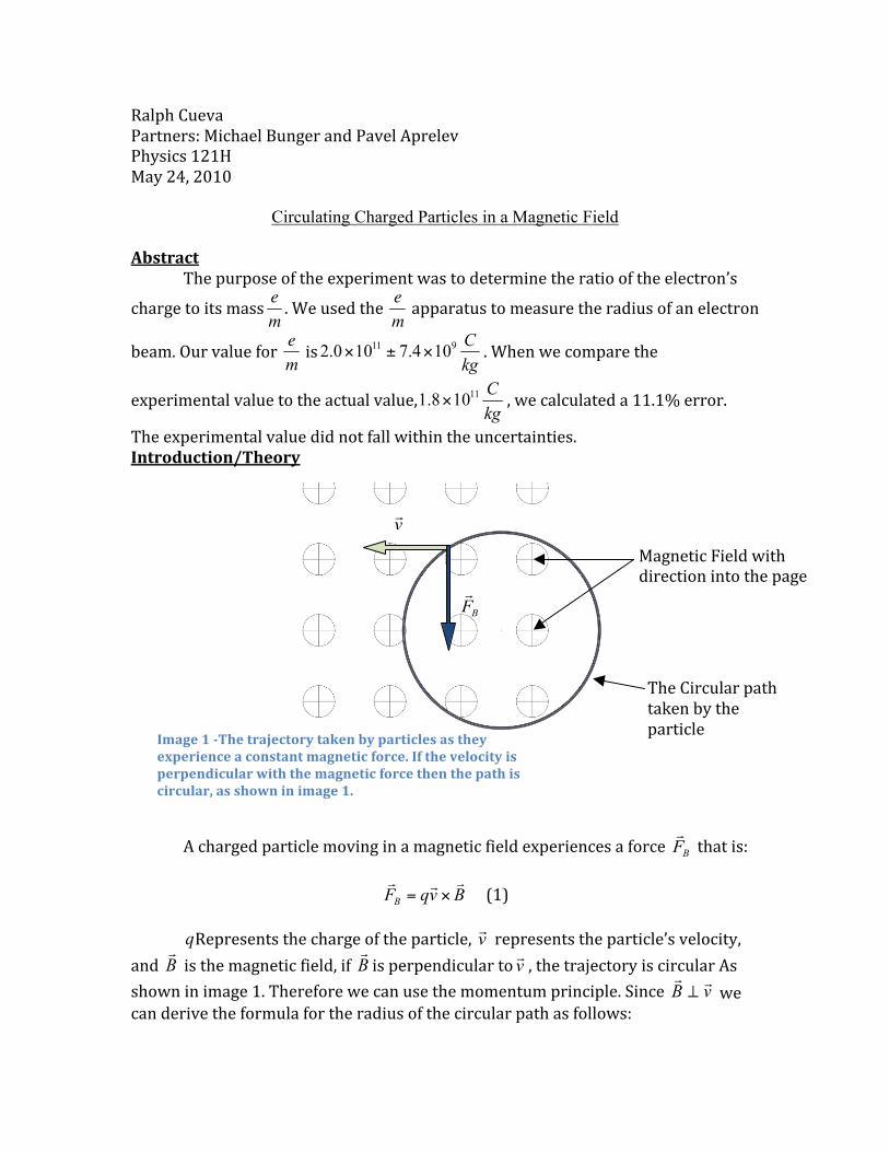
                           A  charged  particle  moving  in  a  magnetic  field  experiences  a  force    that  is:  

    (1)  

 Represents  the  charge  of  the  particle,    represents  the  particle’s  velocity,  

and    is  the  magnetic  field,  if   is  perpendicular  to ,  the  trajectory  is  circular  As  shown  in  image  1.  Therefore  we  can  use  the  momentum  principle.  Since    we  can  derive  the  formula  for  the  radius  of  the  circular  path  as  follows:  

 

Image  1  -­The  trajectory  taken  by  particles  as  they  experience  a  constant  magnetic  force.  If  the  velocity  is  perpendicular  with  the  magnetic  force  then  the  path  is  circular,  as  shown  in  image  1.  

 

 

Magnetic  Field  with  direction  into  the  page  

The  Circular  path  taken  by  the  particle  

 

   

   

 The  magnitude  of  the  magnetic  force  is  given  by ,  this  is  then  equal  to  the  

magnitude  of  the  change  of  momentum .  Since  we  know  the  motion  is  circular,  

the  magnitude  of  change  in  momentum  equals  (centripetal  force)  which  then  equals  to  the  magnetic  force  given  in  formula  (1).  The  angle  is    because .  If   <<c  then  gamma ,  then  we  can  solve  for  R  as  follows:  

 

  (2)  

 Where    is  the  mass  of  the  charged  particle  and  the  charge  of  an  electron  is  

e.  If  an  electron,  initially  at  rest,  is  accelerated  through  an  electric  potential  difference ,  then  its  kinetic  energy  is  equal  to  the  change  of  the  potential  energy:  

 and  because  energy  is  conserved  we  know  that:    

(3)  

 From  equations  (2)  and  (3)  we  can  eliminate ,  and  substituting  the  

magnitude  of  the  electron  charge  e  for ,  we  obtain  the  following:    

(4)  

 and  solve  for    as  follows:      

 (5)  

 

Formula  (5)  is  key  to  our  experiment.  This  is  the  equation  that  we  used  to  

calculate  the    ratio.  We  know  that  the  slope  is   for  the  function  of .  The  

slope  of  this  line  equals  the    ratio.  

To  calculate  the   ratio  we  need  to  know  the  potential    that  accelerates  

the  electrons,  the  magnitude  of  the  magnetic  field    and  the  radius  of  the  circular  

path  of  the  electron  beam .  The  magnetic  field  of  the  Helmholtz  coils  can  be  found  using  the  following:  

 

(6)  

 where  the  number  of  turns  of  the  wire  in  the  coil  is   ,  constant  

,  the  current  in  the  coils  is   ,  and  the  coil’s  radius  is   .  

   Procedure  

   

   Figure  

1  -­‐shows  our  basic  setup.  We  included  Multimeters  in  order  to  read  an  accurate  current  and  accurate  acclerating  voltage.  The  Helmholtz  coils  create  the  magnetic  field  that  allowed  for  the  circular  path.  The  vaccumed  bulb  had  the  

Figure  1-­  the  e/m  apparatus  and  power  supplies  

Helmholtz  Coils  

 Vacuumed  Bulb    

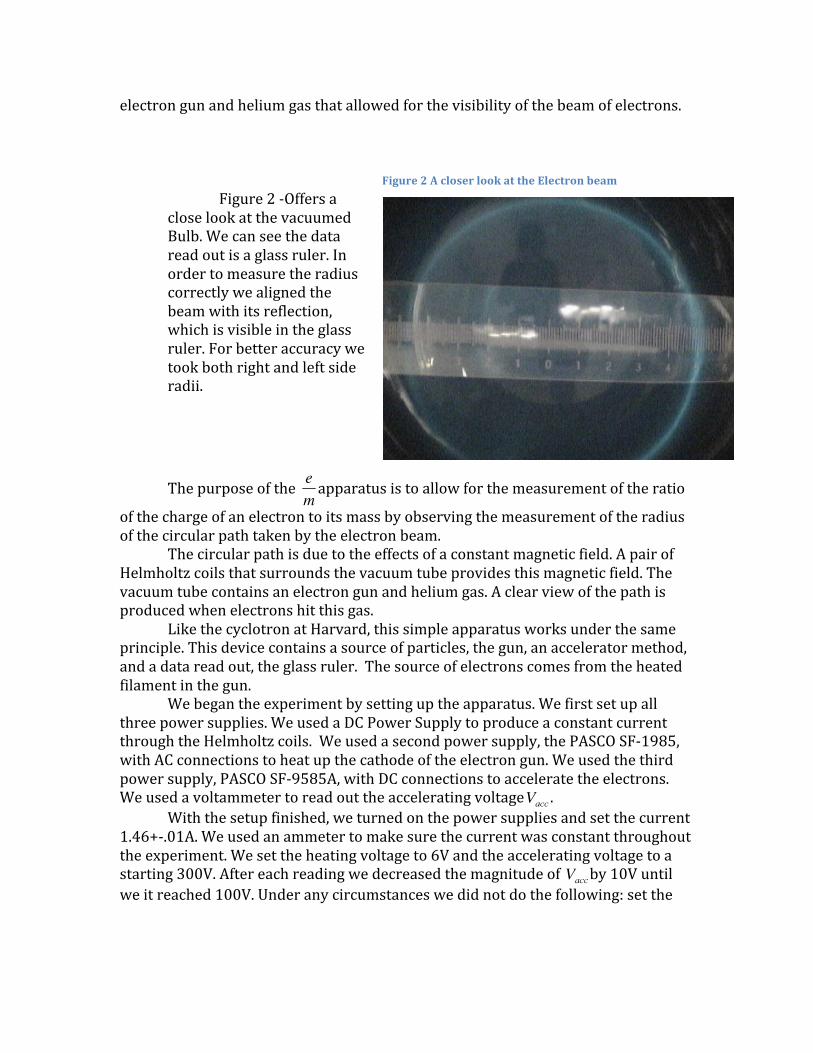
electron  gun  and  helium  gas  that  allowed  for  the  visibility  of  the  beam  of  electrons.    

     

 Figure  2  -­‐Offers  a  close  look  at  the  vacuumed  Bulb.  We  can  see  the  data  read  out  is  a  glass  ruler.  In  order  to  measure  the  radius  correctly  we  aligned  the  beam  with  its  reflection,  which  is  visible  in  the  glass  ruler.  For  better  accuracy  we  took  both  right  and  left  side  radii.  

     

 

The  purpose  of  the   apparatus  is  to  allow  for  the  measurement  of  the  ratio  

of  the  charge  of  an  electron  to  its  mass  by  observing  the  measurement  of  the  radius  of  the  circular  path  taken  by  the  electron  beam.  

The  circular  path  is  due  to  the  effects  of  a  constant  magnetic  field.  A  pair  of  Helmholtz  coils  that  surrounds  the  vacuum  tube  provides  this  magnetic  field.  The  vacuum  tube  contains  an  electron  gun  and  helium  gas.  A  clear  view  of  the  path  is  produced  when  electrons  hit  this  gas.     Like  the  cyclotron  at  Harvard,  this  simple  apparatus  works  under  the  same  principle.  This  device  contains  a  source  of  particles,  the  gun,  an  accelerator  method,  and  a  data  read  out,  the  glass  ruler.    The  source  of  electrons  comes  from  the  heated  filament  in  the  gun.    

We  began  the  experiment  by  setting  up  the  apparatus.  We  first  set  up  all  three  power  supplies.  We  used  a  DC  Power  Supply  to  produce  a  constant  current  through  the  Helmholtz  coils.    We  used  a  second  power  supply,  the  PASCO  SF-­‐1985,  with  AC  connections  to  heat  up  the  cathode  of  the  electron  gun.  We  used  the  third  power  supply,  PASCO  SF-­‐9585A,  with  DC  connections  to  accelerate  the  electrons.  We  used  a  voltammeter  to  read  out  the  accelerating  voltage .    

With  the  setup  finished,  we  turned  on  the  power  supplies  and  set  the  current  1.46+-­‐.01A.  We  used  an  ammeter  to  make  sure  the  current  was  constant  throughout  the  experiment.  We  set  the  heating  voltage  to  6V  and  the  accelerating  voltage  to  a  starting  300V.  After  each  reading  we  decreased  the  magnitude  of   by  10V  until  we  it  reached  100V.  Under  any  circumstances  we  did  not  do  the  following:  set  the  

Figure  2  A  closer  look  at  the  Electron  beam    

amperage  to  anything  higher  than  2A,  or  set  the  Voltage  to  anything  over  6.3V,  if  this  

is  done  the  filament  of  the  gun  will  burn  out,  thus  destroying  the   apparatus.  

After  the  electron  beam  was  clear  we  started  recording  data.  By  using  the  glass  ruler  in  the  apparatus  we  recorded  the  left  and  right  radii  of  the  circular  path.  Two  of  us  gave  readings  while  one  of  us  recorded  the  data  in  an  excel  file.   Data/Analysis The data shown below is the left and right radius of the electron beam at various Voltages. Our data shows that the data readout method, the glass ruler is efficient. The difference in both read outs was small.

Radius of the electron Beam

  R(left)   R(right)   R(left)   R(right)   R(avg)    300   4.8   5   4.8   5.1   0.04925   0.002426  

290   4.8   4.9   4.7   4.9   0.04825   0.002328  

279   4.7   4.9   4.7   4.9   0.048   0.002304  

270   4.6   4.8   4.6   4.8   0.047   0.002209  

259   4.5   4.8   4.5   4.7   0.04625   0.002139  

250   4.5   4.7   4.5   4.6   0.04575   0.002093  

239   4.4   4.5   4.4   4.5   0.0445   0.00198  

231   4.3   4.5   4.3   4.5   0.044   0.001936  

221   4.2   4.4   4.2   4.4   0.043   0.001849  

210   4   4.2   4.1   4.3   0.0415   0.001722  

200   3.9   4.2   4   4.2   0.04075   0.001661  

191   3.8   4.1   3.8   4.1   0.0395   0.00156  

181   3.7   4   3.8   4.1   0.039   0.001521  

171   3.6   3.9   3.6   4   0.03775   0.001425  

160   3.5   3.8   3.5   3.8   0.0365   0.001332  

150   3.3   3.7   3.4   3.8   0.0355   0.00126  

140   3.2   3.6   3.2   3.5   0.03375   0.001139  

131   3   3.5   3.1   3.4   0.0325   0.001056  

120   3   3.3   3   3.3   0.0315   0.000992  

111   2.9   3.2   2.8   3.1   0.03   0.0009  

101   2.6   3   2.6   3   0.028   0.000784  Data  table  1  shows  the  left  and  right  radius  dependence  in  the  accelerating  voltage  

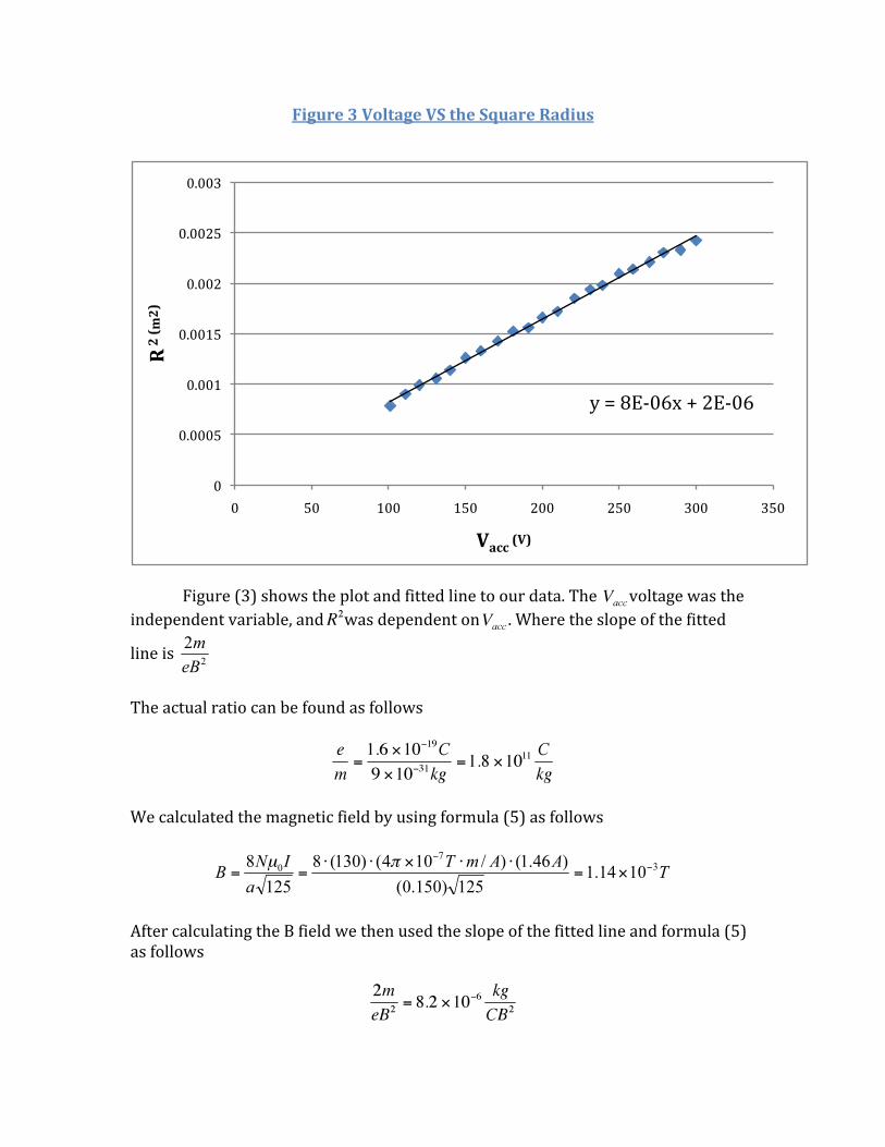
Figure  3  Voltage  VS  the  Square  Radius  

   

Figure  (3)  shows  the  plot  and  fitted  line  to  our  data.  The   voltage  was  the  independent  variable,  and was  dependent  on .  Where  the  slope  of  the  fitted  

line  is    

 The  actual  ratio  can  be  found  as  follows    

 

 We  calculated  the  magnetic  field  by  using  formula  (5)  as  follows    

 

 After  calculating  the  B  field  we  then  used  the  slope  of  the  fitted  line  and  formula  (5)  as  follows    

 

 

y  =  8E-­‐06x  +  2E-­‐06  

0  

0.0005  

0.001  

0.0015  

0.002  

0.0025  

0.003  

0   50   100   150   200   250   300   350  

R  2  (m2)  

Vacc  (V)  

   By  solving  for  m/e  we  got    

 

 By  dividing  our  answer  1  we  got  the  ratio  as  follows    

 

Uncertainties  for  all  measured  Quantities  Our  measured  Quantities  are  the  magnetic  field  of  the  Helmholtz  Coils,  the  

Current  running  thought  the  coils,  the  slope  of  the  fitted  line  (this  will  include  the  uncertainties  of  the  radiuses    recorded  and  the  accelerating  voltages   ,  and  the  

ratio  of   .  

We  calculated  the  uncertainty  for  the  magnetic  field  as  follows:    

 

Our  final  result  for  the  magnetic  field  is    The  uncertainty  of  the  current  comes  from  the  accuracy  of  the  ammeter,  which  is  1%  thus    

 Our  result  for  the  current  is      We  used  excels  regression  to  find  the  uncertainty  for  the  radiuses  and  the  accelerating  voltage  as  follows  

Uncertainty  for  the  slope=  

Our  result  for  the  slope  of  the  line  is    

Finally,  we  used  the  uncertainties  to  calculate  the  uncertainty  of  the  ratio  as  follows  

   

Our  result  for  the    ratio  is    

 Comparison  of  experimental  value  with  actual  value  

 We  used  the  following  equation  to  find  the  percent  difference  of  the  experimental  ratio  to  the  actual  ratio    

 

     Discussion/Conclusion  

  The  experiment’s  purpose  was  to  determine  the  ratio  of  the  electron’s  

charge  to  its  mass .  We  used  the    apparatus  to  measure  the  radius  of  an  electron  

beam  that  had  a  circular  path.  This  path  was  a  direct  effect  of  the  magnetic  force  the  Helmholtz  coils  have  on  the  electrons.  The  magnetic  field  of  the  Helmholtz  coils  was  so  large  (two  order  of  magnitude  larger  than  the  earth’s  magnetic  field)  that  we  did  

not  take  into  account  earth’s  magnetic  field.  Our  value  for    is

.  When  we  compared  the  experimental  value  to  the  actual  

value,  we  got  an  11.1%  error.  The  experimental  value  did  not  fall  within  

the  uncertainties.  The  error  most  likely  occurred  in  the  read  out  the  left  and  right  radii.  Better  accuracy  in  our  readings  for  the  accelerating  voltage,  current  in  the  coils,  and  radius  of  the  circular  path  can  solve  the  problem.          References  http://www.physics.harvard.edu/~wilson/cyclotron/history.html