Testing and Estimation of Models with Stochastic Trends

Fabio Busetti

The London School of Economics and Political Science

A thesis submitted for the PhD degree, University of London.

December 2000

1

UMI Number: U615204

All rights reserved

INFORMATION TO ALL USERS The quality of this reproduction is dependent upon the quality of the copy submitted.

In the unlikely event that the author did not send a complete manuscript and there are missing pages, these will be noted. Also, if material had to be removed,

a note will indicate the deletion.

Dissertation Publishing

UMI U615204Published by ProQuest LLC 2014. Copyright in the Dissertation held by the Author.

Microform Edition © ProQuest LLC.All rights reserved. This work is protected against

unauthorized copying under Title 17, United States Code.

ProQuest LLC 789 East Eisenhower Parkway

P.O. Box 1346 Ann Arbor, Ml 48106-1346

I M c L Z S

F7 8

7 5 ) 3 3 7

Abstract

The thesis considers time series and econometric models with stochastic trend

components. Locally Best Invariant tests for the presence of stochastic trends

are constructed and their asymptotic distributions derived. Particular attention is paid to models with structural breaks, as the tests have high power also against

alternative hypotheses in which the trends of the series contain a small number

of breaks but are otherwise deterministic. Asymptotic critical values of the tests

are tabulated for series with a single breakpoint. A modification of the LBI

statistic is then proposed, for which the asymptotic distribution depends only

on the number of the breaks and not on their location.

Common stochastic trends imply cointegration and thus testing the number

of common trends can also be regarded as testing the dimension of the cointe­

gration space. A test for common trends recently proposed in the literature is

extended to series which contain structural breaks.

Testing for the presence of a nonstationary seasonal component is then exam­

ined. The LBI test, adjusted for serial correlation by means of a nonparametric correction, is extended in various directions and its performance is compared

with that of a parametric test.

Representation, estimation and tests of cointegrated structural time series

models form the subject of one chapter, where numerous links with the literature

on vector autoregressions are established.

Panel data regression models where the individual effects take the form of

individual specific random walks are considered in the last chapter. Imposing

the constraint of a common signal-to-noise ratio across individuals makes the

maximum likelihood estimator computationally feasible also when the number

of units in the cross section is large. For these models an average LBI test for

stationarity and for the presence of fixed effects is proposed.

2

Acknowledgements

I wish to express my gratitude to Professor Andrew Harvey for his guidance,

encouragement and constructive criticism during the course of this research. I

am greatly indebted to him for sharing his views on the whole subject of time

series.

I have also benefited from the comments of several people in the Economics

Department of the LSE. I would like to specially thank Professor Peter Robinson,

Dr. Javier Hidalgo, Liudas Giraitis and my office mate Javier Hualde for the

valuable discussions on the issues raised in this work.

Finally I am mostly grateful to my family for their love and encouragement

throughout the years.Financial support from the Italian National Research Council (CNR) and

from the LSE is gratefully acknowledged.

3

Contents

1 Introduction 7

2 Preliminary concepts: the LBI test, state-space models, the Kalman filter 102.1 The LBI test ................................................................................... 11

2.1.1 Locally most powerful t e s t s .............................................. 112.1.2 Invariant te s ts ....................................................................... 132.1.3 LBI tests on the error covariance matrix in the linear re­

gression model .................................................................... 152.2 State space models and the Kalman filte r..................................... 182.3 GLS estimation using the Kalman filte r ........................................ 20

2.4 An Ox program for computing the maximum likelihood estimatorof a regression model with local level errors.................................. 22

3 Testing for a stochastic trend in univariate time series 263.1 The LBI test for a random walk co m p o n en t................................ 273.2 Testing in the presence of structural breaks................................ 31

3.3 A modified t e s t ................................................................................ 36

3.4 Unknown b reakpo in t...................................................................... 40

3.5 The treatment of serial correlation................................................. 423.5.1 Nonparametric correction ................................................. 433.5.2 Parametric correction........................................................... 44

3.6 Extensions......................................................................................... 463.7 Empirical exam ples......................................................................... 47

4

3.8 Proofs of this chapter’s propositions 51

4 Testing for (common) stochastic trends in multivariate tim e se­ries 574.1 LBI tests on the error covariance matrix in multivariate regression

m odels................................................................................................ 584.2 The distribution of the test for stochastic tre n d s ........................ 604.3 Testing in the presence of structural breaks.................................. 64

4.3.1 A modified sta tistic .............................................................. 68

4.4 Testing for common tren d s ............................................................. 694.5 Seasonal effects and weakly dependent exogenous regressors . . 714.6 E x am p les ......................................................................................... 734.7 Proofs of this chapter’s propositions.............................................. 78

5 Testing for stochastic seasonality 845.1 The Canova-Hansen t e s t ................................................................ 855.2 Deterministic trends, trend-breaks and integrated regressors . . 905.3 Deterministic breaks in the seasonal p a t t e r n .............................. 935.4 Parametric tests based on structural time series m odels............ 945.5 Example: UK m arriag es ................................................................ 975.6 Tests on groups of seasons............................................................. 1005.7 Example: Italian industrial p roduction ........................................ 1015.8 Seasonal unit root te s ts ................................................................... 102

5.9 Test of Seasonality ......................................................................... 1045.10 Testing for the presence of trading day e f fe c ts ........................... 1055.11 Concluding rem arks......................................................................... 107

6 Cointegration in structural tim e series models 1086.1 Cointegration and the Granger representation th e o re m ........... 1096.2 Representation of cointegrated structural time series................. 112

6.2.1 Common trends and cointegration..................................... 1136.2.2 Identification of the cointegrating vectors......................... 1146.2.3 VAR representation.............................................................. 115

5

6.2.4 Computing the VAR coefficients................................... 1176.3 Estimation and t e s t .................................................................... 1176.4 An example of cointegrated structural time series model . . . . 120

7 Estimation and tests of certain dynamic panel data models 1287.1 Introduction................................................................................ 1287.2 The baseline m o d e l.................................................................... 1307.3 Estimation of the m o d e l ........................................................... 1327.4 Testing exogeneity of the regressors........................................ 1377.5 Estimation with few time p e r io d s ............................................ 1397.6 Inclusion of a common trend com p onen t............................... 1397.7 Testing stationarity and fixed effects ........................................... 143

7.7.1 The distribution of the test statistic for stationarity . . . 1457.7.2 The distribution of the test statistic for fixed effects . . . 1457.7.3 Consistency of the t e s t .................................................. 148

7.8 Illustration: estimating a production function from a panel of USmanufacturing firms ....................................................................... 149

6

Chapter 1

Introduction

Economic theory often predicts that certain series, or some linear combination of them, ought to be stationary as opposed to having a stochastic trend com­ponent. Knowing the order of integration of a series is also a central issue in applied macroeconomics, when the objective is to identify a suitable econometric specification of aggregate behavioural relationships.

The literature has provided numerous statistical procedures to test the null hypothesis of unit root against the alternative of stationarity, starting with the seminal paper by Dickey and Fuller (1979). Less work has been devoted to developing tests where the null hypothesis is stationarity around a deterministic trend; important contributions in this direction are the articles by Nyblom and Makelainen (1983), Kwiatowski et al. (1992), Nyblom and Harvey (2000).

This thesis considers testing for stochastic trends in the latter framework, focusing on the Locally Best Invariant (LBI) tests. Particular attention is paid to models with structural breaks, as the tests have high power also against alternative hypotheses in which the trends of the series contain a small number of breaks but are otherwise deterministic. The asymptotic critical values of the tests in the presence of structural breaks are tabulated for series with a single breakpoint.

The analysis parallels, in some sense, the work of Perron (1989), where the Dickey-Fuller test has been extended to take into account the presence of level shifts and slope changes in the deterministic part of the series. Here we extend

7

the KPSS test of Kwiatowski et al. (1992) and, in the multivariate framework, the test on the number of common trends of Nyblom and Harvey (2000).

A modification of the LBI statistic is proposed, for which the asymptotic distribution depends only on the number of the breaks and not on their location. This is important, since although it may be feasible to tabulate critical values for a single break at different points in the sample, constructing tables where there are two or more breaks is impractical. The performance of this modified test is shown, via some simulation experiments, to be similar to that of the LBI test. An unconditional test based on the assumption that there is a single break at an unknown position is also advanced, following the line of literature concerned with the endogeneity of the breakpoint in Perron’s test.

Testing for the presence of a nonstationary seasonal component is then exam­ined. The LBI test, adjusted for serial correlation by means of a nonparametric correction, is extended in various directions and its performance is compared with that of a parametric test. It is shown that the asymptotic distribution of the test statistic is not affected by the presence of a deterministic trend even if this contains structural breaks, provided that they are correctly modelled by the inclusion of dummy variables. Integrated regressors with nonseasonal unit roots can also be included without having to change the critical values. A modelled deterministic break in the seasonal pattern, however, will affect the distribution in a rather complicated way; for this situation a modified statistic with a known asymptotic distribution is suggested.

This thesis is also concerned with the estimation of time series and economet­ric models with stochastic trend components. Maximum likelihood estimation of these models can be carried out from their state space representation, using the Kalman filter algorithm to obtain the prediction error decomposition form of the likelihood function. In models with explanatory variables the Kalman filter effectively diagonalizes the covariance matrix of the errors, allowing the compu­tation of the Generalized Least Squares estimator of the regression coefficients.

A structural time series model is set up in terms of orthogonal components which have a direct interpretation, e.g. trend, cycle and seasonal. In a mul­tivariate model the presence of common stochastic trends imply cointegration,

8

and thus testing the number of common trends can also be regarded as test­ing the dimension of the cointegration space. Representation, estimation and tests of cointegrated structural time series models form the subject of one chap­ter, where numerous links with the literature on vector autoregressions are also established.

We finally consider panel data regression models where the individual effects are dynamic, taking the form of individual specific random walks. Imposing the constraint of a common signal-to-noise ratio across individuals makes the maximum likelihood estimator computationally feasible even when the number of units in the cross section is large. An average LBI test for fixed effects is proposed and consistency of the test is showed.

In summary, the thesis proceeds as follows. Chapter 2 is a review of prelim­inary concepts: Locally Best Invariant tests, state space models, the Kalman filter and GLS estimation of regression models with state space representation of the errors. In chapter 3 we consider testing for a stochastic trend component in univariate series, with particular reference to models with structural breaks; the use of the tests is illustrated using data on US GNP and on the flow of the Nile. Chapter 4 extends the results of the previous chapter to a multivariate setting and it examines testing of the number of stochastic trends. Asymptotic critical values of the tests are tabulated for models with a single breakpoint at a known position and empirical illustrations are given. Chapter 5 considers testing for a nonstationary seasonal component. Numerous examples are offered and some extensions, such as testing for trading day effects and for nonstationarity of groups of seasons, are investigated. In chapter 6 we discuss representation, estimation and tests of cointegrated structural time series models; an empirical example is provided using US macroeconomic data. Finally, chapter 7 deals with estimation and testing of panel data models with individual specific stochastic trends; as an illustration, a Cobb Douglas production function is estimated from a panel of US manufacturing firms.

9

Chapter 2

Prelim inary concepts: the LBI test, state-space m odels, the Kalman filter

This chapter reviews some concepts that will be used throughout the thesis. The Locally Best Invariant (LBI) test is defined in section 2.1 and the form of the test statistic is derived for the class of problems of interest to us. For these problems the LBI test is also showed to be one-sided Lagrange Multiplier test. The main references for section 2.1 are Lehmann (1959), Ferguson (1967), King and Hillier (1985), Giri (1996). Section 2.2 considers the state space representation of time series. The Kalman filter algorithm and the prediction error decomposition form of the Gaussian likelihood function are given. In a model with explanatory variables (regressors), an efficient estimator of the regression coefficients can be obtained using the Kalman filter to perform the GLS transformation. This is explained in section 2.3. Sections 2.2-2.3 draw primarily on Harvey (1989). An example of a program for computing the maximum likelihood estimator of a regression model with state space error is provided in section 2.4. The program is the basic step for the algorithm that estimates the dynamic panel data model considered in chapter 7.

10

2.1 The LBI test

The problem of testing for the presence of a stochastic trend is non-standard. In particular, the distributions of the likelihood ratio and the Wald test statistics are unknown. However an optimal test exists, the LBI test, whose distribution can be derived and belongs to a class of well known statistical distributions. This test is the most powerful in a neighbourhood of the null hypothesis within the class of invariant tests. Invariance is with respect to a particular group of transformations. The LBI test for the class of problems of interest to us is also showed to be one-sided Lagrange Multiplier test.

2.1.1 Locally m ost powerful tests

Let X be the sample space, let A be the a-algebra of subsets of X , and let 0 be the parametric space. Denote by V the family of probability distributions Pq on A. We are concerned with the problem of testing Ho : 9 E QHq against Hi : 9 £ 0/fj, where 0 //o and 0 ^ are disjoint subsets of 0 . A (nonrandomized) test is a measurable mapping $ : X -+ {0,1} such that

( 1 for x £ C,

0 for x C ,

where C C X is called the Critical Region of the test. The significance level of the test is defined as a = sup0ei/oE 0</>(X).

Denote by (3^(9) the power function of the test 0, defined as (3$(6) = E e<j>(X) for 6 £ 0 /ft.

Definition 1 A test </>* of size a is uniformly most powerful for testing Hq against Hi if

(3$* {9) > (3(/>(9), all 9 £ 0 ^ ,

for any other test (j) of the same size. A test <f* of size a is locally most powerful for testing Ho against Hi if there exists an open neighbourhood © of Qh0 such that

{3<t>*(@) ^ (3<t>{9), all 9 £ 0 — ©i/0,

11

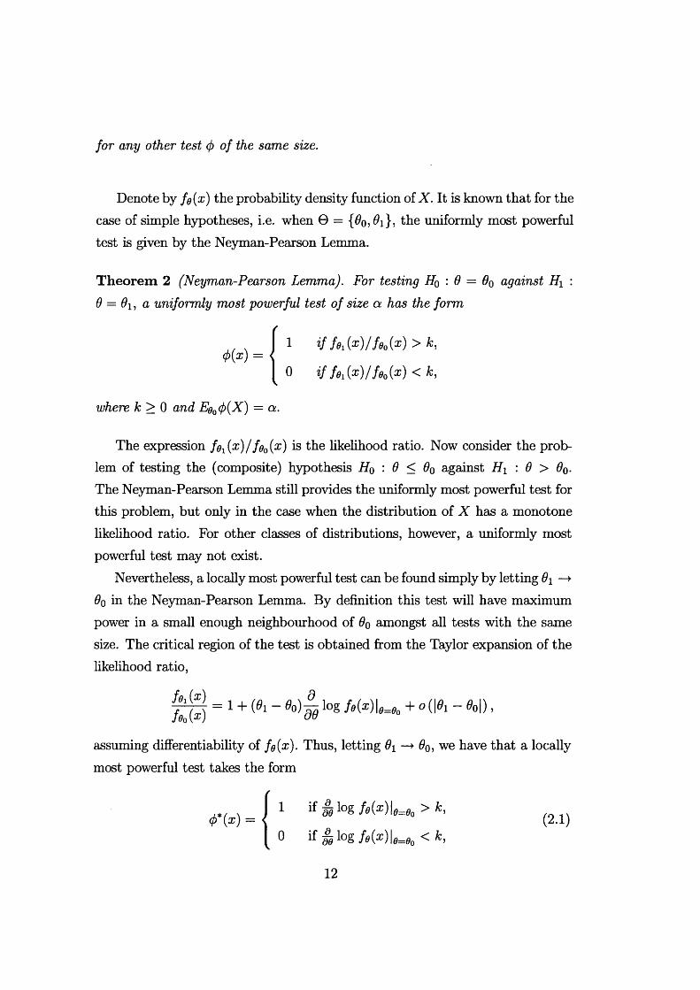
fo r any other test <j) o f the same size.

Denote by fg(x) the probability density function of X. It is known that for the case of simple hypotheses, i.e. when © = {#o5 the uniformly most powerful test is given by the Neyman-Pearson Lemma.

T heorem 2 (Neyman-Pearson Lemma). For testing H0 : 9 = 90 against H\ : 9 = 6i, a uniformly most powerful test of size a has the form

, , 1 if fe iW /fooix) > k,</>(x) =

0 tf feAx )/fe„(z) < k,

where k > 0 and Eg0<j)(X) = a.

The expression fgx (a:) / fg0 (x) is the hkelihood ratio. Now consider the prob­lem of testing the (composite) hypothesis H0 : 9 < 90 against Hi : 9 > 90. The Neyman-Pearson Lemma still provides the uniformly most powerful test for this problem, but only in the case when the distribution of X has a monotone likelihood ratio. For other classes of distributions, however, a uniformly most powerful test may not exist.

Nevertheless, a locally most powerful test can be found simply by letting 9\ —> 9q in the Neyman-Pearson Lemma. By definition this test will have maximum power in a small enough neighbourhood of 9q amongst all tests with the same size. The critical region of the test is obtained from the Taylor expansion of the likelihood ratio,

= 1 + (Q1 _ 0o) _ io g f g(x)\g=Qo + o(\9i - 0O|) ,

assuming differentiability of fe(x). Thus, letting 9i —> 90, we have that a locally most powerful test takes the form

1 if j k log f o ( x )\e= 90 >

0 if m l° s M x )\e=90 <

12

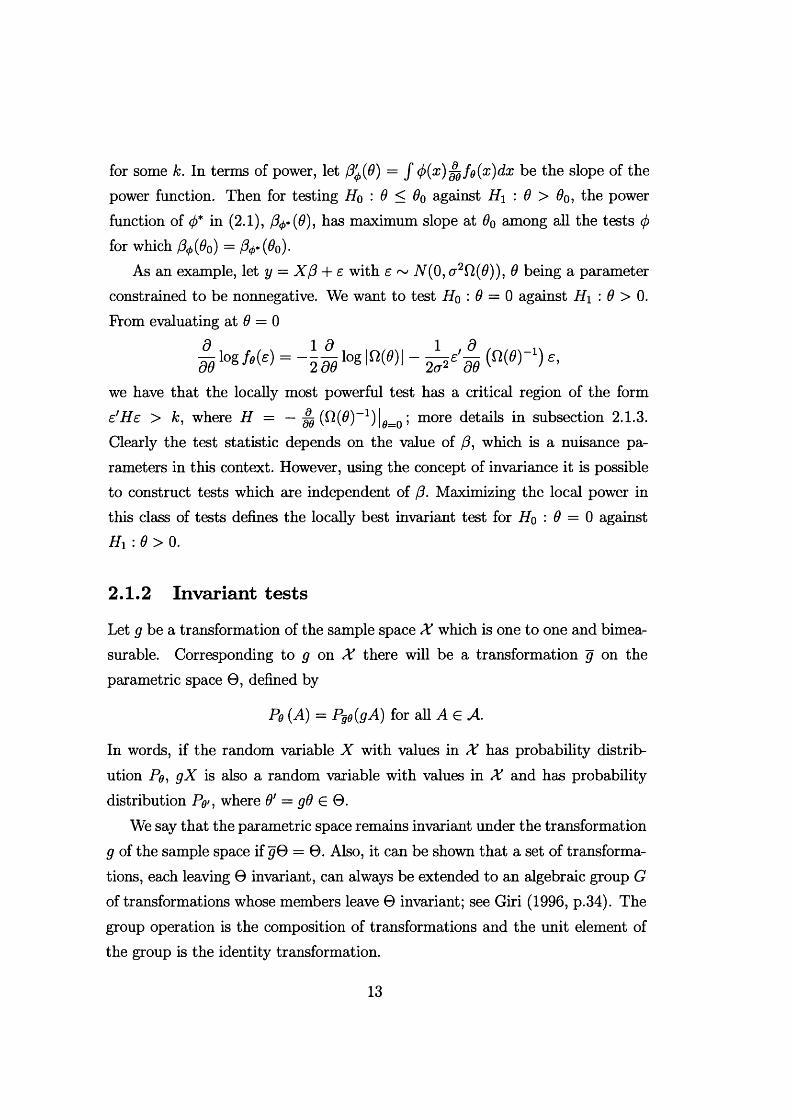
for some k . In terms of power, let (3^(0) = J <p{x)^fg{x)dx be the slope of the power function. Then for testing Hq : 6 < 6q against H\ : 0 > 0O, the power function of (f>* in (2.1), (3$* (0), has maximum slope at 60 among all the tests <j>

for which /^ (0O) = /V(#o)-As an example, let y = X(3 + e with e ~ N (0, <r2fl(0)), 6 being a parameter

constrained to be nonnegative. We want to test Ho : 6 = 0 against Hi : 9 > 0. From evaluating at 6 = 0

| log a m = log \ m \ - ^ 3 . (n (*)-i) e ,

we have that the locally most powerful test has a critical region of the form e'He > k , where H = — (fl(0)-1) |0=o; more details in subsection 2.1.3.Clearly the test statistic depends on the value of /?, which is a nuisance pa­rameters in this context. However, using the concept of invariance it is possible to construct tests which axe independent of (3. Maximizing the local power in this class of tests defines the locally best invariant test for Ho '• 0 = 0 against Hi : 0 > 0.

2.1.2 Invariant tests

Let g be a transformation of the sample space X which is one to one and bimea- surable. Corresponding to g on X there will be a transformation g on the parametric space 0 , defined by

Pe (A) = Pge(gA) for all A G A.

In words, if the random variable X with values in X has probability distrib­ution Pg, gX is also a random variable with values in X and has probability distribution Pg>, where O' = g6 G 0.

We say that the parametric space remains invariant under the transformation g of the sample space if gQ = 0 . Also, it can be shown that a set of transforma­tions, each leaving 0 invariant, can always be extended to an algebraic group G of transformations whose members leave © invariant; see Giri (1996, p.34). The group operation is the composition of transformations and the unit element of the group is the identity transformation.

13

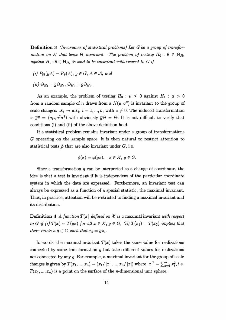
Definition 3 (Invariance of statistical problems) Let G be a group of transfor­mation on X that leave © invariant. The problem of testing Ho : 6 G Qh0 against Hi : 6 G is said to be invariant with respect to G if

(i) Pgg{gA) = Pe(A), g e G, A e A, and

(ii) Qh0 — 9®Ho j ®//i = 9®Hi •

As an example, the problem of testing H0 : (i < 0 against H\ : p > 0 from a random sample of n draws from a iV(/z, a2) is invariant to the group of scale changes: Xi —► aXi, i = 1, n, with a ^ 0. The induced transformation is £0 = (a/i,a2(r2) with obviously gQ = 0 . It is not difficult to verify that conditions (i) and (ii) of the above definition hold.

If a statistical problem remains invariant under a group of transformations G operating on the sample space, it is then natural to restrict attention to statistical tests (j> that are also invariant under G, i.e.

<f>(x) = <p(gx), x e X , g e G .

Since a transformation g can be interpreted as a change of coordinate, the idea is that a test is invariant if it is independent of the particular coordinate system in which the data are expressed. Furthermore, an invariant test can always be expressed as a function of a special statistic, the maximal invariant. Thus, in practice, attention will be restricted to finding a maximal invariant and its distribution.

Definition 4 A function T(x) defined on X is a maximal invariant with respect to G if (i) T{x) = T(gx) for all x G X , g G G , (ii) T (x i) = T (x2) implies that there exists a g G G such that X2 = gx\.

In words, the maximal invariant T{x) takes the same value for realizations connected by some transformation g but takes different values for realizations not connected by any g. For example, a maximal invariant for the group of scale changes is given by T(x 1, . . . ,rn) = (xi/ |x |, ...,xn/ |r |) where \x\2 = xh i-e* T(x 1,..., r n) is a point on the surface of the n-dimensional unit sphere.

14

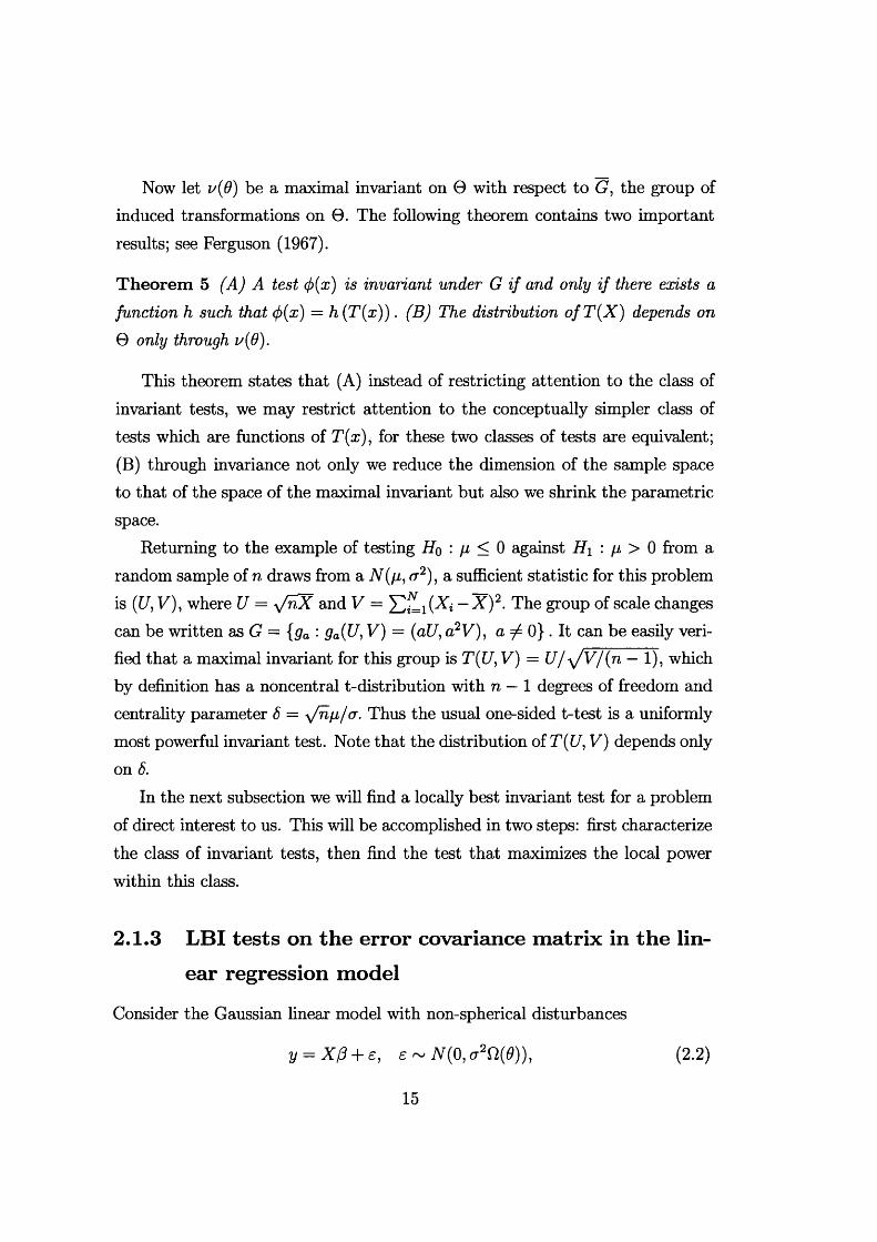
Now let v(Q) be a maximal invariant on © with respect to G, the group of induced transformations on 0 . The following theorem contains two important results; see Ferguson (1967).

Theorem 5 (A) A test <j)(x) is invariant under G if and only if there exists a function h such that (j>{x) = h{T (x )). (B) The distribution o fT (X ) depends on 0 only through v(0).

This theorem states that (A) instead of restricting attention to the class of invariant tests, we may restrict attention to the conceptually simpler class of tests which are functions of T(x), for these two classes of tests are equivalent; (B) through invariance not only we reduce the dimension of the sample space to that of the space of the maximal invariant but also we shrink the parametric space.

Returning to the example of testing Ho : p < 0 against Hi : p > 0 from a random sample of n draws from a N(p, a2), a sufficient statistic for this problem is (G, V), where U = yfnX and V = YliLi(Xi — X ) 2. The group of scale changes can be written as G = {ga : ga{U, V) = (aU, a2V), a ^ 0} . It can be easily veri­fied that a maximal invariant for this group is T(U,V) = U/ y /V /(n — 1), which by definition has a noncentral t-distribution with n — 1 degrees of freedom and centrality parameter <5 = y/np/a. Thus the usual one-sided t-test is a uniformly most powerful invariant test. Note that the distribution of T(U, V) depends only on 8.

In the next subsection we will find a locally best invariant test for a problem of direct interest to us. This will be accomplished in two steps: first characterize the class of invariant tests, then find the test that maximizes the local power within this class.

2.1.3 LBI tests on the error covariance m atrix in th e lin­

ear regression model

Consider the Gaussian linear model with non-spherical disturbances

y = X/3 + e, £ ~ N(0,<r2n(6)), (2.2)

15

where y is n x 1, X is a n x k matrix of fixed regressors with rank k , (3 and a2 are unknown parameters, and 17(0) is a symmetric positive definite matrix for all 9 > 0. Assume without loss of generality that 17(0) = In. The problem is testing Ho : 9 = 0 against Hi : 6 > 0.

The problem is invariant under the group of transformations G = {g : g(y) = ay + X b , a > 0, b € as can be seen from definition 3. To find the maximal invariant under G we can proceed in two steps.

First consider the group G\ = {g\ : gi{y) = y + Xb, b € An invariant function under G\ is M y, where M = In—X (X 'X )~ 1X ', since M y = M (y+Xb). Clearly M y is not a maximal invariant, as the dimension of the null space of M is k > 0. To find a maximal invariant, consider the decomposition M = PP' where P is a n x (7?, — k) matrix such that P 'P = In-k> Then z = P 'M y = P'y is a maximal invariant under G\. As z ~ N(0,o-2P'Q,(6)P), it is not difficult to see that a locally most powerful test invariant under G\ has a rejection region of the form y'M H M y > k, where H = — (^(0)_1) |0=o = Notethat M y are the OLS residuals from regressing y on X. However this test is not operative as its distribution depends on the unknown parameter a2.

Consider now the group G2 = {<72 • #2 (z) = az, a > 0}. As we have already seen, a maximal invariant under G2 is z j \z\ , i.e. a point on the surface of the unit sphere. Then, since G = {(72 0 <7i • gi £ G\, <72 G G2}, we have that a maximal invariant under G is

P ’M y P'yv = ------------------r = ---------- r-

(y'M P P 'M y)2 (y'M y) 2

Kariya (1980) and King (1980) show that the probability density function of v is (with m — n — k)

mfe(v)dv = | r ( |m ) tt"^ |P 'fi(0) P p (v' (P 'fi(0)P )_1 v j 2 dv, (2.3)

where dv denotes the uniform measure on the surface of the m-dimensional unit sphere.

From applying the Neyman-Pearson Lemma we see that a uniformly most powerful invariant test for Hq : 6 = 0 against Hi : 9 = 6\ > 0 in general does

16

not exist as the critical region takes the form v1 (P'Q(9i)P)~1 v < k, that is it depends on 6\. However a locally best invariant test (jf as defined in (2.1) can be obtained. From evaluating at 9 = 0

, -j|imifnwn + f *(raWPr‘p f 1 p'(1(,)f*2 3 0 8 1 2 V> ( P ' U { 6 ) P y l V

recalling that Q(0) = In and using the definition of v, we see that the LBI test has a critical region of the form

y'M H M y> k,y* M y

where H = -§qQ(9)\q=q . Call e = M y the OLS residuals from regressing y on X.Then the critical region can also be written as

^ > k . (2.4)eleRemark 1 Kariya (1980) and King (1980) have also showed that (2.4) is the lo­cally best invariant test when the distribution of e is ”elliptically symmetric” un­der Hi, i.e. when density ofe is of the form f q(e) = |cr2f}(0) |-1 q (a~2£,Q>(9)~1£ ) , where q is a function on [0 ,oo) satisfying f q(x'x)dx = 1. Gaussianity is a spe­cial case; other examples include the multivariate t-distribution, the compound normal, the multivariate Cauchy.

We now show that the LBI test (2.4) is also one-sided LM test. The log- likelihood for (2.2) is

Ufi, <r2, e) = iog(2^ 2) -1 log |n(*)| - X („ _ x p f m - 1 (v - X 0 ) ,with

= - \ t r („ _ x p y m - 1 ( ^ n(0)) (y - X f i ■

Under Ho : 9 = 0, the maximum likelihood estimators of /?, <r2, 9 are respec­tively (the OLS estimator) (8 = ( X 'X ^ X 'y , a2 = n~le’e, 9 = 0. Thus

This last expression is also the Lagrange multiplier for maximizing £(/3,cr2,6) under the constraint 6 = 0. Since 6 is positive under the alternative hypothesis, we have that a large positive value of (2.5) provides evidence in favour of H\. Thus the critical region of the one-sided LM test is given by (2.4).

The following theorem summarizes the results of this subsection.

T heorem 6 (LBI test; King and Hillier, 1985). For model (2.2) a locally most powerful test of Hq \ 6 = 0 against H\ : 6 > 0 invariant under the group of transformations G = {g : g(y) = ay + X b , a > 0, b 6 5Rfc} is

1

0

e'e

e'e

where e = M y are the OLS residuals from regressing y on X , H = -§q£1(0) |0 ,and k > 0 is an appropriate critical value. Further, the test (jf is also one sided LM test.

2.2 State space models and the Kalman filter

Let yt be a (n x 1) vector of observations at time t, t = 1,..., T. In a state space model, yt is generated by the system

yt = ZtQtt + d t £ t , (2-6)

at = Gtott~ i + ct + Rtr]t, (2-7)

where the et and rjt are zero mean, serially and mutually uncorrelated ran­dom vectors with covariance matrices Ht and Qt, et is n-dimensional and rjt m-dimensional, at is the state vector of dimension m, and dt , ct, Zt, Gt, R t are nonstochastic vectors and matrices. The formulation of the model is completed by specifying the initial conditions on the state vector a0 =E(oq), Pq = Var(a0).

18

The Kalman filter is a recursive algorithm for computing the optimal esti-

t, i.e. based on all the observations up to time t. The estimator is optimal in

estimators. If the model is Gaussian the minimum is among all the estimators.Let at denote the optimal estimator of the state vector and let Pt denote its

mean square error. The Kalman filter is given by

where Ft = ZtPt\t-iZ't + Ht- (2.8)-(2.9) are called predictions equations, (2 .10)- (2.11) are called updating equations. The prediction error of yt is vt = yt — Z tCLt\t- i — dt , t = 1, ...,T. Its mean square error is Ft, which is also its uncondi­tional variance. The Vt s are often termed innovations since they represent the new information in the latest observation.

The matrices Zt, Gt, R t, Ht , Qt and the vectors dt, ct may contain unknown parameters to be estimated on the basis of the observed data. Collect them into a vector ip. Under Gaussianity the log-likelihood function can be written in the prediction error decomposition form as

which can be maximized using some numerical optimization algorithm.A time invariant model is one where the matrices Zt, Gt, Rt, Ht, Qt are

constant over time. For this model the initial conditions for the Kalman filter, a0 and Pq, are given by the unconditional mean and variance of a t, provided a t is a stationary process (in the sense that the eigenvalues of G are inside the unit circle). When at is non-stationary its unconditional distribution is not defined, and the initial conditions are obtained assigning a diffuse prior to o0, i.e. assuming ag = 0 and Pq = Klm with k —> oo. Modifications of the Kalman

mator of the state vector at time t based on the information available at time

the sense that it minimizes the mean square error within the class of the linear

(2.8)

(2.9)

(2.10)

(2.11)

M) = — log2* - l £ l o g | f i | - (2-12)

19

filter to deal with this situation are proposed by Ansley and Kohn (1985), de Jong (1991), Koopman (1997). In practice, however, when there are, say, d nonstationary elements in the state vector it is often possible to construct a proper distribution for ad, and thus the log-likelihood of (yd+i, •••, Vt ) conditional on (yi, ...,yd) is given by (2 .12) with the summations running from t = d + 1

instead of t = 1. If 2/1, ---,2/d are regarded as being fixed, this log-likelihood is an unconditional one.

As an example consider the univariate random walk plus noise model,

yt = at + et, Var(et) = <J2,

at - ctt-i + Vt, Var(rjt) = qo2,

where q is the signal-to-noise ratio. The Kalman filter can be written compactly as

at = { l-p D a t-i+ P tV u

Pt = l - l / W - i + 4 + 1),

with p* = Pt/a 2. Taking y\ as fixed permits to initialize the filter at t = 1 by ai = 2/1, p\ = 1. Alternatively, starting off at t = 0 with = k yields p{ —► 1

and <2i —> ?/i as k —> 00, which shows that the two procedures are equivalent. Furthemore, also the two likelihoods are equivalent as F-f1 —> 0 as k, —> 00 .

2.3 GLS estim ation using the Kalman filter

Let yt, t = 1,..., T, be a scalar time series generated by the model

yt = x'tfd + ut (2.13)

Ut = Ztat + £t (2.14)

at = Gtat-i + Vt, (2.15)

where xt is a k x 1 vector of nonstochastic regressors, f) is a k x 1 vector of unknown parameters and ut is an error term that has a state space representation as in the previous section. As regards the initial conditions, assume for the

20

moment that E(ao) = 0 and that Var(ao) is bounded. Write (2.13) in matrix notation as

Y = X (3+ U ,

where Y , X , U are obtained by stacking the T observations on ?/*, x't , ut. Let Q =E(UU'). The Generalised Least Squares (GLS) estimator of (3 is known to be (3 = { X 'n - ' x y 1 X 'n - 'Y . Harvey (1989, ch. 3) shows that (3 can be computed using the Kalman filter to diagonalize fi”1. The argument proceeds as follows.

It is known that there exists a lower diagonal matrix L with ones on the main diagonal and a diagonal matrix F such that

IT 1 = L’F~XL.

This decomposition is effectively performed by the Kalman filter, whose output is a set of serially uncorrelated innovations vt with variance Ft. Stacking the vt’s into a T x 1 vector V, we have that V = LU with E(VV') = diag (Fi, ..., Ft ) = F.

Now let X* = L X , Y* = LY , i.e. X* and Y* are obtained by running the Kalman Filter on X and Y. Then (3 can be computed as

ii? = X ^ F - 'V . (2.16)

As regards the maximum likelihood estimation of the full model (i.e. both the regression coefficient @ and the state space parameters ip) we have that

W ) = — log 2tt — ^ log |fi| — ^ (K — X/3)' fi-1 (Y — Xf3) (2.17)

= ~ log 2tt - l- log |F | - I (IT - X*/3)' F - 1 {Y* - X * 0 ).

Maximising £((3, ip) with respect to (3 yields the (unfeasible) GLS estimator (3(ip) defined in (2.16), with the concentrated likelihood given by

4(V0 := max^/3, f ) = log 2tt - 1 log |F | - l- V ’F~xV, (2.18)

where V = Y* — X*0(ip).The assumption of zero mean and bounded variance for a0 may be relaxed.

The case of unbounded variance (diffuse prior) can be handled as suggested in

21

the previous section, whereas a nonzero mean model can always be reduced to a model with zero mean for qq by the inclusion of extra regressors (see Harvey, 1989 p. 139).

An algorithm for maximising (2.17) is as follows. Given an initial guess 'ipo we can compute /3(ipo) and 4(^o) by running the Kalman filter. The starting value ipo is then updated by some numerical optimization procedure applied to (2.18), so to obtain ipi. Having obtained ip\, we iterate the previous steps and proceed until convergence of £c(ip). In the next section we provide a simple program that implements this stepwise optimization algorithm. In particular, it computes the maximum likelihood estimator in a regression model where the errors are random walk plus noise. The program runs under the matrix language Ox 2.0 of Doornik (1998) and it requires the additional package Ssfpack 2.2 of Koopman et al. (1998). This program constitutes the basis for the more complicated maximization of the likelihood in the dynamic panel data models of chapter 61 .

2.4 An Ox program for com puting the maxi­mum likelihood estim ator o f a regression model w ith local level errors

/ *

This program computes the maximum likelihood estimator of a regression model with local level errors,using numerical derivatives in the maximization of the likelihood. The program runs under Ox 2.0 with SsfPack 2.2.Note: the two variance parameters of the model aresigma_eta, sigma.epsilon.Here we construct the likelihood in terms of the transformed parameters vp = log(sigmas), since vp must not be constrained

1 The software STAMP 5.0 of Koopman et al. (1995) can easily estimate regressions with local level errors (and also local linear trends with stochastic seasonality and cycles), but it does not work with panel data.

22

to be greater than zero. Then we obtain the variances by taking exp(2*vp) or the standard deviations by taking exp(vp).* /

#include <oxstd.h>#import <maximize>#include <packages/ssfpack/ssfpack.h>likelihood (const vp, const plik, const pvsco, const pmhes); static decl s_my, s_mx, s_vz, s.betagls, s_varbeta, s.mphi, s_momega, s.msigma, s_var;

main (){decl vp, ir, lik;decl data =loadmat(f fput-file-name-with-data-here* ‘) ;// Insert the file name with data ordered as y, xi, X2, . . ., x s_my=data[] [0] ’; s_mx=data[] [1:] ’;s_mphi=<l;l>; // state space matricess_momega=zeros(2,2); // this just defines the dimension of omega s_msigma=<-l;0>; // diffuse prior on the state

/* Maximization of the Likelihood */ vp=log(<0.5; 1>) ; // initial valueslikelihood (vp,&lik, 0,0); // evaluate likelihood vp += 0.5*log(s_var); // scale starting values // Iterative maximization of the log-likelihood MaxControl (100,10,1);ir = MaxBFGS(likelihood, &vp, &lik, 0, 1);// N.B. 1 => NUMERICAL DERIVATIVES

23

11 0 => identity matrix as starting hessian print ( 1‘\n‘( ,MaxConvergenceMsg(ir),‘ ‘\nlog-likelihood = lik*columns(s_my),‘‘\nvar = “ , s_var,‘‘\nparameters = 11, vp,‘‘\nomega = <f, s_momega);print (‘ e\nBeta_GLS = ‘ ‘ ,s_betagls,‘‘\n‘‘,‘‘\nVariance = f‘,s_varbeta,‘ <\n<‘,f‘\n\n t-value = ‘‘, s_betagls./(diagonal(s.varbeta.A0.5)*) ); }

likelihood (const vp, const plik, const pvsco, const pmhes){ // arguments dictated by MaxBFGSs_momega[0][0]=exp(2*vp[0][0]);// sigma-square_eta s_momega[l][l]=exp(2*vp[l] [0]);// sigma-square.epsilon decl mkf, vy, mvx=s_mx, vft, i;// This will compute KF innovations for y and x mkf = KalmanFil (s_my, s_mphi, s_momega, s.msigma); vy = mkf [0] [] ;vft = mkf[2][]; // this contains INVERSE of mse prediction for (i=0; i<rows(s_mx); ++i){mvx[i] [] = KalmanFil(s_mx[i] [] , s_mphi, s_momega, s_msigma) [0] [] ; }vy=dropc(vy,0); // drop first column (observation) as it mvx=dropc(mvx,0); // doesn't contain proper KF innovation vft=dropc(vft,0);s_betagls = ( ((mvx.’t'vft^mvx') A(-l) ) * ((mvx.+vft^vy'); s_varbeta = ((mvx.+vft^mvx') A(-l); s_vz = s_my - s_betagls'*s_mx;SsfLik (plik, &s_var, s_vz, s_mphi, s_momega, s.msigma);

24

// concentrated log-likelihood of our state space model plik[0] /= columns(s_vz); // loglik scaled by sample size return 1;}

25

Chapter 3

Testing for a stochastic trend in univariate tim e series

This chapter considers tests for the presence of a random walk component (sto­chastic trend) in a stationary or trend stationary time series and extends them to series which contain structural breaks. The tests fit the LBI framework de­scribed in the previous chapter.

Original contribution is provided in analyzing the case of series with struc­tural breaks. This analysis is important because the tests for stochastic trend have high power also against alternative hypotheses in which the trend of the series contains a small number of breaks but is otherwise deterministic. Thus, if structural breaks are known to be present, it is vital to take account of them if a test for a random walk component is to be carried out. This argument parallels Perron (1989) who shows how the augmented Dickey Fuller test needs to be modified in the case of breaking trends. The difference with respect to Perron is that the roles of the null and the alternative hypotheses are reversed, as in our tests the null is (trend) stationarity as opposed to unit root.

We derive the LBI test in the case of structural breaks and we also propose a simple modification of it. The advantage of this modified statistic is that its asymptotic distribution is not dependent on the location of the breakpoint and its form is that of the generalised Cramer-von Mises distribution, with degrees of freedom depending on the number of breakpoints. This is important, since although it may be feasible to tabulate critical values for a single break at different points in the sample, constructing tables where there are two or more

26

breaks is impractical. The performance of this modified test is shown, via some simulation experiments, to be comparable to that of the LBI test.

An unconditional test, based on the assumption that there is a single break at an unknown point is also examined. The test is obtained by choosing the breakpoint that gives the most favourable result for the null hypothesis of trend stationarity using the LBI statistic, i.e. it parallels the argument of Zivot and Andrews (1992) regarding the endogenization of the breakpoint in the Perron’s test.

Then we consider parametric and non-parametric corrections to be applied to our test statistics for handling serial correlation, we highlight some extensions and we provide some empirical examples with data on the flow of the Nile and with US GNP.

In summary, the chapter proceeds as follows. Section 3.1 considers the LBI test for the presence of a random walk component and section 3.2 its modification for the case of structural breaks. The asymptotic distribution is derived and the critical values are tabulated. The modified statistic and the unconditional test are the object of sections 3.3 and 3.4 respectively, with the appropriate critical values being tabulated. The correction for serial correlation is in section 3.5, some extensions in 3.6 and the empirical examples in 3.7. Finally, section 3.8 contains the proofs of this chapter’s propositions.

3.1 The LBI test for a random walk com ponent

Consider the model (t = 1,

yt = x't/3+nt + £t, (3.1)

ALt — + ( 3 *2 )

et ~ NID{0,<t2), (3.3)

Tfc ~ N ID (0 ,o2v), (3.4)

where xt is a set of nonstochastic regressors (including a constant) with co­efficients /?, et and Tjt are mutually independent, and /io = 0. The notation N ID (0,cr2) denotes normally and independently distributed with mean zero

27

and variance cr2. If a2n > 0, fit is a random walk component or stochastic trend. The objective is to test for Hq : cr2 = 0 against Hi \ <r2n > 0, i.e. to test for the presence of a random walk component.

By letting 6 = (r^/a2, it is clear that (3.1)-(3.4) falls into the class of models of chapter 2, equation (2.2), with Q(6) = IT + 6H and H being a T x T matrix whose element of position (s, t) is min(s, t). We will sometimes call 6 the signal- to-noise ratio and H the random walk generating matrix.

Theorem 6 of chapter 2 then provides the locally best invariant (LBI) test for Hq : a2v = 0 against Hi : > 0, where invariance is with repect to the groupof transformations G = {g : g(yt) = ayt + x'tb, a > 0, b G t = 1,..., T}. The test is also a one-sided Lagrange Multiplier test.

On dividing by the sample size T, we obtain the statistict t

E ( £ e s)2(3-5)

where the e*’s are the OLS residuals from regressing yt on xt and a2 — T~l Ylt= i e?*t t

Note that (3.5) is obtained because in our model e'He = X ^(S es)2* The LBIt = 1 5=1

test then rejects Hq : (j2v = 0 when £ > k, with k being an appropriate critical value.

The distribution of £ depends on the form of the regressors xt. Nyblom and Makelainen (1983) consider the simple case x t = 1, i.e. a random walk plus noise model. In this case, which we will refer to as NM test, we have that et = yt — y, where y is the sample mean. The asymptotic distribution of £ under the null hypothesis is found by first observing that the partial sum of deviations from the mean converges weakly to a standard Brownian bridge, that is

[T-]

5=1

where B (r) = W(r) — rW{ 1), r G [0,1], and W (‘) is a standard Wiener process or Brownian motion. Hence, by the continuous mapping theorem,

since a2 = T~l Ylt=i(Vt ~ y ) 2 <j2’ This asymptotic distribution is the well-known Cramer-von Mises distribution, as in Anderson and Darling (1952). We will denote it as CvM. Note that it is sufficient for the observations to be independent and identically distributed (and satisfy some moments conditions) to yield the result; see Nabeya and Tanaka (1988).

Nyblom (1986) augments the previous model by including a time trend (or drift), i.e. he considers the case x t = (1 ,t)'. For this case we have the analogous result that the partial sum of residuals from a first order polynomial regression converges weakly to a second level Brownian bridge denoted B2(-), where, as in McNeill (1978),

B 2(r) = W(r) — rW ( 1) + 6r (1 — r) |^W (1) — J W(s)ds

Thenf B 2(r)2d r . (3.7)

JoWe will refer to this asymptotic distribution as a second level Cramer-von Mises distribution, and denote it as CvM2. In the case of any ambiguity we will refer to the distribution in (3.6) as CvMi.

Percentage points for the Cramer-von Mises distribution have been tabulated by Anderson and Darling (1952), MacNeill (1978), Nyblom and Makelainen (1983), Nyblom (1986) and Kwiatkowski et al. (1992).

Kwiatkowski et al. (1992) have extended the above tests to allow et to be a weak dependent process (instead of a white noise). The idea is to correct the test statistic (3.5) nonparametrically by replacing a with a consistent estimator of the long run variance of et. Then the asymptotic distribution of the corrected statistic will be the same as the one derived under the assumption of white noise disturbances. This corrected version of the test will be denoted as KPSS test. The details on this and other procedures for handling serial correlation in et are contained in section 3.5.

One problem with the NM/KPSS tests is that they are consistent also against the alternative hypothesis of a level shift (and/or slope shift) in the series. This is indirectly shown in an early work of Gardner (1969) who derives the NM

29

statistic in a Bayesian framework to detect a break in an otherwise i.i.d. series. Later Nyblom (1989) derives (3.5) as an LM statistic to test a general form of parameter constancy in the mean of the series, namely for cases when under the alternative hypothesis the mean is a martingale (which includes both the cases of random walk and single shift at a randomly chosen point). Then Lee et al. (1997) show directly that the KPSS statistic diverges when there is a structural break in a (trend) stationary process. Therefore failing to account for a structural break when testing stationarity of a series is likely to produce evidence of nonstationarity1 .

To illustrate the problem, we consider the NM test when we assume that the true data generating process is

Vt = V o + 6wt + et

where wt = 1 (t > AT), A G (0,1), and et ~ NID(0, <r2). That is, the series is a white noise with a level shift at time r = [AT]. Since

yt - y = 6(wt - w ) + et - e i

we have that, for r G [0,1],

[ T r ]

T - i ' £ ( y t - y ) = O p ( T i ) .t = 1

Then, since T~l X lL ife “ V)2 = PpW> ^ follows that the statistic £ is Op(T) and so the NM test is consistent against the alternative hypothesis of a level shift in the series.

In the next section we show how the asymptotic distribution of the LBI test for a random walk component changes in the presence of (correctly modelled) structural breaks.

1 This corresponds to the Perron’s (1989) argument. Indeed Leybourne et al. (1999) have also showed the converse, i.e. that the presence of a break in a 1(1) series may lead to spurious rejections of the unit root hypothesis.

30

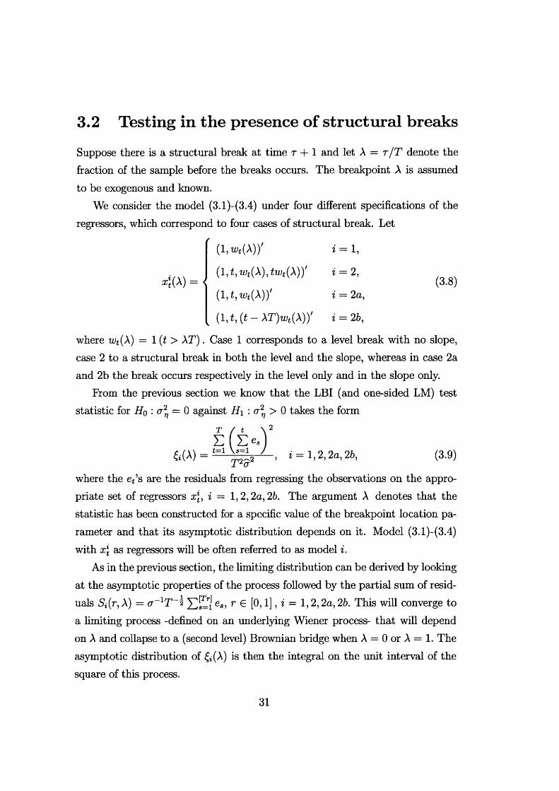
3.2 Testing in the presence o f structural breaks

Suppose there is a structural break at time t + 1 and let A = t / T denote the fraction of the sample before the breaks occurs. The breakpoint A is assumed to be exogenous and known.

We consider the model (3.1)-(3.4) under four different specifications of the regressors, which correspond to four cases of structural break. Let

z{(A) = <

(l,tuj(A))' i = 1,

( l , t ,w t(X),twt(\))' i = 2,(o.o)

( l , t ,w t(\))' i = 2a,

(1, t , (t - XT)wt(X))' i = 26,

where wt(A) = 1 (t > XT) . Case 1 corresponds to a level break with no slope, case 2 to a structural break in both the level and the slope, whereas in case 2a and 2b the break occurs respectively in the level only and in the slope only.

From the previous section we know that the LBI (and one-sided LM) test statistic for H0 : = 0 against Hi : (t2v > 0 takes the form

e ( x> » )t=1 \s=l /SiW = > i = 1,2,2a, 2b, (3.9)1 <7

where the et’s are the residuals from regressing the observations on the appro­priate set of regressors rrj, i = 1,2,2a, 26. The argument A denotes that the statistic has been constructed for a specific value of the breakpoint location pa­rameter and that its asymptotic distribution depends on it. Model (3.1)-(3.4) with x\ as regressors will be often referred to as model i.

As in the previous section, the limiting distribution can be derived by looking at the asymptotic properties of the process followed by the partial sum of resid­uals Si(r, A) = a~lT ~s ^ ^ [0,1], z = 1,2,2a, 26. This will converge toa limiting process -defined on an underlying Wiener process- that will depend on A and collapse to a (second level) Brownian bridge when A = 0 or A = 1. The asymptotic distribution of &(X) is then the integral on the unit interval of the square of this process.

31

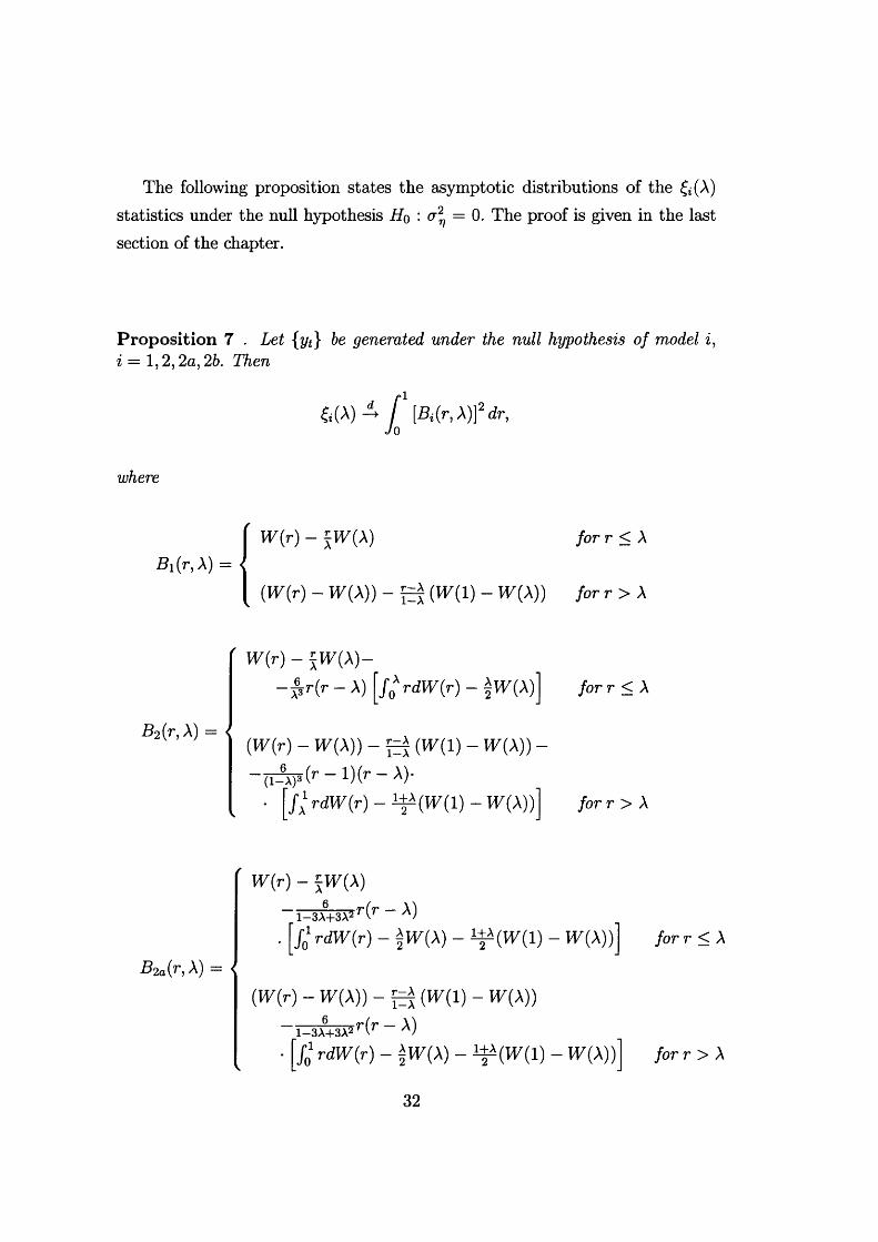
The following proposition states the asymptotic distributions of the &(A) statistics under the null hypothesis # 0 : ^ — 0. The proof is given in the last section of the chapter.

P roposition 7 . Let {yt} be generated under the null hypothesis of model i , i = 1,2,2a, 2b. Then

f [Bi(r,X)]2dr, Jo

where

B\{r, A) =W(r) - IW(X) for r < A

(W{r) - W(A)) - (W (l) - W(A)) f o r r > A

for r < A

(W(r) - W(A)) - (W( 1) - W(A)) -

J .1 rdW (r) - - W(A)) for r > X

B2a(r,X) = <

W {r) - JW(A)

1—3A+3A2 r (r —

'/o1 rdW (r ) - - ¥ W ! ) - W W ) for r < A

(W(r) - W(A)) - H W l ) - W'W) •(r - A)1—3A+3A2

£ r d ^ ( r ) - f l V ( A ) - ^ ( ^ ( 1 ) - W ( A )) /o r r > A

32

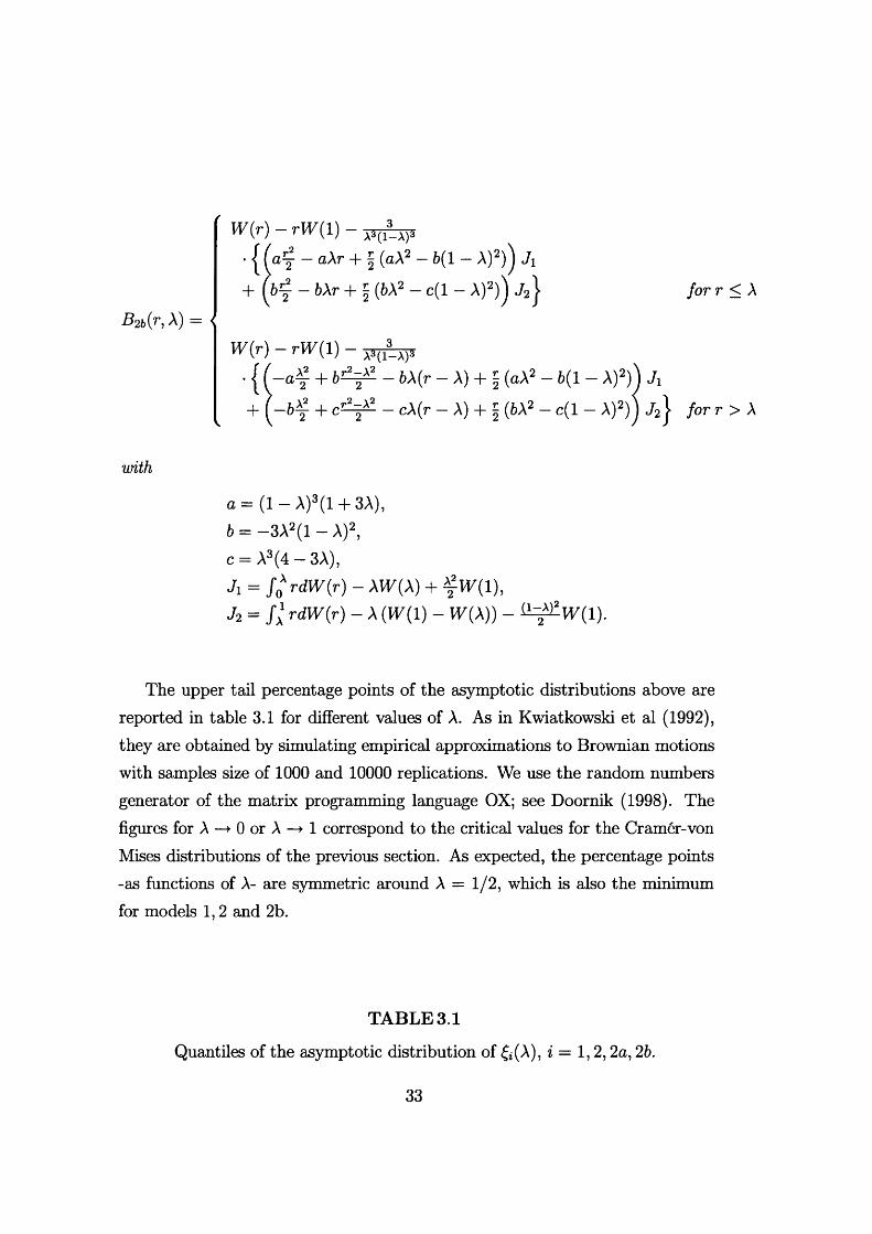
B2b(r, A) =

W(r) - rW ( 1) -

■ { ( a ^ - a \r + § (aA2 - 6(1 - A)2)) 7,

+ (& f - 6Ar + § (6A2 - c(l - A)2)) J2\

W{r) ~ rW ( 1) -

fo r r < A

!- a2 - b\(r - A) + | (aA2 - 6(1 - A)2) I Jx

+ ( —6 ^ + c7-2/ — cA(r — A) + | (6A2 — c(l — A)2) j J2} r > A

with

a — (1 — A)3(l + 3A),6 = —3A2(1 - A)2, c = A3(4-3A ),7! = / 0Ar<W (r) - AW(A) + %W(1), J2 = / 1 rdW(r) - A (W (l) - W(A)) W ( 1).

The upper tail percentage points of the asymptotic distributions above are reported in table 3.1 for different values of A. As in Kwiatkowski et al (1992), they are obtained by simulating empirical approximations to Brownian motions with samples size of 1000 and 10000 replications. We use the random numbers generator of the matrix programming language OX; see Doornik (1998). The figures for A —> 0 or A —> 1 correspond to the critical values for the Cramer-von Mises distributions of the previous section. As expected, the percentage points -as functions of A- are symmetric around A = 1/2, which is also the minimum for models 1,2 and 2b.

TABLE 3.1

Quantiles of the asymptotic distribution of &(A), i = 1 ,2 ,2a, 26.

33

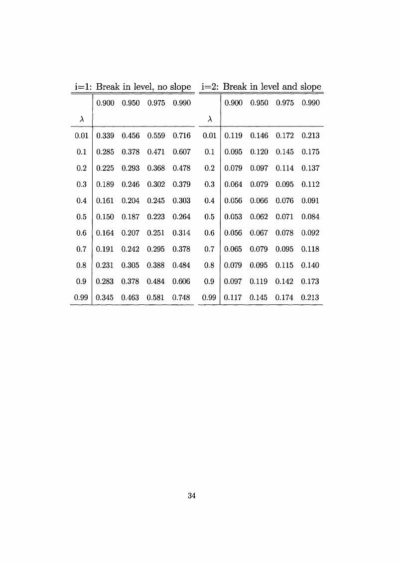
i= l: Break in level, no slope i=2: Break in level and slope

A

0.900 0.950 0.975 0.990

A

0.900 0.950 0.975 0.990

0.01 0.339 0.456 0.559 0.716 0.01 0.119 0.146 0.172 0.213

0.1 0.285 0.378 0.471 0.607 0.1 0.095 0.120 0.145 0.175

0.2 0.225 0.293 0.368 0.478 0.2 0.079 0.097 0.114 0.137

0.3 0.189 0.246 0.302 0.379 0.3 0.064 0.079 0.095 0.112

0.4 0.161 0.204 0.245 0.303 0.4 0.056 0.066 0.076 0.091

0.5 0.150 0.187 0.223 0.264 0.5 0.053 0.062 0.071 0.084

0.6 0.164 0.207 0.251 0.314 0.6 0.056 0.067 0.078 0.092

0.7 0.191 0.242 0.295 0.378 0.7 0.065 0.079 0.095 0.118

0.8 0.231 0.305 0.388 0.484 0.8 0.079 0.095 0.115 0.140

0.9 0.283 0.378 0.484 0.606 0.9 0.097 0.119 0.142 0.173

0.99 0.345 0.463 0.581 0.748 0.99 0.117 0.145 0.174 0.213

34

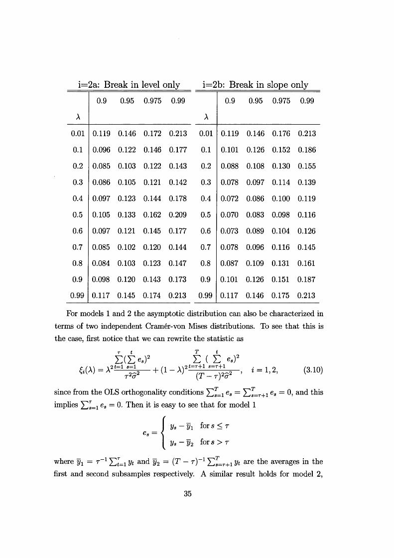
i=2a: Break in level only i—2b: Break in slope only

A

0.9 0.95 0.975 0.99

A

0.9 0.95 0.975 0.99

0.01 0.119 0.146 0.172 0.213 0.01 0.119 0.146 0.176 0.213

0.1 0.096 0.122 0.146 0.177 0.1 0.101 0.126 0.152 0.186

0.2 0.085 0.103 0.122 0.143 0.2 0.088 0.108 0.130 0.155

0.3 0.086 0.105 0.121 0.142 0.3 0.078 0.097 0.114 0.139

0.4 0.097 0.123 0.144 0.178 0.4 0.072 0.086 0.100 0.119

0.5 0.105 0.133 0.162 0.209 0.5 0.070 0.083 0.098 0.116

0.6 0.097 0.121 0.145 0.177 0.6 0.073 0.089 0.104 0.126

0.7 0.085 0.102 0.120 0.144 0.7 0.078 0.096 0.116 0.145

0.8 0.084 0.103 0.123 0.147 0.8 0.087 0.109 0.131 0.161

0.9 0.098 0.120 0.143 0.173 0.9 0.101 0.126 0.151 0.187

0.99 0.117 0.145 0.174 0.213 0.99 0.117 0.146 0.175 0.213

For models 1 and 2 the asymptotic distribution can also be characterized in terms of two independent Cramer-von Mises distributions. To see that this is the case, first notice that we can rewrite the statistic as

r t

E (E e»)2 E ( E e*)26(A) = A2t=1 % + (1 - A)2l=T+1 s=T+l-*/Tr*cr (T — t ) 2<t 2 ’

T

* = 1, 2, (3.10)

since from the OLS orthogonality conditions Xls=i e« = S s=r+i e« = 0, and this implies es = 0- Then it is easy to see that for model 1

e- = <V s-V i for s < r

ys - y 2 for s > r

where y1 = t 1 y t and y2 = ( T - r ) 1 X)J=T+1 y t are the averages in the first and second subsamples respectively. A similar result holds for model 2,

35

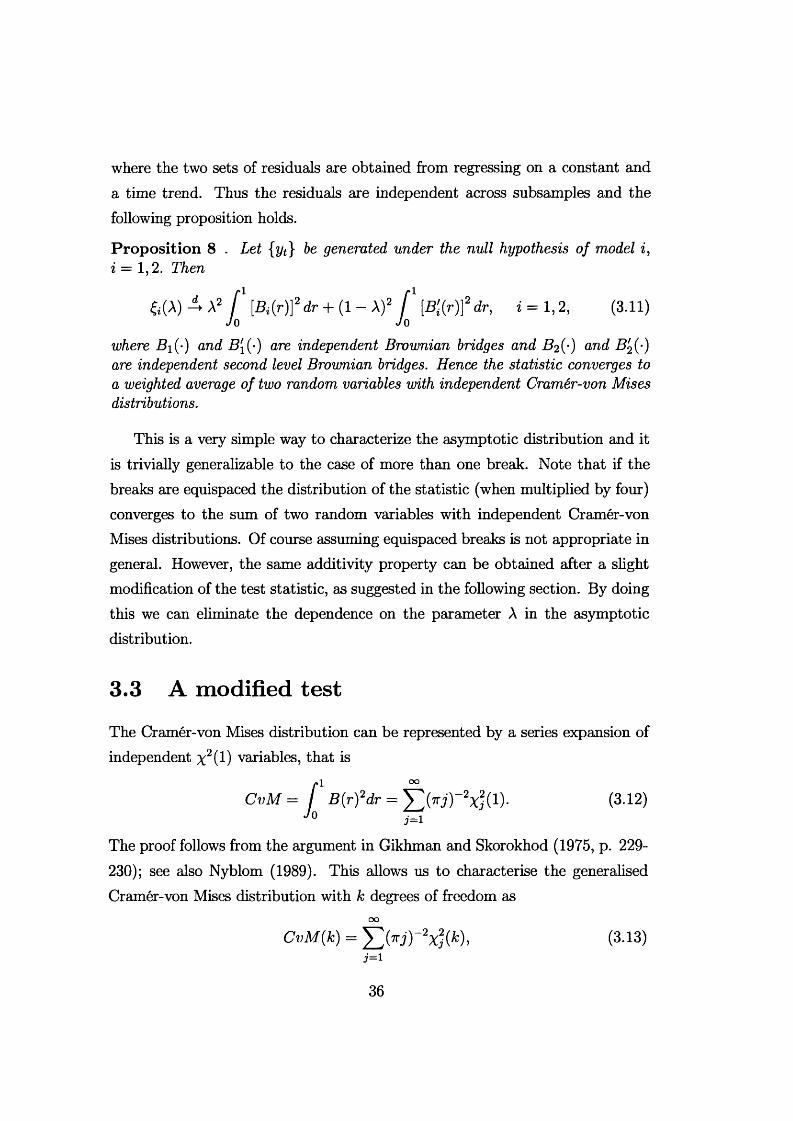
where the two sets of residuals are obtained from regressing on a constant and a time trend. Thus the residuals are independent across subsamples and the following proposition holds.

P roposition 8 . Let {yt} be generated under the null hypothesis of model z, z = 1,2. Then

&(A) 4 A2 f [B i ( r )]2 dr + ( 1 - A)2 f [B'(r)]2 dr, * = 1,2, (3.11)Jo Jo

where B\{-) and B[(') are independent Brownian bridges and ^ (O and B'2(-) are independent second level Brownian bridges. Hence the statistic converges to a weighted average of two random variables with independent Cramer-von Mises distributions.

This is a very simple way to characterize the asymptotic distribution and it is trivially generalizable to the case of more than one break. Note that if the breaks are equispaced the distribution of the statistic (when multiplied by four) converges to the sum of two random variables with independent Cramer-von Mises distributions. Of course assuming equispaced breaks is not appropriate in general. However, the same additivity property can be obtained after a slight modification of the test statistic, as suggested in the following section. By doing this we can eliminate the dependence on the parameter A in the asymptotic distribution.

3.3 A modified test

The Cramer-von Mises distribution can be represented by a series expansion of independent x2(l) variables, that is

l 00B { r fd r = ^ ( 7 r j ) " 2x2(l)- (3.12)

The proof follows from the argument in Gikhman and Skorokhod (1975, p. 229-230); see also Nyblom (1989). This allows us to characterise the generalisedCramer-von Mises distribution with k degrees of freedom as

oo

CvM(k) = ^ ( 7 r? T 2Xj(fc), (3-13)3 =1

C v M = [ Jo

36

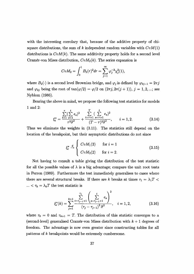
with the interesting corrolary that, because of the additive property of chi- square distributions, the sum of k independent random variables with CvM( 1) distributions is CvM(k). The same additivity property holds for a second level Cramer-von Mises distribution, CvM 2 (k). The series expansion is

/•i °°CvM2 = / B2(r)2dr = y2<pj2x 2j (i),

J o 4=13 = J

where is a second level Brownian bridge, and is defined by = 27xj and (p2j being the root of tan(<£>/2) = cp/2 on (27rj,27r(j + 1)), j = 1 , 2 , see Nyblom (1986).

Bearing the above in mind, we propose the following test statistics for models 1 and 2 :

E(X>*)2 E ( E «.)’S = t=1 7^2 + ‘=T,*! a=T;~ 2 . < = 1. 2- (3-14)

T l (T ( T — T ) 2 (T

Thus we eliminate the weights in (3.11). The statistics still depend on the location of the breakpoint, but their asymptotic distributions do not since

CvM\(2) for i — 1(3.15)

CvM 2 (2 ) for i = 2.

Not having to consult a table giving the distribution of the test statistic for all the possible values of A is a big advantage; compare the unit root tests in Perron (1989). Furthermore the test immediately generalises to cases where there are several structural breaks. If there are k breaks at times T\ = AiT < ... < Tk = AkT the test statistic is

*+1 E ( E e.)y . % ^ t Tfl 1 ”|“ 1 \ 8 T7 — 1 “(“ 1 /

«?(*) = E -----3 ^ - , < = 1,2, (3.16)

where tq = 0 and r^+i = T. The distribution of this statistic converges to a (second-level) generalised Cramer-von Mises distribution with k + 1 degrees of freedom. The advantage is now even greater since constructing tables for all patterns of k breakpoints would be extremely cumbersome.

37

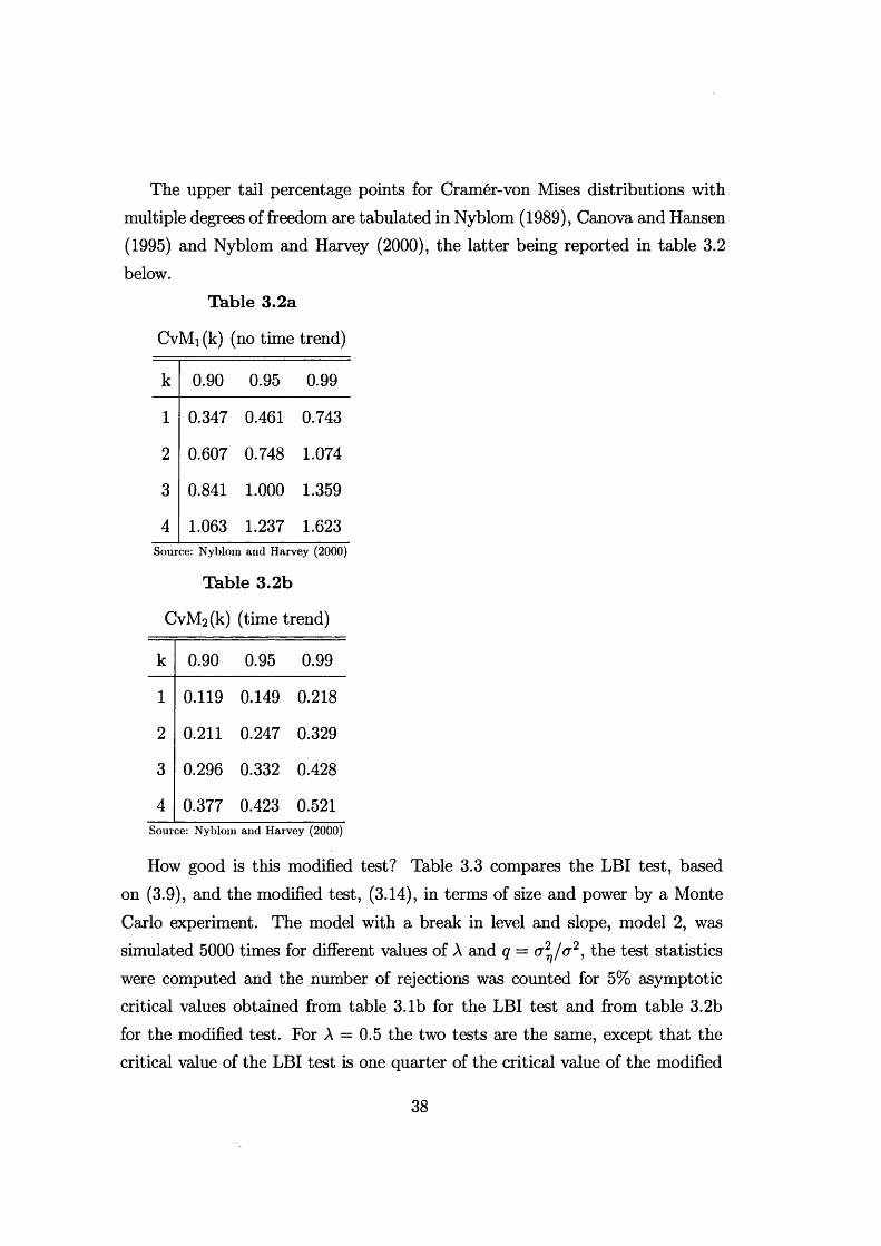
The upper tail percentage points for Cramer-von Mises distributions with multiple degrees of freedom are tabulated in Nyblom (1989), Canova and Hansen (1995) and Nyblom and Harvey (2000), the latter being reported in table 3.2 below.

Table 3.2a

CvMi (k) (no time trend)

k 0.90 0.95 0.99

1 0.347 0.461 0.743

2 0.607 0.748 1.074

3 0.841 1.000 1.359

4 1.063 1.237 1.623Source: Nyblom and Harvey (2000)

Table 3.2b

CvM2(k) (time trend)

k 0.90 0.95 0.99

1 0.119 0.149 0.218

2 0.211 0.247 0.329

3 0.296 0.332 0.428

4 0.377 0.423 0.521Source: Nyblom and Harvey (2000)

How good is this modified test? Table 3.3 compares the LBI test, based on (3.9), and the modified test, (3.14), in terms of size and power by a Monte Carlo experiment. The model with a break in level and slope, model 2, was simulated 5000 times for different values of A and q = cr^/v2, the test statistics were computed and the number of rejections was counted for 5% asymptotic critical values obtained from table 3.1b for the LBI test and from table 3.2b for the modified test. For A = 0.5 the two tests are the same, except that the critical value of the LBI test is one quarter of the critical value of the modified

38

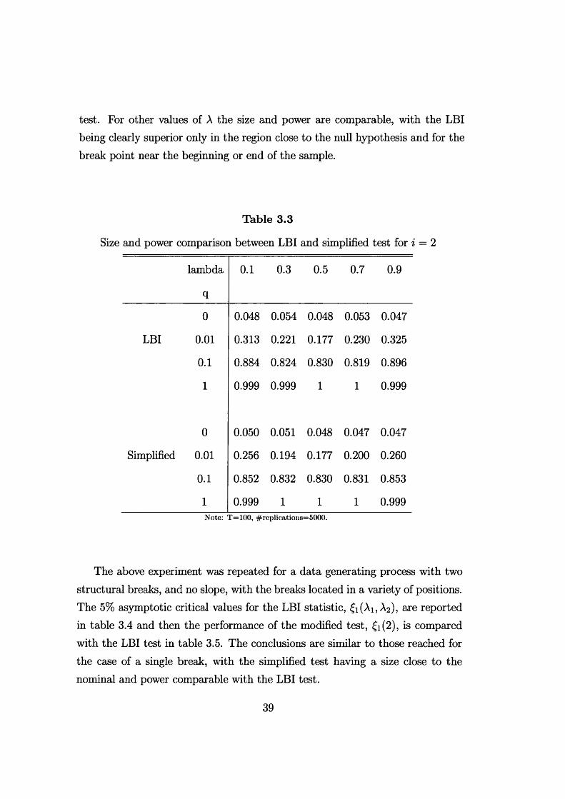
test. For other values of A the size and power are comparable, with the LBI being clearly superior only in the region close to the null hypothesis and for the break point near the beginning or end of the sample.

Table 3.3

Size and power comparison between LBI and simplified test for i = 2

lambda

q

0.1 0.3 0.5 0.7 0.9

0 0.048 0.054 0.048 0.053 0.047

LBI 0.01 0.313 0.221 0.177 0.230 0.325

0.1 0.884 0.824 0.830 0.819 0.896

1 0.999 0.999 1 1 0.999

0 0.050 0.051 0.048 0.047 0.047

Simplified 0.01 0.256 0.194 0.177 0.200 0.260

0.1 0.852 0.832 0.830 0.831 0.853

1 0.999 1 1 1 0.999Note: T=10(), #replications=5000.

The above experiment was repeated for a data generating process with two structural breaks, and no slope, with the breaks located in a variety of positions. The 5% asymptotic critical values for the LBI statistic, fi(Ai, A2), are reported in table 3.4 and then the performance of the modified test, £i(2), is compared with the LBI test in table 3.5. The conclusions are similar to those reached for the case of a single break, with the simplified test having a size close to the nominal and power comparable with the LBI test.

39

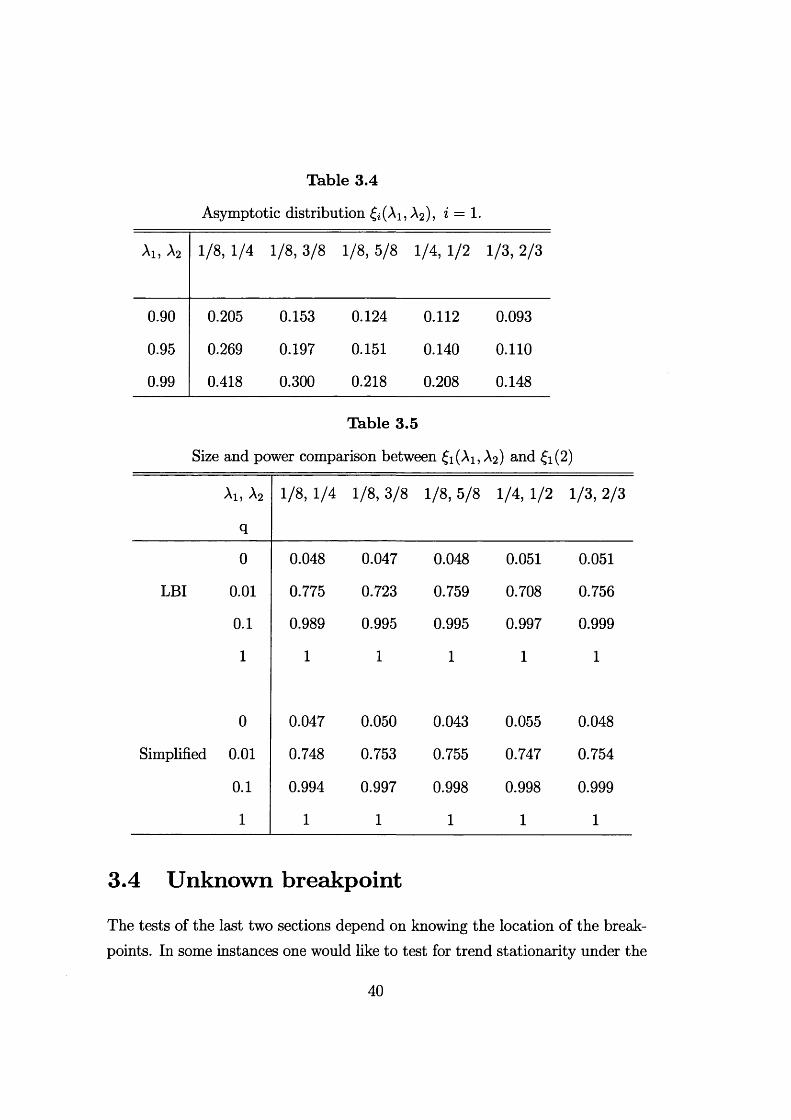
Table 3.4

Asymptotic distribution fi(A1? A2), i = 1.

Ai, A2 1/8, 1/4 1/8, 3/8 1/8, 5/8 1/4, 1/2 1/3, 2/3

0.90 0.205 0.153 0.124 0.112 0.093

0.95 0.269 0.197 0.151 0.140 0.110

0.99 0.418 0.300 0.218 0.208 0.148

Table 3.5

Size and power comparison between fi(Ai, A2) and £i(2)

Ai, A2

q

1/8, 1/4 1/8, 3/8 1/8, 5/8 1/4, 1/2 1/3, 2/3

0 0.048 0.047 0.048 0.051 0.051

LBI 0.01 0.775 0.723 0.759 0.708 0.756

0.1 0.989 0.995 0.995 0.997 0.999

1 1 1 1 1 1

0 0.047 0.050 0.043 0.055 0.048

Simplified 0.01 0.748 0.753 0.755 0.747 0.754

0.1 0.994 0.997 0.998 0.998 0.999

1 1 1 1 1 1

3.4 Unknown breakpoint

The tests of the last two sections depend on knowing the location of the break­points. In some instances one would like to test for trend stationarity under the

40

assumption that there may be a single break in an unknown position.For a single structural break at an unknown point, we consider a set of

unconditional tests, obtained by following the argument in Zivot and Andrews (1992). The idea is to choose the breakpoint that gives the most favourable result for the null hypothesis of trend stationarity using the £i(A ) statistic, that is

& =inf& (A), i = 1, 2 , 2a, 26, (3.17)A€A

where A is a closed subset of the interval (0 ,1).The distribution of will depend not only on the location of the true break­

point, denoted Ao, but also on the magnitude of the level and/or slope shift, because each & (A) statistic will depend on the latter when it is computed for a breakpoint different from Ao- The following assumption on the magnitude of the shift allows us to derive the asymptotic distribution of

Shift assum ption. The magnitude of the shifts decreases to zero with the sample size at a rate faster than T~1 2 for the level shifts and at a rate faster than T ~3/ 2 for the slope shifts.

Whether this assumption is a reasonable one is open to question. However, in the literature on breakpoint estimation, Bai (1994, 1997) assumes that the magnitude of the shift shrinks to zero at a rate slower than T~1//2 in order to derive the asymptotic distribution of the breakpoint estimator. In our case, the rate is faster. Note that the assumption covers the case of no break actually occuring.

P roposition 9 . Let {yt} be generated under the null hypothesis of model i, i = 1, 2 , 2a, 2b. Under the above shift assumption

& A)l2 d r’ i = -1’2’2a’26’Jo

where Bi(r , A) is defined as in proposition 1.

The proposition is proved in the last section of the chapter. First we prove that, under the shift assumption, the asymptotic distribution of proposition 7 still holds when the location of the breakpoint is wrongly assumed. Then it

41

is sufficient to apply the continuous mapping theorem as in Zivot and Andrews (1992) to get the result. Note that a co-integration test corresponding to case 1 is proposed by Hao (1996), but he does not apparently make the shift assumption.

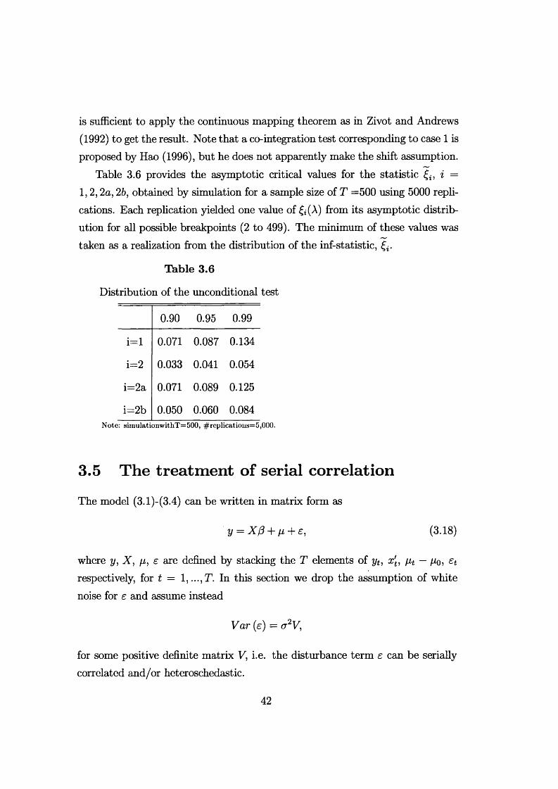
Table 3.6 provides the asymptotic critical values for the statistic f i} i = 1,2 ,2a, 26, obtained by simulation for a sample size of T =500 using 5000 repli­cations. Each replication yielded one value of £i(A ) from its asymptotic distrib­ution for all possible breakpoints (2 to 499). The minimum of these values was taken as a realization from the distribution of the inf-statistic,

Table 3.6

Distribution of the unconditional test

0.90 0.95 0.99

i= l 0.071 0.087 0.134

i= 2 0.033 0.041 0.054

• II to p 0.071 0.089 0.125

i= 2b 0.050 0.060 0.084Note: simulationwit.hT=500, #replications=5,()00.

3.5 The treatm ent o f serial correlation

The model (3.1)-(3.4) can be written in matrix form as

y = X/3 + // + £, (3.18)

where y, X, /i, e are defined by stacking the T elements of yt, x't, fit — /io, £trespectively, for t = 1,...,T. In this section we drop the assumption of whitenoise for e and assume instead

Var (e) = cr2V,

for some positive definite matrix V, i.e. the disturbance term e can be serially correlated and/or heteroschedastic.

42

The test defined by the statistic £ in (3.5) is now biased, in that the asymp­totic distribution of £ is only proportional to the one corresponding to the case of white noise disturbances, the factor of proportionality being related to the spectrum at frequency zero of e (or long run variance of e). Kwiatowski, Phillips, Schmidt and Shin (1992) therefore corrects £ using a nonparametric estimator of the spectrum at zero. Such (nonparametric) correction is often termed KPSS correction and is described in the first subsection below. Note that the corrected test is no longer LBI.

A different approach to dealing with serial correlation is to compute the LBI test for the model (3.18) using a consistent estimator of V. In fact, after premultiplying (3.18) by V ~%, we can still apply theorem 6 of chapter 2 to obtain the LBI test for the presence of a random walk component. The rejection region now takes the form

? V - lH V ~le , / o _

y v - ' e > ’ ( ^where A; is a critical value, H is the random walk generating matrix and e is the vector of generalised least squares (GLS) residuals

= ( lT - x ( X ' V - ' x y 1 x ' v - 1) y .

This approach is parametric, since V needs to be estimated by parametrizing (and estimating) the model under H\. Leybourne and McCabe (1994) and Har­vey and Streibel (1997) follow this approach, that will be described in the second subsection below.

It can be conjectured that the parametric test is bound to be superior to the KPSS test in small samples, provided an appropriate model has been fitted to the data. In effect, simulation evidence in the two papers above shows this to be the case.

3.5.1 Nonparametric correction

By the invariance principle, under regularity conditions2 the partial sum process of the disturbances weakly converges to a standard Wiener process when stan­2 Details on the conditions under which the nonparametric correction works are given in the next chapter, section 4.2.

43

dardized by the square root of the long run variance a 1, i.e.

[Tv ]

a l 'T - l £ > => r e [o, 1], (3.20)t= 1

where the long run variance is defined as

^ = r is , b V a r f e £t j • (3-21)

An estimator for cr\ is given by

m

«2(m) = 5 2 “'(•?> m)W)>j = —m

where w(j, m) is a weighting function and 7 (j) is the sample autocovariance of the OLS residuals at lag j,

T

7 0 ') = T~lt = j + 1

Here we use w(j,m) = 1 — \j\ /(m + 1); other options are examined e.g. in Andrews (1991). For consistency it is required that m —> 00 at a rate slower than T; see chapter 4 section 4.2.

Using (3.20) it follows that the LBI test statistic (3.5) can be corrected by replacing a2 with s2(m) to yield the KPSS statistic

t t

E ( X > .) 2

^KPSS = ‘ ^ ( m ) ' (3'22)

Clearly the KPSS statistic has the same asymptotic distribution as the corre­sponding LBI statistic for white noise disturbances; the details are given in the next chapter that considers this same problem in the multivariate case.

3.5.2 Param etric correction

Harvey and Streibel (1997) work with the LBI test (3.19) from a state-space approach. The model (3.18) can be easily put in state-space form and the

44

Kalman filter and the smoother can be applied to it. In particular, the smoother is an algorithm to compute the optimal estimator of the state based on all the observations; see Harvey (1989).

The numerator of (3.18) is a quadratic form in the Txl vector

u = V~le,

whose element are sometimes called smoothing errors. They are obtained di­rectly by the Kalman filter smoother withouth having to invert the TxT matrix V. An appropriate standardization of (3.19) then leads to the following statistic

£ ( X > » ) 2i n s = ‘- 1 ■ (3-23)

where 7 = T~ld2l'V ~ l \ emerges as a by-product of the Kalman smoother cal­culations; see Harvey and Streibel (1997) for the details. The asymptotic dis­tribution of (3.23) is the same as the one of the corresponding LBI statistic for white noise disturbances. Note that in practice the matrix V depends on unknown parameters that need to be estimated. Harvey and Streibel (1997) suggest to estimate them under Hi, by fitting an appropriate state space model. After estimation, the smoothing errors are obtained and the statistic (3.23) can be computed.

In the ARIMA framework, a parametric correction to the LBI statitic has been proposed by Leybourne and McCabe (1994). They allow for serial corre­lation by introducing lagged values of the dependent variable, i.e. they consider the model

= x'tP+Vt + St, (3-24)

fit = fit- 1 + Vt, (3.25)

where (fi(L) is an AR(p) polinomial with roots outside the unit circle. UnderHi : a2v > 0, the reduced form of (3.24)-(3.25) is an ARIMA(p,l,l) process.Leybourne and McCabe (1994) estimate the reduced form and construct the LBI statistic (3.5) using the residuals from regressing 4>(L)yt on xt , where (j>{L)

45

is the estimated AR polinomial obtained from the reduced form. Again, it can be shown that the critical values for this test are the same as the ones for the corresponding LBI test with white noise disturbances.

Finally, it has to be said that the parametric approach to deal with serial correlation in the disturbances requires the extra effort of fitting an adequate model to the data, where adequacy is checked through the usual set of diag­nostics. However, such effort is rewarded with higher power and better size in small samples, as showed by the extensive simulation experiments reported in the cited papers.

3.6 Extensions

The presence of seasonal dummies will not affect the asymptotic distributions of the test statistics described so far; this will be proved in the next chapter, section 4.5. If the seasonal pattern evolves according to a nonstationary process with complex unit roots, it can be modelled explicitly as suggested by Harvey and Streibel (1997) or rendered stationary by an appropriate transformation.

Canova and Hansen (1995) developed a procedure, analogous to the KPSS test, for testing against the hypothesis that a series contains a nonstationary seasonal component; this test, and various extension of it, will be the subject of chapter 5.

In the next chapter, section 4.5, we also show that if the model (3.1)-(3.4) is augmented by the inclusion of weakly dependent exogenous regressors, the asymptotic distribution of the test statistics of the previous sections remains unaffected. The asymptotic distributions do change, however, if the regressors are 1(1). In this case testing for the presence of a random walk means testing for the null hypothesis of cointegration. This has been considered, in the LBI framework, by Shin (1994), Harris and Inder (1994) and Hao (1996).

An LBI test for a smooth stochastic trend has also been proposed in the literature. A smooth trend, or integrated random walk, takes the form

A41 = A^-i + A-i>

P t = f i t - 1 + ( t ,

46

i.e. it is an 1(2) process driven by the disturbance £t. Theorem 6 of chapter 2 can be used to derive the LBI statistic for testing H0 : = 0 against Hi : cr2 > 0 ina regression model with a smooth trend and white noise disturbances. Nyblom and Harvey (1997) derive the test and tabulate the critical values for the case of x t = (1, t)'] the details are omitted here. However, they also show that this test appears to have little or no power advantage over using the LBI test for the presence of a random walk with drift. The latter one is then advisable in most practical circumstances.

3.7 Empirical examples

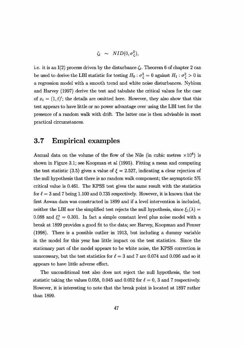
Annual data on the volume of the flow of the Nile (in cubic metres xlO8) is shown in Figure 3.1; see Koopman et al (1995). Fitting a mean and computing the test statistic (3.5) gives a value of £ = 2.527, indicating a clear rejection of the null hypothesis that there is no random walk component; the asymptotic 5% critical value is 0.461. The KPSS test gives the same result with the statistics for i = 3 and 7 being 1.100 and 0.735 respectively. However, it is known that the first Aswan dam was constructed in 1899 and if a level intervention is included, neither the LBI nor the simplified test rejects the null hypothesis, since £i(A) = 0.088 and = 0.301. In fact a simple constant level plus noise model with a break at 1899 provides a good fit to the data; see Harvey, Koopman and Penzer (1998). There is a possible outlier in 1913, but including a dummy variable in the model for this year has little impact on the test statistics. Since the stationary part of the model appears to be white noise, the KPSS correction is unnecessary, but the test statistics for i = 3 and 7 are 0.074 and 0.096 and so it appears to have little adverse effect.

The unconditional test also does not reject the null hypothesis, the test statistic taking the values 0.058, 0.045 and 0.052 for 1 = 0, 3 and 7 respectively. However, it is interesting to note that the break point is located at 1897 rather than 1899.

47

400

300

200

100

000

00

00

00

00

00

1 9 3 0 1 9 5 0 19701 870 1 880 1 89 0 190 0 1 910 1 9 2 0 1 9 4 0 1 9 6 0

Figure 3.1: Volume of the flow of the Nile (cubic metres xlO8)

As a second illustration we apply the tests to annual data on US real GNP for

the period 1909-1970. These data were used in the well-known article by Nelson and Plosser (1982). On the basis of augmented Dickey-Fuller tests, Nelson and Plosser (1982) did not reject the null hypothesis of a unit root. Subsequently, Perron (1989) observed that a structural break is likely to have occured at the

start of the Great Depression, and using his testing procedure he was able to reject the unit root hypothesis in favour of a trend stationary process. Zivot and

Andrews (1992) then modified Perron’s test by endogenizing the breakpoint, but

reached the same conclusion as Perron.

Our own view is that there are a quite a number of places where an argument

can be made for the introduction of a break, or a set of breaks, into an economic time series like GNP. Thus we are not dealing with a situation, as in the case of

the Nile, where there is a well defined event at a particular point in time which one would expect to give rise to a break in the series. Nevertheless, suppose,

following Perron (1989) that we assume there is a known break after 1929 ( that

is t — 1929). Table 3.7a shows the results of applying tests with the KPSS

correction in the following cases: no break, break in the level, and break in

both level and slope. The columns of the table labelled ^=0 to £=8 refer to the

48

LOG(US REAL GNP) TREND6.5

6.25

6

5.75

5.5

5

4.75

L- L1910 1915 1920 1925 1930 1935 1940 1945 1950 1955 1960 1965 1970

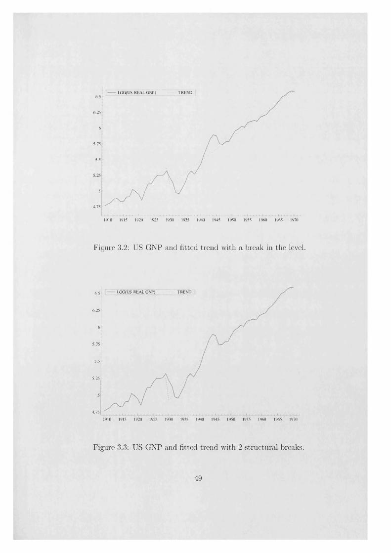
Figure 3.2: US GNP and fitted trend with a break in the level.

IjOG(US REAL GNP) TREND6.5

6.25

5.75

5.5

5.25

4.75

1910 1915 1920 1925 1930 1935 1940 1945 1950 1955 1960 1965 1970

Figure 3.3: US GNP and fitted trend with 2 structural breaks.

49

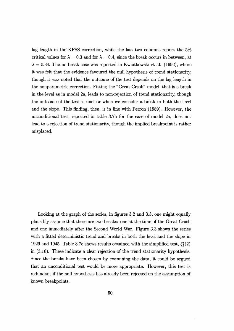
lag length in the KPSS correction, while the last two columns report the 5% critical values for A = 0.3 and for A = 0.4, since the break occurs in between, at A = 0.34. The no break case was reported in Kwiatkowski et al. (1992), where it was felt that the evidence favoured the null hypothesis of trend stationarity, though it was noted that the outcome of the test depends on the lag length in the nonparametric correction. Fitting the ’’Great Crash” model, that is a break in the level as in model 2a, leads to non-rejection of trend stationarity, though the outcome of the test is unclear when we consider a break in both the level and the slope. This finding, then, is in line with Perron (1989). However, the unconditional test, reported in table 3.7b for the case of model 2a, does not lead to a rejection of trend stationarity, though the implied breakpoint is rather misplaced.

Looking at the graph of the series, in figures 3.2 and 3.3, one might equally plausibly assume that there are two breaks: one at the time of the Great Crash and one immediately after the Second World War. Figure 3.3 shows the series with a fitted deterministic trend and breaks in both the level and the slope in 1929 and 1945. Table 3.7c shows results obtained with the simplified test, £5(2) in (3.16). These indicate a clear rejection of the trend stationarity hypothesis. Since the breaks have been chosen by examining the data, it could be argued that an unconditional test would be more appropriate. However, this test is redundant if the null hypothesis has already been rejected on the assumption of known breakpoints.

50

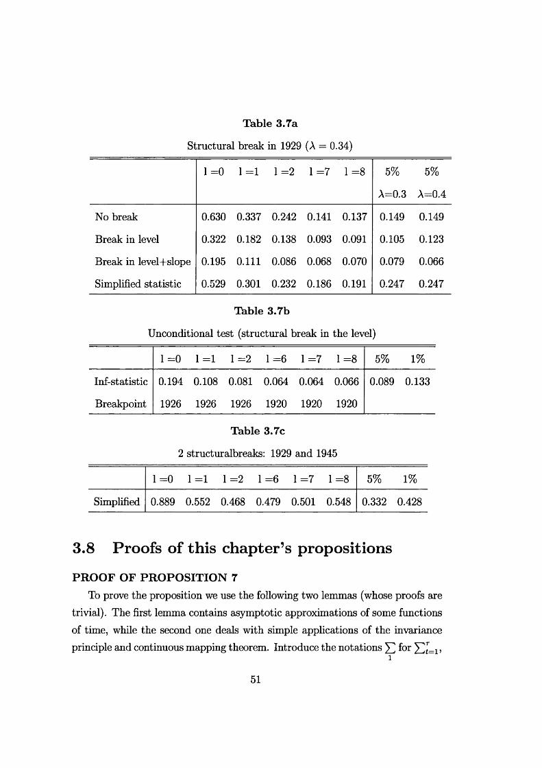
Table 3.7a

Structural break in 1929 (A = 0.34)

1=0 1=1 1=2 1 =7 1 =8 5%

A=0.3

5%

A=0.4

No break 0.630 0.337 0.242 0.141 0.137 0.149 0.149

Break in level 0.322 0.182 0.138 0.093 0.091 0.105 0.123

Break in level+slope 0.195 0.111 0.086 0.068 0.070 0.079 0.066

Simplified statistic 0.529 0.301 0.232 0.186 0.191 0.247 0.247

Table 3.7b

Unconditional test (structural break in the level)

1 =0 1 =1 1 =2 1=6 1=7 1=8 5% 1%

Inf-statistic 0.194 0.108 0.081 0.064 0.064 0.066 0.089 0.133

Breakpoint 1926 1926 1926 1920 1920 1920

Table 3.7c

2 structuralbreaks: 1929 and 1945

00III'­llSOII<MIIHIIoII 5% 1%

Simplified 0.889 0.552 0.468 0.479 0.501 0.548 0.332 0.428

3.8 Proofs o f this chapter’s propositions

PROOF OF PROPOSITION 7To prove the proposition we use the following two lemmas (whose proofs are

trivial). The first lemma contains asymptotic approximations of some functions of time, while the second one deals with simple applications of the invariance principle and continuous mapping theorem. Introduce the notations for Ylt=1»

51

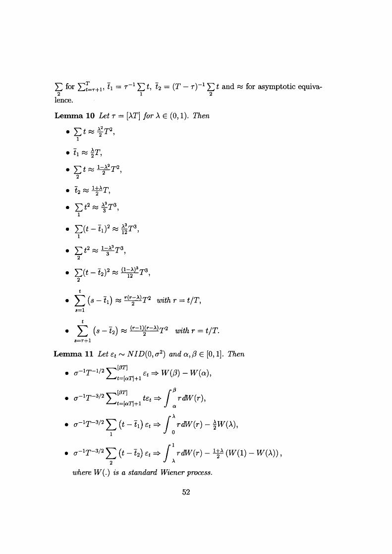
^2 for Ylt=r+v = r 2 = (T — t )~ Y l t and ~ f°r asymptotic equiva-2 1 2

lence.

Lem m a 10 Let r — [XT] for A G (0,1). Then

£ * « # r 2,1

2

*2 « ^ X ,

£ « 2 = s ^ T 3,1

E t t - t l ) 2 * ^ 3,1

£ « 2 « k ^ T 3,2

£ ( t - 12 ) 2 « ^ X 3 ,2

t

5 3 (s - ti) « r f c - ^ r 2 ^ r = t j T 's= 1

t

5 3 (s - *2) « with r = t/T .i—T+1

Lem m a 11 Let et ~ NID(0,cr2) and q , /?€ [0,1]. Then

I*T|+1

S=T+1

V7£)(0,(t2'

a - i r - 1/25 3 ( ’ e, => H/(/3) - W > ),

a 1T 3/2\ ^ tet => [ rdW (r),^ U = [ a T ] + l J a w ’

a - i T - w y ' ( t - t 1) £ t => / rdtV(r) - |W(A), «/ 0

^ - iy - 3/2 5 3 (i - i2) et =!> f 1r dW(r) - Y (W(l) - W(A)),2 J A

where W(.) is a standard Wiener process.

52

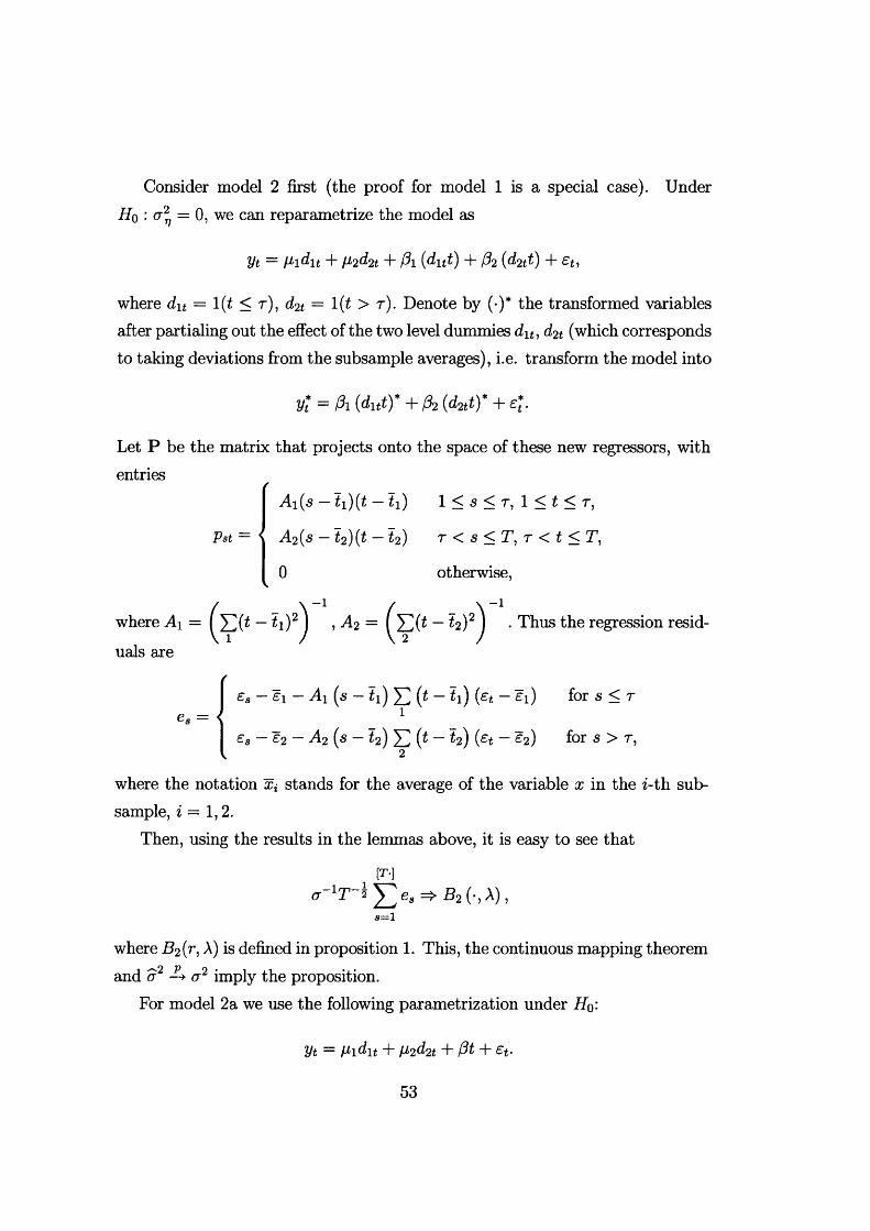
Consider model 2 first (the proof for model 1 is a special case). Under Hq : a2v = 0 , we can reparametrize the model as

Vt — P i d i t + ^ 2^ 21 + A ( d \ t t ) + A ( d 2 t t ) + Et,

where d\t = l(t < r), d2t = 1 (t > t ) . Denote by (•)* the transformed variables after partialing out the effect of the two level dummies du , d2t (which corresponds to taking deviations from the subsample averages), i.e. transform the model into

Vt = A {d\tt)* + A {d>2tt)* + ej.

Let P be the matrix that projects onto the space of these new regressors, with entries f

A\(s — ti)(t — t\) 1 < s < t , 1 < t < r,

Pat = A 2 (s — t2 )(t —1 2 ) r < s < T , t < t < T ,

0 otherwise,

where A\ = ~ ^i)2 » ^2 = — ^ ) 2 • Thus the regression resid­uals are

e , = <

ea - £ i - Ai (s - ti) ^ 2 ( t - ti) (et - £1) for s < r1

e s - e 2 - A 2 ( s - t 2) i f ~ h ) (£t ~ £2) fo r s > t ,

where the notation Xi stands for the average of the variable x in the z-th sub­sample, z = 1, 2.

Then, using the results in the lemmas above, it is easy to see that

[T-]

5=1

where ^ ( r , A) is defined in proposition 1. This, the continuous mapping theorem and d 2 a 2 imply the proposition.

For model 2a we use the following parametrization under H q:

Vt — P i d \ t 4- P2d2t + P t + Et-

53

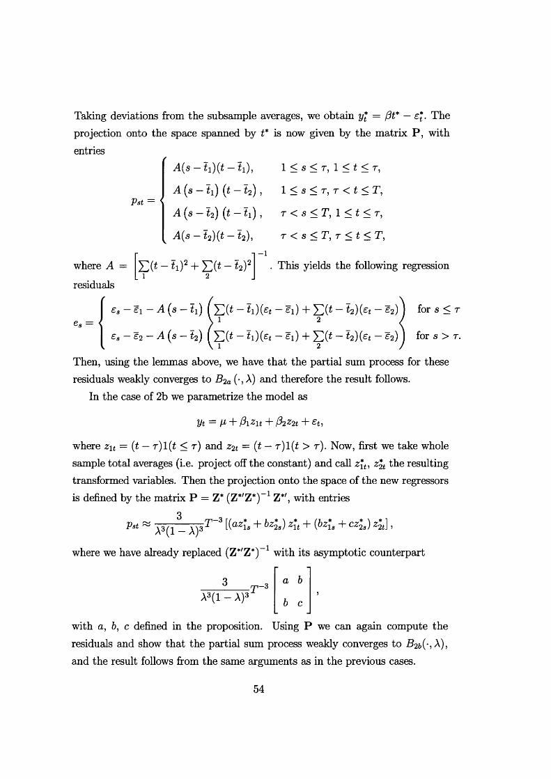
Taking deviations from the subsample averages, we obtain y* = fit* — e*. The projection onto the space spanned by t* is now given by the matrix P , with entries (

A(s — ti)(t — t i ) , l < 5 < r , l < t < r ,

A (s — tfij (t — I2 ) , 1 < s < T, T < t < T,

A (s — £2) (t — ti) , r < s < T, 1 < t < t ,

A(s — t2)(t — ^2 ) , t < s < T , t < t < T ,

Vst =

where A =

residuals

-1. This yields the following regression

e- =ea - e i - A ( s - ti) I - ti)(et - £1 ) + £ (* - t2)(£t - £2 ) ) for s < r

es - £ 2 - A ( s - i 2) ( XX* “ ~ ^1) + £ (^ ~ h ){ e t - e 2) ) for s > r.1 2

Then, using the lemmas above, we have that the partial sum process for these residuals weakly converges to B2a (•, A) and therefore the result follows.

In the case of 2b we parametrize the model as

Vt = V + PiZu + P2z2t + £t,

where z\t — (t — r)l( t < r) and z2t = (t — r) l( t > r). Now, first we take whole sample total averages (i.e. project off the constant) and call z{t , z%t the resulting transformed variables. Then the projection onto the space of the new regressors is defined by the matrix P = Z* (Z*'Z*)-1 Z*', with entries

3Pst T \(az\s + bz*2s) zft + (bzf, + cz*2s) z2*t] ,

A3(l - X)3

where we have already replaced (Z*'Z*)_1 with its asymptotic counterpart

7—3

A3(l — A)3

a b

b c

with a, b, c defined in the proposition. Using P we can again compute the residuals and show that the partial sum process weakly converges to B 2b(- , \ ) ,

and the result follows from the same arguments as in the previous cases.

54

PR O O F OF PR O PO SIT IO N 9Let Ao = tq/ T be the true breakpoint parameter. Consider each of the models

1, 2 , 2a, 2b under the null hypothesis of no random walk and rewrite them as

Vt(Ao) = x't(3+et for t < A0T,(3.26)

yt(A0) = x't(3+w't8+£t for t > A0T,

where for instance for case [2] x t = wt = (1,£)', (3= (/ii,/9i)', 8= (8(jl,8(3). We can also rewrite (3.26) as

where wt( \0) = wt ■ l(t > AoT).When we compute the statistic (3.17) we regress yt(Aq) on xt and wt(A) for

where ^(Aq, A) = wt • l(AoT < t < AT). Therefore we may rewrite (3.27) as

where e*(A, Ao) = £t + (ft{A, Ao)' and zt(A) = (xj, ^(A )')'. The regression (3.30) corresponds to the sequence (over A) of models that we estimate to compute the statistic (3.17).

Let M Z(A) = I - Z(A) (Z(A)'Z(A) ) -1 Z(A)'. The vector of OLS residuals from regression (3.30) is then

2/f(A0) = x'tP + wt(X0)'S+£t, (3.27)

all A. So it is useful to express the true model in terms of wt(A) with A not necessarily equal to Aq. Consider the case A > Ao for example. Then

wt(Ao) = wt W + A), (3.28)

3/i(Ao) — x'tP + wtW S + s t (A, Ao) (3.29)

— +eJ(A,Ao) (3.30)

e(A, A0) — M z (A)e*(A, A0)

= M Z(A) (e + v?(A, A0)5)

= e(A, A) + M z (A)y>(A, X0)S.

(3.31)

(3.32)

(3.33)

55

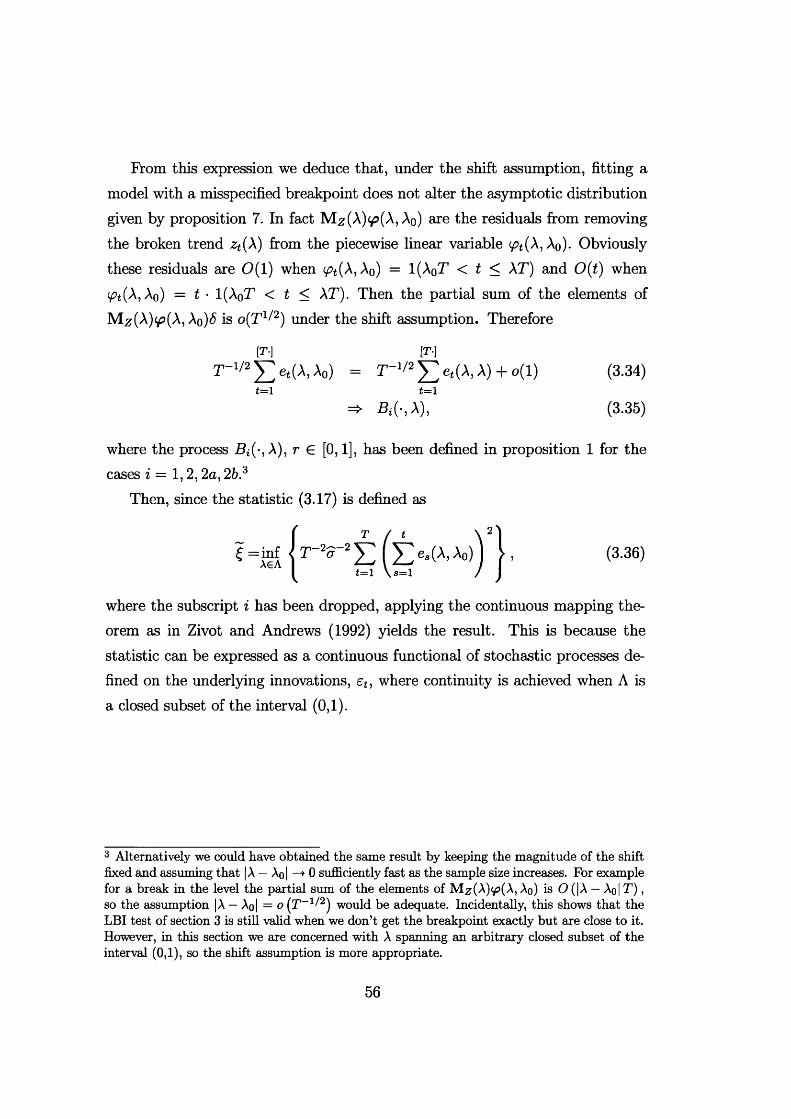
From this expression we deduce that, under the shift assumption, fitting a model with a misspecified breakpoint does not alter the asymptotic distribution given by proposition 7. In fact M ^ (A )y > (A , Ao) are the residuals from removing the broken trend zt{X) from the piecewise linear variable <^*(A, A0). Obviously these residuals are 0(1) when y?t(A, Ao) = l(AoT < t < XT) and 0(t) when

Ao) = t • l(AoT < t < XT). Then the partial sum of the elements of M z (X)cp(X, Xq)S is oiT1/2) under the shift assumption. Therefore

[T-] [T-]

r - 1/2 ^ e t(A,A0) = A,A) + o(l) (3.34)t=1 t=1

=*• (3.35)

where the process £?*(-, A), r G [0,1], has been defined in proposition 1 for the cases i = 1, 2 , 2a, 2b.3

Then, since the statistic (3.17) is defined as

2

£ =inf < AeA t= 1 \s = l

► , (3.36)

where the subscript i has been dropped, applying the continuous mapping the­orem as in Zivot and Andrews (1992) yields the result. This is because the statistic can be expressed as a continuous functional of stochastic processes de­fined on the underlying innovations, etl where continuity is achieved when A is a closed subset of the interval (0 ,1).

3 Alternatively we could have obtained the same result by keeping the magnitude of the shift fixed and assuming that |A — Ao| —» 0 sufficiently fast as the sample size increases. For example for a break in the level the partial sum of the elements of M^(A)y?(A, Ao) is O (|A — Ao| T ) , so the assumption |A — Ao | = o (T-1/2) would be adequate. Incidentally, this shows that the LBI test of section 3 is still valid when we don’t get the breakpoint exactly but are close to it. However, in this section we axe concerned with A spanning an arbitrary closed subset of the interval (0,1), so the shift assumption is more appropriate.

56

Chapter 4

Testing for (com m on) stochastic trends in m ultivariate tim e series

This chapter considers the problem of testing for the presence of stochastic trends in multivariate time series. Here by stochastic trends we mean a multivariate random walk component. If the covariance matrix of the disturbance driving the random walk is not of full rank we have the case of common trends (which also implies cointegration; see chapter 6).

Section 4.1 provides an LBI test on the error covariance matrix in a Gaussian multivariate regression model. This has been obtained by Nyblom and Harvey (2000), hereafter NH, to test for nonstationarity; it can be viewed as a gener­alization of theorem 6 of chapter 2. The asymptotic distributions of the NH test statistic, under both the null and the alternative hypotheses, are derived in section 4.2 for a general specification of the deterministic component which allows for structural breaks as a particular case. Serial correlation in the errors is treated nonparametrically as in section 3.5.1.

The case of structural breaks (sometimes referred to as breaking trends), not considered by Nyblom and Harvey (2000), is examined thoroughly in section 4.3, where critical values for the nonstationarity test are tabulated across a range of values of the breakpoint location parameter. A modified statistic is also proposed whose asymptotic distribution is independent of the breakpoints location and belongs to the Cramer-von Mises family. These results extend those obtained in the previous chapter to a multivariate setting.

Testing for the presence of a certain number of common trends is considered

57

in section 4.4. The asymptotic distribution of the test statistic is derived and critical values axe tabulated for the case of a model with a single breakpoint. This test can also be interpreted as testing the null hypothesis of a certain dimension of the cointegration space against the alternative hypothesis of a smaller dimension.

Tests on the dimension of the cointegration space have been proposed by Jo­hansen (1988, 1991) and Stock and Watson (1988) in the vector autoregression framework. The main difference with respect to our procedure is in the direction of the alternative hypothesis, as their models are ’’more nonstationary” under the null than under the alternative. The Johansen’s type tests have been ex­tended to the case of structural breaks in Kunimoto (1996) and Inoue (1999). Gregory and Hansen (1996a,b) have instead proposed residual based tests for cointegration under regime shifts, but they are not concerned on testing the number of cointegration relationships.

We also show, in section 4.5, that the asymptotic distributions of the test sta­tistics proposed axe unchanged when seasonal dummy variables and/or weakly dependent exogenous regressors axe included in the model. Then, in section 4.6, we illustrate the use of the tests with UK macroeconomic data and data on road casualties in Great Britain. Lastly, section 4.7 contains the proofs of this chapter’s propositions.

4.1 LBI tests on the error covariance m atrix in multivariate regression models

Consider the multivariate Gaussian linear model

Y = XB + E, (4.1)

where Y is a T xN matrix of dependent variables, X is a Txp matrix of fixedregressors, the pxN matrix B contains the regression coefficients, and E is a T x Nmatrix of (zero mean) regression errors. As regards the covariance structure of E, we assume that

Cov(vec( E)) = £ £ <g>f2(0), (4.2)

58

0(0) = D+0H, (4.3)

where E e is a positive definite N x N matrix, D and H are arbitrary known positive definite T x T matrices, and 9 is a non-negative (scalar) parameter.

Note that if D is the identity matrix and H is the random walk generating matrix, then the error term E is the sum of a white noise and a random walk, with the variance of the disturbance term driving the random walk proportional to the variance of the noise. Such model is ’’homogeneous” in the terminology of Harvey (1989, ch. 8).

The interest is in testing Hq : 9 = 0 against H\ : 9 > 0 . The testing problem is invariant under the group of transformation

G = {g : g (Y) = Y P + XA, P nonsingular N x N matrix, A pxN matrix} ,(4.4)

as the conditions of definition 3 of chapter 2 are satisfied.Proceeding in a way analogous to section 2.1.3 it is possible to obtain the

locally most powerful invariant (LBI) test of Ho : 9 = 0 against Hi : 9 > 0. This has been done in Nyblom and Harvey (2000). Here we only report the final result, which is the extension of theorem 6 to a multivariate setting.

T heorem 12 (Multivariate LBI test; Nyblom and Harvey, 2000). For model (4-1)-(4- 3) a locally most powerful test of Ho : 9 = 0 against H\ : 9 > 0 invariant under the group of transformations (4-4) ^

**(Y) =

1 j/tr He'd-1!;) 1 (e'd^hd-'e) j > k,

0 i f t r l ( e 'D ^ e ) _1 ( e 'D - 'H D - 1®) | < k,

where E = (IT- X (X 'X ) -1 X') Y are the OLS residuals from regressing Y on X and k > 0 is an appropriate critical value. Further, the test </>* is also one sided LM test.

In the next section we apply theorem 12 to test for the presence of stochastic trends in a multivariate model, and we derive the distribution of the test statistic under both the null and the alternative hypothesis. The case of serial correlation in the error term is treated nonparametrically as in section 3.5.1.

59

4.2 The distribution o f the test for stochastic trends

Let y t be a vector of N time series. Assume y t is generated by the model (t = l,...,T)

yt = /3'xt+/xt + e t, (4.5)

Mt = P t - i + Vt, (4-6)

Vt ~ *•*•<*•(0,E„), (4.7)

where X* is a p-dimensional vector of nan, — stochastic regressors (including aconstant term), (3 is a px N matrix of parameters, /zf is a multivariate random walk (stochastic trend) with /i0 = 0 , and for the time being et is a white noise disturbance term with Var{et) = S e, independent of rjs for all t and s. When xf = 1 for every t, Harvey (1989) refers to (4.5)-(4.7) as the multivariate local level model.

Under the assumption of Gaussianity, theorem 12 provides the LBI test for H0 : = 0 against Hi : = 0 £ e, 0 > 0. After normalizing by T _1, the testhas a rejection region of the form

tr [S_1C] > k, (4.8)

where C =T~2 Y%=i [E L i et] E L i > S =T _1 E L i etet> et’s ^ the 0LS residuals from regressing y t on x* and k is an appropriate critical value. The test is invariant with respect to the group of transformations y t i— ► P yf + Axt, where P is a nonsingular N x N matrix and A is an arbitrary Nxp matrix.

Under the null hypothesis the model does not contain any stochastic trend component. Under the alternative hypothesis is proportional to i.e. the model is ’’homogeneous” in the sense of Harvey (1989, ch. 8). Thus, the test maximizes the local power against homogeneous alternatives. However the test is also consistent against the more general alternative hypothesis Hi : rank(Yl v) ->0.

NH concentrate on the cases x t = 1 and x t = (1 ,£)', i.e. on the null hypoth­esis of stationarity around respectively a constant level and a linear trend. Here

60

we consider a more general form for the regressors xf, which covers in particular the case of breaking trends.

The case of serial dependence in the disturbance term et can be treated as suggested in section 3.5 relating to the univariate model. In this chapter we only consider the nonparametric correction (or KPSS correction) of the statistic (4.8), which is obtained by replacing S with a consistent estimator of the long run variance of et. The estimator proposed has the form

m

n(rn) = ^ 2 ™(r >m)r(T),T——m

where w (t , m) is a weighting function and

f ( t ) = T - 1 e<eUt—r+1

is the sample autocovariance at lag r. Here we use w (t , m) = 1 — |r |/(m + 1),i.e. the simple Bartlett kernel; other possibilities are examined e.g. in Andrews (1991).

The corrected statistic is then

£n = tr ( O W - 'C ) . (4.9)

The next proposition gives the asymptotic distribution of under the null hypothesis and for an assumption on the regressors x t which includes breaking trends as a particular case. In the next section we will analyze the breaking trends case in detail, providing upper tail percentage points from that distribu­tion.

A ssum ption 4.1. The regressors x t are non-stochastic and there exists a scaling matrix S t and a bounded piecewise continuous function x ( r ) such that (i) StX[tv] —> x ( r ) as T —> oo uniformly in r G [0,1], and (ii) f* x(r)x(r)'dr is positive definite.

A ssum ption 4.2. The vector process {e*} satisfies the following assump­tions: (i) E(ejt) = 0, j = 1 t = 1 ,...,T ; (ii) supfE |^ | 2 < oo, j = 1 ,...,A , (3 > 2 ; (iii) {e*} is strong mixing with mixing coefficients that satisfy

61

2 /S=ia h~2//|S < °°5 Ov) ^ = m ^ ~ 1 (^2 t= i£t Y l ^ i £t>j exists and is positive definite.

A ssum ption 4.3. m —► oo as T —► oo such that m = o (T1/4) .

P roposition 13 Lei yt be generated by the model (4-5)~(4-'7) under assumptions 4-1-4-3. Then under Ho : Yiv = 0

f r r - i [ 1B x (r)'Bx (r)dr, (4.10)Jo

where B x (r) = W(r) — ^ x(r)dW(r)'J (/„ x(r)x(r)'dr) f 'x ( s ) d s , r €[0,1], with W(-) being a standard vector Wiener process of dimension N .

The proof is provided in section 4.7 at the end of the chapter. It extends NH, where only the cases x* = 1 and x* = (1, i)' are considered. In those cases Bx (r) reduces respectively to a standard Brownian bridge, denoted as B ^ r), and to a second level Brownian bridge, denoted as B 2(r), where

B x(r) = W (r) — rW (l), (4.11)

B 2(r) = W (r ) -r W (l) + 6 r ( l - r ) | i W ( l ) - W ( s ) d s ) . (4.12)

More generally, when x t contains all the first h powers of t, i.e. from t° to th~l , B x (r) is a (multivariate) htk-level Brownian bridge as in McNeill (1978) and the distribution of J g B ^ ry B * (r)dr is called hth-level Cramer-von Mises distribu­tion with N degrees of freedom. Percentage points when N = 1 are tabulated in Anderson and Darling (1952), MacNeill (1978), Nyblom and Makelainen (1983), Nyblom (1986), Nabeya and Tanaka (1988), Kwiatkowski et al (1992); when N > 1 percentage points are tabulated in Nyblom (1989), Canova and Hansen (1995), Nyblom and Harvey (2000).

In our case the process Bx (r) is more general as it includes the case of breaking trends for example. We will call this process generalized Brownian bridge.

Assumption 4.1 follows Phillips and Xiao (1998). Note that it excludes the dummy variables used to model seasonal effects; however in section 4.5 we will

62

show that adding these dummies does not affect the limiting distribution. As­sumption 4.2 permits a fairly general correlation structure for the disturbances et, which can also be heteroscedastic. Assumption 4.2 is sufficient for applying the invariance principle and, together with assumption 4.3, for the consistency of fi(m); see Phillips (1987). Note that imposing stronger conditions on et would allow faster rates for m. For example, in the classical spectral theory of station­ary process only m = o(T) is required. In practice the rate m = o{T1/2) can be satisfactory under both the null and the alternative hypothesis; see Kwiatowski et al. (1992).

The percentage points from the distribution of (4.10) can be used to construct an asymptotically valid test for the null hypothesis of Hq : = 0 againstH\ : ranA;(Sr?) > 0. If et is a white noise process, then the test is asymptotically equivalent to the LBI test (4.8).

Under the alternative hypothesis H\ : rank(Jj,,) = K > Othe statistic di­verges, so the test is consistent. The asymptotic distribution of (m /T ) fjv under H\ is established by the following proposition.

Proposition 14 Let yt be generated by the model (4-5)~(4-7) under assumptions4.1-4-3. Then under Hi : ranfc(S^) = K > 0

- i tr j QT W x (s)W x (s)'ds) Q f W x (s)ds) ( j ( W x (s)ds) dr

where W x (r) = W (r) — W (r)x(r)'dr (Jo1 x(r)x(r)'dr^ x(r), r G [0 , 1], with W(-) being a standard vector Wiener process of dimension K.

The proof is provided in section 4.7 at the end of the chapter. The process W x (-) is the projection in L2 [0 , 1] of a Wiener process onto the space or­thogonal to the span of x(-). For x t = 1 it becomes the ”demeaned Wiener process” W (r) — f* W(r)dr, and for x t — (1, t)' it becomes the ”detrended Wiener process” W (r) + (6r — 4) Jq W ( r)dr — (12r — 6) rW(r)dr.

The NH test, based on the statistic (4.8)/(4.9) with x t = 1 or x t = (1 ,£)', is also consistent against the alternative hypothesis of a shift in the deterministic

63

trend. This follows from the same arguments examined in the previous chapter (relating to the univariate version of this model), see also Gardner (1969), Ny­blom (1989), Lee et al. (1997). In the next section we therefore study the case of breaking trends when testing for the presence of a random walk component in a multivariate model. The results collapse to those obtained in the previous chapter when the number of the series N is one.

4.3 Testing in the presence o f structural breaks

Suppose that there is a shift in the deterministic trend of the series at time T\ = XT, X € (0,1). We assume that the breakpoint A is exogenous and known. Like in the previous chapter, we consider the model (4.5)-(4.7) under four different specifications of the deterministic trend. Let

(l,w t(A))' i = 1,

( l , t ,w t(X),twt(X))' i = 2,

( l , t ,w t(X))' i = 2a,

(1, t, (t - XT)wt(X))' i = 2b,

(4.13)

where wt(X) = 1 (t > XT) . Case 1 corresponds to a level break with no slope, case 2 to a structural break in both the level and the slope, whereas in case 2a and 2b the break occurs respectively in the level only and in the slope only.

Since <5 xJTrj(A) —► x*(r; A), defined by

x\ r > A) = <

( l ^ r j A ) ) ' i = 1,

(l,r,w(r; X),rw{r\A))' i = 2,

(1 ,r,w(r-,X))' i = 2a,

k ( l , r , ( r - X)w(r;X))' i = 2b,

(4.14)

with w(r; A) = l( r > A), assumption 4.1 holds. Therefore we can apply propo­sition 13. Call fJy(A) the statistic (4.9) constructed using xJ(A) as regressors,

64

i = 1,2,2a, 26. Then under Hq

&(A) - i / B*(r; A)'B1(r; A)*-, (4.15)Jo

where the definition of the generalized Brownian bridge B*(r; A) is obtained by proposition 7 after replacing the underlying scalar Wiener process with a TV-dimensional one.

The upper tail percentage points for the distribution of (4.15) when A = 0.002, 0.1, 0.2, 0.3, 0.4, 0.5 are reported in the first column (labelled K = 0) of tables 4.1, 4.2, 4.2a, 4.2b. The values for A > 0.5 are not reported since the distribution is symmetric around A = 0.5. These percentiles are obtained by simulating the processes B*(r; A), i = 1,2 , 2a, 26, using a sample size of 1,000

and 100,000 replications. We use the random number generator of the matrix programming language Ox; see Doomik (1998). Note that the values for A = 0.002 closely agree with the values reported in Nyblom and Harvey (2000), which refer to the case A = 0 and were obtained using the series expansion of the distribution.

The statistic Q^(A) can then be used to construct an asymptotically valid test for the presence of stochastic trends for multivariate time series with structural breaks, using the first column of tables 4.1-4.2b to select the appropriate critical values.

The test based on Qv(A) has desirable properties, among which being as­ymptotically equivalent to the LBI test for a Gaussian model with serially in­dependent disturbances. However the critical values depends on the breakpoint parameter A.

In the following subsection we then propose a modified version of the statistic Qv(A) for which the asymptotic distribution is independent of A. This extends to multiple breakpoints and allows us to tabulate critical values across multiple dimensions of the breakpoint location. The following subsection also extends the results of section 3.3 to a multivariate setting.

65

(3 345 6 464 6 746

-Q M S 0351 ------- 0 6 2 2 ■0553----- 0l20----- 5152]

- - - - - — -0 062 o o T s O U T]T557------ i"255-----1575

-0 5 4 7 -------0 056------- 00841T 2 7 3 -------146 5------- rsT T ■■■■■■” ■■■■■■ 0.240 0.289 0.431

-0 0 8 4 -------5 0 9 7 ------- 0 1 3 3 0.037 0.044 0.062

Figure 4.1: TABLE 4.1

6 ~ 5 ~ 5 14T 0 817

T 5 8 4 ------- 0 l0 5 -------0 1 5 5

: 0 075

-0376 -------0 422-------0 521 -0 0 4 6 -------0 0 5 6 -------00821

0-455-------0 3 0 4 -------0 6 1 3 ■ -V.- - -Vf -- ---rV. - .. - . , -0 0 3 6 -------0 0 4 3 -------00621

Figure 4.2: TABLE 4.2

66

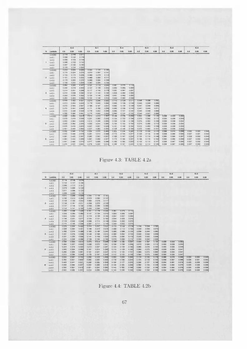
" ■ 0 084 0 105 0 160

lo g i 0 0 7 5 -------5173■0394-----5135-----5737

■5175-----o!33-----513T r --- -0 046-----oo5e 55531

■5174-----53T3-----5157 T _ " ■ -0 083-----5096-----5135

0 202 0 228 0 293 0 0 3 0 0 0 3 5 0 0 4 8■5533-----5555-----5755 ■5134-----5175-----5155

Figure 4.3: TABLE 4.2a

wmmrm Tm

■ 0 084 0 106 0 160

-5355-----5135-----5135 "5151----- 5175-----5345 155i----- 5175-----5TT3

■■" H i! 5347-----5133 1 0 4 6 5156 5153

- ~~ 1154-----5157-----5135

--- - -

Figure 4.4: TABLE 4.2b

67

4.3.1 A modified statistic

Here we restrict our attention to the cases i = 1 and i = 2 of the deterministic component x{(A) in (4.13). Denote by eJ(A) the residuals from the OLS regression of on xJ(A), i = 1,2 . Note that the orthogonality conditions for the residuals allow us to write ( i = 1, 2)

£ ( £ ^ ( A ) ) ( t et(A))' =

= E ( i > U A ) ) (x>*(A)Y+ ± ( ± 4(A)) ( ± 4(A))',t=1 \ s = l / \ S =1 / t=Ti+l \s=Ti+l / \a=Ti+l /

as the sum of residuals in each of the two subsamples {l,...,Ti} and {Ti + 1, T } is zero. The idea is then essentially to take the sum of the two statistics (4.9) applied to each subsample. In particular, we consider the statistic £$(A) defined as

$(A ) = t r [ f i ( m ) - 1 (C^A) + C2(A))] , i = 1,2, (4.16)

where

c 1(A) = r 1- 2 E f E eUA)) ( E ' W ) >t —1 \ s = l / \s = l /

C2(A) = ( T - Ti ) - 2 E f E e*(A)) f E e»(A)t = T i + l \«=Ti+l / \ s = T i+1

and f2(m) defined as in section 4.2.

P roposition 15 Let yt be generated by the model (4-5)-(4-7) under assumptions 4-2-4-3 and with the regressors defined by (4-13). Then under Ho i 'Ejj = 0

$ (A ) 4 f B <(r)'B‘(r)dr, * = 1,2, (4.17)J 0

where B x(r) and B 2(r) are respectively a standard vector Brownian bridge and a second level standard vector Brownian bridge of dimension 2N.

The proof is in contained in section 4.7 at the end of the chapter. The random variable to which (A) converge has then a Cramer-von Mises distribution with

68

2N degrees of freedom. As said before, percentage points from this distribution are tabulated in Nyblom (1989), Canova and Hansen (1995), Nyblom and Harvey (2000), and also reported in table 3.2 of the previous chapter. They can be used to construct an alternative test for Ho : = 0 against Hi : ranki^l^) > 0

in a model with breaking trends. This test coincides with the LBI test (4.15) when A = 0.5, since £JJ(0.5) = 0.25^(0.5).1 For other values of A the test is of course consistent; furthermore the simulation results in section 3.3, relating to the univariate version of the test, show that it suffers only a small loss in power compared with the LBI test.

The attraction of the test (4.16) is that it can be easily generalized to the case of two or more breaks in the deterministic trend. Let there be two structural breaks at time T\ = \ \ T and T2 = A2T. Then we can base the test for the presence of stochastic trends on the statistic

$ (A i, A2) = tr [fJ(m) - 1 (C 1 , A2) + C 2(AI,A2)+ C 3(A1,A2))] , t = 1,2,

which will be defined by generalizing (4.16) in an obvious way. Its asymptotic distribution is Cramer-von Mises with 3N degrees of freedom.

Another case can be covered by the statistic f)J(Ai, A2), namely when some of the N series break at the point Ai and some at the point A2. Then constructing the statistic by forcing all the N series to have two breakpoints gives rise to a valid test, although not efficient. On the other hand, for this situation no alternative procedures seem available in the literature.

4.4 Testing for common trends

In this section we consider the model (4.5)-(4.7) under the null hypothesis H0 : rank(Sjv) = K , with 0 < K < N, which corresponds to nonstationarity with K stochastic trends. The alternative hypothesis is Hi : rank(S „ )> K .

The existence of K common trends implies the existence of R = N — Kcointegration relationships, i.e. there is a R xN (full rank) matrix A such that1 From the results in section 4.7 (see also section 3.3) it follows that for i — 1,2 the asymptotic distribution of £%N (A) can be also represented as the distribution of a weighted sum of twoCramer-von Mises random variables with N degrees of freedom, with weights given by A2 and( 1 - A ) 2.

69

Ay* is stationary. If we knew A, we could test H q against H \ by applying the statistic (4.9) to Ay*. But since A is unknown, one way of proceeding is to take the minimum of (4.9) over the set of the R xN matrices A. The minimum isgiven by the sum of the R smallest eigenvalues of fi(ra)_1C; see Rao (1973) andNyblom and Harvey (2000).

The statistic we use is thenN

£k , n = 5 ^ (4 -18)j = K +1

where ^ i > ^ 2 > - - - > ^ j v > 0 are the N ordered eigenvalues of fi(m )- 1C. Note that fo,AT corresponds to the statistic (4.9).

P roposition 16 Let yt be generated by the model (4-5)-(4-7) under assumptions4.1-4.3. Then under Ho : ranfc(ST?) = K

£k,n - i tr (C-22 - C l 'C I r 'c y , (4.19)

where the stochastic matrices C*j, i , j = 1, 2 , are defined as

C'n := jT f f i w x (s)d.s\ Bx (r)’dr,

C i, := [ B x (r)Bx (r)'dr, Jo

where W x (r) is a K-dimensional vector process as defined in proposition 1 4 a,nd Bx (r) is a R-dimensional vector process as defined in proposition 13.

The proof is in section 4.7 at the end of the chapter. Under Hi : rank(Ti v) > K , the statistic £k ,n diverges to infinity as it contains at least one eigenvalue that is Op(T/m); see section 4.7.

For the case of breaking trends, i.e. when the regressors are defined by (4.13), the upper tail percentage points of the distribution of £k,n under H q are provided in Tables 4.1, 4.2, 4.2a, 4.2b for a range of values of the breakpoint parameter A. These are obtained simulating the stochastic processes involved using a sample size of 1,000 and 100,000 replications.

70

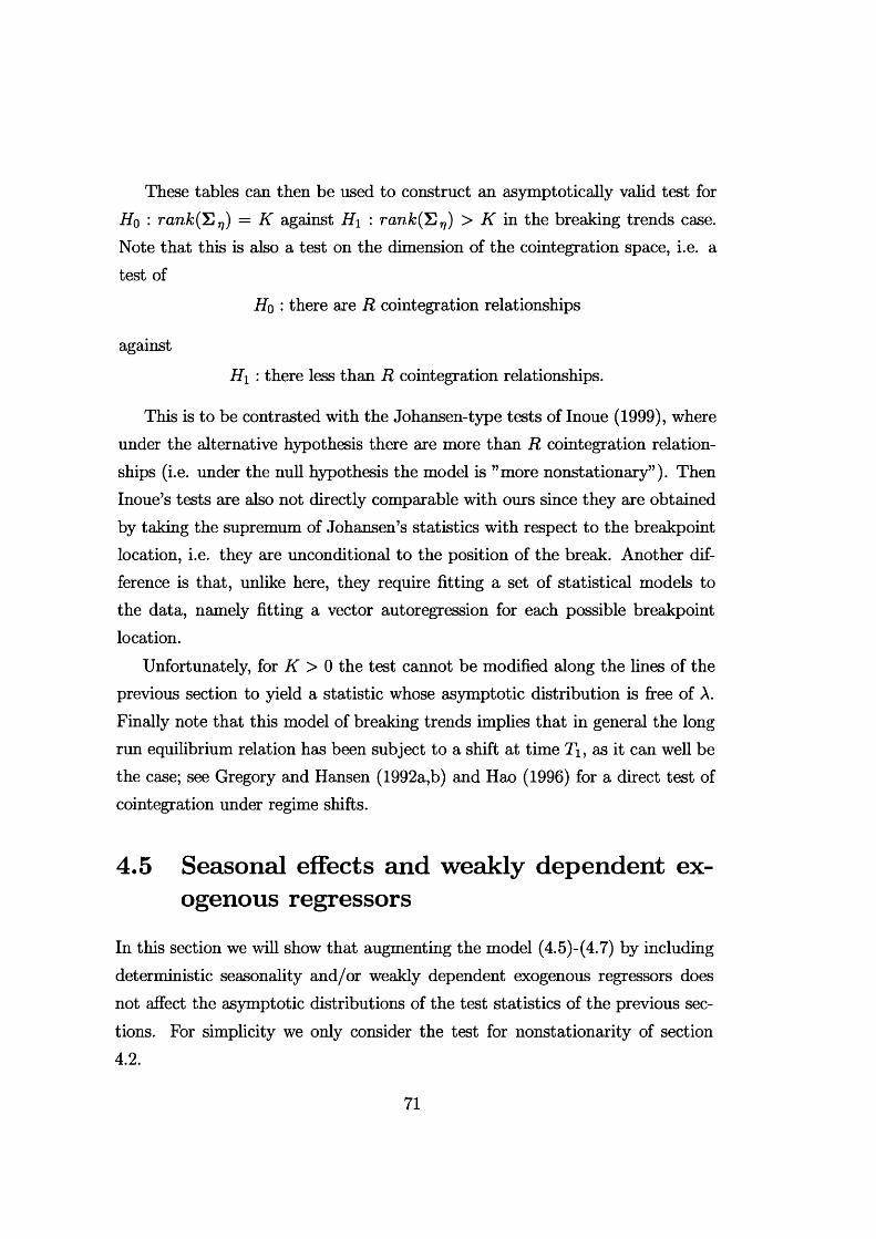
These tables can then be used to construct an asymptotically valid test for H q . r a n k e r ) ) — K against H\ . TQ/n,k(^Oi 77) > K in the breaking trends case. Note that this is also a test on the dimension of the cointegration space, i.e. a test of

H q : there are R cointegration relationships

against

Hi : there less than R cointegration relationships.

This is to be contrasted with the Johansen-type tests of Inoue (1999), where under the alternative hypothesis there are more than R cointegration relation­ships (i.e. under the null hypothesis the model is ’’more nonstationary”). Then Inoue’s tests are also not directly comparable with ours since they are obtained by taking the supremum of Johansen’s statistics with respect to the breakpoint location, i.e. they are unconditional to the position of the break. Another dif­ference is that, unlike here, they require fitting a set of statistical models to the data, namely fitting a vector autoregression for each possible breakpoint location.

Unfortunately, for K > 0 the test cannot be modified along the lines of the previous section to yield a statistic whose asymptotic distribution is free of A. Finally note that this model of breaking trends implies that in general the long run equilibrium relation has been subject to a shift at time Ti, as it can well be the case; see Gregory and Hansen (1992a,b) and Hao (1996) for a direct test of cointegration under regime shifts.

4.5 Seasonal effects and weakly dependent ex­ogenous regressors

In this section we will show that augmenting the model (4.5)-(4.7) by including deterministic seasonality and/or weakly dependent exogenous regressors does not affect the asymptotic distributions of the test statistics of the previous sec­tions. For simplicity we only consider the test for nonstationarity of section 4.2.

71

Replace equation (4.5) by

y t = (3'xt+'y,z t + fj,t + eu (4.20)

where z t are additional regressors and 7 the corresponding coefficients.

A ssum ption 4.4. Either [A] or [B] below holds.

[A] z t is a zero mean second order stationary process such that:

IA11 E £ i l|E(ztzi)|| < OO, [A2] E(zteJ) = 0,[A3] l im T ^ E ^ ^ j z,eit) (E L i z,eit) < oo, i = 1 , N .

[B] z t = (zit, is a set of s — 1 deterministic seasonal dummy vari­ables, defined by

/

1 t = h + nS,

Zht = 0 t ^ h + ns , (4-21)

—1 t = ns ,

for 7?- = 0 ,1 ,2 ,... Furthermore the function x(r) of assumption 4.1 is of bounded variation, i.e. there exists M < oo such that for every finite partition of the unit

interval 0 = r0 < n < ... < rn = 1, YJU\ llx (r 0 - x (r i-i)ll <

In assumption 4.4[A] zt is a weakly dependent process (in second order sense) since 4.4[A1] implies a finite spectrum at the origin. 4[A2] is an exogeneity condition. The zero mean assumption is innocuous since an intercept is included among the other regressors x t.

The seasonal dummies of assumption 4[B] sum to zero over s periods, so they represent the relative seasonal deviation from the common mean. A reparame- trization of the seasonal effect could be used. The bounded variation condition is of course satisfied in the breaking trends case.

Let the statistic of section 4.2, equation (4.9), be constructed using theresiduals from regressing y t on (x J, z't)'. Then the following proposition holds.

P roposition 17 Let yt be generated by the model (4-20),(4-6)-(4-7) under as­sumptions 4-1-4-4- Then, under H0 : = 0, the asymptotic distribution of£xis the one defined in proposition 13.

72

The proof is in section 4.7 at the end of the chapter. Proposition 17 implies that we can use the tests of sections 4.2, 4.3 to test for the presence of stochastic trends also in models containing a deterministic seasonal component and/or weakly dependent regressors. The same result carries over to the common trend test of section 4.4. The proof is not provided but follows similar lines.

When the seasonality is stochastic and possibly there are seasonal unit roots, the strategy advocated by Harvey and Streibel (1997) can be applied. The idea is described in section 3.5.2 as a way to account for serial correlation in et , but it can be extended to deal with stochastic seasonality (by introducing it in the state space model to be estimated).

The case of 1(1) regressors z t is examined in Choi and Ahn (1995). They consider testing for stationarity of the errors in multiple equations with inte­grated variables. In their framework stationarity of the errors corresponds to cointegration between regressands and regressors.

4.6 Examples

The use of the tests is illustrated with two examples, one using UK macroeco­nomic data and the other using data on road casualties in Great Britain. The last dataset was used by Harvey and Durbin (1986) to study the effect of the introduction of the seat belt law and is provided with the program STAMP 5.0 of Koopman et al. (1995).

Figures 4.5-4.7 plot the logarithms of UK gross domestic product, consump­tion and investment for the period 1960-1990, together with a fitted deterministic trend. The data are quarterly, seasonal adjusted and at constant 1990 prices. The source is the Central Statistical Office.

We have assumed that there was an exogenous structural break around 1979- 1980; the plot of the series, the investment in particular, seems to sustain the assumption. The exogeneity of the break may be due to the following two reasons: first the second oil shock of 1979-1980 may have caused a drop in the series and secondly 1979 coincides with the election of a right wing government with Margaret Thatcher as Prime Minister which may have determined the

73

/

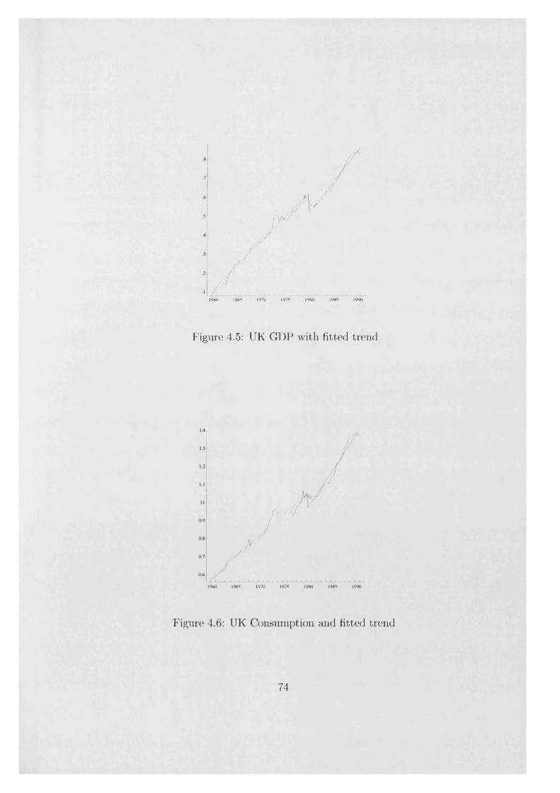
/w

jyxr

v/

<r..................................I960 1965 I‘>70 1‘>7S 1980 1985 1990

Figure 4.5: UK GDP with fitted trend

,v ,V

,A '

,I960 1965 1970 1975 1980 1985 1990

Figure 4.6: UK Consumption and fitted trend

74

0.3

0.2

0.1

10

9.9

9.8

9.7

9.6

9.5

9.4

9.3

Figure 4.7: UK Investment and fitted trend

higher growth rates of investment thereafter. Thus we have chosen to fit a broken linear trend to the data, with the break occurring in the second quarter

of 1980.2We consider the case of a break in both level and slope and we apply the

common trend test of section 4.4 to the trivariate series of (log) gdp, consumption

and investment. The results are displayed in table 4.3, for various values of

the lag length parameter m. The breakpoint is at the second quarter of 1980,

corresponding to a value for A of 0.66. Note that the statistic for K = 0 is equivalent to the nonstationarity test statistic of section 4.3, case 2. The critical values for the case of no break are taken from Nyblom and Harvey (2000), those

for the case of structural break are taken from table 4.2, N=3 and A=0.3.

From standard macroeconomic arguments, we would expect the existence of

one stochastic trend among the variables, probably representing the effect of

technological progress. However table 4.3 shows that the null hypothesis of one

common trend (K = 1) is rejected at 5% significance level when we don’t take

into account the structural break of 1979-1980. Indeed, even the hypothesis of

two trends seems to be rejected. On the contrary, fitting a broken deterministic

2 Of course there might have been other events that, on a priori grounds, could have deter­mined a break in the series. However, since the purpose of this section is only to illustrate the use of the tests, we don’t go deep into the issue of exogeneity of the breakpoint.

1965 1970I960

75

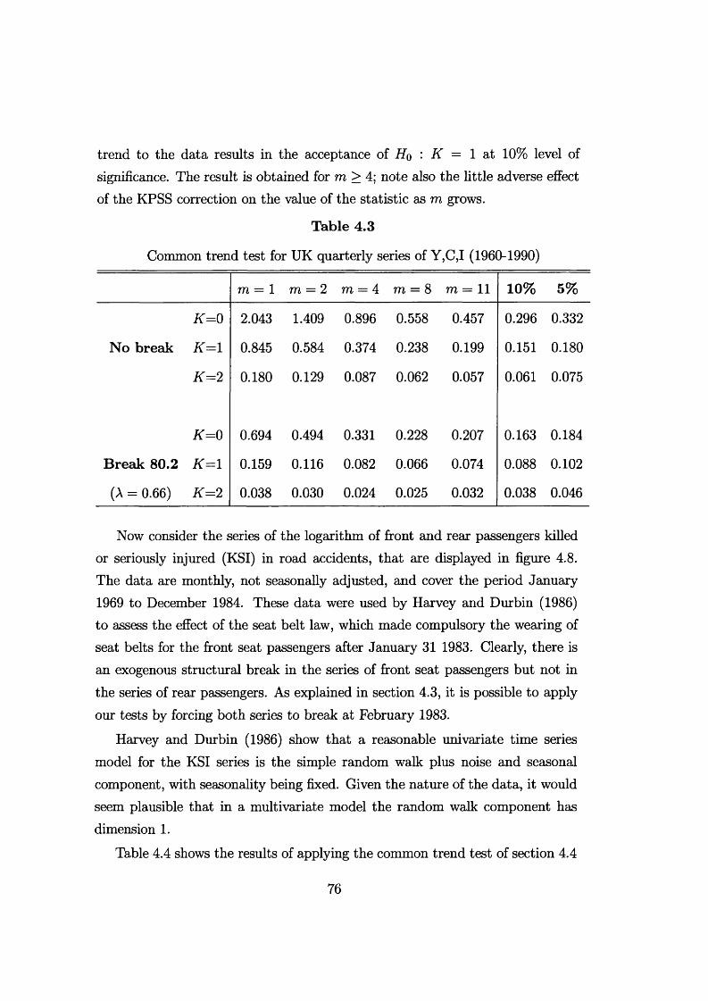
trend to the data results in the acceptance of Hq : K = 1 at 10% level of significance. The result is obtained for m > 4; note also the little adverse effect of the KPSS correction on the value of the statistic as m grows.

Table 4.3

Common trend test for UK quarterly series of Y,C,I (1960-1990)

771= 1 m = 2 771 = 4 771 = 8 771 = 11 1 0 % 5%

K = 0 2.043 1.409 0.896 0.558 0.457 0.296 0.332

No break K = 1 0.845 0.584 0.374 0.238 0.199 0.151 0.180

K = 2 0.180 0.129 0.087 0.062 0.057 0.061 0.075

K = 0 0.694 0.494 0.331 0.228 0.207 0.163 0.184

B reak 80.2 K = 1 0.159 0.116 0.082 0.066 0.074 0.088 0.102

(A = 0.66) K = 2 0.038 0.030 0.024 0.025 0.032 0.038 0.046

Now consider the series of the logarithm of front and rear passengers killed or seriously injured (KSI) in road accidents, that are displayed in figure 4.8. The data are monthly, not seasonally adjusted, and cover the period January 1969 to December 1984. These data were used by Harvey and Durbin (1986) to assess the effect of the seat belt law, which made compulsory the wearing of seat belts for the front seat passengers after January 31 1983. Clearly, there is an exogenous structural break in the series of front seat passengers but not in the series of rear passengers. As explained in section 4.3, it is possible to apply our tests by forcing both series to break at February 1983.

Harvey and Durbin (1986) show that a reasonable univariate time series model for the KSI series is the simple random walk plus noise and seasonal component, with seasonality being fixed. Given the nature of the data, it would seem plausible that in a multivariate model the random walk component has dimension 1.

Table 4.4 shows the results of applying the common trend test of section 4.4

76

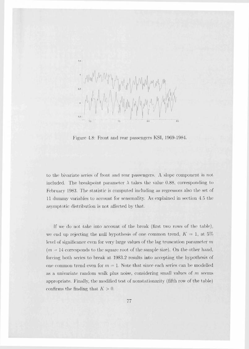
Figure 4.8: Front and rear passengers KSI, 1969-1984.

to the bivariate series of front and rear passengers. A slope component is not included. The breakpoint parameter A takes the value 0.88, corresponding to

February 1983. The statistic is computed including as regressors also the set of 11 dummy variables to account for seasonality. As explained in section 4.5 the

asymptotic distribution is not affected by that.

If we do not take into account of the break (first two rows of the table),

we end up rejecting the null hypothesis of one common trend, K = 1, at 5%

level of significance even for very large values of the lag truncation parameter m (ra = 14 corresponds to the square root of the sample size). On the other hand,

forcing both series to break at 1983.2 results into accepting the hypothesis of

one common trend even for m = 1. Note that since each series can be modelled

as a univariate random walk plus noise, considering small values of m seems

appropriate. Finally, the modified test of nonstationarity (fifth row of the table) confirms the finding that K > 0.

77

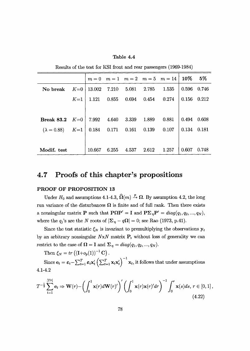
Table 4.4

Results of the test for KSI front and rear passengers (1969-1984)

m = 0 m = 1 m = 2 m = 5 m — 14 1 0 % 5%

No break K = 0

K = 1

13.002

1.121

7.210

0.855

5.081

0.694

2.785

0.454

1.535

0.274

0.596

0.156

0.746

0.212

B reak 83.2

(A = 0.88)

K = 0

K = 1

7.992

0.184

4.640

0.171

3.339

0.161

1.889

0.139

0.881

0.107

0.494

0.134

0.608

0.181

M odif. tes t 10.667 6.255 4.537 2.612 1.257 0.607 0.748

4.7 Proofs of this chapter’s propositions

PR O O F OF PR O PO SIT IO N 13Under H0 and assumptions 4.1-4.3, fi(ra) fl. By assumption 4.2, the long

run variance of the disturbances is finite and of full rank. Then there exists a nonsingular matrix P such that P U P ' = I and P E ^ P ' = diag(qi,q2, ...,<jjv), where the q^s are the N roots of IS^ — qfl\ = 0 ; see Rao (1973, p.41).

Since the test statistic £/v is invariant to premultiplying the observations y t by an arbitrary nonsingular N xN matrix P, without loss of generality we can restrict to the case of O = I and = diag(qi, q2 , - ‘, 9jv)-

Then £N = tr ((I+op(l)) 1C ) .

xt , it follows that under assumptions

(4.22)

78

where W (r) is a standard vector Wiener process of dimension N. We denote the process at the right hand side of (4.22) as B x (r), and we call it generalized Brownian bridge. Thus, by the continuous mapping theorem and using the definition of C, £/v Jq B x (r)'Bx (r)dr.

PR O O F OF PR O PO SIT IO N 14Let assumptions 4.1-4.3 hold. Without loss of generality we again restrict to

the case of f l = I and = diag(qi, ..., q^). The hypothesis Hi : ra n ker ,) = K can be equivalently formulated as H\ : qj > 0 for j = 1, K and qj = 0 for j = K + l,...,N .

Consider the OLS residuals for the j -equation under Hi,

(t \ —1 T

X XtX*J j =t=i / t=i

and/ T \ _1 T

ejt = £jt ~ xi I 5ZXtX't I H Xt£J*’ j = K +\t=i ) t=l

since jijt = 0 for j = K + 1,..., N , t = 1, ...,T.Then, the following weak convergence results hold:

T - 1/ 2e U Tr] =»• QiWfir), j = 1, •••, K, (4.23)[TV]

r ~3/2 Z e* =►t=1 [!Tr]

T ~1/2'5 2 eit =*• j = (4.25)t=l

where the processes W *(r) and B x (r), r € [0,1], are the one-dimensional ver­sion of the processes defined in the statements of proposition 14 and 13, and are uncorrelated across j (and with each other). The results (4.23)-(4.25) are obtained applying the invariance principle to the partial sums of et and rjt and using assumption 4.1 of non-stochastic regressors.

Denote by Cjh, u)jh the (j, h)-elements of the matrices C, Q(m). Then we have the following further asymptotic results:

/JoW x (s)ds, j = 1,..., K, (4.24)

79

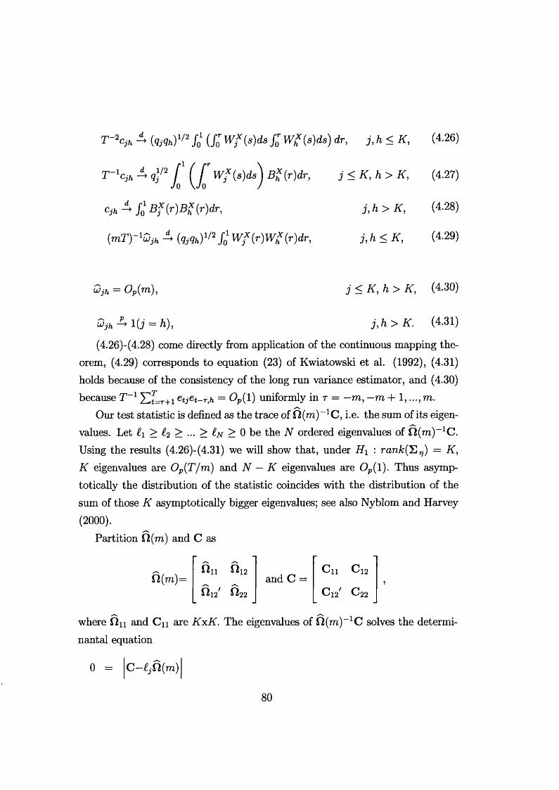
T-\k - i f e < f c ) 1 /2 / o (fo Wf(s)dsj; Wf(s)ds) dr, j, h < K, (4.26)

T 1clh - i q1/ 2 J (J W f (s)ds \ B * (r)dr, j < K , h > K , (4-27)

cih fo Bf(r)B%(r)dr, j, h > K, (4.28)

(mT)~lWjh - i fe9fc)1/2/o Wf(r)Wj?(r)dr, j , h < K, (4.29)

= Op(m), j < K, h > K, (4.30)

U = h), j, h > K. (4.31)

(4.26)-(4.28) come directly from application of the continuous mapping the­orem, (4.29) corresponds to equation (23) of Kwiatowski et al. (1992), (4.31) holds because of the consistency of the long rim variance estimator, and (4.30) because T~l Ylt=T+1 e t j e t - r , h = Op( 1) uniformly in r = —m, —m + 1,..., m.

Our test statistic is defined as the trace of n(m )~ 1C, i.e. the sum of its eigen­values. Let i\ > t<2, > ... > £n > 0 be the N ordered eigenvalues of n (m )_1C. Using the results (4.26)-(4.31) we will show that, under Hi : rank{'X^) = K, K eigenvalues are Op(T/m) and N — K eigenvalues are Op( 1). Thus asymp­totically the distribution of the statistic coincides with the distribution of the sum of those K asymptotically bigger eigenvalues; see also Nyblom and Harvey (2000).

Partition H(m) and C as

fi(ra)=

where Qn and C n are KxK. The eigenvalues of fi(m) C solves the determi- nantal equation

fin-As

f il2 C n C 12and C =

fi 12 1 22 C i2' C 22

0 = C —£ j Q ( m )

80

Cn — i j f l n

x C 2 2 — 22 — ^ C i 2 — ^ - ^ 1 2 ^ ( C n — C jQ u ) ^ C i 2 —

see Rao (1973, p.32). Then using (4.26)-(4.31) we see that the roots of the first determinant are Op(T/m ), whereas the roots of the second determinant are

with W x (r) being the If-dimensional vector process defined in the statement of the proposition.

PROOF OF PROPOSITION 15Let z t = 1 for the case i = 1 and z t = (1 ,£)' for the case i = 2, and drop

the superscript i for simplicity. The model can be equivalently parametrized using as regressors xt(A) = (xn(A)',x2f(A)/) ' , where xit(A) = zt • 1 (t < AT), x2t = z t ■ 1 (t > X T) . Then the model is orthogonal and to obtain the OLS residuals we can consider the two subsamples {l,...,Ti},{Ti + 1 , T} separately and in each of them regress y t on zt.

Again, without loss of generality and under assumption 4.2, we can restrict to the case of O = I and = diag(qi,q2 , Then, under assumptions4.2-4.3, we can write £}J(A) = tr [(I + op( 1)) 1 (CX(A) + C 2(A))] . Under Hq the

Op( 1) and asymptotically equivalent to the eigenvalues of (C22 — C'12C 111C i2); see Nyblom and Harvey (2000) for further details.

Therefore (m / T ) —► tr 1CJ1) , where

invariance principle can be applied in each subsample, yielding

[T i r \

r r 1/2 E ei(A)= * B‘i(r )-t=1

t=1

81

where B^(r), B ^ r) axe TV-dimensional independent standard vector Brownian bridges for i = 1 and second level Brownian bridges for i = 2. Independence holds because the two Brownian bridges are the limit of partial sum processes containing non-overlapping subsets of disturbances.

By the continuous mapping theorem it then follows that £)J(A) converges to the sum of two independent random variables, each with a Cramer-von Mises dis­tribution with TV degrees of freedom. The limiting distribution is then Cramer- von Mises with 2TV degrees of freedom; see section 3.3 for details on the additivity property of Cramer-von Mises random variables.

PROOF OF PROPOSITION 16From the proof of proposition 14 we know that under assumptions 4.1-4.3 and

under rank(Yin) = K , the R smallest eigenvalues of H_1C are asymptotically equivalent to the eigenvalues of C 22 — C i2/C n _1C i2. Then, using the results(4.26)-(4.28),

T~2C n - i QSC^Q*,

r - 'C j s - i Q 5 c ;2lC d p*

22 > ^ 22?

where C^, i = 1, 2 , are defined in the statement of proposition 16 and =

diag (q*,..., qj^j. Thus, by the continuous mapping theorem,

f a - i t r ( c 22 - c i ' c j r ' c y .

PROOF OF PROPOSITION 17Without loss of generality we assume 5 t — I in assumption 4.1 and SI = I in

assumption 4.2. The standardized partial sums of OLS residuals can be written as

[ T r ] [ T r ] [ T r ] [ T r ]

T - l Y / et = T - i Y i et-T H 0 - f 3 ) 'T - 1T x t- T i ( y - y y T - i y ^ z t, r € [0,1],t= 1 i = l t= 1 t= 1

82

where

If we show that

E L iX fz ; ' '- l

\

/ \— 7' , NEi=i xt£(E t= iz«x; E L z t z ; j E t /

t= lz^ t /

t = l

and[TV]

T 2 (7 —7 );T 1 zt A o uniformly in r € [0 , 1],

(4.32)

(4.33)t = l

then T 2 et => B x (r), the generalized Brownian bridge defined in propo­sition 13, and thus proposition 17 follows by applying the continuous mapping theorem.

Consider assumption 4[A] first. Condition (4.32) above holds because for each Zu element of z t and Xjt element of x < we have

E T ^ ZitXjtt= 1

T T

<max \xjtxja\ T -2EE,s t=1 S=1

by assumption 4[A1] and by recalling that without loss of generality xn is as- srnned bounded throughout this proof. Then from assumption 4 [A] it follows

that T~l Y^=iztz't = Op{ 1), T-i'$2t=iz te,t = Op(l) and T~x zt=op(l) uniformly in r G [0,1]; thus condition (4.33) holds too.

Now consider assumption 4[B]. To check condition (4.32) first note that ]C*li zht — 1 (T 7 ns, n = 1,2,...), for each h = 1,..., s — 1. Then, using the summation by parts argument,

t=1<

T - l

T 1E ( xt+i-xt) E z«t=1

T - l

3 = 1

+ e xx T y zhtt=1

^ r 1 E n***1 ~ + T 1t=i

—> 0 as T —► 00

by the assumption of bounded variation. Condition (4.33) holds since T 1 Ylt=i z tz t s_1E, where [£]w = 1 + l(h = I), and clearly T ~ i Ylt=i z t£t = °p (1)-

83

Chapter 5

Testing for stochastic seasonality

This chapter considers testing for the presence of a nonstationary seasonal com­ponent. The LBI test is obtained from theorem 6 of chapter 2. It essentially corresponds to the test proposed by Canova and Hansen (1995), hereafter CH test, where serial correlation is accounted for nonparametrically as in section 3.5.1. The aim of this chapter is to interpret the CH test in different ways so as to give more insight into its construction and application, to extend it in various directions and to compare its performance with that of a parametric test.

Section 5.1 shows how the correction for serial correlation can be set up in terms of the spectrum at seasonal frequencies and how the dummy variable form of the test can be used to test the stability of the relationship between different seasons.

Contrary to what is stated in Canova and Hansen (1995, p 238), it is shown in section 5.2 that the asymptotic distribution of the test statistic is not affected by the presence of a deterministic trend. Furthermore regressors with unit roots can be included provided they do not have seasonal unit roots. It is also shown that breaks in the trend leave the asymptotic distribution unaffected if they are correctly modelled by the inclusion of dummy variables. However, a modelled deterministic break in the seasonal pattern will affect the distribution. Section 5.3 shows how to construct a modified test statistic for stochastic seasonality, the asymptotic distribution of which is independent of the breakpoint location; the test extends the modification to the LBI test at frequency zero proposed in chapter 3.

84

Section 5.4 sets out the seasonal models which are normally used in a struc­tural time series framework and shows how to construct parametric versions of the CH tests for these models. The evidence in Leybourne and McCabe (1994) and Harvey and Streibel (1997) suggests that a parametric approach will usu­ally give tests with a higher power and more reliable size. Using autoregressive models, as in Caner (1998), is not appealing since a large number of lags will typically be needed to approximate a series with a slowly changing seasonal component; see Taylor (2000).

The parametric and nonparametric tests, with the breakpoint modification, are illustrated by an application to a quarterly series on UK marriages in section 5.5. The point about this example is that there is an identifiable break in the seasonal pattern because of a known change in policy. The modified test is trying to assess if it is necessary to allow for stochastic seasonality once the deterministic break has been accounted for by dummy variables.

Section 5.6 looks at testing for nonstationarity of a group of seasons. This issue is not addressed in CH. We set up the test and then suggest a class of partly periodic models for which such tests might make sense. The series on Italian industrial production is used as an illustration in section 5.7.

Section 5.8 briefly discusses corresponding results concerning the implications of trends and breaks for the test of Hylleberg, Engle, Granger and Yoo (1990).

Section 5.9 suggests a general test for seasonality. This takes the same form as CH, except that seasonal dummies are not fitted. The asymptotic distribution is given and an example presented.

Section 5.10 suggests a Canova-Hansen type test for trading day effects and section 5.11concludes.

5.1 The Canova-Hansen test

The Canova-Hansen test is based on the Gaussian unobserved components model

Vt = A4 + 7 t + £ t , £ = 1,...,T (5-1)

85

where fi is a constant, 7* is a seasonal component of the form

7i = ( (5-2)

where z* and 7 * are vectors and et is a linear stationary process, though it can be generalised to have heteroscedastic innovations.

Let s be the number of seasons. In the trigonometric form of the test z t = (z'lt, z 2tT--,zs/2,t)' is an (s — 1) x 1 vector defined by Zjt = (cos Xjt, sinXjt)' for j < s /2 and, when s is even, 2s/2,f — cos As/21 , where A j = 2 nj / s , j = 1,..., [s/2], are the seasonal frequencies.

In the dummy variable form of the test, z( is an s x 1 vector with a one in the position corresponding to the current month and zeroes elsewhere.

When pre-multiplied by a full rank matrix A', with k < s — 1 rows, the vector 7 t is assumed to follow a multivariate random walk under the alternative hypothesis, that is

A '7 * = A '7 t-i + u u u>t ~ N ID {0, E J , (5.3)

where the rank of is positive. The initial value, 7 0, is fixed. The null hypoth­esis is that E w = 0 so the seasonal component specified by A '7 t is deterministic.

A complete test for nonstationary stochastic seasonality in the trigonometric formulation is obtained by setting A equal to the identity matrix. A test for nonstationarity at a particular seasonal frequency, or frequencies, is obtained by letting A select the appropriate elements in 7 f.

In the dummy variable formulation of the complete test, A is an s x (s - 1) matrix with a one and a minus one in each column and zeroes elsewhere. For example, with s = 4, 1

1—‘ - 1 0 0

II 0 1 -1 0

1 0 0 1 -1

Thus each season is contrasted with the one before or after to see if they are co-integrated. This is not the only way of setting up the selection matrix. For example, Canova and Hansen (1995, p243) set A' = [Is_i —is—1], so each of the

86

first s — 1 seasons is compared with season s. Section 5.7 explores situations in which contrasting fewer than the s — 1 pairs of seasons is a sensible option. Note that testing for nonstationarity of one particular season, or group of seasons, is only appropriate within the framework of some kind of periodic model in which the observations in each month, or groups of months, are modelled separately. Similarly testing for nonstationarity of all seasons by setting A to an s x s identity matrix, is not usually appropriate since, as CH point out, it is normally desirable to separate out the trend and seasonals for purposes of modelling and testing.

CH show that the complete trigonometric and dummy variable tests are identical.

The simplest form of the CH tests is when et is white noise. The locallly best invariant (LBI) test, which is also a (one-sided) LM test, for the presence of a stochastic trigonometric component at any one of the seasonal frequencies, A j, apart from the one at ?r, is

= 2 T - 2 a - 2 J 2

t=1^ e jC o s A ji] + £ ei sin Xji ,*=i J \ i =l

(5.5)where a 2 is the sample variance of the OLS residuals, et, t = 1 from a regression on the seasonal sines and cosines, z*, and a constant; (5.5) is obtained from theorem 6 of chapter 2 by assuming that under the alternative hypothesis the coefficients of the seasonal cycle at frequency A j follow a random walk1 .

Canova and Hansen (1995) show that, under the null hypothesis, the as­ymptotic distribution of this statistic is generalized Cramer-von Mises with two degrees of freedom; see the next section. If s is even, the statistic at frequency

1 The argument proceeds as follows. Let z t = exp(—«A£) be the seasonal cycle at fre­quency A. Using the notation of chapter 2, the variance covariance matrix of the model is 0(0) = a2 { i+ 6 H { \ ) ) where H { A) is a T x T matrix whose (£,s)-th element is exp(—i \ { t — s))min(£, s). Then the LBI statistic is e 'H ( \)e /e 'e , where e are the OLS residuals. After taking the Choleski square root of H {A), the numerator of the statistic can be written as

Y^t=i ( £ L i exp (~ iXs)ea , from which the expression for tOj given above is obtained.

87

7r is

uis l 2 = T->d- 2 Y j ( Y j ei{ - \ ) 't = 1 \ i = l

and this has an asymptotic distribution which is Cramer-von Mises with one degree of freedom . A joint test for the presence of stochastic trigonometric components at all seasonal frequencies is obtained by summing the individual test statistics, that is

[S/ 2]

3 = 1

This statistic has an asymptotic distribution which is generalized Cramer-von Mises with s — 1 degrees of freedom, denoted CvM(s — 1).

Canova and Hansen show how the above tests can be generalized to handle serial correlation and heteroscedasticity by making a KPSS-like correction; see the discussion in chapter 3. The test statistic is

= Y2 tr f (a 'Q a) 1 A' Sts; A j , (5.6)

where S* = X^=i z*e* and H is a consistent estimator of the ’’long run variance” of ztst, that is

f l = limT~1E(y^ z t£t ) ( y i z tet y.

A simple option for f t is771

n = ^ 2 ™(r >m )?(T ), (5 .7)T = — m

where w ( t , m) is a weighting function or kernel, such as u;(r, m) = 1 —|r |/(m + l) , and

T

f (r) = T -1 ^ Ztetet- Tz't_rt = T + 1

is the sample autocovariance of ztet at lag r. Consistency requires m —> oo at a slower rate than T ; CH suggest mb/ T = 0(1). In their applications to quarterly post-war US macroeconomic time series, they take m to be four. Their Monte Carlo experiments use m = 3 and 5 for sample sizes 50 and 150 respectively.

88

They also include a lagged dependent variable in the model, though for the reasons given in Taylor (2000) we do not follow this route.

If there is no heteroscedasticity, the covariance matrix of what is now the stationary part of the model is diagonalised by the trigonometric terms. The need to correct for serial correlation can now be seen in terms of the spectrum at seasonal frequencies rather than at zero. (It is interesting to note that the partial sums in (5.5) are proportional to the periodogram ordinates, It(Xj) = (27r£)-1 |X^=i es exp(—iAjs) |2 , for sample sizes t = 1, ..,T, except insofar as a particular frequency, A j, is expressed as 2 'nk/t, with k not necessarily an integer). Thus a valid test for nonstationarity at a seasonal frequency could be formulated

generating function (sgf) of the stationary part of the model, £*, at frequency A j. For example

where 7 (r) is the sample autocovariance at lag r.

The series in question may require differencing to make it satisfy the condi­tions for the CH test to be asymptotically valid. From the formulation of the dummy variable test based on (5.4), it is clear that carrying out the test using the residuals from a regression in first differences requires that A 'S t be simply replaced by an (s — 1) x 1 vector in which each element is a partial sum of residuals in one of the seasons. One season is omitted. Apart from asymptoti­cally negligible end effects, the tests are the same irrespective of which season is dropped and are also the same as applying the test to first differences in the way suggested by CH for levels. If no season is omitted, the test is for stochastic seasonality and a stochastic slope. Note that in many cases the first difference regression will simply amount to the estimation of seasonal means.

as

and similarly for ljs/2, where 'g(Xj) is a nonparametric estimator of the spectral

m

89

5.2 Determ inistic trends, trend-breaks £md in­tegrated regressors

Suppose that (5.1) now includes two sets of regressors, one deterministic with a constant term, denoted as ~x.it, and the other stochastic and integrated of order one, denoted as X21, that is consider the model

V t = x/lf/31 + x,2 2+ 7t + ^ , * = 1,2 ,...,T (5.9)

(1 — L)x2t = rjt,

where 7* is as in (5.2), ut = (et, rft)' satisfy the linear process assumptions of Phillips and Solo (1992) and X2,o = 0. For convenience, as in CH we take z t to be a set of s — 1 trigonometric terms; as noted in the previous section, a parametrization of the seasonal effects with seasonal dummies yields the same result.

For the deterministic regressors xi< we assume that

T T

T _1 D ^x itx itD j:1--* Qx, and T~l ^ 0,t=i t=l

where is a (diagonal) scaling matrix and Qx is a positive definite matrix. Note that x u may include polynomial trends and structural breaks. For example if the deterministic regressors are X\t = (1 , t ,d t(a)), where dt(a) is a dummy variable equal to 1, for t > a T with 0 < a < 1, we correspondingly have D t = diag(l, T , 1).

Contrary to what is stated by Canova and Hansen (1995) the asymptotic distribution of o;^(m) is independent of the regressors (xit,X2t), as long as they satisfy the assumptions above. This is shown below. The fact that a determin­istic linear trend makes no difference to the distribution was demonstrated in Harvey and Streibel (1997) for the case of s = 2.

Let Pi,/32,^io ^ the OLS estimators of , /32,^y0 under H0. First we show that (31 ,(32 are asymptotically uncorrelated with 7 0. Write the OLS estimators

90

as( T l D r f o - A ) \

m - A )

^ (7 o -7 o ) y

= A _1b,

where

( rp— 1

A =

T - 1 £ D ^ x ^ D ^ 1 T -2 2 D^Xitx'^ T~l Y , D ^ x ltz'/ \T a^X ztX ijD y1

^ T " 1

r _ 2 ^ D ^ x i ^ ^

71 2 £ x 2*x'2t

T~i E z*x 2t

t 2 ; [ > 2*z;

T - ^ z ^

b =

/

T l Y x2tet

y r ~2 £ z tfft

We have to show that A13 and A23 are op(l), whereas An, A12, A22, A33 and all the elements of b axe 0 P( 1). The result for An, A13, A33, 61} 63 follows either from assumption or from standard results on regression. The required orders of magnitude for A22 and b2 also follow from standard results on unit root processes, see for example Hamilton (1994). The order for Ai2 is obtained immediately from the Cauchy-Schwartz inequality and the one for A23 can be obtained using summation by parts; in fact, for h = 1,..., s — 1, we have

T T - l t T

E x * * * = - E ( * ,t+l x * ) E Zhj + X2T z htt = 1 t = 1

= 0,(7*),3 = 1 t = 1

since x2T = Op(T 2), zhj. is bounded and

t=2E E*»n =°(r)’

<=2

where t/(* = - t ) t Y!,2 i *hrNow write the OLS residuals as

et = £ t - x'1, ( 3 1- / 3 1) - x'2(( 3 2 - / 3 2) - z ; ( 7 0 - 7 0 ) , t = 1,

91

and consider the (normalised) partial sum process S r(r) = T 2 z tet, r G [0,1]. Then we have that

[ T r ] [ T r ]

ST(r) =t= 1 t=i

[Tr] [Tr]

- r - l ^ ztx' tT (32 - & ) - T -1 ^ ztZ;T5 (7 o - 7o)t=l i=l

[Tr] [Tr] / T \ _1 T

= T~i ^ 2 z tet - T~l ^ 2 ztz t I T ~l ^ 2 ZfZ<) T ~* Y 1 Zt£t + 0p(x)t= 1 t= 1 \ t= i ) t= 1[Tr] T

= T~ i ^ ztet - rT - s ^ ztet + op(l)t= 1 4=1

as T —* 00. Then using the functional central Umit theorem of Chan and Wei (1988), and the continuous mapping theorem, we have that

ST(r) => Q^Bs_i(r), r G [0,1], (5.10)

where B s_i(r) is a s — 1 dimensional standard Brownian bridge, is the long run variance of zt£t and => denotes weak convergence. By the continuous mapping theorem it then follows that under H0 the CH statistic for the complete test converges to a Cramer von Mises distribution with 5 — 1 degrees of freedom, i.e.

ui(m) f B5_i(r)/B s_i(r)dr = CvM(s — 1).Jo

Clearly if the test is carried out with a selection matrix A ' with k < s — 1 linearly independent rows, the corresponding distribution for ^ ( m ) is CvM(k).

Thus the inclusion of deterministic trends and stochastic integrated regres­sors doesn’t affect the asymptotic distribution of the CH statistic. However, the inclusion of seasonal slopes, as used, for example, by Proietti (1998), will affect the distribution, just as a time trend affects the distribution of KPSS.

Note that the presence of cross correlation between et and rjt is not important for our testing problem; in particular, if we axe not interested in making inference on (32, there is no need to replace the OLS by, say, the fully modified least squares procedure.

92

The result would hold also for a process x 21 which is integrated of order one at any frequency, </>, as long as it is not one of the seasonal frequencies A j = 27rj/s, j = 1 , [s/2]. Indeed the distribution of T - § has beenestablished by Chan and Wei (1988, lemma 3.3.7); this implies that one cannot have A 23 — op( 1) when x2* is integrated at A j.

5.3 Determ inistic breaks in the seasonal pat­tern

Consider now a break in the seasonal pattern at a known time [aT], a E [0,1], that is replace (5.9) and (5.2) with

yt = xuPi+ it + (5.11)

It = zfat + dt(a)z!t0 (5.12)

where as before dt(a) = 1 (t > aT) and, for brevity, we have not included sto­chastic regressors. The model implies that after time a T the seasonal effect has changed from 7 t into 7 1 + 0. In this case the distribution of the CH statistic a;/(m), constructed by regressing yt on Xi*, z t , dt(a)z t is no longer CvM(s — 1) but will depend in a rather complicated way on the breakpoint parameter a. However a slightly different statistic can be considered, the asymptotic distrib­ution of which is CvM(2s — 2) under Ho. This extends the modification to the LBI test at frequency zero suggested in chapters 3 and 4.

Let Sit = (1 - dt(a))St, S 2t = dt(a)St, where S t = XlLi z*e* a n d t h e et ^the OLS residuals from regressing yt on xit, zt, dt(a)zt\ note that S[qTj = 0 bythe OLS orthogonality conditions. The modified statistic is then

oj*A(m) = tr ( (A 'f iA )”1 A 'C a ) ,

where

e = [ a i r 2 E SuS’» + (r - [“ Ti r 2 E s ^ s 2<t=i t= 1

and is defined as in section 5.1.

93

Note that u>A(m) = 0.25lua when a = 0.5 so when the breakpoint is in the middle of the sample the LBI test and the test defined by uJA(m) are the same. For a ^ 0.5 this modified test is consistent, although it is no longer LBI. However, for the corresponding statistic at frequency zero, it has been shown in chapter 3 that the loss of power is not great.

As regards the asymptotic distribution of u)A(m) under Ho, we have

(aT)~^S1)[QrT] => f t ^B s-i(r), r e [0 , 1],

( ( 1 - a ) r ) “ 2 S 2)[a r + ( i - a ) r r ] = * ^ 5 B s - i ( r )> r £ [ M ] >

where B*_i(r), B*_x(r) axe independent 5 — 1 dimensional standard Brownian bridges. By the continuous mapping theorem and the additivity property of the Cramer-von Mises distributions, it follows that

u>*i(m) / B2a_2(r)'B 2s_2(r)dr = CvM(2s - 2),Jo

so the asymptotic distribution is independent of the breakpoint location a. With a selection matrix , A, convergence is to CvM(2k) where k < s — 1 is the rank of A.

5.4 Parametric tests based on structural tim e series models

The model underlying the trigonometric CH test is one in which the seasonal regressors have coefficients which follow random walks under the alternative. The covariance matrix of the disturbances driving the random walks is scalar. For a frequency, A j, less than n, the covariance matrix is while at 7r thereis a single disturbance with variance crj/2. This model can be transformed to the one in Harvey (1989, ch 2) except that there the variance of the disturbance driving the component at frequency 7r is not divided by two. Proietti (2000) gives reasons as to why division by two is preferable.

In the dummy variable model of nonstationary seasonality the 5 X l vector 7 t in (5.2) is a multivariate random walk with the condition that the seasonal

94

effects sum to zero, that is i/'yt = 0 , enforced by a covariance matrix for the disturbances given by a2^(I — s_1ii'). Proietti (2000) shows that this model is equivalent to the trigonometric model with c r 2 * = ( s / 2 ) ( t l j 2 . It is therefore not surprising that the LBI test statistics for the two models are the same.

These above two seasonal specifications are normally used to characterise the seasonal component in a structural time series model. We now consider how to set up parametric tests in this framework. As stated in the introduction, parametric tests have the attraction of avoiding the somewhat arbitrary decisions about lag length selection made in connection with (3.21) and are likely to exhibit a more reliable size and higher power; see Harvey and Streibel (1997) and section 3.5.2 in chapter 3 for a discussion on parametric corrections for the KPSS test.

Suppose that et in (5.1) is replaced by vt, a linear stationary process, possibly consisting of more than one component. If v is a T x 1 vector with vt in the t — th position,

Var (v) = V (5.13)

where a2 is a variance associated with some disturbance in vt. If V* is known, it follows from King and Hillier (1985), that the LBI test is of the form (5.5) except that the OLS residuals are replaced by the elements of the T x 1 vector , V ^ e , where e is the vector of generalised least squares (GLS) residuals. If vt contains a white noise component with variance a 2 then it is straightforward to show that V ^ e is equal to the smoothed estimator of the vector of the white noise series. More generally, when multiplied by cr~2 it becomes the vector of what de Jong and Penzer (1998) call smoothing errors, u. The smoothing errors are produced as a by-product of the smoother applied to the state space form of the model.

With V* known, an exact test can be carried out using numerical inversion to construct critical values or probability values. However, V* will normally depend on unknown parameters, so there are good reasons for wishing to use a statistic with a known asymptotic distribution. If the test statistic is formed from smoothing errors, it is necessary to take account of their serial correlation.

95

Following a similar argument to the one used to give (5.8), the denominator needs an estimator of the sgf of V ^ v . This sgf is equal to l /gv(L). The es­timator is formed using maximum likelihood (ML) estimators of the unknown parameters under the alternative hypothesis, but the smoothing errors are ob­tained by setting cr% to zero. The parametric test statistic corresponding to (5.8) is therefore

2 / + \ 2 '

t=1^ Ui cos Aji I + I ^ Ui sin Xjii=1 i=l

, j = 1 , [(s—1) /2],

(5.14)The test statistic has the same asymptotic distribution as (5.8), namely CvM(2).

The seasonal and stationary components are usually combined with a trend, so that, for example

(5.15)

where fit is a random walk with drift

fit = fit-1 + 0 + rjt, Tft ~ NID(Q, a*).

More generally, the slope may be stochastic as well. The asymptotic distribu­tion of the CH statistic is unaffected by the presence of a trend, irrespective of whether it be deterministic or stochastic. The sgf of V - 1i> still exists since the smoothing errors are stationary, though when a stochastic trend is included in the model they will not be (strictly) invertible. However, the noninvertibility only affects the zero frequency and the ‘quasi’ sgf of the observations can be inverted at A j. Thus for the model in (5.15)

rcr + 2(1 - cosA )^19v{^) 0 < A < 7T (5.16)2(1 — cos A)

If instead of the smoothing errors the smoothed estimator of an irregular compo­nent, et , is used, the above correction factor must be divided by cr*; see Harvey and Streibel (1997).

The corrections to allow for the serial correlation in the smoothing errors can be avoided by constructing an asymptotically equivalent test set up in terms of

96

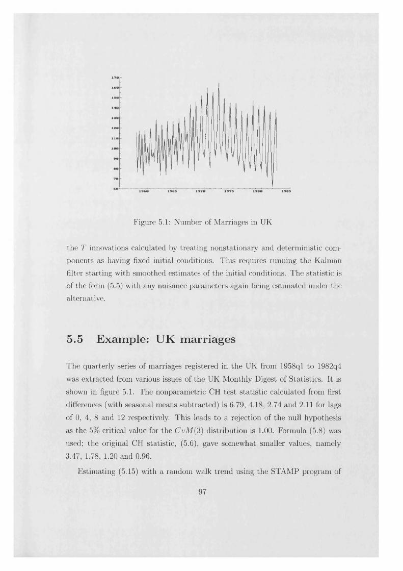
Figure 5.1: Number of Marriages in UK

the T innovations calculated by treating nonstationary and deterministic com­ponents as having fixed initial conditions. This requires running the Kalman filter starting with smoothed estimates of the initial conditions. The statistic is of the form (5.5) with any nuisance parameters again being estimated under the alternative.

5.5 Example: UK marriages

The quarterly series of marriages registered in the UK from 1958ql to 1982q4

was extracted from various issues of the UK Monthly Digest of Statistics. It is

shown in figure 5.1. The nonparametric CH test statistic calculated from first

differences (with seasonal means subtracted) is 6.79, 4.18, 2.74 and 2.11 for lags

of 0, 4, 8 and 12 respectively. This leads to a rejection of the null hypothesis

as the 5% critical value for the CvM (3) distribution is 1.00. Formula (5.8) was

used; the original CH statistic, (5.6), gave somewhat smaller values, namely

3.47, 1.78, 1.20 and 0.96.

Estimating (5.15) with a random walk trend using the STAMP program of

97

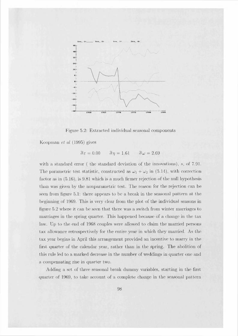
Sea_ 3=

Figure 5.2: Extracted individual seasonal components

Koopman et al (1995) gives

c t e = 0 . 0 0 (TT] = 1.61 c t u j = 2.69

with a standard error ( the standard deviation of the innovations), s, of 7.91. The parametric test statistic, constructed as lu\ -f uji in (5.14), with correction factor as in (5.16), is 9.81 which is a much firmer rejection of the null hypothesis

than was given by the nonparametric test. The reason for the rejection can be

seen from figure 5.1: there appears to be a break in the seasonal pattern at the beginning of 1969. This is very clear from the plot of the individual seasons in

figure 5.2 where it can be seen that there was a switch from winter marriages to

marriages in the spring quarter. This happened because of a change in the tax

law. Up to the end of 1968 couples were allowed to claim the married persons tax allowance retrospectively for the entire year in which they married. As the

tax year begins in April this arrangement provided an incentive to marry in the

first quarter of the calendar year, rather than in the spring. The abolition of

this rule led to a marked decrease in the number of weddings in quarter one and

a compensating rise in quarter two.

Adding a set of three seasonal break dummy variables, starting in the first

quarter of 1969, to take account of a complete change in the seasonal pattern

98

leads to the following estimates of the parameters:

a £ = 2.42 = 1.59 = 1.36

withQ( 9,7) = 12.54 H(32) = 0.77 N = 0.22 5 = 5.66

where Q(P,f) is the Box-Ljung statistic based on P residual autocorrelations but with / degrees of freedom, H is a heteroscedasticity statistic and N is the Bowman-Shenton normality test; see Koopman et al. (1995). The t —statistics for the seasonal break dummies are -8.33, 7.58 and 2.09 respectively. There is a big reduction in the estimate of the seasonal parameter, au, which no longer needs to be such as to allow the stochastic seasonal model to accommodate the change, and the equation standard error, s, has fallen considerably.

The modified nonparametric CH test statistics carried out on the residuals obtained from regressing first differences on seasonal means and the seasonal break dummies are 2.71, 2.06, 1.69 and 1.58 for m = 0,4,8 and 12 respectively for (5.8) and 2.18, 1.80, 1.57 and 1.50 for (5.6). Thus for m = 4 and 8 the null of a constant seasonal pattern is not rejected at the 5% level of significance since the critical value for CvM(§) is 1.69. The corresponding parametric test statistic, calculated from the estimated irregular component, is 9.59 indicating that there is still stochastic seasonality. This is backed up by the fact that estimating the model with a fixed seasonal gives a significant Box-Ljung statistic of Q(9,8) = 22.38 while the fourth order residual autocorrelation, r(4), is 0.33.

Although it is difficult to make firm statements about power on the basis of the above results the contrast between the parametric and nonparametric tests is striking. Furthermore, the statistic in (5.6) seems to be smaller than the one based on (5.8). Estimating the model under the null hypothesis and making the correction in formula (5.8) analytically as 7f(\j) = cr% + 2(1 — cos A)<7 gave a test statistic of 6.19 with no break and 2.26 with a break. Both figures are consistent with the nonparametric correction for moderate lag length. On the other hand if the estimated parameters under the alternative are used, the test statistic in the modelled break case is 9.39 which is not far below the figure of 9.59 reported in the previous paragraph.

99

5.6 Tests on groups of seasons

Tests to be applied to a group of seasons can be set up by constructing A' ma­trices with fewer rows and with seasons not necessarily contrasted with adjacent ones. If we are contrasting two seasons m periods apart then the A' matrix is a vector such as A '= ( 100 —10), while if the observations have been differ­enced, the corresponding vector is A' = (1 1 1 0 0). This is just a reflection of the identity Am = (1 + L + ... + Lm_1) A. The A' matrix for testing the stability of a group of si seasons has (si — 1) rows constructed in this way.

What kind of model might a test on a group of seasons imply? One possibility is a partially periodic one in which different models are assumed for two groups of seasons. Suppose there are s\ seasons in the first group and s2 in the second and + s2 = s. Then

Vt = /4*° + l t k) + 4 k\ * = 1,2, (5.17)

where the seasonal, 7^ , is modelled by a set of s*,, k = 1,2 time-varying dummies which embody the zero sum restriction over the group. If a group has only one season then the seasonal component is not needed. The trends can be assumed to have slopes for more generality so that

/4*° = /4-i + A -i + %(fc)> V a r(4 k)) = it* t , k = 1,2.

= / ? S + C f \ Var(dk)) =

More generally, the use of the state space form allows parameters and compo­nents common to both groups. For example in the present model the irregular terms can have the same variance. In any case the point is that one may wish to test the hypothesis that the seasonals in 7^ and/or 7^ are deterministic.

For tests of groups of seasons, making the correction to the smoothing error statistics is difficult and so if parametric tests are to be used the innovations tests seem like the best option.

Note that if there are as many groups as seasons, then each season has its own trend, which is independent of the others. A joint test for nonstationarity of all the series is obtained by applying the dummy variable test setting A to

100

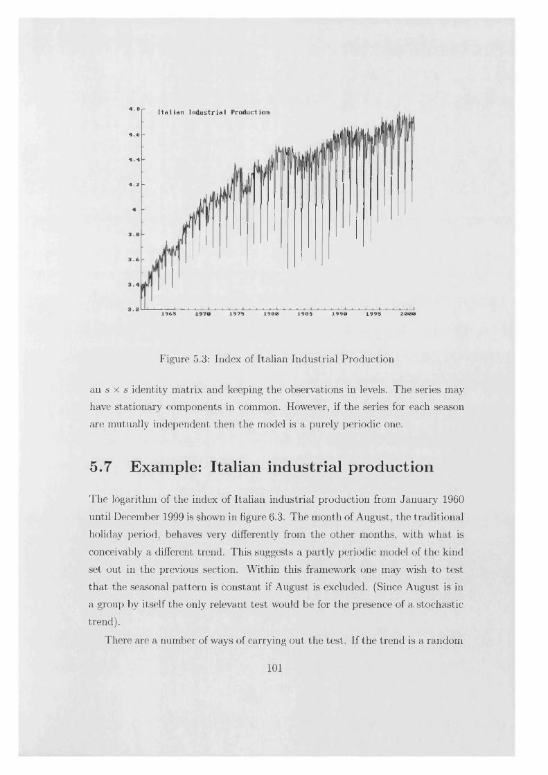
4 .8 I ta l ia n Industr ia l Production

4 .6

4 . 4

4.2

1965 1975 1980 1985 1990 20001995

Figure 5.3: Index of Italian Industrial Production

an s x s identity matrix and keeping the observations in levels. The series may have stationary components in common. However, if the series for each season

are mutually independent then the model is a purely periodic one.

5.7 Example: Italian industrial production

The logarithm of the index of Italian industrial production from January 1960

until December 1999 is shown in figure 6.3. The month of August, the traditional

holiday period, behaves very differently from the other months, with what is

conceivably a different trend. This suggests a partly periodic model of the kind

set out in the previous section. Within this framework one may wish to test

that the seasonal pattern is constant if August is excluded. (Since August is in

a group by itself the only relevant test would be for the presence of a stochastic trend).

There are a number of ways of carrying out the test. If the trend is a random

101

walk with drift, the nonparametric test can be carried out on the differenced observations with seasonal means subtracted. The A' matrix is formed by taking an 1x2 matrix and deleting the two rows which would pick up data on August ( the differenced August and September figures both depend on August).

If the trend contains a stochastic slope so that second differencing is appro­priate, the nonparametric test appears to run into problems as August affects three observations in each year.

The parametric test requires fitting a partly periodic model. If this is done, the A' matrix is a 10 x 12 matrix of the type shown in (5.4) except that there is no row corresponding to August or September.

Applying the full CH test to first differences gives ^ (1 0 ) = 4.60, which rejects the null at the 5% level, since the critical value is 2.75. If A = I 12, the test is for stochastic seasonality and a stochastic slope and the test statistic is 0^ ( 10) = 4.74. Dropping the 8th and 9th rows of the I 12 matrix, so as to exclude August, gives cja(10) = 4.32, as compared with a 5% critical value of 2.54, so the partly periodic model which excludes August still appears to display stochastic seasonality.

5.8 Seasonal unit root tests

The test of Hylleberg et al. (1990) - HEGY- is related to CH in that it is testing the null of a nonstationary seasonal against the alternative of a stationary seasonal; thus it parallels the relationship between (augmented) Dickey-Fuller test and KPSS. As with the CH test the distribution changes if seasonal trends are included in the model; see Smith and Taylor (1998).

Using arguments similar to those of Perron (1989), it can be conjectured that the performance of the HEGY test is affected by the presence of structural breaks in the seasonal pattern. Indeed, Smith and Otero (1997) have shown, via simulation experiments, that a change in the deterministic seasonal pattern results in a corresponding power loss for the seasonal unit root tests. They then tabulate new critical values for the HEGY tests which account for structural breaks. Unlike our tests of sections 3-4, their critical values depend on the

102

location of the breakpoint.

The asymptotic distributions of the HEGY statistics in the presence of ne­glected structural breaks in the seasonal pattern have been derived by Lopes and Montanes (1998) as functions of the break magnitude, the breakpoint loca­tion and the variance of the innovation. They show that all the relevant HEGY statistics asymptotically diverge, although in finite samples the probability of rejecting the unit root null hypothesis may become very low. Most of the simu­lation results of Smith and Otero (1997) are justified analytically, and the role of the break magnitude in obtaining those results is clarified

The papers by Franses and Vogelsang (1998) and Balcombe (1999) consider a single breakpoint at an unknown position and propose inf-type tests for seasonal unit roots that extend the framework of Perron and Vogelsang (1992) and Zivot and Andrews (1992) respectively. The advantage of these unconditional tests is that they cover the case of endogenous breakpoints. However, when a change in the seasonal pattern is caused by some exogenous event (as with the policy change affecting UK marriages) the unconditional testing approach is likely to favour the null hypothesis of unit roots.

If the unobserved components model is a good approximation for a time se­ries, then the alternative hypothesis in the HEGY test corresponds to seasonality being deterministic. There is then a paradox in that there are more parameters under the null. Further, the autoregressive approximation may be very poor. Suppose, for simplicity, that the model is a random walk plus seasonal plus irregular with just two seasons. Then

^ 2 Vt — (1 — L 2 )yt = (1 + L)rjt + (1 — L)ut + (1 — L 2 )et (5.18)

If either the level or seasonal variance is small relative to the irregular variance, the right hand side of the above expression is close to the invertibility boundary. When there are more than two seasons there axe more potentially deterministic terms to worry about.

103

5.9 Test of Seasonality

The CH test takes the null to be deterministic seasonality. Sometimes we may wish to test whether there is any seasonality at all. One strategy is to carry out the CH test and if this does not reject, a test of significance of the seasonal coefficients is carried out. Such a test, based on a fitted structural time series model is implemented in the STAMP package. However, it has the disadvantage that it will indicate no seasonal effects in a situation where seasonality has become less pronounced over time. This is precisely the kind of behaviour noted by Canova and Hansen (1995, p 24-50) in their analysis of US macroeconomic series. Another strategy would be to test for nonstationary seasonality using partial sums computed without fitting seasonal dummies. Such a test will have power against deterministic seasonality2 and it has the advantage that two tests are replaced by one. A modification of the nonparametric test would be to fit seasonal dummies when calculating the denominator of the test statistic. This makes no difference to the asymptotic distribution under the null hypothesis and it could increase power. The parametric test is best carried out by estimating the nuisance parameters from the general model with a stochastic seasonal fitted. However, using estimates from a model with deterministic seasonal, or indeed no seasonal at all, would still be valid. Proceeding in this way may be attractive with, say, weekly data where fitting a stochastic seasonal can be somewhat complex and time consuming.

If the CH test statistic is formed without fitting seasonal dummies, its asymp­totic distribution under the null will be a function of Brownian motion rather than of a Brownian bridge. It is still of the Cramer-von Mises family. The 5% critical values for one, two and three degrees of freedom - the last appropriate for a full test on quarterly data - are 1.65, 2.63 and 3.46 respectively; see the tables in Nyblom (1989) and Hobijn and Franses (2000). The 5% critical value for eleven degrees of freedom is 9.03. For the reasons given in section 4, the as­ymptotic distribution is unaffected by the inclusion of a constant or a constant

2 Following a similar line of argument to the one used by Hobijn and Franses (2000, appendix) in a somewhat different context, it can be shown that the test will be consistent against deterministic seasonality.

104

and a time trend.As an example we consider the logarithm of the ratio of the first decile to

the median for quarterly wages of US males from 1979ql to 1999q3; see Harvey and Bernstein (2000) for further details. While there are clear deterministic sea­sonal patterns in the deciles, these almost cancel in the log ratio leaving a weak seasonal which changes over time. The question is whether this seasonal is any sense significant. Fitting a random walk plus seasonal plus noise model gives a chi square statistic for the seasonals at the end of the series, 1.83, which is not significant, but this may be unreliable if seasonality becomes less pronounced over time. If the seasonal component is omitted, the fourth order residual auto­correlation, r(4), takes a value of 0.24 which is rather high. Unfortunately the distribution of this statistic is not known. However, the Q(8 ,7) statistic is 10.70 which is not significant. Our parametric seasonal test is 2.60 so it doesn’t quite reject at the 10% significance level for which the critical value is 2.83. This backs up the evidence from the other statistics which is that there is some indication of a weak seasonal pattern.

The nonparametric statistics 0.42, 0.48 and 0.49 for m — 4,8 and 12 so again it appears to have very low power.

As a final point, note that the test can be applied to a seasonally adjusted series to see if the adjustment has been effective. This assumes that the adjust­ment has been done by means of moving averages, rather than by regressing on seasonal dummies. If dummies have been used, then the test statistics have the usual CH distribution.

5.10 Testing for the presence o f trading day ef­fects

Cleveland and Devlin (1980) showed that peaks at certain frequencies in the esti­mated spectra of monthly time series indicate the presence of trading day effects. Specifically there is a peak at a frequency of 0.348 x27r radians, with the possi­bility of subsidiary peaks at 0.432 x27r and 0.304x27t radians. An option in the output of the X-12-ARIMA program provides a comparison of the estimates of

105

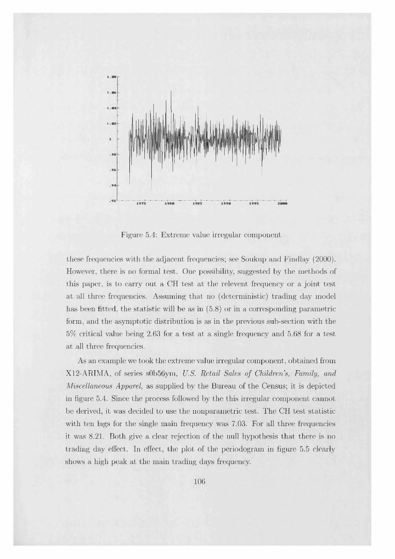
1

1

1

1

Figure 5.4: Extreme value irregular component

these frequencies with the adjacent frequencies; see Soukup and Findlay (2000). However, there is no formal test. One possibility, suggested by the methods of this paper, is to carry out a CH test at the relevent frequency or a joint test at all three frequencies. Assuming that no (deterministic) trading day model

has been fitted, the statistic will be as in (5.8) or in a corresponding parametric form, and the asymptotic distribution is as in the previous sub-section with the 5% critical value being 2.63 for a test at a single frequency and 5.68 for a test

at all three frequencies.

As an example we took the extreme value irregular component, obtained from

X12-ARIMA, of series s0b56ym, U.S. Retail Sales of Children’s, Family, and Miscellaneous Apparel, as supplied by the Bureau of the Census; it is depicted

in figure 5.4. Since the process followed by the this irregular component cannot

be derived, it was decided to use the nonparametric test. The CH test statistic

with ten lags for the single main frequency was 7.03. For all three frequencies

it was 8.21. Both give a clear rejection of the null hypothesis that there is no

trading day effect. In effect, the plot of the periodogram in figure 5.5 clearly

shows a high peak at the main trading days frequency.

106

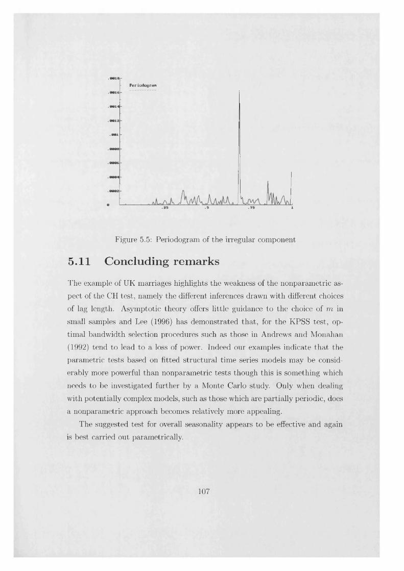
P e r io d o g r a n

Figure 5.5: Periodogram of the irregular component

5.11 Concluding remarks

The example of UK marriages highlights the weakness of the nonparametric as­

pect of the CH test, namely the different inferences drawn with different choices

of lag length. Asymptotic theory offers little guidance to the choice of m in

small samples and Lee (1996) has demonstrated that, for the KPSS test, op­timal bandwidth selection procedures such as those in Andrews and Monahan

(1992) tend to lead to a loss of power. Indeed our examples indicate that the

parametric tests based on fitted structural time series models may be consid­erably more powerful than nonparametric tests though this is something which

needs to be investigated further by a Monte Carlo study. Only when dealing

with potentially complex models, such as those which are partially periodic, does

a nonparametric approach becomes relatively more appealing.

The suggested test for overall seasonality appears to be effective and again

is best carried out parametrically.

107

Chapter 6

C ointegration in structural tim e series m odels

A structural time series model is set up in terms of unobserved components, such as trends, and cycles, which have a direct interpretation; see Harvey (1989), Kitagawa and Gersch (1996) and Young (1984). In a multivariate structural model we have cointegration when the number of stochastic trends is less than the number of the series (common trends).

This chapter deals with representation, estimation and test of cointegrated structural time series models. Identification of the cointegrating vectors is dis­cussed and order and rank conditions for identification are given. A number of links with the literature on vector autoregressions are established. In particular, it is showed that a cointegrated structural time series model can be represented as a vector autoregression, and it is also explained how to compute the VAR coefficients using the filtering algorithm given in Koopman and Harvey (1999).

The tests developed in chapters 3 and 4 can be naturally applied to make inference on the dimension of the cointegration space and to test for prespecified cointegration vectors. Maximum likelihood estimation of cointegrated structural time series models is done by putting the models in state space form and com­puting the prediction error decomposition form of the likelihood function, using the Kalman filter to obtain the innovations. Efficient estimation requires incor­porating the common trend restrictions. An empirical example is provided with the series of US GNP and Investment.

In summary the chapter proceeds as follows. Section 6.1 reviews the concept

108

of cointegration, the VAR/MA/ECM representations of cointegrated systems and the Granger Representation Theorem. In section 6.2 representation and identification of cointegrated system in the structural time series framework are considered and links with the VAR representation are established. Estimation and test of cointegrated structural time series are discussed in section 6.3 and an empirical example is provided in section 6.4.

6.1 Cointegration and the Granger representa­tion theorem

We say that a vector process x* is integrated of order d, denoted I(d), if A dx t is a covariance stationary process with positive definite spectrum at frequency zero; slightly different definitions of integrated processes are possible, see Davidson (1999). The vector process xf is said to be cointegrated of order d ,g , denoted C I(d ,g ), if (i) each component of x* is 1(d) and (ii) there exists a nonzero vector b such that b'x* is I(d —g), where d > g > 0. The vector b is called cointegrating vector. In the following we will restrict attention to C7(l, 1) processes.

Consider an TV-dimensional process x* that in first differences has the moving average representation

Ax* = S + C(L)et, (6 .1)

where et is a TV-dimensional i.i.d. process with zero mean and positive definite variance, 6 is a drift and the matrix polynomial in the lag operator C(L) =

C jlJ satisfies Y°jLo IIQII < 00• From (6.1) it follows that x* is cointe­grated of order 1,1 if C(l) is not of full rank. Further, the number of linearly independent cointegrating vectors is given by R = TV — rank(C( 1)).

In fact, first note the identity

C(L) = C( 1) + (1 - L)C*(L), (6.2)

where C*(L) is defined by C* = Cj, i = 0,1,... Then integrate (6.1) toget

tx* = Xq + St + C(l) ^ 2 £s + C*(L)et, (6.3)

S=1

109

with x j = x0 — C*(L)eq. Clearly, the nonstationary part C (l) £s is anni­hilated only if there exist nonzero vectors b such that b 'C (l) = 0. This, in turn, is true if and only if (7(1) is not of full rank. In particular, call S the left null space of (7(1), i.e.

S = {b: b 'C (l) = 0} .

Then S is the cointegration space, i.e. all the elements b in this space make the linear combination b'x* stationary. By a well known result of linear algebra the dimension of S is R = N — rank(C(l)), and thus R is the maximum number of linearly independent cointegrating relations. Usually we want to collect R of these linearly independent vectors into a (N xR ) matrix B=[bi b 2 ... b #].

For any b we have the following cointegrating relation

b'x* = b 'x j + b 'St + b'<7*(L)e*, (6.4)

i.e. b'x* is stationary around the linear trend b 'St. If S G S 1-, where S 1- is the space orthogonal to S , the equilibrium relation (6.4) does not contain a time trend.

If there were not cointegration, the MA representation (6.1) could be inverted to yield the autoregressive representation of the process in first differences. With cointegration this is no longer possible for the presence of unit roots in the matrix polynomial C(L).1 However it is possible to construct the autoregressive representation in the levels of the process, inverting (1) as showed in Engle and Yoo (1991) by factorizing C(L) appropriately. This inversion is the essence of the Granger representation theorem, which establishes an isomorphism between the MA and AR representations of a cointegrated system. Further, by a simple reparametrization, the system can be put in error correction form. The theorem is stated below for the case of a driftless process.

T heorem 18 (Granger Representation Theorem). Let et be a N-dimensional i.i.d. process with zero mean and positive definite variance. Let C{z) be a N x N matrix polynomial such that

(a) |(7(z)| = 0 has no roots \z\ < 1,(b) \C(z)\ = 0 has N — R roots z = 1 or equivalently rank(C(l))— N — R,

1 The characteristic equation |C(z)| = 0 has the solution z = 1 if C{ 1) is not of full rank.

110

(c) C (l)A = 0, B 'C (l) = 0 for two N x R matrices A, B with rank R.Then a process cc, has the MA representation

Ax, = C(L)et, (MA)

if and only if it has the AR representation

IT(L)x, = et, (AR)

where the matrix polynomial II (z) satisfies(a)’ |II(z)| = 0 has no roots \z\ < 1,(b)’ |II(z)| = 0 has R roots z = 1 or equivalently rank(II(1)J= R,(c)’ 11(1) = AB'.

The theorem is proved in Engle and Granger (1987), Engle and Yoo (1991) and Johansen (1991). Now define the polynomial matrix T(L) by

n(L) = n (i)L + ( i - L ) r ( L ) ,oo

i.e. r 0 = n 0, I \ = — ^2 Ilj, i = 1,2,... Then the process x, of the theoremj=i+1

has the further representation

T(L)Ax, = AB'x,_i + £t, (-^0

called error correction form.The matrix B contains R linearly independent cointegrating vectors, i.e.

B'x, is 7(0) and represents the equilibrium relationships between the variables. The error correction representation (EC) allows the modeling of the process as deviation from that equilibrium, incorporating both the short run and the long run in the system. The matrix A contains the adjustment coefficients and, together with the autoregressive parameters IYs, represents the short run dynamics.

The importance of the theorem is that the representations (AR) and (EC) are easy to handle and estimate, e.g. if we assume Gaussianity for the innovations. Then it is possible to construct tests for cointegration by looking at (the rank of) the long run matrix 11(1), and in case of positive answer incorporate this restriction into the error correction form obtaining a fully efficient maximum likelihood estimator (Johansen 1988, 1991 and 1992).

I l l

In the case of a drift, a linear trend of the form do + d it must be added in the right hand side of (EC). The restriction C (l)d i = 0 excludes a quadratic trend in the levels of the process while the restriction di = 0 excludes a linear trend in the cointegration relation; see also Pesaran and Shin (1994).

Consider now the problem of identification. Any basis for the dimensional space S can be taken as a valid set of cointegrating vectors, i.e. it can describe the equilibrium relationships of the system. The non uniqueness of the coin­tegrating vectors is evident in that, for every R x R non singular matrix Q, if B'x* is stationary so is QB'x*. In other words, when we estimate the (EC) representation of the system, the set of cointegrating vectors B and the adjust­ment coefficients A are not identified, since they are observationally equivalent to A = AQ -1 and B = BQ' for every non singular Q .2

Identification thus requires placing constraints on B, in order to work out the R 2 elements of the matrix Q. At a first stage, these constraints can simply be restrictions implied by some normalization rule, as in the case of Johansen’s maximum estimate of B obtained via reduced rank regression (see Johansen, 1988). However, in general these will not produce interpretable or economically meaningful equilibrium relationships. Thus, in a second stage economic theory should supply help, providing the necessary overidentifying restrictions on the cointegration space to work out a unique set of cointegrating vectors. This identification problem, which is relevant for empirical studies, is thoroughly analyzed by Pesaran and Shin (1995).

6.2 Representation of cointegrated structural tim e series

A structural time series model is set up in terms of orthogonal components which have a direct interpretation, e.g. trend, cycle, seasonal, etc. Harvey (1989) gives a full account of this modelling strategy. Here we assume for simplicity that the A-dimensional process x t is made up of only two components,

x t = /i* + ut , (6.5)2 Only the long run matrix 11(1) is identified, as 11(1) = AB' = AB'.

112

where n t is a ’’trend” (long run component), and ut is a ’’cycle” (short run component).

We assume that the cycle ut is a 7(0) process as defined in the previous section, i.e. it is a covariance stationary process with positive definite spectrum at frequency zero.

In the structural time series framework, the trend fit is often modeled as a local linear trend (see Harvey, 1989)

= Mt-i + <*t-i + T7t, (6.6)

f i t = f i t - i + C t j ( 6 . 7 )

where is i.i.d. with zero mean and variance diag (E77, E ^ ). In this case,if E^ is of full rank, y tt is an 7(2) process.

Since in this chapter we axe mainly interested in C7(l, 1) processes, it will be assumed below that E^ = 0 , i.e. that the slope 8t is fixed and equal to S. Then the trend is a random walk with drift and the structural time series model(6.5) can be compared to the models considered in the previous section.

6.2.1 Common trends and cointegration

Cointegration is directly connected with the existence of common trends. Let K be the rank of E77, 0 < K < N. Since there exists a (N x K) matrix © such thatE^ = © 0 ', we can reformulate the model in terms of only K orthogon,al trends.In particular we can write rjt = ©r/+, with r j f ^ i.i.d. (0,7^), and the model becomes

xf = Q fif + /x* + St + ut (6 .8)

* 4 = l 4 - i + V t (6.9)

where yC = ( o' Ji ) with the N — K dimensional vector Jt obtained from

the initial conditions on the trend.© is called the matrix of factor loadings. Note that © is not unique, since

for any (K x K ) orthogonal matrix H, © = ©H is another square root of E^.Therefore identification of the loadings requires placing K (K — l) /2 constraints

113

on ©. The simplest way to enforce identification is to assign a lower triangular structure to ©, that is assuming [0]i . = 0 for j > i. Of course, this identification scheme of the loadings, which implies a causal chain in the trends, is arbitrary. However, after estimating a model set up in that way, it is possible to look for an appropriate rotation H of the loadings that has an economic interpretation (as done in Harvey et al. 1995).

From the formulation (6 .8)-(6.9), it is easy to see that the process x* is (7/(1,1), with the cointegration space being the left null space of 0 ,

S = {b : b'© = 0}.

This space has dimension R= N — K , i.e. there exist R linearly indepen­dent cointegrating vectors bi, b 2, •••, b# that we can collect into a matrix B = (bi b2 ...b /j) . Note that S is independent of the rotation of the trends, since 0 = b '0 = b ' (0H ) for every rotation H.

As in the previous section, if 5 e S 1- a linear trend is excluded from the cointegrating relations. But since S 1- is also the range of 0 , when S E<5r L there exists a A-dimensional vector 6+ such that S = QS+. Then the slope can be incorporated into the common trend n f , adding <5+ in the right hand side of equation (6.9) and removing 6 t from (6 .8).

6.2.2 Identification o f the cointegrating vectors

Let the dimension of the cointegration space be R and let B be an N x R matrix that contains R linearly independent cointegrating vectors. Then, as we have seen before, B satisfies

B '0 = 0 , (6.10)

where © is a N x K matrix of factor loadings, with K = N — R, which can be efficiently estimated in the structural time series framework; see section 6.3.

As in section 6.1, identification of B (i.e. identification of a unique set of cointegrating vectors) requires placing additional restrictions on the elements of B other than (6.10). As for a simultaneous equations model, we can obtain an order condition and a rank condition for identification of B.

114

Since (6.10) defines a system of K R equations in N R unknowns, the order condition for identification requires imposing p > R2 extra restrictions. Let these be linear and denoted as

a 'W = u/, (6.11)

where a =vec( B), W is a known N R x p matrix and a; is a known p x l vector. Note that (6.11) has to include R inhomogeneous restrictions, e.g. obtained by normalizing one element in each cointegrating vector.

Then, by the usual argument on the existence of a unique solution in systems of linear equations, we have that the rank condition for identification is

rank{* ) = N R , (6.12)

where ^ = (I r ® 0 , W ).The identifying restrictions (6.11) should have economic interpretation as

opposed to being arbitrary. However, arbitrary identification schemes axe often employed in the literature. For example, we could think of partitioning our cointegrated vector process xt into K trending variables and R variables X21 cointegrated with the previous ones. If we correspondingly partition © into (©5,02)': where ©i is K x K and ©2 is R x K, we have that the matrix B of cointegrating vectors becomes

B = C<3',Ir )’ ,

with f3 = — ©2©]-1. The resulting system is sometimes called Phillips triangular system, as it corresponds to the model analyzed by Phillips (1991, 1994); seealso Harvey and Koopman (1997). In this case, the R 2 restrictions (6.11) areobtained by setting the R x R lower submatrix of B equal to the I r .

6.2.3 VAR representation

The following proposition extends theorem 18, the Granger Representation The­orem, by showing that a structural time series model with common trends can be represented as cointegrated VAR (and as error correction model).

115

Proposition 19 Let x* be generated by the model (6.5)-(6.7) with ££ = 0 and ra n k e r /) = K, 0 < K < JV, where the short run component Ut is a 1(0) process with positive definite spectrum everywhere. Then cc* can be represented as a cointegrated VAR.

The proof amounts to showing that Ax* has a MA representation that satisfy conditions (a) and (b) of theorem 183 . This is most easily done by considering the spectrum of Ax*, which is given by

FaxW = (27r)_1Er? + 2(1 - cos X)FU(\), - ir < X < 7r,

where Fu(A) is the spectrum of u*.

Clearly, rank(Fax(0)) = K , thus condition (b) is satisfied. Then, since we have assumed Fu(A) positive definite everywhere, we have that Fax(A) is positive definite for A ^ 0. This is equivalent to saying that, except for the K unit roots of condition (b) above, all the other roots of the matrix polynomial in the MA representation of Ax* are outside the unit circle, and so condition (a) is satisfied too.

Thus we have established that a cointegrated structural time series can be represented as a vector autoregression with reduced rank long run multiplier (and with in principles an infinite number of lags). However, note that estimating a finite order VAR can be a bad approximation if the true model is of the type(6.5)-(6.7), as the reduced form of these models is often close to the region of noninvertibility; see Harvey (1989). This could happen, for example, if the ’’size” of £77 is small or if there are comovements also at business cycle frequencies.

After having established that, under mild assumptions, a cointegrated struc­tural time series model admits a VAR representation, the next step is to derive the VAR coefficients from the parameters of the structural model. Koopman and Harvey (1999) have proposed a numerical algorithm that can be adopted, as it is valid for any state space model. Their result is outlined in the following section.

3 To check condition (c) is not necessary as it is implied by (b).

116

6.2.4 Com puting the VAR coefficients

Koopman and Harvey (1999) have obtained algorithms to compute the obser­vation weights for signal extraction and filtering in a state space model like

x* = ZtOt-t + dt + Et, (6.13)

cx-t = Gt&t-i + Ct + RtTju (6* 14)

see section 2.2 for the details on the state space representation of time series.The filtered estimator of the state vector in the next time period, that is the

estimator of at based on information available at time t — 1, can be written as

t - iat\t—i = ^ ■>

j =i

where the W j Js are appropriated weights, that can be computed using the algo­rithm in Koopman and Harvey (1999). Then the one-step ahead predictor of xt becomes t - i

x,|(-l =j = 1

where w* = ZtWj.Since xt = 5it\t-i + vf, with v t being the one-step ahead prediction error, the

weights w* are the coefficients of the autoregressive representation for a time invariant model when the filter is in steady state. Using the notation of section 6.1 we have t - i

* = £ n fcxt_fc + v*, Var(vt) = F,k=1

where n*; = w*_k. Clearly, for the multivariate model with common trends of section 6.2.1 it will hold that |I — n^l = 0; see Koopman and Harvey (1999) for a numerical example.

6.3 Estim ation and test

The common trends test of chapter 4, section 4.4, can be naturally applied to a structural time series model of the type (6.5)-(6.7) to make inference on the

117

number of cointegrating relations. In a model with fixed slope, the statistic € k , n (4.18), constructed using z t = (1, t)' as regressors, tests the null hypothesis that the cointegration space has dimension R = N — K against the alternative hypothesis that the dimension is lower; note the direction of the alternative hy­pothesis, opposite with respect to Johansen’s tests. In practice, one can compute fo,jv, £i,jv, ••• sequentially, stopping at the first non-rejection (although, strictly speaking, this sequential procedure would be affected by pretesting bias).

A structural time series model which incorporates common trends restrictions can then be estimated. Under Gaussianity, maximum likelihood estimation of a model like (6.5)-(6.7) can be carried out by putting it in state space form and using the (multivariate) Kalman filter to evaluate the Gaussian likelihood function in the time domain; see section 2.2 4.

In particular, the state space form for the common trend model (6.8)-(6.9), when u t is a white noise, can be obtained by setting

in (6 .13)-(6 .14), with the N x K matrix of factor loadings © partitioned as 0 = (©i, @2/ , where ©1 is K x K and ©2 is R x K.

Note that in this formulation 8 is treated as an unknown parameter whereas the initial condition JL is included in the state vector. An alternative approach is to treat also JL as an unknown parameter, to be estimated jointly with 8 by the GLS algorithm of section 2.3.

Given ©, an asymptotically efficient estimator for 8, alternative to the GLS, is given by

8 (0 ) = (0 '© )_10'Ax^,

where Ax* = (x^ — Xi )/{T — 1). This is obtained from concentrating 8 outof the spectral likelihood function for the observations in first differences, and4 The menu-driven program Stamp 5.0 by Koopman et al. (1995) is designed to estimate most of the standard (multivariate) structural time series models, also with common com­ponents and regression effects. Alternatively, more flexibility can be achieved by using the matrix programming language Ox 2.1 together with the set of routines for state space models implemented in Ssfpack 2.2; see Doornik (1998) and Koopman et al. (1998).

, G t — I j v , dt — 0

118

intuitively from the consideration that only the contribution at frequency zero matters for the estimation of 6 , see Harvey (1989, p.453) for the expression of the spectral likelihood and the derivation of the estimator above.

A number of diagnostic tests is available to assess the adequacy of the struc­tural time series model fitted to the data. These are constructed from the one step ahead prediction errors (or ’’residuals”) in a similar way as in the Box and Jenkins methodology; see Harvey (1989 ch. 5) and Harvey and Koopman (1992).

As discussed in section 6.2.2, an important empirical issue is to identify the cointegrating relations, or -in other words- to test for restrictions on the coin­tegration space. A simple nonparametric test for a pro-specified cointegration vector b is given by the KPSS test (3.22) applied to b'x*. Similarly, the nonsta- tionarity test of section 4.2 can be used when multiple cointegrating relations are to be tested simultaneously.

Restrictions on the factor loadings matrix © that do not change its rank (overidentifying restrictions) can be tested using a Likelihood Ratio test. If the model is correctly specified, under the null hypothesis the statistic —2 (lr — lu), where lr, lu are respectively the restricted and unrestricted log-likelihood functions, is asymptotically x 2 with degrees of freedom equal to the number of restrictions (provided they do not change the rank of 0 ).

Note that restrictions on © imply restrictions on the cointegration matrix B via the relation (6.10). Thus the LR approach can also be interpreted as a test for overidentifying restrictions on B. As an example, consider a model with three variables and one trend, thus with © = (1, 6 1 , 6 2 )' and

B ' =/ , h h1 O12 O13

1 22 &23Y 1 U22 y23 y

Here the constraint 61 = 6 2 = 6 corresponds to the cross equation restriction

&12 + &13 — ^22 + &23- (6.15)

This can then be tested using the LR test described above. Note also that adding another restriction, e.g. 612 = 0, to (6.15) is sufficient for identification.

119

Log o f US GNP

Figure 6.1: US Real GNP and estimated stochastic trend

6.4 An example of cointegrated structural tim e series model

As an illustrative example, we consider a bivariate model for (the logarithm of)

US GNP and Investment. The data are quarterly, seasonally adjusted and refer

to the period 1951-1985. They are part of a dataset which is provided with STAMP 5.0.

Figures 6.1-6.2 show the plot of the series. A cyclical component appears

quite evident, particularly in the investment series. Harvey and Jaeger (1993)

fitted a plausible univariate structural model to the data, yielding a stochastic

cycle with estimated period of about 20 quarters (5 years). This seems to be a

good characterization of US business cycle for the years covered by the sample.

Economic theory and numerous empirical studies suggest that the series of

GNP and Investment should be nonstationary and cointegrated, possibly with

a cointegration vector equal to (1 —1)'. It is also plausible that the cyclical

120

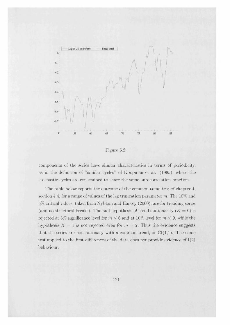
-6

-6.11

-6.2

-6.3

-6.4

5()

Figure 6.2:

components of the series have similar characteristics in terms of periodicity, as in the definition of ”similar cycles” of Koopman et al. (1995), where the

stochastic cycles are constrained to share the same autocorrelation function.

The table below reports the outcome of the common trend test of chapter 4,

section 4.4, for a range of values of the lag truncation parameter m. The 10% and

5% critical values, taken from Nyblom and Harvey (2000), are for trending series (and no structural breaks). The null hypothesis of trend stationarity (K = 0) is

rejected at 5% significance level for m < 6 and at 10% level for m < 9, while the

hypothesis K = 1 is not rejected even for m = 2. Thus the evidence suggests

that the series are nonstationary with a common trend, or CI(1,1). The same

test applied to the first differences of the data does not provide evidence of 1(2)

behaviour.

of US Investment

121

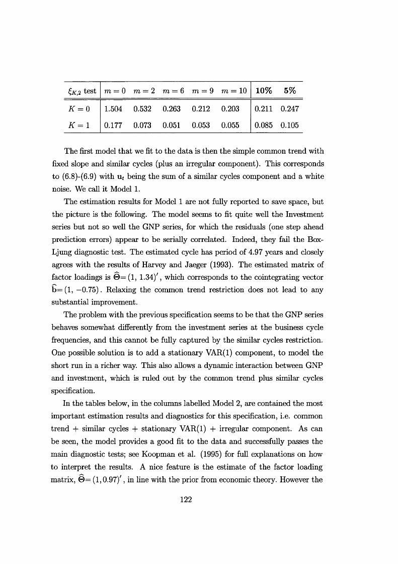
£k ,2 test m = 0 m = 2 m = 6 m = 9 m = 10 1 0 % 5%

K = 0 1.504 0.532 0.263 0.212 0.203 0.211 0.247

K = 1 0.177 0.073 0.051 0.053 0.055 0.085 0.105

The first model that we fit to the data is then the simple common trend with fixed slope and similar cycles (plus an irregular component). This corresponds to (6 .8)-(6.9) with u t being the sum of a similar cycles component and a white noise. We call it Model 1.

The estimation results for Model 1 are not fully reported to save space, but the picture is the following. The model seems to fit quite well the Investment series but not so well the GNP series, for which the residuals (one step ahead prediction errors) appear to be serially correlated. Indeed, they fail the Box- Ljung diagnostic test. The estimated cycle has period of 4.97 years and closely agrees with the results of Harvey and Jaeger (1993). The estimated matrix of factor loadings is 0 = (1, 1.34)/ , which corresponds to the cointegrating vector b = ( l , —0.75). Relaxing the common trend restriction does not lead to any substantial improvement.

The problem with the previous specification seems to be that the GNP series behaves somewhat differently from the investment series at the business cycle frequencies, and this cannot be fully captured by the similar cycles restriction. One possible solution is to add a stationary VAR(l) component, to model the short run in a richer way. This also allows a dynamic interaction between GNP and investment, which is ruled out by the common trend plus similar cycles specification.

In the tables below, in the columns labelled Model 2, are contained the most important estimation results and diagnostics for this specification, i.e. common trend + similar cycles + stationary VAR(l) + irregular component. As can be seen, the model provides a good fit to the data and successfully passes the main diagnostic tests; see Koopman et al. (1995) for full explanations on how to interpret the results. A nice feature is the estimate of the factor loading matrix, 0 = (1,0.97)/ , in line with the prior from economic theory. However the

122

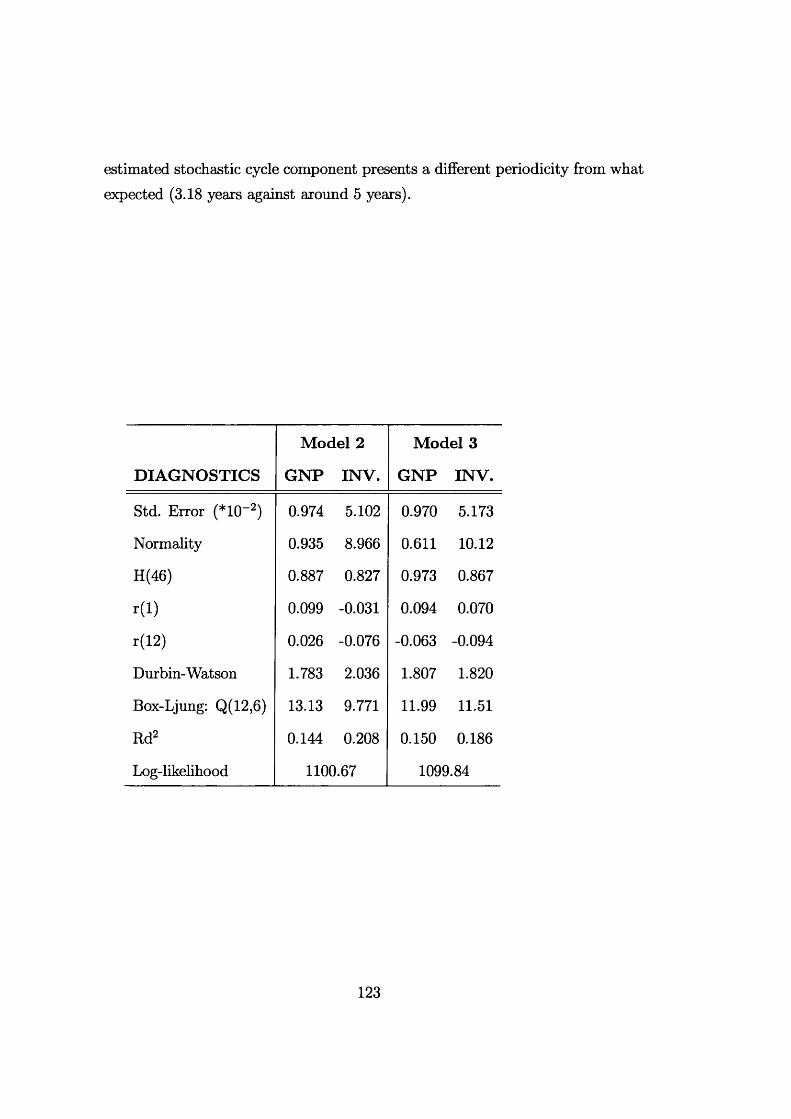
estimated stochastic cycle component presents a different periodicity from what expected (3.18 years against around 5 years).

D IA G N O STICS

M odel 2

G N P INV.

M odel 3

G N P INV.

Std. Error (*10-2) 0.974 5.102 0.970 5.173

Normality 0.935 8.966 0.611 10.12

H(46) 0.887 0.827 0.973 0.867

r(l) 0.099 -0.031 0.094 0.070

r (12) 0.026 -0.076 -0.063 -0.094

Durbin-Watson 1.783 2.036 1.807 1.820

Box-Ljung: Q(12,6) 13.13 9.771 11.99 11.51

Rd2 0.144 0.208 0.150 0.186

Log-likelihood 1100.67 1099.84

123

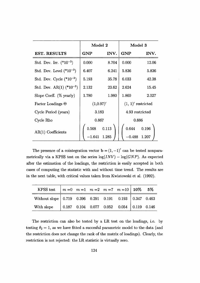
M odel 2 M odel 3

EST. RESULTS G N P IN V . G N P IN V .

Std. Dev. Irr. (*1CT3) 0.000 8.704 0.000 12.06

Std. Dev. Level (*10-3) 6.407 6.241 5.836 5.836

Std. Dev. Cycle (*10-3) 5.193 35.78 6.033 42.38

Std. Dev. AR(1) (*1(T3) 2.132 23.62 2.624 15.45

Slope Coeff. (% yearly) 1.780 1.980 1.860 2.027

Factor Loadings © (1,0.97)' (1, 1)' restricted

Cycle Period (years) 3.183 4.93 restricted

Cycle Rho 0.867 0.886

I 0.568 0.113 \ ( 0.644 0.196 |AR(1) Coefficients

\ -1.641 1.285 I I -0.488 1.207

The presence of a cointegration vector b = (1, —1); can be tested nonpara- metrically via a KPSS test on the series log(INV) — log(GNP). As expected after the estimation of the loadings, the restriction is easily accepted in both cases of computing the statistic with and without time trend. The results are in the next table, with critical values taken from Kwiatowski et al. (1992).

KPSS test m = 0 m =1 m = 2 m =7 m =10 1 0 % 5%

Without slope 0.719 0.396 0.291 0.191 0.193 0.347 0.463

With slope 0.187 0.104 0.077 0.052 0.054 0.119 0.146

The restriction can also be tested by a LR test on the loadings, i.e. by testing 02 = 1, as we have fitted a succesful parametric model to the data (and the restriction does not change the rank of the matrix of loadings). Clearly, the restriction is not rejected: the LR statistic is virtually zero.

124

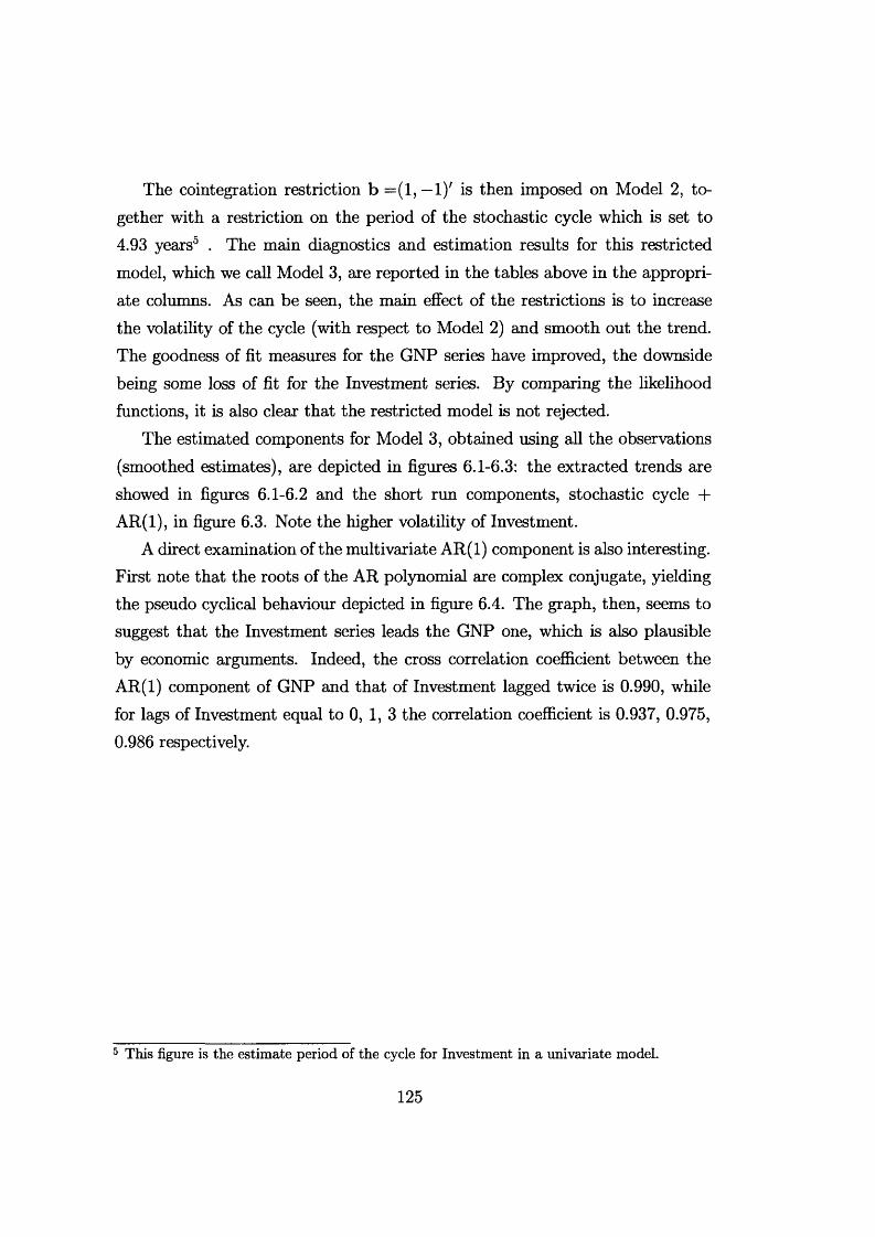
The cointegration restriction b = (1 ,—1)' is then imposed on Model 2, to­gether with a restriction on the period of the stochastic cycle which is set to 4.93 years5 . The main diagnostics and estimation results for this restricted model, which we call Model 3, are reported in the tables above in the appropri­ate columns. As can be seen, the main effect of the restrictions is to increase the volatility of the cycle (with respect to Model 2) and smooth out the trend. The goodness of fit measures for the GNP series have improved, the downside being some loss of fit for the Investment series. By comparing the likelihood functions, it is also clear that the restricted model is not rejected.

The estimated components for Model 3, obtained using all the observations (smoothed estimates), are depicted in figures 6 .1-6.3: the extracted trends are showed in figures 6 .1-6.2 and the short run components, stochastic cycle + AR(1), in figure 6.3. Note the higher volatility of Investment.

A direct examination of the multivariate AR(1) component is also interesting. First note that the roots of the AR polynomial are complex conjugate, yielding the pseudo cyclical behaviour depicted in figure 6.4. The graph, then, seems to suggest that the Investment series leads the GNP one, which is also plausible by economic arguments. Indeed, the cross correlation coefficient between the AR(1) component of GNP and that of Investment lagged twice is 0.990, while for lags of Investment equal to 0, 1, 3 the correlation coefficient is 0.937, 0.975, 0.986 respectively.

5 This figure is the estimate period of the cycle for Investment in a univariate model.

125

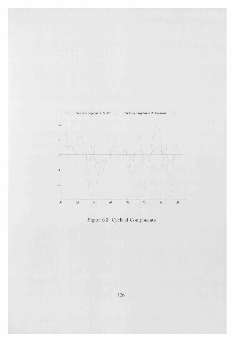
Short run component of US InvestmentShort run component of US GNP

50 55 60 65 70 75 80 85

Figure 6.3: Cyclical Components

126

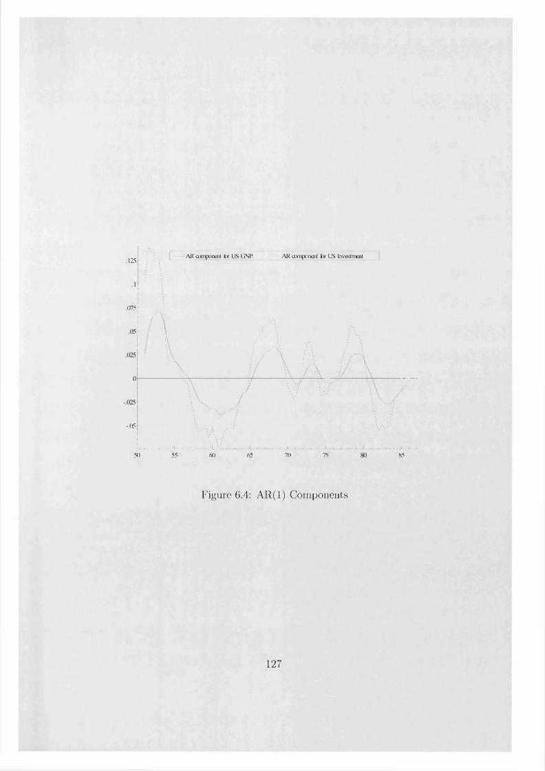
AR component for US GNP AR component for US Investment.125

.075

-.05

7550 55 60 65 70 85

Figure 6.4: AR(1) Components

127

Chapter 7

E stim ation and tests o f certain dynam ic panel data m odels

In this chapter we consider panel data models where the individual effects are modeled as individual specific random walks. The likelihood function of the models is written in the prediction error decomposition form as explained in chapter 2. Imposing the constraint of a common signal-to-noise ratio across individuals makes the maximum likelihood estimator computationally feasible also when the number of units in the cross section is large. The reason is that the same univariate Kalman filter applies to each equation in turn and numerical optimization is with respect to a single parameter only. Testing for exogeneity of the regressors and estimation with few time observations are discussed. An average LBI test for fixed effects is proposed, closely related to the cointegration test of Mc-Coskey and Kao (1998). Finally, as an example, we estimate and test a Cobb-Douglas production function from a panel of US manifacturing firms.

7.1 Introduction

Most of the literature on dynamic panel data models is centered on autoregres­sive models with time invariant individual effects. An important issue in that framework is that most of the commonly used estimators (OLS, GLS, LSDV) are not consistent when the time dimension of the panel is small; see e.g. Nickell (1981), Hsiao (1986). Proposed solutions include writing the model in first dif­ferences and estimating it by the Generalized Methods of Moments, using past

128

values of the series to instrument the lagged endogenous variable. However, if -as often is the case- the series are very persistent the instruments are only weakly correlated, and thus the properties of the GMM estimator are generally poor; see -inter alia- Arellano and Bond (1991), Ahn and Schmidt (1995, 1997), Blundell and Bond (1998, 1999) for the application of the GMM technique to panel data and Blundell et al. (2000) for a discussion of the issue of weak instruments in this context.

The panel data models considered in this chapter assume, on the other hand, a specific time varying structure for the individual effect, namely that of a ran­dom walk, but other processes could be considered with minor modifications of the arguments. Giving this structure to the individual effect can be sensible in many instances, for example in the case of a production function where it can be identified with the firm’s (unobserved) technical progress or the Solow residual.

The random walks representing the individual effects are constrained to share the same signal-to-noise ratio across individuals, similarly to the autoregressive case where the same coefficient applies for the lagged endogenous variables. Further heterogeneity is permitted by leaving unrestricted the variances of the noise.

This chapter has then some points in common with some recent literature that extends well known time series results, especially on unit roots and cointe­gration, to the case of panel data, see e.g. Im et al. (1997), Kao (1999), Phillips and Moon (2000). As in that literature, we tipically assume a large time di­mension of the panel, although we also discuss the case of few time periods. Indeed, testing for fixed effects in our framework is closely related to testing for cointegration, as done in McCoskey and Kao (1998).

The models we consider can be estimated using st at e-space techniques to obtain a consistent and fully efficient estimator under the assumption of strict exogeneity of the regressors. The likelihood function of the model is written in the prediction error decomposition form using the Kalman filter algorithm to obtain the innovations, as explained in chapter 2 . Since the same univariate Kalman filter is applied to each equation in turn and the Kalman filter recur­sions depend on a single parameter, evaluating and maximizing this likelihood

129

function is computationally feasible even when the number of individuals in the panel is large. Indeed, numerical optimization is required only for one scalar parameter, the common signal-to-noise ratio. This is the subject of sections 7.2-7.3.

In section 7.4 we propose an Hausman-type statistic for testing exogeneity of the regressors, whereas section 7.5 discusses estimation with few observations along the time dimension of the panel. The baseline model is then extended in section 7.6 by including an unobserved component common to all individuals, or common trend.

Section 7.7 considers testing for stationarity and for the presence of fixed effects. We propose an Average LBI test, constructed by taking the average of the univariate LBI statistics across individuals. The test is closely related to the panel unit root test of Hadri (1998) and the panel cointegration test of McCoskey and Kao (1998). Here we prove consistency of the test when only a fraction of the individuals have an unobserved random walk component. Finally, as an illustration, in section 7.8 we estimate a Cobb-Douglas production function for a panel of US manufacturing firms and we apply the tests described.

7.2 The baseline model

Let (Hu, x 'J , z = 1,..., N, t = 1,..., T, be a set of observations across N individu­als and for T time periods, with yit scalar and a (p x 1) vector. We consider the linear panel data regression model

Vit = x'itP+uit, (7.1)

where the regressors are strictly exogenous, (3 is a (p x 1) vector of regres­sion coefficients and uit is an error term having the following two components structure

Hit — Vit "b £iti

Vit = V i , t - 1 + V i t ,

130

(7.2)

(7.3)

fl io ~ N (0,k), K.-+00, (7.4)

(eiur}it)'\X ~ N I D (O,diag(of, gof)) , q > 0. (7.5)

The two components in the error term are an individual specific stochastic trend and an irregular disturbance respectively. The disturbances (eu^rjit) are assumed orthogonal across both time and individuals.

The individual effect is [in. It is time varying and takes the form of a random walk (stochastic trend). We impose the restriction that the signal-to-noise ratio q is the same across individuals1 . The variances of the irregular components are, in general, left unrestricted, thus allowing for further heterogeneity in the panel.

The random walk is initialized with a diffuse prior (7.4). Alternatively we could treat fao as a parameter to estimate; however, Shephard and Harvey (1990) and Shephard (1993) have shown that the diffuse prior assumption leads to better properties of the maximum likelihood estimator of q when the true value is zero. Note that if q = 0 and fao is fixed we have the standard fixed effect model, whereas if q = 0 and k is finite we have the standard random effect model, see e.g. Hsiao (1986).

Apart from including lagged values for the regressors, the dynamics of the model are the individual specific dynamics fin only; also no correlation is al­lowed across individuals. In section 7.4 the model will be extended by adding a time varying component common to all individuals (’’common trend”), by which richer dynamics and cross section correlation are obtained.

A model similar to (7.1)-(7.5), but without regressors, was proposed by Mar­shall (1992) in the context of modelling cross sections of time series, and its extension to panel data was advocated by Harvey and Koopman (1996).

The interest lies in making inference on the vector of coefficients /3 and the signal-to-noise ratio q.

Model (7.1)-(7.5) can be written in matrix notation as

Yi = X i0 + Ui, i = 1,..., iV, (7.6)

1 Other processes for the individual effects could be considered (as long as constrained to share the same autocorrelation function) with minor modifications of the arguments below.

131

where l i = (yiU ..., yiT) ' , X { = (xa , ...,x iT) ' , Ui = (u ^ ,..., uiT)f .Let =E(UiU-\Xi), i = 1, ...,7V. In our model (T.l)-(7.5) = of (It +

where H is the random walk generating matrix, i.e. a T xT matrix whose element of position (t, s) is min(i, s), and I t is a T x 1 vector of ones. The (unfeasible) Generalized Least Squares estimator of /3 is known to be

/ N \ -1 N

0gls = E xinr'Xi E (7.7)\ i=l / i=l

This is also the formula of the Maximum Likelihood Estimator of (3 when the SVs are known. When the s are not known it is possible to compute the joint likelihood of (/3, f i i , ..., Qiv) via the prediction error decomposition and maximize it numerically, as explained in section 2.3 for the case of a univariate model (AT = 1). Although not generally true, for model (7.1)-(7.5) this approach is computationally feasible even for a large number of cross section units N, since the same Kalman filter can be applied to each equation in turn. This is explained in the next section. The resulting estimator is asymptotically equivalent (as T —> 00) to the unfeasible GLS (7.7).

The model is extended in section 7.4 by including a trend component common to all individuals, showing that only few complications arise. In particular the common trend can be washed out by means of a ’’Within transformation” giving rise to a transformed model formally identical to (7.1)-(7.5). Alternatively, the common trend can be modelled explicitly and included in the likelihood function.

7.3 Estim ation o f the model

Consider Ui = Yi — Xi/3 from (7.6) with E (UJ7l\ Xi) = It is known that there exists a lower diagonal matrix L with ones on the main diagonal and a diagonal matrix F such that

n - ' = a ^ L 'F - 'L , i = l,...,N .

As explained in section 2.3, the above decomposition is performed by the Kalman filter. This allows to write the likelihood function in terms of innovations that are

132

not serially correlated but heteroschedastic (”prediction error decomposition”) and the MLE/GLS estimator of (3 will be essentially a weighted least squares estimator.

Assuming a diffuse prior for the individual effect, fiio ~ N (0 , ft) with ft —► oo, is equivalent to maximizing the likelihood conditional on the first observations or also equivalent to dropping the first observations and obtain a proper prior for /in, namely fin ~ N(yn — x^ /^o f); see Harvey (1989). More precisely, given the prediction error decomposition form of the likelihood for the z-th individual,

T

logp (Yi| Xi) = ^ 2 logP (Vit I S t- i ) + logP (Vn I x i , S 0) ,t= 2

where denotes the information at time t, we have that, except for constants, as ft —» oo

1 T logP (^1 Xi) + -log ft y ^ lo g p ( 2/ii|xit, ^ t_ i ) ;

t= 2

see deJong (1988), Shephard and Harvey (1990) and the discussion at the end of section 2.2. The right hand side of the previous expression can be computed running the standard Kalman Filter with a ’’large ft approximation”; this is what we have done in this paper. In practice, assuming a diffuse prior implies dropping the first Kalman Filter innovation, as its variance would diverge. Al­ternatively, to avoid the approximation, modified Kalman Filter recursions have been proposed by deJong (1988) and Koopman (1997).

Thus, let X*, Y* be the (T — 1) dimensional vectors obtained from dropping the first element of L X i, LYi respectively and let F* be the (T — 1) x (T — 1) matrix obtained from dropping the first row and column of F. Note that X*, Y* and F* depend only on q.

Since the Kalman filter recursions runs independently of <j \ (which is just a scale parameter), in our model the same univariate Kalman filter applies to each individual series. The advantage is that we don’t need a multivariate filter, which would be computationally very intensive if the number of the series N is large.

133

The log-likelihood for (7.6) can then be written as

4 = - T-^ ~ log 27r-— log log \ F * \ ~ (Y- - x;/3)' F*"1 {y; - x;/3)

(7.8)where U = J2t=2 loSP (Stal %t-i) • Denote by £ = £ (/3,q,af, the log-likelihood of the full model (7.1)-(7.5). Since the observations are independent across individuals,

N

e =i = 1

iV - ATT — 1= c — E los ? l0s iF* i - J E ffr2 or - *;/?)' * - 1 w - .2 ^ o , 2 o, . 2

i=l i=l

with c = — 27t. The goal is to maximize £ with respect to (3, q, of,i = 1,..., ./V.

Suppose first that we know the true value of (3. Then to maximize £ we can first concentrate out each of,

d2d M = j ^ z i i y : - X l l 3 ) ' F - 1{ Y : - X t 0 ) , i = \ , . . . ,N , (7.9)

and then maximize with respect to q the resulting concentrated log-likelihood,

q((3) = argsup4(?,/3), (7.10)q> o

whereN

4 ( 9 , /3) = d - E log «) - y log l-l7* I ’2 = 1

with d = (log 27T + 1). Numerical optimization is needed only withrespect to the scalar parameter q.

When (3 is not known, the previous procedure needs to be iterated starting from an initial value (3 to be updated by

atf+D I ^ x - ' F - ' x ; \ ^ x - ' F - ' Y -

■ 1 h 8? ( 3 W),9 ( 3 W) ) ) h 8? ( 3 W,9 (3“ )) ’ J " ......(T.U)

134

where X*, F*, Y* are obtained running the Kalman filter with q(j3^^j . Note that (7.11) is obtained from the ’’likelihood equations” (first order conditions) for (3 and it corresponds to the scoring algorithm. As usual, if the starting value (3^ is a consistent estimator for /3, e.g. it is the first difference estimator (7.19) of section 4, then one iteration is sufficient for asymptotic efficiency (as T —> oo). In practice, however, one iterates the previous steps J times, where J is such that is less than some e. In the following, we will refer to f3 = (3 \q = 9 ( 3 ) , 3? = S?(i8,5) as the maximum likelihood estimators of /3, g, of, i = 1 ,..., A .

Now let ip = (g, cr2, ..., g2n )' and assume that the true value of every element of tp is strictly greater than zero, i.e. it is in the interior of parameter space.2

For any fixed TV, the asymptotic distribution (as T —> 00) of the maximum likelihood estimator is given by

N0 N

\ V

i r 1 0

0 i 2_1(7.12)

where

Ii = lim T -1ET^oo V <9/33/37

Xt'F—'Xt cFr

lim ET —*oo

andlo = lim T ~lE

d2£ \t - * 0 0 y d i p d i p j

An expression for I2 in terms of the output of the Kalman filter may be ob­tained using the results of Harvey (1989, p. 142-143). As N —> 00 , (in the sense of sequential asymptotics) the asymptotic distribution of (3 is obtained after

2 If one of the of is zero, the asymptotic distribution of the corresponding maximum likelihood estimator is half-normal instead of normal; see Harvey (1989, p.212). The case q = 0 is more complicated due to the fact that the reduced form of the model is strictly non invertible. Shephard and Harvey (1990) and Shephard (1993) derive the probability that the maximum likelihood estimator of q is equal to zero in the univariate random walk plus noise model under different assumptions on the initial conditions.

135

premultiplying by y/~N, i.e.

Vn t (p - p ) - ^ ( 0 ,1/ ) (7.13)

with Ii = limAr- ooThe asymptotic results above, (7.12)/(7.13), hold under regularity assump­

tions on the process for the regressors x it. Note that the regressors are allowed to be integrated of order one as running the Kalman filter corresponding to a random walk plus noise removes a unit root at frequency zero.

Testing hypotheses on the regression coefficients (3 can be done straightfor­wardly in the usual framework of Wald, LR and LM tests. For example, a Wald statistic for Ho : R/3 =r where R is a known m x k matrix with rank m and r is a known m x 1 vector is

It is also possible to test equality of the variances in a straightforward man-

unrestricted model. Assuming q > 0, we have that, as T —► 00 and for fixed N ,

independent y2(l), by the Lindberg-Levi Central Limit Theorem we also have that, as N —> 00 as well,

(7.14)

where

(7.15)

and X*, F* denote the output of the Kalman filter run with of, q. Under H0W x 2(m ) as T —► 00.

ner. A Likelihood ratio test for Hq : a? = a2 > 0 for all i is given by the statistic

where £r is the log-likelihood for the restricted model and i\j the one for the

LR - i x 2(N — 1). Using the fact that a x2(fc) random variable is the sum of k

136

7.4 Testing exogeneity of the regressors

If the regressors are correlated with the innovations of the random walks repre­senting the individual effects (failure of strict exogeneity), our proposed estima­tor of J3 (7.11) will not be consistent. However, there is an estimator which is consistent in more general situations than (7.11): the OLS in first differences.

Consider the first differences of model (7.1)-(7.5), i.e. (i = 1 ,...,AT, t =2 ,...,T )

A yit = A x.'u/3+Vit, (7.16)

vh = Vit + Aeit. (7.17)

Clearly, under the assumption

E (uft| Axif) = 0, al1 z, t, (7.18)

the OLS in first differences (3FD is consistent, where

/ N T \ —1 f n t \

Pfd = ( ^ i t A ^ ! it J I ^ 2 ^Xit&yit) • (7.19)\ i = l t=2 J \ i= l t=2 /

The exogeneity assumption (7.18) is not very strong, as for instance it only requires the changes in the regressors to be contemporaneously uncorrelated with the innovations driving the individual effect.

On the other hand, consistency of the GLS estimator for model (7.16)-(7.17) requires the much stronger assumption E ( ^ | Axjf) = 0 for all i, j, £, s, i.e. strict exogeneity of the regressors.

Since, as T —> oo, the GLS of the model in first difference is equivalent to the MLE/GLS of the model in levels {3 (7.11), we can construct an Hausman type test for

H0 : E (vit| Axj*) = 0 for all i , j , t, s

against

Hi : E (vit\ Ax js) = 0 t = s.

137

Under H q (3 and the OLS first difference estimator (3FD are consistent and (3 is efficient, whereas under H \ only (3FD is consistent. Thus under H q we have

h = N T ( p FD - j§)' (V FD - V ) _1 ( 0 FD X2(P), (7.20)

where V, V f d are estimators of the asymptotic variances of /3, (3FD respectively and p is the number of regressors. For the asymptotic variance of (3 we can use the estimator (7.15) given in the previous section, whereas for the variance of (3f d we cannot use the formula for the variance of the OLS estimator as the error term in model (7.16)-(7.17) is not white noise. In fact we have that, as (T, N) —> oo sequentially,

V N T ( p FD - p ) ± N ( 0 , V f d ), (7.21)

where

VFD = lim lim N T E (A“1B A _1) ,N —*oo T —*oo V !

N T

a = y : a x , ax ;(,Z=1 t = 2

N N T T

B = ’'.i^»Axi(Ax'a,i = 1 j —\ t = 2 a=2

Having assumed independence across i, a consistent estimator of V Fd is then

{ N m T \

^ 2 w (T’ m ) XI AxA ^ - r A x ' )t_T>A _1,

i = l T = —m t = r + 2 J

where v ^ s are the OLS residuals from model (7.16)-(7.17), w(t, m) is a weighting function such as w(r, m) = 1 — \r \/(m + 1) and m = o(Ta) for some a G (0,1]. In the literature V f d is often referred to as an heteroskedasticity and autocorrelation consistent estimator of the variance of (3FD; see e.g. Andrews(1991).

Note that h is only a partial test for exogeneity as not rejecting H q does not automatically imply evidence of strict exogeneity; indeed, the case of contem­poraneous correlation between changes in the regressors and the innovations of the individual effects is not covered.

138

7.5 Estim ation w ith few tim e periods

As in our model the number of parameters (individual specific variances of the noise) grows at the same rate as N , when the number of time periods T is fixed we potentially have the so-called incidental parameter problem3 , as in Neyman and Scott (1948), which is likely to affect the consistency of the maximum likelihood estimators of q and (3. Of course in the special case of same variance of the noise across individuals, i.e. in a model where of = o2 for all z, the resulting maximum likelihood estimator of (/3,q, cr2)' is consistent for each T > 3. Note that the first time period is ’’lost” because of the diffuse prior and then two more periods for each individual are needed to estimate q.

With heterogeneity in the noise, it then does not appear possible to estimate q consistently when the time dimension of the panel is short. However, the first difference estimator of the regression coefficient /3FD (7.19) will be consistent in any case. In fact, for T > 2, under the usual regularity conditions we have that

V n ( 0 f d - I 3 ) ± N ( O , V f d ),

where

V>„ = lim N E (A- 1B A -1) .N —y OO

Having assumed independence across z, a consistent estimator of V FD is

> A -1, (7.22)

which corresponds to White (1980) heteroschedasticity consistent estimator.

V*FD = N A " 1N T —2 TE E E Axiiuitz5i)f_rA x')t_r

*=1 r = —(T —2) t= T + 2

7.6 Inclusion of a common trend component

Replace equation (7.2) by

uu = + £it + Tti (7.23)

3 Lancaster (2000) provides a review of the incidental parameter problem in econometrics.

139

where Tt is a (time-varying) component common to all individuals, or ’’common trend”.

One approach to deal with a common trend component is to wash it out by means of a ’’Within transformation”. The transformed model can then be written as

Vi = xS/3 + tiS, (7.24)

< = /4 + 4 , (7-25)

/4 = (7-26)

/ 4 ~ N (0,«), /c -> oo, (7.27)

( 4 ^ ) ' ~ ( 0 ,d i a g ( ^ ,^ ) ) , g > 0, (7.28)

where for a variable zit we have let 2*t = zit — Zt and zt = AT-1 Themodel is now the same as before with = of (1—TV-1). No further comphcations arise except that we have not modeled the common trend.

Another approach is to specify a form for the common trend rt and maximize the likelihood of the full model. For example, consider the model defined by (7.1), (7.23), (7.3)-(7.5) with crj = a2 for all i , and assume

rt = r f + e t, (7.29)

= l4-i + V t’ (7-30)Hq ~ TV(0, « ) , « —► 00 , (7.31)

{eti'nty ~ N ID (0,diag(cr2,g+fj2 )), q+ > 0, (7.32)

where the disturbances (e+, 77+) are also orthogonal to (e**, 77#), z = 1,..., AT, for all leads and lags. This model, without regressors, was proposed by Marshall(1992) to model small cross sections of time series and then was advocated by Harvey and Koopman (1996) also for the case of panel data. It can be handled by assuming

N N

N ~ 1 J 2 l * i t = N - 1 J 2 S i t = 0 (7.33)z=l i=1

to achieve identification of the stochastic trends and considering the following

140

transformation (t =

Hi = x*t'/3 + u*„ i = 1 , JV — 1, (7.34)

Vt = % 0 + Tt- (7-35)

To justify (7.34)-(7.35), we need further notation. Let y* and Xt be respec­tively the (N x 1) vector and the (N x p) matrix containing the observations for all the individuals at time £, t = 1, T. Then we can rewrite the model as

y t = Mt + Xt/3 + et, (7.36)

(7-37)

pL0 ~ N(0, kItv), k —i► oo, (7.38)

(e',*/,)' - N ID (0 ,diag (S £, S ^ ) ) , (7.39)

where S e = g\ IjvIw + I - A ^ I jv I 'a t ) , = q+cr\lNVN + qG2{/L-N~l l NYN). Note that the z-th components of et and fit are respectively £u\ AT-1 £u = 0 and fin| J2iLi Alit = 0 ; in other words S e, have been obtained by using the restriction (7.33). Consider the (N x N) matrix H with entries

[H ]„ = <

1 — l /N for z = j < N,

l / N for i = N,

— l / N otherwise,

and determinant equal to l /N . Premultiplying (7.36) by H yields (7.34)-(7.35).The attractiveness of (7.34)-(7.35) is that, apart from /3, the two equations

are independent. Thus the log-likelihood is just the sum of the log-likelihoods corresponding to each of the two equations. Sharing the same (3 doesn’t pose particular problems in the estimation process, since it can be concentrated out.

Thus, denoting by X* (q), Y*(q), F*(q) the output of running the Kalman filter on the deviations from the time averages for the z-th individual and by X*(q+), Y*(q+), F*(q+) the output of running the Kalman filter on the averages, we have that the log-likelihood for (7.34)-(7.35) can be written as

£ = i\ + £2,

141

where

. (N — 1)(T — 1) 24 = c - --------^ log (J -

N — 1lo g |F * (g )|-

2a2

4 = c+ -

i=lT — 1

2 1

2<+(y*(5+) - X \ q+)I3 ) 'F 'iq+ r1 ( r* - x * (9+)/3) .

Proceeding as in section 7.3 we obtain

N - l

? 2 ( /3 ,? ,9 + ) = (JV - i ) ( r - 1) £ ( y ; (<?) ~ x t m ) ' F *{q)~l { Y ' {q) ~ x ; (< ? ) /3 ) ’

5 2 ( / 3 , 9 , , + ) = — ( F * (9+) - X * (g + ) / 3 ) V (9+ ) - 1 ( T (q+) - X * ( g + ) /3 ) ,( T - l )

3(9,9+) = f l i X:WFy rl {9) I

-1

1= 1

N - l

v2 (3,9,9+) ?+ (3,9,9+)y , x ^ ' f ^ ) - 1 ) + x (q)'F ( ? ) - + (9)

i=l a 2 ( 3 ,g, 9+) £+ (3,9,?+)

Thus the maximum likelihood estimator of (9, <7+) is

(9, 9+) = arg sup 4 (9, 9+), 9,9+>0

where

4(9,9+) = c*-T — 1

log£ 2 (3 ,^ ,9+ ) - ^ lQg F*(q+)N - lT 1 E log?2 (3>9’9+) - loS l-p’*(9)l •i = l

Note that, as N —> 00, the maximum likelihood estimator of f3 will be asymptotically equivalent to the estimator obtained in section 7.3 applied to the deviations from the averages, so modelling the common trend provides no advantage asymptotically.

142

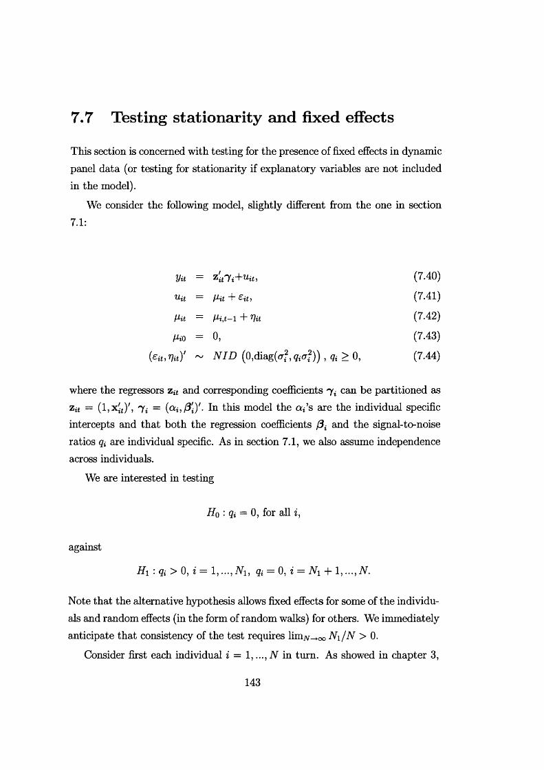
7.7 Testing stationarity and fixed effects

This section is concerned with testing for the presence of fixed effects in dynamic panel data (or testing for stationarity if explanatory variables are not included in the model).

We consider the following model, slightly different from the one in section7.1:

Vit = (7.40)

ttit = (J'it H" &it,

t^it = (J'ij—l " t " Vit (7’ ty

fro = 0, (7.43)

(ea, Vit)' ~ N ID (0,diag(of,&of)) , $ > 0, (7.44)

where the regressors z# and corresponding coefficients can be partitioned as z a = ( l , x j f )', mfi = this model the c^’s are the individual specificintercepts and that both the regression coefficients /3{ and the signal-to-noise ratios ^ are individual specific. As in section 7.1, we also assume independence across individuals.

We are interested in testing

H q : Qi = 0, for all z,

against

Hi : qi > 0 , i = 1,. ..,Ni, $ = 0 , z = Ni + 1, . ..,N.

Note that the alternative hypothesis allows fixed effects for some of the individu­als and random effects (in the form of random walks) for others. We immediately anticipate that consistency of the test requires limN^oo N i /N > 0.

Consider first each individual z = 1,..., N in turn. As showed in chapter 3,

143

section 3.1, the LBI test statistic for H q : qi = 0 against Hi : qi > 0 is given byt / t

f ___ t — 1 \ S=1

t = l

where the uu s are the OLS residuals from regressing yit on zit.The test we propose for our panel data model (7.40)-(7.44) is obtained by

taking the average of the N individual LBI statistics i.e. we consider the statistic

N

(7 -46)i=l

and the test will reject Ho when £ > k, where k is an appropriate critical value. We call this test Average LBI test It is constructed in an analogous maimer to the Average LM test for unit roots proposed by Im, Pesaran, Shin (1997).

If the error terms eit are not white noise (and the regressors are exogenous), we can apply the KPSS correction to £ by replacing Yn=i T u ^ whereQi is a consistent estimator of the long run variance of £u\ see section 3.5. The limiting distribution of the resulting statistic will be unchanged.

In the two subsections below we derive the limiting distribution of £ under Hq first for a model without explanatory variables (test for stationarity) and then with explanatory variables (test for fixed effects). In both cases we have asymp­totic normality. Then in the third subsection below we show the consistency of the test.

Our tests are closely related to the tests of Hadri (1998) and McCoskey and Kao (1998), who consider an LBI test for panel data models where the same variance for the noise and the same signal-to-noise ratio across individuals are assumed4 . The LBI statistic for their model can be derived using theorem 6

of chapter 2 and it is asymptotically equivalent to our statistic £. Then they also propose to use £ to account for heterogeneity in the noise, although they do not prove consistency of the test when only a fraction of the individuals have random effects (in the form of a random walk component).4 McCoskey and Kao (1998) interpret the test as a test for cointegration in panel data.

(7.45)

144

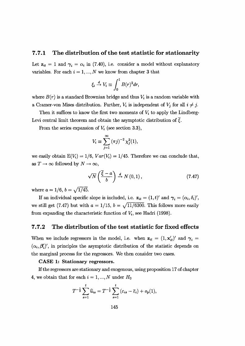
7.7.1 The distribution o f the test statistic for stationarity

Let zn = 1 and tyi = in (7.40), i.e. consider a model without explanatory variables. For each i = 1,..., N we know from chapter 3 that

Z i l V t m C B { r f dr,J o

where B(r) is a standard Brownian bridge and thus Vi is a random variable with a Cramer-von Mises distribution. Further, V* is independent of Vj for all i ^ j.

Then it suffices to know the first two moments of Vi to apply the Lindberg- Levi central limit theorem and obtain the asymptotic distribution of f .

From the series expansion of Vi (see section 3.3),oo

Vi =3 =1

we easily obtain E(V*) = 1/6, Var(Vi) = 1/45. Therefore we can conclude that, as T —► oo followed by N —* oo,

V N N (0,1) , (7.47)

where a = 1/6, b — ^/l/45.If an individual specific slope is included, i.e. za = (1 ,t)' and 7 i = (ai7 ^ )',

we still get (7.47) but with a = 1/15, b = ^11/6300. This follows more easily from expanding the characteristic function of Vi, see Hadri (1998).

7.7.2 The distribution of the test statistic for fixed effects

When we include regressors in the model, i.e. when z it = (1, x 'J ' and 7 i = (a^,/?')', in principles the asymptotic distribution of the statistic depends on the marginal process for the regressors. We then consider two cases.

CASE 1: S ta tionary regressors.If the regressors are stationary and exogenous, using proposition 17 of chapter

4, we obtain that for each i = 1,..., N under H ot t

T ~* Y l ^ ia = T ~^ ^ 2 (£is ~ ^ +S = 1 S = 1

145

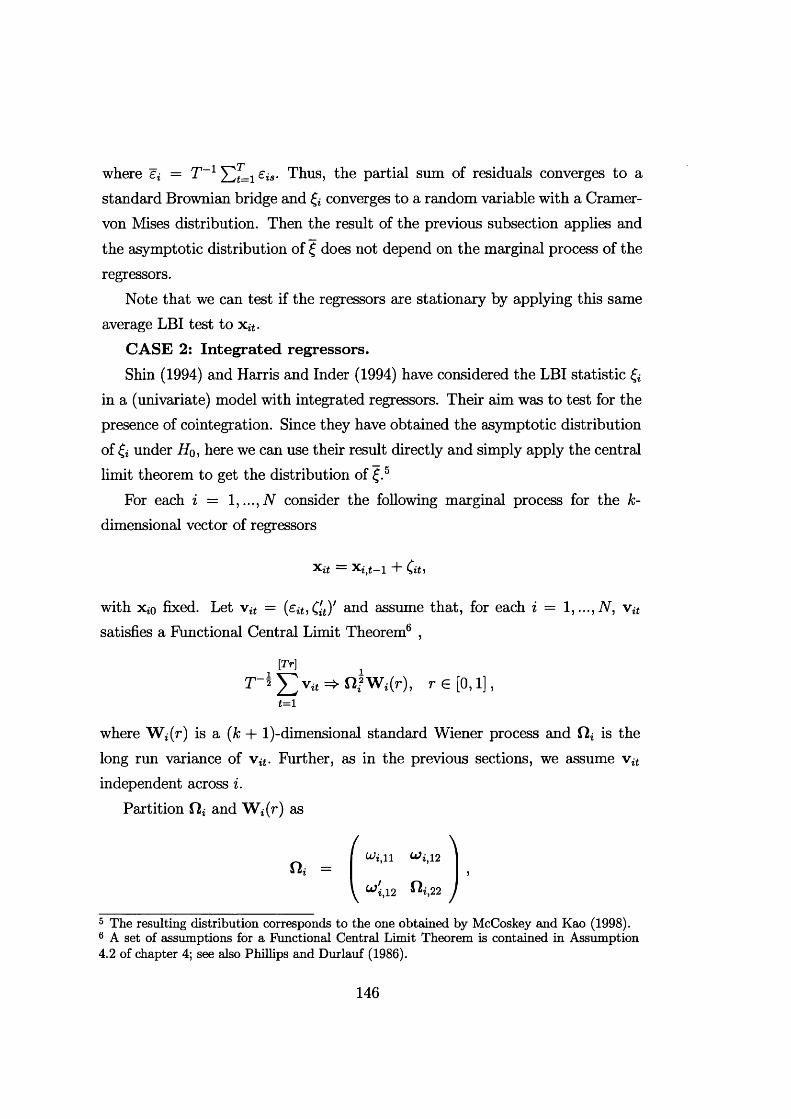
where e* = T _1 £™- Thus, the partial sum of residuals converges to astandard Brownian bridge and £ converges to a random variable with a Cramer- von Mises distribution. Then the result of the previous subsection applies and the asymptotic distribution of £ does not depend on the marginal process of the regressors.

Note that we can test if the regressors are stationary by applying this same average LBI test to x^.

CASE 2: In teg ra ted regressors.Shin (1994) and Harris and Inder (1994) have considered the LBI statistic £*

in a (univariate) model with integrated regressors. Their aim was to test for the presence of cointegration. Since they have obtained the asymptotic distribution of £j under Hq, here we can use their result directly and simply apply the central limit theorem to get the distribution of £.5

For each i = 1 consider the following marginal process for the k-dimensional vector of regressors

xa — + C,n,

with Xio fixed. Let v it = {£it,CitY an(i assume that, for each i = 1 v itsatisfies a Functional Central Limit Theorem6 ,

[T r ] i

r - ^ v a ^ n f W i t r ) , r e [0 , 1],t=1

where W j(r) is a (k + l)-dimensional standard Wiener process and is the long run variance of v it. Further, as in the previous sections, we assume v it independent across i.

Partition and W j(r) as

ft; =(

11 &i, 12

y wi,12 *>22

5 The resulting distribution corresponds to the one obtained by McCoskey and Kao (1998).6 A set of assumptions for a Functional Central Limit Theorem is contained in Assumption 4.2 of chapter 4; see also Phillips and Durlauf (1986).

146

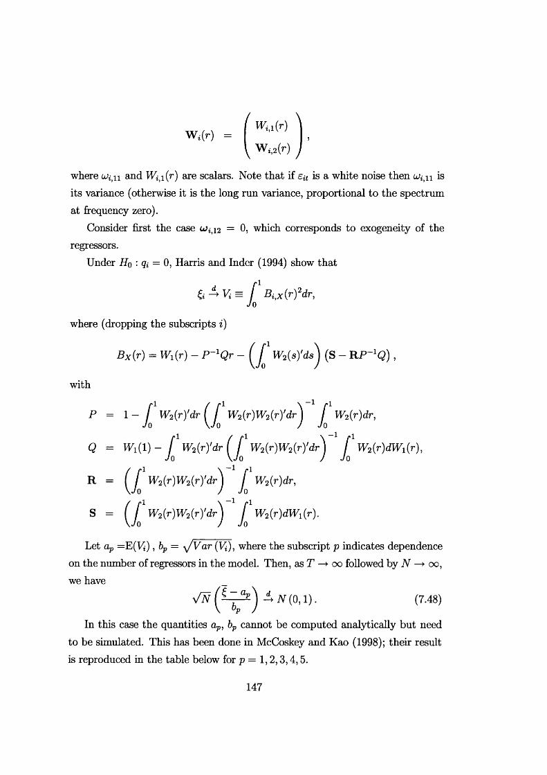
Wj(r) =1 Wi, i(r) N

Wy(r) )where u^n and W^i(r) are scalars. Note that if en is a white noise then lj u is its variance (otherwise it is the long run variance, proportional to the spectrum at frequency zero).

Consider first the case 0^12 = 0, which corresponds to exogeneity of the regressors.

Under H q : ^ = 0, Harris and Inder (1994) show that

Vj = f B<x(rfdr,Jo

where (dropping the subscripts i)

B x(r) = WAr) - P ^ Q r - ( j f W2(s)'ds) (S - R P ^ Q ) ,

with

P =

Q =

R =

S =

1 _ L W2^ ' d r ( J 0 W2(r)W2(r)'dr\ £ W2(r)dr,

WAO - £ W2(r)’dr Q f W2(r)W2(r)'dr\ £ W2(r)dWAr),

( / W2(.r )W‘2(r )'dr n : W2(r)dr,

( L Jg W 2( r ) d W i( r ) .

Let ap = E ( V i ) , bp = y/Var (Vi), where the subscript p indicates dependence on the number of regressors in the model. Then, as T —► 00 followed by N —> 00 , we have _

y/N ^ N (0,1). (7.48)

In this case the quantities ap, bp cannot be computed analytically but needto be simulated. This has been done in McCoskey and Kao (1998); their resultis reproduced in the table below for p = 1, 2 ,3,4,5.

147

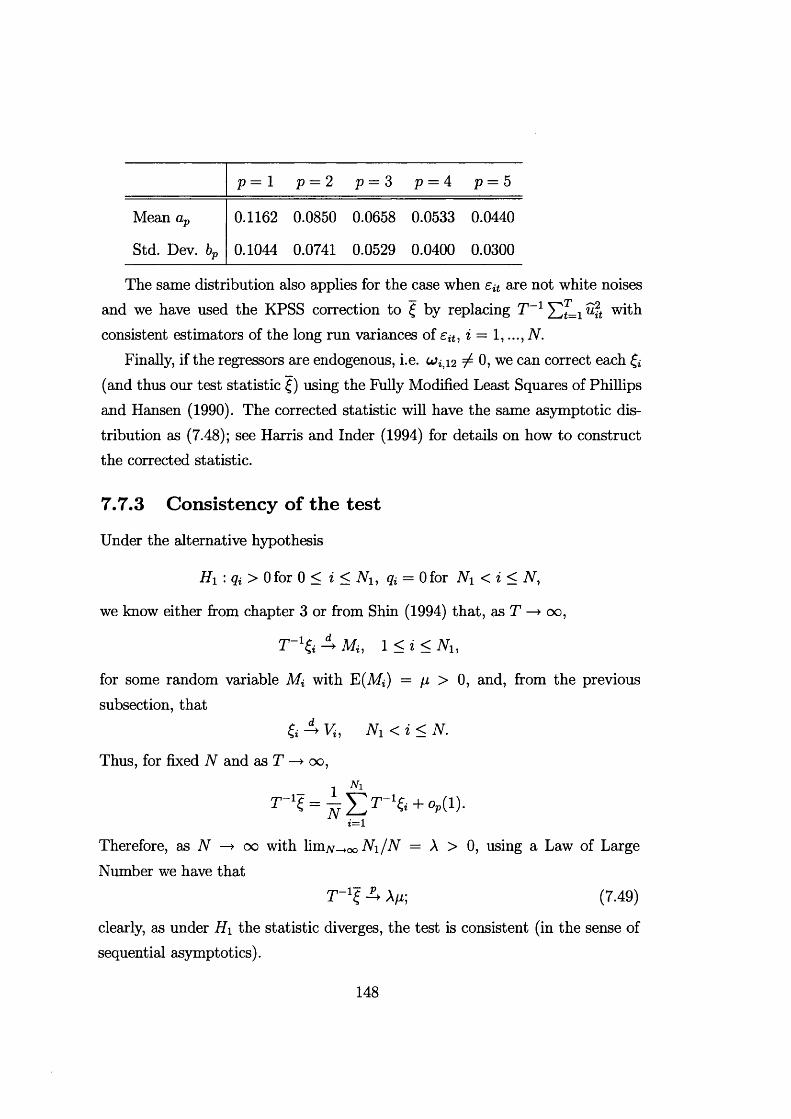
p = 1 p = 2 p = 3 p = 4 p = 5

Mean ap 0.1162 0.0850 0.0658 0.0533 0.0440

Std. Dev. bp 0.1044 0.0741 0.0529 0.0400 0.0300

The same distribution also applies for the case when eit are not white noisesand we have used the KPSS correction to £ by replacing T~l Ylt=i ™it withconsistent estimators of the long run variances of eit, i = 1 , N.

Finally, if the regressors are endogenous, i.e. 0^12 7 0, we can correct each £* (and thus our test statistic £) using the Fully Modified Least Squares of Phillips and Hansen (1990). The corrected statistic will have the same asymptotic dis­tribution as (7.48); see Harris and Inder (1994) for details on how to construct the corrected statistic.

7.7.3 Consistency o f the test

Under the alternative hypothesis

H1 :qi > Ofor 0 < i < N\, Qi = 0 for Ni < i < N,

we know either from chapter 3 or from Shin (1994) that, as T —» 00,

l < i < N u

for some random variable Af< with E (Mi) = p, > 0 , and, from the previous subsection, that

6 ± V i , N i < i < N.

Thus, for fixed N and as T —> 00 ,

1 NlT " 1£ = v £ r " 16 + o »(1)-

i=1

Therefore, as N —> 00 with lini/v->oo N i/N = A > 0, using a Law of Large Number we have that

T - 1? A A/t; (7.49)

clearly, as under Hi the statistic diverges, the test is consistent (in the sense of sequential asymptotics).

148

7.8 Illustration: estim ating a production func­tion from a panel of US manufacturing firms

In this section we use model (7.1)-(7.5) to estimate a Cobb-Douglas production function for a balanced panel of 404 R&D manifacturing companies observed for 12 years, 1978-1989. These data are a subset of a dataset constructed by Bron- wyn Hall (and available at her homepage at Berkeley University). Similar data have been used by Blundell and Bond (1999) to estimate a production function in the autoregressive framework. Further details on the data constructions are in Mairesse and Hall (1996).

The dependent variables is sales, as a proxy for output, and the regressors are capital stock and employment, measured at the end of the firm’s accounting year. The data are in logarithms and a time component common to all individuals has been subtracted from the outset, as suggested in section 7.6.

Let nit, kit be respectively the labour and the capital input for firm i at time t. We have considered two specifications of the production function, corresponding to (7.1)-(7.5) with xn = {nit,k it)' and x it = (nit, 77,i|t_i, kiu fc^t-i)' respectively. The two models, labelled model 1 and model 2, have been estimated by MLE with heterogeneous variance of the noise (i.e. of unrestricted across firms), by MLE with homogeneous variance of the noise, and by OLS in first differences. The estimation results are reported in the tables below, where within brackets are contained either the t-statistics for the regression coefficients or the p-values for the tests. Note the starred coefficients in the tables, which are averages across individuals.

From the t-statistics of model 2 we immediately see that we cannot exclude lagged values of the regressors, so model 1 is misspecified. We have also tried to use more lags, without statistical significance. So model 2 seems the appropriate one.

149

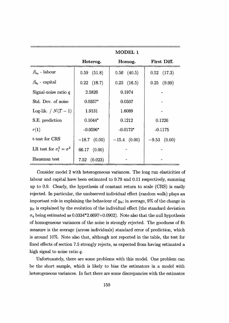
H eterog.

M ODEL 1

Homog. F irs t Diff.

j3nt - labour 0.59 (51.8) 0.56 (40.5) 0.52 (17.3)

/3kt - capital 0.22 (18.7) 0.25 (16.5) 0.25 (9.99)

Signal-noise ratio q 2.5826 0.1974 -

Std. Dev. of noise 0.0357* 0.0507 -

Log-lik. / N (T - 1) 1.9131 1.6089 -

S.E. prediction 0.1044* 0.1212 0.1226

r(l) -0.0596* -0.0173* -0.1175

t-test for CRS -18.7 (0.00) -15.4 (0.00) -9.53 (0.00)

LR test for of = a2 66.17 (0.00) - -

Hausman test 7.52 (0.023) - -

Consider model 2 with heterogeneous variances. The long run elasticities of labour and capital have been estimated to 0.79 and 0.11 respectively, summing up to 0.9. Clearly, the hypothesis of constant return to scale (CRS) is easily rejected. In particular, the unobserved individual effect (random walk) plays an important role in explaining the behaviour of yu; in average, 9% of the change in yit is explained by the evolution of the individual effect (the standard deviation ctv being estimated as 0.0334*2.6697=0.0902). Note also that the null hypothesis of homogeneous variances of the noise is strongly rejected. The goodness of fit measure is the average (across individuals) standard error of prediction, which is around 10%. Note also that, although not reported in the table, the test for fixed effects of section 7.5 strongly rejects, as expected from having estimated a high signal to noise ratio q.

Unfortunately, there are some problems with this model. One problem can be the short sample, which is likely to bias the estimators in a model with heterogeneous variances. In fact there are some discrepancies with the estimates

150

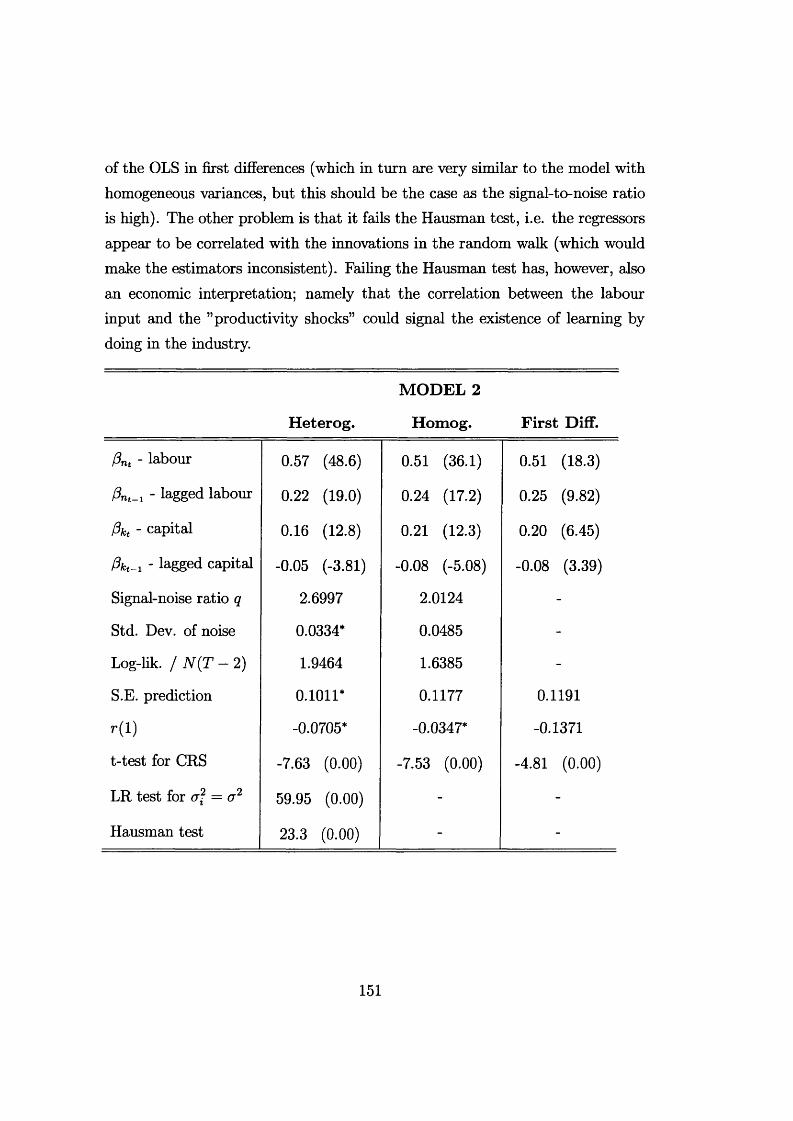
of the OLS in first differences (which in turn are very similar to the model with homogeneous variances, but this should be the case as the signal-to-noise ratio is high). The other problem is that it fails the Hausman test, i.e. the regressors appear to be correlated with the innovations in the random walk (which would make the estimators inconsistent). Failing the Hausman test has, however, also an economic interpretation; namely that the correlation between the labour input and the ’’productivity shocks” could signal the existence of learning by doing in the industry.

H eterog.

M ODEL 2

Homog. F irs t Diff.

Pnt - labour 0.57 (48.6) 0.51 (36.1) 0.51 (18.3)

/?nt-1 - lagged labour 0.22 (19.0) 0.24 (17.2) 0.25 (9.82)

Pkt - capital 0.16 (12.8) 0.21 (12.3) 0.20 (6.45)

Pkt-i - lagged capital -0.05 (-3.81) -0.08 (-5.08) -0.08 (3.39)

Signal-noise ratio q 2.6997 2.0124 -

Std. Dev. of noise 0.0334* 0.0485 -

Log-lik. / N (T - 2) 1.9464 1.6385 -

S.E. prediction 0 .1011* 0.1177 0.1191

r(l) -0.0705* -0.0347* -0.1371

t-test for CRS -7.63 (0.00) -7.53 (0.00) -4.81 (0.00)

LR test for erf = er2 59.95 (0.00) - -

Hausman test 23.3 (0.00) - -

151

REFERENCES

Ahn, S.C. and P: Schmidt (1995), Efficient estimation of models for dy­namic panel data, Journal of Econometrics 68 , 5-28.

Ahn, S.C. and P: Schmidt (1997), Efficient estimation of dynamic panel data models: alternative assumptions and simplified estimation, Journal of Econometrics 76, 309-321.

Anderson, T.W. and D.A. Darling (1952), Asymptotic theory of certain ’Goodness of F it’ criteria based on stochastic processes, Annals of Math­ematical Statistics 23, 193-212.

Andrews, D.J. (1991), Heteroskedasticity and autocorrelation consistent covariance matrix estimation, Econometrica, 59, 817-858.

Andrews, D.W.K. and J.C. Monahan (1992). An improved heteroscedas- ticity and autocorrelation consistent covariance matrix estimation. Econo­metrica 60, 953-66.

Ansley, C.F. and R. Kohn (1985), Estimation, filtering and smoothing in state space models with incompletely specified initial conditions, Annals of Statistics 13, 1286-1316.

Arellano, M. and S. Bond (1991), Some tests of specification for panel data; Monte Carlo evidence and an application to employment equation, Review of Economic Studies 58, 277-297.

Bai, J. (1994), Least squares estimation of a shift in linear processes, Jour­nal of Time Series Analysis 15, 453-472.

Bai, J. (1997), Estimation of a change point in multiple regression models, Review of Economics and Statistics, 551-563.

Balcombe, K. (1999), Seasonal unit root tests with structural breaks in deterministic seasonality, Oxford Bulletin of Economics and Statistics 61, 569-595.

Banerjee, A., Lumsdaine, R.L. and J.H. Stock (1992), Recursive and se­quential tests of the unit root and trend break hypothesis: theory and international evidence, Journal of Business and Economic Statistics 10, 271-287.

Blundell, R. and S. Bond (1998), Initial conditions and moment restrictions in dynamic panel data models, Journal of econometrics 87, 115-143.

152

Blundell, R. and S. Bond (1999), GMM estimation with persistent panel data: an application to production function estimation, IFS Working Pa­per W99/4.

Blundell, R., Bond, S. and F. Windmeijer (1999), Estimation of dynamic panel data models: improving on the performance of the standard GMM estimators, IFS Working Paper WOO/12.

Box, G.E.P. and G.M. Jenkins (1976), Time series analysis, forecasting and control, San Francisco, Holden-Day.

Caner, M. (1998), A locally optimal seasonal unit root test. Journal of Business and Economic Statistics, 16, 349-56.

Canova, F. and B.E. Hansen (1995), Are seasonal patterns constant over time? A test for seasonal stability, Journal of Business and Economic Statistics, 2 , 292-349.

Chan, N.H. and C.Z. Wei (1988), Limiting distributions of least squares estimates of unstable autoregressive processes, Annals of Statistics 16, 367- 401.

Choi, I. and B.C. Ahn (1995), Testing for cointegration in systems of equations, Econometric Theory 11, 952-983.

Cleveland, W.S. and S.J Devlin (1980), Calendar effects in monthly time series: detection by spectrum and graphical methods. Journal of the Amer­ican Statistical Association, 75, 487-96.

Davidson (1999), When is a time series 1(0)? Evaluating the memory properties of nonlinear dynamic models, mimeo.

de Jong, P. (1988), The likelihood for a state space model, Biometrika 75, 165-169.

de Jong, P. (1991), The diffuse Kalman filter, Annals of Statistics 19, 1073-1082.

de Jong, P. and J. Penzer (1998), Diagnosing shocks in time series. Journal of the American Statistical Association, 93 :796-806.

Dickey, D.A. and W.A. Fuller (1979), Distribution of the estimators for autoregressive time series with a unit root, Journal of the American Sta­tistical Association 74, 427-431.

153

Dickey, D.A. and W.A. Fuller (1981), Likelihood ratio statistics for au­toregressive time series with a unit root, Econometrica, 1057-1072.

Doornik, J.A. (1998), Object-oriented matrix programming using Ox 2.0, Timberlake Consultants Press, New York.

Engle, R.F. and C.W.J. Granger (1987), Co-integration and error correc­tion: representation, estimation and testing, Econometrica 55, 251-276.

Engle, R.F. and B.S. Yoo (1991), Cointegrated economic time series: an overview with new results, in Engle, R.F. and C.W.J. Granger (eds.), Long Run Economic Relationships: Readings in Cointegration. Advanced Text in Econometrics, Oxford University Press, Oxford, 237-266.

Ferguson, T.S. (1969), Mathematical Statistics: a decision theoretic ap­proach, Academic Press, New York.

Franses, P.H. and T.J. Vogelsang (1998), On seasonal cycles, unit roots, and mean shifts, The Review of Economics and Statistics 80, 231-240.

Gardner, L.A. (1969), On detecting changes in the mean of normal variates, Annals of Mathematical Statistics 40, 116-126.

Gikhman, I.I. and A.V. Skorokhod (1975), The theory of stochastic processes (translated from the Russian by S. Kotz). Berlin: Springer- Verlag.

Giri, N.C. (1996), Multivariate statistical analysis, Dekker, New York.

Gregory, A.W. and B.E. Hansen (1996a), Residual based tests for cointe­gration in models with regime shifts, Journal of Econometrics 70, 99-126.

Gregory, A.W. and B.E. Hansen (1996b), Tests for cointegration in models with regime and trend shifts, Oxford Bulletin of Economics and Statistics 58, 555-560.

Hao, K. (1996), Testing for structural change in cointegrated regression models: some comparisons and generalizations, Econometric Reviews 15, 401-429.

Hadri, J. (1998), Testing for stationarity in heterogeneous panel data, mimeo.

Harris, D. and B. Inder (1994), A test of the null hypothesis of cointe­gration, in Nonstationary Time Series Analysis and Cointegration, Harg­reaves, Colin P., ed., Oxford University Press, New York.

154

Harvey, A.C. (1989), Forecasting, structural time series models and the Kalman filter, Cambridge, Cambridge University Press.

Harvey, A.C. and J. Durbin (1986), The effect of seat belt legislation on British road casualties: a case study in structural time series modelling, Journal of the Royal Statistical Society, Series A 149, 187-227.

Harvey, A.C. and A. Jaeger (1993), Detrending, stylized facts and the business cycle, Journal of Applied Econometrics 8 , 231-247.

Harvey, A.C. and J. Bernstein (2000), Measurement and testing of inequal­ity from time series of deciles with an application to US wages. Mimeo.

Harvey, A.C. and S.J. Koopman (1992), Diagnostic checking of unobserved components time series models, Journal of Business and Economics Sta­tistics 10, 377-389.

Harvey, A.C. and S.J. Koopman (1996), Structural time series models in medicine, Statistical Methods in Medical Research, 23-49.

Harvey, A.C. and S.J. Koopman (1997), Multivariate structural time series models, in System Dynamics in Economic and Financial Models, C. Heij, J.M. Schumacher, B. Hanzon and C. Praagman editors, New York, John Wiley and Sons.

Harvey, A.C., Koopman, S.J. and J. Penzer (1998), Messy time series, In T.B. Folby and R.C. Hill (eds.), Advances in Econometrics, Volume 13, JAI Press, New York.

Harvey, A.C., Ruiz, E. and N. Shepard (1994), Multivariate stochastic variance models, Review of Economic Studies 61, 247-264.

Harvey, A.C. and M. Streibel (1997), Testing for nonstationary unobserved components, mimeo.

Hobijn, B. and P.H.Franses (2000), Asymptotically perfect and relative convergence of productivity, Journal of Applied Econometrics, 15, 59-81.

Hsiao, C. (1986), Analysis of panel data, Cambridge University Press, Cambridge.

Hylleberg, S., Engle, R.F., Granger, C.W.J. and B.S. Yoo (1990), Seasonal integration and cointegration, Journal of Econometrics 99, 215-238.

Im, K., Pesaran, H. and Y. Shin (1997), Testing for unit roots in hetero­geneous panels, mimeo.

155

Inoue, A. (1999), Test of cointegrating rank with a trend-break, Journal of Econometrics 90, 215-237.

Johansen, S. (1988), Statistical analysis of cointegration vectors, Journal of Economic Dynamics and Control 12, 131-154.

Johansen, S. (1991), Estimation and hypothesis testing of cointegration vectors in Gaussian vector autoregressive model, Econometrica 59, 1551- 1580.

Johansen, S. (1995), Likelihood-based inference in cointegrated vector au­toregressive models, Oxford University Press, Oxford.

Kao, C. (1999), Spurious regression and residual-based tests for cointegra­tion in panel data, Journal of Econometrics 90, 1-44.

Kariya, T. (1980), Locally robust tests for serial correlation in least squares regression, Annals of Statistics 6 , 1065-1070.

King, M.L. (1980), Robust tests for spherical symmetry and their applica­tion to least squares regressions, Annals of Statistics 8 , 1265-1271.

King, M.L. and G.H. Hillier (1985), Locally best invariant tests of the error covariance matrix in the linear regression model, Journal of the Royal Statistical Society, Series B 47, 98-102.

Kitagawa, G., and W Gersch. Smoothness priors analysis of time series. Berlin: Springer-Verlag (1996).

Koopman, S.J. (1997), Exact initial Kalman filtering and smoothing for nonstationary time series models, Journal of the American Statistical As­sociation 92, 1630-1638.

Koopman, S.J. and A.C. Harvey (1999), Computing observation weights for signal extraction and filtering, mimeo.

Koopman, S.J., Shepard, N. and J.A. Doornik (1998), Statistical algo­rithms for models in state space using SsfPack 2.2, Econometrics Journal 1, 1-55.

Koopman, S.J., Harvey, A.C., Doornik J.A. and N. Shephard (1995), STAMP 5.0 Structural time series analyser, modeller and predictor. Lon­don: Chapman and Hall.

156

Kunimoto, N. (1996), Structural changes, unit roots, cointegration hy­potheses with an application to macro time series. Kinyu Kenkyu, Institute of Monetary and Economic Studies, Bank of Japan 15 (5), 1-43.

Kwiatkowski, D., Phillips, P.C.B., Schmidt, P. and Y. Shin (1992), Testing the null hypothesis of stationarity against the alternative of a unit root: how sure are we that economic time series have a unit root?, Journal of Econometrics 44, 159-178.

Lancaster, T. (2000), The incidental parameter problem since 1948, Jour­nal of Econometrics 95, 391-413.

Lee, J. (1996). On the power of stationarity tests using optimal bandwidth estimates. Economics Letters, 51, 131-7.

Lee, D. and P. Schmidt (1996), On the power of the KPSS test against fractionally integrated alternatives. Journal of Econometrics 73, 285-302.

Lee, J., Huang, C.J. and Y. Shin (1997), On stationary tests in the presence of structural breaks, Economics Letters 55, 165-172.

Lehmann, E.L. (1959), Testing statistical hypotheses, New York, Wiley.

Leybourne, S.J. and B.P.M. McCabe (1994), A consistent test for a unit root, Journal of Business and Economic Statistics 12, 157-166.

Leybourne, S.J., Mills, T.C. and P. Newbold (1999), Spurious rejections by Dickey-Fuller tests in the presence of a break under the null, Journal of Econometrics 87, 191-203.

Lopes, A.S. and A. Montanes (1998), The asymptotic and finite sample behaviour of seasonal unit roots tests under the presence of a break in the deterministic seasonal pattern, mimeo.

MacNeill, I. (1978), Properties of sequences of partial sums of polynomial regression residuals with applications to tests for change of regression at unknown times, Annals of Statistics 6 , 422-433.

Mairesse, J. and B.H. Hall (1996), Estimating the productivity of research and development in French and US manufacturing firms: an exploration of simultaneity issues with GMM methods, in Wagner, K. and B. Van Ark (eds.), International productivity differences and their explanations, Elsevier Science, 285-315.

McCoskey, S. and C. Kao (1998), A residual based test of the null of cointegration in panel data, Econometric Review 17, 57-84.

157

Marshall, P. (1992), Estimating time-dependent means in dynamic models for cross-section of time series, Empirical Economics 17, 25-33.

Nabeya, S. and K. Tanaka (1988), Asymptotic theory of a test for the constancy of regression coefficients against the random walk alternative, Annals of Statistics 16, 218-235.

Nelson, C.R. and C.I. Plosser (1982), Trends versus random walks in macroeconomic time series: some evidence and implications, Journal of Monetary Economics 10, 139-162.

Neyman, J. and E.L. Scott (1948), Consistent estimates based on partially consistent observations, Econometrica 16, 1-32.

Nickell, S. (1981), Biases in dynamic models with fixed effects, Economet­rica 49, 1417-1426.

Nyblom, J. (1986), Testing for deterministic linear trend in time series, Journal of the American Statistical Association 81, 545-549.

Nyblom, J. (1989), Testing for the constancy of parameters over time, Journal of the American Statistical Association 84, 223-230.

Nyblom, J. and A.C. Harvey (1997), Tests against smooth stochastic trends, mimeo.

Nyblom, J. and A.C. Harvey (2000), Tests of common trends, Econometric Theory 16, forthcoming.

Nyblom, J. and T. Makelainen (1983), Comparison of tests for the pres­ence of random walk coefficients in a simple linear model, Journal of the American Statistical Association 78, 856-864.

Perron, P. (1989), The Great Crash, the oil price shock, and the unit root hypothesis, Econometrica 57, 1361-1401.

Perron, P. and T.J. Vogelsang (1992a), Nonstationarity and level shifts with an application to Purchasing Power Parity, Journal of Business and Economic Statistics 10, 301-320.

Perron, P. and T.J. Vogelsang (1992b), Testing for a unit root in a time se­ries with a changing mean: corrections and extensions, Journal of Business and Economic Statistics 10, 467-470.

Pesaran, M.H. and Y. Shin (1995), Long run structural modeling, Univer­sity of Cambridge Department of Applied Economics Working Paper.

158

Phillips, P.C.B. (1987), Time series regression with a unit root, Economet­rica 55, 277-301.

Phillips, P.C.B. (1991), Optimal inference in cointegrated systems, Econo­metrica 59, 283-306.

Phillips, P.C.B. (1994), Some exact distribution theory for maximum like­lihood estimators of cointegrating coefficients in error correction models, Econometrica 62, 73-93.

Phillips, P.C.B and S.N. Durlauf (1986), Multiple time series regressions with integrated processes, Review of Economic Studies 53, 473-95.

Phillips, P.C.B. and B. Hansen (1990), Statistical inference in instrumental variables regression with 1(1) processes, Review of Economic Studies 53, 473-495.

Phillips, P.C.B. and H.R. Moon (2000), Linear regression limit theory for nonstationary panel data, Econometrica, forthcoming.

Phillips, P.C.B. and S. Ouliaris (1990), Asymptotic properties of residual based tests for cointegration, Econometrica 58, 165-194.

Phillips, P.C.B. and P. Perron (1988), Testing for a unit root in time series regression, Biometrika 75, 335-346.

Phillips, P.C.B and V. Solo (1992), Asymptotics for linear processes, An­nals of Statistics 20, 971-1001.

Phillips, P.C.B. and Z. Xiao (1998), A primer on unit root testing, mimeo.

Proietti, T. (1998), Seasonal heteroscedasticity and trends, Journal of Forecasting, 17, 1-17.

Proietti, T. (2000). Comparing seasonal components for structural time series models, International Journal of Forecasting, 16, 247-60.

Rao, C.R. (1973), Linear statistical inference and its applications, 2nd ed., Wiley, New York.

Said, S. and D.A. Dickey (1984), Testing for unit roots in autoregressive moving average models of unknown order, Biometrika 71, 599-608.

Shephard, N.G. (1993), Maximum likelihood estimator of regression mod­els with stochastic trend components, Journal of the American Statistical Association 88 , 590-595.

159

Shephard, N.G. and A.C. Harvey (1990), On the probability of estimating a deterministic component in the local level model, Journal of Time Series Analisys 11, 339-347.

Shin, Y. (1994), A residual based test of the null of cointegration against the alternative of no cointegration, Econometric Theory 10, 91-115.

Smith, J. and J. Otero (1997), Structural breaks and seasonal integration, Economics Letters 56, 13-19.

Smith, R.J. and A.M.R. Taylor (1998), Additional critical values and as­ymptotic representations for seasonal unit root tests, Journal of Econo­metrics 85, 269-288.

Soukup, R.J. and D.F. Findlay (2000), On the spectrum diagnostics used by X-12- ARIMA to indicate the presence of trading day effects after modeling or adjustment, @ 1999 Proceedings of the Business and Economic Statistics Section, American Statistical Association, 144-149.

Taylor, A.M.R.(2000), Locally optimal tests against seasonal unit roots. University of Birmingham discussion paper, 99-12

White (1980), An heteroskedasticity-consistent covariance matrix estima­tor and a direct test for heteroskedasticity, Econometrica 48, 817-838.

Young, P., Recursive estimation and time series analysis. Berlin: Springer- verlag (1984).

Zivot, E. and D.W.K. Andrews (1992), Further evidence on the Great Crash, the oil-price shock, and the unit-root hypothesis, Journal of Busi­ness and Economic Statistics 10, 251-270.

160