testing and extending the capital asset pricing model
TRANSCRIPT

Testing and Extending the Capital Asset
Pricing Model
Gabriel Koh, Diana Kleinknecht, Paolo Parziano, Lei Peng
IB9Y8 Asset Pricing Group 14
MSc Finance
List of Contents
Abstract ................................................................................................................................................... 1
Introduction ............................................................................................................................................. 1
Literature Review .................................................................................................................................... 2
Data Description ...................................................................................................................................... 3
Methodology ........................................................................................................................................... 3
Two-Stage Regression ......................................................................................................................... 3
Rolling Window Regression ................................................................................................................. 4
Jarque-Bera Normality Test ................................................................................................................. 5
Testing of Pricing in Idiosyncratic Risk ................................................................................................ 5
Testing of Linearity in CAPM ............................................................................................................... 6
Wald test ............................................................................................................................................. 6
Gibbons, Ross, and Shanken test ........................................................................................................ 7
Empirical Results ..................................................................................................................................... 8
Testing the Capital Asset Pricing Model (CAPM) ................................................................................. 8
Finding Anomalies in the CAPM .......................................................................................................... 9
Explanatory Power of Risk Factors .................................................................................................... 10
Correlation between Pricing Errors and Firm Characteristics ........................................................... 12
Building and Testing “Factor-Mimicking Portfolios” ......................................................................... 13
Caveats and Limitations ........................................................................................................................ 15
Conclusion ............................................................................................................................................. 16
References ............................................................................................................................................. 17
IB9Y8 Asset Pricing Group 14
MSc Finance 1
Abstract
This paper attempts to prove whether the conventional Capital Asset Pricing Model (CAPM)
holds with respect to a set of asset returns. Starting with the Fama-Macbeth cross-sectional
regression, we prove through the significance of pricing errors that the CAPM does not hold.
Hence, we expand the original CAPM by including risk factors and factor-mimicking portfolios
built on firm-specific characteristics and test for their significance in the model. Ultimately, by
adding significant factors, we find that the model helps to better explain asset returns, but
does still not entirely capture pricing errors.
Introduction
A central economic, but still not completely answered question in the field of finance, is why
different assets earn substantially different returns on average. In this paper, we empirically
examine a given set of data in the context of different aspects of asset pricing theory. Based
on the given data, we first apply a two-stage regression approach (Cochrane, 2001), as well
as the Fama-MacBeth rolling window procedure (1973), to test for the validity of the Capital
Asset Pricing Model (CAPM). We find that assets have an inherent pricing error (𝛼𝑘 ≠ 0) and
that there exists a risk premium which is not explained by the market. Additionally, we find that
idiosyncratic risk is not priced and that the CAPM is indeed linear. In order to improve the
explanatory power of the cross-section of returns and hence reduce pricing errors, we
individually test the significance of two additional risk factors. We then regress the pricing
errors on two anonymous firm characteristics and create a factor-mimicking portfolio for the
significant characteristic.
From our results, we find that although the one risk factor and factor-mimicking portfolio are
significant in explaining pricing errors, the Gibbons, Ross and Shanken (GRS) test shows that
the pricing errors are still jointly not equal to zero.
The paper is organised as follows. First, we conduct a brief literature review with respect to the
development of asset pricing models. In the following, we give a comprehensive description of
the data, methodology, and empirical results. Finally, we evaluate our paper by discussing
some of the caveats and limitations.
IB9Y8 Asset Pricing Group 14
MSc Finance 2
Literature Review
Sharpe (1964) and Lintner (1965) were the first to develop the CAPM, which marks the
beginning of asset pricing theory. The CAPM builds on the model of portfolio choice as
suggested by Markowitz (1959). This model assumes investors to be risk averse and
consequently investors only choose mean-variance-efficient portfolios. Building on this
assumption, Sharpe (1964) states that in equilibrium, if all investors act rationally, assets can
be priced by only considering a market risk factor in the model. The risk premium earned by
an asset is proportional to the asset’s exposure to systematic risk, which is captured by the
asset’s market beta. Idiosyncratic or firm specific risk should not be priced as it can be
eliminated by holding a well-diversified portfolio. However, the literature finds evidence of the
existence of a pricing-error in the model, the so called Jensen’s Alpha (Jensen, 1968). The
pricing error is defined as the difference between the realised return of a stock and its predicted
return according to the CAPM. If the model holds, one would expect the average pricing errors
across assets to be zero, which is often not the case (Harvey, 1988).
Assuming that the market risk premium alone cannot sufficiently capture variations in asset
returns, and acknowledging the presence of anomalies in the CAPM, other researchers
extended the original CAPM model by adding various factors into the model. Basu (1977) finds
evidence that future returns on stocks with high P/E ratio are higher than predicted by the
CAPM, when sorted on their P/E ratio.
Fama and French (1993) accounts for size, book-to-market ratio, leverage and earnings-to-
price ratio in their model. They find that size and book-to-market (B/M) help to better explain
the cross-section of average returns. Banz (1981) also finds that average returns on small
stocks are higher. Furthermore, Rosenberg, Reid and Lanstein (1985), as well as Stattman
(1980) conclude that stocks with high B/M ratio earn higher premiums.
Stemming from the work of Hendricks, Patel & Zeckhauser (1993), Carhart (1997) added a
fourth factor, the so called momentum factor, to the Fama-French three-factor model. The
factor is constructed by forming diversified portfolios that long “winner” and short “loser” stocks.
In their most recent model, Fama and French (2015) extend their three-factor model to a five-
factor model, including a factor that accounts for the profitability and investment level of a firm.
Their results show that high operating profitability and high investments explain excess returns.
Hou, Xue and Zhang (2015) find similar results. According to them, a model which includes
IB9Y8 Asset Pricing Group 14
MSc Finance 3
the market factor, a size factor, a profitability factor, as well as an investment factor improve
the model in capturing anomalies of the CAPM than the Fama-French three-factor model.
As shown above, there exists a great amount of literature which provides evidence that the
original CAPM might not be the best model to explain the cross-section of expected returns,
and factors other than systematic risk might affect asset pricing.
Data Description
The data set used for the analysis in this paper contains monthly returns on the stock prices
of 50 firms for a sample period of 20 years, which adds up to a total of 12,000 observations. In
this paper, we assume that the stock prices are stationary, therefore there should not be any
spurious regression.
The market return for each period is calculated using an equally weighted portfolio of the 50
assets. In addition to the returns for each of the 50 firms, two firm-specific characteristics, are
taken into consideration. These two characteristics vary not only in the cross-section, but they
are also time-varying for each firm. Moreover, the analysis takes monthly observations for two
risk factors into account. These risk factors are considered to be seen as returns on portfolios
or trading strategies.
Methodology
Two-Stage Regression
To effectively estimate the efficiency of the CAPM model, we start running the two-stage
regression to test the CAPM (Fama and Macbeth, 1973), which we will use throughout this
report. Our procedure starts by regressing the returns of assets on market returns to obtain
the individual estimates of each asset.
𝑅𝑒𝑡𝑢𝑟𝑛𝑡,𝑘 − 𝑅𝑖𝑠𝑘𝑓𝑟𝑒𝑒 = 𝛼𝑘 + 𝛽𝑘𝑚(𝑀𝑎𝑟𝑘𝑒𝑡𝑅𝑒𝑡𝑢𝑟𝑛𝑡 − 𝑅𝑖𝑠𝑘𝑓𝑟𝑒𝑒) + 𝜖𝑡,𝑘 (𝐻1)
Where:
𝑅𝑒𝑡𝑢𝑟𝑛𝑡,𝑘 - Return on asset k in period t
𝑅𝑖𝑠𝑘𝑓𝑟𝑒𝑒 - Risk-free rate
𝛼𝑘: - Constant term
𝛽𝑘𝑚: - Factor loading of market portfolio
𝑀𝑎𝑟𝑘𝑒𝑡𝑅𝑒𝑡𝑢𝑟𝑛𝑡 - Market return in period t
𝜖𝑡: - Residual terms in period t
IB9Y8 Asset Pricing Group 14
MSc Finance 4
Given that the risk-free rate is zero in our analysis (as specified in the task), we can modify the
model:
𝑅𝑒𝑡𝑢𝑟𝑛𝑡,𝑘 = 𝛼𝑘 + 𝛽𝑘𝑚𝑀𝑎𝑟𝑘𝑒𝑡𝑅𝑒𝑡𝑢𝑟𝑛𝑡 + 𝜖𝑡,𝑘 (𝐻2)
Furthermore, we assume that residuals are:
1. Uncorrelated across assets and hence, cov(𝜖𝑗, 𝜖𝑘) = 0, for j ≠ k
2. Uncorrelated with factors and hence, 𝑐𝑜𝑣(𝐹𝑗 , 𝜖𝑘) = 0, ∀ j and k.
The first stage of the two-stage regression is a time-series regression. We run the time series
by regressing each of our 50 assets from month 1 to 240 on the market portfolio. From this we
will obtain a set of 50 estimates of alpha (�̂�𝑘) and beta (�̂�𝑘𝑚) which captures the sensitivity of
asset return to monthly changes in the market portfolio.
Next, by regressing the average asset returns (i.e. �̂�𝑘 =1
𝑇∑ 𝑅𝑒𝑡𝑢𝑟𝑛𝑘,𝑡
𝑇𝑡=1 ) on the betas of the
market (H3), we obtain the estimates of the gamma values (𝛾0 & �̂�1) which are the average
pricing error and the market risk premium respectively.
�̂�𝑘 = 𝛾0 + 𝛾1�̂�𝑘𝑚 + 𝜀𝑘 (𝐻3)
We conduct a hypothesis test on 𝛾1 with the following hypotheses:
H0: 𝛾0 = 0, 𝛾1 = 𝑚𝑎𝑟𝑘𝑒𝑡 𝑟𝑖𝑠𝑘 𝑝𝑟𝑒𝑚𝑖𝑢𝑚
H1: 𝑜𝑡ℎ𝑒𝑟𝑤𝑖𝑠𝑒
If we can reject the null hypothesis, it implies that asset returns are not fully explained by
variations in the market and we can conclude that the CAPM does not hold.
Rolling Window Regression
In the two-stage regression as described above, we assume that the betas are constant over
the entire period of estimation. Yet, this assumption is usually violated as the sensitivities of
each asset changes over time. Hence, we implement the rolling window regression which
Fama and MacBeth (1973) as well as Petkova and Zhang (2005) use to improve and account
for the variations in beta.

IB9Y8 Asset Pricing Group 14
MSc Finance 5
We use the first 60 months as the window to estimate the betas for each of the assets and
then roll the window forward for one period, i.e. for one month. In each period we rebalance
the portfolios to account for the variation across time. Following that, we regress the asset
returns on the betas and obtain a set of gammas. We test if �̅�0 is significantly different from
zero using a normal t test. If the null hypothesis can be rejected, we conclude that the CAPM
does not hold.
Jarque-Bera Normality Test
We perform the Jarque-Bera normality test (Jarque and Bera, 1980) to ensure that the errors
follow a normal distribution to successfully perform hypothesis testing.
Hypothesis:
H0: Errors follow a normal distribution
H1: Otherwise
The Jarque-Bera (JB) test statistic:
𝐽𝐵 =𝑛 − 𝑘 + 1
6(𝑆2 +
1
4(𝐶 − 3)2) ~ 𝜒2
2 (𝐻4)
Where:
N - Number of observations
S - Sample skewness
C - Sample kurtosis
K . Number of regressors
Testing of Pricing in Idiosyncratic Risk
Following Fama-MacBeth (1973), we test for anomalies in the CAPM and modify the cross-
section to include the idiosyncratic risk.
�̂�𝑘 = 𝛾0 + 𝛾1𝛽𝑘𝑚 + 𝛾2𝜎2(𝜖𝑘) + 𝜀𝑘 (𝐻5)
We perform a standard t test on 𝛾2. If 𝛾2 is not equal to zero, we can conclude that idiosyncratic
risk is priced i.e. idiosyncratic risk carries risk premium.
IB9Y8 Asset Pricing Group 14
MSc Finance 6
Testing of Linearity in CAPM
Fama-MacBeth (1973), also check if the CAPM is indeed linear. Hence, we add the beta
squared term into the cross section to account for non-linearity.
�̂�𝑘 = 𝛾0 + 𝛾1𝛽𝑘𝑚 + 𝛾2𝛽𝑘
𝑚2+ 𝜀𝑘 (𝐻6)
As above, we perform a standard t test. If 𝛾2 is not equal to zero, we can conclude that the
relationship between risk premium and beta is not linear.
Wald test
In order to test if CAPM works, we use the Wald test (MacBeth, 1975) to determine whether
all pricing errors (𝛼𝑘) are jointly equal to zero. The Wald test statistic is valid asymptotically
and does not require the errors to be normal, instead it relies on the central limit theorem so
that �̂�𝑘 is normally distributed. The test assumes no autocorrelation or heteroskedasticity. We
test the following hypotheses:
H0: 𝛼1 = 𝛼2 = ⋯ = 𝛼𝑘 = 0
H1: Otherwise
Wald test statistic
𝑇 [1 + (𝐸(𝛼)
�̂�(𝛼))
2
]
−1
�̂�′(∑̂)−1
�̂� ~ 𝜒𝑁2 (𝐻7)
Where:
𝐸(𝛼) - Sample mean
�̂�(𝛼) - Sample variance
�̂� - Vector of estimated intercepts
∑̂ - Residual covariance matrix i.e. the sample estimate of 𝐸(𝜖𝑡𝜖𝑡′) = ∑

IB9Y8 Asset Pricing Group 14
MSc Finance 7
Gibbons, Ross, and Shanken test
Given the assumptions in the Wald test, we use the Gibbons, Ross, and Shanken test to test
if pricing errors (𝛼𝑘) are jointly equal to zero (Gibbons, Ross, and Shanken, 1989). The
Gibbons, Ross, and Shanken (GRS) test statistic follows a F distribution.
The F distribution recognises sampling variations in the residual covariance matrix, which was
not accounted for in H6 (see Cochrane, 2001).
Hypothesis:
H0: 𝛼1 = 𝛼2 = ⋯ = 𝛼𝑘 = 0
H1: Otherwise
GRS test statistics
(𝑇
𝑁) (
𝑇 − 𝑁 − 1
𝑇 − 𝐿 − 1) [
�̂�′(∑̂)−1
�̂�
1 + �̅�′(Ω̂)−1
�̅�] ~ 𝐹𝑁,𝑇−𝑁−1 (𝐻8)
Where,
�̂� is a 𝑁 𝑥 1 vector of estimated intercepts
∑̂ is an unbiased estimate of the residual covariance matrix
�̅� is a 𝐿 𝑥 1 vector of the factor portfolios’ sample means
Ω̂ is an unbiased estimate of the factor portfolios’ covariance matrix
The GRS test requires the errors to be normally distributed as well as uncorrelated and
homoscedastic. This distribution is exact in a finite sample.
IB9Y8 Asset Pricing Group 14
MSc Finance 8
Empirical Results Testing the Capital Asset Pricing Model (CAPM)
Two-Stage Regression
𝑅𝑒𝑡𝑢𝑟𝑛𝑡,𝑘 = 𝛼𝑘 + 𝛽𝑘𝑚𝑀𝑎𝑟𝑘𝑒𝑡𝑅𝑒𝑡𝑢𝑟𝑛𝑡 + 𝜖𝑡,𝑘 (𝑀1)
�̂�𝑘 = 𝛾0 + 𝛾1𝛽𝑘𝑚 + 𝜀𝑘 (𝑀2)
Wald test
H0: 𝛼𝑘 is jointly equal to zero
H1: otherwise
Test statistic: 𝑇 [1 + (𝐸(𝛼)
�̂�(𝛼))
2
]−1
�̂�′(∑̂)−1
�̂� ~ 𝜒𝑁2
The Wald test statistic gives us a value of 0.1613 with a p-value of 0.000. Hence, we can reject
our null hypothesis that the alphas are jointly equal to zero and conclude that the CAPM does
not hold.
We then go one step further and analyse the significance of 𝛾0 in Table 1 below.
Table 1: Regression results for M2
Model 𝜸𝟎 𝜸𝟏 R2
M2 0.0021** (0.0230)
0.0065*** (0.0000)
0.6804
*** - 1%, ** - 5%, * - 10% significance level
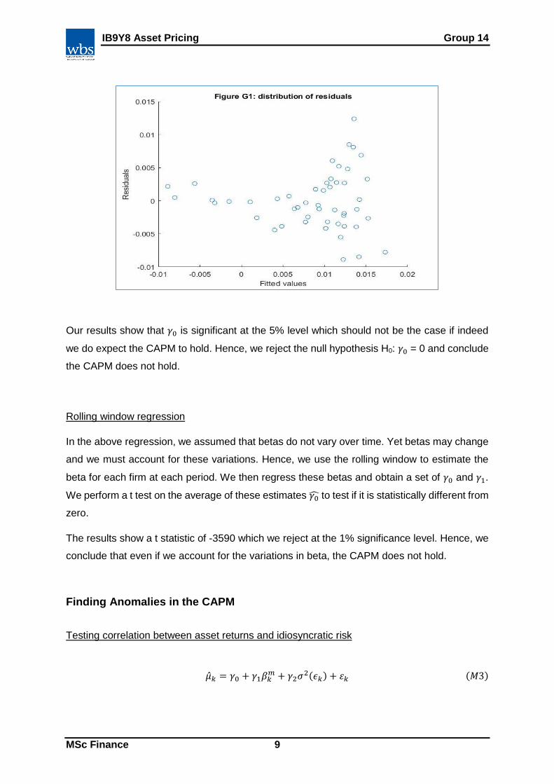
We also test the error terms for normality using the Jarque-Bera (JB) test to ensure that we
can do hypothesis testing on the results. The JB test fails to reject the null hypothesis at the
5% significance level and thus we conclude that the error terms are normally distributed at the
5% significance level. Visually, this can be seen in Figure G1.
IB9Y8 Asset Pricing Group 14
MSc Finance 9
Our results show that 𝛾0 is significant at the 5% level which should not be the case if indeed
we do expect the CAPM to hold. Hence, we reject the null hypothesis H0: 𝛾0 = 0 and conclude
the CAPM does not hold.
Rolling window regression
In the above regression, we assumed that betas do not vary over time. Yet betas may change
and we must account for these variations. Hence, we use the rolling window to estimate the
beta for each firm at each period. We then regress these betas and obtain a set of 𝛾0 and 𝛾1.
We perform a t test on the average of these estimates 𝛾0̂ to test if it is statistically different from
zero.
The results show a t statistic of -3590 which we reject at the 1% significance level. Hence, we
conclude that even if we account for the variations in beta, the CAPM does not hold.
Finding Anomalies in the CAPM
Testing correlation between asset returns and idiosyncratic risk
�̂�𝑘 = 𝛾0 + 𝛾1𝛽𝑘𝑚 + 𝛾2𝜎2(𝜖𝑘) + 𝜀𝑘 (𝑀3)
IB9Y8 Asset Pricing Group 14
MSc Finance 10
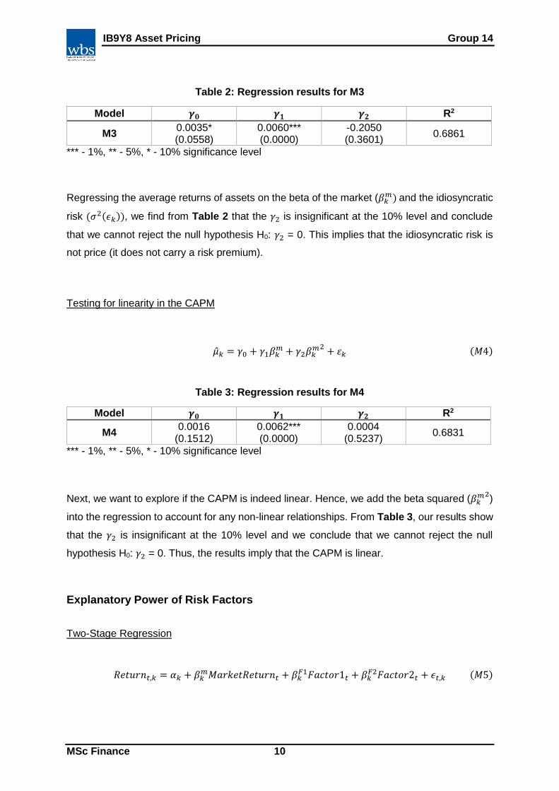
Table 2: Regression results for M3
Model 𝜸𝟎 𝜸𝟏 𝜸𝟐 R2
M3 0.0035* (0.0558)
0.0060*** (0.0000)
-0.2050 (0.3601)
0.6861
*** - 1%, ** - 5%, * - 10% significance level
Regressing the average returns of assets on the beta of the market (𝛽𝑘𝑚) and the idiosyncratic
risk (𝜎2(𝜖𝑘)), we find from Table 2 that the 𝛾2 is insignificant at the 10% level and conclude
that we cannot reject the null hypothesis H0: 𝛾2 = 0. This implies that the idiosyncratic risk is
not price (it does not carry a risk premium).
Testing for linearity in the CAPM
�̂�𝑘 = 𝛾0 + 𝛾1𝛽𝑘𝑚 + 𝛾2𝛽𝑘
𝑚2+ 𝜀𝑘 (𝑀4)
Table 3: Regression results for M4
Model 𝜸𝟎 𝜸𝟏 𝜸𝟐 R2
M4 0.0016
(0.1512) 0.0062*** (0.0000)
0.0004 (0.5237)
0.6831
*** - 1%, ** - 5%, * - 10% significance level
Next, we want to explore if the CAPM is indeed linear. Hence, we add the beta squared (𝛽𝑘𝑚2
)
into the regression to account for any non-linear relationships. From Table 3, our results show
that the 𝛾2 is insignificant at the 10% level and we conclude that we cannot reject the null
hypothesis H0: 𝛾2 = 0. Thus, the results imply that the CAPM is linear.
Explanatory Power of Risk Factors
Two-Stage Regression
𝑅𝑒𝑡𝑢𝑟𝑛𝑡,𝑘 = 𝛼𝑘 + 𝛽𝑘𝑚𝑀𝑎𝑟𝑘𝑒𝑡𝑅𝑒𝑡𝑢𝑟𝑛𝑡 + 𝛽𝑘
𝐹1𝐹𝑎𝑐𝑡𝑜𝑟1𝑡 + 𝛽𝑘𝐹2𝐹𝑎𝑐𝑡𝑜𝑟2𝑡 + 𝜖𝑡,𝑘 (𝑀5)
IB9Y8 Asset Pricing Group 14
MSc Finance 11
We regress the asset return (𝑅𝑒𝑡𝑢𝑟𝑛𝑡,𝑘) on the market return, Factor 1 and Factor 2 to obtain
the beta estimates for each factor. We test if the alphas are jointly equal to zero using the Wald
test, and get a test statistic of 1.6512 with a corresponding p-value of 0.000. Hence, we reject
the null hypothesis at the 1% significance level and conclude that the alphas are jointly not
equal to zero.
�̂�𝑘 = 𝛾0 + 𝛾1𝛽𝑘𝑚 + 𝛾2𝛽𝑘
𝐹1 + 𝛾3𝛽𝑘𝐹2 + 𝜀𝑘 (𝑀6)
Table 4: Regression results for M6
Model 𝜸𝟎 𝜸𝟏 𝜸𝟐 𝜸𝟑 R2
M6 0.0022** (0.0217)
0.0063*** (0.0000)
0.0009** (0.0245)
0.0041 (0.6087)
0.6833
*** - 1%, ** - 5%, * - 10% significance level
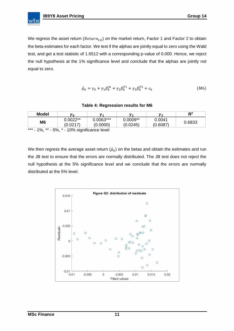
We then regress the average asset return (�̂�𝑘) on the betas and obtain the estimates and run
the JB test to ensure that the errors are normally distributed. The JB test does not reject the
null hypothesis at the 5% significance level and we conclude that the errors are normally
distributed at the 5% level.
IB9Y8 Asset Pricing Group 14
MSc Finance 12
From the regression results in Table 4, we perform hypothesis testing on the individual
significance of the gammas and find that 𝛾2 is significant at the 5% level but, 𝛾3 is not even
significant at the 10% level. Hence, we conclude that Factor 1 does indeed provide additional
explanatory power while Factor 2 does not, i.e. Factor 2 is redundant. Visually, this can be
observed from Figure G2.
Correlation between Pricing Errors and Firm Characteristics
𝑅𝑒𝑡𝑢𝑟𝑛𝑡,𝑘 = 𝛼𝑘 + 𝛽𝑘𝑚𝑀𝑎𝑟𝑘𝑒𝑡𝑅𝑒𝑡𝑢𝑟𝑛𝑡 + 𝛽𝑘
𝐹1𝐹𝑎𝑐𝑡𝑜𝑟1𝑡 + 𝜖𝑡,𝑘 (𝑀7)
Given that we have concluded that Factor 2 is redundant while Factor 1 has explanatory power,
we add Factor 1 into the model (M7) and run the regression to obtain the estimates.
𝛼𝑘 = 𝛽0 + 𝛽1𝐶ℎ𝑎𝑟𝑎𝑐𝑡𝑒𝑟𝑖𝑠𝑡𝑖𝑐1𝑘 + 𝛽2𝐶ℎ𝑎𝑟𝑎𝑐𝑡𝑒𝑟𝑖𝑠𝑡𝑖𝑐2𝑘 + 𝜀𝑘 (𝑀8)
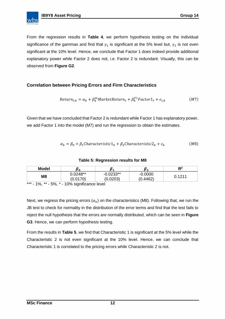
Table 5: Regression results for M8
Model 𝜷𝟎 𝜷𝟏 𝜷𝟐 R2
M8 0.0248** (0.0170)
-0.0233** (0.0203)
-0.0000 (0.4462)
0.1211
*** - 1%, ** - 5%, * - 10% significance level
Next, we regress the pricing errors (𝛼𝑘) on the characteristics (M8). Following that, we run the
JB test to check for normality in the distribution of the error terms and find that the test fails to
reject the null hypothesis that the errors are normally distributed, which can be seen in Figure
G3. Hence, we can perform hypothesis testing.
From the results in Table 5, we find that Characteristic 1 is significant at the 5% level while the
Characteristic 2 is not even significant at the 10% level. Hence, we can conclude that
Characteristic 1 is correlated to the pricing errors while Characteristic 2 is not.
IB9Y8 Asset Pricing Group 14
MSc Finance 13
Building and Testing “Factor-Mimicking Portfolios”
𝑅𝑒𝑡𝑢𝑟𝑛𝑡,𝑘 = 𝛼𝑘 + 𝛽𝑘𝑚𝑀𝑎𝑟𝑘𝑒𝑡𝑅𝑒𝑡𝑢𝑟𝑛𝑡 + 𝛽𝑘
𝐹𝑀𝐹𝑎𝑐𝑡𝑜𝑟𝑀𝑖𝑚𝑖𝑐𝑘𝑖𝑛𝑔𝑡 + 𝜖𝑡,𝑘 (𝑀9)
�̂�𝑘 = 𝛾0 + 𝛾1𝛽𝑘𝑚 + 𝛾2𝛽𝑘
𝐹𝑀 + 𝜀𝑘 (𝑀10)
𝑅𝑒𝑡𝑢𝑟𝑛𝑡,𝑘 = 𝛼𝑘 + 𝛽𝑘𝑚𝑀𝑎𝑟𝑘𝑒𝑡𝑅𝑒𝑡𝑢𝑟𝑛𝑡 + 𝛽𝑘
𝐹1𝐹𝑎𝑐𝑡𝑜𝑟1𝑡 + 𝛽𝑘𝐹𝑀𝐹𝑎𝑐𝑡𝑜𝑟𝑀𝑖𝑚𝑖𝑐𝑘𝑖𝑛𝑔𝑡 + 𝜖𝑡,𝑘 (𝑀11)
�̂�𝑘 = 𝛾0 + 𝛾1𝛽𝑘𝑚 + 𝛾2𝛽𝑘
𝐹1 + 𝛾3𝛽𝑘𝐹𝑀 + 𝜀𝑘 (𝑀12)
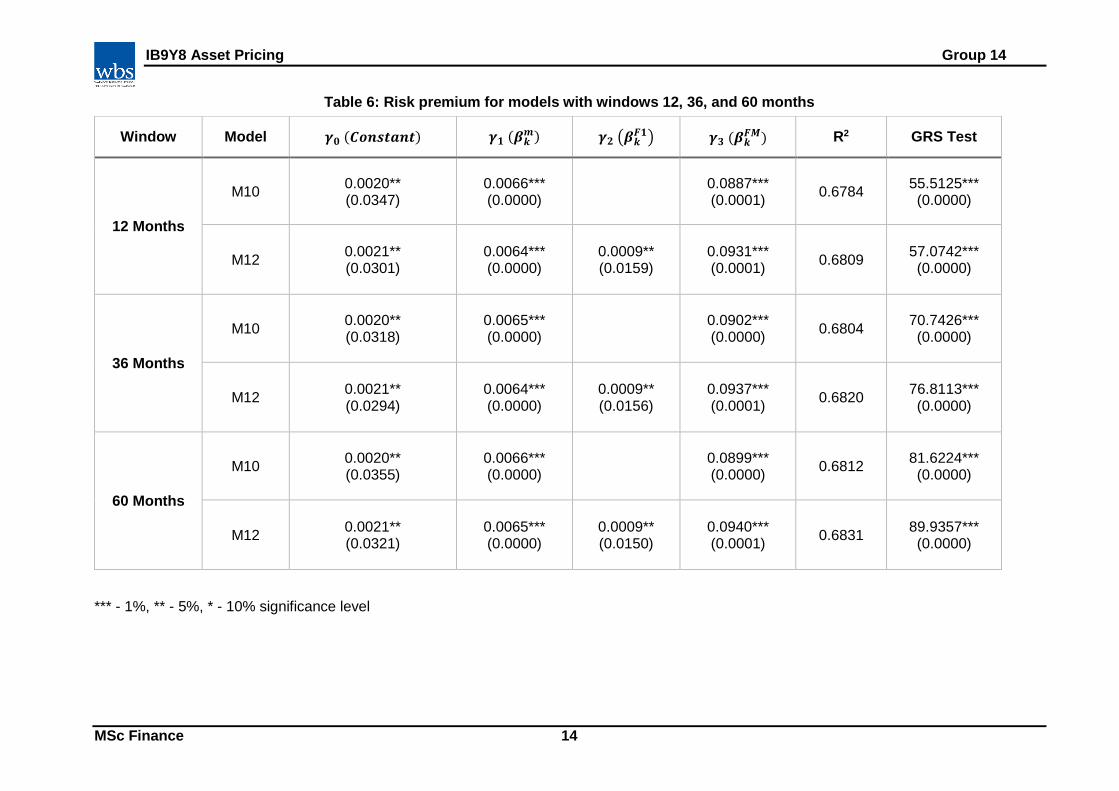
We estimate the betas for both model M9 and M11, using a window of 12, 36, and 60 months
while rebalancing the portfolio every month. Secondly, we regress the average returns on the
beta of the market and these betas to arrive at the models, M10 and M12. From Table 6, our
results show that for all six models we obtained significant results for all 𝛾’s at the 5% level and
1% level. This implies that the model is robust even though the window of estimating betas
change. Furthermore, we also show that the risk factor 1 is significant individually and jointly.
When we examine the R2 of these models, the R2 increases as our window increases from 12
months to 60 months for model M12, which has a value of 0.6809 and 0.6831 respectively.
This suggests that the rolling window estimation is better over 60 months instead of just 12
months.
Lastly, we assume that the error terms follow a normal distribution and conduct the GRS test
for alphas in M9 and M11. The GRS test show that we cannot conclude that the alphas in
these models are jointly equal to zero. Hence, this implies that pricing errors still exist in the
models and we need to add in relevant variables to explain the pricing errors.
IB9Y8 Asset Pricing Group 14
MSc Finance 14
Table 6: Risk premium for models with windows 12, 36, and 60 months
*** - 1%, ** - 5%, * - 10% significance level
Window Model 𝜸𝟎 (𝑪𝒐𝒏𝒔𝒕𝒂𝒏𝒕) 𝜸𝟏 (𝜷𝒌𝒎) 𝜸𝟐 (𝜷𝒌
𝑭𝟏) 𝜸𝟑 (𝜷𝒌𝑭𝑴) R2 GRS Test
12 Months
M10 0.0020** (0.0347)
0.0066*** (0.0000)
0.0887*** (0.0001)
0.6784 55.5125*** (0.0000)
M12 0.0021** (0.0301)
0.0064*** (0.0000)
0.0009** (0.0159)
0.0931*** (0.0001)
0.6809 57.0742*** (0.0000)
36 Months
M10 0.0020** (0.0318)
0.0065*** (0.0000)
0.0902*** (0.0000)
0.6804 70.7426*** (0.0000)
M12 0.0021** (0.0294)
0.0064*** (0.0000)
0.0009** (0.0156)
0.0937*** (0.0001)
0.6820 76.8113*** (0.0000)
60 Months
M10 0.0020** (0.0355)
0.0066*** (0.0000)
0.0899*** (0.0000)
0.6812 81.6224*** (0.0000)
M12 0.0021** (0.0321)
0.0065*** (0.0000)
0.0009** (0.0150)
0.0940*** (0.0001)
0.6831 89.9357*** (0.0000)
IB9Y8 Asset Pricing Group 14
MSc Finance 15
Caveats and Limitations
Earlier, we established two assumptions; error terms are not autocorrelated and no
heteroskedasticity exists. While we do perform the Jarque-Bera test for normality and ensure
that all error terms are normally distributed, i.e. implying that they are not autocorrelated, we
assumed that heteroskedasticity was not present. However, if the assumption was violated,
we would obtain inefficient estimators which may result in the increase in standard errors and
ultimately resulting in the t and F test being invalid.
Secondly, we assume that the stock prices in our data are stationary. However, if these are
indeed nonstationary, this may result in the problem of spurious regression where we
mistakenly fail to reject the factor risk premiums.
Thirdly, a salient limitation in our analysis of the two-stage regression is that the cross-section
regression implicitly assumes that betas do not vary in time. Fama-MacBeth (1973) argues
that by using a rolling window regression we can circumvent this issue. However, the main
drawback of the rolling window regression is that by rebalancing the portfolio we inevitably
overfit the model. This may result in the factor being significant even though it may not actually
be relevant in explaining returns.
Next, when using the rolling window to estimate the factor mimicking portfolio, we rebalance
the portfolio every month and estimate the beta i.e. moving average. However, this may affect
our estimation of betas because we subject our estimation to changes in assets at every period
in our data. Additionally, we choose arbitrary windows (12, 36, and 60 months) to estimate our
betas. While this may account for the variations in beta, it has no economic meaning and is
just taken to represent 1, 3, and 5 years of asset prices.
Moreover, given that the factor-mimicking portfolios are pre-sorted based on their values, it
comes as no surprise that the risk premiums on these factors are significant. This may be
observed by a marginal increase in the R2, even when the factors are added into the model.
With respect to the Wald test, the distribution is assumed to be asymptotically valid. Yet, with
only 50 assets it is arguable that we do not have enough data to make the conjecture about
the validity of the assumptions. Hence, we should use a finite sample test, i.e. GRS test.
Lastly, in conducting the GRS test, we assume that the error terms are normally distributed.
However, this assumption may not hold and the hypothesis test may be invalid if error terms
do not follow a normal distribution.
IB9Y8 Asset Pricing Group 14
MSc Finance 16
Conclusion
In this paper, we have tested the validity of the CAPM using the two-stage regression and the
rolling window regression approach. We use the Wald test to jointly test the null hypothesis
that the pricing errors are equal to zero and show that the CAPM does not hold. Following
Fama-MacBeth (1973), we show that the idiosyncratic risk is not priced and that the CAPM is
linear. We regress the asset returns on the market returns and risk factors and find that only
the risk premia of Factor 1 is significant. Next, we regress pricing errors on the characteristics
and find that only Characteristic 1 is significant in explaining variations in the pricing errors.
We create the factor-mimicking portfolio and obtain the relevant betas and risk premiums.
Finally, we use the GRS test and observe that Factor 1 and the factor-mimicking portfolio do
not fully explain the pricing errors. Hence, we conclude that additional factors are required to
better explain the pricing errors.
IB9Y8 Asset Pricing Group 14
MSc Finance 17
References
Banz, R.W. (1981), “The Relationship between Return and Market Value of Common
Stocks”, Journal of Financial Economics, Vol. 9 No. 1, pp. 3–18.
Basu, S. (1977), “Investment Performance of Common Stocks in Relation to their Price‐
Earnings Ratios: A test of the efficient Market Hypothesis”, Journal of Finance, Vol. 32
No. 3, pp. 663–682.
Carhart, M.M. (1997), “On Persistence in Mutual Fund Performance”, Journal of Finance,
Vol. 52 No. 1, pp. 57–82.
Cochrane, J.H. (2001), Asset Pricing, Princeton, NJ: Princeton University Press.
Fama, E. and MacBeth, J. (1973), “Risk, Return, and Equilibrium: Empirical Tests”, Journal
of Political Economy, Vol. 81 No. 3, p. 607.
Fama, E.F. and French, K.R. (2015), “A Five-Factor Asset Pricing Model”, Journal of
Financial Economics, Vol. 116, pp. 1–22.
Gibbons, M., Ross, S.A. and Shanken, J., “A Test of the Efficiency of a given Portfolio”,
Econometrica: Journal of the Econometric Society, pp. 1121–1152.
Harvey, C.R. (1988), “The Real Term Structure and Consumption Growth”, Journal of
Financial Economics, Vol. 22 No. 2, pp. 305–333.
Hendricks, D., Patel, J. and Zeckhauser, R. (1993), “Hot Hands in Mutual Funds: Short‐Run
Persistence of Relative Performance, 1974–1988”, Journal of Finance, Vol. 48 No. 1, pp.
93–130.
Jarque, C.M. and Bera, A.K. (1980), “Efficient Tests for Normality, Homoscedasticity and
Serial Independence of Regression Residuals”, Economic letters, Vol. 6 No. 3, pp. 225–
259.
Jensen, M.C. (1968), “The Perfomance of Mutual Funds in the Period 1945-1964”, Journal of
Finance, Vol. 23, pp. 389–416.
IB9Y8 Asset Pricing Group 14
MSc Finance 18
Lintner, J. (1965), “The Valuation of Risk Assets and the Selection of Risky Investments in
Stock Portfolios and Capital Budgets”, Review of Economics & Statistics, Vol. 47 No. 1, p.
13.
MacBeth, J.D. (1975), Tests of the two parameter model of capital market equilibrium,
University of Chicago, Graduate School of Business.
Markowitz, H. (1959), “Portfolio Selection: Efficient Diversification of Investments”, Cowles
Foundation Monograph No. 16. New York: John Wiley & Sons, Inc.
Petkova, R. and Zhang, L. (2005), “Is Value riskier than Growth?”, Journal of Financial
Economics, Vol. 78 No. 1, pp. 187–202.
Rosenberg, B., Reid, K. and Lanstein, R. (1985), “Persuasive Evidence of Market
Inefficiency”, The Journal of Portfolio Management, Vol. 11 No. 3, pp. 9–16.
Sharpe, W.F. (1964), “Capital Asset Prices: A Theory of Market Equilibrium under Conditions
of Risk”, Journal of Finance, Vol. 19 No. 3, pp. 425–442.
Stattman, D. (1980), “Book Values and Stock Returns”, The Chicago MBA: A Journal of
Selected Papers, Vol. 4, pp. 25–45.