TESTING CONDITIONAL INDEPENDENCEFOR CONTINUOUS RANDOM VARIABLES

Wicher P. Bergsma†

3-12-2004

Abstract: A common statistical problem is the testing of independence of two (response) variablesconditionally on a third (control) variable. In the first part of this paper, we extend Hoeffding’sconcept of estimability of degree r to testability of degree r, and show that independence is testableof degree two, while conditional independence is not testable of any degree if the control variable iscontinuous. Hence, in a well-defined sense, conditional independence is much harder to test thanindependence. In the second part of the paper, a new method is introduced for the nonparamet-ric testing of conditional independence of continuous responses given an arbitrary, not necessarilycontinuous, control variable. The method allows the automatic conversion of any test of indepen-dence to a test of conditional independence. Hence, robust tests and tests with power againstbroad ranges of alternatives can be used, which are favorable properties not shared by the mostcommonly used test, namely the one based on the partial correlation coefficient. The method isbased on a new concept, the partial copula, which is an average of the conditional copulas. Thefeasibility of the approach is demonstrated by an example with medical data.

Keywords: tests of conditional independence, estimability and testability of degree r, partial copula,partial correlationAMS Subject Classification: Primary 62H15; secondary 62E99

†EURANDOM, PO Box 513, 5600 MB Eindhoven

i

Contents

1 Introduction 1

2 Degree of testability of (conditional) independence 22.1 Testability of degree r . . . . . . . . . . . . . . . . . . . . . . 22.2 Testability of (conditional) independence without assumptions 32.3 Testability of (conditional) independence with assumptions . 6

3 The partial copula 83.1 Definition and basic properties . . . . . . . . . . . . . . . . . 83.2 Kernel estimation . . . . . . . . . . . . . . . . . . . . . . . . . 10

4 Example 11

5 Summary 16

References 18

1 Introduction

For a given triple of random variables (X, Y, Z) we consider the problem ofthe nonparametric testing of the hypothesis of conditional independence of Yand Z controlling for X based on n independent and identically distributed(iid) data points (X1, Y1, Z1), . . . , (Xn, Yn, Zn). Following Dawid (1979), thishypothesis is denoted as Y⊥⊥Z|X.

For the testing of unconditional independence between two random vari-ables a wide array of tests is available, with the best known ones basedon the Pearson correlation, Spearman’s rank correlation, or Kendall’s tau.Tests of unconditional independence which have asymptotic power againstall alternatives were proposed by Hoeffding (1948b) and Schweizer and Wolff(1981).

In contrast, for the (nonparametric) testing of conditional independencethere appears to be only one commonly used method, namely the test basedon the partial correlation coefficient. With g(x) = E(Y |X = x) and h(x) =E(Z|X = x), it is defined as

ρ(Y, Z|X) =ρ(g(X), h(X))− ρ(X, g(X))ρ(X,h(X))√

(1− ρ(X, g(X))2)(1− ρ(X, h(X))2)(1)

In fact, ρ(Y, Z|X) equals the correlation between the errors in the regressionsy = g(x)+ε1 and z = h(x)+ε2. Evaluation of the test requires the estimationof the regression curves g and h. An alternative method, which does notappear to be used often, was proposed by Goodman (1959) and is basedon a partial version of Kendall’s tau, using the number of local concordantand discordant pairs of observations. This test was further discussed inGoodman and Grunfeld (1961) and Gripenberg (1992). Some well-knownother tests are based on the linear partial correlation coefficient, which is (1)with g and h replaced by the identity function, or on Kendall’s partial tau(Kendall, 1942). However, it is well-known that these coefficients are notnecessarily zero under conditional independence unless certain restrictiveconditions are met, severely limiting their applicability (Korn, 1984).

Note that the above remark regarding the limited number of tests ofconditional independence applies only if the control variable X is continuous.If X is categorical, with sufficiently many observations per category, it is notdifficult to devise a test of conditional independence: for each category, atest of independence can be done, and these tests can be combined in variousways. If all three variables are categorical, log-linear techniques can be used(cf. Lauritzen, 1996).

1

Summarizing, a flexible array of tests of conditional independence with acontinuous control variable appears to be unavailable in the literature, andthis paper aims to fill that gap. First, in Section 2, the theoretical difficultieswith the testing of conditional independence are investigated and it is shownthat with a continuous control variable, the problem is in a well-defined senseharder than the testing of unconditional independence. Then in Section 3 anew testing methodology is presented, using which any test of unconditionalindependence can be used to construct a test of conditional independence.Evaluation of the test requires the estimation of certain conditional marginalquantiles of Y given X and of Z given X. Although this is about the sameamount of work as the estimation of the regression curves in (1), it leads toa much more flexible class of test statistics. In Section 4, the feasibility ofthe approach is demonstrated by an example with medical data.

2 Degree of testability of (conditional) indepen-dence

In this section we first introduce the concept of testability of degree r, whichis an extension of Hoeffding’s concept of estimability of degree r, and thenapply it to the hypotheses of independence and conditional independence.It is shown that independence is testable of degree 2, while conditionalindependence is not testable of degree r for any r. Finally, it is shown thatif the (conditional) marginal distributions are known, both hypotheses aretestable of degree 1.

2.1 Testability of degree r

Hoeffding (1948a) defined the concept of estimability of degree r, which werestate as follows:

Definition 1 For a set of probability measures P, a parameter θ : P → Ris called estimable of degree r if r is the smallest number for which there isa function h : Rr → R such that, for all P ∈ P,

θ(P ) = Eh(X1, . . . , Xr)

if the Xi are iid according to P .

Related to Hoeffding’s concept, we introduce the concept of testability ofdegree r:

2

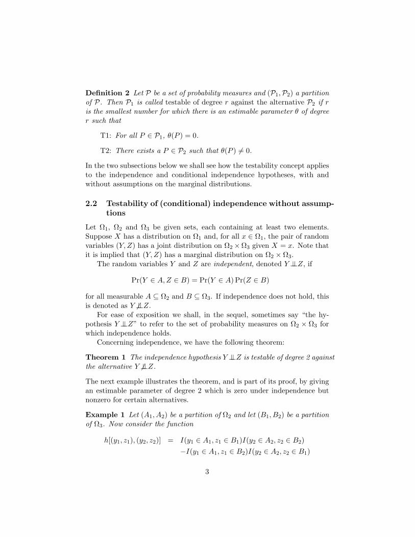
Definition 2 Let P be a set of probability measures and (P1,P2) a partitionof P. Then P1 is called testable of degree r against the alternative P2 if ris the smallest number for which there is an estimable parameter θ of degreer such that

T1: For all P ∈ P1, θ(P ) = 0.

T2: There exists a P ∈ P2 such that θ(P ) 6= 0.

In the two subsections below we shall see how the testability concept appliesto the independence and conditional independence hypotheses, with andwithout assumptions on the marginal distributions.

2.2 Testability of (conditional) independence without assump-tions

Let Ω1, Ω2 and Ω3 be given sets, each containing at least two elements.Suppose X has a distribution on Ω1 and, for all x ∈ Ω1, the pair of randomvariables (Y, Z) has a joint distribution on Ω2×Ω3 given X = x. Note thatit is implied that (Y, Z) has a marginal distribution on Ω2 × Ω3.

The random variables Y and Z are independent, denoted Y⊥⊥Z, if

Pr(Y ∈ A,Z ∈ B) = Pr(Y ∈ A) Pr(Z ∈ B)

for all measurable A ⊆ Ω2 and B ⊆ Ω3. If independence does not hold, thisis denoted as Y 6⊥⊥Z.

For ease of exposition we shall, in the sequel, sometimes say “the hy-pothesis Y⊥⊥Z” to refer to the set of probability measures on Ω2 × Ω3 forwhich independence holds.

Concerning independence, we have the following theorem:

Theorem 1 The independence hypothesis Y⊥⊥Z is testable of degree 2 againstthe alternative Y 6⊥⊥Z.

The next example illustrates the theorem, and is part of its proof, by givingan estimable parameter of degree 2 which is zero under independence butnonzero for certain alternatives.

Example 1 Let (A1, A2) be a partition of Ω2 and let (B1, B2) be a partitionof Ω3. Now consider the function

h[(y1, z1), (y2, z2)] = I(y1 ∈ A1, z1 ∈ B1)I(y2 ∈ A2, z2 ∈ B2)−I(y1 ∈ A1, z1 ∈ B2)I(y2 ∈ A2, z2 ∈ B1)

3

where I is the indicator function, equalling 1 if its argument is true and 0otherwise. Then if Y⊥⊥Z and if (Y1, Z1) and (Y2, Z2) are iid and distributedas (Y, Z), it is straightforward to verify that

Eh[(Y1, Z1), (Y2, Z2)] = 0

Furthermore, if (Y ′, Z ′) are such that

Pr(Y ′ ∈ A1, Z′ ∈ B1) = Pr(Y ′ ∈ A2, Z

′ ∈ B2) =12

then for iid (Y ′i , Z ′i) distributed as (Y ′, Z ′),

Eh[(Y ′1 , Z

′1), (Y

′2 , Z

′2)] =

146= 0

Hence, the estimable parameter θ of degree 2 based on the function h satisfiesthe conditions T1 and T2.

Proof of Theorem 1: Let P be the set of probability measures onΩ2 × Ω3. Further, let P1 ⊆ P be the set of probability measures satisfyingthe independence hypothesis and let P2 be its complement in P. Supposeθ is an estimable parameter of degree 1 which satisfies condition T1 andwhich is based on a certain function h. Let P ∈ P be degenerate satisfyingP (a, b) = 1 for certain a ∈ Ω2 and b ∈ Ω3. Then it immediately follows thatP ∈ P1. Therefore, by condition T1, θ(P ) = 0, implying h(a, b) = 0. Sincea and b were arbitrary, h is zero on its domain and hence θ(P ) = 0 for allP ∈ P. Therefore condition T2 does not hold, and so, since θ was chosenarbitrarily, the independence hypothesis is not testable of degree 1. That itis testable of degree 2 follows from Example 1. 2

The random variables Y and Z are conditionally independent given X,denoted Y⊥⊥Z|X, if

Pr(Y ∈ A,Z ∈ B|X = x) = Pr(Y ∈ A|X = x) Pr(Z ∈ B|X = x)

for all x ∈ Ω1 and measurable A ⊆ Ω2 and B ⊆ Ω3. If conditional indepen-dence does not hold, this is denoted as Y 6⊥⊥Z|X.

The random variable X is called continuous if P (X = x) = 0 for allx in the domain of X. Theorem 2 shows that, with a continuous controlvariable, testing conditional independence is, in a well-defined sense, muchharder than testing independence.

4

Theorem 2 Under the restriction that X is continuous, there is no r suchthat the conditional independence hypothesis Y⊥⊥Z|X is testable of degree ragainst the alternative Y 6⊥⊥Z|X.

Proof of Theorem 2: Let P be the set of probability measures on Ω =Ω1 × Ω2 × Ω3 with continuous marginal distribution on Ω1, i.e.,

P (x × Ω2 × Ω3) = 0

for all P ∈ P and x ∈ Ω1. It is assumed that for all x ∈ Ω1 the conditionalmeasures on x × Ω2 × Ω3 are also defined. Let P1 be the set of proba-bility measures in P satisfying conditional independence and let P2 be itscomplement in P.

Suppose, for certain r, θ is an estimable parameter of degree r whichsatisfies condition T1 and which is based on a certain function h. For arbi-trary (x1, y1, z1), . . . , (xr, yr, zr) in Ω with xi 6= xj if i 6= j let P ∈ P be thedegenerate distribution satisfying

P [(x1, y1, z1), . . . , (xr, yr, zr)] = 1

Then it immediately follows that P ∈ P1. Therefore, by condition T1,θ(P ) = 0, implying

h[(x1, y1, z1), . . . , (xr, yr, zr)] = 0

Since the (xi, yi, zi) were arbitrary, h is zero on its domain except possiblyon a set with measure zero (where xi = xj for some i 6= j). Hence θ(P ) = 0for all P ∈ P, so condition T2 does not hold for θ. Therefore, since θ waschosen arbitrarily, P1 is not testable of degree r against P2. Since r wasarbitrary, the theorem is proven. 2

An intuition for Theorem 2 is as follows. If X is continuous, then an iidsample (Xi, Yi, Zi) has, with probability one, at most one observed (Y, Z)pair for any value of X. Theorem 1 indicates that at least two pairs wouldbe needed in order to have any ‘information’ on the conditional dependencefor the corresponding value of X.

Summarizing, Theorems 1 and 2 indicate a fundamental difference be-tween the testing of independence and of conditional independence with acontinuous control variable.

5

2.3 Testability of (conditional) independence with assump-tions

In this section we show that given assumptions about the (conditional)marginal distributions, (conditional) independence hypotheses are testableof degree 1. This result is especially useful for the conditional independencehypothesis with a continuous control variable, since, by Theorem 2, it is nottestable of any degree. However, it also indicates a fundamental difficulty:assumptions must be made in order to be able to obtain a test. For thetesting of independence this is, of course, not necessary.

A distribution is called degenerate if all its probability mass is concen-trated on one point. The next theorem shows the effect of incorporatingassumptions about the marginal distributions of Y and Z on the testabilityof Y⊥⊥Z.

Theorem 3 Suppose Y and Z have given non-degenerate marginal distri-butions. Then the hypothesis Y⊥⊥Z is testable of degree 1 against the alter-native Y 6⊥⊥Z.

To prove the theorem, it suffices to give an example of an estimable param-eter of degree 1 satisfying the conditions T1 and T2, as is done next.

Example 2 If Y and Z have given non-degenerate marginal distributions,there is an A ⊂ Ω2 such that

0 < Pr(Y ∈ A) < 1

and a B ⊂ Ω3 such that

0 < Pr(Z ∈ B) < 1

Using the shorthand p = Pr(Y ∈ A) and q = Pr(Z ∈ B), consider thefunction

h(y, z) = I(y ∈ A, z ∈ B)− pq

Then

θ = Eh(Y, Z) = Pr(Y ∈ A,Z ∈ B)− pq

is zero if Y⊥⊥Z and nonzero if, for example,

Pr(Y ∈ A,Z ∈ B) = min(p, q)

Hence, the estimable parameter θ of degree 1 based on the function h satisfiesthe conditions T1 and T2.

6

Theorem 2 suggests the hypothesis Y⊥⊥Z|X is ‘untestable.’ However,as indicated by Theorem 4, appropriate assumptions about the conditionaldistributions of Y and Z given X render the hypothesis testable.

Theorem 4 Suppose for all x ∈ Ω1, both the marginal distributions of Yand Z given X = x are known and non-degenerate. Then the hypothesisY⊥⊥Z|X is testable of degree 1 against the alternative Y 6⊥⊥Z|X .

The following example illustrates and proves the theorem for arbitrary Ω1, Ω2

and Ω3.

Example 3 Suppose, for all x, Y and Z have given non-degenerate marginaldistributions given X = x. Then for any x there is an A(x) ⊂ Ω2 such that

0 < Pr[Y ∈ A(x)|X = x] < 1

and a B(x) ⊂ Ω3 such that

0 < Pr[Z ∈ B(x)|X = x] < 1

Using the shorthand p(x) = Pr[Y ∈ A(x)|X = x] and q(x) = Pr[Z ∈B(x)|X = x], consider the function

h(x, y, z) = I[y ∈ A(x), z ∈ B(x)]− p(x)q(x)

Then, for all x,

Eh(x, Y, Z) = Pr[Y ∈ A(x), Z ∈ B(x)]− p(x)q(x)

is zero if Y⊥⊥Z|X and nonzero if, for example,

Pr(Y ∈ A(x), Z ∈ B(x)|X = x) = min(p(x), q(x)) (2)

for all x. Hence,

θ = Eh(X,Y, Z) =∫

Eh(x, Y, Z)dP1(x)

is zero if Y⊥⊥Z|X and nonzero if (2) holds. Therefore, the estimable pa-rameter θ of degree 1 based on the function h satisfies the conditions T1 andT2.

7

3 The partial copula

In this section an automatic conversion procedure is presented by whichany test of unconditional independence can be used to obtain a test of con-ditional independence. For this purpose, the partial copula is introduced,which has the salient feature that independence holds for the partial cop-ula if conditional independence holds for the responses given the control.A kernel estimation method for the partial copula is introduced, which in-volves estimating conditional marginal distributions of the responses giventhe control.

3.1 Definition and basic properties

Suppose Y and Z are real-valued random variables with conditional distri-bution functions

F2|1(y|x) = Pr(Y ≤ y|X = x)F3|1(z|x) = Pr(Z ≤ z|X = x)

A basic property of

U = F2|1(Y |X)

and

V = F3|1(Z|X)

is given in the following lemma.

Lemma 1 Suppose, for all x, F2|1(y|x) is continuous in y and F3|1(z|x) iscontinuous in z. Then U and V have uniform marginal distributions.

Proof of Lemma 1: By continuity of F2|1(y|x) in y, and with F1 themarginal distribution function of X,

Pr(U ≤ u) = Pr(F2|1(Y |X) ≤ u)

=∫

Pr(F2|1(Y |x) ≤ u)dF1(x)

=∫

udF1(x)= u

i.e., the marginal distribution of U is uniform. The uniformity of the distri-bution of V is shown analogously. 2

8

The importance of the introduction of U and V lies in the followingtheorem.

Theorem 5 Suppose, for all x, F2|1(y|x) is continuous in y and F3|1(z|x)is continuous in z. Then Y⊥⊥Z|X implies U⊥⊥V .

Proof of Theorem 5: By Lemma 1, U and V are uniformly distributed.Hence if Y⊥⊥Z|X the joint distribution function of U and V simplifies asfollows:

Pr(U ≤ u, V ≤ v) = Pr(F2|1(Y |X) ≤ u, F3|1(Z|X) ≤ v)

=∫

Pr(F2|1(Y |x) ≤ u, F3|1(Z|X) ≤ v)dF1(x)

=∫

Pr(F2|1(Y |x) ≤ u) Pr(F3|1(Z|X) ≤ v)dF1(x)

=∫

uvdF1(x)= uv

= Pr(U ≤ u) Pr(V ≤ v)

This completes the proof. 2

For continuous random variables Y and Z with marginal distributionfunctions F and G, the copula of their joint distribution is defined as thejoint distribution of F (Y ) and G(Z). The copula is said to contain the grade(or rank) association between Y and Z (for an overview, see Nelsen, 1998).For example, Kendall’s tau and Spearman’s rho are functions of the copula.The following definition gives an extension of the copula concept.

Definition 3 The joint distribution of U and V is called the partial copulaof the distribution of Y and Z given X.

Note that the conditional copula, denoted C23|1, is given as

C23|1(u, v|x) = Pr(F2|1(Y |X = x) ≤ u, F3|1(Z|X = x) ≤ v)

and that the partial copula, say G23, is the average conditional copula, givenby the formula

G23(u, v) = EC23|1(u, v|X) =∫

C23|1(u, v|x)dF1(x) (3)

Theorem 5 implies that a test of (marginal) independence of U and V isa test of conditional independence of Y and Z given X. It should be noted

9

that since U⊥⊥V does not imply Y⊥⊥Z|X, a test of the hypothesis U⊥⊥Vcannot have power against all alternatives of the hypothesis Y⊥⊥Z|X. Inparticular, this is so for alternatives with interaction, that is, where theassociation between Y and Z depends on the value of X. We should expectmost power against alternatives with a constant conditional copula, i.e.,alternatives for which the joint distribution of (F2|1(Y |x), F3|1(Z|x)) doesnot depend on x. A test of independence of U and V can be done by anystandard procedure.

An example of the derivation of U and V in a parametric setting is givennext.

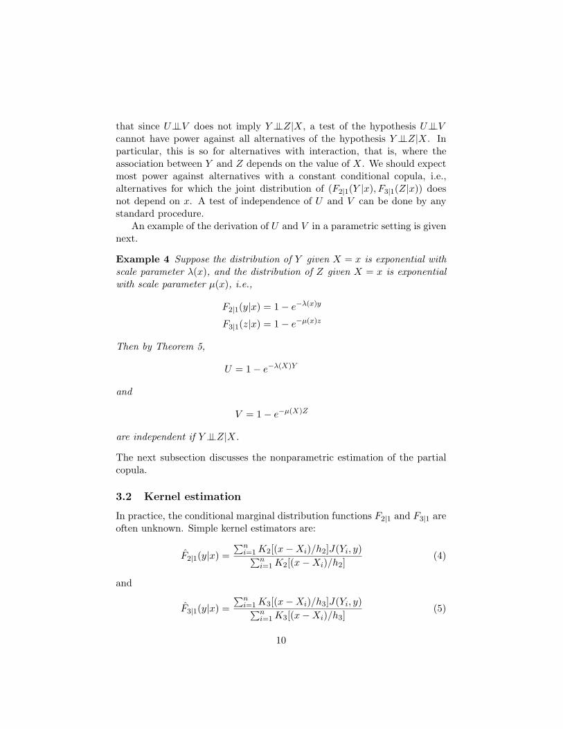
Example 4 Suppose the distribution of Y given X = x is exponential withscale parameter λ(x), and the distribution of Z given X = x is exponentialwith scale parameter µ(x), i.e.,

F2|1(y|x) = 1− e−λ(x)y

F3|1(z|x) = 1− e−µ(x)z

Then by Theorem 5,

U = 1− e−λ(X)Y

and

V = 1− e−µ(X)Z

are independent if Y⊥⊥Z|X.

The next subsection discusses the nonparametric estimation of the partialcopula.

3.2 Kernel estimation

In practice, the conditional marginal distribution functions F2|1 and F3|1 areoften unknown. Simple kernel estimators are:

F2|1(y|x) =∑n

i=1 K2[(x−Xi)/h2]J(Yi, y)∑ni=1 K2[(x−Xi)/h2]

(4)

and

F3|1(y|x) =∑n

i=1 K3[(x−Xi)/h3]J(Yi, y)∑ni=1 K3[(x−Xi)/h3]

(5)

10

where h > 0 is the bandwidth, usually dependent on n, and K the kernelfunction, which can be a density symmetric around zero and

J(x, y) =

0 x < y12

x = y1 x > y

A suitable choice for K is often the standard normal distribution.Consider the new observations (Ui, Vi), given as

Ui = F2|1(Yi|Xi) (6)

Vi = F3|1(Zi|Xi) (7)

Now a test of independence of U and V based on the (Ui, Vi) is a test ofconditional independence of Y and Z given X based on the (Xi, Yi, Zi).An example is given in the next section. A heuristic argument that the(Ui, Vi) may be treated as iid observations for sufficiently large n is as follows.Standard results can be used to show that, if h2n and h3n go to zero at asufficiently fast rate, and under suitable (light) regularity conditions, both

(√n(F2|1(y|x)− F2|1(y|x)),

√n(F2|1(y′|x′)− F2|1(y′|x′)

)

and(√

n(F3|1(z|x)− F3|1(z|x)),√

n(F3|1(z′|x′)− F3|1(z′|x′))

have an asymptotic bivariate normal distribution with correlation equal tozero for all (x, y, z) 6= (x′, y′, z′).

4 Example

Table 1 shows data on 35 consecutive patients under treatment for heartfailure with the drug digoxin. The data are from Halkin, Sheiner, Peck,and Melmon (1975). Of medical interest is the hypothesis that digoxinclearance is independent of urine flow controlling for creatinine clearance,i.e., Y⊥⊥Z|X. Edwards (2000) based his analyses on the partial correlationcoefficient (1) assuming linear regression functions g and h. Then (1) reducesto

ρY Z|X =ρY Z − ρXY ρXZ√

(1− ρ2XY )(1− ρ2

XZ)

11

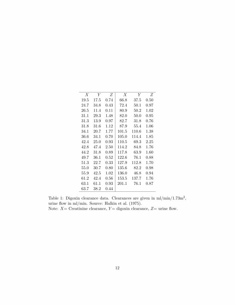
X Y Z X Y Z19.5 17.5 0.74 66.8 37.5 0.5024.7 34.8 0.43 72.4 50.1 0.9726.5 11.4 0.11 80.9 50.2 1.0231.1 29.3 1.48 82.0 50.0 0.9531.3 13.9 0.97 82.7 31.8 0.7631.8 31.6 1.12 87.9 55.4 1.0634.1 20.7 1.77 101.5 110.6 1.3836.6 34.1 0.70 105.0 114.4 1.8542.4 25.0 0.93 110.5 69.3 2.2542.8 47.4 2.50 114.2 84.8 1.7644.2 31.8 0.89 117.8 63.9 1.6049.7 36.1 0.52 122.6 76.1 0.8851.3 22.7 0.33 127.9 112.8 1.7055.0 30.7 0.80 135.6 82.2 0.9855.9 42.5 1.02 136.0 46.8 0.9461.2 42.4 0.56 153.5 137.7 1.7663.1 61.1 0.93 201.1 76.1 0.8763.7 38.2 0.44

Table 1: Digoxin clearance data. Clearances are given in ml/min/1.73m2,urine flow in ml/min. Source: Halkin et al. (1975).Note: X= Creatinine clearance, Y = digoxin clearance, Z= urine flow.

12

20 40 60 80 100 120 140Y

50

100

150

200

X

20 40 60 80 100 120 140Y

0.5

1

1.5

2

2.5

Z

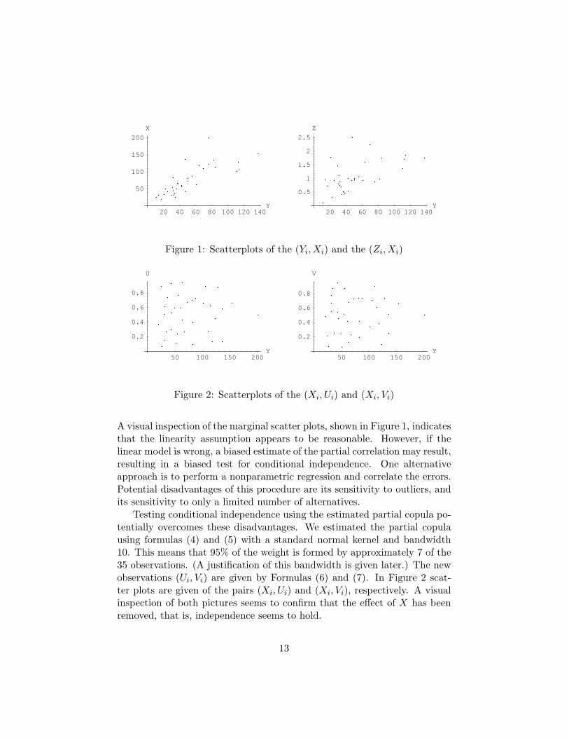
Figure 1: Scatterplots of the (Yi, Xi) and the (Zi, Xi)

50 100 150 200Y

0.2

0.4

0.6

0.8

U

50 100 150 200Y

0.2

0.4

0.6

0.8

V

Figure 2: Scatterplots of the (Xi, Ui) and (Xi, Vi)

A visual inspection of the marginal scatter plots, shown in Figure 1, indicatesthat the linearity assumption appears to be reasonable. However, if thelinear model is wrong, a biased estimate of the partial correlation may result,resulting in a biased test for conditional independence. One alternativeapproach is to perform a nonparametric regression and correlate the errors.Potential disadvantages of this procedure are its sensitivity to outliers, andits sensitivity to only a limited number of alternatives.

Testing conditional independence using the estimated partial copula po-tentially overcomes these disadvantages. We estimated the partial copulausing formulas (4) and (5) with a standard normal kernel and bandwidth10. This means that 95% of the weight is formed by approximately 7 of the35 observations. (A justification of this bandwidth is given later.) The newobservations (Ui, Vi) are given by Formulas (6) and (7). In Figure 2 scat-ter plots are given of the pairs (Xi, Ui) and (Xi, Vi), respectively. A visualinspection of both pictures seems to confirm that the effect of X has beenremoved, that is, independence seems to hold.

13

0.2 0.4 0.6 0.8U

0.2

0.4

0.6

0.8

V

-1.5 -1 -0.5 0 0.5 1 1.5F-1HUL-1.5

-1

-0.5

0

0.5

1

1.5

F-1HVL

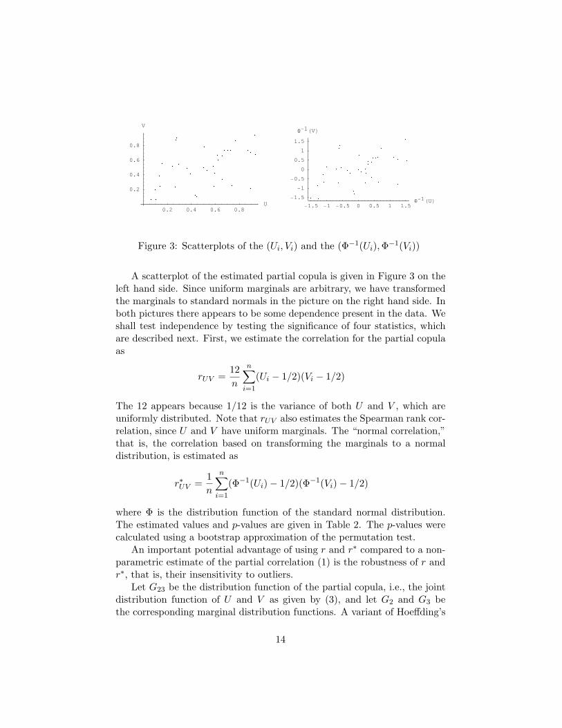
Figure 3: Scatterplots of the (Ui, Vi) and the (Φ−1(Ui), Φ−1(Vi))

A scatterplot of the estimated partial copula is given in Figure 3 on theleft hand side. Since uniform marginals are arbitrary, we have transformedthe marginals to standard normals in the picture on the right hand side. Inboth pictures there appears to be some dependence present in the data. Weshall test independence by testing the significance of four statistics, whichare described next. First, we estimate the correlation for the partial copulaas

rUV =12n

n∑

i=1

(Ui − 1/2)(Vi − 1/2)

The 12 appears because 1/12 is the variance of both U and V , which areuniformly distributed. Note that rUV also estimates the Spearman rank cor-relation, since U and V have uniform marginals. The “normal correlation,”that is, the correlation based on transforming the marginals to a normaldistribution, is estimated as

r∗UV =1n

n∑

i=1

(Φ−1(Ui)− 1/2)(Φ−1(Vi)− 1/2)

where Φ is the distribution function of the standard normal distribution.The estimated values and p-values are given in Table 2. The p-values werecalculated using a bootstrap approximation of the permutation test.

An important potential advantage of using r and r∗ compared to a non-parametric estimate of the partial correlation (1) is the robustness of r andr∗, that is, their insensitivity to outliers.

Let G23 be the distribution function of the partial copula, i.e., the jointdistribution function of U and V as given by (3), and let G2 and G3 bethe corresponding marginal distribution functions. A variant of Hoeffding’s

14

coefficient (Hoeffding, 1948b) measuring the dependence between U and Vis

HUV =∫

[G23(y, z)−G2(y)G3(z)]2 dydz

To obtain Hoeffding’s coefficient, dydz has to be replaced by dG23(y, z).Both Hoeffding’s coefficient and HUV share the property that they are non-negative and equal to zero if and only if U and V are independent. A con-venient way to estimate HUV is by using a formula developed by (Bergsma,2004), given as

HUV = E(|U ′

1 − U ′2| − |U ′

1 − U ′3|

) (|V ′1 − V ′

2 | − |V ′2 − V ′

4 |)

where (U ′1, V

′1), . . . , (U

′4, V

′4) are iid and distributed as (U, V ). Hence, the

unbiased U-statistic estimator of HUV is given as

HUV =

(n4

)−1 ∑(|Ui − Uj | − |Ui − Uk|) (|Vi − Vj | − |Vj − Vl|)

where the sum is taken over all i, j, k, l unequal. Like the correlation, HUV

is also evaluated for both the partial copula with uniform and with normalmarginals, the latter denoted as H∗

UV . In Table 2, estimated values of Hand H∗ are given, together with p-values for the hypothesis that they arezero. The p-values were calculated by a bootstrap approximation of thepermutation test.

The reason we have chosen HUV rather than Hoeffding’s coefficient is toavoid unnecessary discretization. Hoeffding’s test is based on the ranks ofthe observations (like Kendall’s tau and Spearman’s rho). One of the reasonsto use a rank test is to deal with outliers and to control the marginals bymaking them uniform. In the present case, the (theoretical) distributionof U and V is already uniform, thereby making a further ranking of the(Ui, Vi) unnecessary, and this would only cause unnecessary discretizationof the data. For the same reason, we have not considered Kendall’s tau andSpearman’s rho.

An important potential advantage of using H and H∗ to test for inde-pendence between U and V is that they yield asymptotic power against allalternatives with dependence. This is something that cannot be achievedwith the partial correlation coefficient (1).

A justification of the choice of bandwidth has not been given. As thebandwidth approaches zero, the (Ui, Vi) converge to ( 1

2, 1

2). Thus, all of the

estimators above converge to zero. The bandwidth should be chosen large

15

Coefficient Estimated value p-valueρUV .372 .0062ρ∗UV .314 .0031HUV .656 .0032H∗

UV .651 .0077

Table 2: Estimated values of some coefficients and their bootstrap p-values.Based on the data of Table 1

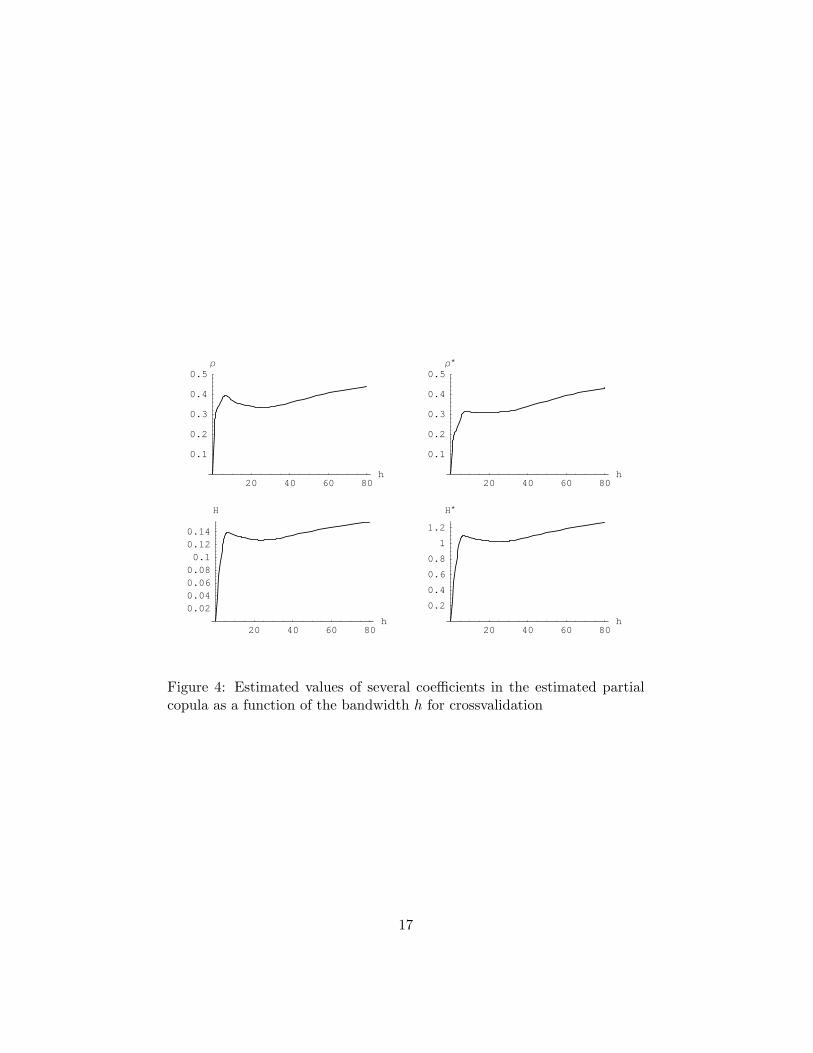
enough that at least one point in the neighborhood has sufficient weight. Forcrossvalidation purposes, the estimated parameters are plotted as a functionof the bandwidth h in Figure 4. For all coefficients, the method appears tobreak down when the bandwidth h < 6, and the value h = 10 appears to bereasonable. Note that a crossvalidation should always be performed.

5 Summary

In Section 2, the concept of testability of degree r, which is related toHoeffding’s concept of estimability of degree r, was defined. It was shownthat independence is testable of degree 2 while, for a continuous controlvariable, conditional independence is not testable of any degree. Then itwas shown that, if the conditional marginal distributions of responses givencontrol are known, the conditional independence hypothesis is testable ofdegree 1. Hence, the testing of conditional independence is more difficultthan the testing of unconditional independence, in the sense that the formerrequires assessment of the conditional marginal distributions.

In Section 3, the results of Section 2 were used to derive a practicaltesting procedure, which makes it possible to convert an arbitrary test ofindependence to a test of conditional independence. This was done by in-troducing the partial copula which is a function of the original trivariatedistribution. Like the copula, the partial copula is a bivariate distributionwith uniform marginals. Additionally, it has the property of satisfying in-dependence if conditional independence holds for the original distribution.Hence, any test of independence applied to the partial copula is a test of con-ditional independence applied to the original distribution. Estimation of thepartial copula requires the conditional marginal distributions of responsesgiven control which are usually unknown in practice, and a kernel estimatorwas proposed. Thus, a wide range of tests is obtained whose evaluation is

16

20 40 60 80h

0.020.040.060.080.10.120.14

H

20 40 60 80h

0.2

0.4

0.6

0.8

1

1.2

H*

20 40 60 80h

0.1

0.2

0.3

0.4

0.5Ρ

20 40 60 80h

0.1

0.2

0.3

0.4

0.5Ρ*

Figure 4: Estimated values of several coefficients in the estimated partialcopula as a function of the bandwidth h for crossvalidation

17

no more difficult than nonparametric estimation of the partial correlationcoefficient.

The method was illustrated by an example in Section 4. Two tests relatedto the rank correlation were described. These directly compete with thepartial correlation, but have the advantage of robustness. Two other testsrelated to a test of Hoeffding (1948b) were also described, and these havethe advantage of asymptotic power against a broad range of alternatives.

References

Bergsma, W. P. (2004). Absolute correlation. Unpublished manuscript.

Dawid, A. P. (1979). Conditional independence in statistical theory (withdiscussion). J. Roy. Statist. Soc. Ser. B, 41, 1-31.

Edwards, D. (2000). Introduction to graphical modelling. New York:Springer verlag.

Goodman, L. A. (1959). Partial tests for partial tau. Biometrika, 46,425-432.

Goodman, L. A., & Grunfeld, Y. (1961). Some nonparametric tests forcomovements between time series. Journal of the American StatisticalAssociation, 56, 11-26.

Gripenberg, G. (1992). Partial rank correlations. Journal of the AmericanStatistical Association, 87, 546-551.

Halkin, H., Sheiner, L. B., Peck, C. C., & Melmon, K. L. (1975). Determi-nants of the renal clearance of digoxin. Clin. Pharmocol. Theor., 17,385-394.

Hoeffding, W. (1948a). A class of statistics with asymptotically normaldistribution. Annals of Mathematical Statistics, 19, 293-325.

Hoeffding, W. (1948b). A non-parametric test of independence. Annals ofMathematical Statistics, 19, 546-557.

Kendall, M. G. (1942). Partial rank correlation. Biometrika, 32, 277-283.

Korn, E. L. (1984). The ranges of limiting values of some partial correlationsunder conditional independence. The American Statistician, 38, 61-62.

18

Lauritzen, S. L. (1996). Graphical models. Oxford: Clarendon Press.

Nelsen, R. B. (1998). An introduction to copulas. New York: Springer.

Schweizer, B., & Wolff, E. F. (1981). On nonparametric measures of depen-dence for random variables. Annals of Statistics, 9, 879-885.

19