Testing Divergent Natural Selection onMorphology of Crossbills (Loxia sp.)

Tianhong Gong

Degree project in biology, Master of science (2 years), 2009Examensarbete i biologi 45 hp till masterexamen, 2009Biology Education Centre and Department of Animal Ecology, Uppsala UniversitySupervisors: Dr. Pim Edelaar and Prof. Mats Björklund

1

Index

Summary .......................................................................................................................................... 2

Section 1 Comparisons of neutral genetic differentiation at marker loci and quantitative traits

Introduction ..................................................................................................................................... 4

Materials and Methods ................................................................................................................... 5

Study species and areas ......................................................................................................... 5

Microsatellite analysis .......................................................................................................... 7

Morphometric variation analysis .......................................................................................... 7

FST and QST comparisons ....................................................................................................... 9

Results ............................................................................................................................................ 11

Check for population substructure ...................................................................................... 11

Repeatability Check ............................................................................................................. 12

Comparing QST in bill depth and FST across 11 split crossbill populations ........................ 12

Testing the effect of resource similarity on QST values across 11 populations ................... 14

Comparing QST in bill depth and FST across 4 lumped crossbill populations ..................... 14

Comparing QST in mandible angles and FST across 3 lumped crossbill populations .......... 16

Discussion....................................................................................................................................... 18

Section 2 Do scaly leg mites cause selection on crossbill morphology?

Introduction ................................................................................................................................... 22

Materials and Methods ................................................................................................................. 23

Data collection .................................................................................................................... 23

Statistical analyses .............................................................................................................. 23

Results ............................................................................................................................................ 26

Discussion....................................................................................................................................... 30

Conclusion ..................................................................................................................................... 32

Acknowledgements........................................................................................................................ 33

References ...................................................................................................................................... 34

2

Summary

A most fascinating feature of life is its diversity. The origin of biodiversity is an

important field for evolutionary studies. Particularly, the study of adaptive radiation

will help us to understand the origin of biodiversity. Crossbills (Loxia spp.) are

songbirds characterized by the mandibles crossing at the tips, and are highly

specialized to their food resources – seeds in conifer cones. Based on their extreme

resource specialization, bill size and shape of crossbills are thought have a great

influence on fitness through their effect on food intake. In the first section of this

report, we try to test whether diversification of morphology among crossbills is best

explained by natural selection or by random genetic drift. This is done by comparing

neutral genetic with quantitative morphological differentiation, estimated respectively

as FST and QST among crossbill populations. The basic prediction is that divergent

natural selection is implied when FST < QST, while convergent natural selection is

suggested when FST > QST. When FST = QST, the hypothesis of neutrality (no selection

on the quantitative trait) cannot be excluded. Comparisons of FST and QST across

populations revealed that the degree of differentiation in the quantitative traits of bill

depth and bill tip angles exceeds that of neutral marker loci (microsatellites) in most

cases, suggesting that divergent selection potentially caused by use of food resource

was detected. On the other hand, other selective forces that are unrelated to resource

use may also cause population differentiation. For example, one study showed that

ectoparasitic scaly-leg mites can differentially infect crossbills, so that mite-induced

mortality caused directional selection favoring smaller bill depth. Thus, in the second

section, we followed up on this study and investigated the relationship between mite

infection and morphological traits as well as other potential factors (sex, age, catching

month, to which ‘vocal type’/population the crossbills belonged). Infections with

mites were significantly more common in crossbills with longer wings and tarsi.

Additionally, vocal types differed significantly in infection rate, and thus selection by

mites could have caused the observed morphological differentiation of vocal types.

Overall, we found support for the hypothesis that resource use can drive the adaptive

radiation of crossbill morphology, but other selective forces such as scaly-leg mites

can confound evolutionary patterns.

3

Section 1

Comparisons of neutral genetic differentiation at

marker loci and quantitative traits

4

Introduction

Divergent selection on quantitative traits is considered the ultimate cause of

phenotypic differentiation in adaptive radiation. It may occur in spatially separated

populations inhabiting different environments, or among sympatric morphs or closely

related species exploiting different resources. Comparatively, convergent selection can

lead to the same phenotype in different populations. Although natural selection may

be primarily responsible for patterns of phenotypic variation in natural population,

random genetic drift is also a potential force driving population differentiation in

quantitative traits (Lande 1976). The comparison of genetic differentiation at

microsatellite marker loci and at loci coding for quantitative traits was used to

distinguish the cause of geographical variation, as measured by FST and QST

respectively. The basic prediction of divergent selection is that, if certain

morphological traits play a key role contributing to adaptation, independent

populations adapted to different environments should diverge in morphology, whereas

those adapted to similar environments should tend to be similar. If QST > FST,

divergent selection on the quantitative trait is implied; if QST < FST, the effect of

convergent selection pressure is revealed; if QST = FST, neutral expectation that the

quantitative trait is not exposed to selection cannot be excluded (Merilae & Crnokrak

2001).

Crossbills (Loxia spp.) are songbirds characterized by the mandibles crossing at the

tips and are highly specialized for foraging on the seeds of conifer cones (Benkman

1993). Crossbills use their crossed mandibles to bite between overlapping cone scales

and then laterally abduct the lower mandible to the side to which it crosses, leading to

the separation of cone scales and the exposition of seeds (Benkman 1996). The size

and shape of bills are considered have a great influence on their foraging efficiency

(Benkman 1993, Benkman & Miller 1996) and thus the targets of selection since

feeding rates can affect fitness (Benkman 2003). Furthermore, bill depth is the

morphological trait most closely related to foraging ability in crossbills (Benkman

1993, Benkman 2003) and the ratio of bill depth divided by bill length is suggested

highly related to shape rather than size of bills (Borrás et al. 2008).

In this section, we mainly aim to distinguish whether a diversification of morphology

among crossbills is caused by natural selection or random genetic drift. We focus on

the study of bills, the morphological character under relatively important selection

pressure (Benkman 2003). To involve both the size and shape of bills in, bill depth

and the sum of upper and lower mandible angles were chosen as our target phenotypic

traits, assuming the latter one equivalent to the index bill depth/bill length. QST was

estimated on these two morphological traits, while FST estimate was based on

microsatellite studies. Pair-wise comparisons of FST and QST estimates were

performed firstly across 11 crossbill populations grouped by the catching sites. Then

with the aim to get more reliable estimates, we lumped these 11 populations into 4

groups with larger sample sizes according to the use of conifer resources, because

populations of crossbills are suggested to be recognized by key food resources rather

than by geographical localities (Benkman 1993, Edelaar et al. 2003).

5

Materials and Methods

Study species and areas

Blood samples of common crossbill (Loxia curvirostra) were obtained by Daniel

Alonso and Pim Edelaar in Spain from April of 2001 to November of 2007. The

summary of populations used in our study is given in Table 1.1, with information

about their catching sites, food resources, observers and sample sizes. Samples were

collected from the continental areas of Spain including Navarra, Alicante, Málaga, La

Rioja, Teruel, Guadalajara and Catalunya, as well as Mallorca, the largest island of

Spain (Fig. 1.1). Additionally, in this study three pine species were considered:

Aleppo pine Pinus halepensis, Scotch pine P. sylvestris and mountain pine P. uncinata.

Fig. 1.1. Distribution of the sampling localities for common crossbills: 1) Sierra de Maigmó (Alicante)

2) Calvia (Mallorca) 3) Montes de Málaga (Málaga) 4) Sierra de Jabalambre (Valencia) 5) Lakuaga

Navarra) 6) Lando, Leire (Navarra) 7) Tendilla (Guadalajara) 8) Chiquicos, Ejulve (Teruel) 9) Sierra

Gúdar, Valdelinares (Teruel) 10) Sierra Turza (La Rioja) 11) Pyrenees (Catalunya)The map is made by

Google Earth.

6

Table 1.1. Information on the crossbill samples in the study, including population names, state provinces, catching locations, pine species used as resource, observers and

sample sizes used for the calculations of FST and QST. All samples were collected in Spain.

Pop. Province Location Coordinate Conifer Observer N(FST) N(QST)

H_Mai Alicante Sierra de Maigmó 38º32' N 00º35' W P. halepensis Alonso and Edelaar 35 60

H_Maj Mallorca Calvia 39º34' N 02º30' E P. halepensis Alonso and Edelaar 35 32

H_Mal Málaga Montes de Málaga 36º49' N 04º21' W P. halepensis Alonso 30 59

H_SdJ Valencia Sierra de Jabalambre 39º53' N 00º58' W P. halepensis Alonso 30 30

H_Ten Guadalajara Tendilla 40º33' N 02º58' W P. halepensis Alonso 33 29

H_Ter Teruel Chiquicos, Ejulve 40º46' N 00º33' W P. halepensis Alonso 29 29

S_Lak Navarra Lakuaga 42º52' N 00º59' W P. sylvestris Alonso 21 25

S_Lan Navarra Lando, Leire 42º40' N 01º08' W P. sylvestris Alonso 13 24

S_LaR La Rioja Sierra Turza 42º21' N 03º15' W P. sylvestris Alonso 30 30

S_Ter Teruel Sierra Gúdar, Valdelinares 40º23' N 00º38' W P. sylvestris Alonso 33 40

U_Cat Catalunya ski-base 42º10' N 01º32' E P. uncinata Edelaar 27 25

Total

316 383

7

Microsatellite analysis

DNA was extracted from 352 blood samples of crossbills in total, using FTA-paper

and classic Chelex (5%) method respectively for 279 birds trapped by Alonso and 73

by Edelaar, following the manufacturer’s protocol. After extraction, DNA

concentration was measured with a spectrophotometer. To identify different

microsatellite loci, the polymerase chain reaction (PCR) amplification was carried out

using four different primer-pairs (Ase42, Lox6, Lox3 and Lox7) in a final 10μl

volume with 1.0μl 10×PCR buffer (with MgCl2), 0.1μl TAQ polymerase, 6.3μl

ddH20, 0.8μl dNTPs, and 0.4μl of each primer. The amplification was performed

under standard conditions as follows: one step of initial denaturation lasted for 2 min

at 94°C, followed by 35 cycles of 30s 94°C as the denature step, 30s at X°C

annealing primer with single strand DNA template, and 30s 72°C as the primer

extension step. Here X=60, 54, 61 and 55 respectively for Ase42, Lox6, Lox3 and

Lox7.

Fluorescent labeling of the forward PCR primers was used to detect amplification

products on an ABI Prism®

377 automated sequencer (Applied Biosystems). The

DNA fragment sizing was carried out using GeneScan®

and allele designations were

made in Genotyper® (Applied Biosystems). The fixation index FST both for all pairs of

samples and a single measure for all samples were obtained from the software

GenePop. Samples from a few populations were composed of birds caught in different

years or different locations and population subdivision for microsatellite loci with

high mutation rates relative to allozymes may cause a deviation of FST estimation

(Hedrick 1999), so we checked firstly for any significant population substructure to

eliminate the underestimation of population subdivision.

Morphometric variation analysis

To study the morphometric variation of crossbills, measurements on many traits were

taken from living crossbills as mentioned in the first section and some additional

measurements were made from the digital photographs taken by Edelaar. Five

biometric variables were measured for the crossbill specimens from Barcelona

museums: M1 - background scales (from start to end of 5 squares), M2 - upper

mandible depth (from start of feathering to tip), M3 -lower mandible depth (from start

of feathering to narrowest part of lower mandible), A4 and A5 - upper and lower bill

angles (base-tip-base). Only last four measurements were taken for the images of

living birds in the field without scale-background. The TpsDig software was used for

digitizing landmarks and outlines for geometric morphometric analyses and the linear

distances and angles shown in Fig. 1.2. TpsUtil was used to randomly scramble the

8

order of specimens in a tps file to minimize bias in digitizing landmark locations,

which helps to eliminate the effect of systematic error in a time series.

Based on the extraordinary specialization on food resource for the crossbills, we

predicted that diversity of pine species is considered as natural selection for crossbills

with influence on the fitness. Therefore, we chose the depth and angle of bills as

target traits for the following reasons. In many previous studies bill depth has been

shown as the trait most closely related to foraging ability in crossbills (Benkman 1993;

Benkman 2003), and it varies among crossbills inhabited in different pine areas

(Borrás et al. 2008). The angles of upper and lower mandibles are considered an

indicator of bill shape (James 2003), similar as the index bill depth/bill length which

also provides very significant differences between birds of different habitats (Borrás

et al. 2008). We used the sum of the two angles as the variable taking account that the

blunter state occurs in both of the upper and lower mandibles and thus the sum should

show the greatest effect as expected.

Fig. 1.2. Five measurements on morphological traits taken from image, respectively as upper mandible

bill depth (M2), lower mandible bill depth (M3), upper bill angle (A4) and lower bill angle (A5).

A4

A5

M2

M3

9

Firstly, to confirm the reliability of data, repeatability (r) was calculated. Repeatability

is used to test the precision on measurements taken by a single person or instrument

on the same item under the same conditions. The denotation of repeatability

coefficient is r = s2

A

s2+s2A , where the among-groups variance component (s2

A) and the

within group variance component (s2) are estimated by mean squares of the variables

and errors in the analysis of variance: s2 = MSw and s2A =

MS A−MS w

n0 where n0 is a

coefficient to estimate the sample size per group. Here n0 is calculated as follows,

n0 =1

a−1[ ni

ai=1 −

n i2a

i=1

n iai=1

], a is the number of groups and ni is the sample size in

the i th group (Lessells and Boag 1987). In our study, five measurements were taken

twice by the same person with a time interval of four months on 34 crossbills from

Barcelona museums.

The calculation of QST is defined as s2

s2+2s2A for diploids (Latta 1998). One-way

ANOVA was first performed on the bill depth trait to remove the effect of following

variables: population, sex, age, year and observer. All measures were ln-transformed

and standardized to a mean of zero and a standard deviation of one. Then

MeanSquares of the variables and errors were obtained to estimate variances among

and within populations from the result of ANOVA analysis on the residuals of ln-

transformed bill depth in regard to the effect of populations.

FST and QST comparisons

Comparisons between putatively neutral genetic differentiation and quantitative

genetic variation were used to test for natural selection, by measuring the index values

of FST and QST following a FST-QST scatterplot of pair wise populations grouping by

resource similarity. However, this comparison method is challenging because the

assertion that neutral FST should equal QST for neutral traits under neutral evolution is

not completely true due to the variable values of neutral FST and QST (Whitlock 2008).

Some factors such as direct selection, indirect effects of selection, sampling errors and

genetic drift can induce FST estimates to vary among loci. Also, QST is very difficult to

measure precisely and estimates can be biased for unreliable traits that are predicted

to be under spatially varying selection or as a result of biased estimation of the genetic

variation within and among populations (Whitlock 2008). Therefore, we increased the

sample sizes by lumping the eleven small populations into four populations according

to resource habitats as Table 1.2 shows, improving the precision of QST and making

FST less heterogeneous. The population from Mallorca was split as a specific one due

to its isolated geographical environment.

10

All the comparisons mentioned above on the variable of bill depth were performed

both across the 11 split and 4 lumped populations. However, due to the lack of related

measurements in the sylvestris population, morphological differentiation on the angles

was distinguished only in the following lumped populations: halepensis,

halepensis_M, and uncinata. For the uncinata population, the measurements were

taken on specimens of Barcelona museums for the absence of living samples.

Additionally, the distributions of QST and FST are well approximated by the Lewontin-

Krarkauer prediction, suggesting a new method to compare QST to the distribution

rather than to the mean of FST values for a single trait. Specifically, we made a more

reliable inference to determine if QST was significantly smaller or larger than a given

FST from the ratio (ndemes − 1) QST /FST following a chi-squared distribution

with (ndemes − 1) degrees of freedom.

Table 1.2. Corresponding information of four lumped populations with eleven split small populations.

Lumped Population Split populations

halepensis_M H_Maj

halepensis H_Mai, H_Mal, H_SdJ, H_Ten, H_Ter

sylvestris S_Lak, S_Lan, S_LaR, S_Ter

uncinata U_Cat

11

Results

Check for population substructure

We checked for substructure within populations according to different years or

catching sites (Table 1.3). The result in FST analysis across all loci shows a few

indications of substructure in some groups of crossbills, especially the case for the

crossbills from Lakuaga measured in different years shows a relatively large FST with

highly significant p-value. However, taking into account for the furthering studies of

QST, we still considered them one population and lumped all samples within

populations.

Table 1.3. Check for substructure in the following populations: H_Maj, H_Ter, S_Lan and S_Lak, by

lumping or splitting small populations according to different factors such as catching place or year.

Negative values of FST were adjusted to 0.00. For the population names, A and C denote two different

sites on the Mallorca Isaland; the numbers denote the years (e.g. 7=2007); P denote that Pim Edelaar

collected the samples while Alonso did that without P in the name.

POP Grouping POPA NA POPB NB FST p-value

H_Maj

Four small

pop.

H_Maj_A1 7 H_Maj_C1 9 0.01 0.02

H_Maj_A1 7 H_Maj_C2 16 0.02 0.04

H_Maj_A1 7 H_Maj_C7_P 3 0.02 0.05

H_Maj_C1 9 H_Maj_C2 16 0.00 0.14

H_Maj_C1 9 H_Maj_C7 3 0.01 0.15

H_Maj_C2 16 H_Maj_C7_P 3 0.02 0.11

Place H_Maj_A 7 H_Maj_(C1+C2

+C7_P) 28 0.02 0.01

Year

H_Maj_(A1+C1) 16 H_Maj_C2 16 0.002 0.06

H_Maj_(A1+C1) 16 H_Maj_C7_P 3 0.008 0.02

H_Maj_C2 16 H_Maj_C7_P 3 0.00 0.10

Person H_Maj_(A1+C1+C2) 32 H_Maj_C7_P 3 0.00 0.02

H_Ter Year H_Ter6 5 H_Ter7 24 0.00 0.004

S_Lan Year S_Lan1 5 S_Lan4 8 0.00 0.13

S_Lak Year S_Lak1 13 S_Lak4 8 0.05 <0.00001

12

Repeatability Check

Repeatability is reliable according to the results from ANOVA in separate individuals

given as Table 1.4, in which number of groups (a) is 34, and sample size (ni) is 2 in

each group.

Table 1.4. Analysis of variance (ANOVA) for the calculation of repeatability on measures in different

individuals (crossbills from Barcelona and field). The definitions of measurements follow the

description in the beginning part of morphological variation analysis.

Measurement F ratio (d.f.=33, 34) s2 s2A r P-value

M1 58.2 2.08 59.5 0.966 <0.001

M2 26.3 16.7 210 0.927 <0.001

M3 30.8 11.4 170 0.937 <0.001

A4 6.27 1.35 3.57 0.725 <0.001

A5 12.9 1.33 7.91 0.856 <0.001

Comparing QST in bill depth and FST across 11 split crossbill populations

For eleven populations, calculation of FST and QST with p-values for bill depth is

shown in Table 1.5. Since variance components cannot be negative, some small

negative values were adjusted upwards to zero. A comparison of FST and QST (Fig. 1.3)

indicates that QST exceeds FST in most cases. However, QST nearly equals or is less

than FST in a few comparisons, specifically, H_Maj & H_Mai, H_Maj & S_LaR,

H_Maj & H_SdJ, H_Maj & H_Ter, H_SdJ & S_LaR and S_Lak & U_Cat.

Table 1.5. Synopsis of pairwise FST and QST values in 11 populations. The column ‘resource’ indicates

whether the 2 populations are using the same or different conifers as resource.

POP A POP B Resource No s2 s2A Adj. QST P(QST) Adj. FST P(FST)

H_Mai H_Maj Same 41 0.0001 <0.0001 0.01 0.19 0.04 <0.01

H_Mai H_Mal Same 58 0.0001 <0.0001 0.11 <0.01 0.01 <0.01

H_Mai H_SdJ Same 40 0.0002 0.0000 0.00 0.57 0.00 0.05

H_Mai H_Ten Same 39 0.0002 0.0002 0.33 <0.01 0.00 0.03

H_Mai H_Ter Same 39 0.0002 0.0000 0.00 0.40 0.00 0.01

H_Mai S_Lak Different 34 0.0001 0.0002 0.39 <0.01 0.00 <0.01

H_Mai S_Lan Different 33 0.0001 0.0001 0.32 <0.01 0.02 <0.01

H_Mai S_LaR Different 38 0.0002 0.0000 0.00 0.99 0.01 <0.01

H_Mai S_Ter Different 48 0.0002 0.0002 0.37 <0.01 0.01 <0.01

H_Mai U_Cat Different 35 0.0001 0.0001 0.30 <0.01 0.00 <0.01

H_Maj H_Mal Same 40 0.0001 0.0001 0.21 <0.01 0.04 <0.01

H_Maj H_SdJ Same 30 0.0002 <0.0001 0.02 0.15 0.03 <0.01

H_Maj H_Ten Same 30 0.0002 0.0001 0.21 <0.01 0.04 <0.01

13

H_Maj H_Ter Same 30 0.0002 0.0000 0.03 0.10 0.03 <0.01

H_Maj S_Lak Different 27 0.0002 0.0003 0.44 <0.01 0.04 <0.01

H_Maj S_Lan Different 26 0.0002 0.0002 0.39 <0.01 0.03 <0.01

H_Maj S_LaR Different 29 0.0002 <0.0001 0.00 0.34 0.03 <0.01

H_Maj S_Ter Different 35 0.0002 0.0002 0.26 <0.01 0.02 <0.01

H_Maj U_Cat Different 28 0.0002 0.0002 0.37 <0.01 0.03 <0.01

H_Mal H_SdJ Same 39 0.0001 <0.0001 0.05 0.02 0.00 <0.01

H_Mal H_Ten Same 38 0.0002 0.0004 0.53 <0.01 0.00 <0.01

H_Mal H_Ter Same 38 0.0001 <0.0001 0.04 0.05 0.01 <0.01

H_Mal S_Lak Different 34 0.0001 0.0001 0.23 <0.01 0.00 <0.01

H_Mal S_Lan Different 33 0.0001 <0.0001 0.15 <0.01 0.01 <0.01

H_Mal S_LaR Different 38 0.0001 <0.0001 0.08 0.01 0.02 <0.01

H_Mal S_Ter Different 47 0.0002 0.0004 0.56 <0.01 0.01 <0.01

H_Mal U_Cat Different 35 0.0001 <0.0001 0.13 <0.01 0.01 <0.01

H_SdJ H_Ten Same 29 0.0003 0.0002 0.29 <0.01 0.00 0.38

H_SdJ H_Ter Same 29 0.0002 0.0000 0.00 0.83 0.00 0.64

H_SdJ S_Lak Different 27 0.0002 0.0001 0.28 <0.01 0.00 0.21

H_SdJ S_Lan Different 26 0.0002 0.0001 0.22 <0.01 0.00 0.14

H_SdJ S_LaR Different 29 0.0002 0.0000 0.00 0.69 0.00 0.03

H_SdJ S_Ter Different 34 0.0003 0.0003 0.34 <0.01 0.00 0.23

H_SdJ U_Cat Different 27 0.0002 0.0001 0.20 <0.01 0.00 0.01

H_Ten H_Ter Same 29 0.0003 0.0002 0.31 <0.01 0.00 0.06

H_Ten S_Lak Different 26 0.0003 0.0008 0.60 <0.01 0.00 0.16

H_Ten S_Lan Different 26 0.0002 0.0007 0.57 <0.01 0.01 0.04

H_Ten S_LaR Different 28 0.0003 0.0002 0.25 <0.01 0.01 <0.01

H_Ten S_Ter Different 34 0.0003 0.0000 0.00 0.63 0.00 0.12

H_Ten U_Cat Different 27 0.0003 0.0007 0.56 <0.01 0.00 0.05

H_Ter S_Lak Different 26 0.0002 0.0001 0.26 <0.01 0.00 0.05

H_Ter S_Lan Different 26 0.0002 0.0001 0.20 <0.01 0.00 0.27

H_Ter S_LaR Different 28 0.0002 0.0000 0.00 0.55 0.00 <0.01

H_Ter S_Ter Different 34 0.0003 0.0003 0.36 <0.01 0.00 <0.01

H_Ter U_Cat Different 27 0.0002 0.0001 0.18 <0.01 0.00 <0.01

S_Lak S_Lan Same 23 0.0001 0.0000 0.00 0.46 0.00 0.03

S_Lak S_LaR Same 26 0.0002 0.0002 0.31 <0.01 0.01 <0.01

S_Lak S_Ter Same 30 0.0002 0.0008 0.64 <0.01 0.00 <0.01

S_Lak U_Cat Different 24 0.0002 0.0000 0.00 0.42 0.00 0.01

S_Lan S_LaR Same 25 0.0002 0.0001 0.25 <0.01 0.00 0.68

S_Lan S_Ter Same 29 0.0002 0.0007 0.61 <0.01 0.00 0.04

S_Lan U_Cat Different 24 0.0002 0.0000 0.00 0.93 0.00 0.01

S_LaR S_Ter Same 33 0.0003 0.0002 0.30 <0.01 0.00 <0.01

S_LaR U_Cat Different 26 0.0002 0.0001 0.23 <0.01 0.00 <0.01

S_Ter U_Cat Different 31 0.0002 0.0007 0.60 <0.01 0.00 0.06

(Continued Table 1.5.)

14

Fig. 1.3. Scatterplot of FST-QST pairwise comparisons in 11 populations pairs using as listed in Table

2.5. Black discs denote the same resources; circles denote use of different food resource.

Testing the effect of resource similarity on QST values across 11 populations

A Kruskal-Wallis test (non-parametric ANOVA) was used to check if there was an

effect of food resource similarity on QST in 11 split populations. The Chi-square value

is approximately 0.0055 (d.f.=1), p = 0.94, so we cannot reject the null hypothesis that

there is no effect of resource similarity on QST.

Comparing QST in bill depth and FST across 4 lumped crossbill populations

For four lumped populations, descriptive statistics of the variable bill depth is shown

in Table 1.6. It seems that the bill depth of crossbills in the halepensis_M population

is smaller than the average level while the variable of crossbills in the uncinata

population is larger. The calculation of FST and QST with p-values and a scatterplot of

pairwise FST-QST values are separately shown in Table 1.7 and in Fig. 1.4. Chi-

squared tests (d.f.= ndemes-1) were made for the null hypothesis that there was no

0.0 0.2 0.4 0.6 0.8

0.0

0.2

0.4

0.6

0.8

Adjusted FST

Ad

just

ed Q

ST

15

larger morphological differentiation in bill depth than in neutral markers. The results

indicate that the difference between FST and QST in the comparisons involving the

uncinata population is more significant compared to comparisons among other

populations. The results across the four populations show that the divergence between

QST and FST estimates is significantly from zero within populations, and that QST is

significantly larger than FST.

Table 1.6. LS mean values and standard errors of bill length for 4 lumped populations (halepensis,

halepensis_M, sylvestris and uncinata) of crossbills, followed with sample size. F3,371= 7.52 (P<0.0001).

Population LS Mean SE N

halepensis 10.53 0.030 204

halepensis_M 10.45 0.077 31

sylvestris 10.54 0.040 115

uncinata 10.94 0.086 25

Table 1.7. Summary statistics of adjusted values of FST and QST on bill depth for 4 lumped populations.

The estimated ratio (ndemes − 1) QST /FST follows a chi-squared distribution with (ndemes-1) degrees of

freedom. (ndemes-1) is 1 for pairwise analysis and is 3 for the analysis across the four lumped

populations.

POP A POP B No QST P (QST) FST P(FST) (ndemes-1)QST/FST P(ratio)

halepensis_M halepensis 54 0.003 0.24 0.03 <.0001 0.10 0.75

halepensis_M sylvestris 49 0.00* 0.45 0.03 <.0001 0.00 >0.999

halepensis_M uncinata 28 0.37 0.00 0.03 <.0001 11.1 <0.005

halepensis sylvestris 147 0.00* 0.91 0.002 <.0001 0.00 1.00

halepensis uncinata 45 0.21 0.00 0.003 0.009 82.2 <0.0001

sylvestris uncinata 41 0.12 0.001 0.00* 0.34 Infinite <0.0001

Across 4 populations 75 0.04 < 0.001 0.01 <.0001 11.0 <0.0001

*Adjusted from negative values to zero

16

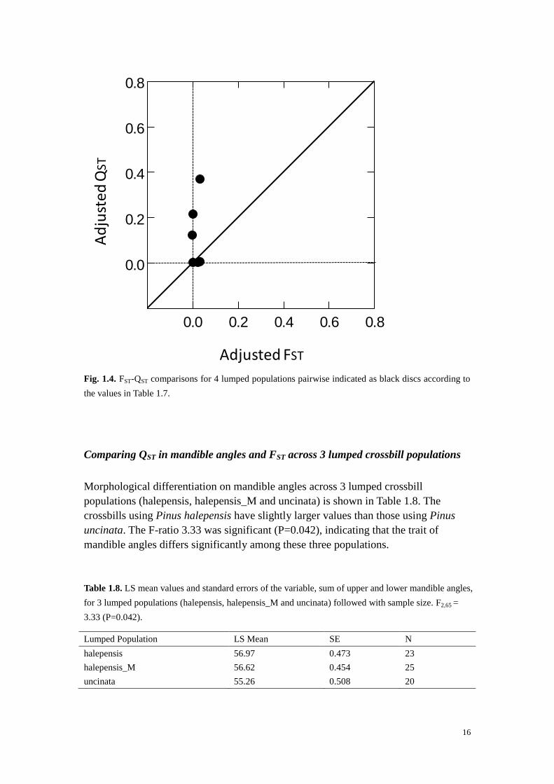
Fig. 1.4. FST-QST comparisons for 4 lumped populations pairwise indicated as black discs according to

the values in Table 1.7.

Comparing QST in mandible angles and FST across 3 lumped crossbill populations

Morphological differentiation on mandible angles across 3 lumped crossbill

populations (halepensis, halepensis_M and uncinata) is shown in Table 1.8. The

crossbills using Pinus halepensis have slightly larger values than those using Pinus

uncinata. The F-ratio 3.33 was significant (P=0.042), indicating that the trait of

mandible angles differs significantly among these three populations.

Table 1.8. LS mean values and standard errors of the variable, sum of upper and lower mandible angles,

for 3 lumped populations (halepensis, halepensis_M and uncinata) followed with sample size. F2,65 =

3.33 (P=0.042).

Lumped Population LS Mean SE N

halepensis 56.97 0.473 23

halepensis_M 56.62 0.454 25

uncinata 55.26 0.508 20

0.0 0.2 0.4 0.6 0.8

0.0

0.2

0.4

0.6

0.8A

dju

sted

QST

Adjusted FST

17

Similar as the FST-QST analysis on the variable of bill depth, the generalized linear

model (GLM) method was performed on the sum of upper and lower mandible angles

in these three lumped populations. The results in Table 1.9 and Fig. 1.5 show that the

difference between genetic divergence and quantitative divergence is significant in the

uncinata population while the difference between FST and QST in the Mallorca

population seems not significant consistent with the former analysis on bill depth.

Across the three lumped populations, there is no significant difference between FST

and QST on the trait of mandible angles.

Table 1.9. Adjusted values of FST and QST obtained from Genepop and GLM analysis respectively, with

p-value. The estimated ratio (ndemes − 1) QST /FST follows a chi-squared distribution with (ndemes-1)

degrees of freedom. ndemes-1 is 1 for pairwise analysis and 2 for the analysis across the three lumped

populations.

POPA POPB N0 QST P(QST) FST P(FST) (ndemes-1)QST/FST P(ratio)

halepensis_M halepensis 24 0.00 0.55 0.03 0.00 0.00 1.00

halepensis_M uncinata 22 0.05 0.07 0.03 0.00 1.61 0.21

halepensis uncinata 21 0.10 0.02 0.003 0.03 39.0 <.0001

Across 3 populations 45 0.03 0.04 0.02 0.04 2.29 0.11

Fig. 1.5. Fst-Qst pairwise comparisons for three lumped populations. The dependent variable is the sum

of upper and lower mandible angles by ln-transformation.

0.00 0.05 0.10 0.15

0.00

0.05

0.10

0.15

Adjusted FST

Ad

juste

d Q

ST

18

Discussion

To ensure FST a biased estimate of genetic differentiation in neutral marker loci, we

checked the population subdivision firstly and detected the substructure in the

Mallorca population, which is actually difficult for us to understand. We viewed the

output of Genepop and found that the hyper variation was mainly caused by highly

significant genetic differentiation within the Mallorca population on one locus, Lox3,

while the values of FST are not high on other three loci. It could be the reason as a

statistical artifact by GenePop. Additionally, for the highly significant subdivision of

crossbills from Lakuaga measured in different years, we consider it caused by an

outlier potentially from an immigrant bird in the lakuaga population with sample size

of only 5 and thus one outlier could affect the result a lot. However, we find out the

genetic differentiation between populations are much stronger than that within

populations in the latter analysis. Furthermore, considering the sample size should be

large enough to obtain reliable values of QST, we ignored the substructure of these

populations to further this study.

Optimal phenotypes in different populations of the same species are unlikely to be

similar, unless the environments are similar, or unless a given trait has very little

effect on fitness. Sometimes selection favoring the same phenotype in different

populations leads to convergent evolution because the divergence in the quantitative

traits is constrained by a lack of genetic variability within populations (Merilae and

Crnokrak 2001). However, convergent selection is rare in natural populations, while

in most cases divergent selection causes phenotypic differentiation indicating the

environment does not favor the same phenotypes in different populations.

Alternatively, random genetic drift can also drive quantitative differentiation (Lande

1976; Lynch 1990). The FST-QST comparison method is informative about the relative

importance that genetic drift and natural selection play in population differentiation in

different types of quantitative traits (e.g. Rogers 1986; Spitze 1993), that is, it can

eliminate drift as an explanation for divergence.

In pairwise comparisons of FST and QST on bill depth and mandible angles,

quantitative differentiation exceeds putatively neutral genetic differentiation across

split and lumped crossbill populations, suggesting that divergent natural selection has

contributed to the observed genetic structure of populations. However, something

worth to point out is that the genetic divergence for phenotypic traits QST here is

estimated from phenotypic data alone, which is actually suggested to be denoted as

PST (Pujol et al. 2008). It is generally biased because measured phenotypic differences

may be the result of plastic responses to different environmental conditions during

development. Broad-sense Therefore, we cannot conclude a definite role for local

adaptation when QST exceeds FST without prior knowledge about the relative roles of

natural selection and phenotypic plasticity, but instead, we can say that genetic drift

alone is insufficient to explain observed phenotypic divergence. Otherwise, QST

19

nearly equals or is slightly less than FST in a few comparisons, according to the

prediction, convergent selection could have worked on the traits or we would have

little evidence that the traits are under selection. However, we cannot have a definite

judgment based on the observed pattern for the reasons below. Firstly, the values of

FST for neutral marker loci and QST for neutral morphological traits are expected to be

highly variable so that a given QST value should not only be compared with the mean

FST but also the distributions of FST (Whitlock 2008). That is also the reason why we

compared the given values of QST with the approximately Chi-squared distributed FST

by estimating the ratio(ndemes − 1) QST/FST . Secondly, it is assumed that

nonadditive genetic factors such as dominance and simple epistasis can easily cause

lower QST relative to FST , which could make it difficult to interpreting low QST as

evidence for spatially uniform stabilizing selection (Whitlock 2008).

Divergent natural selection for utilizing alternative resources is suggested as a key

component of adaptive radiations, e.g. seed size and hardness distributions cause

selection on beak sizes in finch populations on the Galápagos Islands (Schluter 2000).

In our study, the results from non-parametric tests show that there is no effect of

resource similarity on the phenotypic differentiation across 11 populations, suggesting

that we should not group the crossbills simply by the catching sites. It is possible that

the crossbills living in mixed conifer areas such as northern Spain can have bills

adapted to both conifer species. Further details of vocal types and larger sample sizes

may help to identify these populations. Nevertheless, for lumped populations,

morphological differentiation on both bill depth and angles also supports this

hypothesis that the fitness is not determined entirely by abiotic environmental factors,

but that differentiation of resource use also has a great impact on biodiversity. From

the result, the crossbills of the uncinata population have larger bill depth but smaller

mandible angles, which suggests that their bills are longer and thus the bill sizes are

larger. Pinus uncinata is one of the most characteristic mountain pines of the

Mediterranean region (Richardson 1998), with relatively smaller cones but longer

cone scales compared to those of P. halepensis (Edelaar personal commu.). It seems

conflicting and puzzling to find that crossbills with larger bills feed on smaller cones.

It is difficult to figure it out only with the measurements of these two traits, because

deeper bills with stronger surrounding muscles can help to bite between cone scales

for the exposure of seeds while pointier bills could make it weak to exert force.

However, the longer but pointier bills not as we expected could be explained as an

adaptation to the longer cones scales of P. uncinata, which help to pick out the deeper

seeds.

We find genetic differentiation to be larger of the Mallorca population than mainland

populations, which supports the theory of geographic isolation. An alternative

explanation of similarity due to migration is excluded for the following reasons. The

observed crossbills are considered resident as a distinct taxon (Loxia balearica)

(Massa 1987; Cramp & Perrins 1994), although crossbills have been observed

sporadically on other islands of this archipelago such as Ibiza and Menorca during

20

irruptive movements, where resident populations are not supported (Altaba 2001).

The island-dwelling Aleppo pine crossbills on Mallorca have distinctive short wings,

suggesting that they might move less in their lives and have inferior flight efficacy

and lower migratory speeds (Alonso et al. 2006). Additionally, adaptation of crossbills

to Mallorcan cones could also be considered a reason why the bill depth and mandible

angles are slightly smaller in the crossbills on Mallorca than those in the continent

with the similar use of food resource. Compared to those on the Iberian Peninsula,

cones are relatively smaller on Mallorca where crossbills are present while European

red squirrels (Sciurus vulgaris) are absent, as a result of relaxation of selection by

Sciurus (Mezquida & Benkman 2005).

In principle, our study in this section confirms that phenotypic differences among

crossbill populations and suggests adaptive radiation caused by divergent natural

selection which could be the use of food resource. However, some further research is

still needed. For example, experiments to measure foraging efficiency related to

morphological traits accounted for bill shape and size are also needed in order to test

our hypothesis that the mandible angle is a significant bill indicator related to foraging

ability and therefore adaptive fitness. Comparisons of FST and QST can also be

performed on some other significant quantitative traits in more crossbill populations,

which could support our conclusion better. Further details on vocalizations such as

flight calls of crossbills are also needed to figure out whether the classifications based

on morphological traits, acoustic features and molecular phylogeny are contradict or

consistent.

21

Section 2

Do scaly leg mites cause selection on crossbill morphology?

22

Introduction

Adaptive radiation, ‘the evolution of ecological and phenotypic diversity within a

rapidly multiplying lineage’, is ultimately the outcome of divergent natural selection

stemming from environments, resources and competition (Schluter 2000). Ecological

specialization selection is a main force driving adaptive radiation. However, we

expect that other selective forces that are unrelated to resource use may also cause

population differentiation. One of these factors could be the infestation by mites.

Mites are chelicerate arthropods belonging to the subclass Acarina and the class

Arachnida. They are similar to spiders in appearance, generally rotund and octopod or

hexapod. But mites are much smaller and only have a discrete gnathosoma and a

single body tagma. Mites are diverse. It is suggested that there are over 45,000 named

species of mites and ticks worldwide, including terrestrial and aquatic forms

(Klenerman and Lipworth 2008). However, this may be only 5% of their real total

number of species. Mites are so ubiquitous that they are found in almost all kinds of

known terrestrial, freshwater, and marine habitat, even including polar and alpine

extremes. Many mites are parasitic and affect vertebrates as well as invertebrates.

Some parasitic forms are detritivores breaking down dead organic matter such as skin

cells.

Over 2,500 species of mites are associated with birds and play important roles in the

studies of bird life history, sexual selection, immunocompetence and cospeciation

(Proctor and Owens. 2000). The pathological condition of scaly-leg, when the skin of

the leg swells and becomes encrusted, can be seen in mite-infected birds. Previous

studies of scaly leg mites (Knemidokoptes jamaicensis) in birds revealed that adults

were affected more often than juveniles and males more often than females (Benkman

et al. 2005). According to the crusty lesions on their legs and feet, birds infected with

scaly-leg mites may lose digits and feet (Pence et al.1999). Previous studies also

suggest that the infestation caused by mites is often lethal (Latta and Faaborg 2001;

Latta 2003). Survival analysis of infected and uninfected crossbills, including

auxiliary variables such as bill size and sex revealed that mite infestation depressed

crossbill survival, especially for males, and led to directional selection against those

with larger bills (Benkman et al. 2005).

In this section, we followed up on the above studies for crossbills and tried to

statistically investigate the relationship between infestation by scaly-leg mite and

morphological traits as well as other potential effects (sex, age, vocal type and

catching month) which could also influence the adaptive radiation of crossbills.

23

Materials and Methods

Data collection

Crossbill samples were captured from July of 2002 to March of 2003 in The

Netherlands. Caged common crossbills and small ponds for drinking and bathing were

set up to attract individuals, and mist nets were used to catch them upon approach.

Measures taken by calipers are wing length (maximally flattened and stretched),

tarsus length (from tarsometatarsal notch to front of bent foot), bill depth (at distal end

of nostril, perpendicular to cutting edge), bill width (at the base of the lower

mandible), upper mandible length (from start of feathering to tip), lower mandible

length (from most distal part at base to tip), length of head plus bill (largest distance

between tip to back of head), and body mass. Sampling month, sex, age and presence

of scaly leg mites were also recorded.

Crossbill flight calls were recorded upon release and therefore biometry was

measured without prior knowledge of an individual's vocal type. The individual was

assigned to one of the six vocal types as described in a preceding comprehensive

review (Robb 2000). The vocal types are suggested to reflect true distinct populations

and are not products of arbitrary classification of continuous vocal variation (Edelaar

et al. 2003). Here we focus on three abundant crossbill vocal types A, C and X (from

the scheme in Robb 2000). Type A ("Wandering" Crossbill, flight call "Keep") and

type C ("Glip" Crossbill, flight call "Glip") are also termed vocal types 2B and 4E

(Summers et al. 2002). Type X ("Parakeet" Crossbill, flight call "Cheep") is noted as a

seventh call type (Robb 2002).

Statistical analyses

In the original data set of our study, there are 478 crossbills (210 females, 244 males,

the rest are unknown), in which 99 are infected by mites (36 females and 63 males).

The raw dataset includes a large amount of information such as the capture time and

various morphological traits. However, not all of these factors were chosen for

modeling in our statistical analysis.

In the first step, our object is minimizing the effect of other factors such as statistical

errors. There are 6 ringed birds captured and remeasured several days to months after

the first measurement, whose vocal types were identified to be consistent. However,

to avoid the redundancy of data, the information of the recaptured birds was not

included in our statistical analysis. Histograms were made to identify potential

univariate outliers, while scatterplots and the normal EM (expectation-maximization)

24

correlation analysis were used to detect multivariate outliers. The EM algorithm is

normally performed to iteratively arrive at final correlation estimates, as a superior

method when data are jointly missing, but it also identifies multivariate outliers.

Outliers were removed if the values clearly were measurement or entering mistakes,

or otherwise disturbed normal distributions. Since only numerical data can be used as

a dependent variable in regression analysis, transformation by dummy coded was

performed for the occurrence of infections by mites. Because parametric procedures

require that the distributions within cells conform to a particular distribution (in our

case the normal distribution), all morphological measurements were ln-transformed to

eliminate the heteroscedasticity.

We used the information on mass while discarding the data of breast muscle score and

the rank of fat in their chest, because the former is more logically related to body size

while the latter are more condition dependent and may actually change in different

seasons and circumstances. We also excluded the data of tail length and tarsus

thickness because they were not measured in enough individuals. Furthermore, the

tarsus thickness cannot be used to predict presence of mites because tarsi swell caused

by mites. The largest distance between tips of upper and lower mandibles was not

used either due to many missing data. Initial analyses showed a strong effect of age on

presence of mites. Two-way table analysis of age frequencies by mites indicates that

only 2 out of 74 (2.70%) one-year-old crossbills were infected, showing that data on

young birds can hardly help to uncover association between morphology and mite

infestation, while 25.77 percent of total 291 crossbills older than one year show

infestation. Therefore, we decided to use only crossbills of at least one year old. All

these considerations reduced the sample size to 200 individuals (150 have mites and

50 don't). Table 2.1 gives an overview of the categorical variables used.

Using univariate GLM method, we tested for the effect of month, vocal type and sex

on morphological traits of crossbills. Because the dependent variable (presence/

absence of mites) is binary, we used logistic regression analysis and the p-value was

calculated based on the log-likelihood difference between the alternative model and

the null model as 2*[LL(N)-LL(O)], to identify whether the variables are significantly

correlated with presence of mites. Then simulations of the model were performed to

visualize the relationship between the predicted probability and any significant

variables.

Table 2.1. Categorical values used for statistical modeling. Categorical variables are dummy coded

with the highest value as reference.

Variable Level Explanation

Month 2, 3, 7, 8, 9, 10, 11 Feb, Mar (2003); Jul, Aug, Sep, Oct, Nov (2002)

Sex M, V Male, Female

Vocal Type A, C, X A, C, X

Mites Infestation 0, 1 No, Yes

25

The software package SYSTAT (version 11.00.00) was used to perform all the

statistical analyses.

26

Results

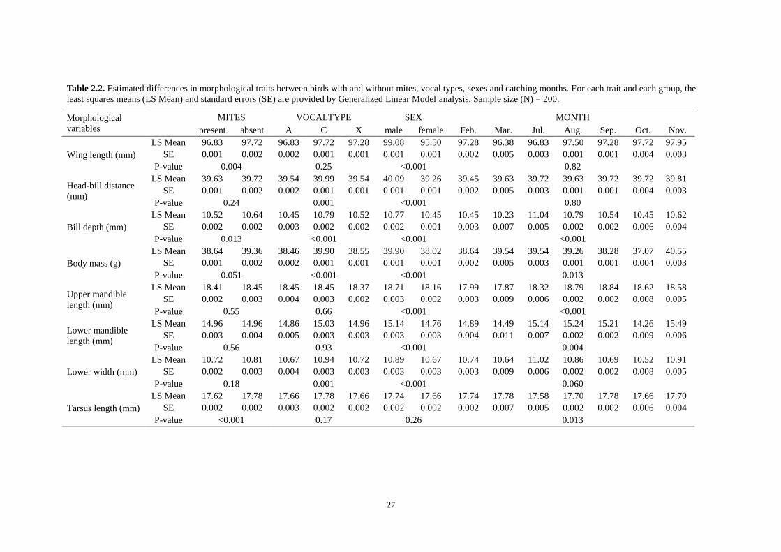
Univariate GLM’s was performed to show the influences of mite infestation, sex,

vocal type and month, on the eight morphological traits given as Table 2.2. The

corresponding p-value less than 0.05 implies that there is sufficient evidence against

the null hypothesis, that is, the candidate variable should be considered for the

relationship with the morphological trait(s). Overall, each of the explanatory variables

was significantly related to at least half the morphological dependent variables.

Logistic regression analysis shows that wing length and vocal type have a significant

effect on mite infestation, with a near-significant effect of tarsus length. According to

the output of binary LOGIT analysis, the variable of wing length most significantly

differs between crossbills with and without mites (P = 0.016), then vocal type is the

second (A: P = 0.075, C: P = 0.009), and ln-transformed tarsus length (P = 0.079) is

the third and near-significant variable in the optimal model, with the presented log-

likelihood as follows: LL(0) = -112.467, 2*[LL(N)-LL(0)] = 16.140 (d.f. = 4, P =

0.003). After estimating our model by logistic regression, we still considered month

and sex to have certain impact on mite infestation risk, so that these two variables

were added as a new model, which was compared with the former one. Change in

likelihood-ratio was 11.044 (d.f. = 7, P = 0.28), so there is no need to improve the

model by adding new factors. Therefore, wing length, tarsus length and vocal type are

other independent variables in the final model explaining mite infestation. Fig. 2.1-2.3

illustrate how the probability of mite infestation increases with the length of wings

and tarsi, and the pattern in Fig. 2.2 shows the probability of mites related with wing

length per vocal type in crossbills.

27

Table 2.2. Estimated differences in morphological traits between birds with and without mites, vocal types, sexes and catching months. For each trait and each group, the

least squares means (LS Mean) and standard errors (SE) are provided by Generalized Linear Model analysis. Sample size (N) = 200.

Morphological

variables

MITES VOCALTYPE SEX MONTH

present absent A C X male female Feb. Mar. Jul. Aug. Sep. Oct. Nov.

Wing length (mm)

LS Mean 96.83 97.72 96.83 97.72 97.28 99.08 95.50 97.28 96.38 96.83 97.50 97.28 97.72 97.95

SE 0.001 0.002 0.002 0.001 0.001 0.001 0.001 0.002 0.005 0.003 0.001 0.001 0.004 0.003

P-value 0.004 0.25 <0.001 0.82

Head-bill distance

(mm)

LS Mean 39.63 39.72 39.54 39.99 39.54 40.09 39.26 39.45 39.63 39.72 39.63 39.72 39.72 39.81

SE 0.001 0.002 0.002 0.001 0.001 0.001 0.001 0.002 0.005 0.003 0.001 0.001 0.004 0.003

P-value 0.24 0.001 <0.001 0.80

Bill depth (mm)

LS Mean 10.52 10.64 10.45 10.79 10.52 10.77 10.45 10.45 10.23 11.04 10.79 10.54 10.45 10.62

SE 0.002 0.002 0.003 0.002 0.002 0.002 0.001 0.003 0.007 0.005 0.002 0.002 0.006 0.004

P-value 0.013 <0.001 <0.001 <0.001

Body mass (g)

LS Mean 38.64 39.36 38.46 39.90 38.55 39.90 38.02 38.64 39.54 39.54 39.26 38.28 37.07 40.55

SE 0.001 0.002 0.002 0.001 0.001 0.001 0.001 0.002 0.005 0.003 0.001 0.001 0.004 0.003

P-value 0.051 <0.001 <0.001 0.013

Upper mandible

length (mm)

LS Mean 18.41 18.45 18.45 18.45 18.37 18.71 18.16 17.99 17.87 18.32 18.79 18.84 18.62 18.58

SE 0.002 0.003 0.004 0.003 0.002 0.003 0.002 0.003 0.009 0.006 0.002 0.002 0.008 0.005

P-value 0.55 0.66 <0.001 <0.001

Lower mandible

length (mm)

LS Mean 14.96 14.96 14.86 15.03 14.96 15.14 14.76 14.89 14.49 15.14 15.24 15.21 14.26 15.49

SE 0.003 0.004 0.005 0.003 0.003 0.003 0.003 0.004 0.011 0.007 0.002 0.002 0.009 0.006

P-value 0.56 0.93 <0.001 0.004

Lower width (mm)

LS Mean 10.72 10.81 10.67 10.94 10.72 10.89 10.67 10.74 10.64 11.02 10.86 10.69 10.52 10.91

SE 0.002 0.003 0.004 0.003 0.003 0.003 0.003 0.003 0.009 0.006 0.002 0.002 0.008 0.005

P-value 0.18 0.001 <0.001 0.060

Tarsus length (mm)

LS Mean 17.62 17.78 17.66 17.78 17.66 17.74 17.66 17.74 17.78 17.58 17.70 17.78 17.66 17.70

SE 0.002 0.002 0.003 0.002 0.002 0.002 0.002 0.002 0.007 0.005 0.002 0.002 0.006 0.004

P-value <0.001 0.17 0.26 0.013

28

Fig. 2.1. Simulation of probability of mites related to wing length. The 95% confidential interval is

given by vertical bars. Tarsus length was fixed at the overall mean of log(tarsus length) = 1.248.

Fig. 2.2. Simulation of probability of mites related to wing length per vocal type. (C.I.=0.95)

0.0

0.1

0.2

0.3

0.4

0.5

0.6

0.7

0.8

0.9

1.0

Pro

ba

bil

ity o

f M

ite

s

Wing length (log)

Average

probability

0.0

0.1

0.2

0.3

0.4

0.5

0.6

0.7

0.8

0.9

1.0

Wing length (log)

Pro

ba

bil

ity o

f M

ite

s

A

C

X

29

Fig. 2.3. Simulation of probability of mites related to tarsus length. The variable wing length was fixed

at the overall mean of log(wing length) = 1.988.

0.0

0.1

0.2

0.3

0.4

0.5

0.6

0.7

0.8

0.9

1.0

Average

probability

Pro

ba

bil

ity o

f M

ite

s

Tarsus length (log)

30

Discussion

It is an interesting issue in evolutionary biology to study the morphological

differentiation caused by selection forces. In this section, the infestation of mites,

which can depress birds’ survival for damage to host health or reproductive fitness

(Proctor and Owens 2000), is considered a selection force driving adaptation radiation

of crossbills. Mites may also transmit viral diseases among birds besides have direct

effect upon their hosts, and it appears that larger crossbills are prone to be infected by

mites compared with smaller ones. So our hypothesis is that mite infestation may

cause directional selection against individuals with larger body sizes, specifically

longer wings.

The first aim of our study is to test if any categorical variables (mite infection, sex,

vocal type and catching month) are significantly related to each morphological trait

(wing length, mass, head-bill distance, bill depth, upper mandible length, lower

mandible length, and lower mandible width). Therefore, as the first step, univariate

morphological differences between crossbills grouped by categorical variables were

identified by GLM method for each of the measured traits. The results indicate that, of

the explanatory variables, vocal type may have an impact on head-bill distance, bill

depth and lower mandible width; sex influences almost all the variables (males are

larger); bill depth, mass, lower mandible length, lower mandible width, and tarsus

length seem to vary among crossbills trapped in different months (Table 2.2). Then,

from the results of logistic regression analysis, the length of wings seems to differ

most significantly between the crossbills with and without mites, suggesting that

mites could cause directional selection on wing length. This makes sense in respect

that the wing length is closely related to body size, which is more likely to be the

target of mite selection (Benkman et al. 2005). Referring to the length of tarsus, it is

significantly correlated with both wing length and weight in many species of birds

such as Citril Finch (Alonso and Arizaga 2006), providing a good predictor of avian

body size.

We also wondered if prevalence of mite infestation differed among various crossbill

vocal types, so logistic regression and simulation analyses on probability of mites

related with wing length per vocal type (Fig. 2.2) were performed. The trends of

infection risk probability are rising with increase of wing length for all three vocal

types. The curve of vocal type A seems to stand out a bit, possibly due to the limited

sample size which reduces statistical power. Nevertheless, it is clear that the

probabilities of infestation by mites differ between three vocal types. This discovery is

exciting since vocal type was not a highlight regarded to have a relationship with

mites, for example, all the individuals were of the South Hill vocal type in Benkman’s

study (Benkman et al. 2005). Although the difference caused by mites mentioned

above may be not with extraordinary power of influence in the evolutionary history of

crossbills, it could have an impact on the pattern considering vocal type used as a

31

means to discriminate crossbill populations..

We also considered whether the occurrence of infection by scaly-leg mites were

associated with other factors. The incidence of mites among adult South Hills

crossbills fluctuated in time from 1997 and 2004 (Benkman et al. 2005), implying it

could also vary among catching year. Besides, male crossbills were potentially more

inclined to display symptoms of scaly-leg mites than were females based on the

research about sex-biases in the occurrence and severity of parasites in populations of

mammals (Moore and Wilson 2002). The relatively low level of sexual size

dimorphism in South Hills crossbills compared to others suggested recent selection by

ectoparasitic mites and direct selection against larger-billed male crossbills (Benkman

et al. 2005). However, no straightforward evidence was provided to indicate the

interaction between sex and morphology in Benkman’s study. They used logistic

regressions and linear regressions analyses separately to determine if the incidence of

mites varied in relation to sex factor and capture year and if the bill depth varied

linearly across years. But t-tests was used to determine if birds with and without mites

differed in bill depth grouped by sex instead of directly including the factor of sex in

the regression analyses. Therefore, to figure out the relationship between bill size and

sex or other factors more clearly, we used logistic regression analysis to test the model

combining all the morphological variables and the factors sex, vocal type and

catching month in one joint analysis. The final model is specified that the presence of

mites is significantly related to wing length and vocal type, and almost significantly to

tarsus length. Besides, the result confirms that mites do not affect sexual size-

dimorphism of crossbills directly and suggests that there is a direct link between mite

selection and morphological traits of bills rather than indirect selection.

In brief, our study in this section highlights the directional selection caused by scaly-

leg mites over the morphology of crossbills, including the length of wings and tarsi. In

addition, infections differ between vocal types, implying that mites could distribute

the evolutionary patterns in the adaptive radiation of crossbills.

32

Conclusion

To conclude, we firstly detected divergent natural selection potentially caused by use

of resource by comparison of neutral genetic differentiation at marker loci and

quantitative traits among crossbill populations. And then we confirm that wing length

and tarsus length affect the prevalence of infestation by scaly-leg mites and suggest

that mites could cause morphological differentiation of vocal types because vocal

types differ significantly in infection rate. In summary, combining these two parts of

studies, we find support for the hypothesis that resource use can drive the adaptive

radiation of crossbill morphology, but other selective forces such as scaly-leg mites

can confound evolutionary patterns.

33

Acknowledgements

I would like to express my gratitude to all those who gave me the possibility and

support to complete this thesis. I am grateful to my supervisors Dr. Pim Edelaar, Dr.

Reija Dufva and Prof. Mats Björklund for their self-giving help and patient training.

Especially, I am deeply indebted to Pim for his kindness and wisdom to encourage my

scientific thoughts. I also thank Prof. Jacob Höglund, Prof. Håkan Rydin, Dr. Niclas

Backström, Candice Andersson, Pontus Skoglund, Michael Stocks, Eleftheria

Palkopoulou, Padraicgerard Corcoran, Xiaomeng Li, Shuang Gao, Jingzhi Hu, Hao

Luo and Hongyi Zhao, who gave me a lot of valuable suggestions and awesome

memories in my master studies. Thanks to all the people in the Department of Animal

Ecology for sharing scientific ideas and happy hours.

Many thanks to my family and all the other friends whose brilliant love enabled me to

complete this work and enjoyed my life!

34

References

Alonso, D. and Arizaga, J. 2006. Biometrics of Citril Finch Serinus citrinella in

the west Pyrenees and the influence of feather abrasion on biometric data. Ringing &

Migration 23: 116-124.

Altaba, C.R. 2001. Un endemisme ornitologic ignorat: el trencapinyons balear

(Loxia balearica). Butll. Inst. Cat. Hist. Nat. 69: 77–90.

Benkman, C. W. 1993. Adaptation to single resources and the evolution of

crossbill (Loxia) diversity. Ecol. Monogr. 63: 305–325.

Benkman, C.W. and Miller, R. E. 1996. Morphological evolution in response

to fluctuating selection. Evolution 50: 2499-2504.

Benkman, C. W. 1999. The selection mosaic and diversifying coevolution

between crossbills and lodgepole pine. American Naturalist 154: S75-S91.

Benkman, C. W. 2003. Divergent selection drives the adaptive radiation of

crossbills. Evolution 57: 1176-1181.

Benkman, C.W., Colquitt, J.S., Gould, W.R., Fetz, T., Keenan, P.C. and

Santisteban, L. 2005. Can selection by an ectoparasite drive a population of red

crossbills from its adaptive peak? Evolution 59: 2025-2032.

Borrás, A., Cabrera, J. and Senar, J.C. 2008. Local divergence between

Mediterranean crossbills occurring in two different species of pine. Ardeola 55(2):

169-177.

Cramp, S. 7 Perrins, C.M. 1994. The birds of the Western Palearctic. Oxford

University Press 8: 894

Edelaar, P., Summers, R. and Iovchenko, N. 2003. The ecology and evolution

of crossbills Loxia spp.: the need for a fresh look and an international research

program. Avian Sci. 3: 85–93.

Edelaar, P. 2008. Rediscovery of a second kind of crossbill for The Himalayan

region, and the hypothesis that ecological opportunity drives crossbill diversification.

Ibis 150: 405-408.

Hedrick, P. W. 1999. Perspective: highly variable loci and their interpretations

in evolution and conservation. Evolution 53: 313–318.

James, H. F. 2004. The osteology and phylogeny of the Hawaiian finch radiation

(Fringillidae: Drepanidini), including extinct taxa. Zoological Journal of the Linnean

Society 141: 207–255.

Klenerman, P. and Lipworth, B. 2008. House dust mite allergy.

Lande, R. 1976. Natural selection and random genetic drift in phenotypic

evolution. Evolution 30: 314–334.

Lynch, M. 1990. The rate of morphological evolution in mammals from the

standpoint of the neutral expectation. Am. Nat 136: 727–741.

Latta, R.G. 1998. Differentiation of allelic frequencies at quantitative trait loci

affecting locally adaptive traits. American Naturalist 151: 293-292.

Latta, S. C. and J. Faaborg. 2001. Winter site fidelity of Prairie Warblers in the

Dominican Republic. Condor 103: 455-468.

35

Latta, S. C. 2003. Effects of scaley-leg mite infestations on body condition and

site fidelity of migratory warblers. Auk 120: 730-743.

Lessells, C. M. and P. T. Boag. 1987. Unrepeatable repeatabilities: A common

mistake. Auk 104: 116–121.

Massa, B. 1987. Variations in Mediterranean crossbills Loxia curvirostra. Bull

Brit Ornith Club 107: 118–29

Merilae, J. and Crnokrak, P. 2001. Comparison of genetic differentiation at

marker loci and quantitative traits. J. Evol. Biol. 14: 892-903.

Mezquida E.T. and Benkman C.W. 2005. The geographic selection mosaic for

squirrels, crossbills and Aleppo pine. J. Evol. Biol. 18: 348–357.

Moore, S. L. and Wilson, K. 2002. Parasites as a viability cost of sexual

selection in natural populations of mammals. Science 297: 2015–2018.

Pence, D. B., Cole, R. A., Brugger, K. E., and Fischer, J. R. 1999. Epizootic

podoknemidokoptiasis in American robins. Journal of wildlife diseases 35: 1-7.

Proctor, H.C. and I. Owens. 2000. Mites and birds: diversity, parasitism and

coevolution. Trends in Ecology and Evolution 15: 358-364.

Pujol, B., Wilson, A.J, Ross, R.I.C., Pannell, J.R. 2008. Are QST-FST

comparisons for natural populations meaningful? Molecular Ecology. 17(22): 4782-

4785.

Richardson, D. M. 1998. Forestry trees as invasive aliens. Conserv. Biol 12:

18–26.

Robb, M. 2000. Introduction to vocalizations of crossbills in north-western

Europe. Dutch Birding 22: 61–107.

Rogers, A. 1986. Population differences in quantitative characters as opposed to

gene frequencies, Am. Nat. 127: 729–730.

Schluter, D. 2000.The Ecology of Adapative Radiation. Oxford University Press,

New York.

Senar, J. C., Borrás, A., Cabrera, T. and Cabrera, J. 1993. Testing for the

relationship between coniferous crops stability and common crossbills residence. J

Field Ornitho 64: 464–469.

Spitze, K. 1993. Population structure in Daphnia obtusa: quantitative genetics

and allozymic variation. Genetics 135: 367–374.

Summers, R. W., Dawson, R. J. and Phillips, R. E. 2007. Assortative mating

and patterns of inheritance indicate that the three crossbill taxa in Scotland are species.

J. Avian Biol. 38: 153–162.

Whitlock, M. C. 2008 Evolutionary inference from QST. Mol. Ecol. 17: 1885–

1896.