testing endogeneity with possibly invalid … endogeneity with possibly invalid instruments and high...
TRANSCRIPT

Testing Endogeneity with Possibly Invalid
Instruments and High Dimensional Covariates
Zijian Guo, Hyunseung Kang, T. Tony Cai and Dylan S. Small
Abstract
The Durbin-Wu-Hausman (DWH) test is a commonly used test forendogeneity in instrumental variables (IV) regression. Unfortunately,the DWH test depends, among other things, on assuming all the instru-ments are valid, a rarity in practice. In this paper, we show that theDWH test often has distorted size even if one IV is invalid. Also, theDWH test may have low power when many, possibly high dimensional,covariates are used to make the instruments more plausibly valid. Toremedy these shortcomings, we propose a new endogeneity test whichhas proper size and better power when invalid instruments and highdimemsional covariates are present; in low dimensions, the new testis optimal in that its power is equivalent to the “oracle” DWH test’spower that knows which instruments are valid. The paper concludeswith a simulation study of the new test with invalid instruments andhigh dimensional covariates.
1 Introduction
Many empirical studies using instrumental variables (IV) regression are ac-companied by the Durbin-Wu-Hausman test [Durbin, 1954, Wu, 1973, Haus-man, 1978], hereafter called the DWH test. The primary purpose of theDWH test is to test the presence of endogeneity by comparing the ordinaryleast squares (OLS) estimate of the structural parameters in the IV regres-sion to that of the two-stage least squares (TSLS). Consequently, the DWHtest is often used to decide whether to use an IV analysis compared to a stan-dard OLS analysis; the IV analysis has lower bias when the included pos-sibly endogenous variable in the IV regression is truly endogenous whereas
1

the standard OLS analysis has smaller variance [Davidson and MacKinnon,1993].
Properly using the DWH test depends, among other things, on havinginstruments that are (i) strongly associated with the endogenous variable,often called strong instruments, and are (ii) known, with absolute certainty,to be exogenous1, often referred to as valid instruments [Murray, 2006]. Forexample, when instruments are not strong, Staiger and Stock [1997] showedthat the DWH test that used the TSLS estimator for variance, which is at-tributed to Durbin [1954] and Wu [1973], had distorted size under the nullhypothesis while the DWH test that used the OLS estimator for variance,which is attributed to Hausman [1978], had proper size. Unfortunately,when instruments are not valid, which is perhaps a bigger concern in prac-tice [Murray, 2006, Conley et al., 2012] and has arguably received far lessattention than when the instruments are weak, there is a paucity of workon exactly characterizing the behavior of the DWH test. Also, with largedatasets becoming more prevalent, there has been a trend toward condition-ing on many, possibly high dimensional, exogenous covariates in structuralmodels to make instruments more plausibly valid2 [Gautier and Tsybakov,2011, Belloni et al., 2012, Chernozhukov et al., 2015]. However, it’s unclearhow the DWH test is affected in the presence of many covariates. Moreimportantly, even after conditioning, some IVs may still be invalid and sub-sequent analysis, including the DWH test, assuming that all the IVs arevalid after conditioning can be misleading.
Prior work in analyzing the DWH test in instrumental variables is di-verse. Estimation and inference under weak instruments are well-documented[Staiger and Stock, 1997, Nelson and Startz, 1990, Bekker, 1994, Boundet al., 1995, Dufour, 1997, Zivot et al., 1998, Wang and Zivot, 1998, Kleiber-gen, 2002, Moreira, 2003, Chao and Swanson, 2005, Andrews et al., 2007].In particular, when the instruments are weak, the behavior of the DWHtest under the null depends on the variance estimate [Staiger and Stock,1997, Nakamura and Nakamura, 1981, Doko Tchatoka, 2015]. Some recent
1The term exogeneity is sometimes used in the IV literature to encompass two as-sumptions, (a) independence of the IVs to the disturbances in the structural model and(b) IVs having no direct effect on the outcome, sometimes referred to as the exclusionrestriction [Holland, 1988, Imbens and Angrist, 1994, Angrist et al., 1996]. As such, aninstrument that is perfectly randomized from a randomized experiment may not be exoge-nous in the sense that while the instrument is independent to any structural error terms,the instrument may still have a direct effect on the outcome.
2For example, in causal inference and epidemiology, Hernan and Robins [2006] andBaiocchi et al. [2014] highlights the need to control for covariates for an instrument toremove violations of exogeneity.
2

work extends the specification test to handle growing number of instruments[Hahn and Hausman, 2002, Chao et al., 2014]. Unfortunately, all these workshave not characterized the properties of the DWH test when instruments areinvalid.
In addition, there is a growing literature on estimation and inference ofstructural effects in high dimensional instrumental variables models [Gau-tier and Tsybakov, 2011, Belloni et al., 2012, Chernozhukov et al., 2015,Belloni et al., 2011a, 2013, Fan and Liao, 2014, Chernozhukov et al., 2014].Unfortunately, all of them assume that after controlling for high dimensionalcovariates, all the IVs are valid, which may not be true in practice.
Finally, for work related to invalid instruments, Fisher [1966, 1967],Newey [1985], Hahn and Hausman [2005], Guggenberger [2012], Berkowitzet al. [2012] and Caner [2014] considered properties of IV estimators or,more broadly, generalized method of moments estimators (GMM)s whenthere are local deviations from validity to invalidity. Andrews [1999] andAndrews and Lu [2001] considered selecting valid instruments within thecontext of GMMs. Small [2007] approached the invalid instrument problemvia a sensitivity analysis. Conley et al. [2012] proposed various strategies,including union-bound correction, sensitivity analysis, and Bayesian analy-sis, to deal with invalid instruments. Liao [2013] and Cheng and Liao [2015]considered the setting where there is, a priori, a known set of valid instru-ments and another set of instruments that may not be valid. Recently, Kanget al. [2016] and Kolesar et al. [2015] worked under the case where this a pri-ori information is absent. Kang et al. [2016] replaced the a priori knowledgewith a sparsity-type assumption on the number of invalid instruments whileKolesar et al. [2015] replaced the a priori knowledge with an orthogonalityassumption on the instruments’ effects on the included endogenous variableand the outcome. In all cases, the main focus was on the selection of validinstruments or the estimation of structural parameters; none of the authorsconsidered studying the properties of the endogeneity test.
Our main contribution is two-fold. First, we expand the theoretical anal-ysis of the DWH test under weak instruments by showing negative resultsabout the DWH test under invalid instruments and high dimensional co-variates. We show that the DWH test fails to have the correct size in thepresence of invalid instruments and we precisely characterize the deviationfrom the nominal level. We also show that the DWH test has low powerwhen many covariates are present, especially when the number of covariatesis similar to the sample size. Second, we remedy the failures of the DWHtest by presenting an improved endogeneity test that is robust to both in-valid instruments and high dimensional covariates and that works in settings
3

where the number of structural parameters exceed the sample size. The keyidea behind the new endogeneity test is based on a novel methodology thatwe call two-stage hard thresholding (TSHT) which allows selection of validinstruments and subsequent inference after selection. In the low dimensionalsetting, we show that our new test has optimal performance in that our testhas the same asymptotic power as the “oracle” DWH test that knows whichinstruments are valid and invalid. In the high dimensional setting, we char-acterize the asymptotic power of the new proposed test and show that thepower of the new test is better than the DWH test. We conclude the paperwith simulation studies comparing the performance of our new test with theDWH test. We find that our test has the desired size and has better powerthan that of the DWH test when invalid instruments and high dimensionalcovariates are present. We also present technical proofs and extended simu-lation studies that further examine the power and sensitivity of our test toregularity assumptions in the supplement.
2 Instrumental Variables Regression and the DWHTest
2.1 Notation
For any p dimensional vector v, the jth element is denoted as vj . Let ‖v‖1,‖v‖2, and ‖v‖∞ denote the 1, 2 and ∞-norms, respectively. Let ‖v‖0 denotethe number of non-zero elements in v and let supp(v) = j : vj 6= 0 ⊆1, . . . , p. For any n by p matrix M , denote the ith row and jth columnentry as Mij , the ith row vector as Mi., the jth column vector as M.j ,and M ′ as the transpose of M . Also, given any n by p matrix M withsets I ⊆ 1, . . . , n and J ⊆ 1, . . . , p denote MIJ as the submatrix of Mconsisting of rows specified by the set I and columns specified by the set J .Let ‖M‖∞ represent the element-wise matrix sup norm of matrix M . Also,for any n× p full-rank matrix M , define the orthogonal projection matricesPM = M(M ′M)−1M ′ and PM⊥ = I−M(M ′M)−1M ′ where PM +PM⊥ = Iand I is an identity matrix. For a p × p matrix Λ, Λ 0 denotes thatΛ is a positive definite matrix. For any p × p positive definite Λ and setJ ⊆ 1, . . . , p, let ΛJ |JC = ΛJJ − ΛJJCΛ−1
JCJCΛJCJ denote the submatrixΛJJ adjusted for the columns Jc.
For a sequence of random variables Xn indexed by n, we use Xnp→ X to
represent that Xn converges to X in probability. For a sequence of randomvariables Xn and numbers an, we define Xn = op(an) if Xn/an converges
4

to zero in probability and Xn = Op(an) if for every c0 > 0, there exists afinite constant C0 such that P (|Xn/an| ≥ C0) ≤ c0. For any two sequencesof numbers an and bn, we will write bn an if lim sup bn/an = 0.
For distribution of random variables, for any α, 0 < α < 1, and B ∈ R,we define
G(α,B) = 1− Φ(zα/2 −B) + Φ(−zα/2 −B) (1)
where Φ and zα/2 are respectively the cumulative distribution function andα/2 quantile of a standard normal distribution. We also denote χ2
α(d) to bethe 1−α quantile of the chi-squared distribution with d degrees of freedom.
2.2 Model and Definitions
Suppose we have n individuals where for each individual i = 1, . . . , n, wemeasure the outcome Yi, the included endogenous variable Di, pz candidateinstruments Z ′i., and px exogenous covariates X ′i. in an i.i.d. fashion. Wedenote W ′i. to be concatenated vector of Z ′i. and X ′i. and the correspondingdimension of Wi. to be p = pz + px. The matrix W is indexed by the setI = 1, . . . , pz which consists of all the pz candidate instruments and theset IC = pz + 1, . . . , p which consists of the px covariates. The variables(Yi, Di, Zi, Xi) are governed by the following structural model
Yi = Diβ + Z ′i.π +X ′i.φ+ δi, E(δi | Zi., Xi.) = 0 (2)
Di = Z ′i.γ +X ′i.ψ + εi, E(εi | Zi., Xi.) = 0 (3)
where β, π, φ, γ, and ψ are unknown parameters in the model and withoutloss of generality, we assume the variables are centered to mean zero3. Therandom disturbance terms δi and εi are independent of (Zi., Xi.) and, for sim-plicity, are assumed to be bivariate normal. Let the population covariancematrix of (δi, εi) be Σ, with Σ11 = Var(δi|Zi., Xi.), Σ22 = Var(εi|Zi., Xi.),and Σ12 = Σ21 = Cov(δi, εi|Zi., Xi.). Let the second order moments of Wi.
be Λ = E (Wi·W′i·) with ΛI|Ic as the adjusted covariance of Wi.. Let ω
represent all the parameters ω = (β, π, φ, γ, ψ,Σ) from the parameter spaceω ∈ Ω = R⊗Rpz⊗Rpx⊗Rpz⊗Rpz⊗Σ 0. Finally, we denote sz2 = ‖π‖0,sx2 = ‖φ‖0, sz1 = ‖γ‖0, sx1 = ‖ψ‖0 and s = maxsz2, sx2, sz1, sx1.
If π = 0 in model (2), the models (2) and (3) represent the usual in-strumental variables regression models with one endogenous variable, pxexogenous covariates, and pz instruments, all of which are assumed to bevalid. On the other hand, if π 6= 0 and the support of π is unknown a priori,
3The mean-centering is equivalent to adding a constant 1 term (i.e. intercept term) inX ′i.
5

the instruments may have a direct effect on the outcome, thereby violatingthe exclusion restriction [Imbens and Angrist, 1994, Angrist et al., 1996] andmaking them potentially invalid, without knowing, a priori, which are in-valid and valid [Murray, 2006, Conley et al., 2012, Kang et al., 2016]. In fact,among pz candidate instruments, the support of π allows us to distinguisha valid instrument from an invalid one and provides us with a definition ofa valid instrument.
Definition 1. Suppose we have pz candidate instruments along with themodel (2). We say that instrument j = 1, . . . , pz is valid if πj = 0 andinvalid if πj 6= 0.
In addition, it is also useful to define relevant instruments from theirrelevant instruments. This is, in many ways, equivalent to the notion thatthe instruments Zi. are associated with the endogenous variable Di, exceptlike Definition 1, we use the support of a vector to define the instruments’association to the endogenous variable; see Breusch et al. [1999], Hall andPeixe [2003], and Cheng and Liao [2015] for some examples in the literatureof defining relevant and irrelevant instruments based on the support of aparameter.
Definition 2. Suppose we have pz instruments along with the model (3).We say that instrument j = 1, . . . , pz is relevant if γj 6= 0 and irrelevant ifγj = 0. Let S be the set of relevant instruments.
Definitions 1 and 2 combine to form valid and relevant instruments. Wedenote the set of instruments that satisfy both definitions as V = j | πj =0, γj 6= 0. Note that Definitions 1 and 2 are related to the definition ofinstruments that is well known in the literature. In particular, if pz = 1,an instrument that is relevant and valid is identical to the definition ofan instrument in Holland [1988]. In particular, Definition 1 is the sameas ignorability and exclusion restriction while Definition 2 is the same asthe condition that the instrument is related to the exposure. Definitions 1and 2 are also a special case of a definition of an instrument discussed inAngrist et al. [1996] where in our setup, we assume an additive, linear, and aconstant treatment effect model. Hence, when multiple instruments, pz > 1,are present, Definitions 1 and 2, especially Definition 1, can be viewed as ageneralization of the definition of an instrument in the pz = 1 case.
In the literature, Kang et al. [2016] considered the aforementioned frame-work and Definition 1 as a relaxation of instrumental variables assumptionswhere a priori information about which of the pz instruments are valid or
6

invalid is not available and provided sufficient and necessary conditions foridentification of β. Guo et al. [2016] expanded the work in Kang et al. [2016]by allowing high dimensional covariates and instruments along with deriv-ing honest confidence intervals for β. Kolesar et al. [2015] also analyzed themodels (2) and (3) in the presence of invalid instruments, but they assumedorthogonality restrictions between π and γ.
Finally, for the set of valid and relevant IVs V, we define the concentra-tion parameter, a common measure of instrument strength,
C(V) =γ′VΛV|VCγV
|V|Σ22. (4)
If all instruments were relevant and valid, then V = I and equation (4) isthe usual definition of concentration parameter in Staiger and Stock [1997],Bound et al. [1995], Mariano [1973], Stock and Wright [2000] using popula-tion quantities, i.e. ΛV|VC . 4 However, if only a subset of all instruments arerelevant and valid so that V ⊂ 1, . . . , pz, then the concentration parameterrepresents the strength of the instruments for that subset V, adjusted for theinstruments in its complement VC = 1, . . . , pz, pz + 1, . . . , p \ V. Regard-less, like the usual concentration parameter, a high value of C(V) representsstrong instruments in the set V while a low value of C(V) represents weakinstruments.
2.3 The DWH Test
Consider the following hypotheses for endogeneity in models (2) and (3),
H0 : Σ12 = 0, H1 : Σ12 6= 0, (5)
The DWH test tests for endogeneity as specified by the hypothesis in equa-tion (5) by comparing two consistent estimators of β under the null hy-pothesis H0, i.e. no endogeneity, with different efficiencies. Specifically, theDWH test statistic, denoted as QDWH, is the quadratic difference of the theOLS estimate of β, denoted as βOLS = (D′PX⊥D)−1D′PX⊥Y , and the TSLSestimate of β, denoted as βTSLS = (D′(PW − PX)D)−1D′(PW − PX)Y,
QDWH =(βTSLS − βOLS)2
Var(βTSLS)− Var(βOLS)(6)
4For example, if V = I so that all IVs are valid, C(V) corresponds exactly to the quan-tity λ′λ/K2 on page 561 of Staiger and Stock [1997] for n = 1 and K1 = 0. Without usingpopulation quantities, nC(V) roughly corresponds to the usual concentration parameterusing the estimated version of ΛV|VC
7

where Var(βOLS) = (D′PX⊥D)−1 Σ11, Var(βTSLS) = (D′(PW − PX)D)−1 Σ11,and Σ11 can either be the OLS estimate of Σ, i.e. Σ11 = ‖Y − DβOLS −XφOLS‖22/n, or the TSLS estimate of Σ, i.e. Σ11 = ‖Y−DβTSLS−XφTSLS‖22/n5.Under H0, both OLS and TSLS are consistent estimates of β, but the OLSestimate is more efficient than TSLS. Also, under H0, both OLS and TSLSestimates of the variance Σ11 are consistent.
If π = 0 so that all the instruments are valid, the asymptotic null distri-bution of the DWH test in equation (6) is Chi-squared with one degree offreedom. With a known Σ11, the DWH test has an exact Chi-squared nulldistribution with one degree of freedom. Regardless, both null distributionsimply that for α, 0 < α < 1, we can reject the null hypothesis H0 for thealternative H1 by using the decision rule,
Reject H0 if QDWH ≥ χ2α(1)
and the Type I error of the DWH test will be exactly or asymptoticallycontrolled at level α. Also, under the local alternative hypotheses,
H0 : Σ12 = 0, H2 : Σ12 =∆1√n
(7)
for some constant ∆1, the asymptotic power of the DWH test is
ω ∈ H2 : limn→∞
P(QDWH ≥ χ2α(1)) = G
α, ∆1
√C(I)√(
C(I) + 1pz
)Σ11Σ22
. (8)
For more information about the DWH test, see Davidson and MacKinnon[1993] and Wooldridge [2010] for textbook discussions.
3 Failure of the DWH Test
3.1 Invalid Instruments
While the DWH test performs as expected when all the instruments arevalid, in practice, some instruments may be invalid and consequently, theDWH test can be a highly misleading assessment of the hypotheses (5). InTheorem 1, we show that the Type I error of the DWH test can be greater
5To be precise, the OLS and TSLS estimates of φ can be obtained as follows: φOLS =(X ′PD⊥X)−1X ′PD⊥Y and φTSLS = (X ′PD⊥X)−1X ′PD⊥Y where D = PWD.
8

than the nominal level for a wide range of IV configurations in which someIVs are invalid; we assume a known Σ11 in Theorem 1 for a cleaner technicalexposition and to highlight the impact that invalid IVs have on the size andpower of the DWH test, but the known Σ11 can be replaced by a consistentestimate of Σ11. We also show that the power of the DWH test under thelocal alternative H2 in equation (7) can be shifted.
Theorem 1. Suppose we have models (2) and (3) with a known Σ11. Ifπ = ∆2/n
k where ∆2 is a fixed constant and 0 ≤ k < ∞, then for any α,0 < α < 1, we have the following asymptotic phase-transition behaviors ofthe DWH test for different values of k.
a. 0 ≤ k < 1/2: The asymptotic Type I error of the DWH test under H0
is 1, i.e.ω ∈ H0 : lim
n→∞P(QDWH ≥ χ2
α(1))
= 1 (9)
and subsequently, the asymptotic power of the DWH test under H2 is1.
b. k = 1/2: The asymptotic Type I error of the DWH test under H0 is
ω ∈ H0 : limn→∞
P(QDWH ≥ χ2
α(1))
= G
α, 1pzγ′ΛI|Ic∆2√
C(I)(C(I) + 1
pz
)Σ11Σ22
≥ α(10)
and the asymptotic power of the DWH test under H2 is
ω ∈ H2 : limn→∞
P(QDWH ≥ χ2
α(1))
= G
α, 1pzγ′ΛI|Ic∆2√
C(I)(C(I) + 1
pz
)Σ11Σ22
+∆1
√C(I)√(
C(I) + 1pz
)Σ11Σ22
(11)
c. 1/2 < k <∞: The asymptotic Type I error of the DWH test is α, i.e.
ω ∈ H0 : limn→∞
P(QDWH ≥ χ2
α(1))
= α (12)
and the asymptotic power of the DWH test under H2 is equivalent toequation (8).
9
Theorem 1 presents the asymptotic behavior of the DWH test under awide range of behaviors for the invalid IVs as represented by π. For example,when the instruments are invalid in the sense that their deviation from validIVs (i.e. π = 0) to invalid IVs (i.e. π 6= 0) is at rates slower than n−1/2, sayπ = ∆2n
−1/4 or π = ∆2, equation (9) states that the DWH will always haveType I error that reaches 1. In other words, if some IVs, or even a single IV,are moderately (or strongly) invalid in the sense that they have moderate(or strong) direct effects on the outcome above the usual noise level of themodel error terms at n−1/2, then the DWH test will always reject the nullhypothesis of no endogeneity even if there is truly no endogeneity present.
Next, suppose the instruments are invalid in the sense that their devia-tion from valid IVs to invalid IVs are exactly at n−1/2 rate, also referred toas the Pitman drift.6 This is the phase-transition point of the DWH test’sType I error as the error moves from 1 in equation (9) to α in equation (12).Under this type of invalidity, equation (10) shows that the Type I error of theDWH test depends on some factors, most prominently the factor γ′ΛI|Ic∆2.The factor γ′ΛI|Ic∆2 has been discussed in the literature, most recently byKolesar et al. [2015] within the context of invalid IVs. Specifically, Kolesaret al. [2015] studied the case where ∆2 6= 0 so that there are invalid IVs, butγ′ΛI|Ic∆2 = 0, which essentially amounted to saying that the IVs’ effecton the endogenous variable D via γ is orthogonal to their direct effects onthe outcome via ∆2; see Assumption 5 of Section 3 in Kolesar et al. [2015]for details. Under their scenario, if γ′ΛI|Ic∆2 = 0, then the DWH test willhave the desired size α. However, if γ′ΛI|Ic∆2 is not exactly zero, which willmost likely be the case in practice, then the Type I error of the DWH testwill always be larger than α and we can compute the exact deviation from αby using equation (10). Also, equation 11 computes the power under H2 inthe n−1/2 setting, which again depends on the magnitude and direction ofγ′ΛI|Ic∆2. For example, if there is only one instrument and that instrumenthas average negative effects on both D and Y , the overall effect on the powercurve will be a positive shift away from the null value Σ12 = 0. Regardless,under the n−1/2 invalid IV regime, the DWH test will always have size thatis at least as large as α if invalid IVs are present.
Theorem 1 also shows that instruments’ strength, as measured by thepopulation concentration parameter C(I) in equation (4), impacts the Type
6Fisher [1967] and Newey [1985] have used this type of n−1/2 asymptotic argumentto study misspecified econometrics models, specifically Section 2, equation (2.3) of Fisher[1967] and Section 2, Assumption 2 of Newey [1985]. More recently, Hahn and Hausman[2005] and Berkowitz et al. [2012] used the n−1/2 asymptotic framework in their respectiveworks to study plausibly exogenous variables.
10

I error rate of the DWH test when the IVs are invalid at the n−1/2 rate.Specifically, if π = ∆2n
−1/2 and the instruments are strong so that theconcentration parameter C(I) is large, then the deviation from α will berelatively minor even if γ′ΛI|Ic∆2 6= 0. This phenomena has been mentionedin previous work, most notably Bound et al. [1995] and Angrist et al. [1996]where strong instruments can lessen the undesirable effects caused by invalidIVs. However, if the invalidity is at a rate other than n−1/2, the strength ofthe IV has no impact on the Type I error of the DWH test. For instance, ifπ is slower than n−1/2 at π = ∆2n
−1/4, the Type I error rate of the DWHtest will always be 1 for any value of the concentration parameter.
Finally, if the instruments are invalid in the sense that their deviationfrom π = 0 is faster than n−1/2, say π = ∆n−1, then equation (12) showsthat the DWH test maintains its desired size. To put this invalid IV regime incontext, if the instruments are invalid at n−k where k > 1/2, the convergencetoward π = 0 is faster than the usual convergence rate of a sample mean froman i.i.d. sample towards a population mean. Also, this type of deviationis equivalent to saying that the invalid IVs are very weakly invalid andessentially act as if they are valid because the IVs are below the noise levelof the model error terms at n−1/2. Consequently, the DWH test is notimpacted by these type of IVs with respect to size and power.
In short, Theorem 1 shows that the DWH test can fail with regards tonot being able to control its Type I error. Indeed, the only cases when theDWH test achieves its desired size α are (i) when the invalid IVs essentiallybehave as valid IVs asymptotically, i.e. the case when 1/2 < k < ∞, and(ii) when the IVs’ effects on the endogenous variables are orthogonal to eachother. However, in all other cases, which are arguably more realistic, theDWH test will have Type I error that is strictly greater than α.
3.2 Large Number of Covariates
Next, we consider the behavior of the DWH test when the instruments areassumed to be valid after conditioning on many covariates. As noted inSection 1, many empirical studies often condition on covariates to makeinstruments more plausibly valid, with the likelihood of having valid IVsincreasing as one conditions on more covariates. Theoretically, this settingwas studied by Gautier and Tsybakov [2011], Belloni et al. [2012, 2011a,2013], Fan and Liao [2014], Chernozhukov et al. [2014] and Chernozhukovet al. [2015], who provided honest confidence intervals for a treatment effect,even in the case when the number of covariates and instruments exceededthe sample size. The authors have not studied the behavior of the DWH test
11
under this scenario, specifically the effect on the DWH test by having manycovariates to make IVs valid. As we will see below, a tradeoff of having morecovariates to make IVs valid is a reduction in the power of the DWH test.
Formally, suppose the number of covariates and instruments are growingwith sample size n, px = px(n) and pz = pz(n), so that p = px +pz and n−pare increasing with respect to n. We assume p ≤ n since the DWH testwith OLS and TSLS estimators cannot be implemented when the samplesize is smaller than the dimension of the model parameters. As in Section3.1, we assume a known Σ11 for simpler exposition. But, more importantly,we assume that after conditioning on many covariates, our IVs are valid andπ = 0. Theorem 2 characterizes the asymptotic behavior of the decision rulefor the DWH test under this regime.
Theorem 2. Suppose we have models (2) and (3) with a known Σ11, π = 0,and Wi. is a zero-mean multivariate Gaussian. If
√C(I)
√log(n− px)/(n− px)pz,
for any α, 0 < α < 1, the asymptotic Type I error of the DWH test underH0 is controlled at α
ω ∈ H0 : lim supn,px,pz→∞
P(|QDWH| ≥ zα/2
)= α.
and the asymptotic power of the DWH test under H2 is
ω ∈ H2 : limn,px,pz→∞
∣∣∣∣∣∣∣∣P(QDWH ≥ χ2
α(1))−G
α, C(I)∆1
√1− p
n√(C(I) + 1
n−px
)(C(I) + 1
pz
)Σ11Σ22
∣∣∣∣∣∣∣∣ = 0
(13)
Theorem 2 characterizes the asymptotic behavior of the DWH test underthe regime where the covariates (or instruments) may grow with the samplesize and the instruments are valid after conditioning on said covariates.Unlike Theorem 1, the DWH test asymptotically controls the Type I errorunder this regime at level α and equation (13) characterizes the asymptoticpower of the DWH under the local alternative H2. For example, if covariatesand/or instruments are growing at p/n → 0, equation (13) reduces to theusual power of the DWH test with fixed p in equation (8). On the otherhand, if covariates and/or instruments are growing at p/n → 1, then theusual DWH test essentially has no power against any local alternative in H2
since G(α, ·) in equation (13) equals α for any value of ∆1.This phenomena suggests that in the “middle ground” where p/n → c,
0 < c < 1, the usual DWH test may suffer in terms of power. As a concrete
12
example, if px = n/2 and pz = n/3 so that p/n = 5/6, then G(α, ·) inequation (13) reduces to
G
α, C(I)∆1√2(C(I) + 2
n
) (C(I) + 1
pz
)Σ11Σ22
≈ Gα, 1√
6·
√C(I)∆1√(
C(I) + 1pz
)Σ11Σ22
where the approximation sign is for n sufficiently large enough so that C(I)+2/n ≈ C(I). Under this setting, the power of the DWH test is smallerthan the power in equation (8) under the fixed p regime; see also Section 6for a numerical demonstration of this phenomena. Hence, including manycovariates to make an IV valid may lead to poor power of the DWH test.
Finally, we make two additional remarks about Theorem 2. First, Theo-rem 2 controls the growth of the concentration parameter C(I) to be fasterthan log(n − px)/(n − px)pz. This growth condition is satisfied under themany instrument asymptotics of Bekker [1994] and the many weak instru-ment asymptotics of Chao and Swanson [2005] where C(I) converges to aconstant as pz/n → c for some constant c. The weak instrument asymp-totics of Staiger and Stock [1997] is not directly applicable to our growthcondition on C(I) because the asymptotics keeps pz and px fixed. Second,we can replace the condition that Wi. is a zero-mean multivariate Gaussianin Theorem 2 by a condition used in Chernozhukov et al. [2015], specificallypage 486 where (i) the vector of instruments Zi· is a linear model of Xi·, i.e.Z ′i. = X ′i.B + Z ′i., (ii) Zi· is independent of Xi·, and (iii)Zi· is a multivariatenormal distribution and the result in Theorem 2 will hold.
Sections 3.1 and 3.2 show that the usual DWH test can (i) fail to haveType I error control when invalid IVs are present and (ii) suffer from lowpower when many covariates are added to make the invalid IVs more plau-sibly valid. Both Theorems 1 and 2 characterize exactly how the DWH testfails and reveal different types of asymptotic phenomena depending on theparameter regime. In subsequent sections, we will address these deficienciesof the DWH test by proposing an improved endogeneity test that overcomesboth invalid instruments and high dimensional covariates.
4 An Improved Endogeneity Test
4.1 Overview
Given the failures of the DWH test for endogeneity when invalid instrumentsand high dimensional variables are present, we present an improved endo-
13

geneity test that addresses both of these concerns. Our test covers manysettings encountered in practice where it is guaranteed to have correct sizein the presence of invalid instruments and have better power than the DWHtest with many covariates. Our test also covers the case when the instru-ments are invalid even after controlling for high dimensional covariates, ageneralization of the setting in Section 3.2. Furthermore, our endogene-ity test can test endogeneity even if the number of parameters exceeds thesample size.
The key parts of our endogeneity test are (i) well-behaved estimatesof reduced-form parameters and (ii) a novel two-stage hard thresholding(TSHT) to deal with invalid instruments. For the first part, consider themodels (2) and (3) as reduced-forms models
Yi = Z ′i.Γ +X ′i.Ψ + ξi, (14)
Di = Z ′i.γ +X ′i.ψ + εi. (15)
Here, Γ = βγ + π and Ψ = φ + βψ are the parameters of the reduced-form model (14) and ξi = βεi + δi is the reduced-form error term. Theerrors in the reduced-models have the property that E(ξi|Zi., Xi.) = 0 andE(εi|Zi., Xi.) = 0 and the covariance matrix of the error terms, denotedas Θ, are such that Θ11 = Var(ξi|Zi., Xi.) = Σ11 + 2βΣ12 + β2Σ22, Θ22 =Var(εi|Zi., Xi.), and Θ12 = Cov(ξi, εi|Zi., Xi.) = Σ12 + βΣ22. Each equationin the reduced-form model is the classic regression model with covariates Zi.and Xi. and outcomes Yi and Di, respectively. Our endogeneity test requiresany estimator of the reduced-form parameters that are well-behaved, whichwe define precisely in Section 4.2.
The second part of the endogeneity test is dealing with invalid instru-ments. Here, we take a novel two-stage hard thresholding approach that wasintroduced in Guo et al. [2016] to correctly select the valid IVs. Specifically,in the first step, we estimate the set of IVs that are relevant and in thesecond step, we use the relevant IVs as pilot estimates to find IVs that arevalid. Section 4.3 details this procedure.
4.2 Well-Behaved Estimators
The first step of the endogeneity test is the estimation of the reduced-formparameters in equations (14) and (15). As mentioned before, our endogene-ity test doesn’t require a specific estimator for the reduced-form parameters.Rather, any estimator that is well-behaved as defined in Definition 3 will besufficient for our endogeneity test.
14

Definition 3. Consider estimators (γ, Γ, Θ11, Θ22, Θ12) of the reduced-formparameters,(γ,Γ, Θ11,Θ22,Θ12) respectively, in equations (14) and (15).The estimates (γ, Γ, Θ11, Θ22, Θ12) are well-behaved estimators if they satisfythe following criteria
(W1) There exists a matrix V = (v[1], · · · , v[pz ]) which is a function of Wsuch that the reduced-form estimators of the coefficients γ and Γ satisfy
√n‖ (γ − γ)−V ′ε‖∞ = Op
(s log p√
n
),√n‖(
Γ− Γ)−V ′ξ‖∞ = Op
(s log p√
n
).
(16)and the matrix V satisfies
lim infn→∞
infω∈Ω
P
c ≤ min1≤j≤pz
‖v[j]‖2√n≤ max
1≤j≤pz
‖v[j]‖2√n≤ C, c‖γ‖2 ≤
1√n‖∑j∈V
γj v[j]‖2
= 1
(17)for some constants c > 0 and C > 0.
(W2) The reduced-form estimates of the error variances, Θ11, Θ22, and Θ12,have the following behavior,
√nmax
∣∣∣∣Θ11 −1
nξ′ξ
∣∣∣∣ , ∣∣∣∣Θ12 −1
nε′ξ
∣∣∣∣ , ∣∣∣∣Θ22 −1
nε′ε
∣∣∣∣ = Op
(s log p√
n
).
(18)
In the literature, there are many estimators for the reduced-form param-eters that are well-behaved as specified in Definition 3. Some examples ofwell-behaved estimators are listed below.
1. (OLS): In low dimensional settings where p is fixed, the OLS estimatesof the reduced-form parameters, i.e.
(Γ, Ψ)′ = (W ′W )−1W ′Y , (γ, ψ)′ = (W ′W )−1W ′D,
Θ11 =
∥∥∥Y − ZΓ−XΨ∥∥∥2
2
n, Θ22 =
∥∥∥D − Zγ −Xψ∥∥∥2
2
n
Θ12 =
(Y − ZΓ−XΨ
)′ (D − Zγ −Xψ
)n
trivially satisfy conditions for well-defined estimators. Specifically,let V ′ = (W ′W )−1
I· W . Then equation (16) holds because (γ − γ) −
15

V ′ε = 0 and(
Γ− Γ)− V ′ξ = 0. Also, equation (17) holds be-
cause n−1/2‖v[j]‖2p→ Λ−1
jj and n−1V ′Vp→ Λ−1
II , thus satisfying (W1).
Also, (W2) holds because ‖Γ − Γ‖22 + ‖Ψ − Ψ‖22 = Op(n−1
)and
‖γ − γ‖22 + ‖ψ−ψ‖22 = Op(n−1
), which implies equation (18) goes to
zero at n−1/2 rate.
2. (Debiased Lasso Estimates) In high dimensional settings where p isgrowing with n, one of the most popular estimators for regressionmodel parameters is the Lasso [Tibshirani, 1996]. Unfortunately, theLasso estimator, let alone many penalized estimators, do not satisfythe definition of a well-defined estimator, specifically (W1), becausepenalized estimators are typically biased. Recent works by Zhang andZhang [2014], Javanmard and Montanari [2014], van de Geer et al.[2014] and Cai and Guo [2016] remedied this bias problem by doing abias correction on the original penalized estimates.
As an example, suppose we use the square root Lasso estimator byBelloni et al. [2011b],
Γ, Ψ = argminΓ∈Rpz ,Ψ∈Rpx
‖Y − ZΓ−XΨ‖2√n
+λ0√n
pz∑j=1
‖Z.j‖2|Γj |+px∑j=1
‖X.j‖2|Ψj |
(19)
for the reduced-form model (14) and
γ, ψ = argminΓ∈Rpz ,Ψ∈Rpx
‖D − Zγ −Xψ‖2√n
+λ0√n
pz∑j=1
‖Z.j‖2|γj |+px∑j=1
‖X.j‖2|ψj |
(20)
for the reduced-form model (15). The term λ0 in both estimationproblems (19) and (20) represents the penalty term in the squareroot Lasso estimator and typically, in practice, the penalty is set atλ0 =
√a0 log p/n for some small constant a0 greater than 2. To trans-
form the above penalized estimators in equations (19) and (20) intowell-behaved estimators as defined in Definition 3, we can follow Ja-vanmard and Montanari [2014] to debias the penalized estimators.Specifically, we solve pz optimization problems where the solution toeach pz optimization problem, denoted as u[j] ∈ Rp, j = 1, . . . , pz, is
u[j] = argminu∈Rp
1
n‖Wu‖22 s.t. ‖ 1
nW ′Wu− I.j‖∞ ≤ λn,
Typically, the tuning parameter λn is chosen to be 12M21
√log p/n
where M1 defined as the largest eigenvalue of Λ. Define v[j] = Wu[j]
16

and V = (v[1], · · · , v[pz ]). Then, we can transform the penalized esti-mators in (19) and (20) into the debiased, well-behaved estimators, Γand γ
Γ = Γ +1
nV ′(Y − ZΓ−XΨ
), γ = γ +
1
nV ′(D − Zγ −Xψ
).
(21)
Lemma 3, 4 and 11 in Guo et al. [2016] show that the above estimatorsfor the reduced-form coefficients, γ and Γ in equation (21), satisfy(W1).
As for the error variances, following Belloni et al. [2011b], Sun andZhang [2012] and Ren et al. [2013], we estimate the covariance termsΘ11,Θ22,Θ12 by using the estimates from equations (19) and (20)
Θ11 =
∥∥∥Y − ZΓ−XΨ∥∥∥2
2
n, Θ22 =
∥∥∥D − Zγ −Xψ∥∥∥2
2
n
Θ12 =
(Y − ZΓ−XΨ
)′ (D − Zγ −Xψ
)n
.
(22)
Lemma 3 and equation (180) of Guo et al. [2016] show that the aboveestimators of Θ11, Θ22 and Θ12 in equation (22) satisfy (W2). In sum-mary, the debiased Lasso estimators in (21) and the variance estima-tors in (22) are well-behaved estimators.
3. (One-Step and Orthogonal Estimating Equations Estimators) Recently,Chernozhukov et al. [2015] proposed the one-step estimator of thereduced-form coefficients, i.e.
Γ = Γ + Λ−1I,·
(Y − ZΓ−XΨ
), γ = γ + Λ−1I,·
(D − Zγ −Xψ
).
(23)
where Γ and γ and Λ−1 are initial estimators of Γ, γ and Λ−1. The ini-tial estimators must satisfy conditions (18) and (20) of Chernozhukovet al. [2015] and many popular estimators like the Lasso or the squareroot Lasso satisfy these two conditions. Then, using the argumentsin Theorem 2.1 of van de Geer et al. [2014], the one-step estima-tor of Chernozhukov et al. [2015] satisfies (W1). Relatedly, Cher-nozhukov et al. [2015] proposed estimators for the reduced-form coef-ficients based on orthogonal estimating equations. In Proposition 4 of
17
Chernozhukov et al. [2015], the authors showed that the orthogonalestimating equations estimator is asymptotically equivalent to theirone-step estimator.
For variance estimation, one can use the variance estimator in Bel-loni et al. [2011b], which reduces to the estimators in equation (22),satisfying (W2).
In short, the first part of our endogeneity test requires any estimator that iswell-behaved. As illustrated above, many estimators in the literature satisfythe criteria for a well-behaved estimator laid out in Definition 3. Mostnotably, the OLS estimator in low dimensions and various versions of theLasso estimator in high dimensions are well-behaved.
4.3 Two-Stage Hard Thresholding for Invalid Instruments
Once we have well-behaved estimators (γ, Γ, Θ11, Θ22, Θ12) satisfying Defi-nition 3, we can proceed with the second step of our endogeneity test, whichis dealing with invalid instruments. This step essentially amounts to select-ing relevant and valid IVs among pz candidate IVs, i.e. the set V, so thatwe can use this set V to properly calibrate our well-behaved reduced-formestimates we obtained in Section 4.2. The estimation of this set V occurs intwo stages, which are elaborated below.
In the first stage, we find IVs that are relevant, that is the set S inDefinition 2 comprised of γj 6= 0, by thresholding the estimate γ of γ
S =
j : |γj | ≥
√Θ22‖v[j]‖2√
n
√a0 log max(pz, n)
n
. (24)
The set S is an estimate of S and a0 is some small constant greater than2; from our experience, a0 = 2 or a0 = 2.05 work well in practice. Thethreshold is based on the noise level of γj in equation (16) (represented by
the term n−1
√Θ22‖v[j]‖2), adjusted by the dimensionality of the instrument
size (represented by the term√a0 log max(pz, n)).
In the second stage, we use the estimated set of relevant instrumentsin the first stage and select IVs that are valid, i.e. IVs where πj = 0.
Specifically, we take each instrument j in S that is estimated to be relevantand we define β[j] to be a “pilot” estimate of β by using this IV and dividingthe reduced-form parameter estimates, i.e. β[j] = Γj/γj . We also defineπ[j] to be a pilot estimate of π using this jth instrument’s estimate of β,
18

i.e. π[j] = Γ − β[j]γ, and Σ[j]11 to be the pilot estimate of Σ11, i.e. Σ
[j]11 =
Θ11 + (β[j])2Θ22 − 2β[j]Θ12. Then, for each π[j] in j ∈ S, we threshold eachelement of π[j] to create the thresholded estimate π[j],
π[j]k = π
[j]k 1
k ∈ S ∩ |π[j]k | ≥ a0
√Σ
[j]11
‖v[k] − γkγjv[j]‖2
√n
√log max(pz, n)
n
(25)
for all 1 ≤ k ≤ pz. Each thresholded estimate π[j] is obtained by look-ing at the elements of the un-thresholded estimate, π[j], and examiningwhether each element exceeds the noise threshold (represented by the term
n−1
√Σ
[j]11‖v[k]− γk
γjv[j]‖2), adjusted for the multiplicity of the selection proce-
dure (represented by the term a0
√log max(pz, n)). Among the |S| candidate
estimates of π based on each instrument in S, i.e. π[j], we choose π[j] withthe most valid instruments, i.e. we choose j∗ ∈ S where j∗ = argmin ‖π[j]‖0;
if there is a non-unique solution, we choose π[j] with the smallest `1 norm,the closest convex norm of `0. Subsequently, we can estimate the set of validinstruments V ⊆ 1, . . . , pz as those elements of π[j∗] that are zero,
V = S \ supp(π[j∗]
). (26)
Then, using the estimated V, we obtain our estimates of parameters Σ12,Σ11, and β
Σ12 = Θ12 − βΘ22, Σ11 = Θ11 + β2Θ22 − 2βΘ12, β =
∑j∈V γjΓj∑j∈V γ
2j
(27)
Equation (27) provides us with the ingredients to construct our new test forendogeneity, which we denote as Q
Q =
√nΣ12√
Var(Σ12)
, Var(Σ12) = Θ222V1 + V2 (28)
where V1 = Σ11
∥∥∥∑j∈Vγj v
[j]∥∥∥2
2/(∑
j∈Vγ2j
)2and V2 = Θ11Θ22 + Θ2
12 +
2β2Θ222 − 4βΘ12Θ22. Here, V1 is the variance associated with estimating β
and the V2 is the variance associated with estimating Θ.Key differences between the original DWH test in equation (6) and our
endogeneity test in equation (28) is that our endogeneity test directly esti-mates and tests the endogeneity parameter Σ12 while the original DWH test
19

implicitly tests for the endogeneity parameter by checking the consistencybetween the OLS and TSLS estimators under the null hypothesis. Also, aswe will show in Section 5, unlike the DWH test, our endogeneity test willhave proper size and superior power in the presence of invalid instrumentsand high dimensional covariates.
4.4 Special Cases
While our new endogeneity test in (28) is general in that it handles bothlow dimensional and high dimensional cases with potentially invalid IVs,we can simplify the procedure above in certain settings and, in some cases,achieve slightly better performance. We discuss two such scenarios, thelow-dimensional invalid IV scenario described in Section 3.1 and the highdimensional valid IV scenario described in Section 3.2.
First, in the low dimensional invalid IV scenario described in Section3.1, we can simply use the OLS estimators for our well-behaved estimatorsof the reduced-form parameters and replace the estimate of β in (27) witha slightly better estimate of β, which we denote as βE .
βE =γ′V
ΛV|VC ΓV
γ′V
ΛV|VC γV. (29)
We define the test statisticQE to be the test statisticQ except we replace theestimate β with βE . Then, in Section 5.1, under fixed p invalid IV setting,we show that QE , unlike the DWH test in this setting, not only controls forType I error, but also achieves oracle performance in that the power of QEunder H2 is asymptotically equivalent to the power of the “oracle” DWHtest that has information about instrument validity a priori, or equivalently,has knowledge about V.
Second, in the high dimensional valid IV scenario described in Section3.2, we can use any of the well-behaved estimators in high dimensional set-tings and simplify our thresholding procedure by skipping the second thresh-olding step. Specifically, once we obtained a set of relevant instruments S inthe first thresholding step, we can estimate the set of valid instruments tobe V = S instead of doing a second thresholding with respect to π. Then,an estimate of β from this modification, denoted as βH , would be
βH =
∑j∈V γjΓj∑j∈V γ
2j
. (30)
20

We define the test statistic QH to be the test statistic Q except we replacethe estimate β with βH . Then, in Section 5.2 where p grows with respectto n and instruments are valid after conditioning on growing number ofcovariates, we show that QH has better power than the usual DWH test.
5 Properties of the New Endogeneity Test
5.1 Invalid Instruments in Low Dimensions
We start off the discussion about the properties of our endogeneity test byfirst, showing that our new test addresses the deficiencies of the DWH test insettings described in Section 3.1 where we are in the low dimensional, fixedp setting with invalid instruments. In addition to the modeling assumptionsin equations (2) and (3), we make the following assumption
(IN1) (50% Rule) The number of valid IVs is more than half of the numberof non-redundant IVs, that is |V| > 1
2 |S|.
We denote the assumption as “IN” since the assumption is specific to thecase of invalid IVs. In a nutshell, Assumption (IN1) states that if the numberof invalid instruments is not too large, then we can use the observed datato separate the invalid IVs from valid IVs, without knowing a priori whichIVs are valid or invalid. Assumption (IN1) is a relaxation of the assumptiontypical in IV settings where all the IVs are assumed to be valid a prioriso that |V| = pz and (IN1) holds automatically. In particular, Assumption(IN1) entertains the possibility that some IVs may be invalid, so |V| < pz,but without knowing a priori which IVs are invalid, i.e. the exact set V.Assumption (IN1) is also the generalization of the 50% rule in Han [2008]and Kang et al. [2016] in the presence of redundant IVs. Also, Kang et al.[2016] showed that this type of proportion-based assumption is a necessarycomponent for identification of model parameters when instrument validityis uncertain.
Theorem 3 states that in the low dimensional setting, under Assumption(IN1), our new test controls for Type I error in the presence of possiblyinvalid instruments and the power of our test under H2 is identical to thepower of the DWH test that knows exactly which instruments are valid apriori.
Theorem 3. Suppose we have models (2) and (3) with fixed p and Assump-tion (IN1) holds. Then, for any α, 0 < α < 1, the asymptotic Type I error
21

of QE under H0 is controlled at α, i.e.
ω ∈ H0 : limn→∞
P(|QE | ≥ zα/2
)= α.
In addition, the asymptotic power of QE under ω ∈ H2 is
ω ∈ H2 : limn→∞
P(|QE | ≥ zα/2
)= G
α, ∆1
√C(V)√(
C(V) + 1pz
)Σ11Σ22
. (31)
Theorem 3 characterizes the behavior of our new endogeneity test QEunder all the regimes of π that satisfy (IN1). Also, so long as Assumption(IN1) holds, in the fixed p regime, our test QE has the same performance asthe DWH test that incorporates the information about which instrumentsare valid or invalid, a priori. In short, our test QE is adaptive to the knowl-edge of IV validity.
We also make a technical note that in the low dimensional case, the as-sumptions of normal error terms or independence between the error termsand Wi., which we made in Section 2.2 when we discussed the models (2)and (3) are not necessary to obtain the same results; Section ?? of thesupplementary materials details this general case. We only made these as-sumptions in the text out of simplicity, especially in the high dimensionalregime discussed below where assuming said conditions simplify the techni-cal arguments.
5.2 Valid Instruments in High Dimensions
Next, we consider the high dimensional instruments and covariates settingwhere p is allowed to be larger than n, but we assume all the instrumentsare valid, i.e. π = 0, after conditioning on many covariates; this is a gener-alization of the setting discussed in Section 3.2 that encompasses the p > nregime. Theorem 2 showed that the DWH test, while it controls Type Ierror, may have low power, especially when the ratio of p/n is close to 1.Theorem 4 shows that our new test QH remedies this deficiency of the DWHtest by having proper Type I error control and exhibiting better power.
Theorem 4. Suppose we have models (2) and (3) where all the instrumentsare valid, i.e. π = 0. If
√C (V) sz1 log p/
√n|V|, and
√sz1s log p/
√n→
0, then for any α, 0 < α < 1, the asymptotic Type I error of QH under H0
is controlled at α
ω ∈ H0 : limn,p→∞
P(|QH | ≥ zα/2
)= α,
22

and the asymptotic power of QH under H2 is
lim supn,p→∞
∣∣∣∣∣P (|QH | ≥ zα/2)−E
(G
(α,
∆1√Θ2
22V1 + V2
))∣∣∣∣∣ = 0, (32)
with V1 = Σ11
∥∥∥∑j∈V γj v[j]/√n∥∥∥2
2/(∑
j∈V γ2j
)2and V2 = Θ11Θ22 + Θ2
12 +
2β2Θ222 − 4βΘ12Θ22.
In contrast to equation (13) that described the local power of the DWHtest in high dimension, the term
√1− p/n is absent in the local power
of our new endogeneity test in equation (32). Specifically, under H2, ourpower is only affected by ∆1 while the power of the DWH test is affected by∆1
√1− p/n. This suggests that our power will be better than the power of
the DWH test when p is close to the sample size n. In the extreme case whenp/n → 1 and constant C(V), the power of the DWH test will be α whilethe power of our test QH will be strictly greater than α. The simulation inSection 6 also numerically illustrates the discrepancies between the power ofthe two tests. We also stress that in the case p > n, our test still has propersize and non-trivial power while the DWH test is not even feasible in thissetting.
Finally, like Theorem 2, Theorem 4 controls the growth of the concen-tration parameter C(V) to be faster than sz1 log p/
√n|V|, with a minor
discrepancy in the growth rate due to the differences between the set ofvalid IVs, V, and the set of candidate IVs, I. But, similar to Theorem 2,this growth condition is satisfied under the many instrument asymptoticsof Bekker [1994] and the many weak instrument asymptotics of Chao andSwanson [2005]. Also, the growth condition on s, sz1, p, n is related to thegrowth condition on p and n in Theorem 2 where p ≤ n. Specifically, thesparsity condition
√sz1s log p/
√n → 0 in Theorem 4 holds if p ≤ n and
s = O(nδ0) for 0 ≤ δ0 < 1/3.
5.3 General Case
We now analyze the properties of our test Q, which can jointly handle invalidinstruments as well as high dimensional instruments and covariates, evenwhen p > n. We start off by making two additional assumptions thatessentially control the asymptotic behavior of relevant and invalid IVs asthe dimension of the parameters grows.
(IN2) (Individual IV Strength) Among IVs in S, we have minj∈S |γj | ≥δmin
√log p/n.
23

(IN3) (Strong violation) Among IVs in the set S \ V, we have
minj∈S\V
∣∣∣∣πjγj∣∣∣∣ ≥ 12(1 + |β|)
δmin
√M1 log pz
nλmin(Θ). (33)
Assumption (IN2) requires individual IV strength to be bounded away fromzero. This assumption is needed primarily for cleaner technical expositionand the simulation studies in Section 6 along with additional simulationstudies in the supplementary materials demonstrate that (IN2) is largelyunnecessary for our test to have proper size and have good power. In theliterature, (IN2) is similar to the “beta-min” condition assumption in highdimensional linear regression without IVs [Fan and Li, 2001, Zhao and Yu,2006, Wainwright, 2007, Buhlmann and Van De Geer, 2011], with the ex-ception that this condition is not imposed on our inferential quantity ofinterest, Σ12. Next, Assumption (IN3) requires the ratio πj/γj for invalidIVs to be large. Unlike (IN2), this assumption is needed to correctly selectvalid IVs in the presence of possibly invalid IVs and this sentiment is echoedin the model selection literature by Leeb and Potscher [2005] who pointedout that “in general no model selector can be uniformly consistent for themost parsimonious true model” and hence the post-model-selection infer-ence is generally non-uniform (or uniform within a limited class of models).Specifically, for any IV with a small, but non-zero |πj/γj |, such a weaklyinvalid IV is hard to distinguish from valid IVs where πj/γj = 0. If a weaklyinvalid IV is mistakenly declared as valid, the bias from this mistake is of theorder
√log pz/n, which has consequences, not for consistency of the point
estimation of Σ12, but for a√n inference of Σ12; see the detailed discus-
sion in Proposition ?? about point estimation of Σ12 in Section ?? of thesupplementary materials.
Overall, Assumptions (IN1)-(IN3) allow detection of each valid IV withthe observed data in order to obtain a good estimate of V. Consequently,if all the instruments are valid, like the setting described in Section 5.2,we do not need Assumptions (IN1)-(IN3) to make any claims about ourendogeneity test. However, in the presence of potentially invalid IVs thatgrow in dimension, these type of assumptions are needed to control thebehavior of the invalid IVs asymptotically. Finally, Theorem 5 characterizesthe asymptotic behavior of Q under these conditions.
Theorem 5. Suppose we have models (2) and (3) where some instrumentsmay be invalid, i.e. π 6= 0, and Assumptions (IN1)-(IN3) hold. If
√C (V)
sz1 log p/√n|V|, and
√sz1s log p/
√n → 0, then for any α, 0 < α < 1, the
24

Type I error of Q under H0 is controlled at α
ω ∈ H0 : limn,p→∞
P(|Q| ≥ zα/2
)= α. (34)
and the asymptotic power of Q under H2 is in equation (32).
Theorem 5 shows that our new test Q controls Type I error and haspower that’s similar to the power in Theorem 4 where we know about allthe instruments’ validity once we conditioned on many covariates. Indeed,similar to the property of QE in Theorem 3 and how it was adaptive tothe knowledge about instrument validity in low dimension, Q also has thisproperty, but in high dimensions.
6 Simulation
6.1 Setup
We conduct a simulation study to investigate (i) the performance of ournew endogeneity test and DWH test and (ii) the sensitivity of our new testto violations of the regularity assumptions required for theoretical analysis,most notably (IN2) and (IN3). Here, we only show the results regarding theperformance of the test and summarize the results about the sensitivity toregularity assumptions; see Section ?? of the supplementary materials forall the details. For the low dimensional case, we generate data from models(2) and (3) in Section 2.2 with pz = 9 instruments and px = 5 covariates.The vector Wi. is a multivariate normal with mean zero and covarianceΛij = 0.5|i−j| for 1 ≤ i, j ≤ p. The parameters of the models are: β = 1,φ = (0.6, 0.7, 0.8, 0.9, 1.0) ∈ R5 and ψ = (1.1, 1.2, 1.3, 1.4, 1.5) ∈ R5. Forthe high dimensional case, we use the same models as the low dimensionalcase except pz = 100, px = 150, φ = (0.6, 0.7, 0.8, · · · , 1.5, 0, 0, · · · , 0) ∈Rpx so that sx1 = 10, and ψ = (1.1, 1.2, 1.3, · · · , 2.0, 0, 0, · · · , 0) ∈ Rpx sothat sx2 = 10. For both high dimensional and low dimensional cases, therelevant instruments are S = 1, . . . , 7 and the instruments that are validand relevant are V = 1, 2, 3, 4, 5; thus instruments 6 and 7 are relevant,but not valid. Variance of the error terms are set to Var(δi) = Var(εi) = 1.5.
The parameters we vary in the simulation study are: the sample size n,the endogeneity level via Cov(δi, εi), IV strength via γ, and IV validity via π.For sample size, we let n = (300, 1000, 10000, 50000). For the endogeneitylevel, we set Cov(δi, εi) = 1.5ρ, where ρ is varied and captures the level ofendogeneity; a larger value of |ρ| indicates a stronger correlation between the
25

endogenous variable Di and the error term δi. For IV strength, we set γV =K (1, 1, 1, 1, ρ1) and γS∗\V = K (1, 1) and γ(S∗)C = 0, where K is varied as afunction of the concentration parameter (see below) and ρ1 is varied based onthe vector (0, 0.1, 0.2) across simulations. Note that the value K controls theglobal strength of instruments, with higher |K| indicating strong instrumentsin a global sense. Also, the value ρ1 controls the relative individual strengthof instruments, specifically between the first four instruments in V and thefifth instrument. For example, ρ1 = 0.2 implies that the fifth IV’s individualstrength is only 20% of the other four valid instruments, i.e IVs 1 to 4. Also,varying ρ1 would simulate the adherence to regularity assumption (IN2).
We specify K as follows. Suppose we set n at a baseline of 100 giventhe simulation parameters V, ρ1, Λ and Σ22. For each value of nC(V), saynC(V) = 25, we find K that satisfies it. Here, the nC(V) mimics theexpected partial F-statistic one would obtain from doing the F-test for thenull γV = 0 from an OLS regression between D and W for a given samplesize n. We vary nC(V) from 25 to 150, specifying K for each value of nC(V).
Finally, we vary π, which controls the validity of the IVs, by definingπj = ρ2γj for j = 6, 7 and πj = 0 for all other j so that ρ2 controls themagnitude of IV invalidity from the 6th and 7th instruments. In the idealcase, we would have ρ2 = 0 so that S = V = 1, 2, 3, 4, 5, 6, 7. But, ρ2 6= 0implies that the last two instruments are not valid and we vary ρ2 based onthe vector (0, 1, 2). Note that varying ρ2 would simulate the adherence toregularity assumption (IN3).
In summary, we vary the endogeneity level, the sample size n, IV strength,and IV validity in our simulation study, with ρ1 and ρ2 simulating the ad-herence to the new regularity assumptions in the paper, (IN2) and (IN3),respectively. Since the DWH test cannot be used when n ≤ p, we restrictour simulation study to the case where p < n for comparison purposes. Inparticular, we compare the power of our testing procedure to the DWH testand the oracle DWH test where an oracle provides us with knowledge aboutvalid IVs, i.e. V, which will not occur in practice.
6.2 Results
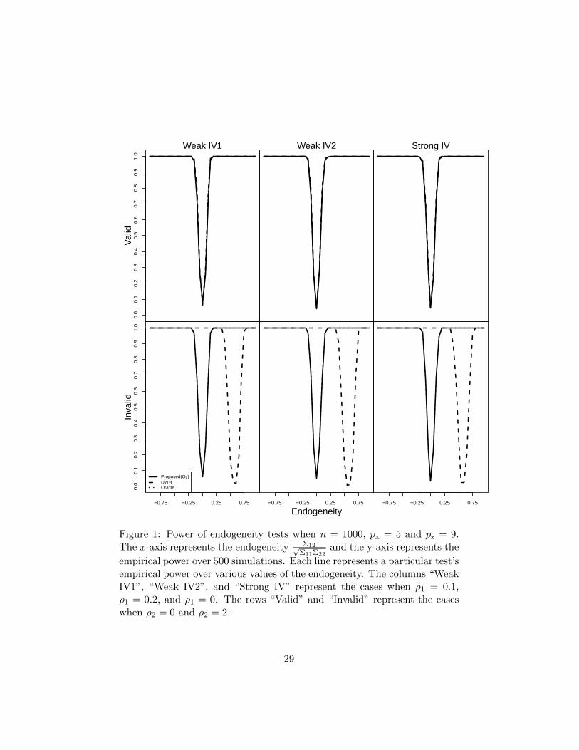
We present the result for nC(V) = 25, which is representative of the resultsfrom the simulation study; for reference, all the results of the simulationstudy are in Section ?? of the supplementary materials. First, Figure 1 con-siders the power of three comparators, the proposed testing procedure QE ,the regular DWH test and the oracle DWH test, under the low dimensionalsetting with n = 1000, px = 9, and pz = 5. Columns “Strong”,“WeakIV1”,
26

and “WeakIV2” represent different values of ρ1, specifically ρ1 = 0, ρ1 = 0.1,and ρ1 = 0.2 respectively. Rows “Valid” and “Invalid” represent differentvalues of ρ2, specifically ρ2 = 0 where all the instruments are valid andρ2 = 2 where the 6th and 7th instruments are invalid, respectively. The x-axis represents different values of endogeneity scaled by the error variances,i.e. Σ12/
√Σ11Σ22, and the y-axis is the empirical proportion of rejecting
the null hypothesis H0 over 500 simulations and is an approximation to thetest’s power.
When all the instruments are valid (i.e. the first row of Figure 1), theempirical power curves of the proposed test, the regular DWH test andthe oracle DWH are identical. However, when some of the instruments areinvalid (i.e. the second row of Figure 1), the regular DWH test cannot controlType I error and the power curve is shifted, as expected from Theorem 1.In contrast, the power curve of our proposed test is nearly identical to thatof the oracle DWH test, which is expected based on our theoretical analysisin Theorem 3. In all cases, our test maintains Type I error control.
Second, Figure 2 considers the power of our test Q, the regular DWHtest, and the oracle DWH test in the high dimensional setting with n =300, px = 150, and pz = 100. Again, when all the instruments are valid (i.e.the first row of Figure 2), all the three tests have proper size. However,as suggested by Theorem 2, the regular DWH test suffers from low powercompared to our test Q. When some instruments are invalid in the highdimensional setting (i.e. the second row of Figure 2), the DWH test cannotcontrols Type I error while our proposed test not only control Type I error,but also has power that is close to the oracle DWH test which knows a prioriwhich instruments are valid.
All the simulation results indicate that our endogeneity test controlsType I error and is a much better alternative to the regular DWH test inthe presence of invalid instruments and high dimensional covariates. In thelow dimensional setting, the power of our endogeneity test is identical tothe power of the oracle DWH test while in the high dimensional setting,our endogeneity test has better power than the regular DWH test and hasnear-optimal performance with respect to the oracle.
Finally, we provide a brief summary of the simulation results reportedin the supplementary materials, especially those concerning the violation ofregularity assumptions (IN2) and (IN3); see Section ?? of the supplementarymaterials for details. First, in Figures ?? - ?? of the supplementary mate-rials, our proposed testing procedure performs similarly to Figures 1 and 2for different individual IV strengths (represented by different values of ρ1),reiterating our comment in Section 5.3 that the proposed estimator is not
27

sensitive to the individual instrument strength assumption (IN2) requiredin the theoretical analysis. However, as discussed in Section 5.3, in highdimensions, if the instruments are weakly invalid and consequently, violate(IN3), our procedure tends to suffer. In particular, in Figures ?? and ?? ofthe supplementary materials, when the invalid IVs weakly violated exogene-ity with ρ2 = 1, our test’s size exceeds α, although at most by 5% ∼ 10%.But the power curve of the proposed test is still much better than that ofDWH test assuming valid IVs after conditioning, which tends to be shiftedaway from the null value Σ12 = 0.
7 Conclusion
In this paper, we showed that the DWH test can be highly misleading withrespect to Type I error in the presence of invalid instruments and haverelatively low power in high dimensional settings. We propose an improvedendogeneity test to remedy these failures of the DWH test and we show thatour test has proper Type I error control in the presence of invalid IVs andhas much better power than the DWH test in high dimensional settings.
References
J. Durbin. Errors in variables. Review of the International Statistical Insti-tute, 22:23–32, 1954.
D. M. Wu. Alternative tests of independence between stochastic regressorsand disturbances. Econometrica, 41:733–750, 1973.
J. Hausman. Specification tests in econometrics. Econometrica, 41:1251–1271, 1978.
R. Davidson and J. G. MacKinnon. Estimation and Inference in Economet-rics. Oxford University Press, New York, 1993.
Paul W. Holland. Causal inference, path analysis, and recursive structuralequations models. Sociological Methodology, 18(1):449–484, 1988.
Guido W Imbens and Joshua D Angrist. Identification and estimation oflocal average treatment effects. Econometrica, 62(2):467–475, 1994.
Joshua D. Angrist, Guido W. Imbens, and Donald B. Rubin. Identificationof causal effects using instrumental variables. Journal of the AmericanStatistical Association, 91(434):444–455, 1996.
28
pow
er.P
ropo
sed
Weak IV10.
00.
10.
20.
30.
40.
50.
60.
70.
80.
91.
0V
alid
Endogeneity
pow
er.P
ropo
sed
0.0
0.1
0.2
0.3
0.4
0.5
0.6
0.7
0.8
0.9
1.0
−0.75 −0.25 0.25 0.75
Inva
lid
Proposed(QE)DWHOracle
pow
er.P
ropo
sed
Weak IV2
Endogeneity
pow
er.P
ropo
sed
−0.75 −0.25 0.25 0.75
Endogeneity
pow
er.P
ropo
sed
Strong IV
Endogeneity
pow
er.P
ropo
sed
−0.75 −0.25 0.25 0.75
Figure 1: Power of endogeneity tests when n = 1000, px = 5 and pz = 9.The x-axis represents the endogeneity Σ12√
Σ11Σ22and the y-axis represents the
empirical power over 500 simulations. Each line represents a particular test’sempirical power over various values of the endogeneity. The columns “WeakIV1”, “Weak IV2”, and “Strong IV” represent the cases when ρ1 = 0.1,ρ1 = 0.2, and ρ1 = 0. The rows “Valid” and “Invalid” represent the caseswhen ρ2 = 0 and ρ2 = 2.
29

PO
WE
R.m
atrix
.pro
pose
d[ro
w.in
dex,
]
Weak IV10.
00.
10.
20.
30.
40.
50.
60.
70.
80.
91.
0V
alid
Endogeneity
PO
WE
R.m
atrix
.pro
pose
d[ro
w.in
dex,
]
Proposed(Q)DWHOracle0.
00.
10.
20.
30.
40.
50.
60.
70.
80.
91.
0
−0.75 −0.25 0.25 0.75
Inva
lid
PO
WE
R.m
atrix
.pro
pose
d[ro
w.in
dex,
]
Weak IV2
Endogeneity
PO
WE
R.m
atrix
.pro
pose
d[ro
w.in
dex,
]
−0.75 −0.25 0.25 0.75
Endogeneity
PO
WE
R.m
atrix
.pro
pose
d[ro
w.in
dex,
]
Strong IV
Endogeneity
PO
WE
R.m
atrix
.pro
pose
d[ro
w.in
dex,
]
−0.75 −0.25 0.25 0.75
Figure 2: Power of endogeneity tests when n = 300, px = 150 and pz = 100.The x-axis represents the endogeneity Σ12√
Σ11Σ22and the y-axis represents the
empirical power over 500 simulations. Each line represents a particular test’sempirical power over various values of the endogeneity. The columns “WeakIV1”, “Weak IV2”, and “Strong IV” represent the cases when ρ1 = 0.1,ρ1 = 0.2, and ρ1 = 0. The rows “Valid” and “Invalid” represent the caseswhen ρ2 = 0 and ρ2 = 2.
30

Michael P. Murray. Avoiding invalid instruments and coping with weakinstruments. The Journal of Economic Perspectives, 20(4):111–132, 2006.
Douglas Staiger and James H. Stock. Instrumental variables regression withweak instruments. Econometrica, 65(3):557–586, 1997.
Timothy G Conley, Christian B Hansen, and Peter E Rossi. Plausibly ex-ogenous. Review of Economics and Statistics, 94(1):260–272, 2012.
Miguel A. Hernan and James M. Robins. Instruments for causal inference:An epidemiologist’s dream? Epidemiology, 17(4):360–372, 2006.
Michael Baiocchi, Jing Cheng, and Dylan S. Small. Instrumental variablemethods for causal inference. Statistics in Medicine, 33(13):2297–2340,2014.
Eric Gautier and Alexandre B. Tsybakov. High-dimensional instrumentalvariables regression and confidence sets. arXiv preprint arXiv:1105.2454,2011.
A. Belloni, D. Chen, V. Chernozhukov, and C. Hansen. Sparse models andmethods for optimal instruments with an application to eminent domain.Econometrica, 80(6):2369–2429, 2012.
Victor Chernozhukov, Christian Hansen, and Martin Spindler. Post-selection and post-regularization inference in linear models with manycontrols and instruments. The American Economic Review, 105(5):486–490, 2015.
C. R. Nelson and R. Startz. Some further results on the exact sampleproperties of the instrumental variables estimator. Econometrica, 58:967–976, 1990.
Paul A Bekker. Alternative approximations to the distributions of instru-mental variable estimators. Econometrica: Journal of the EconometricSociety, pages 657–681, 1994.
John Bound, David A. Jaeger, and Regina M. Baker. Problems with instru-mental variables estimation when the correlation between the instrumentsand the endogeneous explanatory variable is weak. Journal of the Amer-ican Statistical Association, 90(430):443–450, 1995.
Jean-Marie Dufour. Some impossibility theorems in econometrics with ap-plications to structural and dynamic models. Econometrica, pages 1365–1387, 1997.
31

Eric Zivot, Richard Startz, and Charles R Nelson. Valid confidence intervalsand inference in the presence of weak instruments. International EconomicReview, pages 1119–1144, 1998.
J. Wang and E. Zivot. Inference on structural parameters in instrumentalvariables regression with weak instruments. Econometrica, 66(6):1389–1404, 1998.
Frank Kleibergen. Pivotal statistics for testing structural parameters ininstrumental variables regression. Econometrica, 70(5):1781–1803, 2002.
Marcelo J. Moreira. A conditional likelihood ratio test for structural models.Econometrica, 71(4):1027–1048, 2003.
John C. Chao and Norman R. Swanson. Consistent estimation with a largenumber of weak instruments. Econometrica, 73(5):1673–1692, 2005.
Donald W. K. Andrews, Marcelo J. Moreira, and James H. Stock. Perfor-mance of conditional wald tests in IV regression with weak instruments.Journal of Econometrics, 139(1):116–132, 2007.
Alice Nakamura and Masao Nakamura. On the relationships among severalspecification error tests presented by durbin, wu, and hausman. Econo-metrica: journal of the Econometric Society, pages 1583–1588, 1981.
Firmin Doko Tchatoka. On bootstrap validity for specification tests withweak instruments. The Econometrics Journal, 18(1):137–146, 2015.
Jinyong Hahn and Jerry Hausman. A new specification test for the validityof instrumental variables. Econometrica, 70(1):163–189, 2002.
John C Chao, Jerry A Hausman, Whitney K Newey, Norman R Swanson,and Tiemen Woutersen. Testing overidentifying restrictions with manyinstruments and heteroskedasticity. Journal of Econometrics, 178:15–21,2014.
Alexandre Belloni, Victor Chernozhukov, and Christian Hansen. Infer-ence for high-dimensional sparse econometric models. arXiv preprintarXiv:1201.0220, 2011a.
Alexandre Belloni, Victor Chernozhukov, Ivan Fernandez-Val, and ChrisHansen. Program evaluation with high-dimensional data. arXiv preprintarXiv:1311.2645, 2013.
32

Jianqing Fan and Yuan Liao. Endogeneity in high dimensions. Annals ofstatistics, 42(3):872, 2014.
Victor Chernozhukov, Christian Hansen, and Martin Spindler. Valid post-selection and post-regularization inference: An elementary, general ap-proach. 2014.
Franklin M. Fisher. The relative sensitivity to specification error of differentk-class estimators. Journal of the American Statistical Association, 61:345–356, 1966.
Franklin M. Fisher. Approximate specification and the choice of a k-classestimator. Journal of the American Statistical Association, 62:1265–1276,1967.
Whitney K. Newey. Generalized method of moments specification testing.Journal of Econometrics, 29(3):229 – 256, 1985.
Jinyong Hahn and Jerry Hausman. Estimation with valid and invalid in-struments. Annales d’conomie et de Statistique, 79/80:25–57, 2005.
Patrik Guggenberger. On the asymptotic size distortion of tests when in-struments locally violate the exogeneity assumption. Econometric Theory,28(2):387–421, 2012.
Daniel Berkowitz, Mehmet Caner, and Ying Fang. The validity of instru-ments revisited. Journal of Econometrics, 166(2):255–266, 2012.
Mehmet Caner. Near exogeneity and weak identification in generalizedempirical likelihood estimators: Many moment asymptotics. Journal ofEconometrics, 182(2):247 – 268, 2014.
Donald W. K. Andrews. Consistent moment selection procedures for gen-eralized method of moments estimation. Econometrica, 67(3):543–563,1999.
Donald WK Andrews and Biao Lu. Consistent model and moment selectionprocedures for gmm estimation with application to dynamic panel datamodels. Journal of Econometrics, 101(1):123–164, 2001.
Dylan S. Small. Sensitivity analysis for instrumental variables regressionwith overidentifying restrictions. Journal of the American Statistical As-sociation, 102(479):1049–1058, 2007.
33

Zhipeng Liao. Adaptive gmm shrinkage estimation with consistent momentselection. Econometric Theory, 29(05):857–904, 2013.
Xu Cheng and Zhipeng Liao. Select the valid and relevant moments: Aninformation-based lasso for gmm with many moments. Journal of Econo-metrics, 186(2):443–464, 2015.
Hyunseung Kang, Anru Zhang, T Tony Cai, and Dylan S Small. Instrumen-tal variables estimation with some invalid instruments and its applicationto mendelian randomization. Journal of the American Statistical Associ-ation, 111:132–144, 2016.
Michal Kolesar, Raj Chetty, John N. Friedman, Edward L. Glaeser, andGuido W. Imbens. Identification and inference with many invalid instru-ments. Journal of Business & Economic Statistics, 33(4):474–484, 2015.
Trevor Breusch, Hailong Qian, Peter Schmidt, and Donald Wyhowski. Re-dundancy of moment conditions. Journal of Econometrics, 91(1):89 – 111,1999.
Alastair Hall and Fernanda P. M. Peixe. A consistent method for the selec-tion of relevant instruments. Econometric Reviews, 22(3):269–287, 2003.
Zijian Guo, Hyunseung Kang, T Tony Cai, and S Dylan Small. Confidenceinterval for causal effects with possibly invalid instruments even after con-trolling for many confounders. 2016.
Roberto S Mariano. Approximations to the distribution functions of theil’sk-class estimators. Econometrica: Journal of the Econometric Society,pages 715–721, 1973.
James H Stock and Jonathan H Wright. Gmm with weak identification.Econometrica, pages 1055–1096, 2000.
Jeffrey M. Wooldridge. Econometric Analysis of Cross Section and PanelData. MIT press, 2nd ed. edition, 2010.
Robert Tibshirani. Regression shrinkage and selection via the lasso. Journalof the Royal Statistical Society, Series B, 58(1):267–288, 1996.
Cun-Hui Zhang and Stephanie S Zhang. Confidence intervals for low di-mensional parameters in high dimensional linear models. Journal of theRoyal Statistical Society: Series B (Statistical Methodology), 76(1):217–242, 2014.
34

Adel Javanmard and Andrea Montanari. Confidence intervals and hypothe-sis testing for high-dimensional regression. The Journal of Machine Learn-ing Research, 15(1):2869–2909, 2014.
Sara van de Geer, Peter Buhlmann, Yaacov Ritov, and Ruben Dezeure. Onasymptotically optimal confidence regions and tests for high-dimensionalmodels. The Annals of Statistics, 42(3):1166–1202, 2014.
T Tony Cai and Zijian Guo. Confidence intervals for high-dimensional linearregression: Minimax rates and adaptivity. The Annals of statistics, Toappear, 2016.
Alexandre Belloni, Victor Chernozhukov, and Lie Wang. Square-root lasso:pivotal recovery of sparse signals via conic programming. Biometrika, 98(4):791–806, 2011b.
Tingni Sun and Cun-Hui Zhang. Scaled sparse linear regression. Biometrika,101(2):269–284, 2012.
Zhao Ren, Tingni Sun, Cun-Hui Zhang, and Harrison H Zhou. Asymptoticnormality and optimalities in estimation of large gaussian graphical model.arXiv preprint arXiv:1309.6024, 2013.
Chirok Han. Detecting invalid instruments using l 1-gmm. Economics Let-ters, 101(3):285–287, 2008.
Jianqing Fan and Runze Li. Variable selection via nonconcave penalizedlikelihood and its oracle properties. Journal of the American statisticalAssociation, 96(456):1348–1360, 2001.
Peng Zhao and Bin Yu. On model selection consistency of lasso. Journal ofMachine Learning Research, 7(Nov):2541–2563, 2006.
Martin Wainwright. Information-theoretic bounds on sparsity recovery inthe high-dimensional and noisy setting. In 2007 IEEE International Sym-posium on Information Theory, pages 961–965. IEEE, 2007.
Peter Buhlmann and Sara Van De Geer. Statistics for high-dimensional data:methods, theory and applications. Springer Science & Business Media,2011.
Hannes Leeb and Benedikt M Potscher. Model selection and inference: Factsand fiction. Econometric Theory, 21(01):21–59, 2005.
35