testing for indeterminacy: an application to u.s. monetary
TRANSCRIPT

Testing for Indeterminacy:
An Application to U.S. Monetary Policy∗
Thomas A. Lubik
Department of Economics
Johns Hopkins University†
Frank Schorfheide
Department of Economics
University of Pennsylvania‡
June, 2003
JEL CLASSIFICATION: C11, C52, C62, E52
KEY WORDS: Econometric Evaluation and Testing, Rational
Expectations Models, Indeterminacy, Monetary
DSGE Models
∗We would like to thank Luca Benati, Ben Bernanke, Marco Del Negro, Roger Farmer, Peter
Ireland, Jinill Kim, Eric Leeper, Athanasios Orphanides, four anonymous referees, and seminar par-
ticipants at the Canadian Econometrics Study Group Meeting in Quebec City, the Federal Reserve
Bank of St. Louis, Johns Hopkins University, the Meetings of the Society for Computational Eco-
nomics in Aix-en-Provence, the 2002 NBER Summer Institute, the North American Econometric
Society Summer Meeting in Los Angeles, UCLA, University of Maryland, University of Pennsylva-
nia, and Tilburg University for insightful comments and suggestions. The second author gratefully
acknowledges financial support from the University Research Foundation of the University of Penn-
sylvania.†Mergenthaler Hall, 3400 N. Charles Street, Baltimore, MD 21218. Tel.: (410) 516-5564. Fax:
(410) 516-7600. Email: [email protected]‡McNeil Building, 3718 Locust Walk, Philadelphia, PA 19104. Tel.: (215) 898-8486. Fax: (215)
573-2057. Email: [email protected]

Testing for Indeterminacy:
An Application to U.S. Monetary Policy
Abstract
This paper considers a prototypical monetary business cycle model for the
U.S. economy, in which the equilibrium is undetermined if monetary policy is
‘passive’. In previous multivariate studies it has been common practice to re-
strict parameter estimates to values for which the equilibrium is unique. We
show how the likelihood-based estimation of dynamic stochastic general equilib-
rium models can be extended to allow for indeterminacies and sunspot fluctu-
ations. We construct posterior weights for the determinacy and indeterminacy
region of the parameter space and posterior estimates for the propagation of
fundamental and sunspot shocks. According to the estimated New Keynesian
model the monetary policy post 1982 is consistent with determinacy, whereas
the pre-Volcker policy is not. We find that before 1979 indeterminacy substan-
tially altered the propagation of monetary policy, demand, and supply shocks.

1
1 Introduction
Economists are increasingly making use of dynamic stochastic general equilibrium
(DSGE) models for macroeconomic analysis. In order to solve these models and
keep them tractable, linear rational expectations (LRE) models are typically used
as local approximations. However, it is well known that LRE models can have
multiple equilibria, which is often referred to as indeterminacy. Broadly speaking,
indeterminacy has two consequences. First, the propagation of fundamental shocks,
such as technology or monetary policy shocks, through the system is not uniquely
determined. Second, sunspot shocks can influence equilibrium allocations and induce
business cycle fluctuations that would not be present under determinacy.
In the popular prototypical New Keynesian monetary DSGE model (see, for in-
stance, King (2000), and Woodford (2003)) indeterminacy can arise if the monetary
policy authority follows an interest rate rule and does not raise the nominal interest
rate aggressively enough in response to an increase in inflation. While in the pres-
ence of market imperfections some sunspot fluctuations could be welfare improving
(Christiano and Harrison, 1999) others will lead to a substantial deterioration of
welfare. Hence, a central bank that is concerned about the least favorable outcome
has a strong incentive to choose a policy that leads to determinacy.
It has been suggested by Clarida, Galı, and Gertler (2000), henceforth CGG,
that the U.S. monetary policy before 1979 viewed through the lens of a standard
New Keynesian DSGE model was inconsistent with equilibrium determinacy. Self-
fulfilling expectations are potentially one of the explanations for the high inflation
episode in the 1970s. Beginning with Paul Volcker’s tenure as Board Chairman
and, later on, Alan Greenspan’s the Federal Reserve implemented a much more
aggressive rule that suppresses self-fulfilling beliefs. Studying indeterminacy can
therefore contribute to our understanding of the macroeconomic instability during
the 1970s and further the design of beneficial policy rules.
The first contribution of this paper is to provide econometric tools that allow for
a systematic assessment of the quantitative importance of equilibrium indeterminacy

2
and the propagation of fundamental and sunspot shocks in the context of a DSGE
model. While it is well known how to construct a likelihood function of a DSGE
model for the determinacy region of the parameter space, we show how the likelihood
function can be extended to the indeterminacy region. Based on results obtained
in Lubik and Schorfheide (2003) we index the multiple solutions that arise under
indeterminacy through additional parameters that characterize the transmission of
fundamental shocks and the distribution of sunspot shocks. We discuss the extent
to which these additional and the original DSGE model parameters are identifiable
and illustrate that even if the structural parameters are only partially identified the
likelihood function provides interesting and useful information about indeterminacy
and the propagation of shocks.
To summarize the information contained in the likelihood function we use a
Bayesian approach. The likelihood function is combined with a prior density for the
model parameters and the resulting function is interpreted as posterior density of the
parameters given the data. In the directions of the parameter space in which there
is no identification, that is, where the likelihood function is flat, the prior density
is not updated. Nevertheless, the posterior density provides a coherent summary of
prior and sample information. The Bayesian approach lets us calculate probability
weights for the determinacy and indeterminacy region of the parameter space and
posterior distributions for the propagation of shocks in the model.
The second contribution of this paper is an application of our econometric tools
to a New Keynesian business cycle model. We revisit the question whether U.S.
monetary policy was stabilizing pre- and post-Volcker. Our estimates confirm the
finding of CGG that U.S. monetary policy before 1979 has contributed to aggregate
instability and that policy has become markedly more stabilizing during the Volcker-
Greenspan period.
Our multivariate analysis has several advantages over the univariate approach
pursued by CGG. First and foremost, we are able to estimate the additional pa-
rameters that characterize the model solution under indeterminacy and can assess
the importance of sunspots and the propagation of structural shocks. We offer two

3
interpretations of the pre-Volcker dynamics of output, inflation, and interest rates
in the U.S.. Under the first interpretation the presence of indeterminacy changed
the propagation of the monetary policy, demand, and supply shocks, but sunspot
shocks played no role. Under the second interpretation, the responses to fundamen-
tal shocks resemble the determinacy responses. Additional sunspot shocks caused
substantial inflation and interest rate fluctuations but had only a small effect on
aggregate output. The data slightly favor the first interpretation.
More generally, indeterminacy is a property of a dynamic system and should
therefore studied through multivariate analysis. In most models the indeterminacy
region is a complicated function of several parameters, not just the parameters of a
monetary policy reaction function. In the context of DSGE models full-information
estimators are typically more efficient than instrumental variable estimators based
on single equations. Ruge-Murcia (2002) provides some simulation evidence. How-
ever, the potential presence of sunspot fluctuations may cause identification prob-
lems that are not readily transparent in a univariate analysis. We provide an ex-
ample in which the parameter that marks the determinacy region of the parameter
space is only identifiable under indeterminacy. Nevertheless, it is possible to infer
whether data have been generated from the determinacy region.
A weakness of our approach is that it is potentially sensitive to model misspec-
ification. The endogenous dynamics in the indeterminacy region of the parameter
space are richer than in the determinacy region. Thus, propagation mechanisms
omitted from the specification of the DSGE model tend to bias our posteriors toward
indeterminacy. However, this weakness is shared by all system-based approaches to
evaluation of indeterminacies. To check the robustness of our empirical findings we
compare the pre-Volcker fit of the simple New Keynesian model to a richer model
specification with habit formation and backward-looking price setters which we re-
strict to the determinacy region. We find that the data favor the indeterminacy
interpretation provided by the simple model.
It has also been noted in the literature that the association of passive monetary
policy with indeterminacy is very model specific. For instance, Dupor (2001) shows

4
that in a continuous time model with endogenous investment passive monetary pol-
icy can be consistent with determinacy. Hence our empirical finding that prior to
1979 aggregate fluctuations of output, inflation, and interest rates are best described
by indeterminacy is conditional on the model choice. However, since the New Key-
nesian monetary model considered in this paper has become a standard benchmark
in the literature, we regard it as a good starting point for the application of our
techniques.
Other empirical studies of indeterminacy fall broadly into two categories: First,
calibration exercises, such as Farmer and Guo (1994), Perli (1998) or Schmitt-
Grohe (1997, 2000), that attempt to quantify the extent to which sunspot shocks
are helpful in matching model properties to business cycle facts. They face the
common difficulty of specifying the stochastic properties of the sunspot shock. The
typical practice is to choose its variance to match the observed variance of out-
put. While these authors demonstrate the qualitative importance of indeterminacy,
their quantitative conclusions are more tenuous. As we show in this paper, equilib-
rium indeterminacy does not imply that aggregate fluctuations are in fact driven by
sunspots.
An alternative empirical approach is taken by Farmer and Guo (1995) and Salyer
and Sheffrin (1998). They try to identify sunspot shocks from rational expecta-
tions residuals that are left unexplained by exogenous fundamentals. Although
this approach imposes more structure than simple calibration, it cannot distinguish
between omitted fundamentals and actual sunspots. All of the cited papers ask
the question ‘can the observed business cycle fluctuations be explained by sunspot
shocks?’ Our approach treats the determinacy and indeterminacy hypotheses sym-
metrically and quantifies the empirical evidence in favor of one against the other.
The closest theoretical and empirical precursors1 to this paper are Leeper and
Sims (1994), Kim (2000), Ireland (2001), and Rabanal and Rubio-Ramirez (2002)
1In a much earlier contribution Jovanovic (1989) provides a general characterization of the identi-
fication problems inherent in econometric analyses of models with multiple equilibria. Cooper (2001)
surveys different empirical approaches to equilibrium indeterminacy from several fields.
5
who estimate monetary models similar to ours with likelihood-based techniques.
Ireland (2001) finds significant evidence of a change in monetary policy behavior
after 1979. However, all of the above authors explicitly rule out indeterminate
equilibria in their estimation strategy. If the data are in fact best described by
parameters from the indeterminacy region, a restriction of the estimates to the
determinacy region will result in biased parameter estimates. This problem vanishes
if the model is estimated over the entire parameter space.
The paper is structured as follows. In Section 2 we present the log-linearized
New Keynesian monetary business cycle model to which our econometric tools are
applied. Section 3 illustrates the econometric tools in the context of a very sim-
ple one-equation model. The representation of the indeterminacy solutions for a
canonical LRE model is presented in Section 4. Section 5 discusses some of the
advantages of our inferential approach. Empirical results for the New Keynesian
model are presented in Section 6. Section 7 concludes and the Appendix provides
computational details.
2 A Model for the Analysis of Monetary Policy
For the empirical analysis presented in this paper we consider a prototypical New
Keynesian monetary DSGE model. This model can be summarized by the following
three equations:
xt = IEt[xt+1]− τ(Rt − IEt[πt+1]) + gt, (1)
πt = βIEt[πt+1] + κ(xt − zt), (2)
Rt = ρRt−1 + (1− ρ) (ψ1πt + ψ2[xt − zt]) + εR,t, (3)
where x is output, π is inflation, and R the nominal interest rate. The tilde denotes
percentage deviations from a steady state or, in the case of output, from a trend
path. Using log-linear approximations these equations can be derived from a micro-
founded dynamic general equilibrium model. Details can be found, for instance, in
King (2000) and Woodford (2003).

6
Equation (1) is an intertemporal Euler equation obtained from the households’
optimal choice of consumption and bond holdings. Since the underlying model has
no investment, output is proportional to consumption up to an exogenous process
that can be interpreted as time-varying government spending or, more broadly, as
preference change. The net effects of these exogenous shifts on the Euler equation
are captured in the process gt. The parameter 0 < β < 1 is the households’ discount
factor and τ > 0 can be interpreted as intertemporal substitution elasticity.
The production sector in the underlying model economy is characterized by
a continuum of monopolistically competitive firms, each of which faces a down-
ward sloping demand curve for its differentiated product. Prices are sticky due to
quadratic adjustment costs in nominal prices or a Calvo-style rigidity that allows
only a fraction of firms to adjust their prices. The resulting inflation dynamics
are described by the expectational Phillips curve (2) with slope κ. The process zt
captures exogenous shifts of the marginal costs of production.
The third equation describes the behavior of the monetary authority. The central
bank follows a nominal interest rate rule by adjusting its instrument to deviations of
inflation and output from their respective target levels. The shock εR,t can be inter-
preted as unanticipated deviation from the policy rule or as policy implementation
error. Its standard deviation is denoted by σR.
We assume that both gt and zt evolve according to univariate AR(1) processes
with coefficients ρg and ρz, respectively:
gt = ρggt−1 + εg,t, zt = ρzzt−1 + εz,t. (4)
We allow for non-zero correlation ρgz between the innovations εg,t and εz,t and denote
their standard deviations by σg and σz. The parameters of the log-linearized DSGE
model are collected in the vector
θ = [ψ1, ψ2, ρR, κ, τ, ρg, ρz, ρgz, σR, σg, σz]
with domain Θ. The linear rational expectations model comprised of Equations (1)
to (4) can be rewritten in the canonical form
Γ0(θ)st = Γ1(θ)st−1 +Ψ(θ)εt +Π(θ)ηt, (5)

7
where
st = [xt, πt, Rt, IEt[xt+1], IEt[πt+1], gt, zt]′
εt = [εR,t, εg,t, εz,t]′
ηt = [(xt − IEt−1[xt]), (πt − IEt−1[πt])]′.
In our model the dimension of st is n = 7. There are l = 3 fundamental shocks
and the vector of rational expectations forecast errors, ηt, has dimension k = 2. We
assume that in addition to the fundamental shock εt the agents observe an exogenous
sunspot shock ζt.
It is well known in the literature that this log-linear model can give rise to self-
fulfilling expectations if the central bank does not raise the nominal interest rate
aggressively enough in response to inflation. In this case not just the fundamental
shocks εt but also the sunspot shock ζt can influence the dynamics of output, infla-
tion, and interest rates. More formally, since the model (5) is linear and the only
sources of uncertainty are the shocks εt and ζt the forecast errors for output and
inflation can be expressed as as
ηt = A1εt +A2ζt (6)
where A1 is k× l and A2 is k× 1. Solution algorithms for LRE systems construct a
mapping from the shocks to the expectation errors either implicitly, e.g., Blanchard
and Kahn (1980), or explicitly, e.g., Sims (2002).
Since the transversality conditions of the underlying optimization problems im-
pose restrictions on the growth rates of st, it is common to consider only solutions
to the LRE system for which st is non-explosive. Three cases can be distinguished:
(i) non-existence of a stable solution, (ii) existence of a unique stable solution (de-
terminacy) in which A1 is determined by the structural parameters θ and A2 = 0,
and (iii) existence of multiple stable solutions (indeterminacy) in which A1 is not
uniquely determined by θ and A2 can be non-zero. Loosely speaking, the mone-
tary DSGE model described by Equations (1) to (3) has a unique stable solution if
the central bank raises the real interest rate in response to inflation (ψ1 > 1) and
8
has multiple stable solutions otherwise. The former policy is often called ‘active’,
whereas the latter is regarded as ‘passive’.
In the existing literature system-based econometric inference has been limited
to the subset of the parameter space for which the stable solution is unique. The
novelty of this paper is to extend estimation and inference to the indeterminacy
region of the parameter space. In particular we want to be able to assess the evidence
of determinacy versus indeterminacy and estimate the propagation of fundamental
and sunspot shocks under indeterminacy.
3 Econometric Inference
In order to extend the estimation of LRE models to the indeterminacy region of the
parameter space we have to overcome two challenges. First, we need a convenient
representation for the multiplicity of solutions. Here we build upon results that
we have derived in Lubik and Schorfheide (2003). Second, we have to pay careful
attention to identification issues. Some of the identification problems are trivial. For
instance, under determinacy the variance of the sunspot shock ζt is not identifiable
since A2 = 0 and the sunspot shock has no influence on the endogenous variables.
Other identification problems are less transparent. For example, in some instances
one of the model parameters marks the determinacy region, but is only identifiable
under indeterminacy. Nevertheless, it is typically possible to learn from the data
whether they have been generated under determinacy or indeterminacy. We discuss
these challenges and our solution in the context of the following single equation
model
yt =1
θIEt[yt+1] + εt, (7)
where εt ∼ iid(0, 1) and θ ∈ Θ = [0, 2]. This model can be cast in the canonical
form (5) by introducing the conditional expectation ξt = IEt[yt+1] and the forecast
error ηt = yt − ξt−1. Thus,
ξt = θξt−1 − θεt + θηt. (8)
9
We chose this very simple example in order to make the properties of our econometric
approach transparent. Extensions to the monetary DSGE model of Section 2 will
be discussed in Sections 4 and 5.
The stability properties of the difference equation (8) hinge on the value of the
parameter θ. If θ > 1 (determinacy) the only stable solution2 is of the form ξt = 0,
which obtains if ηt = εt and
yt = εt (9)
Thus, for θ > 1 the endogenous variable follows an iid process. Its stochastic
properties do not depend on the value of θ. We denote the determinacy region of
the parameter space by ΘD = (1, 2].
If θ ≤ 1 (indeterminacy) the stability requirement imposes no restrictions on
the rational expectations forecast error ηt:
ηt = Mεt + ζt (10)
Here M is a parameter, unrelated to θ, that arises because the effect of the fun-
damental shock εt is not determined. Moreover, part of the forecast error may be
due to a sunspot shock ζt that is unrelated to the fundamental disturbance εt. For
simplicity we assume in this section that ζt = 0 for all t. Replacing IEt[yt+1] in (7)
by yt+1− Mεt+1 leads to an ARMA(1,1) representation for yt that depends on both
θ and M :
yt − θyt−1 = Mεt + θεt−1. (11)
While yt is generally serially correlated under indeterminacy, it reduces to the iid
process yt = εt that is invariant to θ in the special case of M = 1. If the lagged
variables yt−1 and εt−1 are regarded as ‘states’, then the M = 1 solution can be inter-
preted as minimal-state-variable (MSV) solution in the spirit of McCallum (1983).
For the remainder of this section we will center the indeterminacy solutions around
M = 1 and use the reparameterization M = 1 +M . The indeterminacy region of
the parameter space is labelled ΘI = [0, 1].
2We regard the random walk case of θ = 1 as ‘stable’ in this example.

10
The goal of the econometric analysis is to summarize the sample information
about θ and M . More specifically, we are interested in assessing the hypothesis
θ ∈ ΘD versus θ ∈ ΘI , and estimate the propagation of the shock εt, which under
indeterminacy depends on both θ and M . Our inference is, of course, constrained
by the restricted identifiability of the model parameters.
Let us consider the likelihood function for a sample of observations Y T =
[y1, . . . , yT ]′. The likelihood L(θ,M |Y T ) is the joint probability density function of
Y T given the parameters. We will assume that εt is normally distributed and split
the likelihood function into two parts which correspond to the determinacy and the
indeterminacy region of the parameter space, respectively. Let f(x) = x < a be
the indicator function that is one if x < a and zero otherwise. Then
L(θ,M |Y T ) = θ ∈ ΘILI(θ,M |YT ) + Θ ∈ ΘDLD(Y
T ), (12)
where
LD(YT ) = (2π)−T/2 exp
−1
2Y ′TYT
LI(θ,M |YT ) = (2π)−T/2|ΓY (θ,M)|−1/2 exp
−1
2Y ′TΓ
−1Y (θ,M)YT
and ΓY (θ,M) denotes the covariance matrix of the vector Y T under the ARMA
representation (11). In the determinacy region of the parameter space the likelihood
function is invariant to θ and M , that is, LD is constant. In other words: the
parameters θ and M are not identifiable. Moreover, for M = 0 the indeterminacy
likelihood is constant as a function of θ:
LI(θ,M = 0|Y T ) = LD(YT ). (13)
To illustrate the shape of the likelihood function we generate two data sets from
the one-equation LRE model, denoted by Y T (D) and Y T (I). The sample size is
T = 30. Y T (D) is generated from the determinacy region of the parameter space
and consists of iidN (0, 1) draws, whereas Y T (I) is generated based on θ = 0.8 and
M = 1. Figure 1 depicts the surface of the log-likelihood functions (standardized by
their respective maxima) for the two samples. Although both likelihood functions
11
are flat for θ > 1 they do provide useful information. Since the autocovariances of
the iid sample Y T (D) are near zero the likelihood function is small in the region of
the parameter space where θ ≤ 1 and M is very different from zero. Lack of serial
correlation is interpreted as evidence for determinacy. The indeterminacy sample
Y T (I), on the other hand, exhibits serial correlation. Hence, the likelihood function
is high for parameter values that are consistent with the degree of serial correlation
in the sample. It also appears to be informative with respect to both θ and M .
If the goal of the econometric analysis were pure testing of determinacy versus
indeterminacy, this could in principle be achieved with a likelihood ratio test of the
form
LR =sup0≤θ≤1,M LI(θ,M |Y
T )
LD(Y T ). (14)
The sampling distribution of LR under the null hypothesis and the resulting critical
values are non-standard because the parameters θ andM are non-identifiable under
the null hypothesis. Andrews and Ploberger (1994) show that an optimal test for
this problem is of the form
LRave =
∫sup0≤θ≤1,M LI(θ,M |Y
T )
LD(Y T )w(θ,M) dθ · dM (15)
where w(θ,M) assigns large weight to alternatives against which the test is supposed
to have high power. To construct such a test statistic one has to know the directions
of the parameter space that lack identification. It is trivial in this one-equation
example, but can become prohibitively complicated in large LRE models with many
parameter restrictions.
However, rather than asking the question ‘are the data consistent with equilib-
rium determinacy’ it is more useful to construct probability weights for the determi-
nacy and indeterminacy regions of the parameter space conditional on the observed
data. These probabilities can then be used to weight the parameter estimates and
the predictions that the model delivers conditional on the two regions of the param-
eter space. Hence, we will follow a Bayesian approach by placing a prior distribution
with density p(θ,M) on the parameters θ and M and conducting inference based
on the posterior distribution of the parameters given the data Y T . This posterior
12
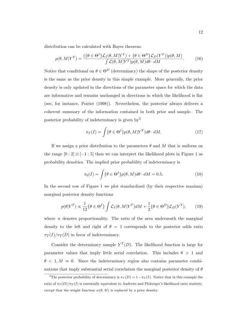
distribution can be calculated with Bayes theorem:
p(θ,M |Y T ) =(θ ∈ ΘILI(θ,M |Y
T ) + θ ∈ ΘDLD(YT ))p(θ,M)∫
L(θ,M |Y T )p(θ,M)dθ · dM. (16)
Notice that conditional on θ ∈ ΘD (determinacy) the shape of the posterior density
is the same as the prior density in this simple example. More generally, the prior
density is only updated in the directions of the parameter space for which the data
are informative and remains unchanged in directions in which the likelihood is flat
(see, for instance, Poirier (1998)). Nevertheless, the posterior always delivers a
coherent summary of the information contained in both prior and sample. The
posterior probability of indeterminacy is given by3
πT (I) =
∫θ ∈ ΘIp(θ,M |Y T )dθ · dM. (17)
If we assign a prior distribution to the parameters θ and M that is uniform on
the range [0 : 2]⊗ [−1 : 5] then we can interpret the likelihood plots in Figure 1 as
probability densities. The implied prior probability of indeterminacy is
π0(I) =
∫θ ∈ ΘIp(θ,M)dθ · dM = 0.5. (18)
In the second row of Figure 1 we plot standardized (by their respective maxima)
marginal posterior density functions
p(θ|Y T ) ∝1
12θ ∈ ΘI
∫LI(θ,M |Y
T )dM +1
2θ ∈ ΘDLD(Y
T ), (19)
where ∝ denotes proportionality. The ratio of the area underneath the marginal
density to the left and right of θ = 1 corresponds to the posterior odds ratio
πT (I)/πT (D) in favor of indeterminacy.
Consider the determinacy sample Y T (D). The likelihood function is large for
parameter values that imply little serial correlation. This includes θ > 1 and
θ < 1,M ≈ 0. Since the indeterminacy region also contains parameter combi-
nations that imply substantial serial correlation the marginal posterior density of θ
3The posterior probability of determinacy is πT (D) = 1−πT (I). Notice that in this example the
ratio of πT (D)/πT (I) is essentially equivalent to Andrews and Ploberger’s likelihood ratio statistic,
except that the weight function w(θ,M) is replaced by a prior density.

13
is substantially lower for θ < 1 than it is for θ > 1. Thus, the posterior odds strongly
favor determinacy. Just as the likelihood ratio test of Andrews and Ploberger has
no power against the θ < 1 andM = 0 indeterminacy alternative, the Bayesian pro-
cedure will interpret a long iid sample as evidence in favor of determinacy as long
as the prior distribution for M is continuous and assigns zero probability to M = 0.
If the data exhibit serial correlation then there are values of θ < 1 and M 6= 0 for
which the likelihood function is substantially larger than in the determinacy region
which is also reflected in the marginal posterior density of θ. Even based on our
short sample the posterior probability of indeterminacy is essentially one.4
The findings of this section can be summarized as follows. In the context of
a one-equation model we have shown that an additional parameter M , which is
unrelated to θ is needed to characterize the dynamics of yt. We have discussed the
resulting identification problems and illustrated how a Bayesian approach can be
used to make inference with respect to determinacy versus indeterminacy and the
parameters that determine the law of motion for yt. In the following section we will
provide a characterization for the solutions of the canonical LRE model (5) under
indeterminacy.
4 Solution of the Canonical LRE Model
In solving the LRE system (5) we closely follow the approach of Sims (2002), ex-
tended in Lubik and Schorfheide (2003).5 To keep the exposition simple we assume
4The posterior probabilities provide a consistent test for indeterminacy. If θ ∈ ΘD then πT (I)
will converge in probability to zero as the sample size T tends to infinity. If θ ∈ ΘI then πT (I)
will converge to one. The latter convergence will fail on a subset of the parameter space, namely
θ < 1 and M = 0, which has probability zero under our prior distribution. A formal proof can
be constructed by deriving a large sample approximation of∫
LI(θ,M |Y T )p(θ,M)dθ · dM as in
Phillips (1996), Kim (1998), and Fernandez-Villaverde and Rubio-Ramirez (2001) and then applying
the argument in Hannan (1980) to treat the identification problem that arises in ‘determinacy’
samples.5Sims (2002) solution procedure generalizes the method proposed by Blanchard and Kahn (1980).
In particular, it does not require the researcher to separate the list of endogenous variables into
14
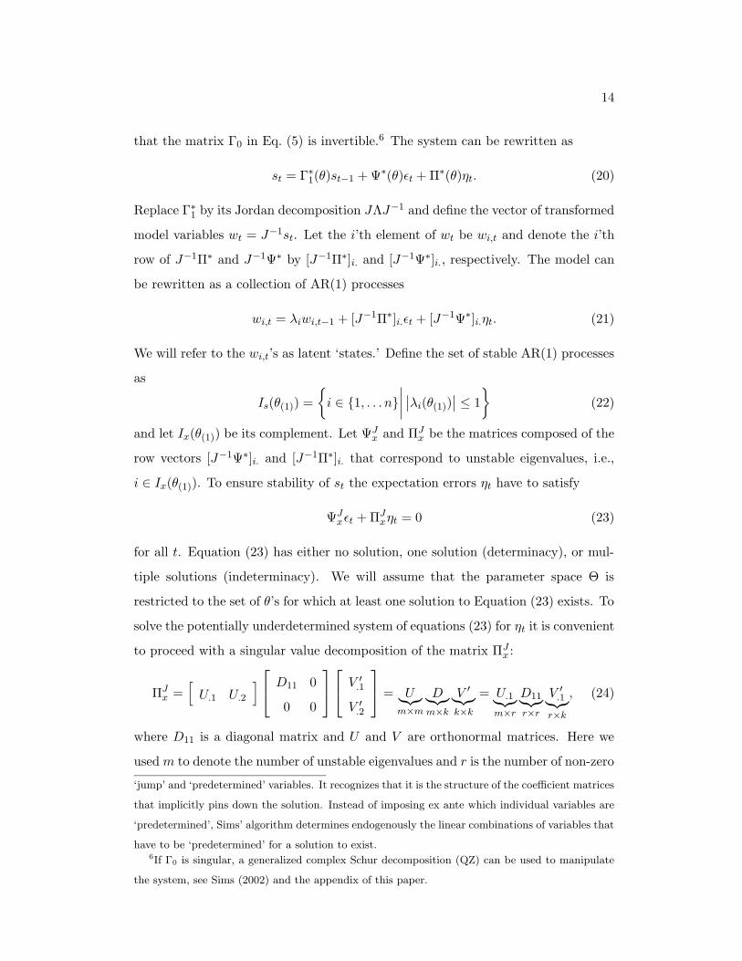
that the matrix Γ0 in Eq. (5) is invertible.6 The system can be rewritten as
st = Γ∗1(θ)st−1 +Ψ∗(θ)εt +Π∗(θ)ηt. (20)
Replace Γ∗1 by its Jordan decomposition JΛJ−1 and define the vector of transformed
model variables wt = J−1st. Let the i’th element of wt be wi,t and denote the i’th
row of J−1Π∗ and J−1Ψ∗ by [J−1Π∗]i. and [J−1Ψ∗]i., respectively. The model can
be rewritten as a collection of AR(1) processes
wi,t = λiwi,t−1 + [J−1Π∗]i.εt + [J−1Ψ∗]i.ηt. (21)
We will refer to the wi,t’s as latent ‘states.’ Define the set of stable AR(1) processes
as
Is(θ(1)) =
i ∈ 1, . . . n
∣∣∣∣∣∣λi(θ(1))
∣∣ ≤ 1
(22)
and let Ix(θ(1)) be its complement. Let ΨJx and ΠJ
x be the matrices composed of the
row vectors [J−1Ψ∗]i. and [J−1Π∗]i. that correspond to unstable eigenvalues, i.e.,
i ∈ Ix(θ(1)). To ensure stability of st the expectation errors ηt have to satisfy
ΨJxεt +ΠJ
xηt = 0 (23)
for all t. Equation (23) has either no solution, one solution (determinacy), or mul-
tiple solutions (indeterminacy). We will assume that the parameter space Θ is
restricted to the set of θ’s for which at least one solution to Equation (23) exists. To
solve the potentially underdetermined system of equations (23) for ηt it is convenient
to proceed with a singular value decomposition of the matrix ΠJx :
ΠJx =
[U.1 U.2
] D11 0
0 0
V ′.1
V ′.2
= U︸︷︷︸
m×m
D︸︷︷︸m×k
V ′︸︷︷︸k×k
= U.1︸︷︷︸m×r
D11︸︷︷︸r×r
V ′.1︸︷︷︸r×k
, (24)
where D11 is a diagonal matrix and U and V are orthonormal matrices. Here we
usedm to denote the number of unstable eigenvalues and r is the number of non-zero
‘jump’ and ‘predetermined’ variables. It recognizes that it is the structure of the coefficient matrices
that implicitly pins down the solution. Instead of imposing ex ante which individual variables are
‘predetermined’, Sims’ algorithm determines endogenously the linear combinations of variables that
have to be ‘predetermined’ for a solution to exist.6If Γ0 is singular, a generalized complex Schur decomposition (QZ) can be used to manipulate
the system, see Sims (2002) and the appendix of this paper.

15
singular values of ΠJx . Recall that k is the dimension of the vector of forecast errors ηt
and l denotes the number of exogenous shocks. Let p be the dimension of the sunspot
shock ζt. The following proposition is proved in Lubik and Schorfheide (2003):
Proposition 1 If there exists a solution to Eq. (23) that expresses the forecast
errors as function of the fundamental shocks εt and sunspot shocks ζt, it is of the
form
ηt = η1εt + η2ζt (25)
= (−V.1D−111 U
′.1Ψ
Jx + V.2M)εt + V.2Mζζt,
where M is an (k− r)× l matrix, Mζ is a (k− r)× p matrix, and the dimension of
V.2 is k × (k − r). The solution is unique if k = r and V.2 is zero.
The representation for the rational expectations forecast errors leads to the
following law of motion for st:
st = Γ∗1(θ)st−1 + [Ψ∗(θ)−Π∗(θ)V.1(θ)D−111 (θ)U
′.1(θ)Ψ
Jx(θ)]εt (26)
+Π∗(θ)V.2(θ)(Mεt +Mζζt).
Under determinacy V.2 = 0 and the terms in the second line of Equation (26) drop
out. In this case the dynamics of xt are purely a function of the parameter vector
θ. Indeterminacy introduces additional parameters and changes the nature of the
solution in two dimensions. First, the propagation of the structural shocks εt is not
uniquely determined as it depends on the matrix M . Second, the dynamics of st
are potentially affected (Mζ 6= 0) by the sunspot shocks ζt. In the monetary DSGE
model of Section 2 the degree of indeterminacy k − r is at most 1. Hence, we set
p = 1 and impose the normalizationMζ = 1. The standard deviation of the sunspot
shock, denoted by σζ , is treated as additional parameter. Since it is not possible
to identify the covariances of the sunspot shock with the fundamental shocks in
addition to M we use the normalization IE[εtζt] = 0.
In Section 3 we reparameterized the indeterminacy solutions by M = 1 +M ,
such thatM = 0 corresponded to yt = εt. While we consider all possible values of M

16
in our estimation procedure we specify a prior distribution that is centered around
one particular solution. We do this by replacing M withM∗(θ)+M and setting the
prior mean for M equal to zero. We find it desirable to choose M ∗(θ) such that the
impulse responses ∂st/∂ε′t are continuous at the boundary between the determinacy
and indeterminacy region. According to our prior mean, small changes of θ do not
lead to drastic changes in the propagation of fundamental shocks.
One candidate for M ∗(θ) is the minimal-state-variable solution considered in
Section 3. Suppose in a model with a one-dimensional indeterminacy it is possible
to identify an eigenvalue function λi∗(θ) such that |λi∗(θ)| is greater than one in
the determinacy region (θ ∈ ΘD) and less than one in the indeterminacy region
(θ ∈ ΘI). In this case a baseline solution could be constructed by solving the
system of equations
[J−1Π∗]iεt + [J−1Ψ∗]iηt = 0 (27)
for i ∈ Ix(θ) and i = i∗. This solution has the feature that it eliminates as many
‘states’ wi,t as the determinacy solution.
While it is possible to define and track eigenvalue functions in the model pre-
sented in Section 2, it is difficult in larger systems. Moreover, there is no guarantee
that this procedure yields economically plausible impulse response for values of θ
that are not in the immediate vicinity of the determinacy region. Hence, we proceed
with an alternative method. For every vector θ ∈ ΘI we construct a vector θ = g(θ)
that lies on the boundary of the determinacy region and chooseM ∗(θ) such that the
response of st to εt conditional on θ mimics the response conditional on θ. Thus,
we compare
∂st∂ε′t
(θ,M) = Ψ∗(θ)−Π∗(θ)V.1(θ)D−111 (θ)U
′.1(θ)Ψ
Jx(θ) + Π∗(θ)V.2(θ)M (28)
B1(θ) +B2(θ)M
to∂st∂ε′t
(g(θ), ·) = B1(g(θ)). (29)

17
In our application we minimize the discrepancy using a least squares criterion and
choose
M∗(θ) = [B2(θ)′B2(θ)]
−1B2(θ)′ ∗ [B1(g(θ))−B1(θ)] (30)
The function g(θ) is obtained by replacing ψ1 in the vector θ with
ψ1 = 1−βψ2
κ
(1
β− 1
), (31)
which marks the boundary between the determinacy and indeterminacy region for
the model presented in Section 2.7 We will refer to the solution M = M∗(θ) as
baseline indeterminacy solution. The impulse response analysis in Section 6 will
reveal that, by and large, the responses under the baseline indeterminacy solution
are similar to the determinacy responses, expect for the scaling of the interest rate
response which is sensitive to the choice of ψ1.
While our baseline indeterminacy solution provides a plausible benchmark, our
estimation under indeterminacy is not restricted to this specific solution. We only
use it to center our prior distribution for M in Equation (26). Based on the solution
described in this section we construct a likelihood function L(θ,M, σζ |YT ) that is
used for Bayesian inference as described in Section 3.
5 Discussion
Before proceeding with the empirical analysis we will discuss some of the virtues
and limitations of our inference approach and compare it to alternatives that have
been proposed in the literature. To focus the discussion we consider a special case
of the model presented in Section 2. Suppose that the monetary authority does
not attempt to smooth the nominal interest rate (ρR = 0) and only targets current
inflation (ψ2 = 0). Moreover, the exogenous processes gt and zt have no serial
correlation, that is, ρg = ρz = 0. Define the conditional expectations ξxt = IEt[xt+1],
7The derivation of this formula is relegated to a Technical Appendix that is available from the
authors upon request.

18
ξπt = IEt[πt+1] and the vector ξt = [ξxt , ξπt ]′. The vector ξt evolves according to
ξt =
1 + κτ
β τ(ψ1 −1β )
−κβ
1β
︸ ︷︷ ︸Γ∗1
ξt−1 +
τ −1 0
0 0 κ
︸ ︷︷ ︸Ψ∗
εt +
1 + κτ
β τ(ψ1 −1β )
−κβ
1β
︸ ︷︷ ︸Π∗
ηt.
(32)
Since the simplified model has a block-triangular structure the vector of expectation
errors ηt can be determined by applying the methods described in Section 4 to the
two-dimensional subsystem (32).
The dynamics of the system depend on the eigenvalues of Γ∗1. It can be shown
that both eigenvalues are unstable if ψ1 > 1 (see, for instance, Bullard and Mitra
(2002) or Lubik and Marzo (2003)). In this case the only stable solution is ξt = 0
which uniquely determines the forecast errors ηt = −Π∗Ψ∗εt. Tedious but straight-
forward algebraic manipulations lead to the following law of motion for output,
inflation, and interest rates:
xt
πt
Rt
=
1
1 + κτψ1
−τ 1 τκψ1
−κτ κ −κ
1 κψ1 −κψ1
εR,t
εg,t
εz,t
. (33)
The model exhibits no dynamics because the solution suppresses the two roots of the
autoregressive matrix Γ∗1. An unanticipated monetary contraction leads to a one-
period fall in output and inflation. An Euler-equation shock εg,t increases output,
inflation, and interest rate. A Phillips-curve shock εz,t raises output, but lowers
inflation and interest rates for one period.
If ψ1 < 1 only one of the eigenvalues is unstable and the evolution of the en-
dogenous variables can be described as follows:
xt
πt
Rt
=
1
1 + κτψ1
−τ 1 τκψ1 (λ2 − 1− κτψ1)
−κτ κ −κ κλ2
1 κψ1 −κψ1 ψ1κλ2
εt
ζt
(34)
+
(β(λ2 − 1)− τκ)/κ
1
ψ1
w1,t−1,
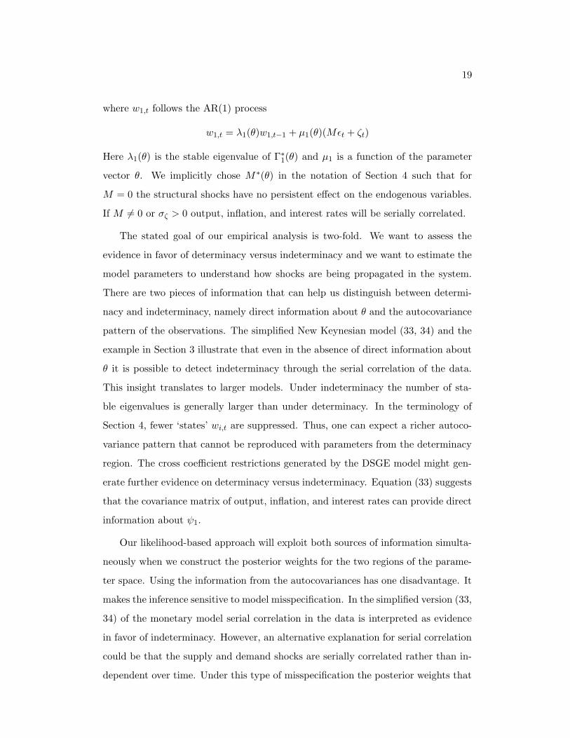
19
where w1,t follows the AR(1) process
w1,t = λ1(θ)w1,t−1 + µ1(θ)(Mεt + ζt)
Here λ1(θ) is the stable eigenvalue of Γ∗1(θ) and µ1 is a function of the parameter
vector θ. We implicitly chose M ∗(θ) in the notation of Section 4 such that for
M = 0 the structural shocks have no persistent effect on the endogenous variables.
If M 6= 0 or σζ > 0 output, inflation, and interest rates will be serially correlated.
The stated goal of our empirical analysis is two-fold. We want to assess the
evidence in favor of determinacy versus indeterminacy and we want to estimate the
model parameters to understand how shocks are being propagated in the system.
There are two pieces of information that can help us distinguish between determi-
nacy and indeterminacy, namely direct information about θ and the autocovariance
pattern of the observations. The simplified New Keynesian model (33, 34) and the
example in Section 3 illustrate that even in the absence of direct information about
θ it is possible to detect indeterminacy through the serial correlation of the data.
This insight translates to larger models. Under indeterminacy the number of sta-
ble eigenvalues is generally larger than under determinacy. In the terminology of
Section 4, fewer ‘states’ wi,t are suppressed. Thus, one can expect a richer autoco-
variance pattern that cannot be reproduced with parameters from the determinacy
region. The cross coefficient restrictions generated by the DSGE model might gen-
erate further evidence on determinacy versus indeterminacy. Equation (33) suggests
that the covariance matrix of output, inflation, and interest rates can provide direct
information about ψ1.
Our likelihood-based approach will exploit both sources of information simulta-
neously when we construct the posterior weights for the two regions of the parame-
ter space. Using the information from the autocovariances has one disadvantage. It
makes the inference sensitive to model misspecification. In the simplified version (33,
34) of the monetary model serial correlation in the data is interpreted as evidence
in favor of indeterminacy. However, an alternative explanation for serial correlation
could be that the supply and demand shocks are serially correlated rather than in-
dependent over time. Under this type of misspecification the posterior weights that
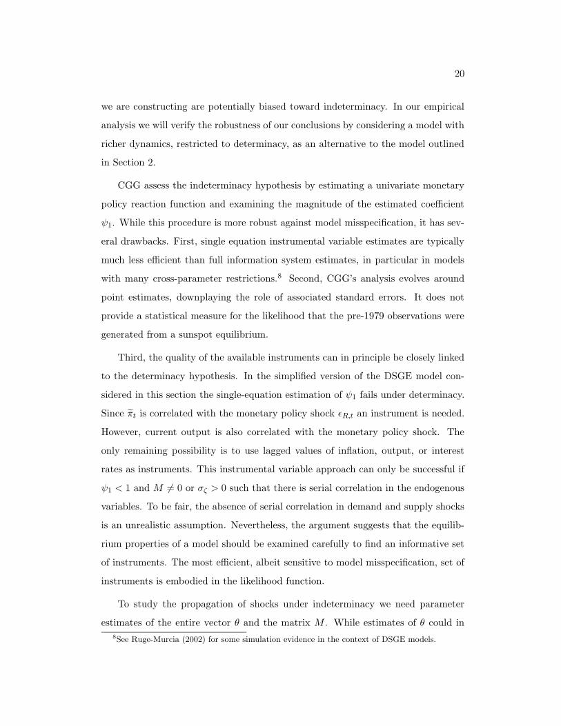
20
we are constructing are potentially biased toward indeterminacy. In our empirical
analysis we will verify the robustness of our conclusions by considering a model with
richer dynamics, restricted to determinacy, as an alternative to the model outlined
in Section 2.
CGG assess the indeterminacy hypothesis by estimating a univariate monetary
policy reaction function and examining the magnitude of the estimated coefficient
ψ1. While this procedure is more robust against model misspecification, it has sev-
eral drawbacks. First, single equation instrumental variable estimates are typically
much less efficient than full information system estimates, in particular in models
with many cross-parameter restrictions.8 Second, CGG’s analysis evolves around
point estimates, downplaying the role of associated standard errors. It does not
provide a statistical measure for the likelihood that the pre-1979 observations were
generated from a sunspot equilibrium.
Third, the quality of the available instruments can in principle be closely linked
to the determinacy hypothesis. In the simplified version of the DSGE model con-
sidered in this section the single-equation estimation of ψ1 fails under determinacy.
Since πt is correlated with the monetary policy shock εR,t an instrument is needed.
However, current output is also correlated with the monetary policy shock. The
only remaining possibility is to use lagged values of inflation, output, or interest
rates as instruments. This instrumental variable approach can only be successful if
ψ1 < 1 and M 6= 0 or σζ > 0 such that there is serial correlation in the endogenous
variables. To be fair, the absence of serial correlation in demand and supply shocks
is an unrealistic assumption. Nevertheless, the argument suggests that the equilib-
rium properties of a model should be examined carefully to find an informative set
of instruments. The most efficient, albeit sensitive to model misspecification, set of
instruments is embodied in the likelihood function.
To study the propagation of shocks under indeterminacy we need parameter
estimates of the entire vector θ and the matrix M . While estimates of θ could in
8See Ruge-Murcia (2002) for some simulation evidence in the context of DSGE models.

21
principle be obtained based on generalized method of moments estimates of Equa-
tions (1) to (3) subject to the availability of appropriate instruments, the estimation
of M requires a full-information approach such as the one proposed in this paper.
6 Empirical Results
The log-linearized monetary DSGE model described in Section 2 is fitted to quarterly
post-war U.S. data on output, inflation, and nominal interest rates.9 Both inflation
and interest rates are annualized. To make our empirical analysis comparable to
other studies, such as CGG, we use the HP filter to remove a smooth trend from
the output series. Results based on linear trend extraction are briefly discussed at
the end of this section. In line with the monetary policy literature we consider the
following sample periods: a pre-Volcker sample from 1960:I to 1979:II, a Volcker-
Greenspan sample from 1979:III to 1997:IV, and a post-1982 sample from 1982:IV
to 1997:IV that excludes the Volcker-disinflation period.
Inflation in the pre-Volcker years is marked by a substantial upward shift and
increase in volatility for which a variety of explanations have been offered. Or-
phanides (2002) suggests that the Federal Reserve misjudged trend productivity
growth in the 1970s and overestimated potential output. Since actual output ap-
peared relatively low the Fed loosened its monetary policy which led to high inflation.
Sargent (1999) argues that a perceived inflation-output trade-off could have led cen-
tral bankers to raise inflation targets. In the absence of an actual trade-off this
policy caused mainly high inflation rates. Other authors blame oil price shocks for
the rise in inflation. A fourth explanation for the experience in the pre-Volcker years,
set forth for instance by CGG, is that passive monetary policy failed to suppress
self-fulfilling inflation expectations. In the early 1980s the Fed switched to an active
9The time series are extracted from the DRI·WEFA database. Output is log real per capita
GDP (GDPQ), HP detrended over the period 1955:I to 1998:IV. We multiply deviations from
trend by 100 to convert them into percentages. Inflation is annualized percentage change of CPI-U
(PUNEW). Nominal interest rate is average Federal Funds Rate (FYFF) in percent.

22
monetary policy, raising the real interest rate in response to inflation deviations
from target, thus eliminating fluctuations due to self-fulfilling expectations.
Our simple monetary model is not detailed enough to completely disentangle
the four competing hypotheses. For instance, the central bank does not have to
solve a signal extraction problem that could capture the notion of mis-measured
potential output. Nevertheless, we can gain some interesting insights. Our analysis
is based on the assumption that the target inflation rate, which equals the steady
state inflation rate, stayed constant in the pre-Volcker years but possibly shifted in
the early 1980s as steady state inflation is estimated for each subsample separately.
Although the New Keynesian model does not distinguish energy and goods prices,
it has the ability to capture oil price shocks as drops in zt which, broadly speaking,
shift marginal costs of production. By estimating the DSGE model over both the
determinacy and indeterminacy region of the parameter space we can assess the
hypothesis of passive-monetary policy and self-fulfilling expectations and study the
propagation of fundamental and sunspot shocks under indeterminacy for the pre-
Volcker as well as the Volcker-Greenspan years.
Observed output deviations from trend, inflation, and interest rates are stacked
in the vector yt. The measurement equation that relates yt to the vector of model
variables st is of the form:
yt =
0
π∗
r∗ + π∗
+
1 0 0 0 0 0 0
0 4 0 0 0 0 0
0 0 4 0 0 0 0
st, (35)
where π∗ and r∗ are annualized steady state inflation and real interest rates (per-
centages). Abstracting from the small effect of long-run output growth on the
relationship between the discount factor β that appears in Equation (1) and r∗ we
replace the discount factor by β = (1+r∗/100)−1/4. The measurement equation (35)
together with the law of motion (26) for st provide a state-space model for the ob-
servables yt. The Kalman filter (see, for instance, Hamilton (1994)) can be used
to evaluate the likelihood function L(θ,M, σ|Y T ). This likelihood function is com-
bined with a prior distribution for the parameters θ, M , and σζ and computational

23
methods described in the Appendix are used to conduct posterior inference.
The empirical analysis is structured as follows. We first review the prior dis-
tribution, then present posterior probabilities for determinacy versus indeterminacy
together with estimates of all the model parameters. To gain insights into the prop-
agation of shocks we study impulse response functions and variance decompositions
under indeterminacy. Finally, we assess the robustness of our analysis to model
specification and detrending method.
6.1 Prior Distribution
The specification of the prior distribution is summarized in Table 1, which reports
prior densities, means, standard deviations, and 90% probability intervals for the
elements of θ, M , and σζ .10 It is assumed that the parameters are a priori indepen-
dent. In choosing priors for the policy parameters we adopted an agnostic approach.
The prior for the inflation coefficient ψ1 is centered at 1.1 and implies a probability
interval from 0.35 to 1.85. The interval for the output gap coefficient ψ2 ranges from
0.5 to 0.45. The degree of interest rate smoothing lies between 17% and 83%.
Our prior for the annual real interest rate is centered at 2% with a standard
deviation of 1. Steady state inflation ranges from 1% to 7%. The slope coefficient
in the Phillips-curve is chosen to be consistent with the range of values typically
found in the New-Keynesian Phillips-curve literature (see, for instance, Rotemberg
and Woodford (1997), Galı and Gertler (1999), and Sbordone (2002)). Its mean is
set at 0.5, but we allow the slope to vary widely in the unit interval. The prior for
1/τ is centered at 2, which makes the representative agents in the underlying model
more risk averse than agents with log-utility. The intervals for the autocorrelation
parameters ρg and ρz imply a fairly high degree of persistence of the exogenous
processes.
10Subsequent interval statements about parameters have the following interpretation: we report
the shortest (connected) intervals that have – according to our prior/posterior – a 90% coverage
probability.

24
The coefficients of the matrixM that appear in the indeterminacy solution have
standard normal distributions. Thus, our prior is centered at the baseline solution
described in Section 4. The prior for M , and the parameters that characterize
the distribution of the exogenous shocks are best assessed indirectly through their
implications for the volatility of output, inflation, and interest rates. Our prior
implies that the contribution of the monetary policy shock to output fluctuations
lies between 0 and 18%. Supply and demand shocks εa,t and εz,t may explain as
little as 1% or as much as 80% of the output variation. The sunspot shock εζ,t plays
hardly any role for output fluctuations but may cause up to 10% of the variation in
inflation and nominal interest rates. According to our prior the standard deviation
of inflation lies between 1% and 16%, which indicates that the prior for M assigns
some mass in regions of the parameter space that imply a large effect of fundamental
shocks on price movements.
We refer to the prior distribution described in Table 1 as Prior 1. Prior 2 is
obtained by imposing M = 0 and restricting the likelihood function in the indeter-
minacy region to the baseline solution described in Section 4. A third prior imposes
σζ = 0, which means that there are no sunspot shocks under indeterminacy so that
only the propagation of structural shocks is affected.
6.2 Estimation Results
The DSGE models is estimated under Priors 1 to 3 for the three samples. We will
first examine the probability mass assigned to the determinacy and indeterminacy
region. According to the priors the probability of determinacy is 0.527. One advan-
tage of our framework is that it lets us take into account the possible dependence
of the determinacy region on all elements of the parameter vector θ. To obtain the
posterior probabilities for the two regions of the parameter space it is convenient to
define the following (marginal) data densities
ps(Y T ) =
∫θ ∈ ΘsL(θ,M, σζ |Y
T )p(θ,M, σζ)dθ · dM · dσζ s ∈ D, I (36)

25
by integrating the likelihood function over region s with respect to the parameters
θ, M , and σζ .11 It can be seen from Equations (16) and (17) that the posterior
probability of indeterminacy is given by
πT (I) =pI(Y T )
pI(Y T ) + pD(Y T ). (37)
Table 2 reports ln ps(Y T ) and the resulting posterior probabilities by prior and
subsample.
The posterior probabilities reveal striking differences between the three subsam-
ples. The pre-Volcker posterior concentrates (almost) all of its probability mass
in the indeterminacy region. The evidence from the Volcker-Greenspan sample is
mixed. Depending on the choice of prior the probability of determinacy ranges from
0.38 to 0.7. These estimates could be strongly influenced by the Volcker disinflation
period which is better characterized by nonborrowed-reserve targeting than by an
interest rate rule. The inflation rate drops from 15% in 1980:I to about 6% in 1982.
Hence, the a sample which excludes the disinflation period is considered as an al-
ternative. Under all three priors the posterior probability of determinacy is around
0.98 for the post-1982 sample.
The log-data densities of Table 2 can also be used to compare the different
specifications of the DSGE model under indeterminacy. Under Prior 2 the model
is restricted to the baseline indeterminacy solution. The odds of the unrestricted
version (Prior 1) versus the M = 0 version (Prior 2) are 2 to 1 for the pre-Volcker
sample and 1.5 to 1 for the post-1982 sample. This finding suggests that the fit of
the model can be improved by deviating from the baseline solution and altering the
propagation of the structural shocks. Under Prior 3 the variance of the sunspot shock
is restricted to zero. Thus, agents do not react to an additional source of uncertainty.
The only effect of indeterminacy is to change the transmission of structural shocks.
For all three samples the ‘indeterminacy without sunspots’ version of the model
(Prior 3) is weakly preferred to the unrestricted specification.
11The data density intrinsically penalizes the likelihood function under indeterminacy for the
presence of the additional parameters M and σζ . The Schwarz (1978) approximation of a Bayesian
data density makes the penalty explicit.

26
Table 3 contains posterior estimates of the structural parameters for the pre-
Volcker sample (Prior 1, Prior 2) conditional on indeterminacy and for the post-
1982 sample conditional on determinacy. The post-1982 posterior indicates that
the monetary policy followed the Taylor principle. According to the posterior mean
the central bank raises the nominal rate by 2.2% in response to a 1% discrepancy
between actual and desired inflation. Active inflation targeting is supported by a
substantial degree of output gap targeting (ψ2 = 0.3) and interest rate smoothing
(ρR = 0.84).
Depending on the choice of prior the pre-Volcker sample leads to estimates of
ψ1 around 0.8 to 0.9. The Bayesian confidence sets for ψ2 range from 0.05 to 0.3.
The estimated steady state inflation rate appears slightly larger for the pre-Volcker
than for the post-1982 samples. However, there is substantial uncertainty about π∗.
The real rate was markedly lower before 1980, between 0.6% and 1.6%, than post
1982 when it was between 2.2% and 3.8% according to our posterior. The posterior
mean estimate of the slope κ of the Phillips curve is 0.77 with a confidence interval
ranging from 0.4 to 1.1 which is on the high side, but not unreasonably so.
Under Prior 2 (pre-Volcker) the estimated correlation between the shocks εg,t
and εz,t appears unreasonably large as it implies almost perfect correlation. Other
estimates of the covariance parameters as well as the vector M that determines
the relationship between fundamental shocks and forecast errors are best discussed
in the context of impulse response functions (IRF) and variance decompositions.
Recall that conditional on determinacy the likelihood function is invariant to M
and σζ . Hence the posterior distribution for these parameters is identical to the
prior distribution and the corresponding entries for Table 3 are left blank.
6.3 Propagation of Shocks
The system-based estimation approach pursued in this paper allows us to study the
propagation of fundamental and sunspot shocks in the model. Figure 2 graphs the
posterior mean responses (and pointwise 90% confidence bands) of output, inflation

27
and interest rates to a (negative) one-standard-deviation sunspot shock. The re-
sponses are based on the pre-Volcker posterior obtained under Prior 1. Under an
inflationary sunspot belief the expected real rate declines and the expected output
growth is negative. The fall in the real rate stimulates current consumption and
therefore output. According to the Phillips curve, this is consistent with positive
current inflation which validates the initial assumption of sunspot-driven positive
inflation expectations. As inflation falls toward its steady state in subsequent peri-
ods, the positive interest rate policy keeps the real rate low and output returns to
its steady state.. According to our estimates the sunspot shock has a much bigger
effect on inflation and interest rates than it has on output. Since both output and
inflation rise the sunspot shock cannot be interpreted as stagflation shock during
the 1970s in itself.
Figure 3 depicts the propagation of a monetary policy shock. Impulse responses
are computed based on three different parameter estimates, all based on the pre-
Volcker sample: (i) conditional on indeterminacy under Prior 1, (ii) conditional
on indeterminacy under Prior 2, and (iii) conditional on determinacy. The esti-
mated indeterminacy responses under Prior 2 are hardly distinguishable from the re-
sponses under indeterminacy. This suggests that the baseline solution around which
our prior is centered extends the determinacy solution to the indeterminacy region
without substantially altering the propagation of the fundamental shocks. In the
absence of the M = 0 restriction the estimated indeterminacy responses differ from
the baseline responses and reflect the non-zero estimates of M = [MRζ ,Mgζ ,Mzζ ]
reported in Table 3. Since MRζ is negative the propagation of εR,t is given by a
linear combination of the baseline IRFs and an inflationary sunspot shock as shown
in Figure 2.
Overall, in response to an unanticipated tightening of monetary policy output
drops initially by 0.15%, the interest rate rises by 70 basis points and inflation
falls 0.5% below steady state. Subsequently, inflation rises to about 0.2% whereas
output and inflation return to their steady states. Thus, according to our pre-
Volcker estimates under Prior 1, an increase in the nominal rate can have a slightly

28
inflationary effect. Figure 3 highlights that indeterminacy can alter the propagation
of fundamental shocks. Since the estimate of Mrζ is fairly imprecise the confidence
bands for the inflation and interest rate responses are wide. Given the the odds of
unrestricted M versus M = 0 are roughly 2 to 1 there is a substantial degree of
uncertainty about the effects of a monetary policy shock, even conditional on our
tightly parameterized DSGE model.
The shock εg,t shifts the consumption Euler equation and can broadly be inter-
preted as demand shock. Under determinacy a positive shock εg,t raises both output
and inflation. The positive estimate of Mgζ indicates that in the unrestricted inde-
terminacy version of the model the demand shock is less inflationary than under the
M = 0 indeterminacy solution. A positive supply shock εz,t reduces the marginal
costs of production, increases output and lowers inflation. The presence of inde-
terminacy creates an inflationary effect of εz,t since Mzζ is negative. The impulse
response functions for the Euler-equation and Phillips-curve shocks are depicted in
Figures 4 and 5.
Variance decompositions for output (deviations from trend), inflation, and inter-
est rates are summarized in Table 4. For the pre-Volcker sample we report posteriors
conditional on indeterminacy under Priors 1 and 2. The posterior for the post-1982
sample is conditional on determinacy. Since we allow εg,t and εz,t to have non-zero
correlation we need to orthogonalize the two shocks before computing variance de-
compositions. We assume that the orthogonalized supply shock only affects εz,t,
whereas the orthogonalized demand shock shifts both the Euler equation as well as
the price-setting equation. The rationale for this assumption is that shocks to the
marginal utility of consumption affect the labor supply decision and, in equilibrium,
the wage rate which is a component of marginal costs.
According to our posterior estimates neither monetary policy shocks nor sunspot
shocks have a notable impact on output fluctuations. Since the estimated correlation
between εg,t and εz,t under Prior 2 conditional on indeterminacy is near one, the
M = 0 version of the model attributes almost all of the output fluctuations to the
orthogonalized demand shock. The unrestricted pre-Volcker estimates as well as the

29
post-1982 estimates imply that most of the output fluctuations are due to shocks
that only affect the marginal costs of production. If M is restricted to zero then
the sunspot shock ζt explains between 50% and 90% of the variation in inflation
and nominal interest rates in the pre-Volcker period. Without this restriction the
contribution drops to 0 to 15%.
In summary, our empirical results shows that post 1982 monetary policy is
sufficiently anti-inflationary to rule out any indeterminacy. The pre-Volcker years,
however, were characterized by a monetary policy that violated the Taylor-principle.
According to the New Keynesian DSGE model this policy led to indeterminacy of
aggregate business cycle dynamics. Indeterminacy has two effects: the propagation
of fundamental shocks is not uniquely determined and sunspot shocks that are unre-
lated to the fundamental shocks may affect business cycle fluctuations. We consider
priors that assign different weights to the two effects. Someone who believes that
the propagation of the fundamental shocks is similar under determinacy and inde-
terminacy (Prior 2) will conclude that sunspot shocks explain a sizeable fraction
of inflation and interest rate variation. Someone who believes that indeterminacy
may fundamentally alter the propagation of structural shocks via the expectation
formation mechanism (Prior 1) will conclude that sunspots have played only a small
(or no) role as a source of business cycle fluctuations.
6.4 Robustness Analysis
We argued in Sections 4 and 5 that LRE models generate richer dynamics under
indeterminacy than determinacy because fewer autoregressive roots are suppressed.
The posterior weight on the determinacy region is based on the one hand on the
autocorrelation pattern in the observed data and on the other hand on the infor-
mation contained in the cross-coefficient restrictions implied by the DSGE model.
If the DSGE model lacks important propagation mechanisms that can generate suf-
ficiently rich dynamics than the posterior distribution of its parameters might be
unduly biased toward the indeterminacy region. Hence, as a robustness check we will

30
estimate a model with less restrictive dynamics than the standard New Keynesian
model presented in Section 2.
A more elaborate consumption Euler equation can be obtained by introducing
habit formation. Equation (1) can be derived from a period utility function in which
consumption Ct enters as
uC,t =C
1−1/τt
1− 1/τ. (38)
Previous research has found evidence that consumption relative to a habit stock
rather than the level of consumption itself should enter the period utility function.
Hence, we follow Fuhrer (2000) and introduce multiplicative habit formation. We
consider a period utility function of the form
uC,t =[Ct/C
γt−1]
1−1/τ
1− 1/τ, (39)
which for γ = 0 reduces to (38). The term Cγt−1 can be interpreted as habit stock.
It can be shown that the introduction of habit leads to the following modified Euler
equation:12
[τ +
1 + βγ2 + γ
1− βγ(1− τ)
]xt
=γ(1− τ)
1− βγxt−1 +
[τ +
1 + βγ(1 + γ)
1− βγ(1− τ)
]IEt[xt+1] (40)
−βγ
1− βγ(τ − 1)IEt+2[xt+2]− τ(Rt − IEt[πt+1]) + gt,
which for γ = 0 reduces to Equation (1).
The price setting equation (2) can be derived from the assumption that only
a fraction of monopolistically competitive firms is able to reoptimize their price in
response to shocks in any given period while the remaining firms adjust their prices
according to the steady state inflation rate. It is well known that (2) is unable to
endogenously generate the observed persistence in inflation. Gali and Gertler (1999)
propose a hybrid Phillips curve that involves lagged inflation on the right-hand side:
πt =β
1 + βωIEt[πt+1] +
ω
1 + βωπt−1 +
κ
1 + βω(xt − zt). (41)
12The derivation is relegated to a Technical Appendix that is available upon request.

31
Such an equation can be justified by assuming that a fraction ω of the firms that are
unable to reoptimize their price in a given period adjust their price charged in the
previous period by the lagged inflation rate rather than the steady state inflation
rate.
We estimated a LRE model based on Equations (40), (41), (3), and (4). Our
prior for ω is uniform on the interval [0, 1] whereas γ is distributed according to a
Gamma-distribution with mean 1 and standard deviation 0.4. Preliminary estimates
indicated that the simple price setting equation (ω = 0) is preferred to the hybrid
Phillips curve. In the estimates for the pre-Volcker sample reported in Table 5 we
impose the restriction ω = 0. According to the posterior distribution the habit
persistence parameter γ lies between 0.35 and 0.8. The estimates of the remaining
parameters are by and large in line with the estimates reported for the standard
New Keynesian model in Table 3.
Most interesting is whether the enriched model overturns our findings with re-
spect to the indeterminacy hypothesis. Log-data densities for the habit specification
conditional on determinacy are reported in Table 6. We revisit the pre-Volcker and
the Volcker-Greenspan sample. For both samples the habit model fits better than
the no-habit specification restricted to determinacy. The last column of Table 6
contains posterior probabilities for a comparison of the habit model restricted to
the determinacy region and the no-habit version estimated over both the determi-
nacy and the indeterminacy region. For the pre-Volcker sample the standard model
under indeterminacy provides a better description of the data than the richer model
restricted to the determinacy region. Thus, the conclusion of Section 2 with respect
to indeterminacy is not overturned.
For the Volcker-Greenspan sample the posterior of the no-habit model assigned
roughly equal weight to the determinacy and indeterminacy region of the parameter
space. The log-data density for the habit specification suggests that the evidence
for indeterminacy is not robust and can be overturned by the inclusion of additional
dynamics into the DSGE model.
As a second robustness check we estimate the standard version of the monetary

32
DSGE model based on output data that are linearly detrended instead of HP de-
trended. While the output deviations around this less flexible trend are larger and
more persistent our overall conclusion does not change. Post 1982 monetary policy
is sufficiently anti-inflationary to rule out indeterminacy. The pre-Volcker years,
however, monetary policy was passive which led according to the New Keynesian
DSGE model to indeterminacy.
7 Conclusion
We estimate a monetary business cycle model of the U.S. economy where monetary
policy is characterized by an interest rate rule that attempts to stabilize output and
inflation deviations around their target levels. It is well known that the applica-
tion of such a rule may lead to (local) indeterminacy, thus opening the possibility
of sunspot-driven aggregate fluctuations. Although previous research has acknowl-
edged this problem and made some attempts to deal empirically with indeterminacy,
our paper is, to the best of our knowledge, the first theoretically and empirically
consistent attempt to estimate a DSGE model without restricting the parameters
to the determinacy region.
Using a Bayesian approach we construct posterior weights for the determinacy
and indeterminacy regions of the parameter space. Our procedure takes into account
the dependence of the regions on all structural parameters and not just the policy
parameters. Moreover, our approach allows us to study the effect of indeterminacy
on the propagation of fundamental shocks and the importance of sunspot shocks for
aggregate fluctuations.
Empirical results confirm earlier studies that the behavior of the monetary au-
thority has changed beginning with the tenure of Paul Volcker as Federal Reserve
Chairman in 1979. During the Volcker-Greenspan years policy reacts very aggres-
sively towards inflation which puts the U.S. economy into the determinacy region.
On the other hand, monetary policy was much less active in the pre-Volcker period,
and through the lens of a standard New Keynesian DSGE model we cannot reject

33
the possibility of equilibrium indeterminacy. The DSGE model in this paper, albeit
widely employed in the recent monetary policy literature, is highly stylized. Its
overall time series fit is worse than that of a vector autoregression. Nevertheless, we
believe that some interesting lessons have been learned from our empirical analysis.
A fruitful avenue for future research is to apply our methods to models in which
determinacy is not as closely tied to the degree of activism as in the standard New
Keynesian DSGE model.
References
Andrews, Donald W.K. and Werner Ploberger (1994): “Optimal Tests when a
Nuisance Parameter is Present only under the Alternative,” Econometrica,
62, 1383-1414.
Blanchard, Olivier J. and Charles M. Kahn (1980): “The Solution of Linear Dif-
ference Models under Rational Expectations,” Econometrica, 48, 1305-1311.
Bullard, James and Kaushik Mitra (2002): “Learning about Monetary Policy
Rules,” Forthcoming: Journal of Monetary Economics.
Christiano, Lawrence J. and Sharon G. Harrison (1999): “Chaos, Sunspots, and
Automatic Stabilizers,” Journal of Monetary Economics, 44, 3-31.
Clarida, Richard, Jordi Galı, Mark Gertler (2000): “Monetary Policy Rules and
Macroeconomic Stability: Evidence and Some Theory,” Quarterly Journal of
Economics, 115(1), 147-180.
Cooper, Russell W. (2001): “Estimation and Indentification of Structural Parame-
ters in the Presence of Multiple Equilibria,” Manuscript, Department of Eco-
nomics, Boston University.
Dupor, Bill (2001): “Investment and Interest Rate Policy,” Journal of Economic
Theory, 98, 85-113.

34
Farmer, Roger E. A. and Jang-Ting Guo (1994): “Real Business Cycles and the
Animal Spirits Hypothesis,” Journal of Economic Theory, 63, 42-72.
Farmer, Roger E. A. and Jang-Ting Guo (1995): “The Econometrics of Indeter-
minacy: An Applied Study,” Carnegie-Rochester Conference Series on Public
Policy, 43, 225-271.
Fernandez-Villaverde, Jesus and Juan Francisco Rubio-Ramirez (2001): “Compar-
ing Dynamic EquilibriumModels to Data,”Manuscript, University of Pennsyvla-
nia.
Fuhrer, Jeffrey C. (2000): “Habit Formation in Consumption and Its Implications
for Monetary-Policy Models,” American Economic Review, 90, 367-390.
Galı, Jordi and Mark Gertler (1999): “Inflation Dynamics: A Structural Econo-
metric Analysis,” Journal of Monetary Economics, 44(2), 195-222.
Geweke, John F. (1999): “Using Simulation Methods for Bayesian Econometric
Models: Inference, Development, and Communication,” Econometric Reviews,
18, 1-126.
Hamilton, James D. (1994): “Time Series Analysis,” Princeton University Press,
Princeton.
Hannan, E.J. (1980): “The Estimation of the Order of an ARMA Process,” Annals
of Statistics, 8, 1071-1081.
Ireland, Peter N. (2001): “Sticky-Price Models of the Business Cycle: Specification
and Stability,” Journal of Monetary Economics, 47, 3-18.
Jovanovic, Boyan (1989): “Observable Implications of Models with Multiple Equi-
libria,” Econometrica, 57, 1431-1438.
Kim, Jae-Young (1998): “Large Sample Properties of Posterior Densities, Bayesian
Information Criterion, and the Likelihood Principle in Nonstationary Time
Series Models,” Econometrica, 66, 359-380.

35
Kim, Jinill (2000): “Constructing and Estimating a Realistic Optimizing Model of
Monetary Policy,” Journal of Monetary Economics, 45(2), 329-359.
King, Robert G. (2000): “The New IS-LM Model: Language, Logic, and Limits,”
Federal Reserve Bank of Richmond Economic Quarterly, 86(3), 45-103.
Leeper, Eric M. and Christopher A. Sims (1994): “Toward a Modern Macroe-
conomic Model Useable for Policy Analysis,” in: Stanley Fischer and Julio
Rotemberg (eds.) Macroeconomics Annual, MIT Press, Cambridge.
Lubik, Thomas A. and Massimiliano Marzo (2003): “An Inventory of Monetary
Policy Rules in a Simple, New-Keynesian Macroeconomic Model,”Manuscript,
Department of Economics, Johns Hopkins University.
Lubik, Thomas A. and Frank Schorfheide (2003): “Computing Sunspots in Linear
Rational Expectations Models,” Journal of Economic Dynamics and Control,
forthcoming.
McCallum, Bennett T. (1983): “On Nonuniqueness in Linear Rational Expecta-
tions Models: An Attempt at Perspective,” Journal of Monetary Economics,
11, 134-168.
Orphanides, Athanasios (2002): “Activist Stabilization Policy and Inflation: The
Taylor Rule in the 1970s,” Working Paper, Board of Governors.
Perli, Roberto (1998): “Indeterminacy, Home Production, and the Business Cycle:
A Calibrated Analysis,” Journal of Monetary Economics, 41, 105-125.
Phillips, Peter C.B. (1996): “Econometric Model Determination,” Econometrica,
64, 763-812.
Poirier, Dale (1998): “Revising Beliefs in Nonidentified Models,” Econometric The-
ory, 14, 183-209.
Rabanal, Pau and Juan Francisco Rubio-Ramirez (2002): “Nominal versus Real
Wage Rigidities: A Bayesian Approach,” Manuscript, Federal Reserve Bank
of Atlanta.

36
Rotemberg, Julio and Michael Woodford (1997): “An Optimization-Based Econo-
metric Framework for the Evaluation of Monetary Policy,” NBER Macroeco-
nomics Annual, 12, 297-246.
Ruge-Murcia, Francisco (2002): “Methods to Estimate Dynamic Stochastic Gen-
eral Equilibrium Models,” Discussion Paper, 2002-18, Department of Eco-
nomics, University of California at San Diego.
Salyer, Kevin D. and Steven M. Sheffrin (1998): “Spotting Sunspots: Some Evi-
dence in Support of Models with Self-Fulfilling Prophecies,” Journal of Mon-
etary Economics, 42, 511-523.
Sargent, Thomas J. (1999): “The Conquest of American Inflation,” Princeton
University Press, Princeton.
Sbordone, Argia M. (2002): “Prices and Unit Labor Costs: A New Test of Price
Stickiness,” Journal of Monetary Economics, 49, 265-292.
Schmitt-Grohe, Stephanie (1997): “Comparing Four Models of Aggregate Fluctu-
ations due to Self-Fulfilling Fluctuations,” Journal of Economic Theory, 72,
96-147.
Schmitt-Grohe, Stephanie (2000): “Endogenous Business Cycles and the Dynamics
of Output, Hours, and Consumption,” American Economic Review, 90(5),
1136-1159.
Schorfheide, Frank (2000): “Loss Function-Based Evaluation of DSGE Models,”
Journal of Applied Econometrics, 15, 645-670.
Schwarz, Gideon (1978): “Estimating the Dimension of a Model,” Annals of Statis-
tics, 6, 461-464.
Sims, Christopher A. (2002): “Solving Linear Rational Expectations Models,”
Computational Economics, 20, 1-20.
Woodford, Michael (2003): “Interest and Prices: Foundations of a Theory of Mon-
etary Policy,” Princeton University Press, forthcoming, Princeton.

37
A Practical Implementation
1. The matrices Γ0(θ), Γ1(θ), Ψ(θ), and Π(θ) of the canonical LRE model (5)
can be derived from Equations (1) to (4). Instead of inverting Γ0(θ) and using
a Jordan decomposition of Γ−10 Γ1 as described in Section 4, we proceed as in
Sims (2002) with a generalized complex Schur decomposition (QZ) of Γ0 and
Γ1. There exist matrices Q, Z, Λ, and Ω such that Q′ΛZ ′ = Γ0, Q′ΩZ ′ = Γ1,
QQ′ = Q′Q = ZZ ′ = Z ′Z = In×n and Λ and Ω are upper triangular. Let
wt = Z ′yt and premultiply (5) by Q to obtain
Λ11 Λ12
0 Λ22
w1,t
w2,t
=
Ω11 Ω12
0 Ω22
w1,t−1
w2,t−1
+
Q1.
Q2.
(Ψεt +Πηt).
(42)
The second set of equations can be rewritten as:
w2,t = Λ−122 Ω22w2,t−1 + Λ−1
22 Q2.(Ψεt +Πηt) (43)
Without loss of generality, we assume that the system is ordered and parti-
tioned such that the m× 1 vector w2,t is purely explosive, where 0 ≤ m ≤ n.
We apply the singular value decomposition (24) to Q2.Π instead of ΠJx and
obtain ηt according to Proposition 1, where ΨJx is replaced by Q2.Ψ. To find
M∗(θ) use (30), which leads to a vector autoregression law of motion for st.
2. Combine (26) with the measurement equation (35) to form a state space model
for the observables yt. The likelihood function L(θ,M, σζ |YT ) can be evaluated
with the Kalman Filter.
3. Let p(θ,M, σζ) and p(θ,M, σζ |YT ) denote prior and posterior densities of θ,
respectively. Since the likelihood function L(θ,M, σζ)|YT ) is discontinuous at
the boundary of the determinacy region we conduct the computations for the
two regions of the parameter space separately.
4. A numerical-optimization procedure is used to maximize
ps(θ,M, σζ |YT ) ∝ Ls(θ,M, σζ |Y
T )p(θ,M, σζ)θ ∈ Θs, s ∈ D, I

38
and find the posterior mode in the two regions of the parameter space. The
inverse Hessian is calculated at the posterior mode.
5. For each region, 1,000,000 draws from p(θ,M, σζ |YT ) are generated with a
random-walk Metropolis Algorithm. The scaled inverse Hessian serves as a co-
variance matrix for the Gaussian proposal distribution used in the Metropolis-
Hastings algorithm. If for a particular sample a region of the parameter space
does not have a (local) mode, we use the inverse Hessian obtained from one
of the other samples for that region. The first 100,000 draws are discarded.
The parameter draws θ are converted into impulse response functions and
variance decompositions to generate the results reported in Section 6. Pos-
terior moments are obtained by Monte-Carlo averaging. The marginal data
densities for the two regions are approximated with Geweke’s (1999) modified
harmonic-mean estimator. Further details of these computations are discussed
in Schorfheide (2000).

39
Table 1: Prior Distributions for DSGE Model Parameters
Name Range Density Mean Stdd 90% Interval
ψ1 IR+ Gamma 1.10 0.50 [ 0.33, 1.85]
ψ2 IR+ Gamma 0.25 0.15 [ 0.06, 0.43]
ρR [0,1) Beta 0.50 0.20 [ 0.18, 0.83]
π∗ IR+ Gamma 4.00 2.00 [ 0.90, 6.91]
r∗ IR+ Gamma 2.00 1.00 [ 0.49, 3.47]
κ IR+ Gamma 0.50 0.20 [ 0.18, 0.81]
τ−1 IR+ Gamma 2.00 0.50 [ 1.16, 2.77]
ρg [0.1) Beta 0.70 0.10 [ 0.54, 0.86]
ρz [0.1) Beta 0.70 0.10 [ 0.54, 0.86]
ρgz [-1,1] Normal 0.00 0.40 [-0.65, 0.65]
MRζ IR Normal 0.00 1.00 [-1.64, 1.64]
Mgζ IR Normal 0.00 1.00 [-1.64, 1.64]
Mzζ IR Normal 0.00 1.00 [-1.64, 1.64]
σR R+ Inv. Gamma 0.31 0.16 [ 0.13, 0.50]
σg R+ Inv. Gamma 0.38 0.20 [ 0.16, 0.60]
σz R+ Inv. Gamma 1.00 0.52 [ 0.42, 1.57]
σζ R+ Inv. Gamma 0.25 0.13 [ 0.11, 0.40]
Notes: The Inverse Gamma priors are of the form p(σ|ν, s) ∝ σ−ν−1e−νs2/2σ2, where
ν = 4 and s equals 0.25, 0.3, 0.6, and 0.2, respectively. The prior for ρgz is truncated
to ensure that the correlation lies between -1 and 1. We refer to the prior distribution
in this Table as Prior 1. Prior 2 is obtained by imposing MRζ = Mgζ = Mzζ = 0,
whereas Prior 3 imposes σζ = 0.
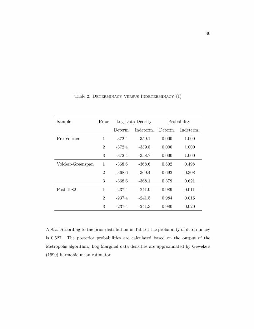
40
Table 2: Determinacy versus Indeterminacy (I)
Sample Prior Log Data Density Probability
Determ. Indeterm. Determ. Indeterm.
Pre-Volcker 1 -372.4 -359.1 0.000 1.000
2 -372.4 -359.8 0.000 1.000
3 -372.4 -358.7 0.000 1.000
Volcker-Greenspan 1 -368.6 -368.6 0.502 0.498
2 -368.6 -369.4 0.692 0.308
3 -368.6 -368.1 0.379 0.621
Post 1982 1 -237.4 -241.9 0.989 0.011
2 -237.4 -241.5 0.984 0.016
3 -237.4 -241.3 0.980 0.020
Notes: According to the prior distribution in Table 1 the probability of determinacy
is 0.527. The posterior probabilities are calculated based on the output of the
Metropolis algorithm. Log Marginal data densities are approximated by Geweke’s
(1999) harmonic mean estimator.
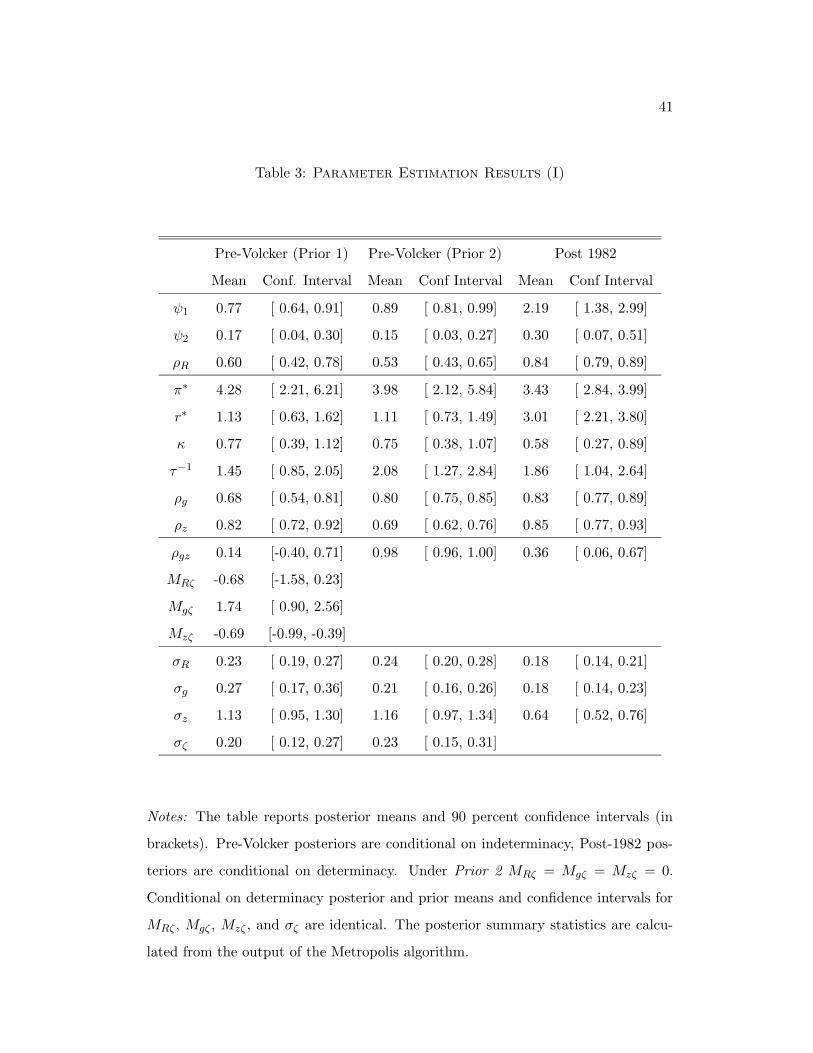
41
Table 3: Parameter Estimation Results (I)
Pre-Volcker (Prior 1) Pre-Volcker (Prior 2) Post 1982
Mean Conf. Interval Mean Conf Interval Mean Conf Interval
ψ1 0.77 [ 0.64, 0.91] 0.89 [ 0.81, 0.99] 2.19 [ 1.38, 2.99]
ψ2 0.17 [ 0.04, 0.30] 0.15 [ 0.03, 0.27] 0.30 [ 0.07, 0.51]
ρR 0.60 [ 0.42, 0.78] 0.53 [ 0.43, 0.65] 0.84 [ 0.79, 0.89]
π∗ 4.28 [ 2.21, 6.21] 3.98 [ 2.12, 5.84] 3.43 [ 2.84, 3.99]
r∗ 1.13 [ 0.63, 1.62] 1.11 [ 0.73, 1.49] 3.01 [ 2.21, 3.80]
κ 0.77 [ 0.39, 1.12] 0.75 [ 0.38, 1.07] 0.58 [ 0.27, 0.89]
τ−1 1.45 [ 0.85, 2.05] 2.08 [ 1.27, 2.84] 1.86 [ 1.04, 2.64]
ρg 0.68 [ 0.54, 0.81] 0.80 [ 0.75, 0.85] 0.83 [ 0.77, 0.89]
ρz 0.82 [ 0.72, 0.92] 0.69 [ 0.62, 0.76] 0.85 [ 0.77, 0.93]
ρgz 0.14 [-0.40, 0.71] 0.98 [ 0.96, 1.00] 0.36 [ 0.06, 0.67]
MRζ -0.68 [-1.58, 0.23]
Mgζ 1.74 [ 0.90, 2.56]
Mzζ -0.69 [-0.99, -0.39]
σR 0.23 [ 0.19, 0.27] 0.24 [ 0.20, 0.28] 0.18 [ 0.14, 0.21]
σg 0.27 [ 0.17, 0.36] 0.21 [ 0.16, 0.26] 0.18 [ 0.14, 0.23]
σz 1.13 [ 0.95, 1.30] 1.16 [ 0.97, 1.34] 0.64 [ 0.52, 0.76]
σζ 0.20 [ 0.12, 0.27] 0.23 [ 0.15, 0.31]
Notes: The table reports posterior means and 90 percent confidence intervals (in
brackets). Pre-Volcker posteriors are conditional on indeterminacy, Post-1982 pos-
teriors are conditional on determinacy. Under Prior 2 MRζ = Mgζ = Mzζ = 0.
Conditional on determinacy posterior and prior means and confidence intervals for
MRζ , Mgζ , Mzζ , and σζ are identical. The posterior summary statistics are calcu-
lated from the output of the Metropolis algorithm.

42
Table 4: Variance Decompositions
Pre-Volcker (Prior 1) Pre-Volcker (Prior 2) Post 1982
Mean Conf. Interval Mean Conf Interval Mean Conf Interval
Output Deviations from Trend
Policy 0.01 [ 0.00, 0.02] 0.01 [ 0.00, 0.02] 0.04 [ 0.01, 0.06]
Demand(*) 0.19 [ 0.00, 0.51] 0.97 [ 0.95, 0.99] 0.36 [ 0.09, 0.63]
Supply(*) 0.80 [ 0.47, 0.99] 0.01 [ 0.00, 0.03] 0.60 [ 0.33, 0.88]
Sunspot 0.00 [ 0.00, 0.01] 0.00 [ 0.00, 0.01] 0.00 [ 0.00, 0.00]
Inflation
Policy 0.08 [ 0.00, 0.18] 0.07 [ 0.02, 0.11] 0.29 [ 0.14, 0.43]
Demand(*) 0.23 [ 0.01, 0.46] 0.17 [ 0.03, 0.30] 0.47 [ 0.32, 0.63]
Supply(*) 0.59 [ 0.32, 0.87] 0.07 [ 0.00, 0.14] 0.24 [ 0.07, 0.40]
Sunspot 0.10 [ 0.01, 0.18] 0.70 [ 0.50, 0.92] 0.00 [ 0.00, 0.00]
Interest Rates
Policy 0.17 [ 0.00, 0.41] 0.08 [ 0.01, 0.15] 0.08 [ 0.03, 0.12]
Demand(*) 0.20 [ 0.00, 0.42] 0.16 [ 0.01, 0.29] 0.61 [ 0.38, 0.84]
Supply(*) 0.54 [ 0.25, 0.87] 0.05 [ 0.00, 0.10] 0.32 [ 0.12, 0.51]
Sunspot 0.08 [ 0.01, 0.15] 0.71 [ 0.51, 0.92] 0.00 [ 0.00, 0.00]
Notes: The table reports posterior means and 90 percent confidence intervals (in
brackets). The posterior summary statistics are calculated from the output of the
Metropolis algorithm. Since the estimated correlation between εg,t and εz,t is non-
zero we orthogonalize the demand and supply shock for this variance decomposition
using a triangular decomposition. We assume that the supply(*) shock only affects
εz,t.

43
Table 5: Parameter Estimation Results (II)
Pre-Volcker (Habit)
Mean Conf. Interval
ψ1 1.07 [ 1.00, 1.15]
ψ2 0.10 [ 0.02, 0.19]
ρR 0.59 [ 0.48, 0.72]
π∗ 4.53 [ 3.48, 5.57]
r∗ 1.14 [ 0.71, 1.57]
κ 0.66 [ 0.30, 1.01]
τ−1 1.58 [ 1.05, 2.15]
ω 0.00 [ 0.00, 0.00]
γ 0.57 [ 0.35, 0.79]
ρg 0.87 [ 0.83, 0.91]
ρz 0.79 [ 0.74, 0.85]
ρgz 0.93 [ 0.88, 0.97]
σR 0.26 [ 0.21, 0.30]
σg 0.18 [ 0.13, 0.23]
σz 1.29 [ 1.06, 1.53]
Notes: The table reports posterior means and 90 percent confidence intervals (in
brackets). Estimates of habit-specification are based on Pre-Volcker sample, condi-
tional on determinacy.

44
Table 6: Determinacy versus Indeterminacy (II)
Sample Spec Log Data Density Probability
Determ. Indeterm.
Pre-Volcker Prior 3 -372.4 -358.7 1.000
Habit -370.0 0.000
Volcker-Greenspan Prior 3 -368.6 -368.1 0.038
Habit -364.4 0.962
Notes: The posterior probabilities are calculated based on the output of the
Metropolis algorithm. Log Marginal data densities are approximated by Geweke’s
(1999) harmonic mean estimator.
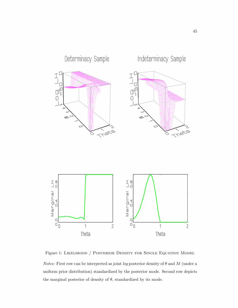
45
Figure 1: Likelihood / Posterior Density for Single Equation Model
Notes: First row can be interpreted as joint log posterior density of θ andM (under a
uniform prior distribution) standardized by the posterior mode. Second row depicts
the marginal posterior of density of θ, standardized by its mode.

46
Figure 2: Impulse Responses to Sunspot Shock
Notes: Pre-Volcker sample, indeterminacy region (Prior 1). Figure depicts posterior
means (solid lines) and pointwise 90% posterior confidence intervals (dashed lines)
for impulse responses of output, inflation, and the nominal interest rate to a one-
standard deviation shock εζ,t.
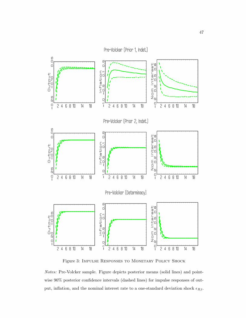
47
Figure 3: Impulse Responses to Monetary Policy Shock
Notes: Pre-Volcker sample. Figure depicts posterior means (solid lines) and point-
wise 90% posterior confidence intervals (dashed lines) for impulse responses of out-
put, inflation, and the nominal interest rate to a one-standard deviation shock εR,t.
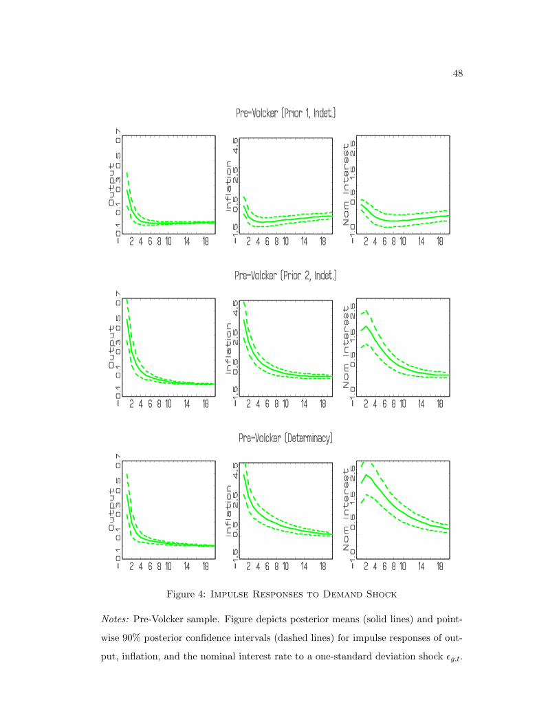
48
Figure 4: Impulse Responses to Demand Shock
Notes: Pre-Volcker sample. Figure depicts posterior means (solid lines) and point-
wise 90% posterior confidence intervals (dashed lines) for impulse responses of out-
put, inflation, and the nominal interest rate to a one-standard deviation shock εg,t.

49
Figure 5: Impulse Responses to Supply Shock
Notes: Pre-Volcker sample. Figure depicts posterior means (solid lines) and point-
wise 90% posterior confidence intervals (dashed lines) for impulse responses of out-
put, inflation, and the nominal interest rate to a one-standard deviation shock εz,t.