Running Head: single-case methods

Neuropsychology, in press

(Neuropsychology journal home page)

© American Psychological Association

This article may not exactly replicate the final version published in the APA journal. It is not the copy

of record

Testing for suspected impairments and dissociations in single-case studies

in neuropsychology: Evaluation of alternatives using Monte Carlo

simulations and revised tests for dissociations

John R. Crawford1 and Paul H. Garthwaite2

1School of Psychology

University of Aberdeen

Aberdeen, UK

2Department of Statistics

The Open University

Milton Keynes, UK

____________________________________

Address for correspondence: Professor John R. Crawford, School of Psychology, College of Life

Sciences and Medicine, King’s College, University of Aberdeen, Aberdeen AB24 2UB, United

Kingdom. E-mail: j.crawford@abdn.ac.uk

1

ABSTRACT

In many neuropsychological single-case studies a patient is compared to a small

control sample. Methods for testing whether the patient may have an impairment on

task X, or a significant difference between tasks X and Y, either treat the control

sample statistics as parameters (they use z, and z for the difference between X and Y,

i.e., Dz ) or they use modified t-tests. Monte Carlo simulations demonstrated that, if z

is used to test for a possible impairment, the Type I error rate is high for small control

samples, whereas control of the error rate is essentially perfect for a modified t-test.

Simulations on the tests for differences revealed that the error rates were very high for

Dz , particularly with small control sample Ns (e.g., over 20% for an N of 5). A

modified paired t-test achieved much better control but error rates were still above 5%

with small Ns. A revised version of the t-test that overcomes this limitation but still

permits standardization of a patient’s scores achieved good control of the error rate,

even with very small Ns (e.g. error rates ranged from 5.17% to 5.59% for N = 5).

Similarly, positive results were obtained for a revised test that can be employed when

it is legitimate not to standardize a patient’s scores. A computer program that

implements the new tests (and applies criteria for determining the presence of

classical and strong dissociations) is made available.

Key terms: single-case studies; statistical methods; dissociations

2

INTRODUCTION

In many single-case studies in neuropsychology the performance of a patient

on a series of tasks is compared to that of a control sample. By far the most common

method of forming inferences about the presence of a possible impairment in such

studies is to convert the patient’s score on a given task to a z-score based on the mean

and SD of the controls and then refer this score to a table of the areas under the

normal curve. Thus, if a neuropsychologist has formed a directional hypothesis for

the patient’s score prior to testing (i.e., that the patients score will be below the

control sample mean), then a score that fell below –1.645 would be considered

statistically significant (p < 0.05) and would be taken as an indication that the patient

had an impairment on the task in question.

One problem with this approach is that it treats the control sample as if it was

a population; i.e., the mean and standard deviation are used as if they were

parameters rather than sample statistics. In other areas of psychology this is often not

a problem in practice as the normative or control sample is large and therefore should

provide sufficiently accurate estimates of the parameters. However, the control

samples in single-case studies in cognitive neuropsychology typically have modest

Ns; N < 10 is not unusual and Ns < 20 are very common (Crawford & Howell, 1998).

With samples of this size it is not appropriate to treat the mean and SD as though they

were parameters.

A solution to this problem is to use a method described by Crawford and

Howell (1998) that treats the control sample statistics as sample statistics. Their

approach uses a formula for a modified t-test given by Sokal and Rohlf (1995). This

method uses the t-distribution (with n - 1 degrees of freedom), rather than the

standard normal distribution, to estimate the abnormality of the patient’s scores and to

3

test whether it is significantly lower than the scores of the control sample. The

practical effect of using z with small control sample is to exaggerate the rarity /

abnormality of a patient’s score and to inflate the Type I error rate (in this context a

Type I error occurs when a case that is drawn from the control population is

incorrectly classified as not being a member of this population; i.e. they are

incorrectly classified as exhibiting an impairment). This occurs because the normal

distribution has “thinner tails” than t-distributions. Intuitively, the less that is known,

the less extreme should be statements about abnormality/rarity. The z score method

treats the variance of controls as being known, when it is not, and consequently makes

statements that are too extreme (Crawford & Howell, 1998). The formula for

Crawford and Howell’s (1998) test is

*

1X Xt

nSn

−=

+, (1)

where *X is the patient’s score, X and S are the mean and standard deviation of

scores in the control sample and n is the size of the control sample. The p value

obtained when this test is applied is used to test significance but it also provides a

point estimate of the abnormality of the patient’s score; for example if the one-tailed p

is 0.013 then we know that the patient’s score is significantly (p < .05) below the

control mean and that it is estimated that 1.3% of the control population would obtain

a score lower than the patient’s. As Crawford and Howell (1998) note, this point

estimate of abnormality is a useful complement to the significance test given that the

use of an alpha of 0.05 is essentially an arbitrary convention (albeit one that has, in

general, served science well).

4

STUDY 1

Tests aimed at detecting an impairment when a case is compared to a control sample

In the first study we run a Monte Carlo simulation to quantify and compare

control of the Type I error rate when the two alternative methods of detecting an

impairment are used to compare individual control cases against control samples. The

statistically sophisticated reader may consider that running this simulation is

unnecessary because theory would predict that the use of z will fail to control Type I

errors whereas the modified t-test will achieve adequate control. However, we had

two reasons for conducting it. First, the use of z to detect an impairment in a patient

is very widespread (Crawford & Garthwaite, 2002; Crawford, Garthwaite, & Gray,

2003a) so clearly many researchers are either unaware, or have chosen to ignore, the

issue of inflated Type I errors. Quantifying the magnitude of this inflation may help

to raise awareness of the problem, and doing so using an empirical method may be

more convincing than appeal to theory alone.

Second, all readers will be familiar with the use of independent samples t-tests

to test for a difference in population means in which two samples are compared. In

this standard situation, variance estimates are obtained from the two samples and

these are pooled (or alternatively separate variance estimates are used when the

variances differ). However, many readers will not be familiar with the modified t-test

in which we need only (and can only) be concerned, with the variance estimate of the

control population. Under the null hypothesis the patient is an observation from a

distribution with the same mean and variance as the controls. Because, unlike a

standard t-test, the patient does not contribute to a pooled variance estimate (nor

contributes a separate variance estimate), readers may appreciate reassurance that

control of Type I errors is adequate in this non-standard use of a t-test.

5

Method

The Monte Carlo simulation was run on a PC and implemented in Borland

Delphi (Version 4). The algorithm ran3.pas (Press, Flannery, Teukolsky, &

Vetterling, 1989) was used to generate uniform random numbers (between 0 and 1)

and these were transformed by the polar variant of the Box-Muller method (Box &

Muller, 1958) to sample from a normal distribution. The simulation was run with five

different values of N (the sample size of the control sample): For each of these values

of N, 1,000,000 samples of items were drawn from a normal distribution. The

first N items in each sample were taken as the control sample and the item

taken as the individual control case. Crawford and Howell's (1998) test was then

applied to these data and t values that were negative (i.e., where the control case was

below the control sample) and exceeded the one-tailed critical value for t on the

appropriate degrees of freedom (

1N +

1thN +

1n− ) were recorded as Type I errors; z was also

computed and the result recorded as a Type I error if it exceeded the one-tailed

critical value of -1.645. One-tailed tests were employed because, in the vast majority

of cases, the (directional) hypothesis tested by neuropsychologists is that their

patient’s score is below that of controls.

Results and Discussion

The results of the Monte Carlo simulation are presented in Table 1. It can be

seen from Table 1 that, when the size of the control sample is small, control of the

Type I error rate is poor when z is used to test for a significant difference between a

case and controls. For example, the error rate is 10.37% with N of 5, more than

double the specified rate of 5%. Therefore, if z is used in a single-case study using a

6

control sample of N = 5, it is to be expected that over 10% of individuals from the

control population would be incorrectly identified as not having come from this

population (i.e., they would be considered to exhibit an impairment). With large Ns, z

values more closely approximate t values so that the error rate is under satisfactory

control. However, it will be appreciated that control sample Ns of this magnitude are

rare in single-case studies in neuropsychology.

__________________

Insert Table 1 about here __________________

In contrast to the inflated error rates when z is used, it can be seen that there is

immaculate control of the Type I error rate when the modified t-test is employed; the

error rates for all of the sample sizes examined are all at, or very close to, the

specified rate of 5% (the magnitude of the differences from 5% are of the order

expected solely from Monte Carlo variation.) Having verified empirically that the

Type I error rate is controlled when the modified t-test is employed we can use the

fact that the z-score satisfies

1nz tn+

= , (2)

to record the actual value of z that would be required to maintain the Type I error rate

at 5%. These values of z are presented in the final column of Table 1. It can be seen

that the values of z required to maintain the Type I error rate at the specified level are

markedly greater than the nominal critical value of 1.645− ; e.g., with a control

sample N of 5, a z of -2.335 would be required. This example also highlights the

extent to which z will tend to provide an exaggerated estimate of the rarity of a

patient’s score. Suppose a patient obtained a z score of –2.335; using a table of the

areas under the normal curve it would be estimated that 0.98% of the control

7

population would obtain a lower score (i.e. the patient’s score is estimated to be very

rare) yet the unbiased estimate provided by t is that 5% of the population would be

expected to obtain a lower score.

STUDY 2

The effects of skew in the control population on Type I error rates

An assumption underlying the use of z or Crawford and Howell’s test is that

the controls have been drawn from a normal distribution. However, it is not

uncommon for the scores of controls on neuropsychological tests to depart from

normality. In Study 2 we examine the effects on the Type I error rate of violating the

assumption of normality. For a number of reasons, the focus of this study is on the

effects of negative skew. One reason for concentrating on skewness is that, a priori,

skew is liable to have a greater effect on Type I errors than other forms of departure

from a normal distribution. This is because low-order moments are important (the

first-order moment is the mean and the second order moment is the variance), and

skewness is the lowest-order moment that does not correspond to a parameter of a

normal distribution. Also, empirical studies of error rates for independent samples

t-tests confirm that skew is the most important parameter (e.g., Boneau, 1960; see

Howell, 2002 for a brief review). In addition, it has been shown that the effect of

skew is particularly pronounced when combined with large imbalances in samples

sizes; as the present methods involve comparing an individual with a sample this

underlines the need to study this issue.

We focus on negative skew because it is clear that, in practice, the scores of

controls are often negatively skewed. As Crawford et al. (2003a) note, “z has been

used for inferential purposes in numerous single-case studies when it is obvious from

8

the means and SDs of their control samples that the data are highly negatively skewed

(i.e. the SD tells us that, were the data normally distributed, a substantial percentage

of scores should lie above the maximum obtainable score yet we know that none did)”

(p. 367). Negative skew is common in control data because the tasks employed often

measure abilities that are largely within the competence of most healthy individuals

and thus yield ceiling or near-ceiling levels of performance. For example, in a review

of single-case studies of the living versus non-living distinction in object naming, it

was reported that the accuracy of naming in controls was 95% or greater in the vast

majority of these studies (Laws, Gale, Leeson, & Crawford, in press).

It will be appreciated that when (as is less common) performance is expressed

as the number of errors on a task then the opposite situation to that described above

will often occur i.e. the distribution of scores for controls will be positively skewed.

However, by reflecting scores a positively skewed distribution can be converted into

an equivalently negatively skewed distribution, so results obtained in the present

study are equally applicable to scenarios in which the control scores are positively

skewed.

Method

Simulations were run using an identical approach to Study 1 except that,

instead of sampling from a normal distribution, observations were sampled from

distributions with varying degrees of negative skew. This was achieved by using

two-piece normal distributions (Gibbons & Mylroie, 1973; Kimber, 1985); these

distributions have also been termed joined half-Gaussian or binormal distributions. In

comparison to alternative methods of modelling the effects of skewness, two-piece

normal distributions have been shown to possess a number of desirable properties,

9

including their suitability when there is a requirement (as in the present study) to

draw small samples (Garvin & McClean, 1997).

Skewness is most commonly quantified using the statistic ; this statistic is

obtained by dividing the third central moment of a distribution by the cube of its

standard deviation. We formed four distributions that varied in their degree of skew

ranging from moderate ( = -0.31) to severe (-0.70), very severe (-0.93) and extreme

(-0.99). These distributions were obtained by setting the standard deviation of the

normal distribution used to form the right-hand side of the two-piece distribution to

1.0 and the SD of the normal distribution used for the left-hand side to values of 1.5,

3.0, 10.0, and 100.0 respectively. The resultant two-piece distributions are illustrated

in Figure 1. It can be seen that the degrees of skew for the latter two of these

distributions are exceptionally large, to the extent that the gross appearance of the

distribution with “extreme” skew is that of a normal distribution in which all of the

right-hand side is absent.

1g

1g

1,000,000 samples of pairs of observations were drawn from each of the

four skew distributions. As in Study 1, this was done for four values of N: 5, 10, 20,

50, and 100. Also as in Study 1, Crawford and Howell's (1998) test and z were

applied to the score of the N+1th control case and the result recorded as a Type I error

if it exceeded the respective one-tailed critical value.

1N +

__________________

Insert Table 2 about here __________________

Results and Discussion

The simulation results for z and for Crawford and Howell’s test are presented

in Table 2. It can be seen that when z is used to test for an impairment, the control of

10

the Type I error rate is poor; the error rates range from a low of 6.20% (N= 100

combined with moderate skew) to a high of 13.39% (N = 5 combined with extreme

skew). However, at the small control sample Ns commonly used in single-case

studies, the poor control of the error rate mainly stems from the treatment of the

control sample statistics as population parameters. That is, although the presence of

skewness has further inflated the error rate over that observed in Study 1, the

increment is relatively modest. For example, when sampling from a normal

distribution with an N of 5 the error rate was over twice the nominal rate of 5%

(10.37%) and even the presence of extreme skew only raised this error rate to

13.40%.

As noted, the effect of skew on t-tests has been examined in previous

simulation studies. However, in all these prior studies the focus was on the use of t to

test for a difference in population means. In contrast, Crawford and Howell’s

procedure tests the hypothesis that an individual patient did not come from a

population of controls; under the null hypothesis, the individual is an observation

from a distribution with the same mean and variance as the controls (Crawford,

Garthwaite, Howell, & Gray, in press). The effects of skew have therefore not been

previously investigated in this non-standard application of a t-test.

It can be seen from Table 2 that there is modest inflation of the Type I error

rate using Crawford and Howell’s test when skew is moderate or not very severe (e.g.,

for a control sample size of 10 the error rates are 6.04% for moderate and 7.14% for

severe skew). The Type I error rate rises as high as 8.27% when skew is extreme.

However, it is clear that the rate of increase in Type I error rate becomes attenuated as

the distributions become more severely skewed; the increase in the degree of skew

from very severe to extreme is substantial and yet the concomitant increase in the

11

Type I error rate is modest (e.g. with a control sample size of 10 the error rate is

7.80% for very severe skew and is 7.94% for extreme skew). It should also be

reiterated that the degree of skew in these latter two distributions is exceptionally

large.

Although the inflation of the Type I error rate is not very acute even with very

severe skew (i.e., the test is more robust than might have been predicted) it remains

the case that the error rate is not under control. Therefore some guidance should be

offered for researchers when it is suspected that control data are skew.

One potential alternative to Crawford and Howell’s parametric test would be

to use non-parametric tests (e.g. randomisation tests). However, there are two

limitations to this potential solution. First, these methods are, by necessity,

completely insensitive to the degree to which a patient’s score is extreme and

therefore will have low power (e.g., a patient whose score on a task was 8 SDs below

the control mean would be treated identically to a patient whose score was 2 SDs

below the mean provided that their rank order relative to controls was the same).

Power is inevitably low in single-case studies because an individual rather than a

sample is compared to a control sample that is itself typically modest in size;

therefore any treatment that imposes a further reduction in power should be avoided if

at all possible (Crawford et al., 2003a). Second, the size of sample required before a

researcher has any possibility of rejecting the null hypothesis of no difference

between patient and controls is larger than is typical in single-case studies. A

minimum of 20 controls would be required to be able to reject the null hypothesis

even when the alternative hypothesis is directional (p < .05, one-tailed) and such an

outcome would only occur if the score of every control was higher than the patient’s.

12

When the control data are skew one possibility would be to transform the

scores of controls and the patient in an attempt to normalise the control score

distribution. For example, in the case of moderate negative skew the scores could be

reflected and a logarithmic transformation applied (for further guidance see Howell,

2002). Alternatively, however, even if Crawford and Howell’s test is applied to

untransformed scores, the researcher can still have a high degree of confidence that

the patient’s score did not come from the control distribution if the result is highly

significant. That is, even with very severe skew, the observed error rate for a

specified rate of 5% never rose above 8.27%; thus t values that are markedly larger

than the critical value would be sufficient to warrant rejection of the null hypothesis.

To study this suggestion more formally we re-ran the simulation (for Crawford &

Howell’s test alone given its demonstrated superiority over the use of z in both this

study and Study 1) but substituted the critical value of t required for significance at

the 2.5% level (one-tailed) rather than 5%. The Type I error rate was below 5% for

all values of N at all levels of g1 with the exception of Ns of 5 and 10 when skew was

extreme (i.e. g1 = -0.99). Even in these two latter cases the error rates (5.21 and

5.18% respectively) were only marginally above 5%. For the other values of N and g1

examined the error rate ranged from 3.23% to 4.99%. These results suggest that if the

p value obtained from Crawford and Howell’s test is below 0.025 then a researcher

could be 95% confident that the patient’s score did not come from the control

population even in the face of extreme skewness.

STUDY 3

Tests on the difference between a patient's performance on two tasks

13

Although the detection of suspected impairments is a fundamental feature of

single-case studies, evidence of an impairment on a given task usually only becomes

of theoretical interest if it is observed in the context of less impaired or normal

performance on other tasks. That is, much of the focus in single-case studies is on

establishing dissociations of function (Caramazza & McCloskey, 1988; Crawford et

al., 2003a; Ellis & Young, 1996; Shallice, 1988).

In the typical definition of a dissociation, the requirement is that a patient is

“impaired” or shows a “deficit” on Task X, but is “not impaired”, “normal” or “within

normal limits” on Task Y. For example, Ellis and Young (1996) state, “If patient X is

impaired on task 1 but performs normally on task 2, then we may claim to have a

dissociation between tasks” (p. 5). Shallice (1988) has termed this form of

dissociation a “classical” dissociation.

It has been argued that the typical definition of a classical dissociation is

insufficiently rigorous (Crawford, 2004; Crawford et al., 2003a) for two related

reasons. First, one half of the typical definition essentially involves an attempt to

prove the null hypothesis (we must demonstrate that a patient is not different from the

controls), whereas, as is well known, we can only fail to reject it. This is particularly

germane to single-case studies, where, as noted, the power to reject the null

hypothesis is inevitably low: an individual patient (rather than a group) is compared

with a control group, which itself is usually of very modest size (Crawford, 2004;

Crawford et al., 2003a).

The second problem is that a patient’s score on the “impaired” task could lie

just below the critical value for defining impairment and the performance on the other

test lie just above it. That is, the difference between the patient’s relative standing on

the two tasks of interest could be very trivial; in this situation we would not want to

14

infer the presence of a dissociation (Crawford & Garthwaite, 2002; Crawford et al.,

2003a).

Crawford et al. (2003a) have developed formal criteria for a classical

dissociation that, in addition to the “standard” requirement of a deficit on Task X and

normal performance on Task Y, incorporated a requirement that the patient’s

performance on Task X should be significantly poorer than performance on Task Y.

This criterion not only deals with the problem of trivial differences, but also provides

us with a positive test for a dissociation (thereby lessening reliance on what boils

down to an attempt to prove the null hypothesis of no deficit or impairment on Task

Y).

Criteria for what Shallice (1988) terms a “strong” dissociation were also

developed. A strong dissociation refers to the case where a patient is impaired on

both tasks but is more severely impaired on one (i.e., they exhibit a differential

deficit). Crawford et al’s. (2003a) criteria for a strong dissociation requires that the

patient has a significant deficit on Task X and on Task Y and a significant difference

between X and Y. Note that previous definitions of a strong dissociation (e.g.,

Coltheart, 2001; Ellis & Young, 1996) also require a significant difference between X

and Y (although the method to be used to test for this is rarely specified). Crawford et

al’s. (2003a) criteria differ from previous definitions in that it also requires such a

difference for a classical dissociation (and fully specifies the methods used to

determine whether all the criteria for either type of dissociation are met).

Given the importance of testing for a significant difference between a patient’s

performance on two (or more) tasks, there is the need to select an appropriate

inferential method for conducting such a test. One candidate is the long-established

Payne and Jones (1957) method which uses the following formula

15

2 2X Y

Dxy

Z Zzr

−=

−, (3)

where XZ and YZ are the scores of the patient on the two tasks expressed as z scores

(based on the means and SDs of the controls), and is the correlation between the

tasks in the control sample (the denominator represents the standard deviation of the

difference in controls when scores are expressed as z scores).

xyr

DZ is referred to a table

of the areas under the normal curve to determine whether there is a significant

difference between the patients performance on the two tasks; e.g., if a two-tailed test

is required, then the difference would be significant (p < .05) if Dz exceeded 1.96.

A problem with the Payne and Jones formula is that, just as was the case when

z is used to infer the presence of a deficit on a single task, it treats the control sample

as if it were a population. In an attempt to overcome this problem Crawford, Howell

and Garthwaite (1998) proposed a modified paired samples t-test to replace the Payne

and Jones formula in single-case studies. Their formula is

( ) 12 2

X YD

xy

Z Ztnr

n

−=

+⎛ ⎞− ⎜ ⎟⎝ ⎠

, (4)

where all terms have been previously defined.

The modified paired samples t-test differs from a conventional paired samples

t-test in three respects. First, a conventional paired t-test is used to test for a

difference in means obtained from the same sample, e.g. to compare before and after

scores on a task or to compare scores on a task under two different experimental

conditions. In contrast, the modified t-test is used to test whether the difference

between scores on two tasks for an individual is sufficiently large that it is unlikely to

16

have come (p < 0.05) from the distribution of differences in the population of

controls.

Second, in the modified t-test, the scores on the two tasks are standardised; the

individual’s performance on tasks X and Y are expressed as z scores based on the

mean and SDs of the control sample. This is obviously never done when applying a

conventional paired t-test, the difference in means would necessarily be zero.

Expressing the patient’s score as a standard score is normally required in

neuropsychological single-case studies because researchers attempt to establish the

presence of a dissociation between two tasks of different cognitive functions and the

tasks normally have different means and SDs (indeed the means and SDs are

essentially arbitrary in most cases). Third, the probability value for t also provides a

point estimate of the abnormality of the patient’s difference score (i.e., it quantifies

the proportion of the control population that would exhibit a difference more extreme

than the patient’s).

In Study 3 we run a Monte Carlo simulation to test and compare control of

Type I errors when the Payne and Jones (1957) test and Crawford et al’s. (1998)

modified paired t-test are used to test for a difference between an individual’s

performance on two tasks.

Method

Simulations were run using the same uniform random number generator as

Study 1. The Box-Muller transformation generates pairs of normally distributed

observations and by further transforming the second of these it is possible to generate

observations from a bivariate normal distribution with a specified correlation (e.g. see

Kennedy & Gentle, 1980). 1,000,000 samples of 1N + pairs of observations were

17

drawn from each of four bivariate normal distributions in which the correlation ( ρ )

was set at 0.0, 0.2, 0.5, and 0.8. As in study 1, this was done for four values of N: 5,

10, 20, 50, and 100.

The first N pairs of observations were taken as the control sample’s scores on

X and Y and the 1thN + pair taken as the scores of the individual control case.

Crawford et al’s. (1998) test was then applied to these data and t values that exceeded

the two-tailed critical value for t on the appropriate degrees of freedom ( ) was

recorded as a Type I error. The Payne and Jones test (1957) was also applied to these

same data and the result recorded as a Type I error if

1n−

Dz exceeded the two-tailed

critical value of -1.96.

Results and Discussion

The simulation results obtained when the Payne and Jones (1957) formula was

applied are presented in the first four columns of Table 3. It can be seen that the error

rates are very high when the size of the control sample is modest (and are much

higher than the rates obtained when z is used to compare a patient’s score to controls

on a single task). For example, when the N for the control sample is 5 and ρ = 0.8,

the error rate is very inflated; i.e. over 25% of the control cases were identified as

exhibiting a significant difference between Task X and Y. Indeed it can be seen that,

with a N of 5, the error rate does not fall below 21% for any value of ρ . It can also

be seen that, even with larger sample sizes, the error rate is inflated; i.e. when N = 20

and ρ = 0.8 the error rate is still 8.59%.

The results of applying Crawford et al’s. (1998) test are presented in the next

four columns of Table 3. It can be seen that the control of the Type I error rate is

substantially better than the rates obtained using the Payne and Jones formula ( Dz )

18

and that, with samples of 20 and above, the error rate is only marginally above the

specified rate. However, it can be seen that control of the error rate is unsatisfactory

with small Ns. Indeed, when N = 5 the error rate averaged over values of ρ is around

twice the specified rate with a high of 12.3%. It can also be seen that, as is the case

for the Payne and Jones test, the test has the undesirable characteristic that error rates

vary as a function of the correlation between the tasks; error rates rise as the

correlation rises. This feature of both tests is unfortunate because, as Shallice (1979)

points out, much of the search for dissociations is focused on tasks that are at least

moderately and even highly correlated in the general population (i.e. tasks for which

there is a prima facie case that they tap a unitary function and therefore may not be

dissociable).

__________________

Insert Table 3 about here __________________

In summary, it is clear that Crawford et al’s. (1998) test represents a

considerable improvement over the Payne and Jones formula; the error rates for the

latter test were alarmingly high. However, it is also apparent that the test statistic in

Crawford et al’s test does not follow a t-distribution when N is small and that the

result is an inflation of the Type I error rate. It also follows that the point estimate of

the abnormality of a patient’s difference score is biased with small control sample Ns;

i.e., the rarity of the patient’s difference is exaggerated.

STUDY 4

Revised tests for differences

The limitations of Crawford et al’s. (1998) test stem from the fact that two

“hidden” quantities in formula (4) are still treated as parameters rather than sample

19

statistics: the standard deviations of the raw scores for controls on Tasks X and Y are

used to convert the patient’s raw scores on X and Y to z scores. There are two

potential solutions to this problem.

As noted, in most situations where neuropsychologists wish to test the

difference between a patient’s performance on two tasks it is necessary to standardise

the patient’s scores. However, there are some scenarios in which this standardisation

is unnecessary, such as when a patient’s performance on the same or parallel version

of a task is compared to controls under two different experimental conditions. For

example, a neuropsychologist might want to compare performance on the same task

(or parallel version thereof) under monocular versus binocular viewing, or when

stimuli are viewed in the left versus right visual field. Similarly, the aim may be to

compare a patient’s performance when the same task is performed with the dominant

versus non-dominant hand, or under single versus dual-task conditions. In these

situations it is possible to apply the modified t-test but with the standardized scores

replaced by unstandardized scores. The resultant test statistic takes the following

form

n-1

* *

UD2 2

( ) ( )1( 2 )X Y X Y xy

X X Y Ytns s s s r

n

− − −

+⎛ ⎞+ − ⎜ ⎟⎝ ⎠

∼ , (5)

where *X and *X are the scores of the patient on Tasks X and Y respectively and

and X Y are the corresponding control means. The first bracketed term under the

radical sign is the variance of the difference for controls, and is obtained from the

variance of Tasks X and Y in the controls ( ) and the covariance of X and Y

( ) in controls; as was the case for the original modified t-test, the patient’s

2 and Xs 2Ys

X Y xys s r

20

score does not contribute to the variance estimate. The test statistic in (5) should

follow a t-distribution on n-1 df.

The potential solution outlined above is limited in its applicability because, as

noted, it is more common for neuropsychologists to attempt to demonstrate

dissociations between tasks of different cognitive functions in which the two tasks

also have radically different means and SDs. In this more common situation it is

necessary to standardize the patients score against the control’s performance in order

to conduct a meaningful test on the difference between a patient’s performance on the

two tasks. Therefore it would be very useful if a method could be found that permits

standardization of the patient’s scores whilst also maintaining control of the Type I

error rate. That is, we would like a test statistic that will closely approximate a

t-distribution when the patient’s score has been standardized. In order to achieve this

we need a method in which, unlike Crawford et al’s (1998) test, none of the control

sample statistics are treated as parameters.

Starting with results for bivariate t-distributions given by Siddiqui (1967),

Garthwaite and Crawford (in press) used a computer algebra package (Maple) to

perform asymptotic expansions, and obtained the statistic

( ) ( )( )( )

( )( )( )

* *

2 2 2 22

2 2

( ) ( )

5 1 1 11 2(1 )2 21 2 1 2 1

X Y

X X Y Ys s

y r r y rn rrn n n n

ψ

− −−

=⎧ ⎫+ − + −+ −⎪ ⎪⎛ ⎞ − + + +⎨ ⎬⎜ ⎟ −⎝ ⎠ − −⎪ ⎪⎩ ⎭

, (6)

where all terms are as defined earlier except y, which is the critical two-tailed value

for t on df. They showed that the probability Prob(1n− yψ > ) is approximately

equal to Prob(t > y), where t has a standard t-distribution on n-1 df. This result can be

used to test whether the difference between the patient’s scores on X and Y is

21

sufficiently large that the patient differs significantly from controls. That is, if ψ

exceeds the selected two-tailed critical value for t on 1n− df then the patient is

significantly different from controls. Hereafter this test will be referred to as the

Revised Standardized Difference Test (RSDT).

It is also desirable to obtain a precise probability for this test. Moreover, this

would also allow users to obtain a point estimate of the abnormality of the difference

observed for a patient. To obtain a p-value we solve yψ = , which is a quadratic

equation in . Choosing the positive root gives, 2y

1/ 2

2 42

b b acya

⎛ ⎞− + −= ⎜⎜⎝ ⎠

⎟⎟ (7)

where , 2(1 )(1 )a r r= + − { }2(1 ) 4( 1) 4(1 )( 1) (1 )(5 )b r n r n r r= − − + + − + + + , and

( )2 2* * 12 .

1X Y

n nX X Y Ycs s n

⎛ ⎞−⎡ ⎤− −= − − ⎜ ⎟⎢ ⎥ ⎜ ⎟+⎣ ⎦ ⎝ ⎠

Then the p-value equals Prob(t > y), where t has a standard t-distribution on n-1 df.

The derivation of (6) and (7) is long and technical. In addition, the formulae can

potentially be applied to test hypotheses other than those that are the focus of this

paper; that is, they can be used in any situation in which there is a need to test the

difference between two variables that are themselves distributed as t. Because of

these considerations the derivation of the formulae are the subject of a separate paper

(Garthwaite & Crawford, in press).

In the present paper the aim is (a) to examine the control of the Type I error

rate when these revised tests are used for the specific purpose of comparing an

individual patient’s difference to the differences in controls, (b) to examine the effect

22

of using results from these tests in criteria for dissociations (see Study 5), and finally,

(c) to provide worked examples of their use in single-case studies.

Method

To examine the Type I error rate for the unstandardized difference test (5) the

simulation procedure used for the Payne and Jones test and Crawford et al's original

modified paired t-test was repeated (see Study 3) using the same value of N and ρ

but substituting the unstandardized difference test for these latter tests. A similar

procedure was followed for the Revised Standardized Difference Test (6) in that the

same values of N and ρ were employed. However, in addition, control of the error

rates was examined for a larger range of specified error rates in order to examine in

more breadth the accuracy of the approximation given by (6).

Results and Discussion

The simulation results for the unstandardized difference test (5) are presented

in the final four columns of Table 3. It can be seen from Table 3 that control of the

error rate is impeccable at all Ns, including the small Ns that produced marked

inflation of the error rate with the Payne and Jones test and Crawford et al’s test. For

example, the error rate is 5.04% for the unstandardized difference test when N = 5 and

ρ =0.8, compared to 25.7% and 12.31% respectively for the latter tests.

__________________

Insert Table 4 about here __________________

The simulation results for the RSDT (6) are presented in Table 4. Turning

first to the results when the specified error rate was 5% (i.e. the error rate used in all

23

the other simulations), it can be seen from Table 4 that control of the error rate is

good at all Ns, including the small Ns that produced marked inflation of the error rate

with the Payne and Jones test and Crawford et al’s. test. The error rates ranged from

5.17% to 5.59% for the RSDT when N = 5, compared to a range of 21.02% to 25.7%

for the Payne and Jones (1957) test and a range of 9.18% to 12.31% for Crawford et

al’s. (1998) test. It can also be seen that the error rate is under control at all values of

ρ in the table, unlike the latter tests for which the error rates became more inflated as

larger values of ρ were specified.

The differences in the pattern of results for the Payne and Jones test, Crawford

et al’s test and the RSDT can be clearly appreciated by examining Fig. 2. This figure

displays the Type I error rates for the three tests as function of the control sample N.

For clarity the results are limited to those in which the population correlation between

tasks ( XYρ ) was 0.5; the differences in control of the error rates would be even more

extreme for XYρ > 0.5 and less extreme for XYρ < 0.5.

As Table 4 shows, in the case of the RSDT, control of the error rates was

examined for a range of specified error and it can be seen that the observed error rates

all cleave closely to the specified error rates. For example, for N = 5, the observed

rates for a specified rate of 1% ranged from 0.97% to 1.12%. A similarly close

correspondence was obtained at the other extreme; i.e., the range of observed rates for

a specified rate of 40% was from 40.10% to 40.22% for N = 5. With larger Ns the

correspondence is even closer. The accuracy of the approximation will not hold so

well for correlations that closely approach unity (unlikely in practice), and error rates

well below 1% (although additional analysis showed that control was very good even

at a specified rate of 0.05%). Otherwise it is the case that error rates will be

approximated very satisfactorily.

24

In conclusion, the present results, when taken together with those from Study

3, indicate that the RSDT should replace previously available alternative methods of

testing for a difference between a patient’s performance on two tasks.

25

STUDY 5

Use of the RSDT in setting criteria for dissociations

As noted, Crawford et al. (2003a) have recently proposed formal criteria for

dissociations for use in single-case studies. Their criteria for classical and strong

dissociations are based on the pattern of results obtained from the application of three

inferential tests: two to test for the presence of deficits on Tasks X and Y using

Crawford and Howell’s (1998) test, and one on the difference between X and Y, using

Crawford et al’s. (1998) test.

Crawford et al. (2003a) ran a Monte Carlo simulation to estimate the

percentage of control cases that would be incorrectly classified as exhibiting a

dissociation when their criteria were applied. The results were encouraging in that

the percentage of control cases classified as exhibiting a classical dissociation was

low (below 5%) and was even lower for strong dissociations. However, in the present

study we have shown that the RSDT is superior to Crawford et al’s. (1998) original

difference test in controlling Type I errors. Therefore, this suggests that Crawford et

al’s. (2003) criteria should be modified so that the test on the difference between a

patient’s scores on X and Y is provided by the RSDT rather than Crawford et al’s

(1998) original test. The purpose of Study 5 was to re-run Crawford et al’s (2003)

simulation to estimate the percentage of control cases that will be misclassified when

the revised criteria are applied. The revised criteria are set out formally in Table 5.

Although the focus of the present study is on evaluating the criteria for single

dissociations, the criteria for double dissociations (i.e. dissociations involving two

patients with opposite patterns of performance) stem naturally from these former

criteria. Therefore, for completeness, Table 5 also includes the revised criteria for

double dissociations.

26

__________________

Insert Table 5 about here __________________

Method

The simulation procedure was similar to that used in Study 3. That is

1,000,000 samples of N +1 pairs of observations were drawn from each of four

bivariate normal distributions in which the correlations were specified as 0.0, 0.2, 0.5,

and 0.8. This was done for the five values of N used in Study 3. The first N pairs of

observations were taken as the control sample’s scores on X and Y and the

pair taken as the scores of the individual control case. Crawford and Howell’s (1998)

test was applied to the scores of the control case on Tasks X and Y (using a one-tailed

test) and the RSDT based on the statistic in (6) was applied to the standardized

difference score of the control case (using a two-tailed test).

1thN +

The percentage of control cases that met the criteria for a classical dissociation

was recorded (i.e., a significant result on either Task X or Y but not both and a

significant result on the revised difference test). The percentage of control cases that

met the criteria for a strong dissociation was also recorded (i.e., a significant result on

Tasks X and Y, and a significant result on the revised difference test). Note that these

classifications are mutually exclusive. The procedure followed in the present study

was the same as Crawford et al’s (2003a) study except that 1,000,000 samples were

drawn for each value of N and ρ (rather than 100,000) and, crucially, the RSDT was

substituted for Crawford et al’s (1998) original modified paired t-test.

Results and Discussion

The results of the simulation are presented in Table 6. It can be seen from

Table 6 that, in the case of a strong dissociation, for all the values of the correlation

27

and sample size that were examined, a very small number of control cases were

incorrectly classified as having a strong dissociation (less than 0.22% for all values of

N and ρ and much smaller than this quantity in the majority of cases). In addition, it

can be seen that the percentage showing a classical dissociation was comfortably

below 5% (maximum = 2.51%) and much smaller than this in the majority of cases.

Therefore, the results indicate that when these criteria are applied in single-case

research, it would be unlikely that a member of the control (i.e., healthy) population

would be misclassified as exhibiting either form of dissociation.

__________________

Insert Table 6 about here __________________

The percentage of controls exhibiting a classical dissociation, although small,

is necessarily higher than that for a strong dissociation. This is because, for a strong

dissociation, scores must be extreme on both X and Y and therefore the score on one

of these two tasks must be very extreme to meet the criteria.

Comparison of the results for Crawford et al’s. (2003a) original criteria and

the revised criteria demonstrate that the latter have reduced the probability of

misclassifying a member of the control population. The percentages for the revised

criteria are lower at all values of ρ and N but, as is to be expected given the results of

Studies 2 and 3, are particularly marked with small Ns. The percentage of controls

misclassified as exhibiting a strong dissociation ranged from a low of 0.02% (when

ρ = 0.0) to a high of 0.37% (when ρ = 0.8) in Crawford et al’s (2003a) simulation

for a N of 5. The corresponding figures in the present study using the RSDT were

0.01% and 0.22%.

28

The reduction in misclassification of controls was also evident for a classical

dissociation. In Crawford et al’s. (2003a) simulation the percentage of controls

misclassified as exhibiting a classical dissociation for a N of 5 ranged from a low of

2.04% (when ρ = 0.8) to a high of 3.41% (when ρ = 0.0). The corresponding

figures in the present study using the RSDT were 1.12% and 2.32%.

In summary, the present results clearly illustrate the conservatism inherent in

the sequence of tests for dissociations; that is, application of these criteria will rarely

misclassify individuals drawn from the control population. Further, the superior

results obtained in Study 4 for the RSDT over its alternatives (Study 3) have carried

over to the present study where it was incorporated into a revised set of criteria for

dissociations. This reinforces our recommendation that the RSDT should replace

previously available alternatives, i.e., Crawford et al’s (1998) test and the Payne and

Jones (1957) test, in single-case research.

GENERAL DISCUSSION

Worked examples for the revised difference tests and revised criteria for dissociations

Worked examples of both of the revised tests for differences are provided

below although researchers need never perform the calculations as a computer

program is available to accompany this paper (see next section). To illustrate the use

of the unstandardized difference test (5), suppose that a neuropsychologist examines

the performance of a patient on distance estimation task under monocular versus

binocular viewing. The patient’s score in the monocular condition was 40 and was 76

in the binocular condition (high scores equal good performance). Suppose also that

12 matched controls had been recruited and been administered the same task under

the same two conditions; the mean score in controls was 80 (SD = 14.0) under

29

binocular conditions and was 78 (SD = 15.0) under monocular conditions, the

correlation between performance on the tasks in controls was 0.7.

( )n-1UD

(76 80) (40 78) 34 34 2.89911.7296(127) 1.083312 1(196 225 2 14 15 0.70)

12

t − − −= =

+⎛ ⎞+ − × × × ⎜ ⎟⎝ ⎠

= =

The two-tailed probability for this t value on 11 df is 0.014. Therefore there is a

significant difference (p < .05) between the patient and controls; i.e., it is highly

unlikely that the difference between performance under binocular versus monocular

viewing observed for the patient was drawn from the distribution of differences in the

control population. The one-tailed p value (0.007) also provides researchers with a

point estimate of the abnormality of the patient’s difference; in this example it is

estimated that only 0.7% of the control population would exhibit a difference of this

magnitude in favour of binocular viewing.

In deciding whether it is appropriate to compare a patient with controls using

the unstandardized difference test, researchers need only pose themselves the question

“would it be legitimate to use a paired t-test to compare the performance of controls

under the two different conditions?” If the answer is yes then it is equally legitimate

to use to test if the difference between performance under condition X versus Y

observed for a patient is significantly different from the distribution of differences in

controls.

UDt

The Revised Standardized Difference Test provides a much more general

method of testing for differences between Tasks X and Y; i.e., it can be used to

compare a patient’s performance on diverse tasks. To illustrate its use, suppose that a

researcher administered a theory of mind (ToM; Baron-Cohen, Leslie, & Frith, 1985)

task and a task of executive ability (e.g. set-shifting) to a patient and wished to

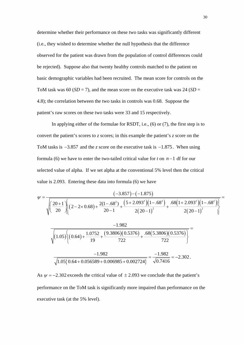
30

determine whether their performance on these two tasks was significantly different

(i.e., they wished to determine whether the null hypothesis that the difference

observed for the patient was drawn from the population of control differences could

be rejected). Suppose also that twenty healthy controls matched to the patient on

basic demographic variables had been recruited. The mean score for controls on the

ToM task was 60 (SD = 7), and the mean score on the executive task was 24 (SD =

4.8); the correlation between the two tasks in controls was 0.68. Suppose the

patient’s raw scores on these two tasks were 33 and 15 respectively.

In applying either of the formulae for RSDT, i.e., (6) or (7), the first step is to

convert the patient’s scores to z scores; in this example the patient’s z score on the

ToM tasks is and the z score on the executive task is 3.857− 1.875− . When using

formula (6) we have to enter the two-tailed critical value for t on 1n− df for our

selected value of alpha. If we set alpha at the conventional 5% level then the critical

value is 2.093. Entering these data into formula (6) we have

( ) ( )

( ) ( )( )( )

( )( )( )

2 2 2 22

2 2

3.857 1.875

5 2.093 1 .68 .68 1 2.093 1 .6820 1 2(1 .68 )2 2 0.6820 20 1 2 20 1 2 20 1

ψ− − −

= =⎧ ⎫+ − + −+ −⎪ ⎪⎛ ⎞ − × + + +⎨ ⎬⎜ ⎟ −⎝ ⎠ − −⎪ ⎪⎩ ⎭

( ) ( ) ( )( ) ( )( )1.982

9.3806 0.5376 .68 5.3806 0.53761.07521.05 0.6419 722 722

−=

⎧ ⎫+ + +⎨ ⎬

⎩ ⎭

{ }

1.982 1.982 2.3020.74161.05 0.64 0.056589 0.006985 0.002724

− −= = −

+ + +.

As 2.302ψ = − exceeds the critical value of ± 2.093 we conclude that the patient’s

performance on the ToM task is significantly more impaired than performance on the

executive task (at the 5% level).

31

As noted, formula (7) permits researchers to obtain a precise probability for

the difference between patient and controls and thereby also provides a point estimate

of the abnormality of the patient’s difference. Entering the data from the current

example into (7)

2(1 0.68)(1 0.68 ) 0.90317a = + − =

{ }2(1 0.68) 4(20 1) 4(1 0.68)(20 1) (1 0.68)(5 0.68) 505.99b = − − + + − + + + =

( ) ( ) ( )22 20 20 1

2 3.857 1.875 2701.1920 1

c⎛ ⎞−

= − − − − = −⎡ ⎤ ⎜ ⎟⎣ ⎦ ⎜ ⎟+⎝ ⎠

and therefore

( )( )

( )

1/ 22505.99 505.99 4 0.90317 2701.19

2.3002 0.90317

y⎛ ⎞− + − −⎜ ⎟= =⎜ ⎟⎝ ⎠

The two-tailed p value for a t of 2.30 on 19 df is 0.033 and therefore we come to the

same conclusion as that reached when we using formula (6); the patient’s ToM

performance is significantly more impaired (p < .05) than her/his performance on the

executive task. To obtain a point estimate of the abnormality of the patient’s

difference we use the one-tailed p value for t. The p value is 0.0165 and therefore we

estimate that only 1.65% of the control population would exhibit a discrepancy in

favour of the executive task of this magnitude and direction.

We can also use this example to illustrate the application of the revised criteria

for dissociations (see Table 5). Application of Crawford and Howell’s (1998) test (1)

reveals that the patient is significantly different (one-tailed) from controls on the ToM

task (t = 3.76, p = .001) and on the executive task (t = 1.83, p = .042). The patient is

therefore considered to have an impairment on both tasks and does not meet the

criteria for a classical dissociation. However, the patient does meet the criteria for a

32

strong dissociation; performance on both tasks is impaired but the ToM deficit is

significantly greater (i.e., the ToM deficit is a differential deficit).

Finally, the RSDT provides a very flexible method of testing for dissociations

as its use need not be limited to cases where performance is quantified by simple test

scores (such as number of items correct). For example, a patient’s memory for

temporal order is typically assessed by computing the rank-order correlation between

the order reported by a patient and the actual order of presentation. Similarly, in

estimation tasks, such as distance, weight or time estimation, performance is

commonly assessed by the slope of the regression line relating an individual’s

estimates to the actual distances, weights, or elapsed times. Crawford, Garthwaite,

Howell and Venneri (2003b) and Crawford and Garthwaite (2004) have recently

developed methods that allow single-case researchers to test whether a patient is

significantly different from a control sample when performance is quantified by a

parametric or non-parametric correlation coefficient or slope.

These authors noted that Crawford et al’s. (1998) test could be used to test

whether there was a dissociation between constructs measured by slopes or

correlations, or dissociations between such constructs and constructs measured by

conventional means. The present results suggest that the RSDT should be used for

this purpose instead. For example, it could be used to test if a patient exhibits a

dissociation between temporal order memory for verbal material and free recall of

such material; details of the treatment of patient and control data that are in the form

of slopes or correlations can be found in the aforementioned papers (Crawford &

Garthwaite, 2004; Crawford et al., 2003b).

33

Computer program to implement the revised difference tests and revised criteria for

dissociations

The calculations involved in applying the unstandardized difference test (5) or

RSDT (7) and thereby also obtaining a point estimate of the abnormality of the

patient's difference, could be performed by hand or calculator. However, the

calculations for the RSDT are tedious and prone to human error. For the foregoing

reasons we have implemented the statistical methods in a computer program

(dissocs.exe) for PCs.

The program prompts the user to select either the unstandardized difference

test or RSDT. The data inputs required are the means and SDs for Tasks X and Y and

the correlation between X and Y in controls, the N for the control sample, and the

patient's scores on X and Y. The results of applying the selected difference test are

reported, namely the t value and its associated two-tailed probability and the point

estimate of the abnormality of the patient's difference.

The program also applies the revised criteria for dissociations presented in the

present paper. That is, it applies Crawford and Howell's (1998) test to test for deficits

on Tasks X and Y (point estimates and confidence limits for the abnormality of the

patient’s scores are also reported), and uses these results together with the results of

the RSDT (or unstandardized difference test if the latter has been selected) to

establish whether the patient’s results fulfil the criteria for a classical or strong

dissociation. The results of these analyses can be viewed on screen, printed or saved

to a file. The program can be downloaded from the following web page address:

http://www.abdn.ac.uk/~psy086/dept/dissociations.htm.

34

Some comments and caveats on the use of single-case methods

The revised inferential methods for differences presented in the present paper

are both modified t-tests. As is the case for Crawford and Howell’s test, they assume

that the control sample data are normally distributed. Examining the robustness of

these tests in the face of skew is more complicated than was the case for the former

test as it is necessary to sample from skewed bivariate distributions and a larger

variety of scenarios need to be covered (e.g. investigating robustness when X and Y

are both skew, or only one of X and Y, studying effects of skew in opposite directions

for X and Y etc). However, we have conducted some provisional analysis of this issue

for the RSDT and obtained results that are as encouraging as those reported in Study

2 for Crawford and Howell’s test (Garthwaite & Crawford, in press). Nevertheless,

the results from applying these tests should be treated cautiously when the data

exhibit severe skew unless the resultant p value is well beyond .05 (i.e., < 0.025).

Importantly, the more commonly used alternative methods, e.g., the use of Dz or

Crawford et al’s. (1998) method to test for a difference between tasks, make exactly

the same assumption and will be equally compromised when this assumption is

violated.

The emphasis in the present paper has been on evaluating the performance of

the inferential tests for deficits and dissociations when single-case research is

conducted with modestly sized control samples. To avoid any potential confusion it

should be noted that the methods can be used with control samples of any size and

remain more valid than commonly used alternatives based on z when N is large; in

this situation the researcher is still dealing with a sample not a population.

Furthermore, although the methods achieve good control of Type I errors at small Ns,

this does not mean that researchers should limit themselves to recruiting small control

35

samples; the present paper focuses on small Ns simply because of the need to reflect

the reality of current practice in many single-case studies. Indeed, as noted, statistical

power is inevitably low in single-case studies (significant results are obtained because

effects are often large enough to overcome this). Therefore, it makes sense to

increase power by recruiting a large sample of controls when this is practical.

It should also be noted that very useful and elegant methods have been

devised for drawing inferences concerning an individual patient’s performance on

fully standardized neuropsychological tests; i.e., on tests that have been normed on

very large, representative samples of the population (e.g., Capitani, 1997; Capitani &

Laiacona, 2000; De Renzi, Faglioni, Grossi, & Nicheli, 1997; Willmes, 1985). When

these methods are used in single-case research, the patient is compared against

normative values rather than against controls. In such approaches, error arising from

sampling from the control population are ignored; this is justifiable because the

samples are large enough for such error to be minimal.

Although these latter approaches have much to commend them, unfortunately

they can be used only in fairly circumscribed situations because (a) the questions

posed in many single-case studies cannot be fully addressed using existing

standardized neuropsychological tests, (b) new constructs are constantly emerging in

neuropsychology, and (c) the collection of large-scale normative data is a

time-consuming and arduous process (Crawford, 2004). Therefore, there is a

continued need for methods that can be used when a patient is compared to a

modestly-sized control sample.

At the other extreme, some single-case studies do not refer the patient’s

performance to either a control sample or a large normative sample. That is,

conclusions on the presence of deficits and dissociations are based on intra-individual

36

analysis. An example of this approach comes from the aforementioned literature on

category-specificity. It is quite common for conclusions of a dissociation between

naming of living and non-living things to be based on a significant result from a

chi-square test; that is, a patient is administered an equal number of living and

non-living items and the number correctly named in each category is compared

(Laws, in press).

However, aside from the fact that the independence assumption for a

chi-square test is violated in these circumstances, there are further difficulties with

this approach. For example, Laws et al. (in press) studied AD patients who exhibited

significant differences (on chi-square tests) between the number of living and

non-living items named and found that many of these raw differences were not

unusual when standardized against control performance; i.e., the intra-individual

method yielded false positive indications of a dissociation. The opposite pattern was

also found; patients whose chi-square results were not significant showed strong

evidence of a dissociation when their naming was referenced to control performance.

The focus of the present study has been on inferential methods for single tests

(when attempting to detect deficits) or pairs of tests (when attempting to detect

dissociations). However, it should be acknowledged that findings obtained from

comparing the patient to a control sample are not interpreted in isolation. Rather,

these findings are interpreted in the context of results from a prior assessment in

which a broad characterisation of the patient’s strengths and weaknesses will have

been achieved through the use of fully or partially standardized tests.

Furthermore, many single-case studies employ multiple measures of the

constructs under investigation (i.e., different but related tasks X1, X2 etc and Y1, Y2 etc

to measure constructs X and Y). That is, the patient is compared to controls over a

37

series of tasks. This is in keeping with the fact that researchers are ultimately

interested in dissociations between functions, not just in dissociations between

specific pairs of indirect and imperfect measures of these functions (Crawford et al.,

2003b; Vallar, 2000). Thus, researchers seek converging evidence of a deficit or

dissociation (Vallar, 2000). The upshot of this is that the risk of drawing incorrect

conclusions will typically be less than that associated with the results from a single

inferential test (in the case of a deficit) or single application of a set of criteria (in the

case of a dissociation).

However, the integration of these multiple sources of information is a complex

and formidable task. It is fair to say that (a) currently there is little consistency across

studies in how this task is approached, and (b) existing attempts tend to be qualitative

rather than quantitative. The development of a quantitative system, whereby the

probabilities (e.g., of a dissociation) could be combined or updated as different stages

of a study are completed, would make a very significant contribution to the discipline.

The nature of this problem is such that an approach based on Bayesian rather than

classical (i.e., frequentist) methods would be the obvious choice.

Finally, a central aim of the present study was to develop and evaluate more

rigorous criteria for dissociations than those employed previously. However, even if

infallible criteria for identifying dissociations were available, there remains the wider

and thornier issue of what dissociations allow us to conclude about the functional

architecture of human cognition. Although this is a large topic, and one that lies

beyond the scope of the present study, a few comments are in order.

It is generally acknowledged that a single dissociation implies that different

cognitive functions underlie performance on the two tasks in question, but that such

dissociations are prone to task difficulty artefacts. That is, a unitary cognitive

38

function may contribute to performance on both tasks X and Y, but only task X is of

sufficient difficulty to uncover an impairment of this function (Crawford et al., 2003a;

Vallar, 2000). The identification of a double dissociation (i.e., patients who have

opposite patterns of spared and impaired performance) is generally considered to

largely rule out such artefacts. For this reason the double dissociation is a central tool

for the building and testing of theory in neuropsychology. As Vallar (2000) notes, the

double dissociation provides “…the most effective paradigm for investigating the

modularity of the mental processes and their neural correlates” (p. 329). However,

serious areas of debate remain (Dunn & Kirsner, 2003; Shallice, 1988). For example,

Dunn and Kirsner (2003) argue that, (a) we can only specify the characteristics of

cognitive modules underlying a double dissociation if the cases involved are pure

cases and the tasks are process pure, and (b) there is no independent means of testing

whether (a) holds. Thus their pessimistic conclusion is that “dissociations may tell us

nothing more about mental functions other than that there are two of them” (p. 5).

Conclusion

The single-case approach in neuropsychology has made a significant

contribution to our understanding of the functional architecture of human cognition.

However, as Caramazza and McCloskey (1988) note, if advances in theory are to be

sustainable they “… must be based on unimpeachable methodological foundations”

(p. 619). The statistical treatment of single-case study data is one area of

methodology that has been relatively neglected. In the present paper the evaluation of

inferential tests for comparing a patient to a control sample provides researchers with

simulation results to guide their choice of methods and provides new methods that

have significant advantages over the existing alternatives.

39

40

References

Baron-Cohen, S., Leslie, A. M., & Frith, U. (1985). Does the autistic child

have a theory of mind. Cognition, 21, 37-46.

Boneau, C. A. (1960). The effect of violation of assumptions underlying the t-

test. Psychological Bulletin, 57, 49-64.

Box, G. E. P., & Muller, M. E. (1958). A note on the generation of random

normal deviates. Annals of Mathematical Statistics, 28, 610-611.

Capitani, E. (1997). Normative data and neuropsychological assessment.

Common problems in clinical practice and research. Neuropsychological

Rehabilitation, 7(295-309).

Capitani, E., & Laiacona, M. (2000). Classification and modelling in

neuropsychology: from groups to single cases. In F. Boller & J. Grafman (Eds.),

Handbook of neuropsychology (2nd ed., Vol. 1, pp. 53-76). Amsterdam: Elsevier.

Caramazza, A., & McCloskey, M. (1988). The case for single-patient studies.

Cognitive Neuropsychology, 5, 517-528.

Coltheart, M. (2001). Assumptions and methods in cognitive

neuropsychology. In B. Rapp (Ed.), The handbook of cognitive neuropsychology (pp.

3-21). Philadelphia: Psychology Press.

Crawford, J. R. (2004). Psychometric foundations of neuropsychological

assessment. In L. H. Goldstein & J. E. McNeil (Eds.), Clinical neuropsychology: A

practical guide to assessment and management for clinicians (pp. 121-140).

Chichester: Wiley.

Crawford, J. R., & Garthwaite, P. H. (2002). Investigation of the single case in

neuropsychology: Confidence limits on the abnormality of test scores and test score

differences. Neuropsychologia, 40, 1196-1208.

41

Crawford, J. R., & Garthwaite, P. H. (2004). Statistical methods for single-

case research: Comparing the slope of a patient's regression line with those of a

control sample. Cortex, in press.

Crawford, J. R., Garthwaite, P. H., & Gray, C. D. (2003a). Wanted: Fully

operational definitions of dissociations in single-case studies. Cortex, 39, 357-370.

Crawford, J. R., Garthwaite, P. H., Howell, D. C., & Gray, C. D. (in press).

Inferential methods for comparing a single case with a control sample: Modified t-

tests versus Mycroft et al's. (2002) modified ANOVA. Cognitive Neuropsychology.

Crawford, J. R., Garthwaite, P. H., Howell, D. C., & Venneri, A. (2003b).

Intra-individual measures of association in neuropsychology: Inferential methods for

comparing a single case with a control or normative sample. Journal of the

International Neuropsychological Society, 9, 989-1000.

Crawford, J. R., Howell, D. C., & Garthwaite, P. H. (1998). Payne and Jones

revisited: Estimating the abnormality of test score differences using a modified paired

samples t-test. Journal of Clinical and Experimental Neuropsychology, 20, 898-905.

Crawford, J. R., & Howell, D. C. (1998). Comparing an individual’s test score

against norms derived from small samples. The Clinical Neuropsychologist, 12, 482-

486.

De Renzi, E., Faglioni, P., Grossi, D., & Nicheli, P. (1997). Apperceptive and

associative forms of prosopagnosia. Cortex, 27, 213-221.

Dunn, J. C., & Kirsner, K. (2003). What can we infer from double

dissociations? Cortex, 39, in press.

Ellis, A. W., & Young, A. W. (1996). Human cognitive neuropsychology: A

textbook with readings. Hove, UK: Psychology Press.

42

Garthwaite, P. H., & Crawford, J. R. (in press). The distribution of the

difference between two t-variates. Biometrika.

Garvin, J. S., & McClean, S. I. (1997). Convolution and samling theory of the

binormal distribution as a prerequisite to its application in statistical process control.

The Statistician, 46, 33-47.

Gibbons, J. F., & Mylroie, S. (1973). Estimation of impurity profiles in ion-

implanted amorphous targets using half-Gaussian distributions. Applied Physics

Letters, 22, 568-569.

Howell, D. C. (2002). Statistical methods for psychology (5th ed.). Belmont,

CA: Duxbury Press.

Kennedy, W. J., & Gentle, J. E. (1980). Statistical computing. New York:

Marcel Dekker.

Kimber, A. C. (1985). Methods for the two-piece normal distribution.

Communications in Statistics-Theory and Methods, 14, 235-245.

Laws, K. R. (in press). Illusions of normality: A methodological critique of

category-specific naming. Cortex.

Laws, K. R., Gale, T. M., Leeson, V. C., & Crawford, J. R. (in press). When is

category specific in Alzheimer's disease? Cortex.

Payne, R. W., & Jones, G. (1957). Statistics for the investigation of individual

cases. Journal of Clinical Psychology, 13, 115-121.

Press, W. H., Flannery, B. P., Teukolsky, S. A., & Vetterling, W. T. (1989).

Numerical recipes in Pascal. Cambridge: Cambridge University Press.

Shallice, T. (1979). Case study approach in neuropsychological research.

Journal of Clinical Neuropsychology, 3, 183-211.

43

Shallice, T. (1988). From neuropsychology to mental structure. Cambridge,

UK: Cambridge University Press.

Siddiqui, M. M. (1967). A bivariate t-distribution. Annals of Mathematical

Statistics, 38, 162-166.

Sokal, R. R., & Rohlf, J. F. (1995). Biometry (3rd ed.). San Francisco, CA:

W.H. Freeman.

Vallar, G. (2000). The methodological foundations of human

neuropsychology: studies in brain-damaged patients. In F. Boller & J. Grafman

(Eds.), Handbook of neuropsychology (2nd ed., Vol. 1, pp. 53-76). Amsterdam:

Elsevier.

Willmes, K. (1985). An approach to analyzing a single subject's scores

obtained in a standardized test with application to the Aachen Aphasia Test (AAT).

Journal of Clinical and Experimental Neuropsychology, 7, 331-352.

44

Table 1. Results from a Monte Carlo simulation study of the percentage of control

cases classified as exhibiting a deficit (i.e. percentage of Type I errors) using z and a

modified t-test when the specified error rate is 5%

Percentage of Type I errors

Control sample N z t z required*

5 10.37 5.01 -2.335

10 7.57 5.00 -1.923

20 6.25 5.00 -1.772

50 5.53 5.03 -1.693

100 5.28 4.98 -1.669

*Records the value of z required to maintain the Type I error rate at the specified (5%) level

Analysis of Single Case 45

Table 2. Simulation results: percentage of Type I errors (i.e. percentage of control cases classified as exhibiting a deficit) using z and a modified t-test for

a specified error rate of 5% when sampling from (negatively) skewed distributions

Moderate skew ( )1 0.31g = − Severe ( 1 0.70g = − ) Very severe ( 1 0.93g = − ) Extreme ( 1 0.99g = − )

N Z t z t z t z t

5

11.48 6.06 12.50 7.23 13.23 8.04 13.39 8.27

10 8.59 6.04 9.64 7.14 10.23 7.80 10.23 7.94

20 7.23 5.97 8.20 6.97 8.72 7.53 8.72 7.66

50 6.50 6.00 7.37 6.90 7.85 7.37 7.85 7.47

100 6.20 5.97 7.11 6.87 7.56 7.32 7.56 7.32

Analysis of Single Case 46

Table 3. Simulation results: percentage of control cases exhibiting significant differences between tasks X and Y (i.e., percentage of Type I errors) when

using three inferential tests under different values of N of the control sample and correlations between tasks

Payne & Jones (1957) test ( Dz ) Crawford et al’s (1998) test ( ) Dt Unstandardized difference test ( ) UDt

N 0.0 0.2 0.5 0.8 0.0 0.2 0.5 0.8 0.0 0.2 0.5 0.8

5

21.02 22.05 23.78 25.70 9.18 9.91 10.97 12.31 5.00 5.01 5.01 5.04

10 11.57 11.94 12.58 13.18 6.55 6.82 7.31 7.75 5.01 4.98 5.04 5.03

20 7.91 8.05 8.30 8.59 5.66 5.77 6.00 6.23 4.99 4.99 5.01 5.03

50 6.09 6.11 6.21 6.28 5.27 5.26 5.36 5.43 5.03 4.96 5.01 5.00

100 5.53 5.55 5.59 5.60 5.12 5.15 5.18 5.19 5.00 5.02 5.00 4.97

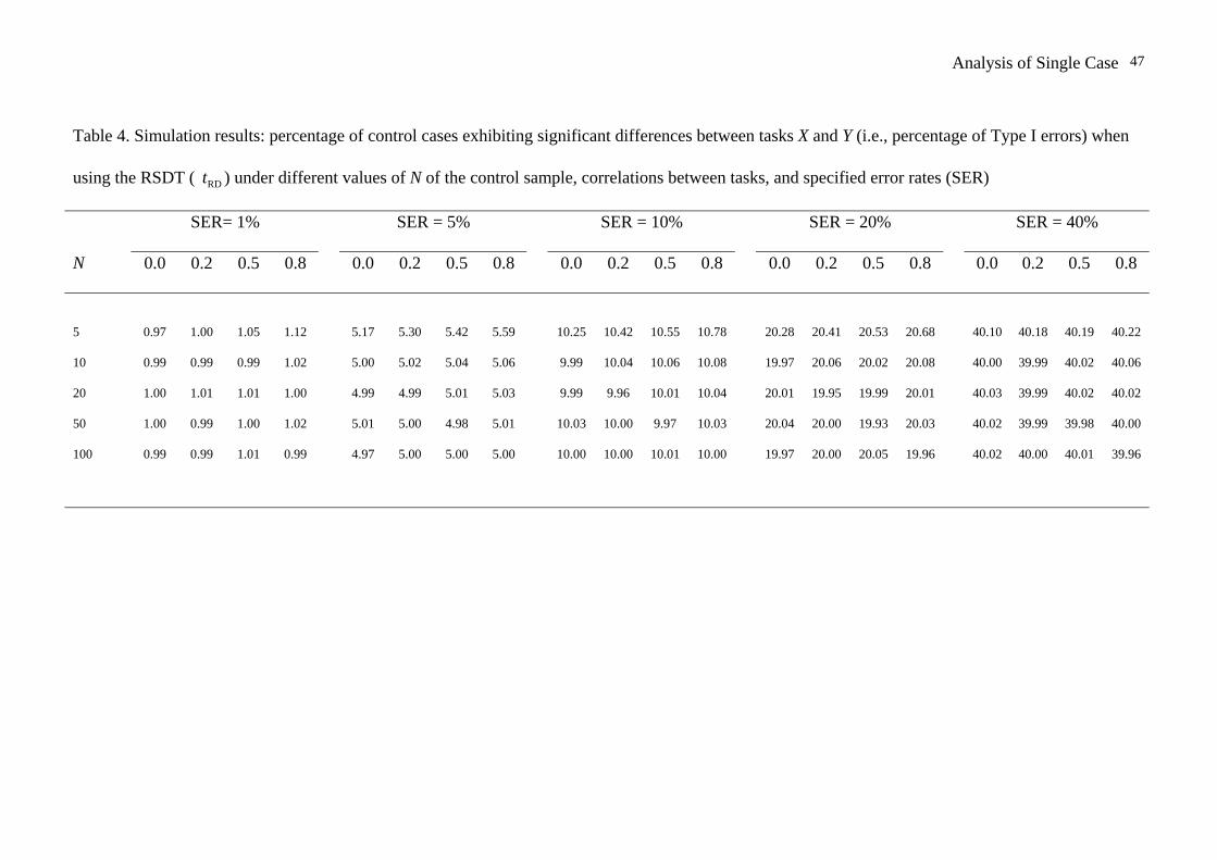
Analysis of Single Case 47

Table 4. Simulation results: percentage of control cases exhibiting significant differences between tasks X and Y (i.e., percentage of Type I errors) when

using the RSDT ( ) under different values of N of the control sample, correlations between tasks, and specified error rates (SER) RDt

SER= 1% SER = 5% SER = 10% SER = 20% SER = 40%

N 0.0 0.2 0.5 0.8 0.0 0.2 0.5 0.8 0.0 0.2 0.5 0.8 0.0 0.2 0.5 0.8 0.0 0.2 0.5 0.8

5

0.97 1.00 1.05 1.12 5.17 5.30 5.42 5.59 10.25 10.42 10.55 10.78 20.28 20.41 20.53 20.68 40.10 40.18 40.19 40.22

10 0.99 0.99 0.99 1.02 5.00 5.02 5.04 5.06 9.99 10.04 10.06 10.08 19.97 20.06 20.02 20.08 40.00 39.99 40.02 40.06

20 1.00 1.01 1.01 1.00 4.99 4.99 5.01 5.03 9.99 9.96 10.01 10.04 20.01 19.95 19.99 20.01 40.03 39.99 40.02 40.02

50 1.00 0.99 1.00 1.02 5.01 5.00 4.98 5.01 10.03 10.00 9.97 10.03 20.04 20.00 19.93 20.03 40.02 39.99 39.98 40.00

100 0.99 0.99 1.01 0.99 4.97 5.00 5.00 5.00 10.00 10.00 10.01 10.00 19.97 20.00 20.05 19.96 40.02 40.00 40.01 39.96

Analysis of Single Case 48Table 5. Revised criteria for classical and strong dissociations obtained by modifying

Crawford, Garthwaite and Gray’s (2003) original criteria

Dissociation Criteria

Classical Dissociation 1) Patient’s score on Task X significantly lower than controls (p < 0.05, one-tailed) on Crawford & Howell’s (1998) test; i.e., score meets the criterion for an impairment

2) Patient’s score on Task Y not significantly lower than controls (p > 0.05, one-tailed) on Crawford & Howell’s test; i.e., score fails to meet criterion for an impairment and is therefore considered to be within normal limits

3) Patient’s score on Task X significantly lower (p < .05; two-tailed) than patient’s score on Task Y using the RSDT. The test is two-tailed to allow for the fact that the data are examined before deciding which task is X and which is Y

Strong Dissociation (i.e., differential deficit)

1) Patient’s score on Task X significantly lower than controls (p < 0.05, one-tailed) on Crawford & Howell’s (1998) test; i.e., score meets the criterion for an impairment

2) Patient’s score on Task Y is also significantly lower than controls (p < 0.05, one-tailed) on Crawford & Howell’s (1998) test; i.e., score meets the criterion for an impairment

3) Patient’s score on Task X significantly lower (p < .05, two-tailed) than patient’s score on Task Y using the RSDT.

Classical Double dissociation

1) Patient 1 meets the criterion for a deficit on Task X, and meets the criteria for a classical dissociation between this task and Task Y.

2) Patient 2 meets the criterion for a deficit on Task Y and meets the criteria for a classical dissociation between this task and Task X.

Strong Double Dissociation

1) Patient 1 meets the criterion for a deficit on Task X, and meets the criteria for a classical or strong dissociation between this task and Task Y.

2) Patient 2 meets the criterion for a deficit on Task Y and meets the criteria for a classical or strong dissociation between this task and Task X.

3) Only one of the above dissociations are classical (otherwise we have a classical double dissociation).

Analysis of Single Case 49

Table 6. Results from a Monte Carlo simulation study: percentage of control cases incorrectly classified as exhibiting strong and classical dissociations when is used to test for

differences between tasks X and Y under different values of N of the control sample and correlations between tasks

RDt

Strong Dissociation Classical Dissociation

N 0.0 0.2 0.5 0.8 0.0 0.2 0.5 0.8

5

0.01 0.02 0.07 0.22 2.32 2.03 1.64 1.12

10 0.00 0.01 0.03 0.12 2.41 2.06 1.56 0.98

20 0.00 0.00 0.01 0.07 2.48 2.06 1.50 0.90

50 0.00 0.00 0.01 0.04 2.51 2.06 1.49 0.84

100 0.00 0.00 0.00 0.04 2.49 2.10 1.48 0.84

Analysis of Single Case 50Figure Legends

Figure 1.

Graphical illustration of the four negatively skewed distributions employed in Study 2

Figure 2.

Monte Carlo simulation results: Type I errors for three tests on the difference between a

patient’s scores on two tasks (results are for a XYρ of 0.5)

Analysis of Single Case 51

(a) Moderate skew (g1 = -0.31)

(b) Severe skew (g1 = -0.70)

(c) Very severe skew (g1 = -0.93) (d) Extreme skew (g1 = -0.99)

Analysis of Single Case 52

0

5

10

15

20

25

5 10 20 50 100

Control sample size

Perc

enta

ge T

ype

I err

ors

P&JCH&GRSDT