testing informational efficiency: the case of u.e. and...

Studies in Business and Economics

- 94 - Studies in Business and Economics

TESTING INFORMATIONAL EFFICIENCY: THE CASE OF

U.E. AND BRIC EMERGENT MARKETS

OPREAN Camelia

Lucian Blaga University of Sibiu, Romania

Abstract:

Empirical finance has brought together a considerable number of studies in determining

the market efficiency in terms of information in the case of an emerging financial market.

Conflicting results have been generated by these researches in efficient market hypothesis

(EMH), so efficiency tests in the emerging financial markets are rarely definitive in reaching a

conclusion about the existence of informational efficiency. This paper tests weak-form market

efficiency of eight emerging markets: four U.E emerging markets: Romania, Hungary, Czech

Republic, Slovakia, Estonia and BRIC emerging markets: Brazil, Russia, India and China. The

random walk hypothesis of stock exchange indices is tested using statistical tests. To test for the

existence of the normality hypothesis of distributed instantaneous yields (logarithmic) of stock

index are employed Jarque-Bera and QQ-plot tests. The stationary tests for instantaneous yields

(logarithmic) of stock exchange indexed that are used in this article are unit root tests, run tests

and variance ratio test. Because the analysis determined empirically the presence of linear

dependences for the returns series, it can be concluded that most of these emerging equity

markets are not weak-form efficient.

Key words: efficient market hypothesis, information, tests, emergent, random walk

1. Introduction

There are two main theories that considerations concerning the efficiency of

financial markets lay under: the theory of efficient markets and the random walk theory.

In his famous study, which will definitively mark the theory of efficient markets, Efficient

Capital Markets: A Review of Theory and Empirical Work, written by Fama in 1970, he

gives the following definition: “A market in which prices always reflect the available

information is called an efficient market”. The market efficiency hypothesis (EMH) is

a statement about:

the theory that stock prices reflect the true value of stocks;


Studies in Business and Economics - 95 -

the absence of arbitrage opportunities in an economy populated by rational,

profit-maximizing agents;

the hypothesis that market prices always fully reflect available information

(Fama 1970).

Therefore the rational expectations of the returns for a particular stock

according to the EMH may be represented as:

111 ε +++ += tttt PEP

where tP is the stock price; and 1t is the forecast error. 11 ttt PEP should therefore

be zero on average and should be uncorrelated with any information t . Also

0)|( 1, ttjxE when the random variable (good or bad news), the expected value

of the forecast error, is zero:

0)( 11111 tttttttttt PEPEPEPEE

The Random Walk Model (RWM) is the model which assumes that

subsequent price changes are sovereign and homogeneously distributed random

variables and concludes that changes in assets prices cannot be forecasted through

historical price changes and movements. The Random Walk Model is generally used

to test the weak-form Efficient Market Hypothesis (Hamid K. et all, 2010).

Random walk theory claims that stock market can be analyzed as random walk

according to the next three facts (Vulic, 2010):

efficient markets respond very fast to new information;

if the share price is a reflection of all available information, it is impossible to

use that information for market predictions;

it is impossible to predict market movement other than randomly.

The empirical evidences show that the random walk hypothesis is “almost

approximately true”. More precisely, if the financial assets returns are partial

predictable, both on the short time, and on the medium and long time, the degree of

predictability is generally low comparative with the high volatility of these returns.

A random walk is a usual example of a non-stationary series:

where εt is a casual perturbation with stationary character. The series yt present an

upward variance in time, while its 1st difference is stationary because:

Emerging equity markets are widely thought to be places of substantial trading

profits and weak and semi-strong form market inefficiencies when compared to

developed markets. In their article, Griffin, Kelly and Nardari, 2009, examine the extent

to which this is true using a variety of methodologies and data from 28 developed and

28 emerging markets. Emerging markets exhibit similar autocorrelation in firm returns,

suggesting that they are not under or overreacting to news contained in past returns

any more than in developed markets. Emerging markets incorporate past market and

portfolio returns into prices slightly better than developed markets.



Using the article of Basu and Morey (2005), who developed a theoretical

model that explores the effect of trade openness on stock return autocorrelation

patterns, the paper of Lim and Kim, 2008, brings their proposition to the data,

examining the impact of liberalization policies, both trade and financial, on the

informational efficiency of 23 emerging stock markets. In general, the key results from

fixed effects panel regressions support their prediction that trade liberalization, rather

than financial openness, matters the most for informational efficiency.

Islam, Watanapalachaikul, Clark (2007) proposed a theory-free paradigm of

non-parametric tests of market efficiency for an emerging stock market, the Thai stock

market, consisting of two tests which are run-test and autocorrelation function tests

(ACF), to establish a more definitive conclusion about EMH in emerging financial

markets. The result of this research demonstrates that an autocorrelation on Thai stock

market returns exists particularly during the post-crisis period.

Regarding Romanian capital market, it has been investigated rationality of

Romanian investors, and efficiency market hypothesis represented a useful tool in

order to achieve this goal (Dragotă, Mitrica, 2004). The tests suggested by Fama

[1970] have been successfully applied by many authors. Therefore, for many

Romanian researchers it was incentive to proceed on investigating informational

efficiency of Romanian capital market. Most of these studies have focused on the weak

form of informational market efficiency using in that sense autocorrelation coefficients,

normality and stationarity tests (Augmented Dickey-Fuller and Phillips-Perron) in order

to test random walk pattern for stock returns.

Lazăr and Ureche (2007) tested weak-form market efficiency of eight emerging

markets: Romania, Hungary, Czech Republic, Lithuania, Poland, Slovakia, Slovenia,

Turkey. The used tests determined empirically the presence of linear and nonlinear

dependences, for most of the returns series. Most of these emerging equity markets

were not weak-form efficient.

This paper is structured as follows: section 2 presents the data and empirical

methodology used for testing the weak-form of informational efficiency of the eight

emerging capital markets. The empirical results of these tests are presented in section

3. The conclusions are given in the last section 4.

2. Data and methodology

The data used for this study is the market value-weighted equity indices (BET

for Romania, SAX Index for Slovakia, OMX Tallinn for Estonia, PX for Czech Republic,

BUX for Hungary, IBOVESPA for Brazil, RTSI for Russia, SENSEX for India and

Shanghai Composite Index for China). In the past years, the stock markets have

witnessed heightened activity in terms of various bull and bear runs. The reason for

which we used in our study the stock markets indices is that usually the indices have

the ability to capture all these happenings on the markets in the most judicious

manner. One can identify the booms and busts of the equity markets through indices.

Their brief description is given in table 1:



Table 1 – Description of the emergent stock exchange indices

Index Description

BET Index –

Bucharest Stock

Exchange

the first index developed by BVB, is the reference index for the BVB

market. BET is a free float weighted capitalization index of the most liquid

10 companies listed on the BVB regulated market. The index

methodology allows BET to be a good underlying for derivatives and

structured products.

PX Index – Prague

Stock Exchange

the official index of the Prague Stock Exchange. It is a capitalization

weighted price index and is made up of the most traded blue chips at the

Stock Exchange. It is designed as a tradable index to be used as an

underlying asset for structured products and for standardized derivatives

(future).

OMX Tallinn Index –

Tallinn Stock

Exchange

an all-share index which includes all the shares listed on the Main and

Secondary lists on the NASDAQ OMX Tallinn (the Tallinn Stock

Exchange is the only regulated exchange in Estonia) with exception of

the shares of the companies where a single shareholder controls at least

90% of the outstanding shares.

BUX Index –

Budapest Stock

Exchange

the official index of blue-chip shares listed on the Budapest Stock

Exchange Ltd. The index shows the average price changing of the shares

with the biggest market value and turnover in the equity section.

Bovespa Index –

BM&FBOVESPA

Stock Exchange

the main indicator of the Brazilian stock market’s average performance.

Ibovespa’s relevance comes from two facts: it reflects the variation of

BM&FBOVESPA’s most traded stocks and it has tradition, having

maintained the integrity of its historical series without any methodological

change since its inception in 1968.

RTS Index –

"Russian Trading

System" Stock

Exchange

the composite index of the Russian stock market calculated by Moscow

Interbank Currency Exchange (“ZAO MICEX”).

SENSEX Index –

Bombay Stock

Exchange

first compiled in 1986, was calculated on a "Market Capitalization-

Weighted" methodology of 30 component stocks representing large, well-

established and financially sound companies across key sectors. Since

September 1, 2003, SENSEX is being calculated on a free-float market

capitalization methodology. As the oldest index in the country, it provides

the time series data over a fairly long period of time (from 1979 onwards).

SSE Composite

Index – Shanghai

Stock Exchange

was launched on July 15, 1991. Constituents are all listed stocks (A

shares and B shares) at Shanghai Stock Exchange.The Base Day for

SSE Composite Index is December 19, 1990. The Base period is the total

market capitalization of all stocks of that day.

The time series cover a period of 10 years, from october 2002 to october 2012.

The data consist of around 2500 daily values of every index. The returns have been

measured using the first difference of monthly logarithmic price index:

)(log)(log)(log 1 tetetet CCCdR



Our empiric test followed the research of the random walk hypothesis of every

index, using the following tests:

Tests looking for the existance of the normality hypothesis of distributed

instantaneous returns (logarithmic) of stock indices: we use the graphical

analysis, Jarque-Bera test and QQ-plot test;

Stationary tests for instantaneous returns (logarithmic) of stock indices:

unit root tests (Augmented Dickey-Fulle test, Phillips-Perron test,

autocorrelation coefficients and Ljung-Box test), run test and variance ratio

test.

3. Empirical results

I. Tests on the hypothesis of normality of instantaneous returns of indices

In order to test the normality distribution hypothesis of the logarithmic (or

continuously compounded) returns of indices it is used the Jarque-Bera test and QQ-

plot test.

To study the normality, there are used the following indicators: Kurtosis,

Skewness and Jarque-Bera.

The Jarque–Bera test is a test of whether sample data of returns have the

skewness and kurtosis matching a normal distribution. Samples from a normal

distribution have an expected skewness of 0 and an expected excess kurtosis of 0

(which is the same as a kurtosis of 3). As the definition of JB shows, any deviation from

this increases the JB statistic. If kurtosis is bigger than 3, the distribution is called

leptokurtotic and if it is less than 3, platykurtotic.

Also, to test the hypothesis of normality of instantaneous returns of indices, we

used QQ-plot test. Theoretical quantile-quantile plots are used to assess whether the

data in a single series follow a specified theoretical distribution. If the two distributions

are the same, the QQ-plot should lie on a straight line. If the QQ-plot does not lie on a

straight line, the two distributions differ along some dimension. The pattern of deviation

from linearity provides an indication of the nature of the mismatch.

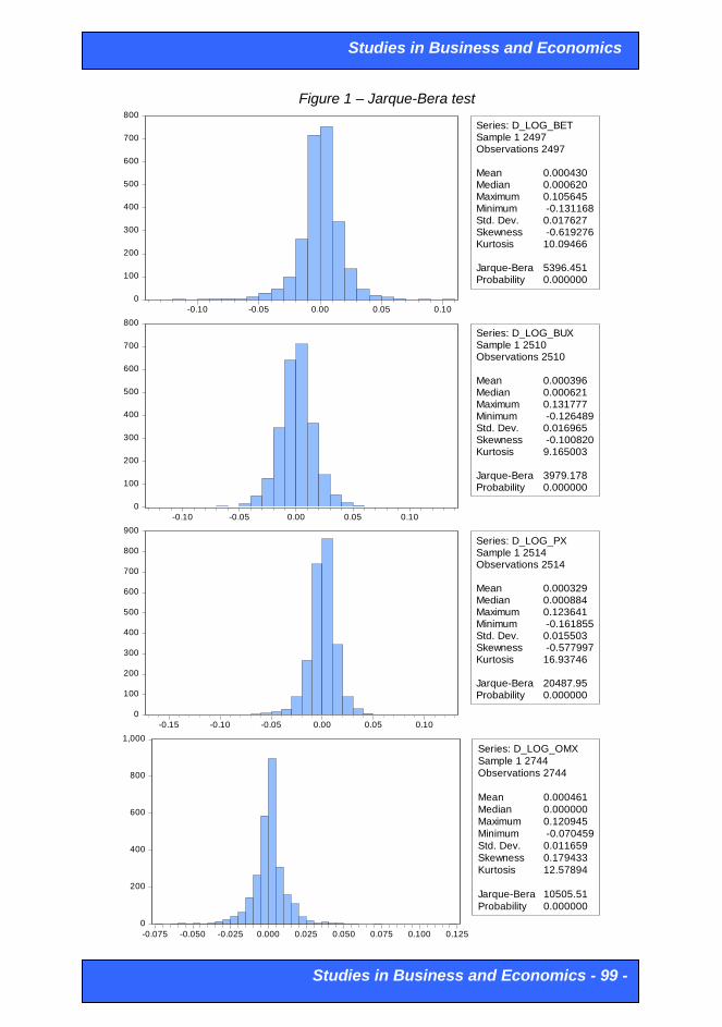
The graphics of the Jarque-Bera and QQ-plot tests for every index are

presented below:

http://en.wikipedia.org/wiki/Skewness

http://en.wikipedia.org/wiki/Kurtosis

http://en.wikipedia.org/wiki/Normal_distribution



Figure 1 – Jarque-Bera test

0

100

200

300

400

500

600

700

800

-0.10 -0.05 0.00 0.05 0.10

Series: D_LOG_BETSample 1 2497Observations 2497

Mean 0.000430Median 0.000620Maximum 0.105645Minimum -0.131168Std. Dev. 0.017627Skewness -0.619276Kurtosis 10.09466

Jarque-Bera 5396.451Probability 0.000000

0

100

200

300

400

500

600

700

800

-0.10 -0.05 0.00 0.05 0.10

Series: D_LOG_BUXSample 1 2510Observations 2510



0

100

200

300

400

500

600

700

800

900

-0.15 -0.10 -0.05 0.00 0.05 0.10

Series: D_LOG_PXSample 1 2514Observations 2514



0

200

400

600

800

1,000

-0.075 -0.050 -0.025 0.000 0.025 0.050 0.075 0.100 0.125

Series: D_LOG_OMX

Sample 1 2744

Observations 2744

Mean 0.000461

Median 0.000000

Maximum 0.120945

Minimum -0.070459

Std. Dev. 0.011659

Skewness 0.179433

Kurtosis 12.57894

Jarque-Bera 10505.51

Probability 0.000000



0

100

200

300

400

500

600

700

-0.10 -0.05 0.00 0.05 0.10

Series: DLOGIBOVESPASample 1 2476Observations 2476

Mean -0.000708Median -0.001355Maximum 0.120961Minimum -0.136766Std. Dev. 0.018534Skewness 0.098634Kurtosis 8.102144


0

200

400

600

800

1,000

1,200

1,400

-0.2 -0.1 0.0 0.1 0.2

Series: D_LOG_RTSI

Sample 1 2493

Observations 2493

Mean 0.000573

Median 0.002084

Maximum 0.202039

Minimum -0.211994

Std. Dev. 0.022475

Skewness -0.498767

Kurtosis 13.98378



0

100

200

300

400

500

600

700

800

-0.15 -0.10 -0.05 0.00 0.05 0.10

Series: D_LOG_SENSEXSample 1 2474Observations 2474

Mean -0.000764Median -0.001333

Maximum 0.118092Minimum -0.159900Std. Dev. 0.016421Skewness 0.085062Kurtosis 10.75246


0

100

200

300

400

500

-0.075 -0.050 -0.025 0.000 0.025 0.050 0.075

Series: D_LOG_SHANGHAI_C_I

Sample 1 2512

Observations 2512

Mean -0.000128

Median -8.35e-05

Maximum 0.092562

Minimum -0.090343

Std. Dev. 0.016584

Skewness 0.246220

Kurtosis 6.627945





Figure 2 – Quantile-Quantile plot

-.08

-.06

-.04

-.02

.00

.02

.04

.06

.08

-.15 -.10 -.05 .00 .05 .10 .15

Quantiles of DLOG(BET__LEI_)

Qu

an

tile

s o

f N

orm

al

-.08

-.06

-.04

-.02

.00

.02

.04

.06

.08

-.15 -.10 -.05 .00 .05 .10 .15

Quantiles of D_LOG_BUX

Qu

an

tile

s o

f N

orm

al

-.06

-.04

-.02

.00

.02

.04

.06

-.20 -.15 -.10 -.05 .00 .05 .10 .15

Quantiles of D_LOG_PX

Qu

an

tile

s o

f N

orm

al

-.06

-.04

-.02

.00

.02

.04

.06

-.08 -.04 .00 .04 .08 .12 .16

Quantiles of D_LOG_OMX

Qu

an

tile

s o

f N

orm

al

-.08

-.06

-.04

-.02

.00

.02

.04

.06

.08

-.15 -.10 -.05 .00 .05 .10 .15

Quantiles of D_LOG_IBOVESPA

Qu

an

tile

s o

f N

orm

al

-.100

-.075

-.050

-.025

.000

.025

.050

.075

.100

-.3 -.2 -.1 .0 .1 .2 .3

Quantiles of D_LOG_RTSI

Qu

an

tile

s o

f N

orm

al

-.06

-.04

-.02

.00

.02

.04

.06

-.20 -.15 -.10 -.05 .00 .05 .10 .15

Quantiles of D_LOG_SENSEX

Qu

an

tile

s o

f N

orm

al

-.06

-.04

-.02

.00

.02

.04

.06

-.100 -.075 -.050 -.025 .000 .025 .050 .075 .100

Quantiles of D_LOG_SHANGHAI_C_I

Qu

an

tile

s o

f N

orm

al



The main results from the upper histograms and QQ-plots are presented as

follows:

The lowest mean returns is observed in India, with a value of -0.076% and in

Brazil (-0.07%) and the highest mean returns are for the Russian index returns

(0.057%). The market risk measured using standard deviation is higher in Russia,

this capital market being characterised by a higher volatility and lower in Estonia.

A negative skewness shows that the lower deviations from the mean are larger

than the upper deviations, indicating a greater probability of large deceases than

rises. The BET, BUX, PX and RTSI series are asymmetric on the left, because the

Skewness indicator (the asymmetry coefficient) is negative. Also, the OMX,

IBOVESPA, SENSEX and Shanghai_C_I are asymmetric on the right, because

the Skewness indicator (the asymmetry coefficient) is positive. The Kurtosis

indicator (the flattening coefficient) shows us that the series have a vaulting

superior to the one specific to the normal distribution (k=3), the distribution of the

daily instantaneous returns of all the eight indices being leptokurtosis. If the

associated probability of the test is bigger than the chosen relevance level (1, 5,

10%), the null hypothesis of normal distribution is accepted. In our study, because

the value of the associated probability is zero, the null hypothesis of normal

distribution of indices is rejected.

As it can be noticed from the analyzed data, the QQ-plot charts for all the indices

highlight the fact that the daily yields are not normally distributed. Also, we cannot

conclude that the series distributions are normal based on the Jarque-Bera test.

Almost all markets exhibits significant deviations from normality. Because of the

correlation existing between yields, and because they do not have a normal

distribution, we reject the hypothesis that these time series are random walk type

and so, serious question marks are raised regarding the existence of weak form

informational efficiency on the these eight emergent capital markets.

The further analysis requires that whether the time series are non-stationary or

stationary.

II. Stationary tests for instantaneous returns of BET index

The stationary tests for instantaneous yields (logarithmic) of stock index used

are: unit root tests, run test and variance ratio test.

a. Unit root tests

To test the stationary for instantaneous returns, daily calculated, of the stock

indices we use Augmented Dickey-Fuller (ADF) and Phillips-Perron tests. Also, the

autocorrelation coefficients are calculated and the Ljung-Box test is used.

Augmented Dickey-Fuller is the most popular stationary test. It was

presented by the statisticians David Alan Dickey and Wayne Arthur Fuller in 1979 and



1981. ADF test is used to test the unit root hypothesis. If one time series has unit root

that means it is nonstationary and it follows random walk. ADF Test Statistic and PP

Test Statistic represent the t test for accepting or rejecting the null hypothesis of the

Dickey-Fuller and Phillips Perron tests. To reject the null hypothesis (series is unit

root), if the value of the t statistic test is less than the critical value for the significant

level chosen. ADF test implies that the series of natural logarithms of indices, analyzed

by us, follow the stochastic process1, type AR(1). Phillips-Perron test is a test that

does not include in the tested equation differences between the past series and is

using the method of least squares in a simple form. The test itself is a t-statistic for

regression coefficient, but adjusted to remove errors.

After the data adaptation using EViews 7, the results of ADF test for the level

and for the first difference are shown below:

Table 2 - Augmented Dickey-Fuller Unit-Root Test for UE emergent countries

Augmented Dickey-Fuller Unit-Root Test

Test at level (UE emergent countries)

Romania (BET) Hungary (BUX) Czech Republic (PX) Estonia (OMX)

t-Statistic -2.108449 -2.400883 -2.660694 -2.048444

1% level -3.432776 -3.432764 -3.432760 -3.432542

5% level -2.862498 -2.862492 -2.862490 -2.862394

10% level -2.567325 -2.567322 -2.567321 -2.567269


Test at first difference (UE emergent countries)


t-Statistic -45.05436 -37.16422 -37.30376 -44.89769

1% level -3.432776 -3.432764 -3.432760 -3.432542

5% level -2.862498 -2.862492 -2.862490 -2.862394

10% level -2.567325 -2.567322 -2.567321 -2.567269

Table 3 - Augmented Dickey-Fuller Unit-Root Test for BRIC emergent countries


Test at level (BRIC emergent countries)

Brazilia

(IBOVESPA)

Rusia

(RTSI)

India

(SENSEX)

China

(Shanghai_C_I)

t-Statistic 0.868842 -2.116637 0.717162 -0.823768

1% level -3.432797 -3.432780 -3.432800 -3.432760

5% level -2.862507 -2.862500 -2.862508 -2.862490

10% level -2.567330 -2.567326 -2.567331 -2.567321


Test at first difference (BRIC emergent countries)

Brazilia

(IBOVESPA)

Rusia

(RTSI)

India

(SENSEX)

China

(Shanghai_C_I)



t-Statistic -49.73613 -44.31588 -46.37489 -0.847005

1% level -3.432798 -3.432780 -3.432800 -3.432760

5% level -2.862507 -2.862500 -2.862508 -2.862490

10% level -2.567330 -2.567326 -2.567331 -2.567321

The first part of the test displays the results of the test and the critical values

for every relevance level (1,5,10%). If the test value is bigger than the critical one, the

null hypothesis is not rejected (the series has one unit root, it is non-stationary). In our

case the null hypothesis is not rejected in almost all cases. All BRIC countries have

non-stationary indices series for the level. Romania, Hungary and Estonia present non-

stationary indices series for the level, and also Czech Republic but only for 1% and 5%

relevance level. These results don’t admit the rejection of the null hypothesis of

random walk evolution of the returns, implying an important probability that the weak-

form of informational efficiency exists in these emergent capital markets. But still these

tests are not sufficient in order to assert certainly that the capital markets are weak

efficient in terms of information.

According to tables above, the time series of indices is non-stationary at order

I(0). In order to determine the order of integration of the series, we test the stationarity

of the first difference of indices series. The value of ADF statistics is significantly

smaller than the critical values at 1%, 5% and 10% significance level. The null

hypothesis is rejected. Time series of all indices are stationary and they don't have a

unit root nor they follow random walk. At the same time we reject the hypothesis of

weak for efficiency for the capital markets in the eight countries we have studied.

Phillips-Perron test operates using the same principle as ADF. The obtained

results are similar using P-P test:

Table 5 - Phillips-Perron Unit-Root Test for UE emergent countries

Phillips-Perron Unit-Root Test

Test at level (UE emergent countries)


t-Statistic -2.095866 -2.421191 -2.615938 -2.006146

1% level -3.432775 -3.432762 -3.432757 -3.432541

5% level -2.862497 -2.862491 -2.862489 -2.862394

10% level -2.567325 -2.567322 -2.567321 -2.567269


Test at first difference (UE emergent countries)


t-Statistic -45.09237 -47.15599 -46.83056 -47.59733

1% level -3.432776 -3.432763 -3.432759 -3.432542

5% level -2.862498 -2.862492 -2.862490 -2.862394

10% level -2.567325 -2.567322 -2.567321 -2.567269



Table 6 – Phillips-Perron Unit-Root Test for BRIC emergent countries


Test at level (BRIC emergent countries)

Brazilia

(IBOVESPA)

Rusia

(RTSI)

India

(SENSEX)

China

(Shanghai_C_I)

t-Statistic 1.159058 -2.129833 0.814556 -0.847005

1% level -3.432797 -3.432779 -3.432799 -3.432760

5% level -2.862507 -2.862499 -2.862508 -2.862490

10% level -2.567330 -2.567326 -2.567330 -2.567321


Test at first difference (BRIC emergent countries)

Brazilia

(IBOVESPA)

Rusia

(RTSI)

India

(SENSEX)

China

(Shanghai_C_I)

t-Statistic -49.97014 -44.20696 -46.31083 -50.16873

1% level -3.432798 -3.432780 -3.432800 -3.432761

5% level -2.862507 -2.862500 -2.862508 -2.862491

10% level -2.567330 -2.567326 -2.567331 -2.567321

By putting into practice the two methodologies of testing we can conclude: the

null hypothesis is accepted for level, and for the difference it is not accepted, therefore

all the indices are of 1 order (with 1% level of significance).

To further analyze the randomness of the return series we used serial

autocorrelation and Ljung-Box Q-statistics. As a test on independence of the

instantaneous returns distributions, we calculated the autocorrelation between the

instantaneous yields with a lag of k according to the formula:

)lnvar(

)ln,ln(cov

t

kttk

Sd

SdSdar

The autocorrelation function test is examined to identify the degree of

autocorrelation in a time series. It measures the correlation between the current and

lagged observations of the time series of stock returns. If time series has unit root, than

the autocorrelation function (ACF) slowly decrease starting from the value of one and

the partial correlation function (PACF) has only first value which differs from zero. If

one time series has two unit roots, ACF act the same way as for the one unit root

series, but the PACF has only first two nonzero values. In order for a time series to be

integrable by order 1, the autocorrelation coefficients must be close to 1, and the

autocorrelation coefficients for the first difference must be (statistically significant) less

than 1.

Another technique that will be used for testing the autocorrelation is Ljung-Box

(1979), for autocorrelations with lag more or equal to 1. The Ljung–Box test is a type of

statistical test of whether any of a group of autocorrelations of a time series are

different from zero. Instead of testing randomness at each distinct lag, it tests the

http://en.wikipedia.org/wiki/Statistical_test

http://en.wikipedia.org/wiki/Autocorrelation

http://en.wikipedia.org/wiki/Time_series

http://en.wikipedia.org/wiki/Randomness



"overall" randomness based on a number of lags, and is therefore a portmanteau test.

This test is sometimes known as the Ljung–Box Q test, and it is closely connected to

the Box–Pierce test.

The autocorrelation coefficients for 12 lags and the partial correlation

coefficients of the series for the level and for the first difference are analysed. The

following results regarding these tests are obtained:

Table 7 - Autocorrelation and Q-Statistics for Returns (values for the first difference)

IBOVESPA RTSI SENSEX Shanghai_C_I

AC Q-stat Prob AC Q-stat Prob AC Q-stat Prob AC Q-stat Prob

1 -0.001 0.0042 0.949 0.118 34.846 0.000 0.069 11.819 0.001 -0.001 0.0049 0.944

2 -0.038 3.5367 0.171 0.009 35.065 0.000 -0.044 16.568 0.000 -0.011 0.3055 0.858

3 -0.066 14.283 0.003 -0.042 39.510 0.000 -0.009 16.768 0.001 0.046 5.6100 0.132

4 -0.007 14.407 0.006 0.023 40.876 0.000 0.004 16.800 0.002 0.046 10.883 0.028

5 -0.010 14.660 0.012 -0.001 40.881 0.000 -0.033 19.469 0.002 -0.022 12.106 0.033

6 -0.015 15.209 0.019 0.009 41.079 0.000 -0.043 24.064 0.001 -0.037 15.632 0.016

7 -0.036 18.443 0.010 0.032 43.632 0.000 0.013 24.456 0.001 0.012 16.001 0.025

8 0.034 21.372 0.006 -0.073 56.948 0.000 0.058 32.908 0.000 -0.018 16.791 0.032

9 -0.008 21.547 0.010 -0.016 57.602 0.000 0.028 34.913 0.000 0.002 16.798 0.052

10 0.044 26.314 0.003 -0.008 57.753 0.000 0.026 36.595 0.000 0.032 19.408 0.035

11 -0.012 26.688 0.005 0.025 59.382 0.000 -0.020 37.564 0.000 0.025 21.013 0.033

12 0.013 27.089 0.008 0.024 60.779 0.000 0.003 37.579 0.000 0.022 22.263 0.035

BET BUX OMX PX

AC Q-stat Prob AC Q-stat Prob AC Q-stat Prob AC Q-stat Prob

1 0.089 19.717 0.000 0.058 8.5991 0.003 0.152 63.832 0.000 0.065 10.782 0.001

2 -0.000 19.718 0.000 -0.075 22.835 0.000 0.059 73.298 0.000 -0.081 27.200 0.000

3 0.011 20.024 0.000 -0.027 24.647 0.000 0.067 85.766 0.000 -0.049 33.149 0.000

4 -0.033 22.750 0.000 0.068 36.390 0.000 0.017 86.554 0.000 0.033 35.970 0.000

5 0.008 22.893 0.000 0.045 41.507 0.000 0.057 95.602 0.000 0.053 43.133 0.000

6 -0.010 23.123 0.001 -0.038 45.150 0.000 0.044 100.97 0.000 -0.015 43.689 0.000

7 0.035 26.111 0.000 -0.069 57.204 0.000 0.019 101.93 0.000 -0.023 45.056 0.000

8 0.043 30.830 0.000 0.012 57.595 0.000 0.060 111.91 0.000 0.003 45.078 0.000

9 0.012 31.211 0.000 0.056 65.501 0.000 0.072 126.17 0.000 0.012 45.444 0.000

10 -0.021 32.356 0.000 0.003 65.524 0.000 0.051 133.24 0.000 0.033 48.269 0.000

11 0.064 42.511 0.000 -0.032 68.042 0.000 0.043 138.37 0.000 -0.008 48.427 0.000

12 0.019 43.424 0.000 -0.024 69.454 0.000 0.050 145.32 0.000 0.019 49.349 0.000

Based on the obtained results, we can conclude that the indices represent

stationary time series. The values of ACF and PACF decrease slowly and ACF and

PACF have very small values which all implies that the analyzed series are stationary.

Stationary goes hand in hand with inefficiency of these emergent capital markets. Also,

the linear dependence of the returns is highlighted by the significant values of the

autocorrelation coefficients for the level (e.g. for AC for BET lag 1 – 0,998). Also, by

applying the Ljung-Box test we determined the fact that there are linear dependencies,

the p values being smaller that the critical value of 0.05. If p-value < 0.05 of the Q-

http://en.wikipedia.org/wiki/Portmanteau_test



Statistics, the null hypothesis of the entire autocorrelation coefficients together equal to

zero may be rejected at 0.05 level of significance. Therefore it is inferred that the

historical returns can be used to predict future returns and this element indicates that

the weak form of market efficiency does not hold. The P-values in table above at first

difference indicates that the null is rejected for all markets. From lag 1 to lag 3 and for

lag 9 the equity market of China shows little efficiency (a weak-form efficiency). This is

the case of Brasil, which also shows proof of little efficiency from lag 1 to 2.

b. Run test

The run test is a non-parametric test whereby the number of sequences of

consecutive positive and negative returns is tabulated and compared against its

sampling distribution under the random walk hypothesis. In the stock market, run test

of randomness is applied to know if the stock price of a particular company is behaving

randomly, or if there is any pattern. Run test of randomness is basically based on the

run. Run is basically a sequence of one symbol such as + or -. A run is defined as the

repeated occurrence of the same value or category of a variable. The procedure first

classifies each value of the variable as falling above or below a cut point and then tests

to ensure that there is no order to the resulting sequence. Because it is a function of

the number of positive and negative cases, the expected number of runs always

depends on the cut point. The results of the runs test may depend on the choice of cut

point.

Under the null hypothesis that successive outcomes are independent, the total

expected number of runs is distributed as normal with the following mean and the

following standard deviation:

where n is the total number of observations, nA is the number of first run cycle, and nB

is the number of second run cycle. Number of runs is marked with R. The test for serial

dependence is carried out by comparing the actual number of runs, to the expected

number. The null proposition is: H0 : E(runs) = E(R).. and checks a randomness

hypothesis for a two-valued data sequence. The H0 elucidates that the succeeding

price changes are not dependent and moves randomly. If the number of observations

is large its distribution is almost equal to normal distribution. That is why we can use

standard normal Z distribution for implementing Run test. The formula for standard

score is:



If calculated Z value is different than critical value with appropriate significance

level, than we can reject null hypothesis and conclude that analyzed stock index can

be predicted. In that case capital market will not satisfy weak form of market efficiency.

The results of basic parameters for the Run test applied on time series indices

are given in the tables bellow (performed in SPSS):

Table 8 – Run test for UE emergent countries

Run Test BET Run Test BUX Run Test PX Run Test OMX

1: Median

dl

2: Mode

dlog

1: Median

dlog

2: Mode

dlog

1: Median

dlog

2: Mode

dlog

1: Median

dlog

2: Mode

dlog

nA 1248 1149 1255 904 1257 1165 1170 1170

nB 1249 1348 1255 1606 1257 1349 1574 1574

n 2497 2497 2510 2510 2514 2514 2744 2744

R 1135 1152 1271 1147 1264 1245 1145 1145

E(R) 1249,5 1241,57 1256 1157,832 1258 1251,267 1343,259 1343,259

σR 24,979 24,8212 25,04496 23,08512 25,06491 24,93059 25,61897 25,61897

Z -4,584 -3,609 0,599 -0,469 0,239 -0,251 -7,739 -7,739

Zα=0,05 ±1,96 ±1,96 ±1,96 ±1,96 ±1,96 ±1,96 ±1,96 ±1,96

Hypoth. H1 H1 H0 H0 H0 H0 H1 H1

Note: for these nonparametric runs tests it was used SPSS 11.0; own computations

Table 9 – Run test for BRIC emergent countries

Run Test

IBOVESPA Run Test RTSI Run Test SENSEX

Run Test

Shanghai_C_I

1: Median

dlog

2: Mode

dlog

1: Median

dlog

2: Mode

dlog

1: Median

dlog

2: Mode

dlog

1:

Median

dlog

2: Mode

dlog

nA 1238 1329 1246 1013 1237 2473 1256 1266

nB 1238 1147 1247 1480 1237 1 1256 1246

n 2476 2476 2493 2493 2474 2474 2512 2512

R 1236 1230 1214 1152 1179 3 1231 1227

E(R) 1239 1232,31 1247,4997 1203,76 1238 2,9991 1257 1256,92

σR 24,8746 24,7402 24,9599 24,0837 24,86463 0,028421 25,05494 25,05335

Z -0,121 -0,093 -1,342 -2,149 -2,373 0,028 -1,038 -1,194

Zα=0,05 ±1,96 ±1,96 ±1,96 ±1,96 ±1,96 ±1,96 ±1,96 ±1,96

Hypoth. H0 H0 H0 H1 H1 H0 H0 H0

Note: for these nonparametric runs tests it was used SPSS 11.0; own computations

The number of runs represents the observed runs in the test variable. We

performed two run tests: in the first one, the cut point is the sample median and in the

second one, the cut point is the mode. The distribution of ratings is actually bimodal. If

the order of the ratings is purely random with respect to the median value, for BET

index you would expect about 1250 runs across these 2497 cases. Because they are

observed only 1135 runs, the Z statistic is negative (-4,584). The second run test, with

respect to the median value, you would expect about 1242 runs across these 2497

cases. Because they are observed only 1152 runs, the Z statistic is also negative (-



3,609). So the final conclusion would be that the Romanian capital market doesn't

satisfy the weak form of efficiency. It is inefficient because movement of the stock

prices can be predicted.

During the period 2002-2012, the results for the eight emergent countries are

different, in the sense that for 2 countries, Romania and Estonia, the total cases of

runs is significantly less than the expected number of runs. Also Russia at cut point =

mode as well as India at cut point = median have less expected number of runs against

total cases so these markets clearly reject the random walk hypothesis. According to

results, during the 10-years period, all the other capital markets, in Hungary, Czech

Republic, Brazil, China, Russia (at cut point = median) and India (at cut point = mode)

are weak-form efficient.

However, these results must be testified by using the more modern Variance

Ratio test introduced by to Lo and MacKinlay (1988). If the Variance Ratio test statistic

> 1, then the series is positively correlated.

c. Variance ratio test

The question of whether asset prices are predictable has long been the subject

of considerable interest. One popular approach to answering this question, the Lo and

MacKinlay (1988, 1989) overlapping variance ratio test, examines the predictability of

time series data by comparing variances of differences of the data (returns) calculated

over different intervals. A significant assumption of the random walk theory is

investigated through variance ratio test. If we assume the data follow a random walk,

the variance of a q-period difference should be q times the variance of the one-period

difference. Evaluating the empirical evidence for or against this restriction is the basis

of the variance ratio test.

EViews 7 application was used to perform the Lo and MacKinlay variance ratio

test, in order to determine whether differences in indices series are uncorrelated, or

follow a random walk or martingale property. We performed the test using the log

differences data in indices series (we assumeed that the data follow an Exponential

random walk so that the innovations are obtained by taking log differences). We

analized the basic Lo and MacKinlay variance ratio statistic assuming heteroskedastic

increments to the random walk. We identified four test periods (2, 5, 10, 30), as the

intervals whose variances we wished to compare to the variance of the one-period

innovations.

Of interest for our analysis is whether the indices returns, as measured by the

log differences of the prices, are i.i.d. or martingale difference, or alternately, whether

the indices returns themselves follow an exponential random walk.

The results are shown in table 10 and 11:



Table 10 – Variance ratio test UE emergent countries

BET BUX OMX PX

Period

(J) Var. ratio Probability Var. ratio Probability Var. ratio Probability Var. ratio Probability

2 1.102589 0.0000 1.058123 0.0036 1.152422 0.0000 1.065435 0.0010

5 1.124450 0.0045 1.007950 0.8557 1.374668 0.0000 0.982064 0.6815

10 1.173494 0.0102 1.015966 0.8127 1.624794 0.0000 0.991122 0.8951

30 1.565846 0.0000 1.098608 0.4230 2.272197 0.0000 1.172380 0.1610

Table 11 – Variance ratio test BRIC emergent countries

IBOVESPA RTSI SENSEX Shanghai_C_I

Period

(J) Var. ratio Probability Var. ratio Probability Var. ratio Probability Var. ratio Probability

2 0.997402 0.8971 1.118105 0.0000 1.068856 0.0006 0.998425 0.9371

5 0.895974 0.0181 1.175489 0.0001 1.051226 0.2448 1.039410 0.3673

10 0.803383 0.0038 1.188420 0.0053 1.013538 0.8419 1.046720 0.4880

30 0.842307 0.2032 1.354500 0.0041 1.177990 0.1511 1.240921 0.0502

If the Variance Ratio test statistic > 1, then the series is positively correlated. In

our study it does not holds true for all countries. In the case of Brazil, Czech Republic

(at period = 5, 10) and China (for period = 2) the test shows that the indices series are

not positively correlated. The standardized VR test statistics is significant (p<0.05) at J

= 2 for all countries except Brazil and China. At J=5 and 10 it is significant in all cases

except Hungary, Czech Republic, India and China. At J=30 the Variance Ratio test is

significant only in the case of Romania, Estonia and Russia. For Romania, Estonia and

Russia it is significant for all periods, but in China it is not significant at all.

The individual statistics generally reject the null hypothesis, so the series

cannot be fairly treated as random walks. It suggests that the indexes are imperfectly

adjusted under the impact of informational shocks and displays some rigidities in their

formation mechanisms.

4. Conclusions

This empirical study investigates the weak form of market efficiency in the

emergent capital markets. The sample size consists of eight equity markets from UE

and BRIC countries. The purpose of the applied statistical tests was whether the

selected equity markets follow the random walk model at individual level or not. No

arbitrage profits can be earned if the equity markets are efficient at individual level.

To verify the normality distribution hypothesis of the logarithmic (or

continuously compounded) returns of indices we used Jarque-Bera test and QQ-plot

test. The results reveal that the Jarque-Bera test rejects the hypothesis of a normal

distribution for almost all markets. Because of the correlation existing between yields,

and because they do not have a normal distribution, we reject the hypothesis that

these time series are random walk type.



To test the stationary for instantaneous returns, daily calculated, of the stock

indexes on the eight emergent capital markets, we used Augmented Dickey-Fuller

(ADF) and Phillips-Perron tests. Also, the autocorrelation coefficients were calculated

and the Ljung-Box test was used. All BRIC countries have non-stationary indices

series for the level. Romania, Hungary and Estonia present non-stationary indices

series for the level, and also Czech Republic but only for 1% and 5% relevance level.

These results don’t admit the rejection of the null hypothesis of random walk evolution

of the returns, implying an important probability that the weak-form of informational

efficiency exists in these emergent capital markets.

Based on the obtained results, the indices represent stationary time series.

Stationary goes hand in hand with inefficiency of these emergent capital markets. Also,

the linear dependence of the returns is highlighted by the significant values of the

autocorrelation coefficients for the level. Also, by applying the Ljung-Box test we

determined the fact that there are linear dependencies. Even in cases when the

normality hypothesis of the instantaneous returns cannot be dismissed, the statistical

tests performed for indices indicate the fact that the evolution of returns is dependent

from one period to another (autocorrelation coefficients are significantly different from

zero), which invalidates the efficiency hypothesis of weak form market. They may

suggest using past information to obtain abnormal returns. Under these conditions,

using models based on the efficiency hypothesis seems unspecified in order to obtain

useful results.

To verify the weak form of efficiency, also runs test and variance ratio tests

were applied for this purpose. Emerging markets are typically characterized by a non-

linear information behavior in stock prices. In these conditions we will use in the future

studies BDS Independence Test in order to test for time based dependence in a series.

It can be used for testing against a variety of possible deviations from independence

including linear dependence, non-linear dependence, or chaos.

The research of emergent markets efficiency will have new dynamics because,

beside the classical analysis instruments, new research models will be applied based

on the technical progress and on the high speed of incorporating the information. As a

conclusion, all the efficiency tests, the scientific identification of markets inefficiencies

help the improvement of our knowledge regarding the assets behavior and the returns

evolution in time. They help to improve the assets evaluation models, but also the

practices and the vision of professionals in the capital markets.

5. Acknowledgements

This work was supported by the project "Post-Doctoral Studies in Economics:

training program for elite researchers - SPODE" co-funded from the European Social

Fund through the Development of Human Resources Operational Programme 2007-

2013, contract no. POSDRU/89/1.5/S/61755



6. References

Basu, P., Morey, M.R. (2005) Trade opening and the behavior of emerging stock market prices,

Journal of Economic Integration 20, 68-92

Brătian V., Opreana C. (2010) Testing the hypothesis of a efficient market in terms of information

– the case of capital market in Romania during recession, Studies in Business and

Economics, vol. 5, issue 3

Dima, Bogdan & Barna, Flavia & Pirtea, Marilen (2007) Romanian Capital Market And The

Informational Efficiency, MPRA Paper 5807, University Library of Munich, Germany

Dragotă Victor, Căruntu Mihai, Stoian Andreea (2005) Market informational efficiency and

investors’ rationality: some evidences on Romanian capital market, http://iweb.cerge-

ei.cz/pdf/gdn/RRCV_19_paper_03.pdf

Dragotă, V., Dragotă, M., Dămian, O., Mitrică, E. (2003) Management of securities portfolio

(Gestiunea portofoliului de valori mobiliare), Ed. Economică, Bucureşti

Dragotă, V., Mitrică, E., (2004) Emergent capital markets` efficiency: The case of Romania,

European Journal of Operational Research, 155, issue 2

Fama, E., (1970) Efficient Capital Markets: a Review of Theory and Empirical Work, Journal of

Finance, 25 may

Griffin, John M., Kelly, Patrick J. and Nardari, Federico (2009) Are Emerging Markets More

Profitable? Implications for Comparing Weak and Semi-Strong Form Efficiency, AFA New

Orleans Meetings Paper

Hamid Kashif, Suleman Muhammad Tahir, Shah Syed Zulfiqar Ali, Akash Rana Shahid Imdad

(2010) Testing the Weak form of Efficient Market Hypothesis: Empirical Evidence from

Asia-Pacific Markets, International Research Journal of Finance and Economics, ISSN

1450-2887 Issue 58

Islam Sardar M.N., Watanapalachaikul Sethapong, Clark Colin (2007) Are Emerging Financial

Markets Efficient? Some Evidence from the Models of the Thai Stock Market, Journal of

Emerging Market Finance December vol. 6 no. 3

Lazar Dorina, Ureche Simina (2007) Testing Efficiency of the Stock Market in Emerging

Economies, Analele Universitatii din Oradea-Stiinte Economice, XVI

Lim, Kian-Ping and Kim, Jae H. (2008) Trade Openness and the Weak-Form Efficiency of

Emerging Stock Markets. Available at SSRN: http://ssrn.com/abstract=1269312

Omay, Nazli C. and Karadagli, Ece C. (2010) Testing Weak Form Market Efficiency for Emerging

Economies: A Nonlinear Approach, http://mpra.ub.uni-muenchen.de/27312

Todea A. (2002) Efficient market theory and technical analysis: the case of the Romanian market

(Teoria piețelor eficiente și analiza tehnică: Cazul pieței românești), Studia Universitatis

Babeș-Bolyai, Oeconomica, XLVII, 1

Vulić Tamara Backović (2010) Testing the Efficient Market Hypothesis and its Critics -

Application on the Montenegrin Stock Exchange, Available at

http://www.eefs.eu/conf/Athens/Papers/550.pdf

http://ideas.repec.org/p/pra/mprapa/5807.html

http://ideas.repec.org/p/pra/mprapa/5807.html

http://ideas.repec.org/s/pra/mprapa.html

http://iweb.cerge-ei.cz/pdf/gdn/RRCV_19_paper_03.pdf

http://iweb.cerge-ei.cz/pdf/gdn/RRCV_19_paper_03.pdf

http://ssrn.com/abstract=1269312

testing informational efficiency: the case of u.e. and...

Documents