testing k-wise independent distributions
TRANSCRIPT

Testing k-wise Independent Distributionsby
Ning Xie
Submitted to the Department of Electrical Engineering and Computer Sciencein partial fulfillment of the requirements for the degree of
Doctor of Philosophy in Computer Science and Engineering
at the
MASSACHUSETTS INSTITUTE OF TECHNOLOGY
September 2012
c© Massachusetts Institute of Technology 2012. All rights reserved.
Author . . . . . . . . . . . . . . . . . . . . . . . . . . . . . . . . . . . . . . . . . . . . . . . . . . . . . . . . . . . . . . . . . . .Department of Electrical Engineering and Computer Science
August 28, 2012
Certified by . . . . . . . . . . . . . . . . . . . . . . . . . . . . . . . . . . . . . . . . . . . . . . . . . . . . . . . . . . . . . . .Ronitt Rubinfeld
Professor of Electrical Engineering and Computer ScienceThesis Supervisor
Accepted by . . . . . . . . . . . . . . . . . . . . . . . . . . . . . . . . . . . . . . . . . . . . . . . . . . . . . . . . . . . . . .Professor Leslie A. Kolodziejski
Chair of the Committee on Graduate Students

2

Testing k-wise Independent Distributions
by
Ning Xie
Submitted to the Department of Electrical Engineering and Computer Scienceon August 28, 2012, in partial fulfillment of the
requirements for the degree ofDoctor of Philosophy in Computer Science and Engineering
AbstractA probability distribution over 0, 1n is k-wise independent if its restriction to any k coordinatesis uniform. More generally, a discrete distribution D over Σ1 × · · · × Σn is called (non-uniform)k-wise independent if for any subset of k indices i1, . . . , ik and for any z1 ∈ Σi1 , . . . , zk ∈ Σik ,PrX∼D[Xi1 · · ·Xik = z1 · · · zk] = PrX∼D[Xi1 = z1] · · ·PrX∼D[Xik = zk]. k-wise independentdistributions look random “locally” to an observer of only k coordinates, even though they maybe far from random “globally”. Because of this key feature, k-wise independent distributions areimportant concepts in probability, complexity, and algorithm design. In this thesis, we study theproblem of testing (non-uniform) k-wise independent distributions over product spaces.
For the problem of distinguishing k-wise independent distributions supported on the Booleancube from those that are δ-far in statistical distance from any k-wise independent distribution, weupper bound the number of required samples by O(nk/δ2) and lower bound it by Ω(n
k−12 /δ) (these
bounds hold for constant k, and essentially the same bounds hold for general k). To achieve thesebounds, we use novel Fourier analysis techniques to relate a distribution’s statistical distance fromk-wise independence to its biases, a measure of the parity imbalance it induces on a set of variables.The relationships we derive are tighter than previously known, and may be of independent interest.
We then generalize our results to distributions over larger domains. For the uniform case weshow an upper bound on the distance between a distribution D from k-wise independent distri-butions in terms of the sum of Fourier coefficients of D at vectors of weight at most k. For thenon-uniform case, we give a new characterization of distributions being k-wise independent andfurther show that such a characterization is robust based on our results for the uniform case. Ourresults yield natural testing algorithms for k-wise independence with time and sample complexitysublinear in terms of the support size of the distribution when k is a constant. The main technicaltools employed include discrete Fourier transform and the theory of linear systems of congruences.
Thesis Supervisor: Ronitt RubinfeldTitle: Professor of Electrical Engineering and Computer Science
3
4

Acknowledgments
This thesis would not have existed without the support and help of my adviser, Ronitt Rubinfeld.
I was extremely lucky that Ronitt took me as her student. I still remember vividly that on the
first day we met, Ronitt suggested the main problem studied in this thesis. I am most grateful
to Ronitt for her guidance, encouragement, patience and passion for research. She has always
been an inexhaustible source of new research ideas and is always right about which problems are
more important than others. She is probably the most encouraging person I know, and never stops
convincing me that I am not the dumbest person in the world. Ronitt offered an enormous help in
my job-hunting process: she spent a lot of time polishing my write-ups, listening to my practice
talks and offering numerous critical comments for my presentations. For the collaboration which
led to all the results in this thesis, for all her wise advice and never-ending support and for all the
things I learned from her during my stay at MIT, I will be grateful to Ronitt forever.
I was very lucky that Tali Kaufman was at MIT when I started here; from her I learned so much
and with her (and some other researchers) I began the research which led to this thesis. It is so
enjoyable working with her on problems and talking about all sorts of stuffs.
I would like to thank Piotr Indyk and Madhu Sudan for all the feedback and support I received
from them. They largely participated in creating the positive and friendly atmosphere in the MIT
theory group. Moreover, I am grateful to Piotr and Madhu for serving on my thesis committee. I
also thank Victor Zue for being my academic adviser and kindly helping me select courses.
I owe a lot to my collaborators during my PhD studies: Noga Alon, Alex Andoni, Arnab Bhat-
tacharyya, Victor Chen, Elena Grigorescu, Alan Guo, Tali Kaufman, Simon Litsyn, Piotr Indyk,
Yishay Mansour, Kevin Matulef, Jakob Nordstrm, Krzysztof Onak, Kenneth Regan, Ronitt Rubin-
feld, Aviad Rubinstein, Madhu Sudan, Xiaorui Sun, Shai Vardi, Yajun Wang, David P. Woodruff,
and Shengyu Zhang. I learned a lot from them, and needless to say, many of the ideas in this thesis
come from them.
I am greatly indebted to Prof. Kenneth Regan, without whom I would not be able to finish my
PhD studies. Ken taught me complexity theory and algorithms patiently and enthusiastically when
I was at Buffalo, and offered great support when I transferred to MIT.
5

I can hardly imagine a better environment for a PhD program than the MIT theory group. It is
very vibrant, friendly and inspirational. I thank all the TOC people for making my studies here so
enjoyable.
My thanks to the theory group staff, in particular Joanne Hanley and Be Blackburn, for their
good cheer and all their administrative and providing us with snacks. I owe a special thank to
Alkami for sponsoring the coffee on the 6th floor which keeps me awake in the afternoons. I thank
Janet Fischer for all her helps.
Finally and most importantly, I would like to thank all my family, Ye and Daniel for their love,
patience and support.
6

This thesis is dedicated to my parents: Huichun Xie and Zhixiu Wang.
8
Bibliographic note
Almost all of this research has been published already and was performed jointly with other re-
searchers. The results on testing k-wise independence over the Boolean cube (Chapter 4) are based
on a joint work with Noga Alon, Alex Andoni, Tali Kaufman, Kevin Matulef and Ronitt Rubin-
feld [2]. The results on testing k-wise independence over larger domains and testing non-uniform
k-wise independence (Chapter 5, 6 and 7) are based on a joint work with Ronitt Rubinfeld [57].
9

10

Contents
1 Introduction 15
1.1 Property testing and robust characterizations . . . . . . . . . . . . . . . . . . . . . 16
1.2 Related research . . . . . . . . . . . . . . . . . . . . . . . . . . . . . . . . . . . . 18
1.3 Organization . . . . . . . . . . . . . . . . . . . . . . . . . . . . . . . . . . . . . . 21
2 Preliminaries 23
2.1 The k-wise independent distributions . . . . . . . . . . . . . . . . . . . . . . . . . 25
2.2 Discrete Fourier transform . . . . . . . . . . . . . . . . . . . . . . . . . . . . . . 25
2.2.1 Fourier transform over the Boolean cube . . . . . . . . . . . . . . . . . . 27
3 The Generic Testing Algorithm and Overview of the Main Results 29
3.1 Problem statement . . . . . . . . . . . . . . . . . . . . . . . . . . . . . . . . . . 29
3.2 A generic testing algorithm . . . . . . . . . . . . . . . . . . . . . . . . . . . . . . 30
3.3 Our main results . . . . . . . . . . . . . . . . . . . . . . . . . . . . . . . . . . . . 31
3.3.1 Binary domains . . . . . . . . . . . . . . . . . . . . . . . . . . . . . . . . 31
3.3.2 Larger domains . . . . . . . . . . . . . . . . . . . . . . . . . . . . . . . . 32
3.3.3 Non-uniform k-wise independence . . . . . . . . . . . . . . . . . . . . . . 33
3.3.4 Almost k-wise independence . . . . . . . . . . . . . . . . . . . . . . . . . 34
3.4 Techniques . . . . . . . . . . . . . . . . . . . . . . . . . . . . . . . . . . . . . . 34
3.4.1 Previous techniques . . . . . . . . . . . . . . . . . . . . . . . . . . . . . 34
3.4.2 Techniques for the binary domain case . . . . . . . . . . . . . . . . . . . . 35
3.4.3 Techniques for the large domain case . . . . . . . . . . . . . . . . . . . . 36
11

3.4.4 Techniques for non-uniform distributions . . . . . . . . . . . . . . . . . . 37
3.5 Query and time complexity analysis of the generic testing algorithm . . . . . . . . 39
4 Binary Domains 43
4.1 Upper bounds on testing k-wise independence . . . . . . . . . . . . . . . . . . . . 43
4.1.1 Characterizing k-wise independence by biases . . . . . . . . . . . . . . . 43
4.1.2 Upper bound the distance to k-wise independence . . . . . . . . . . . . . . 44
4.1.3 Testing algorithm and its analysis . . . . . . . . . . . . . . . . . . . . . . 48
4.2 Lower bounds on testing k-wise independence . . . . . . . . . . . . . . . . . . . . 50
4.2.1 New lower bounds for ∆(D,Dkwi) . . . . . . . . . . . . . . . . . . . . . . 51
4.2.2 Proof of the random distribution lemma . . . . . . . . . . . . . . . . . . . 54
5 Large Domains 63
5.1 A proof of upper bound based on orthogonal polynomials . . . . . . . . . . . . . . 63
5.1.1 Generalized Fourier series . . . . . . . . . . . . . . . . . . . . . . . . . . 63
5.1.2 Proof of Theorem 3.3.4 . . . . . . . . . . . . . . . . . . . . . . . . . . . . 66
5.1.3 Testing algorithm analysis . . . . . . . . . . . . . . . . . . . . . . . . . . 70
5.2 Uniform k-wise independence . . . . . . . . . . . . . . . . . . . . . . . . . . . . 70
5.2.1 Warm-up: distributions over Znp . . . . . . . . . . . . . . . . . . . . . . . 70
5.2.2 Distributions over Znq . . . . . . . . . . . . . . . . . . . . . . . . . . . . . 74
5.2.3 Distributions over product spaces . . . . . . . . . . . . . . . . . . . . . . 81
6 Non-uniform k-wise Independence 87
6.1 Non-uniform Fourier coefficients . . . . . . . . . . . . . . . . . . . . . . . . . . . 88
6.2 New characterization of non-uniform k-wise independence . . . . . . . . . . . . . 89
6.3 Zeroing-out non-uniform Fourier coefficients . . . . . . . . . . . . . . . . . . . . 98
6.4 Testing algorithm and its analysis . . . . . . . . . . . . . . . . . . . . . . . . . . . 106
6.5 Testing algorithm when the marginal probabilities are unknown . . . . . . . . . . . 108
12
7 Testing Almost k-wise Independence over Product Spaces 113
7.1 Almost k-wise independent distributions . . . . . . . . . . . . . . . . . . . . . . . 113
7.2 Testing algorithm and its analysis . . . . . . . . . . . . . . . . . . . . . . . . . . . 114
8 Conclusions 117
13

14

Chapter 1
Introduction
The subject of this thesis is to investigate how many samples from a distribution are required
to determine if the distribution is k-wise independent or far from being k-wise independent. A
probability distribution over 0, 1n is k-wise independent if its restriction to any k coordinates
is uniform. Such distributions look random “locally” to an observer of only k coordinates, even
though they may be far from random “globally”. Because of this key feature, k-wise independent
distributions are important concepts in probability, complexity, and algorithm design [38, 40, 3, 44,
47]. For many randomized algorithms, it is sufficient to use k-wise independent random variables
instead of truly random ones which allows efficient derandomization of the algorithms.
Given samples drawn from a distribution, it is natural to ask, how many samples are necessary
to tell whether the distribution is k-wise independent or far from k-wise independent? Here by “far
from k-wise independent” we mean that the distribution has a large statistical distance 1 from any
k-wise independent distribution. An experimenter, for example, who receives data in the form of
a vector of n bits might like to know whether every setting of k of those bits is equally likely to
occur, or whether some settings of k bits are more likely.
Naive algorithms using standard statistical techniques require Ω(2n) samples to test k-wise in-
dependence. We, however, seek sublinear algorithms, algorithms which sample the distribution
1The statistical distance between two distributions D1 and D2 over the same domain is∆(D1, D2)
def= 12
∑x |D1(x) − D2(x)|. The extra factor 1/2 ensures that all statistical distances are between 0
and 1.
15
at most o(2n) times. In this thesis we investigate algorithms for testing k-wise independent dis-
tributions over any finite domain with query and time complexity polylogarithmic in the domain
size. In fact more generally, our algorithms can test non-uniform k-wise independence over any
domain. Non-uniform k-wise independence2 generalizes k-wise independence by allowing the
marginal distributions to be arbitrary but still requiring that the restriction to any k coordinates
gives rise to a product of k independent distributions.
It is interesting to contrast our results with the result of Goldreich and Ron [32] (and a more
recent improvement of Paninski [52]) on testing uniformity. Note that a distribution over 0, 1n is
uniform if and only if it is n-wise independent. They show testing uniformity over 0, 1n requires
Θ(√
2n) samples.
1.1 Property testing and robust characterizations
Property testing. The pursuit of fast algorithms which find “approximately correct” answers to
decision problems led to the development of property testing. Property testing has been studied in
a much more broader context than testing properties of distributions – in fact, it was first studied
for algebraic properties [56] and then generalized to combinatorial properties [31]. Formally, a
property P is a set of distributions (or Boolean functions, polynomials, graphs, etc) which share
certain common features or structures. An example of such a property is the set of monotone
increasing distributions3 over 1, 2, . . . , n. We say a distribution D is ε-close to P if one can find
another D′ inP such that the statistical distance between D and D′ is at most ε (in other words, D is
close to some element in the property). D is said to be ε-far from P if otherwise. A property tester
for a property P is a fast algorithm which, on an input D, distinguishes between the case that D
satisfies P (i.e. D ∈ P) from the case that D is ε-far from satisfying P . Here, the (small) quantity
ε, which measures the degree of approximation to the original decision problem, is known as the
distance parameter. The algorithm is allowed to err on inputs which are ε-close to P (both answers
“YES” and “NO” are acceptable). Because of this flexibility introduced by the distance parameter,2In literature the term “k-wise independence” usually refers to uniform k-wise independence in which all the
marginal distributions are uniform distributions.3A distribution D : 1, 2, . . . , n → [0, 1] is said to be monotone increasing if D(i) ≤ D(j) for all 1 ≤ i < j ≤ n.
16

a property tester can be much faster than the algorithm of the analogous decision problem. In
addition to speeding up processing of large data sets, property testing algorithms have important
applications in the theory of hardness of approximations. There has been extensive research on
property testing and it became one of the major areas in sublinear time algorithms – see the survey
articles [30, 54, 42, 23].
Property testing via robust characterizations. Property testing algorithms [56, 31] are often
based on robust characterizations of the objects being tested. For instance, a Boolean function
f : 0, 1n → 0, 1 is said to be linear if there exists a ∈ 0, 1n such that f(x1, . . . , xn) =∑ni=1 aixi, where additions are performed modulo 2. The linearity test introduced in [16] is based
on the characterization that a function is linear if and only if the linearity test (which for uniformly
and randomly chosen x and y in 0, 1n, checks if f(x) + f(y) = f(x + y)) has acceptance
probability 1. Moreover, the characterization is robust in the sense that if the linearity test does not
accept for all choices of x and y, but only for most of them, then one can show that the function
must be very close to some linear function. These robust characterizations often lead to a new
understanding of well-studied problems and sheds insight on related problems as well.
A well-known characterization of k-wise independent distributions over 0, 1n is that all the
low level Fourier coefficients of the distributions are zero. Our main results show that this char-
acterization is robust. Furthermore, we prove that a similar robust characterization exists for the
most general non-uniform k-wise independent distributions over arbitrary finite domains. Such a
robust characterization is then used to design efficient testing algorithms for k-wise independent
distributions. These robust characterizations offer a new understanding of the combinatorial struc-
tures underlying (non-uniform) k-wise independent distributions and it is hoped more applications
of these robust characterizations will be found in the future.
Our results. Our main result is that the property of being a non-uniform k-wise independent dis-
tribution over any finite domain is testable with query and time complexity polylogarithmic in the
domain size. For technical reasons, we break up our results into three parts such that the algorithms
test progressively broader class of distributions but also their analysis gets more complicated and
17

the query and time complexity becomes slightly less efficient:
1. k-wise independent distributions over 0, 1n;
2. k-wise independent distributions over any finite domain;
3. non-uniform k-wise independent distributions over any finite domain.
To prove a robust characterizations of k-wise independence, one needs to show, given a dis-
tribution such that all of its low level Fourier coefficients are small, how one can transform the
distribution into a k-wise independent distribution such that the statistical distance incurred is also
small?
For distributions over the Boolean cube, we employ a novel approach which first operates
in the Fourier space and then “mends” in the functional space; to generalize the result to larger
domains, we follow a previous correction procedure of Alon et al. [5] but with additional new
ideas. In particular, we apply classical results in the theory of linear systems of congruences
to show orthogonality relations between vectors in commutative rings. Finally, for non-uniform
distributions, we introduce so-called “compressing/stretching” factors to transform non-uniform
distributions into uniform ones.
We also prove a sample lower bound of Ω(nk−12 ) for testing k-wise independence over the
Boolean cube. This rules out the possibility of polynomial-time testing algorithm when k = ω(1).
As k-wise independence is a relaxation of total independence, (ε, k)-wise independence is a
further relaxation of k-wise independence. A distribution is called (ε, k)-wise independent if its
restriction to any k coordinates is ε-close to uniform. We study the problem of testing (ε, k)-wise
independence at the end of this thesis.
1.2 Related research
Testing properties of distributions. There has been much activity on property testing of dis-
tributions. Properties that have been studied include whether a distribution is uniform [32, 52]
or is close to another distribution [10, 65, 9], whether a joint distribution is independent [9], the
18

the distribution has a certain “shape” (e.g., whether the distribution is monotone [11], whether the
distribution is unimodal [11] or k-modal [25], whether a distribution can be approximated by a
piece-wise constant function with at most k pieces [36]), and whether a collection of distributions
are close to identical copies of a single distribution [43], as well as estimating the support size of
a distribution [53] and the Shannon entropy of a distribution [8, 51, 18, 53, 34, 63, 64]. If we are
given the promise that a distribution has certain property, e.g. being monotone, then the task of
testing can be significantly easier [55, 1].
More recently, testing k-wise independence and estimating the distance to k-wise independence
of distributions in the streaming model also attracted considerable attention [37, 19, 20].
It is interesting to compare our results with previous results on testing distribution properties.
Let N = |D| be the domain size of a discrete distribution D. In short, we show in this thesis that,
for constant k and any finite D, the sample and time complexity of testing (non-uniform) k-wise
independence over D is at most polylog N . Note that for k = n, a distribution is uniform k-wise
independent if and only if it is the uniform distribution overD. Goldreich and Ron [32] and Panin-
ski [52] show that uniformity is testable with√
N samples and running time. Batu et al. [9] study
distributions over A × B, where A and B are two finite sets and |A| ≥ |B|. They show how to
test whether the two variables of a distribution are independent with O(|A|2/3|B|1/3) samples and
time 4 – note that the domain size of their problem is N = |A| · |B|, so their query complexity
is at least√
N . In contrast, our results show that the exponential savings in sample space sizes
of k-wise independence extends to the domain of property testing: instead of polynomial sam-
ples required for testing total independence, testing k-wise independence can be done with only
polylog N samples and time for constant k. This adds yet another merit for k-wise independent
distributions: they admit more efficient testers than the totally independent distributions.
Constructions of k-wise independence. Much research has been devoted to the study of k-wise
independence, most of which focuses on various constructions of k-wise independent random
variables and (ε, k)-wise independent variables. k-wise independent random variables were first
4We use O notation to hide any polylogarithmic factor of n, i.e., f = O(g(n) · h(ε, δ)) implies f = O(polylog n ·g(n) · h(ε, δ)).
19

studied in probability theory [38] and then in complexity theory [22, 3, 44, 45] mainly for deran-
domization purposes. Alon, Babai and Itai [3] give optimal constructions of k-wise independence
with seed length 12k log n. Therefore polynomial-sized sample spaces are only possible for constant
k. This led Naor and Naor [47] to relax the requirement and introduce the notion of (ε, k)-wise
independence. They construct a sample space with seed length O(k + log log n + 1/ε). Their
result was subsequently improved in [47, 4, 7, 29, 14]. Construction results of non-uniform k-wise
independent distributions were given in [39, 41]. All these constructions and their correspond-
ing testing results5 seem to suggest that the query complexity of testing a class of distributions
is related to the minimum support size of these distributions. Our query lower bound result (see
Section 4.2) is also consistent with this conjectured connection.6
Generalizing results on Boolean domain to large domains. Our results on larger domains
generalize the results of the binary field using tools from Fourier analysis and the theory of linear
systems of congruences. Many other techniques have also been developed to generalize results
from Boolean domains to arbitrary domains [26, 46, 15]. As is often the case, commutative rings
demonstrate different algebraic structures from those of prime fields. For example, the recent
improved construction [28] of 3-query locally decodable codes of Yekhanin [66] relies crucially
on the construction of set systems of superpolynomial sizes [33] such that the size of each set
as well as all the pairwise intersections satisfy certain congruence relations modulo composite
numbers (there is a polynomial upper bound when the moduli are primes). Generalizing results in
the binary field (or prime fields) to commutative rings often poses new technical challenges and
requires additional new ideas. We hope our results may find future applications in generalizing
other results from the Boolean domains to general domains.
5In Chapter 7 we show a tester that tests (ε, k)-wise independence with query complexity O(log n).6 Note that we only conjecture a relationship between the support size and the query complexity of testing, as
the time complexity of testing (ε, k)-wise independence is probably much larger than the query complexity – see theconditional time lower bound result in [2].
20

1.3 Organization
The rest of the thesis is organized as follows. We first give necessary definitions and preliminary
facts in Chapter 2. A brief overview of our main results and techniques is present in Chapter 3.
We begin our study of testing k-wise independence in Chapter 4 with the simplest case in which
the domain is Boolean cube. In Chapter 5, we extend our results to domains of arbitrary sizes
and in Chapter 6 we treat the most general case of non-uniform k-wise independence. Finally in
Chapter 7 we study the problem of testing (ε, k)-wise independence. We conclude in Chapter 8
with some open questions.
21

22

Chapter 2
Preliminaries
Let n and m be two natural numbers with m > n. We write [n] for the set 1, . . . , n and [n, m]
for the set n, n + 1, . . . ,m. For any integer 1 ≤ k ≤ n, we write([n]k
)to denote the set of all
k-subsets of [n]. Throughout this thesis, Σ always stands for a finite set. Without loss of generality,
we assume that Σ = 0, 1, . . . , q − 1, where q = |Σ|.
Vectors. We use bold letters to denote vectors in Σn, for example, a stands for the vector
(a1, . . . , an) with ai ∈ Σ being the ith component of a. For two vectors a and b in Σn, their
inner product is a · bdef=∑n
i=1 aibi (mod q). The support of a is the set of indices at which a is
non-zero. That is, supp(a) = i ∈ [n] : ai 6= 0. The weight of a vector a is the cardinality of
its support. Let 1 ≤ k ≤ n be an integer. We use M(n, k, q)def=(
n1
)(q − 1) + · · · +
(nk
)(q − 1)k to
denote the total number of non-zero vectors in Σn of weight at most k. When q = 2 (i.e., when
the underlying domain is a Boolean cube), we write M(n, k) instead of M(n, k, 2) for simplicity.
Note that M(n, k, q) = Θ(nk(q − 1)k) for k = O(1).
Discrete distributions. We assume that there is an underlying probability distribution D from
which we can receive independent, identically distributed (i.i.d) samples. The domain Ω of every
distribution we consider in this thesis will always be finite and in general is of the form Ω =
Σ1 × · · · × Σn, where Σ1, . . . , Σn are finite sets. A point x in Ω is said to be in the support of a
distribution D if D(x) > 0.
23
Let D1 and D2 be two distributions over the same domain Ω. The L1-distance and L2-distance
between D1 and D2 are defined by
|D1 −D2|1 =∑x∈Ω
|D1(x)−D2(x)| ,
and
|D1 −D2|2 =∑x∈Ω
∣∣(D1(x)−D2(x))2∣∣
respectively.
The statistical distance between D1 and D2 is
∆(D1, D2) =1
2
∑x∈Ω
|D1(x)−D2(x)| .
An alternative definition of statistical distance is
∆(D1, D2) = maxS⊆Ω
|Pr[D1(S)]− Pr[D2(S)]|.
One can check that statistical distance is a metric and in particular satisfies the triangle inequality.
We use statistical distance as the main metric to measure closeness between distributions in this
thesis. For any 0 ≤ ε ≤ 1, one may define a new distribution D′ as the convex combination
of D1 and D2: D′ = 11+ε
D1 + ε1+ε
D2. It then follows that ∆(D′, D1) ≤ ε1+ε
≤ ε. Sometimes
we abuse notation and call the non-negative function εD1 a weighted distribution (in particular, a
small-weight distribution when ε is small).
Projections. Let S = i1, . . . , ik ⊆ [n] be an index set. Let x be an n-dimensional vector.
We write xS to denote the k-dimensional vector obtained from projecting x to the indices in S.
Similarly, the projection distribution of a discrete distribution D over Σn with respect to S, denoted
by DS , is the distribution obtained by restricting to the coordinates in S. Namely, DS : Σk → [0, 1]
is a distribution such that DS(zi1 · · · zik) =∑
xS=(zi1,...,zik
) D(x). For brevity, we sometimes write
DS(zS) for DS(zi1 · · · zik).
24

2.1 The k-wise independent distributions
Let D : Σ1×· · ·×Σn → [0, 1] be a distribution. The following definitions will be used extensively
in this thesis.
• We say D is the uniform distribution if for every x ∈ Σ1×· · ·×Σn, PrX∼D[X = x] = 1q1···qn
,
where qi = |Σi|.
• We say D is a k-wise independent if for any set of k indices i1, . . . , ik and for any
z1 · · · zk ∈ Σi1 × · · · × Σik , PrX∼D[Xi1 · · ·Xik = z1 · · · zk] = PrX∼D[Xi1 = z1] × · · · ×
PrX∼D[Xik = zk].
• We say D is a uniform k-wise independent if, in addition to the previous condition, we have
PrX∼D[Xi = zj] = 1|Σi| for every 1 ≤ i ≤ n and every zj ∈ Σi.
Let Dkwi denote the set of all uniform k-wise independent distributions. The distance between
D and Dkwi, denoted by ∆(D,Dkwi), is the minimum statistical distance between D and any
uniform k-wise independent distribution, i.e., ∆(D,Dkwi)def=infD′∈Dkwi
∆(D, D′).
2.2 Discrete Fourier transform
For background on the discrete Fourier transform in computer science, the reader is referred to [61,
62, 24]. Let f : Σ1 × · · · × Σn → C be any function defined over the discrete product space, we
define the Fourier transform of D to be, for every a ∈ Σ1 × · · · × Σn,
f(a) =∑
x∈Σ1×···×Σn
f(x)e2πi(
a1x1q1
+···+anxnqn
). (2.1)
f(a) is called f ’s Fourier coefficient at a. If the weight of a is k, we then refer to f(a) as a
degree-k or level-k Fourier coefficient.
One can easily verify that the inverse Fourier transform is
f(x) =1
q1 · · · qn
∑a∈Σ1×···×Σn
f(a)e−2πi(
a1x1q1
+···+anxnqn
). (2.2)
25

Note that if Σi = Σ for every 1 ≤ i ≤ n (which is the main focus of this thesis), then f(a) =∑x∈Σn f(x)e
2πiq
a·x and f(x) = 1|Σ|n
∑a∈Σn f(a)e−
2πiq
a·x.
We will use the following two simple facts about discrete Fourier transform which are straight-
forward to prove. Note that Fact 2.2.1 is a special case of Fact 2.2.2.
Fact 2.2.1. For any integer ` which is not congruent to 0 modulo q,∑q−1
j=0 e2πiq
`j = 0.
Fact 2.2.2. Let d, `0 be integers such that d|q and 0 ≤ `0 ≤ d− 1. Then∑ q
d−1
j=0 e2πiq
(`0+dj) = 0.
Proposition 2.2.3. Let D be a distribution over Σ1× · · · ×Σn. Then D is the uniform distribution
if and only if for any non-zero vector a ∈ Σ1 × · · · × Σn, D(a) = 0.
Proof. First note that D(0) =∑
x D(x) = 1. Therefore, if D(a) = 0 for all non-zero a, then by
the inverse Fourier transform (2.2),
D(x) =1
q1 · · · qn
D(0) =1
q1 · · · qn
.
For the converse, let a be any non-zero vector. Without loss of generality, suppose a1 6= 0. Since
D(x) = 1q1···qn
for all x, we have
D(a) =1
q1 · · · qn
∑x
e2πi(
a1x1q1
+···+anxnqn
)
=1
q1 · · · qn
∑x2,...,xn
e2πi(
a2x2q2
+···+anxnqn
)q1−1∑x1=0
e2πiq1
a1x1
= 0. (by Fact 2.2.1)
By applying Proposition 2.2.3 to distributions obtained from restricting D to any k indices and
observing the fact that, by the definition of Fourier transform, D(a) = DS(a) when supp(a) ⊆ S,
we have the following characterization of k-wise independent distributions over product spaces,
which is the basis of all the testing algorithms in this thesis.
Theorem 2.2.4. A distribution D over Σ1 × · · · × Σn is k-wise independent if and only if for all
non-zero vectors a of weight at most k, D(a) = 0.
26

We are going to use the following notation extensively in this thesis.
Definition 2.2.5. Let D be a distribution over Σn. For every a ∈ Σn and every 0 ≤ j ≤ q − 1, let
PDa,j
def= PrX∼D[a ·X ≡ j (mod q)]. When the distribution D is clear from the context, we often
omit the superscript D and simply write Pa,j .
The Fourier transform (2.1) can be rewritten as
D(a) =
q−1∑j=0
PrX∼D
[a ·X ≡ j (mod q)]e2πiq
j =
q−1∑j=0
Pa,je2πiq
j. (2.3)
For any non-zero vector a ∈ Σn and any integer 0 ≤ j ≤ q − 1, let Sa,jdef=x ∈ Σn :
∑ni=1 aixi ≡
j (mod q). Finally we write Ua,j for the uniform distribution over Sa,j .
2.2.1 Fourier transform over the Boolean cube
Fourier analysis over the Boolean cube has attracted much attention recently, see e.g. [50]. Most of
the previous work applies Fourier analysis to study various properties of Boolean functions, where
the range space of the functions is 0, 1. However, in this thesis we will use Fourier analysis to
treat distributions, where the range space of the functions is the interval [0, 1]. In the following we
briefly review some results useful for testing k-wise independent distributions over the Boolean
cube.
The set of functions f : 0, 1n → R is a vector space of dimension 2n in which the inner
product between two elements f and g is defined as 〈f, g〉 = 12n
∑x∈0,1n f(x)g(x). For each
S ⊆ [n], define the character χS : 0, 1n → −1, 1 as χS(x) = (−1)P
i∈S xi . The set of
2n functions, χS : S ⊆ [n], forms an orthonormal basis for the vector space. This implies
that any function f : 0, 1n → R can be expanded uniquely as f(x) =∑
S⊆[n] f(S)χS(x),
where f(S) = 〈f, χS(x)〉 is the Fourier coefficient of f over set S. The p-norm1 of f is ‖f‖p =
1 If f = D is a distribution, this definition differs from the commonly used distance metrics by a normalizationfactor. For example, for p = 1, ‖D‖1 = 1
2n |D|1, where |D|1 =∑
x∈0,1n |D(x)|; and for p = 2, ‖D‖2 = 1√2n|D|2,
where |D|2 =√∑
x∈0,1n |D(x)|2.
27

(12n
∑x∈0,1n |f(x)|p
)1/p
. Parseval’s equality, ‖f‖22 =
∑S⊆[n] f(S)2, follows directly from the
orthonormality of the basis.
For two functions f, g : 0, 1n → R, their convolution is defined as
(f ∗ g)(x) ,1
2n
∑y∈0,1n
f(y)g(x− y).
It is easy to show that fg = f ∗g and f ∗ g = f g for any f, g : 0, 1n → R. It is also easy to
show that ‖f ∗g‖∞ ≤ ‖f‖∞‖g‖1, which is a simple special case of Young’s convolution inequality.
A powerful tool in Fourier analysis over 0, 1n is the hyper-contractive estimate due indepen-
dently to Beckner [12] and Bonami [17]. The following is a form proved in [17]:
Theorem 2.2.6. Let f : 0, 1n → R be a function that is a linear combination of χT : |T | ≤ k.
Then for any even p > 2, ‖f‖p ≤(√
p− 1)k ‖f‖2.
28
Chapter 3
The Generic Testing Algorithm and
Overview of the Main Results
In this chapter we give an overview of our main results and techniques. We begin with providing
a formal definition of the problem of testing k-wise independence in Section 3.1. We then outline
a generic algorithm for testing k-wise independence in Section 3.2, which translates each robust
characterization into a corresponding testing algorithm. Finally we discuss the main results and
techniques of this thesis in Section 3.3.
3.1 Problem statement
The formal definition of testing algorithms for k-wise independent distributions is given below.
The complexity of a testing algorithm is measured both in terms of the number of samples required
(sample complexity), and the computational time required to run the algorithm (time complexity).
Definition 3.1.1 (Testing k-wise independence). Let 0 < ε, δ < 1, and let D be a distribution over
Σn, where Σ is a finite set. We say that an algorithm tests k-wise independence if, given access to
a set Q ⊂ Σn of samples drawn independently from D, it outputs:
1. “Yes” if D is a k-wise independent distribution;
29
2. “No” if the statistical distance of D to any k-wise independent distribution is at least δ.
The tester may fail to give the right answer with probability at most 1/3. We call |Q| the query
complexity of the algorithm, and the total time to run the testing algorithm (assuming each sampling
takes unit time) the time complexity of the algorithm.
We build our main results in three stages: in the first stage, we study distributions over the
Boolean cube [2]; in the second stage, we generalize our results to product spaces over arbitrary
finite domains [57] and in the final stage we treat the case of non-uniform distributions [57]. Result
of each stage is more general than the previous one; however, the price is that the testing algorithm
is also slightly less efficient.
3.2 A generic testing algorithm
We begin by giving a unified overview of the testing algorithms in this thesis. As is the case for
many property testing results, the testing algorithms are relative simple while the analysis of the
algorithms is usually much harder.
Let Σ = 0, 1, . . . , q − 1 be the alphabet1 and let D : Σn → [0, 1] be the distribution to
be tested. For any vector a ∈ Σn, the Fourier coefficient of distribution D at a is D(a) =∑x∈Σn D(x)e
2πiq
Pnj=1 ajxj = EX∼D
[e
2πiq
Pnj=1 ajXj
]. The weight of a is the number of non-zero
entries in a. It is a folklore fact that a distribution D is uniform k-wise independent if and only if
for all non-zero vectors a of weight at most k, D(a) = 0. A natural test for k-wise independence
is thus the Generic Algorithm described in Fig. 3-1. We provide a detailed analysis of the query
and time complexities of the Generic Algorithm in Section 3.5 at the end of this chapter.
However, in order to prove that the Generic Algorithm works, one needs to show that the simple
characterization of k-wise independence is robust. Here, robustness means that for any distribution
D if all its Fourier coefficients at vectors of weight at most k are at most δ (in magnitude), then D
is ε(δ)-close to some uniform k-wise independent distribution, where the closeness parameter ε is
1This is without loss of generality, since we are not assuming any field or ring structure of the underlying alphabetof the distribution. All the properties of distributions considered in this thesis are invariant under permutations of thesymbols in the alphabet.
30

Generic Algorithm for Testing Uniform k-wise Independence
1. Sample D independently M times
2. Use these samples to estimate all the Fourier coefficients of weight at most k
3. Accept if the magnitudes of all the estimated Fourier coefficients are at most δ
Figure 3-1: A Generic Algorithm for testing uniform k-wise independence.
in general a function of the error parameter δ, domain size and k. Consequently, the query and time
complexity of the Generic Algorithm will depend on the underlying distance upper bound between
D and k-wise independence.
3.3 Our main results
We next discuss our three progressively more general testing results.
3.3.1 Binary domains
We first study the problem of testing k-wise independence over the Boolean cube 0, 1n. To
state our main results, we need the notion of a bias over a set T which is a measure of the parity
imbalance of the distribution over the set T of variables:
Definition 3.3.1. For a distribution D over 0, 1n, the bias of D over a non-empty set T ⊆ [n] is
defined as biasD(T ) , Prx←D[⊕i∈T xi = 0] − Prx←D[⊕i∈T xi = 1]. We say biasD(T ) is an l-th
level bias if |T | = l.
Note that the bias over T are intimately related to the Fourier coefficient at T – it is easy to
check that for any subset T , D(T ) = biasD(T )2n .
LetDkwi denote the set of k-wise independent distributions over 0, 1n and ∆(D,Dkwi) denote
the statistical distance between distribution D and k-wise independence. We first give a new upper
bound on ∆(D,Dkwi) in terms of the biases of D. The previous result of Alon, Goldreich and
31

Mansour [5] is
∆(D,Dkwi) ≤∑|S|≤k
|biasD(S)| ,
and consequently it implies a testing algorithm with query and time complexity O(n2k/δ2).
Theorem 3.3.2 (Upper Bound on Distance). The distance between a distribution D and k-wise
independence can be upper bounded by
∆(D,Dkwi) ≤ O
(log n)k/2
√∑|S|≤k
biasD(S)2
.
Consequently,
∆(D,Dkwi) ≤ O((n log n)k/2
)max|S|≤k
|biasD(S)|.
One can show that such an upper bound implies a testing algorithm for k-wise independence
with query complexity O(nk/δ2).
Our next main result, a lower bound on the query complexity of any testing algorithm for
k-wise independence, shows that our upper bound is at most quadratically from optimal.
Theorem 3.3.3 (Sample Lower Bound). For k > 2 and δ = o(1/n), testing k-wise independence
requires at least |Q| = Ω(
1δ· (n
k)
k−12
)samples from the distribution.
Note that our lower bound result rules out the possibility of polynomial time testing algorithms
for k = ω(1).
3.3.2 Larger domains
To generalize the results on binary domains to larger domains, one needs to overcome several
technical difficulties. Our main result is the following robust characterization of uniform k-wise
independence.
Theorem 3.3.4. Let Σ = 0, 1, . . . , q−1 and D be a distribution over Σn. Let ∆(D,Dkwi) denote
32
the distance between D and the set of (uniform) k-wise independent distributions over Σn, then
∆(D,Dkwi) ≤∑
0<wt(a)≤k
∣∣∣D(a)∣∣∣ .
As it turns out, the sample complexity of our testing algorithm is O(
n2k(q−1)2kq2
ε2
)and the time
complexity is O(
n3k(q−1)3kq2
ε2
), which are both sublinear when k = O(1) and q ≤ poly(n). We
further generalize this result to uniform k-wise independent distributions over product spaces, i.e.,
distributions over Σ1 × · · · × Σn, where Σ1, . . . , Σn are (different) finite sets.
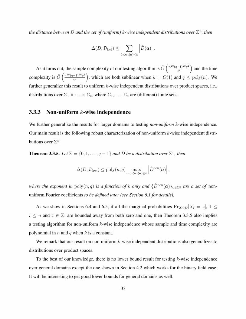
3.3.3 Non-uniform k-wise independence
We further generalize the results for larger domains to testing non-uniform k-wise independence.
Our main result is the following robust characterization of non-uniform k-wise independent distri-
butions over Σn.
Theorem 3.3.5. Let Σ = 0, 1, . . . , q − 1 and D be a distribution over Σn, then
∆(D,Dkwi) ≤ poly(n, q) maxa:0<wt(a)≤k
∣∣∣Dnon(a)∣∣∣ ,
where the exponent in poly(n, q) is a function of k only and Dnon(a)a∈Σn are a set of non-
uniform Fourier coefficients to be defined later (see Section 6.1 for details).
As we show in Sections 6.4 and 6.5, if all the marginal probabilities PrX∼D[Xi = z], 1 ≤
i ≤ n and z ∈ Σ, are bounded away from both zero and one, then Theorem 3.3.5 also implies
a testing algorithm for non-uniform k-wise independence whose sample and time complexity are
polynomial in n and q when k is a constant.
We remark that our result on non-uniform k-wise independent distributions also generalizes to
distributions over product spaces.
To the best of our knowledge, there is no lower bound result for testing k-wise independence
over general domains except the one shown in Section 4.2 which works for the binary field case.
It will be interesting to get good lower bounds for general domains as well.
33

3.3.4 Almost k-wise independence
A related problem, namely testing almost k-wise independence (see Section 7.1 for relevant defi-
nitions), admits a simple testing algorithm and a straightforward analysis. We include these results
in Chapter 7 for completeness.
3.4 Techniques
In this section we discuss the technical contributions of our work. For most parts of the thesis, we
are dealing with the following question: Given a distribution D which is close to k-wise indepen-
dence, how to find a sequence of operations which transform D into k-wise independent and incur
as small statistical difference as possible?
3.4.1 Previous techniques
Given a distribution D over the binary field which is not k-wise independent, a k-wise independent
distribution was constructed in [5] by mixing2 D with a series of carefully chosen distributions in
order to zero-out all the Fourier coefficients over subsets of size at most k. The total weight of the
distributions used for mixing is an upper bound on the distance of D from k-wise independence.
The distributions used for mixing are indexed by subsets S ⊂ 1, 2, . . . , n of size at most k. For
a given such subset S, the added distribution US is picked such that, on the one hand it corrects
the Fourier coefficient over S; on the other hand, US’s Fourier coefficient over any other subset is
zero. Using the orthogonality property of Hadamard matrices, one chooses US to be the uniform
distribution over all strings whose parity over S is 1 (or −1, depending on the sign of the distri-
bution’s bias over S). Although one can generalize it to work for prime fields, this construction
breaks down when the alphabet size is a composite number.
2Here “mixing” means replacing the distribution D with a convex combination of D and some other distribution.
34

3.4.2 Techniques for the binary domain case
Our upper and lower bounds on ∆(D,Dkwi), together with the proof techniques, may be of in-
dependent interest when interpreted as Fourier-analytic inequalities for bounded functions on the
hypercube. The harmonic analysis of such functions has been considered in the Computer Science
literature, e.g., in [27]. The connection to Fourier analysis comes from the basic fact that the biases
of a distribution D are equal to D’s Fourier coefficients (up to a normalization factor).
Bounds on ∆(D,Dkwi) may be viewed as part of the following general question: fix a family
F of functions on the hypercube and a subfamily H ⊂ F of functions defined via a restriction on
their Fourier coefficients. Then, for function f ∈ F , what is the `1 distance from f to its projection
in H , i.e., `1(f, H)?3 In our case F is the set of all functions mapping to [0, 1] and sum up to 1
(i.e., distributions), and H (i.e., k-wise independent distributions) further requires that the functions
have all Fourier coefficients over non-empty subsets of size at most k to be zero. Then, for example,
Parseval’s equality gives the following bound on the `2-norm: `2(f, H) ≥ ‖f≤k‖2 where f≤k(x) ,∑0<|S|≤k fSχS(x) is the truncation of f to the low-level Fourier spectrum. If the functions were
not restricted to mapping to [0, 1], then the lower bound is attainable thus making the inequality
an equality. However, the constraint that the functions under consideration are distributions makes
the problem much harder. Unfortunately, such a bound implies only very weak bounds for the
`1-norm.
In contrast, our upper bound on ∆(D,Dkwi) says that `1(f, H) ≤ ‖f≤k‖2 · O(logk/2 n). To
prove such an inequality, we proceed as follows. Given a distribution D = f , we approximate
D using a function D1, obtained by forcing all of D’s first k-level Fourier coefficients to zero
while keeping all others unchanged. Although D1 is not necessarily a probability distribution (it
may map some inputs to negative values), we show how to turn it back into a k-wise independent
distribution by “mending” it with a series of carefully chosen, small weight, k-wise independent
distributions in order to make all the values of D non-negative. By a deep result in Fourier analysis,
the Bonami-Beckner inequality, we bound the distance incurred by the “mending” process. Thus,
we are able to bound the total `1 distance of D to k-wise independence by the distance from D to
3The distance of a function to a set, `p(f,H), is defined to be minh∈H ‖f − h‖p.
35
D1 plus the “mending” cost.
Furthermore, our lower bound technique (employed by the Random Distribution Lemma) im-
plies that `1(f, H) ≥ ‖f≤k‖2‖f≤k‖∞
, which is already useful when we take f to be a uniform function on
a randomly chosen support. This inequality follows by taking the convolution of D = f with an
auxiliary function and then applying Young’s convolution inequality to lower bound the `1-norm
of D −D′, where D′ is the k-wise independent distribution closest to D.
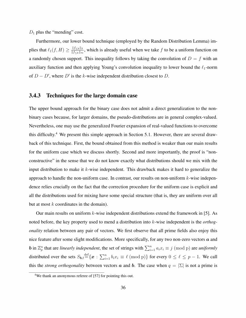
3.4.3 Techniques for the large domain case
The upper bound approach for the binary case does not admit a direct generalization to the non-
binary cases because, for larger domains, the pseudo-distributions are in general complex-valued.
Nevertheless, one may use the generalized Fourier expansion of real-valued functions to overcome
this difficulty.4 We present this simple approach in Section 5.1. However, there are several draw-
back of this technique. First, the bound obtained from this method is weaker than our main results
for the uniform case which we discuss shortly. Second and more importantly, the proof is “non-
constructive” in the sense that we do not know exactly what distributions should we mix with the
input distribution to make it k-wise independent. This drawback makes it hard to generalize the
approach to handle the non-uniform case. In contrast, our results on non-uniform k-wise indepen-
dence relies crucially on the fact that the correction procedure for the uniform case is explicit and
all the distributions used for mixing have some special structure (that is, they are uniform over all
but at most k coordinates in the domain).
Our main results on uniform k-wise independent distributions extend the framework in [5]. As
noted before, the key property used to mend a distribution into k-wise independent is the orthog-
onality relation between any pair of vectors. We first observe that all prime fields also enjoy this
nice feature after some slight modifications. More specifically, for any two non-zero vectors a and
b in Znp that are linearly independent, the set of strings with
∑ni=1 aixi ≡ j (mod p) are uniformly
distributed over the sets Sb,`def=x :
∑ni=1 bixi ≡ ` (mod p) for every 0 ≤ ` ≤ p − 1. We call
this the strong orthogonality between vectors a and b. The case when q = |Σ| is not a prime is
4We thank an anonymous referee of [57] for pointing this out.
36

less straightforward. The main difficulty is that the strong orthogonality between pairs of vectors
no longer holds, even when they are linearly independent5.
Suppose we wish to use some distribution Ua to correct the bias over a. A simple but important
observation is that we only need that Ua’s Fourier coefficient at b to be zero, which is a much
weaker requirement than the property of being strongly orthogonal between a and b. Using a
classical result in linear systems of congruences due to Smith [60], we are able to show that when
a satisfies gcd(a1, . . . , an) = 1 and b is not a multiple of a, the set of strings with∑n
i=1 aixi ≡
j (mod q) are uniformly distributed over Sb,` for `’s that lie in a subgroup of Zq (compared with
the uniform distribution over the whole group Zp for the prime field case). We refer to this as the
weak orthogonality between vectors a and b. To zero-out the Fourier coefficient at a, we instead
bundle the Fourier coefficient at a with the Fourier coefficients at `a for every ` = 2, . . . , q − 1,
and think of them as the Fourier coefficients of some function over the one-dimensional space Zq.
This allows us to upper bound the total weight required to simultaneously correct all the Fourier
coefficients at a and its multiples using only Ua. We also generalize the result to product spaces
Ω = Σ1 × · · · × Σn, which in general have different alphabets at different coordinates.
3.4.4 Techniques for non-uniform distributions
One possible way of extending the upper bounds of the uniform case to the non-uniform case would
be to map non-uniform probabilities to uniform probabilities over a larger domain. For example,
consider when q = 2 a distribution D with PrD[xi = 0] = 0.501 and PrD[xi = 1] = 0.499. We
could map xi = 0 and xi = 1 uniformly to 1, . . . , 501 and 502, . . . , 1000, respectively and test
if the transformed distribution D′ over 1, . . . , 1000 is k-wise independent. Unfortunately, this
approach produces a huge overhead on the distance upper bound, due to the fact that the alphabet
size (and hence the distance bound) blowup depends on the closeness of marginal probabilities
over different letters in the alphabet. However, in the previous example we should expect that D
behaves very much like the uniform case rather than with an additional factor of 1000 blowup in
the alphabet size.
5We say two non-zero vectors a and b in Znq are linearly dependent if there exist two non-zero integers s and t in
Zq such that sai ≡ tbi (mod q) for every 1 ≤ i ≤ n, and linearly independent if they are not linearly dependent
37

Instead we take the following approach. Consider a compressing/stretching factor for each
marginal probability PrD[xi = z], where z ∈ Σ and 1 ≤ i ≤ n. Specifically, let θi(z)def= 1
q PrD[xi=z]
so that θi(z) PrD[xi = z] = 1q, the probability that xi = z in the uniform distribution. If we mul-
tiply D(x) for each x in the domain by a product of n such factors, one for each coordinate, the
non-uniform k-wise independent distribution will be transformed into a uniform one. The hope is
that distributions close to non-uniform k-wise independent will also be transformed into distribu-
tions that are close to uniform k-wise independent. However, this could give rise to exponentially
large distribution weight at some points in the domain, making the task of estimating the relevant
Fourier coefficients intractable. Intuitively, for testing k-wise independence purposes, all we need
to know are the “local” weight distributions. To be more specific, for a vector a ∈ Σn, the support
set or simply support of a is supp(a)def=i ∈ [n] : ai 6= 0. For every non-zero vector a of weight
at most k, we define a new non-uniform Fourier coefficient at a in the following steps:
1. Project D to supp(a) to get Dsupp(a);
2. For every point in the support of Dsupp(a), multiply the marginal probability by the product
of a sequence of compressing/stretching factors, one for each coordinate in supp(a). Denote
this transformed distribution by D′supp(a);
3. Define the non-uniform Fourier coefficient of D at a to be the (uniform) Fourier coefficient
of D′supp(a) at a.
We then show a new characterization that D is non-uniform k-wise independent if and only
if all the first k levels non-zero non-uniform Fourier coefficients of D are zero. This enables us
to apply the Fourier coefficient correcting approach developed for the uniform case to the non-
uniform case. Loosely speaking, for any vector a, we can find a (small-weight) distribution Wa
such that mixing D′supp(a) with Wa zeroes-out the (uniform) Fourier coefficient at a, which is, by
definition, the non-uniform Fourier coefficient of D at a. But this Wa is the distribution to mix
with the “transformed” distribution, i.e., D′supp(a). To determine the distribution works for D, we
apply an inverse compressing/stretching transformation to Wa to get Wa. It turns out that mixing
Wa with the original distribution D not only corrects D’s non-uniform Fourier coefficient at a
38

but also does not increase D’s non-uniform Fourier coefficients at any other vectors except those
vectors whose supports are strictly contained in supp(a). Moreover, transforming from Wa to Wa
incurs at most a constant (independent of n) blowup in the total weight. Therefore we can start
from vectors of weight k and correct the non-uniform Fourier coefficients from level k to lower
levels. This process terminates after we finish correcting all vectors of weight 1 and thus obtain a k-
wise independent distribution. Bounding the total weight added during this process gives an upper
bound on the distance between D and non-uniform k-wise independence. We hope that the notion
of non-uniform Fourier coefficients may find other applications when non-uniform independence
is involved.
3.5 Query and time complexity analysis of the generic testing
algorithm
We now provide a detailed analysis of the query and time complexity analysis of the generic testing
algorithm as shown in Fig. 3-1. The main technical tool is the following standard Chernoff bound.
Theorem 3.5.1 (Chernoff Bound). Let X1, . . . , Xm be i.i.d. 0-1 random variables with E [Xi] = µ.
Let µ = 1m
∑mi=1 Xi. Then for all γ, 0 < γ < 1, we have Pr[|µ− µ| ≥ γµ] ≤ 2 · e− γ2µm
3 .
Theorem 3.5.2. Let D be a distribution over Σn where |Σ| = q and A be a subset of vectors in
Σn. Suppose the distance between D and the set of k-wise independent distributions satisfies the
following conditions:
• (completeness) For any 0 ≤ δ ≤ 1, if ∆(D,Dkwi) ≤ δ, then |D(a)| ≤ κδ for every a in A;
• (soundness) ∆(D,Dkwi) ≤ K maxa∈A
∣∣∣D(a)∣∣∣ , where K is a function of n, k, q and A.
Then for any 0 < ε ≤ 1, the generic testing algorithm draws6 m = O( q2K2
ε2log(q|A|)) inde-
pendent samples from D and runs in time O( q2K2|A|ε2
log(q|A|)) and satisfies the followings: If
6For all the cases studied in this thesis, the size of A is much larger than q, therefore we omit the factor q in thelogarithm in all the subsequent formulas.
39

∆(D,Dkwi) ≤ ε3κK
, then with probability at least 2/3, it outputs “Accept”; if ∆(D,Dkwi) > ε,
then with probability at least 2/3, it outputs “Reject”.
Proof. The algorithm is to sample D independently m times and use these samples to estimate,
for each a ∈ A, the Fourier coefficient of D at a. Then if maxa∈A
∣∣∣D(a)∣∣∣ ≤ 2ε
3K, the algorithm
accepts D; otherwise it rejects D. The running time bound follows from the fact that we need to
estimate |A| Fourier coefficients using m samples.
For every a ∈ A and 0 ≤ j ≤ q − 1, define a 0-1 indicator variable Ia,j(x), where x ∈ Σn,
which is 1 if a · x ≡ j (mod q) and 0 otherwise. Clearly Ia,jdef=E [Ia,j] = Pa,j . Let Pa,j =
1m
∑x∈Q Ia,j(x); that is, Pa,j is the empirical estimate of Pa,j . Since Pa,j ≤ 1, by Chernoff bound,
Pr[|Pa,j − Pa,j| > ε3qK
] < 23q|A| . By union bound, with probability at least 2/3, for every vector a
in A and every 0 ≤ j < q, |Pa,j − Pa,j| ≤ ε3qK
.
The following fact provides an upper bound of the error in estimating the Fourier coefficient at
a in terms of the errors from estimating Pa,j .
Fact 3.5.3. Let f, g : 0, . . . , q − 1 → R with |f(j) − g(j)| ≤ ε for every 0 ≤ j ≤ q − 1. Then∣∣∣f(`)− g(`)∣∣∣ ≤ qε for all 0 ≤ ` ≤ q − 1.
Proof. Let h = f − g, then |h(j)| ≤ ε for every j. Therefore,
|f(`)− g(`)|
= |h(`)| = |q−1∑j=0
h(j)e2πiq
`j|
≤q−1∑j=0
|h(j)e2πiq
`j| =q−1∑j=0
|h(j)|
≤q−1∑j=0
ε = qε.
Let ¯D(a) be the estimated Fourier coefficient computed from Pa,j . Fact 3.5.3 and (2.3) then
imply that with probability at least 2/3,∣∣∣ ¯D(a)− D(a)
∣∣∣ ≤ ε3K
for every a in A.
40

Now if ∆(D,Dkwi) ≤ ε3κK
, then by our completeness assumption, we have maxa∈A
∣∣∣D(a)∣∣∣ ≤
ε3K
. Taking the error from estimation into account, maxa∈A
∣∣∣ ¯D(a)∣∣∣ ≤ 2ε
3Kholds with probability
at least 2/3. Therefore with probability at least 2/3, the algorithm returns “Accept”.
If ∆(D,Dkwi) > ε, then by our soundness assumption, maxa∈A
∣∣∣D(a)∣∣∣ > ε
K. Again with
probability at least 2/3, maxa∈A
∣∣∣ ¯D(a)∣∣∣ > 2ε
3Kfor every a in A, so the algorithm returns “Reject”.
41

42

Chapter 4
Binary Domains
In this chapter, we study the problem of testing whether a distribution over a Boolean cube is
k-wise independent or δ-far from from k-wise independence. Our upper bound and lower bound
results for testing are based on new upper and lower bounds on ∆(D,Dkwi) in term of D’s first
k-level biases (or equivalently, Fourier coefficients. See below for definition of biases). We present
our upper bounds in Section 4.1 and lower bounds in Section 4.2.
4.1 Upper bounds on testing k-wise independence
4.1.1 Characterizing k-wise independence by biases
We use the notion of a bias over a set T which is a measure of the parity imbalance of the distribu-
tion over the set T of variables:
Definition 4.1.1. For a distribution D over 0, 1n, the bias of D over a non-empty set T ⊆ [n] is
defined as biasD(T ) , Prx←D[⊕i∈T xi = 0] − Prx←D[⊕i∈T xi = 1]. We say biasD(T ) is an l-th
level bias if |T | = l.
Up to a normalization factor, the biases are equal to the Fourier coefficients of the distribution
function D. More precisely, D(T ) = 12n biasD(T ), for T 6= ∅. Thus, we sometimes use the terms
biases and Fourier coefficients interchangeably. The following well-known facts relate biases to
43

k-wise independence:
Fact 4.1.2. A distribution is k-wise independent iff all the biases over sets T ⊂ [n], 0 < |T | ≤ k,
are zero. In particular, for the uniform distribution Un, biasUn(T ) = 0 for all T .
By the alternative definition of statistical distance, we immediately have the following.
Fact 4.1.3. The distance between D and k-wise independence can be lower bounded by
∆(D,Dkwi) ≥1
2max
T⊆[n],0<|T |≤kbiasD(T ).
4.1.2 Upper bound the distance to k-wise independence
In this section, we first prove an upper bound on ∆(D,Dkwi), then present our testing algorithm as
well as the sample and time complexity of our algorithm. For brevity, let b1 ,∑|S|≤k |biasD(S)|
and b2 ,√∑
|S|≤k biasD(S)2. Note that b2 ≤ b1 ≤√
Mn,kb2 < nk/2b2.
The only previously known upper bound for ∆(D,Dkwi) is given in [5], where it is implicitly
shown that ∆(D,Dkwi) ≤ b1. Our new bound is the following.
Theorem 4.1.4 (Upper Bound on Distance). The distance between a distribution D and k-wise
independence can be upper bounded by
∆(D,Dkwi) ≤ O
(log n)k/2
√∑|S|≤k
biasD(S)2
.
Consequently,
∆(D,Dkwi) ≤ O((n log n)k/2
)max|S|≤k
|biasD(S)|.
Since b2 is always smaller than or equal to b1, our upper bound is no weaker than that of [5] up
to a polylogarithmic factor. However, for many distributions of interest, b2 is much smaller than
b1 (e.g., when all the biases are roughly of the same magnitude, as in the case of random uniform
distributions, then b2 = O∗(b1/nk/2)).
The basic ideas of our proof are the following. We first operate in the Fourier space to construct
a “pseudo-distribution” D1 by forcing all the first k-level Fourier coefficients to be zero. D1 is not
44

a distribution because it may assume negative values at some points. We then correct all these neg-
ative points by a series of convex combinations of D1 with k-wise independent distributions. This
insures that all the first k-level Fourier coefficients remain zero, while increasing the weights at
negative points so that they assume non-negative values. During the correction, we distinguish be-
tween two kinds of points which have negative weights: Light points whose magnitudes are small
and heavy points whose magnitudes are large. We use two different types of k-wise independent
distributions to handle these two kinds of points. Using Bonami-Beckner’s inequality, we show
that only a small number of points are heavy, thus obtaining a better bound for ∆(D,Dkwi).
Proof of Theorem 4.1.4. The following lemma bounds the `1-distance between a function and its
convex combination with other distributions.
Lemma 4.1.5. Let f be a real function defined over domain D = 0, 1n such that∑
x∈D f(x) =
1. Let D1, . . . , D` be distributions over the same domain D. Suppose there exist positive real
numbers w1, . . . , w` such that D′ , 1
1+P`
i=1 wi(f +
∑`i=1 wiDi) is non-negative for all x ∈ D.
Then 2n
2‖f(x)−D′(x)‖1 ≤
∑`i=1 wi.
Proof. ‖f(x)−D′(x)‖1 = ‖∑`
i=i wi(D′ −Di)‖1 ≤
∑`i=i wi‖D′ −Di‖1 ≤ 2−n+1
∑`i=i wi.
We first construct a real function D1 : 0, 1n → R based on D but forcing all its first k-level
biases to be zero. D1 is defined by explicitly specifying all of its Fourier coefficients:
D1(S) =
0, if S 6= ∅ and |S| ≤ k
D(S), otherwise.
Since D1(∅) = D(∅) = 12n , we have
∑x D1(x) = 1. Note that in general D1 is not a distri-
bution because it is possible that for some x, D1(x) < 0. By Parseval’s equality, ‖D − D1‖2 =
12n
√∑|T |≤k biasD(T )2 = 1
2n b2. Hence by the Cauchy-Schwarz inequality, we can upper bound the
`1-norm of D −D1 as ‖D −D1‖1 ≤ 2−n · b2. Now we define another function D2 : 0, 1n → R
45

as
D2(S) =
D(S), if S 6= ∅ and |S| ≤ k
0, otherwise.
By the linearity of the Fourier transform, D1(x) + D2(x) = D(x). Since D(x) ≥ 0 for all
x ∈ 0, 1n, we have D1(x) ≥ −D2(x). By the Fourier transform,
|D2(x)| =
∣∣∣∣∣∣ 1
2n
∑1≤|S|≤k
biasD(S)χS(x)
∣∣∣∣∣∣≤ 1
2n
∑1≤|S|≤k
|biasD(S)| = 1
2nb1.
Hence the magnitudes of D1(x)’s negative points are upper bounded by 12n b1, i.e. D2(x) ≥ − 1
2n b1.
By the linearity of the Fourier transform, if we define a function D′ as the convex combination
of D1 with some k-wise independent distributions so that D′ is non-negative, then D′ will be a
k-wise independent distribution, since all the Fourier coefficients of D′ on the first k levels are
zero.
If we use a uniform distribution to correct all the negative weights of D1, then we will get
an upper bound almost the same (up to a factor of 3/2) as that of [5]. To improve on this, we
distinguish between two kinds of points where D1 may assume negative weights: heavy points
and light points. Let λ = (2√
log n)k. We call a point x heavy if D1(x) ≤ −λb2/2n, and light
if −λb2/2n < D1(x) < 0. For light points, we still use a uniform distribution to correct them;
but for each heavy point, say z, we will use a special k-wise independent distribution UBCH-z(x),
constructed in [3]:
Theorem 4.1.6 ([3]). For any z ∈ 0, 1n, there is a k-wise independent distribution UBCH-z(x)
over 0, 1n such that UBCH-z(z) = 1| Supp(UBCH-z)| = Ω(n−bk/2c). 1
1Note that, as shown in [21, 3], the support sizes of such constructions are essentially optimal.
46

Thus, we define D′ by
D′(x) =D1(x) + λb2Un(x) +
∑z is heavy wzUBCH-z(x)
1 + λb2 +∑
z is heavy wz
.
We set wz = | Supp(UBCH-z)|2n b1. Since D1(x) ≥ − b1
2n , one can check that D′(x) is non-negative
for both heavy and light points. Hence D′ is a k-wise independent distribution.
Next we bound the number of heavy points. Note that this number is at most the number of
points at which D2(x) ≥ λb2/2n. Observe that D2(x) has only the first k-level Fourier coefficients,
hence we can use Bonami-Beckner’s inequality to bound the probability of |D2(x)| assuming large
values, and thus the total number of heavy points.
First we scale D2(x) to make it of unit `2-norm. Define f(x) = 2n
b2D2(x). Then
‖f‖2 =2n
b2
‖D2‖2 =2n
b2
√1
2n
∑x∈0,1n
D2(x)2
=2n
b2
√1
22n
∑1≤|S|≤k
biasD(S)2 = 1,
where the second to last step follows from Parseval’s equality. Now using the higher moment
inequality method, we have, for even p,
Pr[|f(x)| ≥ λ] ≤ Ex [|f(x)|p]λp
=‖f‖p
p
λp.
By Theorem 2.2.6, ‖f‖p ≤(√
p− 1)k ‖f‖2 =
(√p− 1
)k. Plug in λ = (2√
log n)k and p = log n,
and without loss of generality, assume that p is even, then we have
Pr[|f(x)| ≥ 2k logk/2 n] ≤ (p− 1)pk/2
λp<
ppk/2(2√
log n)pk
= (1
2)k log n =
1
nk.
47
Therefore,
Pr
[D1(x) ≤ −2k(log n)k/2 b2
2n
]≤ Pr
[D2(x) ≥ 2k(log n)k/2b2/2
n]
≤ Pr[|D2(x)| ≥ 2k(log n)k/2b2/2
n]
= Pr[|f(x)| ≥ 2k(log n)k/2
]< 1/nk.
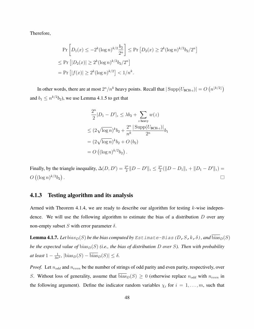
In other words, there are at most 2n/nk heavy points. Recall that | Supp(UBCH-z)| = O(nbk/2c)
and b1 ≤ nk/2b2), we use Lemma 4.1.5 to get that
2n
2|D1 −D′|1 ≤ λb2 +
∑z heavy
w(z)
≤ (2√
log n)kb2 +2n
nk
| Supp(UBCH-z)|2n
b1
= (2√
log n)kb2 + O (b2)
= O((log n)k/2b2
).
Finally, by the triangle inequality, ∆(D, D′) = 2n
2‖D −D′‖1 ≤ 2n
2(‖D −D1‖1 + ‖D1 −D′‖1) =
O((log n)k/2b2
).
4.1.3 Testing algorithm and its analysis
Armed with Theorem 4.1.4, we are ready to describe our algorithm for testing k-wise indepen-
dence. We will use the following algorithm to estimate the bias of a distribution D over any
non-empty subset S with error parameter δ.
Lemma 4.1.7. Let biasD(S) be the bias computed by Estimate-Bias(D,S,k,δ), and biasD(S)
be the expected value of biasD(S) (i.e., the bias of distribution D over S). Then with probability
at least 1− 13nk , |biasD(S)− biasD(S)| ≤ δ.
Proof. Let nodd and neven be the number of strings of odd parity and even parity, respectively, over
S. Without loss of generality, assume that biasD(S) ≥ 0 (otherwise replace nodd with neven in
the following argument). Define the indicator random variables χi for i = 1, . . . ,m, such that
48

Algorithm Estimate-Bias(D,S,k,δ)
1. Set m = O((k log n)/δ2
).
2. Set nodd = 0.(Assume the sample set is Q = X1, . . . , Xm)
3. For i = 1 to m
• If ⊕j∈SXij = 1, nodd = nodd + 1.
4. Output biasD(S) = 2noddm − 1.
Figure 4-1: Algorithm for estimating the bias over an index subset S.
Algorithm Test-KWI-Closeness(D,k,δ)
1. From D, draw a set Q of samples of size |Q| = O(k log n/δ′2
), where δ′ = δ
3Ck(n log n)k/2 .
2. For each non-empty subset S ⊆ [n], |S| ≤ k, use Q to estimate biasD(S) to within anadditive term of δ′.
3. If maxS |biasD(S)| ≤ 2δ′ return “Yes”; else return “No”.
Figure 4-2: Algorithm for testing if a distribution is k-wise independent.
χi = ⊕j∈SX ij . It is clear that χi are 0/1 random variables and E [χi] = nodd/m ≥ 1/2. Now
applying Chernoff bound to χi gives the desired result, since biasD(S) = 2E [χi]− 1.
Now we are ready to describe the algorithm of testing closeness to k-wise independence, which
(implicitly) uses Estimate-Bias as a subroutine.
The algorithm is simple in nature: it estimates all the first k-level biases of the distribution and
returns “Yes” if they are all small. Let Ck be the hidden constant in O (·) in the second part of
Theorem 4.1.4.
Next we prove the correctness of Test-KWI-Closeness(D,k,δ).
Theorem 4.1.8. Let D be a distribution over 0, 1n. If ∆(D,Dkwi) ≤ 2δ3Ck(n log n)k/2 , then Test-KWI-Closeness
accepts with probability at least 2/3; If ∆(D,Dkwi) > δ, then Test-KWI-Closeness accepts
with probability at most 1/3. Furthermore, the sample complexity of Test-KWI-Closeness is
O(kCk(log n)k+1nk/δ2) = O∗(nk
δ2 ), and running time of Test-KWI-Closeness is O∗(n2k
δ2 ).
49

Proof of Theorem 4.1.8. The running time and sample complexity analysis is straightforward. If
∆(D,Dkwi) ≤ 2δ3Ck(n log n)k/2 , then by Fact 4.1.3, biasD(S) ≤ δ
3Ck(n log n)k/2 for every 1 ≤ |S| ≤ k.
By Lemma 4.1.7, |biasD(S) − biasD(S)| ≤ δ3Ck(n log n)k/2 with probability at least 1 − 1
3nk . Thus
union bound gives, with probability at least 1 −Mn,k1
3nk ≥ 2/3 (since Mn,k ≤ nk), |biasD(S) −
biasD(S)| ≤ δ3Ck(n log n)k/2 holds for each S. This implies that, for every non-empty S of size at
most k, Ck(n log n)k/2|biasD(S)| ≤ 23δ. Therefore, the algorithm accepts.
If ∆(D,Dkwi) > δ, by Theorem 4.1.4, Ck(n log n)k/2 maxS 6=∅,|S|≤k |biasD(S)| > δ. A similar
analysis shows that with probability at least 2/3, Ck(n log n)k/2 maxS 6=∅,|S|≤k |biasD(S)| > 23δ and
hence the algorithm rejects.
Note that for constant k, Test-KWI-Closeness gives an algorithm testing k-wise indepen-
dence running in time sublinear (in fact, polylogarithmic) in the size of the support (N = 2n) of
the distribution.
4.2 Lower bounds on testing k-wise independence
In this section, we prove a lower bound on the sample complexity of our testing algorithm. How-
ever, we first motivate our study from the perspective of real functions defined over the boolean
cube.
The upper bound given in Theorem 4.1.4 naturally raises the following question: Can we
give a lower bound on ∆(D,Dkwi) in term of the first k-level biases of D? The only known
answer to this question we are aware of is the folklore lower bound in Fact 4.1.3: ∆(D,Dkwi) ≥12max1≤|S|≤k |biasD(S)|. This bound is too weak for many distributions, as demonstrated in [5],
who gave a family of distributions that have all the first k-level biases at most O(
1n1/5
), but are at
least 1/2-away from any k-wise independent distribution. Their proof is based on a min-entropy
argument, which seems to work only for distributions with small support size.
In fact, this statistical distance lower bound problem can be put into a more general framework.
Given a function f : 0, 1n → R, can we give a lower bound on ‖f‖1 if only the first k-level
Fourier coefficients of f are known? Hausdorff-Young’s inequality gives ‖f‖1 ≥ ‖f‖∞, which
50

is equivalent to the bound stated in Fact 4.1.3. We develop a new approach to lower bound ‖f‖1
in terms of f ’s first k-level Fourier coefficients. Our method works for general k and is based on
convolving f with an auxiliary function and then applying Young’s convolution inequality. Our
main result of this section is the following lower bound on distances between random uniform
distributions and k-wise independence, which is the basis of our sample lower bound result, Theo-
rem 4.2.15. Note that by Theorem 4.1.4, this bound is almost tight as implied by our upper bound
result.
Lemma 4.2.1 (Random Distribution Lemma). Let k > 2. Let Q =Mn,k
nδ2 with δ = o(1/n). If we
sample uniformly at random Q strings from 0, 1n to form a random multi-setQ and let UQ(x) be
the uniform distribution overQ, then for all large enough n, PrQ[∆(UQ,Dkwi) > 0.09δ] = 1−o(1).
4.2.1 New lower bounds for ∆(D,Dkwi)
In this section, we will develop a new framework to prove lower bound on the distance between a
distribution and k-wise independent distributions and apply this method to prove Theorem 4.2.4.
In fact, our techniques developed here may be of independent interest: We give a new lower bound
on the `1-norm of a function f : 0, 1n → R in terms of f ’s first k-level Fourier coefficients. Our
method is based on convolving f with an auxiliary function and applying Young’s convolution
inequality:
Theorem 4.2.2 (Young’s convolution inequality). Let 1 ≤ p, q, r ≤ ∞, such that 1r
= 1p
+ 1q− 1.
Then for any f, g : 0, 1n → R, ‖f ∗ g‖r ≤ ‖f‖p‖g‖q.
Given a distribution D over 0, 1n. Let D′ be the k-wise independent distribution which is
closest to D, i.e., ∆(D,Dkwi) = ∆(D, D′) = 12‖D −D′‖1. Define f(x) = D(x) −D′(x). Then
we have
f(S) =1
2nbiasD(S), for all non-empty subsets S with |S| ≤ k,
and
∆(D,Dkwi) =1
2
∑x∈0,1n
|f(x)| = 2n−1‖f‖1.
51
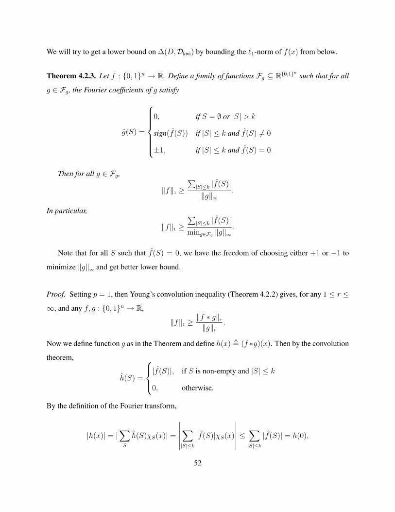
We will try to get a lower bound on ∆(D,Dkwi) by bounding the `1-norm of f(x) from below.
Theorem 4.2.3. Let f : 0, 1n → R. Define a family of functions Fg ⊆ R0,1n such that for all
g ∈ Fg, the Fourier coefficients of g satisfy
g(S) =
0, if S = ∅ or |S| > k
sign(f(S)) if |S| ≤ k and f(S) 6= 0
±1, if |S| ≤ k and f(S) = 0.
Then for all g ∈ Fg,
‖f‖1 ≥∑|S|≤k |f(S)|‖g‖∞
.
In particular,
‖f‖1 ≥∑|S|≤k |f(S)|
ming∈Fg ‖g‖∞.
Note that for all S such that f(S) = 0, we have the freedom of choosing either +1 or −1 to
minimize ‖g‖∞ and get better lower bound.
Proof. Setting p = 1, then Young’s convolution inequality (Theorem 4.2.2) gives, for any 1 ≤ r ≤
∞, and any f, g : 0, 1n → R,
‖f‖1 ≥‖f ∗ g‖r
‖g‖r
.
Now we define function g as in the Theorem and define h(x) , (f ∗g)(x). Then by the convolution
theorem,
h(S) =
|f(S)|, if S is non-empty and |S| ≤ k
0, otherwise.
By the definition of the Fourier transform,
|h(x)| = |∑
S
h(S)χS(x)| =
∣∣∣∣∣∣∑|S|≤k
|f(S)|χS(x)
∣∣∣∣∣∣ ≤∑|S|≤k
|f(S)| = h(0),
52

since for all S ⊆ [n], χS(0) = 1 and the evaluation of any function at 0 is simply the sum of all its
Fourier coefficients. Thus, ‖h‖∞ = h(0) =∑|S|≤k |f(S)|. Now take r tending to infinity, we get
‖f‖1 ≥∑|S|≤k |f(S)|‖g‖∞
.
Thus we get a lower bound for ∆(D,Dkwi):
Theorem 4.2.4. Let D be a distribution over 0, 1n, and let Fg be defined as in Theorem 4.2.3
but replacing f(S) with biasD(S). Then for all g ∈ Fg, ∆(D,Dkwi) ≥12
P|S|≤k |biasD(S)|‖g‖∞ .
If all the low level Fourier coefficients of f are non-zero, then there is a unique g ∈ Fg that
corresponds to f . Otherwise, there may be many g’s in Fg all correspond to f . If this is the case,
for the purpose of proving lower bound, we may pick the one with the smallest infinity norm. On
the other hand, there are many different f ’s that correspond to the same g. A nice property of
function g is that only the first k-level Fourier coefficients are non-zero and all these coefficients
are in −1, 1. By the monotonicity of norms and Parseval’s equality, we have ‖g‖∞ ≥ ‖g‖2 =√∑1 ≤|S|≤k 1 =
√Mn,k. And a trivial upper bound is ‖g‖∞ ≤ Mn,k. Note that if ‖g‖∞ Mn,k,
then our new lower bound on ∆(D,Dkwi) probably will give a much better bound than the trivial
lower bound ∆(D,Dkwi) ≥ 12maxS |biasD(S)|. Next we will provide some evidence showing the
strength of our new lower bound: among 2Mn,k = 2O(nk) possible g’s, at most an exponentially
small portion of them may have ‖g‖∞ = Ω(√
nMn,k). Thus most g’s will give good lower bound.
Theorem 4.2.5. Let g be an Mn,k-dimensional vector with its Mn,k components being g(x)’s non-
zero Fourier coefficients, then for all c > 0 and for all sufficiently large n,
Prg∈R−1,1Mn,k
[‖g‖∞ > 1.18
√c + 1
√nMn,k
]< 2−cn.
Proof. We will need the following simple Chernoff-type tail bound (see Corollary A.1.2 of [6])
Lemma 4.2.6. Let xi, 1 ≤ i ≤ m, be mutually independent random variables with Pr[xi = 1] =
53
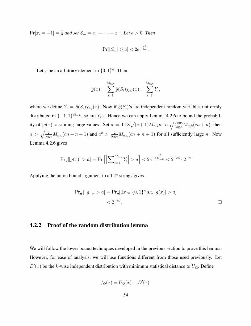
Pr[xi = −1] = 12
and set Sm = x1 + · · ·+ xm. Let a > 0. Then
Pr[|Sm| > a] < 2e−a2
2m .
Let x be an arbitrary element in 0, 1n. Then
g(x) =
Mn,k∑i=1
g(Si)χSi(x) =
Mn,k∑i=1
Yi,
where we define Yi = g(Si)χSi(x). Now if g(Si)’s are independent random variables uniformly
distributed in −1, 1Mn,k , so are Yi’s. Hence we can apply Lemma 4.2.6 to bound the probabil-
ity of |g(x)| assuming large values. Set a = 1.18√
(c + 1)Mn,kn >√
2.005log e
Mn,k(cn + n), then
a >√
2log e
Mn,k(cn + n + 1) and a2 > 2log e
Mn,k(cn + n + 1) for all sufficiently large n. Now
Lemma 4.2.6 gives
Prg[|g(x)| > a] = Pr[∣∣∣∑Mn,k
i=1Yi
∣∣∣ > a]
< 2e− a2
2Mn,k < 2−cn · 2−n
Applying the union bound argument to all 2n strings gives
Prg [‖g‖∞ > a] = Prg[∃x ∈ 0, 1n s.t. |g(x)| > a]
< 2−cn.
4.2.2 Proof of the random distribution lemma
We will follow the lower bound techniques developed in the previous section to prove this lemma.
However, for ease of analysis, we will use functions different from those used previously. Let
D′(x) be the k-wise independent distribution with minimum statistical distance to UQ. Define
fQ(x) = UQ(x)−D′(x).
54
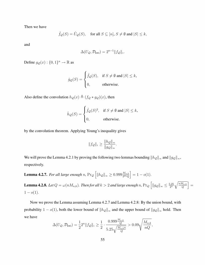
Then we have
fQ(S) = UQ(S), for all S ⊆ [n], S 6= ∅ and |S| ≤ k,
and
∆(UQ,Dkwi) = 2n−1‖fQ‖1.
Define gQ(x) : 0, 1n → R as
gQ(S) =
fQ(S), if S 6= ∅ and |S| ≤ k,
0, otherwise.
Also define the convolution hQ(x) , (fQ ∗ gQ)(x), then
hQ(S) =
fQ(S)2, if S 6= ∅ and |S| ≤ k,
0, otherwise.
by the convolution theorem. Applying Young’s inequality gives
‖fQ‖1 ≥‖hQ‖∞‖gQ‖∞
.
We will prove the Lemma 4.2.1 by proving the following two lemmas bounding ‖hQ‖∞ and ‖gQ‖∞,
respectively.
Lemma 4.2.7. For all large enough n, PrQ
[‖hQ‖∞ ≥ 0.999
Mn,k
22nQ
]= 1− o(1).
Lemma 4.2.8. Let Q = ω(nMn,k). Then for all k > 2 and large enough n, PrQ
[‖gQ‖∞ ≤ 5.25
2n
√nMn,k
Q
]=
1− o(1).
Now we prove the Lemma assuming Lemma 4.2.7 and Lemma 4.2.8: By the union bound, with
probability 1 − o(1), both the lower bound of ‖hQ‖∞ and the upper bound of ‖gQ‖∞ hold. Then
we have
∆(UQ,Dkwi) =1
22n‖fQ‖1 ≥
1
2·
0.999Mn,k
Q
5.25√
Mn,kn
Q
> 0.09
√Mn,k
nQ,
55

as desired.
In the following proofs of Lemma 4.2.7 and Lemma 4.2.8, we will assume that all the elements
in multiset Q are distinct. This will not affect our results, since by the Birthday paradox, the
probability of seeing a collision in Q is o(1).
Proof of Lemma 4.2.7 We prove the lower bound of ‖hQ‖∞ by computing the expectation and
variance of ‖hQ‖∞. Then a simple application of Chebyshev’s inequality gives the desired bound.
The calculations are straightforward but rather tedious.
Proof of Lemma 4.2.7. By the definition of Fourier transform
|hQ(x)| =
∣∣∣∣∣∣∑
1≤|S|≤k
hQ(S)χS(x)
∣∣∣∣∣∣ ≤∑
1≤|S|≤k
∣∣∣hQ(S)∣∣∣ =
∑1≤|S|≤k
hQ(S) = hQ(0).
Therefore
‖hQ‖∞ = hQ(0) =∑
1≤|S|≤k
fQ(S)2.
Then for all non-empty subset S with |S| ≤ k,
fQ(S) =1
2n
∑x∈0,1n
UQ(x)χS(x)
=1
2nQ
∑x∈Q
χS(x);
and
fQ(S)2 =1
22n
∑x,y∈0,1n
UQ(x)χS(x)UQ(y)χS(y)
=1
22nQ2
∑x,y∈Q
χS(x)χS(y);
To facilitate the calculation of the expectation and variance of ‖hQ‖∞, we first state two simple
technical claims.
56

Claim 4.2.9. Let x and y be two distinct strings chosen uniformly at random from 0, 1n, then for
all n > 1, x + y is equal to every element in 0, 1n \ 0n with equal probability.
Proof. First we fix an x, then the map y → x+y is a one-to-one correspondence between 0, 1n\
x and 0, 1n \ 0n. Then notice that y equals every element in 0, 1n \ x with equal
probability.
Claim 4.2.10. Let x, y, x′ and y′ be four distinct strings chosen uniformly at random from 0, 1n.
Then for all n > 2, x + y + x′ + y′ is equal to every element in 0, 1n with equal probability.
Proof. Let z1 = x+y. By claim 4.2.9, z1 equals all strings in 0, 1n\0nwith equal probability.
Then z1 + x′ equals all strings in 0, 1n \ x′ with equal probability. But x′ takes all values in
0, 1n equally often, so is z1 +x′ = x+ y +x′. Therefore x+ y +x′+ y′ is uniformly distributed
over 0, 1n.
Proposition 4.2.11. The expectation of ‖hQ‖∞ satisfies that
EQ [‖hQ‖∞] =Mn,k
22nQ(1− Q− 1
2n − 1).
Proof. We have
EQ [‖hQ‖∞] = EQ
∑1≤|S|≤k
fQ(S)2
=
1
22nQ2EQ
∑1≤|S|≤k
∑x,y∈Q
χS(x)χS(y)
=
Mn,k
22nQ+
1
22nQ2EQ
∑1≤|S|≤k
∑x,y∈Q,x 6=y
χS(x)χS(y)
=
Mn,k
22nQ+
1
22nQ2EQ
∑1≤|S|≤k
∑x∈Q
∑z 6=0n,z−x∈Q
χS(z)
=
Mn,k
22nQ+
Mn,kQ(Q− 1)
22nQ2Ez 6=0n [χS(z)] .
57

By Claim 4.2.9, z is uniformly distributed over 0, 1n\0n. Since for any S 6= ∅,∑
z∈0,1n χS(z) =
0, hence∑
z∈0,1n\0n χS(z) = −1, and Ez∈0,1n\0n [χS(z)] = − 12n−1
. Then we have
EQ [‖hQ‖∞] =Mn,k
22nQ(1− Q− 1
2n − 1).
This completes the proof.
Proposition 4.2.12. The expectation of ‖hQ‖2∞ satisfies that
EQ[‖hQ‖2
∞
]=
M2n,k
24nQ2(1− Q− 1
2n − 1)2 +
2Mn,kQ(Q− 1)
24nQ4(1− 2(Q− 2)
2n − 1)− Mn,k(Q− 1)2
24n(2n − 1)2Q2
=M2
n,k
24nQ2(1− Q− 1
2n − 1)2 +
2Mn,k
24nQ2(1− o(1)).
Proof.
EQ[‖hQ‖2
∞
]= EQ
(∑
1≤|S|≤k
fQ(S)2)2
= EQ
∑1≤|S|≤k
∑1≤|T |≤k
fQ(S)2fQ(T )2
=
1
24nQ4EQ
∑1≤|S|≤k
∑1≤|T |≤k
∑x,y∈Q
∑x′,y′∈Q
χS(x + y)χT (x′ + y′)
.
Then one can distinguish between 12 different cases and calculate their expectations respectively.
We omit the details here.
Therefore we have
Var(‖hQ‖∞) =1
24n
2Mn,k
Q2(1− o(1)),
and
σ(‖hQ‖∞) =1
22n
√2Mn,k
Q(1− o(1)).
Finally we apply Chebyshev’s inequality, which states that for any t > 0 Pr[|X − E [X] | >
58

tσ(X)] < 1t2
, to ‖hQ‖∞ to finish the proof of Lemma 4.2.7.
Proof of Lemma 4.2.8 A simple calculation shows that gQ(x) equals a summation of Q indepen-
dent random variables Y1, . . . , YQ determined by the random subsetQ, where−Mn,k ≤ Yi ≤ Mn,k.
However, a direct application of Hoeffding’s bound to the sum can only gives ‖gQ‖∞ = O (Mn,k),
thus ∆(UQ,Dkwi) = Ω( 1Q
), which is too weak. We improve on this is by noticing that the variance
of Yi is small, thus Bernstein’s inequality [13] gives a better bound.
Proof of Lemma 4.2.8. Fix an arbitrary x ∈ 0, 1n. Then
gQ(x) =∑
1≤|S|≤k
fQ(S)χS(x)
=1
2n
∑1≤|S|≤k
∑y∈0,1n
UQ(y)χS(x)χS(y)
=1
2nQ
∑1≤|S|≤k
∑y∈Q
χS(x + y)
=1
2nQ
∑y∈Q
∑1≤|S|≤k
χS(x + y)
=1
2nQ
∑y∈Q
Yx(y),
where Yx(y) ,∑
1≤|S|≤k χS(x+y). Note that the summation is over independent random variables
Yx(y) in Q.
If we apply the Hoeffding bound directly to the sum, we would not get the desired result.
Instead, we will employ the following Bernstein’s inequality [13], which gives a better bound on
the sum of independent random variables when we have a good bound on the variance of the
random variables being summed.
Theorem 4.2.13 (Bernstein’s inequality). Let X1, . . . , XQ be independent real-valued random
variables such that |Xi| ≤ C for all 1 ≤ i ≤ Q. Let σ2 = 1Q
∑Qi=1 Var(Xi). Then for any
t > 0
Pr[|Q∑
i=1
Xi − E [X] | > Qt] ≤ e− Qt2
2σ2+2Ct3
59

We next compute the expectation and variance of Yx(y).
Ey [Yx(y)] = Ey
∑1≤|S|≤k
χS(y)
=∑
1≤|S|≤k
Ey [χS(y)] =∑
1≤|S|≤k
0 = 0,
and
Ey
[Yx(y)2
]= Ey
∑1≤|S|≤k
χS(y)
2= Ey
∑1≤|S|,|T |≤k
χS(y)χT (y)
= Ey
∑1≤|S|≤k
χS(y)2
+ Ey
∑1≤|S|≤k
∑S′ 6=∅
χS′(y)
(S ′ , S∆T )
= Mn,k + 0
= Mn,k.
By setting t = 5.25√
Mn,kn
Qand noticing that Q = ω(nMn,k), we have
Pr
[∣∣∣∣∣∑y∈Q
Yx(y)
∣∣∣∣∣ ≥ 5.25Q
√Mn,kn
Q
]≤ 2−no(1).
It follows that, with probability 1− o(1), for all x
2n|gQ(x)| ≤ 5.25
√Mn,kn
Q.
i.e. with probability 1− o(1),
‖gQ‖∞ ≤5.25
2n
√Mn,kn
Q.
This completes the proof of Lemma 4.2.8.
60

Tightness of the Lemma 4.2.1 Our lower bound on the statistical distance between a random
distribution and k-wise independent distributions is almost tight due to the following proposition
Proposition 4.2.14. Let S be a random multiset formed by uniformly sampling Ω(k(log n)k+1nk/δ2)
times from 0, 1n. Then with high probability, US is δ-close to k-wise independent.
Proof. By Chernoff bound, for every S ⊆ [n], |S| ≤ k, S 6= ∅, with probability at least (1− 13nk ),
|biasUS(S)| ≤ O(δ/(n log n)k/2). By a union bound argument, this holds for all S with probability
at least 2/3. Applying Theorem 4.1.4 gives the desired result.
Sample lower bound
Now we apply Random Distribution Lemma to prove a lower bound on the sample complexity of
testing k-wise independence.
Theorem 4.2.15 (Sample Lower Bound). For k > 2 and δ = o(1/n), testing k-wise independence
requires at least |Q| = Ω(
1δ· (n
k)
k−12
)samples from the distribution.
Our lower bound result rules out the possibility of polynomial time testing algorithms for k =
ω(1).
Proof of Theorem 4.2.15. We will show that if the algorithm makes too few queries, then it can-
not successfully distinguish between two distributions far apart with high probability. Consider
the following two distributions. The first one is the uniform distribution Un over 0, 1n. Ob-
viously, Un is k-wise independent for all 1 ≤ k ≤ n. The second distribution UQ is a uni-
form distribution over a multiset Q, where Q is constructed by uniformly and randomly sampling
Z =(
0.09δ
(nk)
k−12
)2
≤ 0.092 Mn,k
nδ2 times from 0, 1n. By Lemma 4.2.1, with probability 1− o(1),
UQ is at least δ-far from any k-wise independent distribution. Now let A be any algorithm that
makes Q = o(√
Z) = o(
1δ(n
k)
k−12
)queries. Let DUn and DUQ be distributions over sample sets
of size Q that algorithm A obtains from Un and UQ respectively. By the Birthday Paradox, with
probability 1 − o(1), all the strings queried from Un are distinct and all the strings queried from
UQ are distinct. Conditioned on this, the statistical distance between DUn and DUQ is zero, since
61
both of the distributions are uniform distributions over m distinct strings randomly selected from
0, 1n. Therefore, A cannot distinguish these two distributions with success probability bounded
away from 1/2 by a constant. By the union bound, the total probability that A succeeds is at most12
+ o(1). This concludes the proof of the theorem.
62

Chapter 5
Large Domains
In this chapter, we generalize our testing uniform k-wise independence results over the Boolean
cube to testing uniform k-wise independence any finite domain. First, we prove our main upper
bound result, Theorem 3.3.4, by means of orthogonal polynomials in Section 5.1. We then give
another proof in Section 5.2, which generalizes the approach of Alon et al. [5] and gives slightly
better bound.
5.1 A proof of upper bound based on orthogonal polynomials
In this section we give our first and conceptually simple proof of Theorem 3.3.4. The bound we
prove here is somewhat weaker that stated in Theorem 3.3.4. The basic idea is to apply the “cut in
the Fourier space and then mend in the function space” approach in [2] to Fourier expansions with
discrete orthogonal real polynomials as the basis functions.
5.1.1 Generalized Fourier series
The discrete Fourier transform reviewed in Section 2.2 can be generalized to decompositions over
any orthonormal basis of an inner product space. In particular, for the discrete function space
R0,...,q−1, any orthonormal basis of real functions g0(x), . . . , gq−1(x) with g0(x) = 1 for every
63

x (the identity function)1 can be used in place of the standard Fourier basis 1, e2πix
q , . . . , e2πi(q−1)x
q .
In general, such a basis of functions may be constructed by the Gram-Schmidt process. For con-
creteness, we present an explicit construction based on discrete Legendre orthogonal polynomi-
als [48], a special case of Hahn polynomials. An extensive treatment of discrete orthogonal poly-
nomials may be found in [49]. We remark that our proof works for any set of complete orthonormal
basis of real functions as long as one of the basis functions is the identity function.
For n ≥ 0, we write (x)n := x(x− 1) · · · (x− n + 1) for the nth falling factorial of x. For any
integer q ≥ 2, the discrete Legendre orthogonal polynomials, Pa(x; q)q−1a=0, are defined as
Pa(x; q) =a∑
j=0
(−1)j
(a
j
)(a + j
j
)(x)j
(q − 1)j
,
Pa(0; q) = 1, for all a = 0, 1, . . . , q − 1.
These polynomials satisfy the following orthogonal properties (see, e.g., [48]):
q−1∑x=0
Pa(x; q)Pb(x; q) =
0, if a 6= b,
12a+1
(q+a)a+1
(q−1)a, if a = b.
Now we define 2 a complete set of orthonormal functions χOFa (x)q−1
a=0 by
χOFa (x) =
√(2a + 1)(q)a+1
(q + a)a+1
Pa(x; q),
then they form a complete basis for the real functions space over 0, 1, . . . , q − 1 and satisfy the
1Therefore the uniform distribution is proportional to g0 and then by the orthogonality relation, all the non-zeroFourier coefficients of the uniform distribution are zero.
2We add the superscript OF (denoting orthogonal functions) to distinguish them from the standard real Fourierbasis functions over 0, 1n.
64

orthogonality relation
q−1∑x=0
χOFa (x)χOF
b (x) =
0, if a 6= b,
q, if a = b.
Because of the orthogonality relation∑q−1
x=0 |χOFa (x)|2 = q for every a, we immediately have
Fact 5.1.1. For every 0 ≤ a ≤ q − 1 and every x ∈ 0, 1, . . . , q − 1, |χOFa (x)| ≤ √
q.
Due to the orthogonality and the completeness of the basis functions, any real function f :
0, 1, . . . , q − 1 → R can be uniquely expanded in terms of χOFa (x)q−1
a=0 as:
f(x) =1
q
q−1∑a=0
fOF(a)χOFa (x),
with the inversion formula
fOF(a) =
q−1∑x=0
f(x)χOFa (x).
We call the expansion coefficients fOF(a) the generalized Fourier coefficients of f .
Generalizing this expansion to real functions over higher dimensional spaces is straightforward.
Let n ≥ 1 be an integer and let f : 0, 1, . . . , q − 1n → R. The generalized Fourier expansion of
f is simply
f(x) =1
qn
∑a
fOF(a)χOFa (x),
with the inversion formula
fOF(a) =∑
x
f(x)χOFa (x),
65

where χOFa (x)
def=∏n
i=1 χOFai
(xi) and satisfy the orthogonality relation∑
x χOFa (x)χOF
b (x) =
0, if a 6= b,
qn, if a = b.
A direct consequence of the orthogonality of the basis functions χOFa (x) is the following
Parseval’s equality ∑x
f 2(x) =1
qn
∑a
fOF(a)2.
It is easy to check that the following characterizations of the uniform distribution and k-wise
independent distributions over 0, 1, . . . , q − 1n in terms of the generalized Fourier coefficients.
The proofs follow directly from the orthogonality of χOFa (x) and the definition of k-wise inde-
pendence, therefore we omit them here.
Proposition 5.1.2. Let D be a distribution over 0, 1, . . . , q − 1n. Then D is the uniform distri-
bution if and only if for all non-zero vector a ∈ 0, 1, . . . , q − 1n, DOF(a) = 0.
Corollary 5.1.3. A distribution D over 0, 1, . . . , q − 1n is k-wise independent if and only if for
all non-zero vectors a of weight at most k, DOF(a) = 0.
5.1.2 Proof of Theorem 3.3.4
The basic idea of [2] is the following. Given a distribution D, we first operate in the Fourier space to
construct a “pseudo-distribution” D1 by setting all the first k-level generalized Fourier coefficients
(except for the trivial Fourier coefficient) to zero. All other generalized Fourier coefficients of
D1 are the same as D. Generally speaking, D1 is not going to be a distribution because it may
assume negative values at some points. We then correct all these negative points by mixing D1
with the uniform distribution with some appropriate weight. That is, we set D′ = 11+w
D1 + w1+w
U ,
where U is the uniform distribution and w > 0 is the weight of the uniform distribution. After
such an operation, since the uniform distribution clearly has all its first k-level generalized Fourier
coefficients equal to zero and due to linearity of the generalized Fourier transform, we maintain
that all the first k-level generalized Fourier coefficients of D′ are still zero; on the other hand,
we increase the weights at negative points so that they now assume non-negative values in D′.
66

Bounding the total statistical distance between D and D′ then offers an upper bound on the distance
between D and k-wise independence.
Let D : 0, 1, . . . , q−1n → R≥0 be a distribution, that is, D(x) ≥ 0 for all x and∑
x D(x) =
1. First we define a real function D1 : 0, 1, . . . , q − 1n → R by explicitly specifying all its
generalized Fourier coefficients:
DOF1 (a) =
0, if 0 < wt(a) ≤ k
DOF(a), otherwise.
We call D1 a “pseudo-distribution” because D1 may assume negative values at some points in
the domain, which are called the holes in D1. Note that since DOF1 (0) = DOF(0) = 1, we have∑
x D1(x) = 1. So the only difference between D1 and a distribution is these holes. The following
lemma bounds the maximum depth of the holes in D1.
Lemma 5.1.4. Let h be the maximum depth of the holes in D1, then
h ≤ qk/2
qn
∑0<wt(a)≤k
|DOF(a)|.
Proof. From the upper bound in Fact 5.1.1, it follows that |χOFa (x)| ≤ qk/2 if the weight of a is
at most k. Now since D(x) ≥ 0 for every x in the domain and D1 is obtained by cutting off
all the first k level generalized Fourier coefficients of D, by linearity of the generalized Fourier
expansion,
D1(x) = D(x)− 1
qn
∑0<wt(a)≤k
DOF(a)χOFa (x).
Therefore, for all x with D1(x) < 0, 1qn
∑0<wt(a)≤k DOF(a)χOF
a (x) > 0, so we can upper bound
67

the depth of every hole as
|D1(x)| =
∣∣∣∣∣∣ 1
qn
∑0<wt(a)≤k
DOF(a)χOFa (x)−D(x)
∣∣∣∣∣∣≤
∣∣∣∣∣∣ 1
qn
∑0<wt(a)≤k
DOF(a)χOFa (x)
∣∣∣∣∣∣≤ qk/2
qn
∑0<wt(a)≤k
|DOF(a)|.
The following lemma bounds the `1-distance between a function and its convex combination
with other distributions.
Lemma 5.1.5 ([2]). Let f be a real function defined over 0, 1, . . . , q − 1n such that∑
x f(x) =
1. Let D1, . . . , D` be distributions over the same domain and suppose there exist non-negative
real numbers w1, . . . , w` such that D′def= 1
1+P`
i=1 wi(f +
∑`i=1 wiDi) is non-negative for all x ∈
0, 1, . . . , q − 1n. Then∑
x |f(x)−D′(x)| ≤ 2∑`
i=1 wi.
Now we can mix D1 with the uniform distribution U over 0, 1, . . . , q − 1n of weight qnh
(recall that U(x) = 1/qn for every x in 0, 1, . . . , q − 1n) to obtain a distribution D′, that is,
D′def=
1
1 + qnhD1 +
qnh
1 + qnhU.
Then D′ is non-negative at every point in the domain and D′ has all its first k-level generalized
Fourier coefficients equal to zero. Thus D′ is a k-wise independent distribution by Corollary 5.1.3.
Furthermore, by Lemma 5.1.5,
∑x
|D1(x)−D′(x)| ≤ 2qnh ≤ 2qk/2∑
0<wt(a)≤k
|DOF(a)|.
By Parseval’s equality,∑
x |D(x) − D1(x)|2 = 1qn
∑0<wt(a)≤k |DOF(a)|2. Combining this
68

with Cauchy-Schwarz inequality yields
∑x
|D(x)−D1(x)| ≤√ ∑
0<wt(a)≤k
|DOF(a)|2.
Now the distance between D and k-wise independence can be upper bounded as
∆(D,Dkwi) ≤ ∆(D, D′)
=1
2
∑x
|D(x)−D′(x)|
≤ 1
2
∑x
|D(x)−D1(x)|+ 1
2
∑x
|D1(x)−D′(x)| (by the triangle inequality)
≤ 1
2
√ ∑0<wt(a)≤k
|DOF(a)|2 + qk/2∑
0<wt(a)≤k
|DOF(a)|
= O(qk/2)∑
0<wt(a)≤k
|DOF(a)|.
We thus prove the following theorem
Theorem 5.1.6. Let D be a distribution over 0, 1, . . . , q − 1n, then
∆(D,Dkwi) ≤ O(qk/2)∑
0<wt(a)≤k
∣∣∣DOF(a)∣∣∣ . (5.1)
In particular,
∆(D,Dkwi) ≤ O(qk/2)M(n, k, q) max0<wt(a)≤k
∣∣∣DOF(a)∣∣∣ .
Remark 5.1.7. One may try to generalize the approach of discrete orthogonal polynomials to the
non-uniform k-wise independence as well. However, this seems to require some additional new
ideas and we leave it as an interesting open problem. To see the obstacle, consider the simplest
one-dimensional case and let p(x), for every x ∈ 0, 1, . . . , q − 1, be the non-uniform marginal
probabilities. We need to find a complete set of orthonormal functions χOFa (x)q−1
a=0. On the one
hand, the constraint DOF(0) = 1 for every distribution D (so that the “cut and paste” method may
apply) requires that χOF0 (x) = 1 for every x ∈ 0, 1, . . . , q − 1; on the other hand, if we stick
69
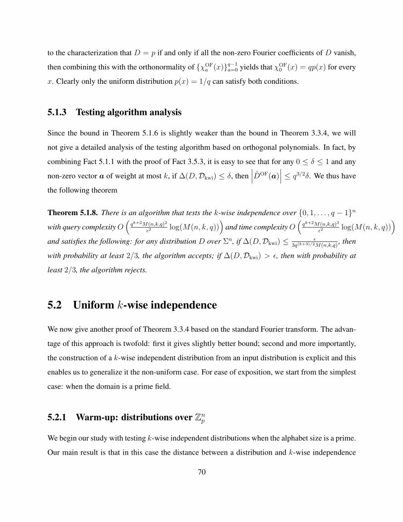
to the characterization that D = p if and only if all the non-zero Fourier coefficients of D vanish,
then combining this with the orthonormality of χOFa (x)q−1
a=0 yields that χOF0 (x) = qp(x) for every
x. Clearly only the uniform distribution p(x) = 1/q can satisfy both conditions.
5.1.3 Testing algorithm analysis
Since the bound in Theorem 5.1.6 is slightly weaker than the bound in Theorem 3.3.4, we will
not give a detailed analysis of the testing algorithm based on orthogonal polynomials. In fact, by
combining Fact 5.1.1 with the proof of Fact 3.5.3, it is easy to see that for any 0 ≤ δ ≤ 1 and any
non-zero vector a of weight at most k, if ∆(D,Dkwi) ≤ δ, then∣∣∣DOF(a)
∣∣∣ ≤ q3/2δ. We thus have
the following theorem
Theorem 5.1.8. There is an algorithm that tests the k-wise independence over 0, 1, . . . , q − 1n
with query complexity O(
qk+2M(n,k,q)2
ε2log(M(n, k, q))
)and time complexity O
(qk+2M(n,k,q)3
ε2log(M(n, k, q))
)and satisfies the following: for any distribution D over Σn, if ∆(D,Dkwi) ≤ ε
3q(k+3)/2M(n,k,q), then
with probability at least 2/3, the algorithm accepts; if ∆(D,Dkwi) > ε, then with probability at
least 2/3, the algorithm rejects.
5.2 Uniform k-wise independence
We now give another proof of Theorem 3.3.4 based on the standard Fourier transform. The advan-
tage of this approach is twofold: first it gives slightly better bound; second and more importantly,
the construction of a k-wise independent distribution from an input distribution is explicit and this
enables us to generalize it the non-uniform case. For ease of exposition, we start from the simplest
case: when the domain is a prime field.
5.2.1 Warm-up: distributions over Znp
We begin our study with testing k-wise independent distributions when the alphabet size is a prime.
Our main result is that in this case the distance between a distribution and k-wise independence
70

can be upper bounded by the sum of the biases (to be defined later) of the distribution, slightly
generalizing an idea of Alon, Goldreich and Mansour [5] that they applied to the binary field case.
Let D be a discrete distribution over Znp , where p is a prime number.
Definition 5.2.1. Let a ∈ Znp be a non-zero vector. We say D is unbiased over a if PD
a,` = 1/p for
every 0 ≤ ` ≤ p−1. The MaxBias(a) of a distribution D is defined to be MaxBiasD(a)def= max0≤j<p PD
a,j−1p.
Note that the MaxBias is non-negative for any distribution. It is well-known that when p is
prime, the Fourier coefficient D(a) of a distribution D over Znp as defined by (2.3) is zero if and
only if Pa,j = 1/p for every 0 ≤ j ≤ p−1. Combining this with the fact that D is unbiased over a
if and only if MaxBiasD(a) is zero, we thus have the following simple characterization of k-wise
independence in terms of MaxBias.
Proposition 5.2.2. D is k-wise independent if and only if for all non-zero a ∈ Znp with wt(a) ≤ k,
MaxBiasD(a) = 0.
We say two non-zero vectors a and b are linearly dependent if there exists some c ∈ Z∗p such
that b = ca and linearly independent if they are not linearly dependent.
Claim 5.2.3. If a and b are linearly dependent, then MaxBiasD(a) = MaxBiasD(b).
Proof. Suppose MaxBiasD(a) is attained at j, i.e., MaxBiasD(a) = Pa,j−1p. Then MaxBiasD(b) ≥
Pb,cj(mod p) −
1p
= Pa,j − 1p
= MaxBiasD(a). Similarly, since c−1 exists, we also have
MaxBiasD(a) ≥ MaxBiasD(b). It follows that MaxBiasD(a) = MaxBiasD(b).
For each a ∈ Znp there are p − 2 other vectors (namely, by taking c = 2, . . . , p − 1) that are
linearly dependent with a.
Lemma 5.2.4. Let a, b ∈ Znp be two non-zero, linearly independent vectors, then for any 0 ≤
ra, rb ≤ p− 1,
Prx∈Zn
p
[n∑
i=1
aixi ≡ ra (mod p) ∧n∑
i=1
bixi ≡ rb (mod p)
]=
1
p2
71

Proof. This follows from the well-known fact that the number of solutions to a system of 2 linearly
independent linear equations over Zp in n variables is pn−2, independent of the vectors of free
coefficients.
Definition 5.2.5 (Strong Orthogonality). Let a and b be two non-zero vectors in Znp . We say
a is strongly orthogonal to b if Ua,j is unbiased over b for every 0 ≤ j ≤ p − 1. That is,
PrX∼Ua,j[b ·X ≡ ` (mod p)] = 1/p, for all 0 ≤ j, ` ≤ p− 1.
Corollary 5.2.6. Let a be a non-zero vector in Znp and b be another non-zero vector that is linearly
independent of a. Then a is strongly orthogonal to b.
Proof. Clearly we have |Sa,j| = pn−1 for all non-zero a and all j. Then by Lemma 5.2.4, the pn−1
points in Sa,j are uniformly distributed over each of the p sets Sb,`, 0 ≤ ` ≤ p− 1.
Now we are ready to prove the following main result of this section.
Theorem 5.2.7. Let D be a distribution over Znp . Then ∆(D,Dkwi) ≤ p
p−1
∑0<wt(a)≤k MaxBiasD(a).
Note that this generalizes the result of [5] for GF(2) to GF(p) for any prime p. When p = 2,
we recover the same (implicit) bound there (our MaxBias is exactly half of their “Bias”).
We first give a brief overview of the proof. We are going to prove Theorem 5.2.7 by construct-
ing a k-wise independent distribution that is close to D. Generalizing the approach in [5], we start
from D, step by step, zeroing-out MaxBiasD(a) for every non-zero vector a of weight at most k.
By Proposition 5.2.2, the resulting distribution will be a k-wise independent one. At each step, we
pick any a with MaxBiasD(a) > 0. To zero-out MaxBiasD(a), we apply a convex combination
between the old distribution and some carefully chosen distribution to get a new distribution. By
the strong orthogonality between linearly independent vectors (c.f. Corollary 5.2.6), if for every
0 ≤ j ≤ q− 1, we mix with D the uniform distribution over all strings in Sa,j with some appropri-
ate weight (this weight can be zero), we will not only zero-out the MaxBias at a but also guarantee
that for any b that is linearly independent from a, MaxBiasD(b) is not going to increase (there-
fore the MaxBias of all zeroed-out vectors will remain zero throughout the correcting steps). This
enables us to repeat the zeroing-out process for all other vectors of weight at most k and finally
obtain a k-wise independent distribution.
72

Proof of Theorem 5.2.7. First we partition all the non-zero vectors of weight at most k into families
of linearly dependent vectors, say F1, F2, . . ., etc. Pick any vector a from F1. If MaxBiasD(a) = 0,
we move on to the next family of vectors. Now suppose MaxBiasD(a) > 0, and without loss of
generality, assume that Pa,0 ≤ Pa,1 ≤ · · · ≤ Pa,p−1. Let εj = Pa,j − 1p. Since
∑p−1j=0 Pa,j = 1, we
have ε0 + · · ·+ εp−1 = 0. Also note that MaxBiasD(a) = εp−1.
Now we define a new distribution D′ as
D′ =1
1 + εD +
εp−1 − ε0
1 + εUa,0 + · · ·+ εp−1 − εp−2
1 + εUa,p−2,
where ε = (εp−1 − ε0) + · · ·+ (εp−1 − εp−2). Now by the triangle inequality,
∆(D, D′) ≤ ε = (εp−1 − ε0) + · · ·+ (εp−1 − εp−2)
= pεp−1 = pMaxBiasD(a).
It is easy to check that MaxBiasD′(a) = 0, since for every 0 ≤ j ≤ p− 1,
PD′
a,j =1
1 + εPD
a,j +εp−1 − εj
1 + ε
=1
1 + ε(PD
a,j + εp−1 − εj)
=1
1 + ε(εp−1 +
1
p)
=1
p(because ε = pεp−1).
Moreover, due to Corollary 5.2.6 and the fact that Ua,j is unbiased over b for every 0 ≤ j < p,
we have for any vector b that is not in the same family with a (i.e., in F2, . . . , etc.),
MaxBiasD′(b) =1
1 + εMaxBiasD(b) ≤ MaxBiasD(b).
In particular, if MaxBiasD(b) is zero, then after zeroing-out the bias at a, MaxBiasD′(b) remains
zero.
Note that once we zero-out the MaxBias over a, then by Claim 5.2.3, the biases over all other
73
p − 2 vectors in F1 vanish as well (that is, we only need to perform one zeroing-out for the p − 1
vectors in the same family). Repeating this process for all other families of vectors, we reach a
distribution Df that is unbiased over all vectors of weight at most k. By Proposition 5.2.2 Df is
k-wise independent and the distance between Df and D is at most as claimed in the theorem.
5.2.2 Distributions over Znq
We now address the main problem of this section, that is, robust characterization of k-wise in-
dependent distributions over domains of the form Znq when q is composite. A straightforward
application of the method for the prime fields case breaks down for general commutative rings
because the strongly orthogonal condition in Corollary 5.2.6 does not hold, even if the two vectors
are linearly independent. Recall that a distribution D over Znq is k-wise independent if and only if
for all non-zero vectors a of weight at most k, D(a) = 0. Our main technical result in this section
is to show, analogous to the prime field case, for a distribution D over the general domain Znq ,
the following holds: for every non-zero vector a of weight at most k, there exists a (small-weight)
distribution such that mixing it with D zeroes-out the Fourier coefficient at a and does not increase
the Fourier coefficient at any other vector.
Unless stated otherwise, all arithmetic operations in this section are performed modulo q; for
instance, we write a = b to mean that ai ≡ bi (mod q) for each 1 ≤ i ≤ n.
Definition 5.2.8 (Prime Vectors). Let a = (a1, . . . , an) be a non-zero vector in Znq . a is called
a prime vector if gcd(a1, . . . , an) = 1. If a is a prime vector, then we refer to the set of vectors
2a, . . . , (q − 1)a (note that all these vectors are distinct) as the multiples of a. A prime vector
and its multiples are collectively referred to as a family of vectors.
Note that families of vectors do not form a partition of the set of all the vectors. For example
when n = 2 and q = 6, vector (4, 0) is a multiple of both (1, 0) and (2, 3), but the latter two are
not multiples of each other. Furthermore, there can be more than one prime vector in a family of
vectors, e.g., for q = 6 again, (2, 3) and (4, 3) are multiples while they are both prime vectors.
Recall that we use Sa,j to denote the set x ∈ Znq :∑n
i=1 aixi ≡ j (mod q).
74

Proposition 5.2.9. If a is a prime vector, then |Sa,j| = qn−1 for any 0 ≤ j ≤ q − 1.
Proof. Since gcd(a1, . . . , an) = 1, there exist integers z1, . . . , zn such that a1z1 + · · ·+ anzn = 1.
Note that for any z ∈ Znq the map hz(x) = x + z is injective. Now if x ∈ Sa,0, then hz(x) =
(x1 + z1, . . . , xn + zn) ∈ Sa,1. Therefore |Sa,0| ≤ |Sa,1|. Similarly we have |Sa,1| ≤ |Sa,2| ≤
· · · ≤ |Sa,q−1| ≤ |Sa,0|. Since the sets Sa,0, . . . , Sa,q−1 form a partition of Znq , it follows that
|Sa,0| = |Sa,1| = · · · = |Sa,q−1| = qn−1.
Linear systems of congruences
A linear system of congruences is a set of linear modular arithmetic equations in some variables.
We will be particularly interested in the case when all modular arithmetic equations are modulo
q. If the number of variables is k, then a solution to the system of congruences is a vector in Zkq .
Two solutions x, x′ in Zkq are congruent to each other if x = x′ (i.e. xi ≡ x′i (mod q) for every
1 ≤ i ≤ k) and incongruent otherwise.
We record some useful results on linear systems of congruences in this section. For more on
this, the interested reader is referred to [35] and [60]. These results will be used in the next section
to show some important orthogonality properties of vectors in Znq . In this section, all matrices are
integer-valued. Let M be a k × n matrix with k ≤ n. The greatest divisor of M is the greatest
common divisor (gcd) of the determinants of all k × k sub-matrices of M . M is a prime matrix if
the greatest divisor of M is 1.
Lemma 5.2.10 ([60]). Let M be a (k + 1) × n matrix. If the sub-matrix consisting of the first k
rows of M is a prime matrix and M has greatest divisor d, then there exist integers u1, . . . , uk such
that for every 1 ≤ j ≤ n,
u1M1,j + u2M2,j + . . . + ukMk,j ≡ Mk+1,j (mod d).
75

Consider the following system of linear congruent equations:M1,1x1 + M1,2x2 + · · ·+ M1,nxn ≡ M1,n+1 (mod q)
......
...
Mk,1x1 + Mk,2x2 + · · ·+ Mk,nxn ≡ Mk,n+1 (mod q).
(5.2)
Let M denote the k × n matrix consisting of the coefficients of the linear system of equations and
let M denote the corresponding augmented matrix of M , that is, the k × (n + 1) matrix with one
extra column consisting of the free coefficients.
Definition 5.2.11. Let M be the coefficient matrix of (5.2) and M be the augmented matrix of M .
Suppose k < n so that system (5.2) is a defective system of equations. Define Yk, Yk−1, . . . , Y1,
respectively, to be the greatest common divisors of the determinants of all the k × k, (k − 1) ×
(k − 1), . . . , 1× 1, respectively, sub-matrices of M . Analogously define Zk, Zk−1, . . . , Z1 for the
augmented matrix M . Also we set Y0 = 1 and Z0 = 1. Finally let s =∏k
j=1 gcd(q,Yj
Yj−1) and
t =∏k
j=1 gcd(q,Zj
Zj−1).
The following Theorem of Smith gives the necessary and sufficient conditions for a system of
congruent equations to have solutions.
Theorem 5.2.12 ([60]). If k < n, then the (defective) linear system of congruences (5.2) has
solutions if and only if s = t. Moreover, if this condition is met, the number of incongruent
solutions is sqn−k.
Weak orthogonality between families of vectors
To generalize the proof idea of the GF(2) case (and also the prime field case studied in Sec-
tion 5.2.1) to commutative rings Zq for arbitrary q, it seems crucial to relax the requirement that
linearly independent vectors are strongly orthogonal. Rather, we introduce the notion of weak
orthogonality between a pair of vectors.
Definition 5.2.13 (Weak Orthogonality). Let a and b be two non-zero vectors in Znq . We say a is
weakly orthogonal to b if for all 0 ≤ j ≤ q − 1, Ua,j(b) = 0.
76

Remark 5.2.14. Note that in general weak orthogonality is not a symmetric relation, that is, a is
weakly orthogonal to b does not necessarily imply that b is weakly orthogonal to a. Also note
that strong orthogonality implies weak orthogonality while the converse is not necessarily true. In
particular, strong orthogonality does not hold in general for linearly independent vectors in Znq .
However, for our purpose of constructing k-wise independent distributions, weak orthogonality
between pairs of vectors suffices.
The following lemma is the basis of our upper bound on the distance between a distribution
and k-wise independence. This lemma enables us to construct a small-weight distribution using
an appropriate convex combination of Ua,jq−1j=0, which on the one hand zeroes-out all the Fourier
coefficients at a and its multiple vectors, on the other hand has zero Fourier coefficient at all other
vectors. The proof of the Lemma 5.2.15 relies crucially on the results in Section 5.2.2 about linear
system of congruences.
Lemma 5.2.15. Let a be a non-zero prime vector and b any non-zero vector that is not a multiple
of a. Then a is weakly orthogonal to b.
Proof. Consider the following system of linear congruences:
a1x1 + a2x2 + · · ·+ anxn ≡ a0 (mod q)
b1x1 + b2x2 + · · ·+ bnxn ≡ b0 (mod q).
(5.3)
Following our previous notation, let M =
a1 a2 · · · an
b1 b2 · · · bn
and M =
a1 a2 · · · an a0
b1 b2 · · · bn b0
.
Since a is a prime vector, Y1 = Z1 = 1. We next show that if b is not a multiple of a, then Y2 can
not be a multiple of q.
Claim 5.2.16. Let a be a prime vector and let M =
a1 a2 · · · an
b1 b2 · · · bn
. The determinants of
all 2×2 sub-matrices of M are congruent to 0 modulo q if and only if a and b are multiple vectors.
Proof. If a and b are multiple vectors, then it is clear that the determinants of all the sub-matrices
are congruent to 0 modulo q. For the only if direction, all we need to prove is that b = ca for some
77

integer c. First suppose that the determinants of all 2× 2 sub-matrices of M are 0. Then it follows
that b1a1
= · · · = bn
an= c. If c is an integer then we are done. If c is not an integer, then c = u
v, where
u, v are integers and gcd(u, v) = 1. But this implies v|ai for every 1 ≤ i ≤ n, contradicting our
assumption that a is a prime vector. Now if not all of the determinants are 0, it must be the case
that the greatest common divisor of the determinants of all 2× 2 sub-matrices, say d′, is a multiple
of q. By Lemma 5.2.10, there is an integer c such that cai ≡ bi (mod d′) for every 1 ≤ i ≤ n.
Consequently, bi ≡ cai (mod q) for every i and hence b is a multiple of a.
Let d = gcd(q, Y2). Clearly 1 ≤ d ≤ q and according to Claim 5.2.16, d 6= q so d|q. Applying
Theorem 5.2.12 with k = 2 to (5.3), the two linear congruences are solvable if and only if d =
gcd(q, Y2) = gcd(q, Z2). If this is the case, the total number of incongruent solutions is dqn−2.
Furthermore, if we let h denote the greatest common divisor of the determinants of all 2 × 2 sub-
matrices of M , then d|h. By Lemma 5.2.10, there is an integer u such that b0 ≡ ua0 (mod h). It
follows that d|(b0 − ua0). Let us consider a fixed a0 and write `0 = ua0 (mod d). Since a is a
prime vector, by Proposition 5.2.9, there are in total qn−1 solutions to (5.3). But for any fixed b0
that has solutions to (5.3), there must be dqn−2 solutions to (5.3) and in addition d|q. Since there
are exactly q/d b0’s in 0, . . . , q − 1, we conclude that (5.3) has solutions for b0 if and only if
b0 = `0 + d`, where `0 is some constant and ` = 0, . . . , qd− 1. Finally we have
Ua,j(b) =∑x∈Zn
q
Ua,j(x)e2πiq
b·x =1
qn−1
∑a·x≡j (mod q)
e2πiq
b·x
=d
q
∑b0:b0=`0+d`
e2πiq
b0 = 0. (by Fact 2.2.2)
This finishes the proof of Lemma 5.2.15.
Correcting the Fourier coefficients of multiple vectors
Now we show how to zero-out a distribution’s Fourier coefficient at every vector in a family. Let D
be a distribution over Znq . By (2.3), for every 1 ≤ ` ≤ q − 1, the Fourier coefficient of a vector `a
can be rewritten as D(`a) =∑q−1
j=0 Pa,je2πiq
`j . Recall that MaxBias(a) = max0≤j≤q−1 Pa,j − 1q.
78

Claim 5.2.17. We have that MaxBias(a) ≤ 1q
∑q−1`=1
∣∣∣D(`a)∣∣∣.
Proof. Since D(`a) =∑q−1
j=0 Pa,je2πiq
`j , by the inverse Fourier transform (2.2), for every 0 ≤ j ≤
q − 1,
Pa,j =1
q
q−1∑`=0
D(`a)e−2πiq
`j.
Since D(0) = 1, we have for every 0 ≤ j ≤ q − 1,
∣∣∣∣Pa,j −1
q
∣∣∣∣ =1
q
∣∣∣∣∣q−1∑`=1
D(`a)e−2πiq
`j
∣∣∣∣∣≤ 1
q
q−1∑`=1
∣∣∣D(`a)e−2πiq
`j∣∣∣ ≤ 1
q
q−1∑`=1
∣∣∣D(`a)∣∣∣ .
Now we are ready to prove the main theorem of this section.
Theorem 3.3.4. Let D be a distribution over Znq , then 3
∆(D,Dkwi) ≤∑
0<wt(a)≤k
∣∣∣D(a)∣∣∣ .
In particular, ∆(D,Dkwi) ≤ M(n, k, q) max0<wt(a)≤k
∣∣∣D(a)∣∣∣ .
Proof. Let a be a prime vector and D(a), D(2a), . . . , D((q − 1)a) be the Fourier coefficients of
a and all the multiples of a. Now construct a new distribution D′ over Znq as
D′ =1
1 + εD +
1
1 + ε
q−1∑j=0
v(j)Ua,j,
where ε =∑q−1
j=0 v(j) and v(j)q−1j=0 are a set of non-negative real numbers that will be specified
later. It is easy to check that D′ is indeed a distribution. Moreover, by Lemma 5.2.15 and linearity
3 It is easy to verify that the same bound holds for prime field case if we transform the bound in MaxBias thereinto a bound in terms of Fourier coefficients. Conversely we can equivalently write the bound of the distance fromk-wise independence in terms of MaxBias at prime vectors. However, we believe that stating the bound in terms ofFourier coefficients is more natural and generalizes more easily.
79

Test-Uniform-KWI(D, k, q, ε)
1. Sample D independently O(
q2M(n,k,q)2
ε2log (M(n, k, q))
)times to obtain
a set Q
2. For every non-zero vector a of weight at most k, use Q to estimate D(a)
3. If maxa
∣∣∣D(a)∣∣∣ ≤ 2ε
3M(n,k,q) , return “Accept”; else return “Reject”
Figure 5-1: Algorithm for testing if a distribution D over Σn is uniform k-wise independent.
of the Fourier transform, for every b that is not a multiple of a,
∣∣∣D′(b)∣∣∣ =
1
1 + ε
∣∣∣D(b)∣∣∣ ≤ ∣∣∣D(b)
∣∣∣ .Without loss of generality, assume that Pa,0 ≤ · · · ≤ Pa,q−1. That is, MaxBias(a) = Pa,q−1 −
1q. If we choose v(j) = Pa,q−1 − Pa,j , then clearly v(j) is non-negative for every 0 ≤ j ≤ q − 1.
Furthermore, by our construction PD′a,j = 1
qfor every j. Therefore by Fact 2.2.1, D′(`a) = 0 for
every 1 ≤ ` ≤ q − 1. Since∑q−1
j=0 Pa,j = 1, it follows that∑q−1
j=0 v(j) = qMaxBias(a). By
Claim 5.2.17,
∆(D, D′) ≤ ε =
q−1∑j=0
v(j) ≤q−1∑`=1
∣∣∣D(`a)∣∣∣ . (5.4)
Finally observe that although some vectors are multiples of more than one prime vector (thus
they belong to more than one family and appear more than once in (5.4)), because the distance
bound in (5.4) is the sum of magnitudes of all the Fourier coefficients in the family, once a vector’s
Fourier coefficient is zeroed-out, it will not contribute to the distance bound at any later stage. This
completes the proof of the theorem.
Testing algorithm and its analysis
We are now ready to prove the following result on testing k-wise independence over Znq .
Theorem 5.2.18. There is an algorithm that tests the k-wise independence over Σn with query
complexity O(n2k(q−1)2kq2
ε2) and time complexity O(n3k(q−1)3kq2
ε2) and satisfies the following: for
80

any distribution D over Σn, if ∆(D,Dkwi) ≤ ε3qM(n,k,q)
, then with probability at least 2/3, the
algorithm accepts; if ∆(D,Dkwi) > ε, then with probability at least 2/3, the algorithm rejects.
Proof. Our testing algorithm simply plugs the upper bound on distance to k-wise independence
in Theorem 3.3.4 into the Generic Algorithm as shown in Fig. 3-1. The algorithm is described in
Figure 5-1. For the analysis of Test-Uniform-KWI(D, k, q, ε), we simply apply Theorem 3.5.2
with K = M(n, k, q), A = a ∈ Σn : 0 < wt(a) ≤ k and κ = q. To see κ = q, note that
Pa,j = 1/q holds for every a in A and 0 ≤ j ≤ q−1 for any k-wise independent distribution. Since
no (randomized) algorithm can increase the statistical difference between two distributions [58], by
Fact 3.5.3 (more precisely, the proof of Fact 3.5.3), if ∆(D,Dkwi) ≤ δ, then we have∣∣∣D(a)
∣∣∣ ≤ qδ
for every a ∈ A.
5.2.3 Distributions over product spaces
Now we generalize the underlying domains from Znq to product spaces. Let Σ1, . . . , Σn be n
finite sets. Without loss of generality, let Σi = 0, 1, . . . , qi − 1. In this section, we consider
distributions over the product space Ω = Σ1 × · · · × Σn. For a set of integers q1, . . . , qn, denote
their least common multiple (lcm) by lcm(q1, . . . , qn). Let Qdef=lcm(q1, . . . , qn) and in addition, for
every 1 ≤ i ≤ n, set Mi = Qqi
. Then we can rewrite the Fourier coefficient defined in (2.1) as
D(a) =∑
x∈Σ1×···×Σn
D(x)e2πiQ
(M1a1x1+···+Mnanxn)
=∑
x∈Σ1×···×Σn
D(x)e2πiQ
(a′1x1+···+a′nxn),
where a′i ≡ Miai (mod Q) for every 1 ≤ i ≤ n. This suggests that we may view D as a distribution
over Σn with effective alphabet size |Σ| = Q = lcm(q1, . . . , qn) and consider the following map
from vectors in Σ1 × · · · × Σn to vectors in ZnQ:
H : (a1, . . . , an) 7→ (M1a1 (mod Q), . . . ,Mnan (mod Q)) . (5.5)
Then we only need to consider the Fourier coefficients at vectors a′def=H(a) = (a′1, . . . , a
′n) ∈
81

ZnQ (that is, vectors in Zn
Q whose ith component is a multiple of Mi for every i). Note that in general
M = lcm(q1, . . . , qn) could be an exponentially large number and is therefore not easy to handle in
practice4. However, this difficulty can be overcome by observing the following simple fact. Since
we are only concerned with vectors of weight at most k, we may take different effective alphabet
sizes for different index subsets of size k. For example, consider a k-subset S = i1, . . . , ik. Then
the effective alphabet size of S is |ΣS| = lcm(qi1 , . . . , qik), which is at most poly(n) if we assume
k is a constant and each qi is polynomially bounded.
Our main result for distributions over product spaces is the following theorem.
Theorem 5.2.19. Let D be a distribution over Σ1×· · ·×Σn. Then ∆(D,Dkwi) ≤∑
0<wt(a)≤k
∣∣∣D(a)∣∣∣ .
We now sketch the proof of Theorem 5.2.19.
A vector a ∈ Σ1×· · ·×Σn is a prime vector if gcd(a1, . . . , an) = 1. For any integer ` > 0, the
`-multiple of a is `adef=(`a1 (mod q1), . . . , `an (mod qn)). Let a be a prime vector. Then vectors
in the set 2a, . . . , (Q − 1)a are called the multiple vectors of a. Note that these Q − 1 vectors
may not be all distinct.
The main difficulty in applying our result for distributions over Znq to distributions over product
spaces is that the mapping in (5.5) is not surjective. In particular, after the mapping some families
of vectors may have no prime vector in it. To handle this problem, we slightly generalize the result
of weak orthogonality in Lemma 5.2.15 to non-prime vectors. Specifically, we say a non-zero
vector a (not necessarily prime) is weakly orthogonal to vector b if Ua,`(b) = 0 for all ` such that
Sa,` is non-empty.
Lemma 5.2.20. Let a and b be two vectors in Znq . If b is not a multiple of a, then vector a is
weakly orthogonal to b.
Proof. Clearly we only need to prove the case when a is not a prime vector. Let a be any prime
vector that is a multiple of a and suppose a = da. Now Sa,` is non-empty only if ` ≡ `′d (mod q)
for some integer `′. Note that Sa,`′d = ∪j:jd≡`′d (mod q)Sa,j . Since the sets Sa,jq−1
j=0 are pairwise
4Recall that the testing algorithm requires estimating all the low-degree Fourier coefficients, where each Fouriercoefficient is an exponential sum with M as the denominator.
82
disjoint, it follows that Ua,`′d = 1gcd(d,q)
∑j:jd≡`′d (mod q) Ua,j , where gcd(d, q) is the number of
incongruent j’s satisfying jd ≡ `′d (mod q). Now by Lemma 5.2.15, if b is not a multiple of a,
then Ua,j(b) = 0 for every j. It follows that Ua,`d(b) = 0.
Note that for any integer ` > 0 and every 1 ≤ i ≤ n, `ai ≡ bi (mod qi) if and only if
`aimi ≡ bimi (mod Q), hence the map H preserves the multiple relationship between vectors.
Now Lemma 5.2.20 implies that if we map the vectors in Σ1 × · · · × Σn to vectors in ZnQ as
defined in (5.5), then we can perform the same zeroing-out process as before: for each family of
vectors, zero-out all the Fourier coefficients at the vectors in this family using a mixture of uniform
distributions without increasing the magnitudes of the Fourier coefficients everywhere else. This
will end up with a k-wise independent distribution over the product space Σ1 × · · · × Σn.
Next we bound the total weight required to zero-out a family of vectors. Let S be any k-subset
of [n]. Without loss of generality, we may take S = [k]. Let qS = lcm(q1, . . . , qk) and let mi = qS
qi
for each 1 ≤ i ≤ k. Let a ∈ Σ1 × · · · × Σn be a prime vector whose support is contained in [k].
Then
D(a) =∑
x∈Σ1×···×Σk
DS(x)e2πi(
a1x1q1
+···+akxkqk
)
=∑
x∈Σ1×···×Σk
DS(x)e2πiqS
(m1a1x1+···+mkakxk)
=∑
x∈Σ1×···×Σk
DS(x)e2πiqS
(a′1x1+···+a′kxk),
where, as before, we define a′ = (a′1, . . . , a′k) with a′i = miai (mod qS) for 1 ≤ i ≤ k.
Let d = gcd(m1a1 (mod qS), . . . ,mkak (mod qS)) = gcd(a′1, . . . , a′k) and set Sa′,j = x ∈
Σ1 × · · · × Σk : a′1x1 + · · ·+ a′kxk ≡ j (mod qS). Clearly Sa′,j is non-empty only if d|j.
Claim 5.2.21. Let a be a vector in Σ1×· · ·×Σk with d = gcd(a′1, . . . , a′k). Then |Sa′,`d| = dq1···qk
qS
for every 0 ≤ ` ≤ qS
d− 1.
Proof. Since d = gcd(a′1, . . . , a′k), if we let bi =
a′id
for each 1 ≤ i ≤ k, then gcd(b1, . . . , bk) = 1.
Now applying the same argument as in the proof of Proposition 5.2.9 gives the desired result.
83

Now for every 1 ≤ ` ≤ qS
d− 1 and put q∗
def= qS
d, we have
D(`a) =∑
x∈Σ1×···×Σk
DS(x)e2πi(
`a1x1q1
+···+ `akxkqk
)
=∑
x∈Σ1×···×Σk
DS(x)e2πiqS
`a′·x=
qSd−1∑
j=0
PrX∼D
[a′ ·X ≡ jd (mod qS)]e2πiqS
`jd
=
qSd−1∑
j=0
w(j)e2πiqS
`jd=
q∗−1∑j=0
w(j)e2πiq∗ `j,
where w(j)def=Pa′,jd. That is, each of the Fourier coefficients D(a), D(2a), . . . , D((q∗ − 1)a) can
be written as a one-dimensional Fourier transform of a function (namely, w(j)) over Zq∗ . Then
following the same proofs as those in Sec. 5.2.2, we have that the total weight to zero-out the
Fourier coefficients at a and its multiples is at most∑ qS
d−1
`=1
∣∣∣D(`a)∣∣∣. This in turn gives the upper
bound stated in Theorem 5.2.19 on the distance between D and k-wise independence over product
spaces.
Testing algorithm and its analysis
We study the problem of testing k-wise independence over the product space Σ1× · · ·×Σn in this
section.
To simplify notation, in the following we write
Mprod =k∑
`=1
∑I∈([n]
` )
∏i∈I
(qi − 1)
for the total number of non-zero Fourier coefficients of weight at most k, and
qmax = maxS∈([n]
k )lcm(qi : i ∈ S)
for the maximum effective alphabet size of any index subset of size k.
84

Test-Product-KWI(D, k, q, ε)
1. Sample D independently O(
q2maxMprod(n,k,q)2
ε2log(Mprod(n, k, q)
))times to ob-
tain a set Q
2. For every non-zero vector a of weight at most k, use Q to estimate D(a)
3. If maxa
∣∣∣D(a)∣∣∣ ≤ 2ε
3Mprod(n,k,q), return “Accept”; else return “Reject”
Figure 5-2: Algorithm for testing uniform k-wise independence over product spaces.
Note that a simple corollary of Theorem 5.2.19 is
∆(D,Dkwi) ≤ Mprod max0<wt(a)≤k
∣∣∣D(a)∣∣∣ ,
which gives the soundness condition for the distance bound. For the completeness condition,
it is easy to see that for any 0 ≤ δ ≤ 1 and any non-zero vector a of weight at most k, if
∆(D,Dkwi) ≤ δ, then∣∣∣D(a)
∣∣∣ ≤ qmaxδ. The following theorem can now be proved easily by
plugging these two conditions into Theorem 3.5.2. We omit the proof.
Theorem 5.2.22. There is an algorithm that tests the k-wise independence over the product space
Σ1×· · ·×Σn (as shown in Fig 5-2) with query complexity O(
q2maxMprod(n,k,q)2
ε2log(Mprod(n, k, q)
))and time complexity O
(q2maxMprod(n,k,q)3
ε2log(Mprod(n, k, q)
))and satisfies the following: for any
distribution D over Σn, if ∆(D,Dkwi) ≤ ε3qmaxMprod(n,k,q)
, then with probability at least 2/3, the
algorithm accepts; if ∆(D,Dkwi) > ε, then with probability at least 2/3, the algorithm rejects.
85

86

Chapter 6
Non-uniform k-wise Independence
In this chapter we seek a robust characterization of non-uniform k-wise independent distributions.
For ease of exposition, we present our results only for the case when the underlying domain is
0, 1, . . . , q − 1n. Our approach can be generalized easily to handle distributions over product
spaces. The chapter is organized as follows. First we introduce non-uniform Fourier coefficients in
Section 6.1. A new characterization of non-uniform k-wise independence based on non-uniform
Fourier coefficients is present in Section 6.2. Next, in Section 6.3, we demonstrate how to zero-out
all the low-level non-uniform Fourier coefficients step by step. In Section 6.4 we study the testing
algorithm of non-uniform k-wise independence. Finally, we consider the problem of testing non-
uniform k-wise independence when the marginal probabilities are unknown in Section 6.5.
Recall that a distribution D : Σn → [0, 1] is k-wise independent if for any index subset
S ⊂ [n] of size k, S = i1, . . . , ik, and for any z1 · · · zk ∈ Σk, DS(z1 · · · zk) = PrD[Xi1 =
z1] · · ·PrD[Xik = zk]. Our strategy of showing an upper bound on the distance between D and
non-uniform k-wise independence is to reduce the non-uniform problem to the uniform case and
then apply Theorem 3.3.4.
87

6.1 Non-uniform Fourier coefficients
In the following we define a set of factors which are used to transform non-uniform k-wise inde-
pendent distributions into uniform ones. Let pi(z)def= PrD[Xi = z]. We assume that 0 < pi(z) < 1
for every i ∈ [n] and every z ∈ Σ (this is without loss of generality since if some pi(z)’s are
zero, then it reduces to the case of distributions over product spaces). Let θi(z)def= 1
qpi(z). Intuitively,
one may think of the θi(z)’s as a set of compressing/stretching factors which transform a non-
uniform k-wise distribution into a uniform one. For convenience of notation, if S = i1, . . . , i`
and z = zi1 · · · zi` , we write θS(z) for the product θi1(zi1) · · · θi`(zi`).
Definition 6.1.1 (Non-uniform Fourier Coefficients). Let D be a distribution over Σn. Let a
be a non-zero vector in Σn and supp(a) to be its support. Let Dsupp(a) be the projection of
D to coordinates in supp(a). For every z in the support of Dsupp(a), define D′supp(a)(z) =
θsupp(a)(z)Dsupp(a)(z), which is the transformed distribution1 of the projected distribution Dsupp(a).
The non-uniform Fourier coefficient of D at a, denoted Dnon(a), is defined by
Dnon(a)def=D′supp(a)(a) =
∑z∈Σ|supp(a)|
D′supp(a)(z)e2πiq
a·z. (6.1)
Remark 6.1.2. In the following we always refer to Dnon collectively as a set of (complex) num-
bers that will be used to indicate the distance between distribution D and the non-uniform k-wise
independence. Strictly speaking, Dnon are not Fourier coefficients since in general there is no
distribution whose (low degree) Fourier coefficients are exactly Dnon.
To summarize, let us define a function
F : (R≥0)Σn × (
([n]
k
)× Σk) → (R≥0)Σk
which maps a distribution D over Σn and a vector a ∈ Σn of weight k to a non-negative function
1Note that in general D′supp(a) is not a distribution: it is non-negative everywhere but
∑x D′
supp(a)(x) = 1 maynot hold.
88

over Σ|supp(a)|. That is, for every z ∈ Σk,
F(D, a)(z) = Dsupp(a)(z)θsupp(a)(z). (6.2)
Then the non-uniform Fourier coefficient of D at a is simply the ordinary uniform Fourier coeffi-
cient of F(D, a) at a:
Dnon(a) = F(D, a)(a).
The idea of defining D′supp(a) is that if D is non-uniform k-wise independent, then D′supp(a) will
be a uniform distribution over the coordinates in supp(a). Indeed, our main result in this section
is to show a connection between the non-uniform Fourier coefficients of D and the property that
distribution D is non-uniform k-wise independent. In particular we have the following simple
characterization of the non-uniform k-wise independence.
Theorem 6.1.3. A distribution D over Σn is non-uniform k-wise independent if and only if for
every non-zero vector a ∈ Σn of weight at most k, Dnon(a) = 0.
6.2 New characterization of non-uniform k-wise independence
We prove Theorem 6.1.3 in this section. It is straightforward to show that if D is a non-uniform k-
wise independent distribution, then all the non-zero non-uniform Fourier coefficients of degree at
most k are zero. However, the proof of the converse is more involved. The key observation is that
if we write the non-uniform Fourier transform as a linear transformation, the non-uniform Fourier
transform matrix, like the uniform Fourier transform matrix, can be expressed as a tensor product
of a set of heterogeneous DFT (discrete Fourier transform) matrices (as opposed to homogeneous
DFT matrices in the uniform case). This enables us to show that the non-uniform Fourier transform
is invertible. Combined with the condition that all the non-trivial non-uniform Fourier coefficients
are zero, this invertibility property implies that D must be a non-uniform k-wise independent
distribution.
Recall that our new characterization of non-uniform k-wise independent distributions is:
89

Theorem 6.1.3. A distribution D over Σn is k-wise independent if and only if for every non-zero
vector a ∈ Σk with wt(a) ≤ k, Dnon(a) = 0.
Proof. Suppose D is a non-uniform k-wise independent distribution. Then it is easy to see that for
any non-empty T ⊂ [n] of size at most k (not just for subsets whose sizes are exactly k),
DT (zT ) =∏i∈T
pi(zi).
Indeed, if |T | = k then this follows directly from the definition of non-uniform k-wise independent
distributions. If |T | < k, let S ⊃ T be any index set of size k, then
DT (zT ) =∑
zj :j∈S\T
DS(zS)
=∑
zj :j∈S\T
∏`∈S
p`(z`)
=∏i∈T
pi(zi)∑
zj :j∈S\T
∏j∈S\T
pj(zj)
=∏i∈T
pi(zi)∏
j∈S\T
∑zj∈Σ
pj(zj)
=∏i∈T
pi(zi),
as∑
zj∈Σ pj(zj) = 1 for every 1 ≤ j ≤ n.
Let a be any non-zero vector of weight ` ≤ k whose support set is supp(a). Now we show that
D′supp(a) is a uniform distribution and consequently all the non-uniform Fourier coefficients whose
support sets are supp(a) must be zero. Indeed, by the definition of D′,
D′supp(a)(zsupp(a)) = Dsupp(a)(zsupp(a))∏
i∈supp(a)
θi(zi)
=∏
i∈supp(a)
pi(zi)∏
i∈supp(a)
1
qpi(zi)
=1
q`
90

for every zsupp(a) ∈ 0, 1, . . . , q − 1`. Hence Dnon(a) = D′supp(a)(a) = 0 by Theorem 2.2.4.
The converse direction will follow directly from Lemma 6.2.1 below by setting E = DS in the
statement.
Lemma 6.2.1. Let E : Σk → R≥0 be a distribution. For any index set T ⊆ [k], let ET (z),
E ′T (z) and Enon(a) be defined analogously to those of DT (z), D′T (z) and Dnon(a), respectively.
If Enon(a) = 0 for every non-zero vector a, then E is a non-uniform independent distribution, i.e.
E ′[k] is the uniform distribution and consequently E is a product distribution.
One may think of Lemma 6.2.1 as the non-uniform version of Proposition 2.2.3.
Proof. For notational simplicity we write S = [k]. Let T be a subset of S of size k − 1, and
without loss of generality, we assume that T = 1, . . . , k − 1. We first observe the following
relation between E ′S(z) and E ′T (zT ).
E ′T (z1, . . . , zk−1) = ET (z1, . . . , zk−1)θ1(z1) · · · θk−1(zk−1)
=∑zk
ES(z1, . . . , zk−1, zk)θ1(z1) · · · θk−1(zk−1)
=∑zk
1
θk(zk)E ′S(z1, . . . , zk)
=∑zk
qpk(zk)E′S(z1, . . . , zk).
By induction, we have in general, for any T ⊂ S,
E ′T (zT ) =∑
zj :j∈S\T
E ′S(z1, . . . , zk)∏
j∈S\T
(qpj(zj)). (6.3)
Next we use (6.3) to eliminate the intermediate projection distributions E ′T , and write the non-
uniform Fourier transform of E as a linear transform of E ′S(z)z∈Σk . Let a be a vector whose
support set is T , then
Enon(a) = E ′T (a)
91

=∑
zi:i∈T
E ′T (zT )e2πiq
Pi∈T aizi
=∑
zi:i∈T
∑zj :j∈S\T
E ′S(z)e2πiq
Pi∈T aizi
∏j∈S\T
(qpj(zj))
=∑z∈Σk
E ′S(z)∏i∈T
e2πiq
aizi∏
j∈S\T
(qpj(zj))
=∑z∈Σk
E ′S(z)∏
i∈supp(a)
e2πiq
aizi∏
j∈S\supp(a)
(qpj(zj)). (6.4)
Define a qk-dimensional column vector E′ with entries E ′S(z) (we will specify the order of
the entries later). Similarly define another qk-dimensional column vector whose entries are the
non-uniform Fourier coefficients Enon. Then we may write (6.4) more compactly as
Enon = FE′. (6.5)
In what follows, we will show that F can be written nicely as a tensor product of k matrices. This
in turn enables us to show that F is non-singular.
Let ω = e2πiq be a primitive qth root of unity. The q-point discrete Fourier transform (DFT)
matrix is given by
F =
1 1 1 1 · · · 1
1 ω ω2 ω3 · · · ωq−1
1 ω2 ω4 ω6 · · · ω2(q−1)
1 ω3 ω6 ω9 · · · ω3(q−1)
......
......
...
1 ωq−1 ω2(q−1) ω3(q−1) · · · ω(q−1)(q−1)
Note that a DFT matrix is also a Vandermonde matrix and therefore det(F) 6= 0.
Definition 6.2.2 (Tensor Product of Vectors and Matrices). Let A be an m × n matrix and B be
a p × q matrix. Then the tensor product (a.k.a. Kronecker product) A ⊗ B is an mp × nq block
92

matrix given by
A⊗B =
a00B · · · a0,n−1B
... . . . ...
am−1,0B · · · am−1,n−1B
=
a00b00 · · · a00b0,q−1 · · · · · · a0,n−1b00 · · · a0,n−1b0,q−1
... . . . ...... . . . ...
a00bp−1,0 · · · a00bp−1,q−1 · · · · · · a0,n−1bp−1,0 · · · a0,n−1bp−1,q−1
...... . . . ...
......
... . . . ......
am−1,0b00 · · · am−1,0b0,q−1 · · · · · · am−1,n−1b00 · · · am−1,n−1bp−1,q−1
... . . . ...... . . . ...
am−1,0bp−1,0 · · · am−1,0bp−1,q−1 · · · · · · am−1,n−1bp−1,0 · · · am−1,n−1bp−1,q−1
.
Let a be an m-dimensional column vector in Rm and b be a p-dimensional column vector in Rp.
Then the tensor product a⊗b is an mp-dimensional column vector in Rmp and its entries are given
by
a⊗ b =
a0
...
am−1
⊗
b0
...
bp−1
=
a0b0
...
a0bp−1
...
...
am−1b0
...
am−1bp−1
.
Let q ≥ 2 be an integer. The q-ary representation of a natural number r is an ordered tuple
(bk, . . . , b1, b0) such that 0 ≤ bi ≤ q − 1 for every 0 ≤ i ≤ k and r = b0 + b1 · q + · · · bk · qk.
The following simple while useful fact about the tensor product of matrices can be proved easily
by induction on the number of matrices in the product.
93

Fact 6.2.3. Let F (1), . . . , F (k) be a set of q × q matrices where the (i, j)th entry of F (`) is denoted
by F(`)i,j , 0 ≤ i, j ≤ q − 1. Let G = F (1) ⊗ · · · ⊗ F (k). For 0 ≤ I, J ≤ qk − 1, let the q-ary
representations of I and J be I = (i1, . . . , ik) and J = (j1, . . . , jk), respectively. Then
GI,J = F(1)i1,j1
· · ·F (k)ik,jk
.
Let’s first consider the simple case when E is a one-dimensional distribution. Let E be the
column vector whose entries are values of E at 0, 1, . . . , q − 1. Similarly let E be the column
vector of E’s Fourier transform. If we arrange the entries of E and E in increasing order, then the
one-dimensional (uniform) Fourier transform can be written in the matrix multiplication form as
E =
E(0)
...
E(q − 1)
= F
E(0)
...
E(q − 1)
= FE. (6.6)
For the general case in which E is a distribution over 0, 1, . . . , q − 1k, we may view every
k-dimensional point (x1, . . . , xk) in E(x1, . . . , xk) as the representation of a natural number X in
the q-ary representation: X = x1 · qk−1 + · · · + xk−1 · q + xk. Then this provides a natural order
of the entries in any column vector defined over 0, 1, . . . , q − 1k: view each vector (x1, . . . , xk)
as a natural number X in the q-ary representation and arrange them in the increasing order. By
tensor product and arranging the entries in E and E in the natural order, the k-dimensional Fourier
transform can be written as
E =
E(0, 0, . . . , 0)
...
E(q − 1, q − 1, . . . , q − 1)
= F⊗ · · · ⊗ F︸ ︷︷ ︸k times
E(0, 0, . . . , 0)
...
E(q − 1, q − 1, . . . , q − 1)
=
F⊗ · · · ⊗ F︸ ︷︷ ︸k times
E.
(6.7)
Definition 6.2.4 (Non-uniform DFT Matrices). For every 1 ≤ i ≤ k, define (recall that pi(z)’s are
94

the marginal probabilities of E at coordinate i) the non-uniform DFT matrix at coordinate i to be
Fi =
qpi(0) qpi(1) qpi(2) qpi(3) · · · qpi(q − 1)
1 ω ω2 ω3 · · · ωq−1
1 ω2 ω4 ω6 · · · ω2(q−1)
1 ω3 ω6 ω9 · · · ω3(q−1)
......
......
...
1 ωq−1 ω2(q−1) ω3(q−1) · · · ω(q−1)(q−1)
The following lemma follows directly from Fact 6.2.3 and (6.4).
Lemma 6.2.5. If we arrange the entries in E′ and Enon in the natural order, then the qk×qk matrix
F in (6.5) is the tensor product of k non-uniform DFT matrices, i.e.,
F = F1 ⊗ · · · ⊗ Fk,
and consequently
Enon = (F1 ⊗ · · · ⊗ Fk)E′.
The following is a well-known fact on the determinants of tensor product matrices, see e.g. [59]
for an elementary proof.
Fact 6.2.6. If A is an m×m square matrix and B is an n× n square matrix, then
det(A⊗B) = (det(A))n(det(B))m.
Proposition 6.2.7. The non-uniform DFT matrix is non-singular for every 1 ≤ i ≤ k. In particu-
lar,
det(Fi) = q (pi(0) + · · ·+ pi(q − 1)) (−1)q−1∏
1≤`<m≤q−1
(ωm−ω`) = (−1)q−1q∏
1≤`<m≤q−1
(ωm−ω`) 6= 0.
95
Proof. By Laplace expansion along the first row, we have
det(Fi) =
q−1∑j=0
(−1)jqpi(j) det(M1j). (6.8)
The determinant of the minor M1j is
det(M1j) =
∣∣∣∣∣∣∣∣∣∣∣∣
1 ω · · · ωj−1 ωj+1 · · · ωq−1
1 ω2 · · · ω2(j−1) ω2(j+1) · · · ω2(q−1)
......
......
... . . . ...
1 ωq−1 · · · ω(j−1)(q−1) ω(j+1)(q−1) · · · ω(q−1)(q−1)
∣∣∣∣∣∣∣∣∣∣∣∣
=
(q−1∏
`=0,` 6=j
ω`
)∣∣∣∣∣∣∣∣∣∣∣∣
1 1 · · · 1 1 · · · 1
1 ω · · · ωj−1 ωj+1 · · · ωq−1
......
......
... . . . ...
1 ωq−2 · · · ω(j−1)(q−2) ω(j+1)(q−2) · · · ω(q−1)(q−2)
∣∣∣∣∣∣∣∣∣∣∣∣=
q−1∏`=0,` 6=j
ω`∏
0≤`<m≤q−1`,m6=j
(ωm − ω`)
=
∏q−1`=0,` 6=j ω`
∏0≤`<m≤q−1(ω
m − ω`)∏j−1`=0(ω
j − ω`)∏q−1
`=j+1(ω` − ωj)
,
since the matrix in the second step is a Vandermonde matrix.
Using the fact that ωq = 1, the denominator may be simplified as
j−1∏`=0
(ωj − ω`)
q−1∏`=j+1
(ω` − ωj)
=(−1)j
j−1∏`=0
ω`
j∏`=1
(1− ω`)
q−1∏`=j+1
(ω` − ωj)
=(−1)j
j−1∏`=0
ω`
j∏`=1
(1− ω`)
q−1∏`=j+1
ω`−q(ωq − ωq+j−`)
96

=(−1)j
j−1∏`=0
ω`
j∏`=1
(1− ω`)
q−1∏`=j+1
ω`
q−1∏`=j+1
(1− ωq+j−`)
=(−1)j
q−1∏`=0,` 6=j
ω`
q−1∏`=1
(1− ω`).
Therefore we have
det(M1j) = (−1)j(−1)q−1∏
1≤`<m≤q−1
(ωm − ω`).
Plugging det(M1j) into (6.8) completes the proof.
Combining Fact 6.2.6 and Proposition 6.2.7 gives
Lemma 6.2.8. We have that
det(F) = det(F1 ⊗ · · · ⊗ Fk) 6= 0.
Recall that we assume that all the non-zero Fourier coefficients Enon(a) are zero. Now to
make the linear system of equations in (6.5) complete, we add another constraint that Enon(0) =∑z E ′(z) = cqk, where c is a constant which will be determined later. Since F is non-singular,
there is a unique solution to this system of qk linear equations. But we know the uniform dis-
tribution E ′(z) = c for every z ∈ Σk is a solution (by the proof of the only if direction of
Theorem 6.1.3), therefore this is the unique solution.
Now we have, for every z ∈ Σk, E(z)θS(z) = c. Observe that 1/θS(z) = qkp1(z1) · · · pk(zk),
and since pi(z)’s are marginal probabilities,∑
z∈Σ pi(z) = 1 for every i, it follows that
∑z∈Σk
1
θS(z)= qk
∑z∈Σk
p1(z1) · · · pk(zk) = qk.
Using the fact that∑
z∈Σk E(z) = 1, we arrive at
1 =∑z∈Σk
E(z) = c∑z∈Σk
1
θS(z)= qkc,
97
and therefore c = 1qk and E(z) = 1
qkθS(z)= p1(z1) · · · pk(zk) as desired. This completes the proof
of Lemma 6.2.1.
6.3 Zeroing-out non-uniform Fourier coefficients
Given a distribution D which is not k-wise independent, what is the distance between D and the
non-uniform k-wise independence? In the following we will, based on the approach that has been
applied to the uniform case, try to find a set of small-weight distributions to mix with D in order
to zero-out all the non-uniform Fourier coefficients of weight at most k. Moreover, we can bound
the total weight added to the original distribution in this zeroing-out process in terms of the non-
uniform Fourier coefficients of D. This will show that the characterization of the non-uniform
k-wise independence given in Theorem 6.1.3 is robust.
A careful inspection of Theorem 3.3.4 and its proof shows that if we focus on the weights
added to correct any fixed prime vector and its multiples, we actually prove the following.
Theorem 6.3.1. Let E ′ be a non-negative function2 defined over Σn, a be a prime vector of weight
at most k and E ′(a), E ′(2a), . . . , E ′((q − 1)a) be the Fourier coefficients at a and its multiple
vectors. Then there exist a set of non-negative real numbers wj, j = 0, 1, . . . , q − 1, such that the
(small-weight) distribution3 WE′,adef=∑q−1
j=0 wjUa,j satisfies the following properties. The Fourier
coefficients of E ′ + WE′,a at a, 2a, . . . , (q − 1)a all equal zero and WE′,a(b) = 0 for all non-zero
vectors that are not multiples of a. Moreover, the total weight of WE′,a is at most∑q−1
j=0 wj ≤∑q−1`=1
∣∣∣E ′(`a)∣∣∣.
Applying Theorem 6.3.1 with E ′ equal to D′supp(a) gives rise to a small-weight distribution
WD′supp(a)
,a which, by abuse of notation, we denote by Wa. When we add Wa to D′supp(a), the
resulting non-negative function has zero Fourier coefficients at a and all its multiple vectors. That
2In Theorem 3.3.4 we only prove this for the case when E′ is a distribution. However it is easy to see that the resultapplies to non-negative functions as well.
3Recall that Ua,j is the uniform distribution over all strings x ∈ Znq such that a · x ≡ j (mod q).
98

is,
Wa(`a) = −D′supp(a)(`a), for every 1 ≤ ` ≤ q − 1. (6.9)
= −Dnon(`′a), for every `′ such that supp(`′a) = supp(a). (6.9′)
and for any b which is not a multiple of a,
Wa(b) = 0. (6.10)
However, this small-weight distribution only works for the auxiliary function D′supp(a) but what
we are looking for is a small-weight distribution that corrects the non-uniform Fourier coefficients
of D at a. To this end, we apply the reversed compressing/stretching factor to Wa to get Wa,
Wa(x)def=
Wa(x)
θ[n](x). (6.11)
The following lemma shows that mixing D with Wa results in a distribution whose non-uniform
Fourier coefficients at a as well as its multiple vectors are zero4. In addition, the mixing only adds
a relatively small weight and may increase the magnitudes of the non-uniform Fourier coefficients
only at vectors whose supports are completely contained in the support of a.
Lemma 6.3.2. Let D be a distribution over Σn and a be a prime vector of weight at most k. Let
supp(a) be the support set of a and Wa be as defined in (6.11). Let the maximum factor over all
possible compressing/stretching factors be denoted as γkdef= maxS,z
1θS(z)
, where S ranges over all
subsets of [n] of size at most k and z ∈ Σ|S|. Then Wa satisfies the following properties:
1. The non-uniform Fourier coefficients of D + Wa at a as well as at the multiple vectors of a
whose support sets are also supp(a) are all zero.5 Moreover, ˆW nona (a′) = 0 for every vector
a′ whose support set is supp(a) but is not a multiple vector of a.
4In fact, the lemma only guarantees to zero-out the Fourier coefficients at a and its multiples whose support setsare the same as that of a. But that will not be a problem since we will perform the correction process in stages andwill come to vectors with smaller support sets at some later stages.
5Note that if a is a prime vector and a′ is a multiple vector of a, then supp(a′) ⊆ supp(a).
99

2. For any vector b with supp(b) * supp(a), ˆW nona (b) = 0.
3. The total weight of Wa is at most γk
∑x∈Σn Wa(x) ≤ γk
∑q−1j=1
∣∣∣Dnon(ja)∣∣∣.
4. For any non-zero vector c with supp(c) ⊂ supp(a), ˆW nona (c) ≤ γk
∑q−1j=1
∣∣∣Dnon(ja)∣∣∣.
Proof. For simplicity, we assume that supp(a) = [k]. Recall that Wa =∑q−1
j=0 wjUa,j and Ua,j
is the uniform distribution over the strings x ∈ Znq such that
∑ni=1 aixi ≡ j (mod q). A simple
while important observation is the following: since the support of a is [k], if x1 · · ·xk satisfies
the constraint∑k
i=1 aixi ≡ j (mod q), then for any yk+1 · · · yn ∈ Σn−k, x1 · · ·xkyk+1 · · · yn will
satisfy the constraint and thus is in the support of the distribution.
Remark on notation. In the rest of this section, we always write x for an n-bit vector in Σn and
write z for a k-bit vector in Σk.
Note that we may decompose Wa (or any non-negative function) into a sum of qk weighted
distributions as Wa =∑
z∈Σk wzUz, such that each of the distribution Uz is supported on the
|Σ|n−k strings whose k-bit prefixes are z. That is,
wzUz(x) =
Wa(x), if x[k] = z,
0, otherwise.
To make Uz indeed a distribution, i.e.,∑
x Uz(x) = 1, we simply set
wzdef= (Wa)[k] (z). (6.12)
That is, wz equals the mass of the projected distribution Wa at z. By Theorem 6.3.1 clearly we
have ∑z∈Σk
wz ≤q−1∑j=1
∣∣∣Dnon(ja)∣∣∣ . (6.13)
The aforementioned observation then implies that for every z ∈ Σk, Uz is the uniform distri-
bution over all |Σ|n−k strings whose k-bit prefixes are z. In other words, Uz is uniform over the
100

strings in its support. We will refer to these distributions as atomic uniform distributions. More
explicitly,
Uz(x) =
1
qn−k , if x[k] = z,
0, otherwise.(6.14)
After applying the compressing/stretching factor, Uz is transformed into Uz:
Uz(x) =
1
qn−kθ[n](x), if x[k] = z,
0, otherwise.(6.15)
We call Uz a transformed atomic uniform distribution. Clearly we have
Wa =∑z∈Σk
wzUz.
We remark that both atomic uniform distributions and transformed atomic uniform distributions
are introduced only for the sake of analysis; they play no role in the testing algorithm.
Our plan is to show the following: on the one hand, wzUzz, the weighted transformed atomic
uniform distributions, collectively zero-out the non-uniform Fourier coefficients of D at a and all
the multiple vectors of a whose supports are the same as a. On the other hand, individually, each
transformed atomic uniform distribution Uz has zero non-uniform Fourier coefficient at any vector
whose support is not a subset of supp(a). Then by linearity of the Fourier transform, Wa also has
zero Fourier coefficients at these vectors.
We first show that if we project Uz to index set [k] to obtain the distribution(Uz
)[k]
, then(Uz
)[k]
is supported only on a single string (namely z) and has total weight 1θ[k](z)
, which is
independent of the compressing/stretching factors applied to the last n− k coordinates.
Remark on notation. To simplify notation, we will use Kronecker’s delta function, δ(u, v), in
the following. By definition, δ(u, v) equals 1 if u = v and 0 otherwise. An important property of
δ-function is∑
u′ f(u′)δ(u, u′) = f(u), where f is an arbitrary function.
101
Claim 6.3.3. We have (Uz
)[k]
(z′) =δ(z′, z)
θ[k](z), (6.16)
and consequently ∑x∈Σn
Uz(x) =1
θ[k](z). (6.16′)
Proof. Note that Uz(x) can be written as
Uz(x) =δ(x[k], z)
θ[k](z)
1
qn−kθ[k+1,n](x[k+1,n])=
δ(x[k], z)
θ[k](z)
1
qn−kθk+1(xk+1) · · · θn(xn).
Then by simple calculation,
(Uz
)[k]
(x[k]) =∑
xk+1,...,xn
Uz(x) =δ(x[k], z)
θ[k](z)
∑xk+1,...,xn
1
qn−kθk+1(xk+1) · · · θn(xn)
=δ(x[k], z)
θ[k](z)
1
qn−k
∑xk+1,...,xn
qn−kpk+1(xk+1) · · · pn(xn)
=δ(x[k], z)
θ[k](z)
∑xk+1
pk+1(xk+1)
· · ·(∑xn
pn(xn)
)
=δ(x[k], z)
θ[k](z).
Note that (6.16) is exactly what we want, since to compute the non-uniform Fourier coefficient
of wzUz(z′) at a, we need to multiply the projected distribution by θ[k](z
′). Specifically, denote
the transformed function F(Wa, a) (as defined in (6.2)) by W ′ and use (6.16), then for every
z′ ∈ Σk,
W ′(z′) =(Wa
)[k]
(z′)θ[k](z′)
=∑
z
wz
(Uz
)[k]
(z′)θ[k](z′)
=∑
z
wzδ(z′, z)
θ[k](z)θ[k](z
′)
= wz′ .
102

It follows that W ′ = Wa by (6.12). Therefore for any vector b whose support set is [k], we haveˆW nona (b) = Wa(b). In particular, by (6.9′) and (6.10), ˆW non
a (`′a) = −Dnon(`′a) for every vector
`′a such that supp(`′a) = supp(a) and ˆW nona (b) = 0 for every vector b which is not a multiple of
a and satisfies supp(b) = supp(a). This proves the first part of the Lemma 6.3.2.
Next we consider the non-uniform Fourier coefficient of Ua at b, where supp(b) * [k]. With-
out loss of generality, assume that supp(b) = ` + 1, . . . , k, k + 1, . . . , k + m, where ` ≤ k − 1
and m ≥ 1. Consider the non-uniform Fourier coefficient of any atomic uniform distribution Uz
at b. By the form of Uz(x) in (6.15),
(Uz
)supp(b)
(x`+1, . . . , xk+m) =(Uz
)[`+1,k+m]
(x`+1, . . . , xk+m)
=∑
x1,...,x`
∑xk+m+1,...,xn
Uz(x)
=1
qn−k
∑x1,...,x`
δ(x[k], z)
θ[k](z)
∑xk+m+1,...,xn
1
θk+1(xk+1) · · · θk+m(xk+m)θk+m+1(xk+m+1) · · · θn(xn)
=δ(x[`+1,k], z[`+1,k])
qn−kθ[k](z)
qn−k−m
θk+1(xk+1) · · · θk+m(xk+m)
∑xk+m+1
pk+m+1(xk+m+1)
· · ·(∑xn
pn(xn)
)
=1
qmθ[k](z)θk+1(xk+1) · · · θk+m(xk+m)δ(x[`+1,k], z[`+1,k]).
Therefore, after applying the compressing/stretching transformation, Uz is uniform over [k+1, k+
m]. Consequently, its non-uniform Fourier coefficient at b is
ˆU nonz (b) =
∑x`+1,...,xk+m
δ(x[`+1,k], z[`+1,k])θ`+1(x`+1) · · · θk+m(xk+m)
qmθ[k](z)θk+1(xk+1) · · · θk+m(xk+m)e
2πiq
(b`+1x`+1+···+bk+mxk+m)
=e
2πiq
(b`+1z`+1+···+bkzk)
qmθ1(z1) · · · θ`(z`)
∑xk+1,...,xk+m
e2πiq
(bk+1xk+1+···+bk+mxk+m)
=e
2πiq
(b`+1z`+1+···+bkzk)
qmθ1(z1) · · · θ`(z`)
∑xk+2,...,xk+m
e2πiq
(bk+2xk+2+···+bk+mxk+m)∑xk+1
e2πiq
(bk+1xk+1)
= 0,
103

where the last step follows from Fact 2.2.1 as bk+1 is non-zero. This proves the second part of the
Lemma 6.3.2.
By (6.16′) in Claim 6.3.3 the total weight added by a transformed atomic uniform distribution
is wz
θ[k](z)≤ γkwz. Adding the weights of all the atomic uniform distributions together and using
the upper bound on total weights in (6.13) proves the third part of Lemma 6.3.2.
For the last part, assume supp(c) = T ⊂ [k]. Now consider the contribution of a transformed
atomic uniform distribution wzUz to the non-uniform Fourier coefficient at c. The probability
mass at z′T of the transformed atomic distribution is
F(wzUz, c)(z′T ) = wz
(δ(z′, z)
θ[k](z)
)T
θT (z′T )
= wzθT (z′T )
θ[k](z)δ(z′T , zT ).
Therefore we can upper bound its non-uniform Fourier coefficient at c by
∣∣∣F(wzUz, c)(c)∣∣∣ ≤
∣∣∣∣∣∣∑z′T
F(wzUz, c)(z′T )
∣∣∣∣∣∣= wz
θT (z′T )
θ[k](z)(since F(wzUz, c) is non-negative)
≤ wz1
θ[k](z)(since θT (z′T ) ≤ 1)
≤ γkwz.
Finally we add up the weights of all transformed atomic uniform distributions in W and ap-
ply (6.13) to prove the last part of Lemma 6.3.2.
Now for any prime vector a of weight k, we can mix D with Ua to zero-out the non-uniform
Fourier coefficient at a and all its multiples whose supports sets are supp(a). By Lemma 6.3.2,
the added small-weight distribution will only increase the magnitudes of the non-uniform Fourier
coefficients at vectors whose supports are strict subsets of supp(a). After doing this for all the
prime vectors at level k, we obtain a distribution whose non-uniform Fourier coefficients at level
104
k are all zero. We then recompute the non-uniform Fourier coefficients of the new distribution and
repeat this process for prime vectors whose weights are k−1. By iterating this process k times, we
finally zero out all the non-uniform Fourier coefficients on the first level and obtain a non-uniform
k-wise independent distribution.
Theorem 3.3.5. Let D be a distribution over Σn, then
∆(D,Dkwi) ≤ O(n
k2−k+22 qk(k+1)
)max
a:0<wt(a)≤k
∣∣∣Dnon(a)∣∣∣ .
Proof. First observe that for every 1 ≤ i ≤ n and every z ∈ Σ, 1θi(z)
= qpi(z) < q, so γj < qj , for
every 1 ≤ j ≤ k.
We consider the zeroing-out processes in k+1 stages. At stage 0 we have the initial distribution.
Finally at stage k, we zero-out all the level-1 non-uniform Fourier coefficients and obtain a non-
uniform k-wise independent distribution.
Let fmax = max0<wt(a)≤k
∣∣∣Dnon(a)∣∣∣. To simplify notation, we shall normalize by fmax every
bound on the magnitudes of the non-uniform Fourier coefficients as well as every bound on the
total weight added in each stage. That is, we divide all the quantities by fmax and work with the
ratios.
Let f (j) denote the maximum magnitude, divided by fmax, of all the non-uniform Fourier co-
efficients that have not been zeroed-out at stage j; that is, the non-uniform Fourier coefficients at
level i for 1 ≤ i ≤ k − j. Clearly f (0) = 1.
Now we consider the zeroing-out process at stage 1. There are(
nk
)(q − 1)k vectors at level
k, and by part(3) of Lemma 6.3.2, correcting the non-uniform Fourier coefficient at each vector
adds a weight at most γk(q − 1)f (0). Therefore, the total weight added at stage 1 is at most(nk
)(q − 1)kγk(q − 1)f (0) = O(nkq2k+1). Next we calculate f (1), the maximal magnitude of the
remaining non-uniform Fourier coefficients. For any vector c at level i, 1 ≤ i ≤ k − 1, there
are(
n−ik−i
)(q − 1)k−i vectors at level k whose support sets are supersets of supp(c). By part(4) of
Lemma 6.3.2, zeroing-out the non-uniform Fourier coefficient at each such vector may increase∣∣∣Dnon(c)∣∣∣ by γk(q− 1)f (0). Therefore the magnitude of the non-uniform Fourier coefficient at c is
105

at most
f (0) +
(n− i
k − i
)(q − 1)k−iγk(q − 1)f (0) = O
(nk−iq2k−i+1
).
Clearly the worst case happens when i = 1 and we thus have f (1) ≤ O(nk−1q2k
).
In general it is easy to see that at every stage, the maximum magnitude increases of the non-
uniform Fourier coefficients always occur at level 1. At stage j, we need to zero-out the non-
uniform Fourier coefficients at level k − j + 1. For a vector a at level 1, there are(
n−1k−j
)(q − 1)k−j
vectors at level k−j+1 whose support sets are supersets of supp(a), and the increase in magnitude
of Dnon(a) caused by each such level-(k − j + 1) vector is at most γk−j+1(q − 1)f (j−1). We thus
have
f (j) ≤(
n− 1
k − j
)(q−1)k−jγk−j+1(q−1)f (j−1) ≤ O
(nk−jq2(k−j+1)
)f (j−1), for 1 ≤ j ≤ k − 1.
This in turn gives
f (j) ≤ O(n
j(2k−j−1)2 qj(2k−j+1)
), for 1 ≤ j ≤ k − 1.
It is easy to check that the weights added at stage k dominates the weights added at all previous
stages, therefore the total weight added during all k + 1 stages is at most
O
((n
1
)(q − 1)γ1
)f (k−1) ≤ O
(n
k2−k+22 qk(k+1)
).
6.4 Testing algorithm and its analysis
We now study the problem of testing non-uniform k-wise independence over Znq . Define
θmaxdef= max
S⊂[n],0<|S|≤k,z∈Σ|S|θS(z)
to be the maximum compressing/stretching factor we ever apply when compute the non-uniform
Fourier coefficients.
106

Claim 6.4.1. For any 0 ≤ δ ≤ 1, if ∆(D,Dkwi) ≤ δ, then for any non-zero vector a of weight at
most k,∣∣∣Dnon(a)
∣∣∣ ≤ qθmaxδ.
Proof. Recall that we compute the non-uniform Fourier coefficient of D at a by first projecting D
to supp(a) and then apply a compressing/stretching factor to each marginal probability in Dsupp(a).
Let D′ be any k-wise independent distribution with ∆(D, D′) ≤ δ. For every 0 ≤ j ≤ q − 1, let
P nona,j and P ′non
a,j be the total probability mass of points in D and D′ that satisfy a · z ≡ j (mod q)
after applying the compressing/stretching factors. By the definitions of statistical distance and
θmax, we have
|PDa,j − 1/q| = |P non
a,j − P ′nona,j |
=
∣∣∣∣∣∣∣∑
a·z≡j (mod q)
(Dsupp(a)(z)−D′supp(a)(z))θsupp(a)(z)
∣∣∣∣∣∣∣≤
∑a·z≡j (mod q)
|(Dsupp(a)(z)−D′supp(a)(z))θsupp(a)(z)|
≤ θmax
∑a·z≡j (mod q)
|Dsupp(a)(z)−D′supp(a)(z)|
≤ θmaxδ.
Now applying Fact 3.5.3 gives the claimed bound.
For simplicity, in the following we use Mnon(n, k, q)def=O
(n
k2−k+22 qk(k+1)
)to denote the bound
in Theorem 3.3.5.
Theorem 6.4.2. There is an algorithm that tests the non-uniform k-wise independence over Σn
with query complexity O( θ2maxn(k2−k+2)q2(k2+2k+1)
ε2) and time complexity O( θ2
maxn(k2+2)q(2k2+5k+2)
ε2) and
satisfies the following: for any distribution D over Σn, if ∆(D,Dkwi) ≤ ε3qθmaxMnon(n,k,q)
, then with
probability at least 2/3, the algorithm accepts; if ∆(D,Dkwi) > ε, then with probability at least
2/3, the algorithm rejects.
We now briefly sketch the proof of Theorem 6.4.2. Instead of estimating Pa,j as in the proof
107

Test-Non-Uniform-KWI(D, k, q, ε)
1. Sample D independently m = O(
q2(k+1)θ2maxMnon(n,k,q)2
ε2log (M(n, k, q))
)times
2. Use the samples to estimate, for each non-zero vector a of weight at most k andeach z ∈ Σ|supp(a)|, Dsupp(a)(z)
• Compute D′supp(a)(z) = θS(z)Dsupp(a)(z)
• Compute Dnon(a)def= D′supp(a)(a) =∑
z D′supp(a)(z)e2πiq
a·z
3. If maxa
∣∣∣Dnon(a)∣∣∣ ≤ 2ε
3Mnon(n,k,q) return “Accept”; else return “Reject”
Figure 6-1: Algorithm for testing non-uniform k-wise independence.
Theorem 3.5.2, we estimate Dsupp(a)(z) for every z such that a · z ≡ j (mod q). Since each P nona,j
is the sum of at most qk terms, where each term is some Dsupp(a)(z) multiplied by a factor at most
θmax, it suffices to estimate each Dsupp(a)(z) within additive error ε/3qMnon(n, k, q)qkθmax. The
soundness part follows directly from Claim 6.4.1.
6.5 Testing algorithm when the marginal probabilities are un-
known
If the one-dimensional marginal probabilities pi(z) are not known, we can first estimate these
probabilities by sampling the distribution D and then plug these empirical estimates into the testing
algorithm shown in Fig 6-1. The only difference between this case and the known probabilities case
is that we need to deal with errors from two sources: apart from those in estimating Dsupp(a)(z)
there are additional errors from estimating the compressing/stretching factors. It turns out that
the query and time complexity are essentially the same when all the one-dimensional marginal
probabilities are bounded away from zero.
In the following we write pmin = mini,z pi(z) for the minimum one-dimensional marginal
probability. Note that θmax ≤ (qpmin)−k.
Theorem 6.5.1. There is an algorithm that tests the non-uniform k-wise independence over Σn
108

where the one-dimensional marginal probabilities of the given distribution are unknown. The algo-
rithm has query complexity O( θ2maxn(k2−k+2)q2(k2+2k+1)
ε2pmin) and time complexity O( θ2
maxn(k2+2)q(2k2+5k+2)
ε2pmin)
and satisfies the following: for any distribution D over Σn, if ∆(D,Dkwi) ≤ ε3qθmaxMnon(n,k,q)
, then
with probability at least 2/3, the algorithm accepts; if ∆(D,Dkwi) > ε, then with probability at
least 2/3, the algorithm rejects. 6
Proof. The algorithm is essentially the same as that of Theorem 6.4.2 shown in Fig 6-1. The only
difference is that this new algorithm first uses m = O( θ2maxn(k2−k+2)q2(k2+2k+1)
ε2pmin) samples to estimate,
for each 1 ≤ i ≤ n and each z ∈ Σ, the one-dimensional marginal probability pi(z). Denote the
estimated marginal probabilities by p′i(z) and similarly the estimated compressing/stretching fac-
tors by θ′S(z). After that, the algorithm uses the same samples to estimate, for every non-zero a of
weight at most k and every z, the projected probability Dsupp(a)(z). Then it uses these probabilities
together with the estimated one-dimensional marginal probabilities to calculate Dnon(a).
By Chernoff bound, for every p′i(z), with probability at least 1−1/6qn, we have 1−ε′ ≤ p′i(z)
pi(z)≤
1 + ε′, where ε′ = ε/(12kqθmaxMnon(n, k, q)). Therefore by union bound, with probability at least
5/6, all the estimated one-dimensional marginal probabilities have at most (1 ± ε′) multiplicative
errors.
It is easy to verify by Taylor’s expansion that for any fixed integer k > 1, (1 + y)k ≤ 1 + 2ky
for all 0 ≤ y ≤ 1/(k − 1). Also by Bernoulli’s inequality, (1 − y)k ≥ 1 − ky for all 0 ≤
y ≤ 1. Combining these two facts with the multiplicative error bound for p′i(z), we get that with
probability at least 5/6 all the estimated compressing/stretching factors have at most (1 ± 2kε′)
multiplicative errors, as every such factor is a product of at most k factors of the form 1/qpi(z).
Also by Chernoff bound, we have with probability at least 5/6,
|Dsupp(a)(z)−Dsupp(a)(z)| ≤ ε
12qMnon(n, k, q)qkθmax
for every a and z.
6Note that if pmin is extremely small, the query and time complexity of the testing algorithm can be superpolyno-mial. One possible fix for this is to perform a “cutoff” on the marginal probabilities. That is, if any of the estimatedmarginal probabilities is too small, we simply treat it as zero. Then we test the input distribution against some k-wiseindependent distribution over a product space. We leave this as an open question for future investigation.
109

Define
P nona,j
def=
∑a·z≡j (mod q)
Dsupp(a)(z)θsupp(a)(z)
as the “non-uniform” Pa,j .
Our estimated value of P nona,j , denoted by P non
a,j , is in fact
P nona,j =
∑a·z≡j (mod q)
Dsupp(a)(z)θ′supp(a)(z),
where Dsupp(a)(z) denotes the empirical estimate of Dsupp(a)(z). To simplify notation, in the
following we write P (z) = Dsupp(a)(z), P (z) = Dsupp(a)(z), θ(z) = θsupp(a)(z) and θ′(z) =
θ′supp(a)(z).
Putting the two error estimates together, we have with probability at least 2/3, for every a and
j
∣∣P nona,j − P non
a,j
∣∣ =
∣∣∣∣∣∣∣∑
a·z≡j (mod q)
P (z)θ′(z)− P (z)θ(z)
∣∣∣∣∣∣∣=
∣∣∣∣∣∣∣∑
a·z≡j (mod q)
P (z)θ′(z)− P (z)θ′(z) + P (z)θ′(z)− P (z)θ(z)
∣∣∣∣∣∣∣≤
∣∣∣∣∣∣∣∑
a·z≡j (mod q)
P (z)θ′(z)− P (z)θ′(z)
∣∣∣∣∣∣∣+∣∣∣∣∣∣∣
∑a·z≡j (mod q)
P (z)θ′(z)− P (z)θ(z)
∣∣∣∣∣∣∣≤
∑a·z≡j (mod q)
θ′(z)|P (z)− P (z)|+∑
a·z≡j (mod q)
P (z)|θ′(z)− θ(z)|
≤ 2θmax
∑a·z≡j (mod q)
|P (z)− P (z)|+ (2kε′)θmax
∑a·z≡j (mod q)
P (z)
≤ 2θmaxqk ε
12qMnon(n, k, q)qkθmax
+ 2kθmaxε
12kqθmaxMnon(n, k, q)
=ε
3qMnon(n, k, q).
110

The rest of the proof is similar to that of Theorem 3.5.2 so we omit the details.
111

112

Chapter 7
Testing Almost k-wise Independence over
Product Spaces
We study the problem of testing the almost k-wise independent distributions over product spaces
in this Chapter. First we define almost k-wise independent distributions over product spaces in
Section 7.1. Then we study the problem of testing almost k-wise independence in Section 7.2.
7.1 Almost k-wise independent distributions
As we discussed in Chapter 1, almost k-wise independent random variables are useful in the design
of randomized algortihms. In particular, due to the small sample-space constructions [47, 4], they
can be used to derandomized many randomized algorithms.
In the following we will follow [2] and define the almost k-wise independence in terms of
max-norm.
Definition 7.1.1 (Uniform Almost k-wise Independence). Let Σ be a finite set with |Σ| = q. A
discrete probability distribution D over Σn is (uniform) (ε, k)-wise independent if for any set of k
indices i1, . . . , ik and for all z1, . . . , zk ∈ Σ,
∣∣∣ PrX∼D
[Xi1 · · ·Xik = z1 · · · zk]− 1/qk∣∣∣ ≤ ε.
113

Generalizing this definition to non-uniform almost k-wise independence over product spaces
is straightforward.
Definition 7.1.2 (Non-uniform Almost k-wise Independence over Product Spaces). Let Σ1, . . . , Σn
be finite sets. A discrete probability distribution D over Σ1×· · ·×Σn is (non-uniform) (ε, k)-wise
independent if for any set of k indices i1, . . . , ik and for all zi1 ∈ Σi1 , . . . , zik ∈ Σik ,
∣∣∣ PrX∼D
[Xi1 · · ·Xik = zi1 · · · zik ]− PrX∼D
[Xi1 = zi1 ]× · · · × PrX∼D
[Xik = zik ]∣∣∣ ≤ ε.
From now on we will work with the most general notion of the almost k-wise independence,
that is the non-uniform almost k-wise independent distributions over product spaces. Let D(ε,k)
denote the set of all (ε, k)-wise independent distributions. The distance between a distribution D
and the set of (ε, k)-wise independent distributions is the minimum statistical distance between
D and any distribution in D(ε,k), i.e., ∆(D,D(ε,k)) = infD′∈D(ε,k)∆(D, D′). D is said to be δ-far
from (ε, k)-wise independence if ∆(D,D(ε,k)) > δ. We write qm for max1≤i≤n |Σi|. To sim-
plify notation, we use vectors p1, . . . ,pn of dimensions |Σ1|, . . . , |Σn|, respectively to denote the
marginal probabilities at each coordinates. That is, for every zj ∈ Σi, the j th component of pi is
pi(zj) = PrX∼D[Xi = zj]. Clearly we have∑
zj∈Σipi(zj) = 1 for every 1 ≤ i ≤ n.
7.2 Testing algorithm and its analysis
In the property testing setting, for a given distribution D, we would like to distinguish between the
case that D is in D(ε,k) from the case that D is δ-far from D(ε,k).
The testing algorithm, illustrated in Figure 7-1, first draws a few samples from the distribution.
It then uses these samples to estimate the marginal probabilities over all k-subsets. The test accepts
the distribution if the maximal deviation of these marginal probabilities from the corresponding
prescribed ones is small.
Theorem 7.2.1. Given a discrete distribution D over Σ1 × · · · × Σn, there is a testing algorithm
with query complexity O(k log(nqm)ε2δ2 ) and time complexity O( (nqm)k
ε2δ2 ) such that the following holds. If
114

Test-AKWI(D, k, Σ, ε, δ)
1. Sample D independently Q = O(k log(nqm)ε2δ2 ) times
2. Use the samples to estimate, for every k-subset I = i1, . . . , ik of [n] and every
zi1 · · · zik , pI(zi1 · · · zik)def= PrX∼D[Xi1 · · ·Xik = zi1 · · · zik ]
3. Let pI(zi1 · · · zik)def= PrX∼D[Xi1 = zi1 ]× · · · × PrX∼D[Xik = zik ]
4. If maxI,z |pI(zi1 · · · zik)−pI(zi1 · · · zik)| > ε+ εδ/2, return “Reject”; else return“Accept”
Figure 7-1: Algorithm for testing almost k-wise independence over product spaces.
D ∈ D(ε,k), then the algorithm accepts with probability at least 2/3; if D is δ-far from D(ε,k), then
the algorithm rejects with probability at least 2/3.
To analyze the testing algorithm we will need the following lemma which, roughly speaking,
states that the distance parameter δ can be translated into the error parameter ε (up to a factor of ε)
in the definition of the almost k-wise independence.
Lemma 7.2.2 ([2]). Let D be a distribution over Σ1 × · · · × Σn. If ∆(D,D(ε,k)) > δ, then
D /∈ D(ε+εδ,k). If ∆(D,D(ε,k)) ≤ δ, then D ∈ D(ε+δ,k).
Proof. For the first part, suppose D ∈ D(ε+εδ,k). Let Up1,...,pndenote the distribution that for
every z1 · · · zn ∈ Σ1 × · · · × Σn, Up1,...,pn(z1 · · · zn) = p1(z1) · · ·pn(zn). It is easy to check
that since∑
zipi = 1, Up1,...,pn
is indeed a distribution. Now define a new distribution D′ as
D′ = (1−δ)D+δUp1,...,pn, then one can easily verify that D′ ∈ D(ε,k), therefore ∆(D,D(ε,k)) ≤ δ.
For the second part, recall that no randomized procedure can increase the statistical difference
between two distributions [58], therefore to project distributions to any set of k coordinates and
then look at the probability of finding any specific string of length k can not increase the statis-
tical distance between D and any distribution in D(ε,k). It follows that when restricted to any k
coordinates, the max-norm of D is at most ε + δ.
Proof of Theorem 7.2.1. The testing algorithm is illustrated in Fig. 7-1. The query complexity
and time complexity of the testing algorithm are straightforward to check. Now we prove the
115
correctness of the algorithm. As shown in Fig. 7-1, we write pI(zi1 · · · zik) for the estimated prob-
ability from the samples, pDI (zi1 · · · zik) for PrX∼D[Xi1 · · ·Xik = zi1 · · · zik ] and pI(zi1 · · · zik) for
PrX∼D[Xi1 = zi1 ] × · · · × PrX∼D[Xik = zik ]. Observe that E [pI(zi1 · · · zik)] = pDI (zi1 · · · zik).
Since pI(zi1 · · · zik) is the average of Q independent 0/1 random variables, Chernoff bound gives
Pr[∣∣pI(zi1 · · · zik)− pD
I (zi1 · · · zik)∣∣ ≥ εδ/2] ≤ exp [(]− Ω(ε2δ2Q)).
By setting Q = C k log(nqm)ε2δ2 for large enough constant C and applying a union bound argument to
all k-subsets and all possible strings of length k, we get that with probability at least 2/3, for every
I and every zi1 , . . . , zik ,∣∣pI(zi1 · · · zik)− pD
I (zi1 · · · zik)∣∣ < εδ/2.
Now if D ∈ D(ε,k), then with probability at least 2/3, for all I and all zi1 , . . . , zik ,∣∣pD
I (zi1 · · · zik)− pI(zi1 · · · zik)∣∣ ≤
ε, so by the triangle inequality |pI(zi1 · · · zik)− pI(zi1 · · · zik)| ≤ ε+εδ/2. Therefore the algorithm
accepts.
If D is δ-far from (ε, k)-wise independence, then by Lemma 7.2.2, D /∈ D(ε+εδ,k). That is,
there are some I and zi1 , . . . , zik such that∣∣pD
I (zi1 · · · zik)− pI(zi1 · · · zik)∣∣ > ε + εδ. Then with
probability at least 2/3, |pI(zi1 · · · zik)− pI(zi1 · · · zik)| > ε + εδ/2. Therefore the algorithm
rejects.
116

Chapter 8
Conclusions
We conclude this thesis with some open problems suggested by our study of testing k-wise inde-
pendence.
Our testing algorithms are efficient only when k is relatively small. Let us consider the simplest
domain of Boolean cube 0, 1n. As we discussed before, uniform distribution is just the uniform
n-wise independent distribution. If we plug k = n into our testing results, the query and time
complexity would be npoly n instead of the optimal bound 2n/2 = nn
log n [32, 52]. Therefore, it is
interesting to study algorithms which test k-wise independence when k is large, say k = n−O(1).
Such a study would deepen our understanding of the structures of k-wise independence over the
entire range of k.
We discuss briefly in Chapter 1 a plausible connection between the minimum support size and
the query complexity of the optimal testing algorithm for uniformity, k-wise independence and
almost k-wise independence. Does such a relationship exist for a general class of distributions? If
so, what are the quantitative bounds between these two quantities and is there any deeper reason
why they are related?
There is a quadratic gap between the upper bound and lower bound on the query complexity of
testing k-wise independence over the Boolean cube. It would be great if one can close this gap and
find out the optimal query complexity. Also, the only lower bound we are aware of is the one we
show in this thesis for the binary domain. Can one prove a stronger query lower bound for testing
117

k-wise independence over larger domains?
Let D be a distribution over a product space Σ1×· · ·×Σn and let Di be the marginal probability
of D at coordinate i, for all 1 ≤ i ≤ n. An interesting question is, what is the closest product
distribution to D? The most natural candidate seems to be
Dproddef=D1 × · · · ×Dn.
Indeed, Batu, Kumar and Rubinfeld [11] show that, for n = 2, if D is ε-close to some product
distribution, then D is 3ε-close to Dprod. One can show that their result generalizes to arbitrary n
and the distance between D and Dprod is at most (n + 1)ε. But is this bound tight? Much more
interestingly, is Dprod the closest product distribution to D? If not, what is the right bound on the
distance between D and product distributions in terms of n and |Σ| (for simplicity, assume that all
Σ1 = · · · = Σn = Σ)?
118
Bibliography
[1] M. Adamaszek, A. Czumaj, and C. Sohler. Testing monotone continuous distributions onhigh-dimensional real cubes. In Proc. 21st ACM-SIAM Symposium on Discrete Algorithms,pages 56–65, 2010.
[2] N. Alon, A. Andoni, T. Kaufman, K. Matulef, R. Rubinfeld, and N. Xie. Testing k-wiseand almost k-wise independence. In Proc. 39th Annual ACM Symposium on the Theory ofComputing, pages 496–505, 2007.
[3] N. Alon, L. Babai, and A. Itai. A fast and simple randomized algorithm for the maximalindependent set problem. Journal of Algorithms, 7:567–583, 1986.
[4] N. Alon, O. Goldreich, J. Hastad, and R. Peralta. Simple constructions of almost k-wiseindependent random variables. Random Structures and Algorithms, 3(3):289–304, 1992.Earlier version in FOCS’90.
[5] N. Alon, O. Goldreich, and Y. Mansour. Almost k-wise independence versus k-wise inde-pendence. Information Processing Letters, 88:107–110, 2003.
[6] N. Alon and J. Spencer. The Probabilistic Method. John Wiley and Sons, second edition,2000.
[7] Y. Azar, J. Naor, and R. Motwani. Approximating probability distributions using small sam-ple spaces. Combinatorica, 18(2):151–171, 1998.
[8] T. Batu, S. Dasgupta, R. Kumar, and R. Rubinfeld. The complexity of approximating theentropy. SIAM Journal on Computing, 35(1):132–150, 2005. Earlier version in STOC’02.
[9] T. Batu, E. Fischer, L. Fortnow, R. Kumar, R. Rubinfeld, and P. White. Testing random vari-ables for independence and identity. In Proc. 42nd Annual IEEE Symposium on Foundationsof Computer Science, pages 442–451, 2001.
[10] T. Batu, L. Fortnow, R. Rubinfeld, W. D. Smith, and P. White. Testing that distributions areclose. In Proc. 41st Annual IEEE Symposium on Foundations of Computer Science, pages189–197, 2000.
119

[11] T. Batu, R. Kumar, and R. Rubinfeld. Sublinear algorithms for testing monotone and uni-modal distributions. In Proc. 36th Annual ACM Symposium on the Theory of Computing,pages 381–390, New York, NY, USA, 2004. ACM Press.
[12] W. Beckner. Inequalities in Fourier analysis. Annals of Mathematics, 102:159–182, 1975.
[13] S. Bernstein. The Theory of Probabilities. Gostehizdat Publishing House, Moscow, 1946.
[14] C. Bertram-Kretzberg and H. Lefmann. MODp-tests, almost independence and small proba-bility spaces. Random Structures and Algorithms, 16(4):293–313, 2000.
[15] E. Blais. Testing juntas nearly optimally. In Proc. 41st Annual ACM Symposium on theTheory of Computing, pages 151–158, 2009.
[16] M. Blum, M. Luby, and R. Rubinfeld. Self-testing/correcting with applications to numericalproblems. Journal of Computer and System Sciences, 47:549–595, 1993. Earlier version inSTOC’90.
[17] A. Bonami. Etude des coefficients Fourier des fonctiones de Lp(G). Ann. Inst. Fourier(Grenoble), 20(2):335–402, 1970.
[18] M. Brautbar and A. Samorodnitsky. Approximating entropy from sublinear samples. In Proc.18th ACM-SIAM Symposium on Discrete Algorithms, pages 366–375, 2007.
[19] V. Braverman, K.-M. Chung, Z. Liu, M. Mitzenmacher, and R. Ostrovsky. AMS without4-wise independence on product domains. In Proc. 27th Annual Symposium on TheoreticalAspects of Computer Science, pages 119–130, 2010.
[20] V. Braverman and R. Ostrovsky. Measuring independence of datasets. In Proc. 42nd AnnualACM Symposium on the Theory of Computing, pages 271–280, 2010.
[21] B. Chor, J. Friedman, O. Goldreich, J. Hastad, S. Rudich, and R. Smolensky. The bit extrac-tion problem and t-resilient functions. In Proc. 26th Annual IEEE Symposium on Foundationsof Computer Science, pages 396–407, 1985.
[22] B. Chor and O. Goldreich. On the power of two-point based sampling. Journal of Complexity,5(1):96–106, 1989.
[23] A. Czumaj and C. Sohler. Sublinear-time algorithms. Bulletin of the European Associationfor Theoretical Computer Science, 89:23–47, 2006.
[24] R. de Wolf. A brief introduction to Fourier analysis on the boolean cube. Theory of Comput-ing, Graduate Surveys, TCGS 1:1–20, 2008.
[25] I. Diakonikolas, C. Daskalakis, and R. Servedio. Learning k-modal distributions via testing.In Proc. 23rd ACM-SIAM Symposium on Discrete Algorithms, pages 1371–1385, 2012.
120

[26] I. Diakonikolas, H. Lee, K. Matulef, K. Onak, R. Rubinfeld, R. Servedio, and A. Wan. Test-ing for concise representations. In Proc. 48th Annual IEEE Symposium on Foundations ofComputer Science, pages 549–558, 2007.
[27] I. Dinur, E. Friedgut, G. Kindler, and R. O’Donnell. On the Fourier tails of bounded functionsover the discrete cube. In Proc. 38th Annual ACM Symposium on the Theory of Computing,pages 437–446, New York, NY, USA, 2006. ACM Press.
[28] K. Efremenko. 3-query locally decodable codes of subexponential length. In Proc. 41stAnnual ACM Symposium on the Theory of Computing, pages 39–44, 2009.
[29] G. Even, O. Goldreich, M. Luby, N. Nisan, and B. Velickovic. Efficient approximation ofproduct distributions. Random Structures and Algorithms, 13(1):1–16, 1998. Earlier versionin STOC’92.
[30] E. Fischer. The art of uninformed decisions: A primer to property testing. Bulletin of theEuropean Association for Theoretical Computer Science, 75, 2001.
[31] O. Goldreich, S. Goldwasser, and D. Ron. Property testing and its connection to learning andapproximation. Journal of the ACM, 45:653–750, 1998.
[32] O. Goldreich and D. Ron. On testing expansion in bounded-degree graphs. Technical ReportTR00-020, Electronic Colloquium on Computational Complexity, 2000.
[33] V. Grolmusz. Superpolynomial size set-systems with restricted intersections mod 6 and ex-plicit ramsey graphs. Combinatorica, 20(1):71–86, 2000.
[34] S. Guha, A. McGregor, and S. Venkatasubramanian. Sub-linear estimation of entropy andinformation distances. ACM Transactions on Algorithms, 5(4):1–16, 2009.
[35] G. H. Hardy and E. M. Wright. An Introduction to the Theory of Numbers. Oxford UniversityPress, 5th edition, 1980.
[36] P. Indyk, R. Levi, and R. Rubinfeld. Approximating and testing k-histogram distributions insub-linear time. In Proceedings of the 31st ACM SIGMOD-SIGACT-SIGART Symposium onPrinciples of Database Systems, pages 189–197, 2012.
[37] P. Indyk and A. McGregor. Declaring independence via the sketching of sketches. In Proc.19th ACM-SIAM Symposium on Discrete Algorithms, pages 737–745, 2008.
[38] A. Joffe. On a set of almost deterministic k-independent random variables. Annals of Prob-ability, 2:161–162, 1974.
[39] H. Karloff and Y. Mansour. On construction of k-wise independent random variables. InProc. 26th Annual ACM Symposium on the Theory of Computing, pages 564–573, 1994.
[40] R. Karp and A. Wigderson. A fast parallel algorithm for the maximal independent set prob-lem. Journal of the ACM, 32(4):762–773, 1985.
121
[41] D. Koller and N. Megiddo. Constructing small sample spaces satisfying given constraints. InProc. 25th Annual ACM Symposium on the Theory of Computing, pages 268–277, 1993.
[42] R. Kumar and R. Rubinfeld. Sublinear time algorithms. SIGACT News, 34:57–67, 2003.
[43] R. Levi, D. Ron, and R. Rubinfeld. Testing properties of collections of distributions. In Proc.2nd Symposium on Innovations in Computer Science, pages 179–194, 2011.
[44] M. Luby. A simple parallel algorithm for the maximal independent set problem. SIAMJournal on Computing, 15(4):1036–1053, 1986. Earlier version in STOC’85.
[45] M. Luby. Removing randomness in parallel computation without a processor penalty. InProc. 29th Annual IEEE Symposium on Foundations of Computer Science, pages 162–173,1988.
[46] E. Mossel. Gaussian bounds for noise correlation of functions and tight analysis of longcodes. In Proc. 49th Annual IEEE Symposium on Foundations of Computer Science, pages156–165, 2008.
[47] J. Naor and M. Naor. Small-bias probability spaces: efficient constructions and applications.SIAM Journal on Computing, 22(4):838–856, 1993. Earlier version in STOC’90.
[48] C. P. Neuman and D. I. Schonbach. Discrete (Legendre) orthogonal polynomials - A survey.International Journal for Numerical Methods in Engineering, 8:743–770, 1974.
[49] A. F. Nikiforov, S. K. Suslov, and V. B. Uvarov. Classical Orthogonal Polynomials of aDiscrete Variable. Springer-Verlag, 1991.
[50] R. O’Donnell. Lecture notes of 15-859s: Analysis of boolean functions. Technical report,Carnegie Mellon University, 2007.
[51] L. Paninski. Estimating entropy on m bins given fewer than m samples. IEEE Transactionson Information Theory, 50(9):2200–2203, 2004.
[52] L. Paninski. A coincidence-based test for uniformity given very sparsely-sampled discretedata. IEEE Transactions on Information Theory, 54(10):4750–4755, 2008.
[53] S. Raskhodnikova, D. Ron, A. Shpilka, and A. Smith. Strong lower bounds for approximat-ing distribution support size and the distinct elements problem. In Proc. 48th Annual IEEESymposium on Foundations of Computer Science, pages 559–569, 2007.
[54] D. Ron. Property testing (a tutorial). In P.M. Pardalos, S. Rajasekaran, J. Reif, and J.D.P.Rolim, editors, Handbook of Randomized Computing, pages 597–649. Kluwer AcademicPublishers, 2001.
[55] R. Rubinfeld and R. A. Servedio. Testing monotone high-dimensional distributions. In Proc.37th Annual ACM Symposium on the Theory of Computing, pages 147–156, New York, NY,USA, 2005. ACM Press.
122

[56] R. Rubinfeld and M. Sudan. Robust characterizations of polynomials with applications toprogram testing. SIAM Journal on Computing, 25:252–271, 1996.
[57] R. Rubinfeld and N. Xie. Robust characterizations of k-wise independence over productspaces and related testing results. Random Structures and Algorithms, 2012, to appear. Earlierversion in ICALP’10.
[58] A. Sahai and S. Vadhan. A complete problem for statistical zero knowledge. Journal of theACM, 50(2):1–54, 2003.
[59] J.R. Silvester. Determinants of block matrices. Maths Gazette, 84:460–467, 2000.
[60] H. J. S. Smith. On systems of linear indeterminate equations and congruences. Phil. Trans.Royal Soc. London, A151:293–326, 1861.
[61] D. Stefankovic. Fourier transform in computer science. Master’s thesis, University ofChicago, 2000.
[62] A. Terras. Fourier Analysis on Finite Groups and Applications. Cambridge University Press,1999.
[63] G. Valiant and P. Valiant. Estimating the unseen: an n/ log n-sample estimator for entropyand support size, shown optimal via new CLTs. In Proc. 43rd Annual ACM Symposium onthe Theory of Computing, pages 685–694, 2011.
[64] G. Valiant and P. Valiant. The power of linear estimators. In Proc. 52nd Annual IEEESymposium on Foundations of Computer Science, pages 403–412, 2011.
[65] P. Valiant. Testing symmetric properties of distributions. SIAM Journal on Computing,40(6):1927–1968, 2011. Earlier version in STOC’08.
[66] S. Yekhanin. Towards 3-query locally decodable codes of subexponential length. Journal ofthe ACM, 55(1):1–16, 2008.
123