testing neutrino physics and dark radiation properties
TRANSCRIPT

Departamento de Física Teórica
Testing neutrino physics
and dark radiation properties
with cosmological measurements
Ph.D. Thesis
Elena Giusarma
Supervisor
Dr. Olga Mena Requejo
Instituto de Física Corpuscular, IFIC/CSIC-UV
Valencia, October 2013.

OLGA MENA REQUEJO, Científica Titular del Consejo Superior de Investigaciones Cien-tíficas (CSIC), perteneciente al Instituto de Física Corpuscular (IFIC), centro mixto delCSIC y de la Universitat de València,
CERTIFICA:Que la presente memoria “ TESTING NEUTRINO PHYSICS AND DARK RA-DIATION PROPERTIES WITH COSMOLOGICAL MEASUREMENTS " hasido realizada bajo su dirección en el IFIC y en el Departamento de Física Teóricade la Universitat de València, por ELENA GIUSARMA y constituye su Tesispara optar al grado de Doctor en Física.
Y para que así conste, en cumplimiento de la legislación vigente, presenta en el Departamentode Física Teórica de la Universitat de València la referida Tesis Doctoral, y firma el presentecertificado.
Valencia, a 31 de Julio de 2013.
Olga Mena Requejo
Visto bueno de la tutora: Pilar Hernández.


In loving memory of my aunt Lina
Neutrinos, they are very small.They have no charge and have no masAnd do not interact at all.The earth is just a silly ball
To them, through which they simply pass,Like dustmaids through a drafty hallOr photons through a sheet of glass.They snub the most exquisite gas,
Ignore the most substantial wall,Cold-shoulder steel and sounding brass,Insult the stallion in his stall,And scorning barriers of class,
Infiltrate you and me! Like tallAnd painless guillotines, they fallDown through our heads into the grass.At night, they enter at Nepal
And pierce the lover and his lassFrom underneath the bed-you callIt wonderful; I call it crass.
John Updike, Cosmic Gall
Acknowledgments-Ringraziamenti-
Agradecimientos
It is now time to thank all those people who have contributed to this thesis and all thosewho have been by my side during these years.
First of all I would like to express my gratitude to my supervisor, Dr. Olga Mena forthe continuous support of my Ph.D study, for her patience, enthusiasm and knowledge.Without her help probably this work would not exist. In addition to being a good teachershe is also a great person. She helped me a lot when I moved to Valencia, she has beenable to understand my difficult moments and on top of that she always pushed me to do mybest. With her confidence she has managed to make me believe more in myself. For thisreason, I thank her very much and I hope to collaborate again with her in the future.
I am enormously grateful to Alessandro Melchiorri to be always present in my professionallife. It was under his tutelage that I developed an interest in cosmology and thanks to hisencouragement I applied for a PhD in Valencia. I am grateful for allowing me to collaborateagain with him and and his research group of the University “La Sapienza" of Rome and forthe availability that he showed me during these years.
I would like to thank Roland De Putter for his help with programming, for his advice onthis thesis and on top of that for the time spent explaining me many things in cosmology. Ithank him for the opportunity to learn from his teachings and for his patience with me andwith my english.
I would also like to express my gratitude to my two collaborators, and also friends,Maria Archidiacono e Stefania Pandolfi. I thank them for all discussions about cosmology,for suggestions, and our conversations via chat.
Un ringraziamento speciale va ai miei genitori, a mio fratello Sesto e a mia sorella Danielaper aver sempre appoggiato le mie scelte e per essere sempre al mio fianco in tutti i momentidella mia vita. Se sono arrivata fin qui è anche merito loro.
Un sincero agradecimiento a mis amigos Alberto, Paola F., Elisa, Paola S., Gioia, Nuriay Moritz. Son las primeras personas que conocí en Valencia y son ellos los que me ayudaron asuperar los primeros momentos de dificultad en un ambiente nuevo. En ellos he descubiertoverdaderos amigos, en los que siempre puedes contar.
vii

También quisera agradecer mi compañero de doctorado y amigo Manuel por haber ale-grado estos años de doctorado, entre conferencias y seminarios, con su simpatía y sobre todogracias por haberme ayudado a practicar mi español.
No puedo no agradecer la “colonia" de italianos que encontré en el IFIC (algunos fuera)y que considero como mi segunda familia. Gracias a: Francesca A., Andrea, Eleonora,Roberta, Miguel, Francesca M., Michele y Fabio por todos los buenos momentos vividosdentro y fuera del IFIC. Sin ellos mi estancia en Valencia no hubiera sido lo mismo.
Un especial agradecimiento va a Mauricio por haber estado a mi lado durante estos mesesy por haber soportado mis continuos cambios de humor. Aunque venimos de dos realidadescompletamente diferentes creo que hay algo muy fuerte que nos une.
Cuando decidí aceptar el doctorado en Valencia no estaba muy segura de mi elección,sobre todo por el tener que empezar una nueva vida en otro país. Por suerte durante micamino he conocido a muchas personas, cada una de las cuales ha dejado en mí una señalque permanecerá para siempre. Por tanto, a todas las personas que, aunque no aparecenaquí con nombres, han estado presentes de alguna forma en mi vida durante estos años dedoctorado, dirijo mi más sincera gratidud.
Un ultimo, ma non per ordine di importanza, ringraziamento va ai miei amici Italiani.Grazie per avermi sempre supportato e sopportato, per aver sempre creduto in me e so-prattuto per il grande affetto dimostratomi. Non potrei desiderare amici migliori. Graziea: Francesca C., Francesca T., Enrico, Gennaro, Danilo, Giuseppe, Lella, Crispino, Grazia,Tiziano e Claudio.
Resumen de la tesis
Los neutrinos son una de las partículas más misteriosas del universo. Actualmente sabemos,por los resultados experimentales de oscilaciones de neutrinos, que los neutrinos son masivos.Desafortunadamente, los experimentos de oscilaciones no son sensibles a la escala absolutade las masas de los neutrinos.
La cosmología constituye uno de los medios para probar la escala absoluta de masasy juega un papel importante a la hora de determinar las propriedades de los neutrinos.Estas partículas afectan tanto a la física del fondo de radiación cósmico (CMB, del inglésCosmic Microwave Background), así como al agrupamiento de las galaxias, dejando unahuella significativa tanto en la forma completa (full shape) de la señal del agrupamiento(clustering) (explotado por las medidas del espectro de potencias de la materia) como en laseñal geométrica (explotado a través de las medidas de la oscilación acústica de los bariones(BAO)).
En esta tesis hemos derivado los límites en las masas y en las abundancias de los neu-trinos utilizando los datos cosmológicos recientes y considerando un escenario ΛCDM asícomo otros posibles escenarios cosmológicos.
El Capítulo I contiene una breve descriptión del modelo cosmológico actual y de lasmediciones que lo apoyan. Una descripción detallada del impacto en cosmología de laspropiedades de los neutrinos, como su masa y su abundancia, se puede encontrar en elCapítulo II.
En el Capítulo III hemos estudiado un escenario ΛCDM con Neff especies totales, in-luyendo tanto tres neutrinos activos como neutrinos masivos estériles, con el fin de com-probar los modelos (3+2) con los datos cosmológicos. Hemos encontrado que este modeloestá permitido a un nivel de confianza del 95 % por los datos cosmolgicos actuales (queincluyen CMB, agrupamiento de las galaxias y Supernovas Ia). También hemos consideradolas abundancias del Helio-4 y del Deuterio de Big Bang Nucleosynthesis y hemos encontradoque estas últimas medidas puede comprometer la viabilidad de los modelos (3+2). Además,hemos presentado una predicción para estimar los errores en los parámetros de los neutrinosactivos y estériles de datos futuros. Los datos cosmológicos futuros podrían determinar lamasas, en sub-eV, de los neutrinos activos y estériles y de las abundancias de los neutri-nos estériles con una precisión del 10−30%, para masas de neutrinos estériles en el rango0.5 eV> mνs > 0.1 eV. Hemos también mostrado que la presencia de neutrinos estérilesmasivos en el universo podría deducirse a partir de las inconsistencias entre los valores de la
ix
constante de Hubble H0 obtenidos a partir de los datos del CMB y de la agrupación de lasgalaxias y de los derivados a partir de medidas independientes de la constante de Hubbleen la próxima década.
En el Capítulo IV hemos derivado los límites a las masas de los neutrinos a partir delespectro de potencia angular del catálogo de galaxias BOSS, parte del experimento SloanDigital Sky Survey III, Data Release Eight (BOSS DR8), usando la muestra fotométrica delas galaxias CMASS que hemos dividido en cuatro redshift bins fotométricos, con redshiftsde z = 0.45 hasta z = 0.65, y considerando un libre parámetro de bias constante para cadauno de estas muestras. Hemos calculado los espectros de potencia en dos rangos de multi-polos, 30 < ℓ < 150 y 30 < ℓ < 200, con el fin de minimizar los efectos no lineares y hemosconsiderado un modelo ΛCDM plano junto con tres neutrinos masivos activos. Combinandolos datos de BOSS DR8 con los datos de CMB de WMAP7, hemos encontrado un límitesuperior a la suma de las masas de los tres neutrinos activos de
∑
mν < 0.56 eV al 95% CLpara ℓmax = 200 y un límite superior de
∑
mν < 0.26 eV al 95% CL si se incluye tambiénla medida de la costante de Hubble procedente de los datos del Telescopio Hubble (HST,del inglés Hubble Space Telescope). También hemos mostrado que considerando los datosde Supernova y/o BAO los límites de la masa de los neutrinos no mejoran, una vez que seincluye la medida prodecente de HST.
Las nuevas medidas a altos multipolos del CMB realizada a finales de 2012 y principiosde 2013 por el South Pole Telescope, SPT, y por el Atacama Cosmology Telescope, ACT,parecen dar resultados diferentes en lo referente a las masas de los neutrinos y sus abun-dancias. Motivados por las discrepancias existentes entre los resultados de SPT y de ACT,hemos explorado en el Capítulo V los límites cosmológicos en varios escenarios de neutrinosy de radiación oscura, utilizando los datos de CMB (WMAP9), las nuevas medidas a altosmultipolos ℓ de SPT y de ACT , los datos de BAO, las medidas de la constante de Hubble(HST) y los datos de Supernovas. En el escenario usual (ΛCDM), ya sea con tres especiesde neutrinos masivos o con un número Neff de neutrinos sin masa, los dos experimentosde CMB a altos multipolos, esto es, SPT y ACT, dan resultados similares si los datos deBAO se eliminan de los análisis y si se considera también la medida de H0 procedente deHST. En el caso de Neff especies de neutrinos masivos, el análisis de los datos de SPT yde ACT muestran resultados muy diferentes en lo que se refiere a
∑
mν : mientras que laevidencia (
∑
mν ∼ 0.5 eV) encontrada por los datos de SPT persiste independientementedel conjunto de datos combinados en el análisis, los datos de ACT proveen un límite superiora∑
mν de ∼ 0.4 eV a un nivel de confianza del 95%. A continuación, hemos exploradodos escenarios cosmológicos extendidos con una ecuación de estado de la energía oscura ycon una variación del índice espectral y hemos mostrado que la evidencia de la existenciade masas de los neutrinos detectada por el experimento SPT desaparece para las combina-ciones de todos los datos. Una vez más, el acuerdo entre las dos medidas del CMB a altosmultipolos mejora notoriamente al añadir los datos de HST.

En el capítulo VI hemos estudiado un modelo de radiación oscura que interacciona conla materia oscura, derivando los límites procedentes de los datos cosmológicos recientes ala abundancia de la radiación oscura así como a su velocidad efectiva y a su parámetro deviscosidad. Suponiendo la existencia de especies de radiación oscura adicionales que inter-actúan con el sector de la materia oscura, las propiedades de agrupación de estas partículasadicionales de radiación oscuras podrían ser diferentes a las de los neutrinos del ModeloEstándar (para los cuales c2eff = c2vis = 1/3), ya que las partículas adicionales de radiaciónoscura están acopladas al fluido de la materia oscura. Hemos encontrado que los límites cos-mológicos en el número de especies adicionales de radiación oscura no cambian cuando seconsideran modelos de interacción, mientras los errores en las propiedades de agrupamientode la radiación oscura incrementan notoriamente (alrededor de un orden de magnitud), so-bre todo debido a las correlaciones existentes entre la intensidad de la interacción entre laradiación oscura y la materia oscura y c2eff , c2vis. En el caso del parámetro de viscosidadc2vis, los errores sobre este parámetro se duplican al considerar escenarios con interaccionesentre la materia y radición oscuras. Asimismo, hemos analizado las perspectivas con datosdel CMB futuros. Si la radiación y materia oscuras interaccionan en la naturaleza, perolos datos se analizan asumiendo el modelo sin interacción, los valores reconstruidos para lavelocidad efectiva y para el parámetro de viscosidad se desplazarán con respecto a su valorestándar de 1/3 (c2eff = 0.34+0.006
−0.003 y c2vis = 0.29+0.002−0.001, ambos a un nivel de confianza del 95%)
para datos procedentes de la futura misión COrE de CMB.
Las últimas medidas de las anisotropías de temperatura del CMB estrenados del satélitePlanck, proporcionan las más estricta restricción a los parámetros cosmológicos hasta lafecha. Sin embargo, estas medidas no proporcionan un límite fuerte a la suma de las masasde los neutrinos si no se combinan con otras medidas externas. El límite superior de los datosde Planck, considerando lensing, combinados con las medidas de polarización a bajos multi-polos ℓ (WMAP9) es
∑
mν < 1.1 eV a un nivel de confianza del 95%. Si se a?ande la madidade constante de Hubble (HST) dicho límite mejora las restricciones a
∑
mν < 0.21 eV a unnivel de confianza del 95%. Las medidas de Planck no encuentran evidencia de la existenciade partículas relativistas adicionales más allá de las tres familias de neutrinos en el ModeloEstándar. El límite obtenido combinando los datos del CMB de Planck con la medida de lacostante de Hubble (HST) es Neff = 3.62 ± 0.25.
El catálo de galaxias futuro Euclid, podría proporcionar la herramienta ideal para probarlas propiedades del neutrino con la cosmología. Combinando varias medidas de Euclid condatos del CMB, la suma de las masas de los neutrinos podría medirse con una precisión a unnivel de 1σ (desviación estándar) de 0,01 eV asumiendo para las predicciones un modelo con∑
mν = 0.056 eV. La misma combinación de datos puede llegar a un 1σ de sensibilidad aNeff de 0.02, con lo cual, la pequeña desviación de 0.046 de la expectativa estándar de 3 (queresulta mayoritariamente debido al desacoplamiento no instantáneo del neutrino) podría serprobado a un nivel de 2σ.

Introduction
Cosmology is a science whose main purpose is to understand the origin and the evolutionof the structures we observe today in our universe.
The discovery of the recession of galaxies, of the Cosmic Microwave Background (CMB)radiation, of the abundances and the synthesis of light elements and of the large scale struc-ture formation, have shown that the Standard Cosmological Model provides an accuratedescription of the current universe. The recent measurements of the luminosity distance ofType Ia supernovae at high redshift have further confirmed the Cosmological Model, imply-ing an accelerated expansion of the universe. Current cosmological data indicate that theuniverse has an almost flat geometry and only a 5% of the total energy density is composedof ordinary matter (baryonic). The rest is in the form of non visible matter, called darkmatter, whose total amount represents about the 22% of the total energy, and the remaining73% is attributed to a fluid with a negative pressure, responsible of the current accelerationof the expansion of the universe and known as dark energy. The nature of the dark matterand the dark energy components are among the most important problems in physics nowa-days.
In particular, dark matter has important consequences in the evolution of the Universeand in the structure formation processes. While the major contribution to the dark mat-ter component should arise from cold dark matter (CDM), a small component of hot darkmatter (HDM) can also be present. CDM consists of particles which were non-relativisticat the epoch when the universe became matter-dominated; HDM, by contrast, consists ofparticles with large thermal velocities (i.e. they are hot relics) which were relativistic at timeat which they decoupled from the thermal bath. HDM affects the evolution of cosmologicalperturbations erasing the density contrasts on wavelenghts smaller than the free-streamingscale (scale at which the particles move freely in random directions with a speed close tothat of light). An obvious candidate for the HDM component is the neutrino.
In the Standard Model of elementary particles neutrinos have no mass. In this model,there are three massless neutrino species that only interact through the weak force. Overthe last decades, experiments involving solar, atmospheric, reactor and accelerator neutrinoshave adduced robust evidence for the existence of neutrino oscillations, implying that neu-trinos have masses. However, oscillation experiments only provide bounds on the neutrinosquared mass differences, and therefore the absolute scale of neutrino masses must comefrom different observations. Direct information on the absolute neutrino mass scale can be
xiii
extracted from kinematical studies of tritium beta decay or from searches for neutrino-lessdouble beta decay. The former (yet unobserved) rare decay sets a limit on the neutrinomass scale if neutrinos have a Majorana characater.
Cosmological data provide an independent tool to tackle the absolute scale of neutrinoand to study its properties. Neutrinos can leave key signatures in several cosmological datasets. In the early universe, the standard model neutrinos are in thermal equilibrium attemperatures larger than about a MeV, after which they decouple when they are still rela-tivistic, leaving a distribution of relic neutrinos that contribute to the mass-energy densityof the universe. These neutrinos affect the expansion rate of the universe and change theepoch of matter-radiation equality, leaving an imprint on the CMB anisotropies (throughthe so-called Integrated Sachs-Wolfe effect) and on structure formation. After becomingnon-relativistic, the neutrino hot dark matter relics suppress the growth of matter densityfluctuations and, consequently, galaxy clustering. Measurements of all of these observationshave been used to place new constraints on neutrino physics providing an upper limit onthe sum of neutrino masses below ∼ 0.5 eV.
The simplest explanation of neutrino masses requires the existence of right handed, sin-glet neutrino states. However, there is no fundamental symmetry in the Standard Modelthat fixes the number of such sterile neutrino states. This means that there could be sterileneutrinos in nature. Cosmological data allow us also to measure the amount of relativisticenergy density in the universe in terms of the effective number of neutrinos, Neff . The Stan-dard Model prediction for Neff is 3.046. A larger number of neutrino species, or in general,of any other hot thermal relic contributing to Neff , will leave an imprint in several cosmolog-ical observables. As an example, a value of Neff larger than its canonical expectation at theBig Bang Nucleosynthesis (BBN) era will affect the Hubble expansion rate, causing weakinteractions to become uneffective earlier. This will lead to a larger neutron-to-proton ratioand will change the standard BBN predictions for light element abundances. ConcerningCMB physics, a larger value of Neff will change the epoch of the matter-radiation equality,that will occur later in time, and will lead to an enhancement of the height of the first peakand to a shift of the position of acoustic peaks.
In this Thesis we will focuse on the study of the neutrino properties using the mostrecent and available cosmological data. In particular we will explore the bounds on theactive and sterile neutrino masses as well as on the number of dark radiation species withinthe ΛCDM cosmological scenario as well as in other extended scenarios.
The thesis is organized in three parts: a Theoretical Introduction, the Scientific Researchand a final Summary.
In the Theoretical Introductory Chapter we describe the Standard Cosmological Modeland the observations that support its validity. The second introductory Chapter deals withthe basic properties of the CMB, showing the impact of neutrinos and dark radiation on the
CMB and on large scale structure formation.
In the Scientific research we present the scientific work carried out in this thesis whereeach chapter contains a scientific referred publication.
In Chapter III we perform an analysis of current cosmological data and derive boundson the masses of the active and sterile neutrino states as well as on the number of sterilestates. We also present a forecast to compute the errors on the active and sterile neutrinoparameters from the ongoing Planck CMB mission together with BOSS and Euclid galaxysurvey data.
In Chapter IV we derive neutrino mass bounds from the angular power spectra of theclustering of galaxies density at different redshifts, in combination with priors from theCMB and other cosmological data sets. For our analysis we consider the CMASS sampleof 900,000 luminous galaxies with photometric redshifts measured from Sloan Digital SkySurvey III Data Release Eight (SDSS DR8).
In Chapter V we present new bounds on the dark radiation and neutrino propertiesin different cosmological scenarios combining the Atacama Cosmology Telescope (ACT)and the South Pole Telescope (SPT) data with the nine-year data release of the WilkinsonMicrowave Anisotropy Probe (WMAP-9), BAO data, Hubble Telescope measurements of theHubble constant and Supernovae Ia luminosity distance data. We start with the standardthree massive neutrino case within a ΛCDM scenario, then we move to the case in whichthere are Neff massive species with a total mass given by
∑
mν and at last we enlarge theminimal ΛCDM scenario allowing for more general models with a constant dark energyequation of state or with a running of the scalar spectral index of primordial perturbations.
In Chapter VI we study the cosmological signatures of a dark radiation component whichinteracts with the cold dark matter and we derive the cosmological constraints on the darkradiation abundance, on its effective velocity and on its viscosity parameter. We than ex-plore the perspectives from future CMB data in dark radiation-dark matter coupled models.
In the Summary and conclusions, we summarize the objectives and achievements of thework presented in this thesis.

Publications
This thesis is based on the following publications:
Chapter 3
Constraints on massive sterile neutrino species from current and future cosmological dataBy E. Giusarma, M. Corsi, M. Archidiacono, R. de Putter, A. Melchiorri, O. Mena and S.Pandolfi.Feb 2011. 9 pp. [e-Print Archive: astro-ph/1102.4774]Published in Phys. Rev. D83: 115023, (2011).
Chapter 4
New Neutrino Mass Bounds from Sloan Digital Sky Survey III Data Release 8 PhotometricLuminous GalaxiesBy R. de Putter, O. Mena, E. Giusarma, S. Ho, A. Cuesta, H. -J. Seo, A. Ross, M. White,D. Bizyaev, H. Brewington, D. Kirkby, E. Malanushenko, V. Malanushenko, D. Oravetz, K.Pan, W. J. Percival, N. P. Ross, D. P. Schneider, A. Shelden, A. Simmons, S. Snedden.Jan 2012. 14 pp. [e-Print Archive: astro-ph/ 1201.1909].Published in Astrophys. J. 761, 12 (2012).
Chapter 5
Neutrino and Dark Radiation properties in light of latest CMB observationsBy M. Archidiacono, E. Giusarma, A. Melchiorri and O. Mena.Mar 2013. 11 pp. [e-Print Archive:astro-ph/1303.0143 ]Published in Phys. Rev. D 87, 103519 (2013).
Chapter 6:Dark Radiation and interacting scenariosBy R. Diamanti, E. Giusarma, O. Mena, M. Archidiacono and A. Melchiorri.Dec 2012. 8 pp. [e-Print Archive: astro-ph/1212.6007]Published in in Phys. Rev. D 87, 063509 (2013).
Papers not discussed in the thesis:
Cosmic dark radiation and neutrinosBy M. Archidiacono, E. Giusarma, S. Hannestad and O. Mena.
xvii

Jul 2013. 22 pp. [e-Print Archive: astro-ph/1307.0637]Submitted to the Advances in High Energy Physics Journal.
Constraints on neutrino masses from Planck and Galaxy Clustering dataBy E. Giusarma, R. de Putter and O. Mena.Jun 2013. 9 pp. [e-Print Archive: astro-ph/1306.5544]Submitted to the Physical Review D Journal.
Testing standard and non-standard neutrino physics with cosmological dataBy E. Giusarma, R. de Putter and O. Mena.Dec 2012. 8 pp. [e-Print Archive: astro-ph/1211.2154]Published in Phys. Rev. D87: 043515, (2013).
Dark Radiation in extended cosmological scenariosBy M. Archidiacono, E. Giusarma, A. Melchiorri and O. Mena.Jun 2012. 7 pp. [e-Print Archive:astro-ph/1206.0109]Published in Phys. Rev. D86: 043509, (2012).
Sterile neutrino models and nonminimal cosmologiesBy E. Giusarma, M. Archidiacono, R. de Putter, A. Melchiorri and O. Mena.Dec 2011. 8 pp. [e-Print Archive:astro-ph/1112.4661Published in Phys. Rev. D85: 083522, (2012).
Impact of general reionization scenarios on extraction of inflationary parametersBy S. Pandolfi, E. Giusarma, E. W. Kolb, M. Lattanzi, A. Melchiorri, O. Mena, M. Penaand A. Cooray.Sep 2010. 10 pp. [e-Print Archive: astro-ph/1009.5433]Published in Phys. Rev. D82: 123527, (2010).
Harrison-Z’eldovich primordial spectrum is consistent with observationsBy S. Pandolfi, A. Cooray, E. Giusarma, E. W. Kolb, A. Melchiorri, O. Mena and P. Serra.Mar 2010. 4 pp. [e-Print Archive: astro-ph/1003.4763]Published in Phys. Rev. D81: 123509, (20010).
Contents
Acknowledgments-Ringraziamenti-Agradecimientos vii
Resumen de la tesis ix
Introduction xiii
Publications xvii
I Cosmology Overview 1
1 The standard cosmological model 3
1.1 Friedmann-Robertson-Walker metric . . . . . . . . . . . . . . . . . . . . . . 31.2 Hubble Law and Redshift . . . . . . . . . . . . . . . . . . . . . . . . . . . . 41.3 Cosmological distances . . . . . . . . . . . . . . . . . . . . . . . . . . . . . . 61.4 Einstein equations . . . . . . . . . . . . . . . . . . . . . . . . . . . . . . . . 71.5 Friedmann equations . . . . . . . . . . . . . . . . . . . . . . . . . . . . . . . 81.6 Cosmological perturbation theory . . . . . . . . . . . . . . . . . . . . . . . . 11
1.6.1 Gauge transformations . . . . . . . . . . . . . . . . . . . . . . . . . . 121.6.2 Growth factor . . . . . . . . . . . . . . . . . . . . . . . . . . . . . . . 14
1.7 Cosmological measurements . . . . . . . . . . . . . . . . . . . . . . . . . . . 151.7.1 Supernovae . . . . . . . . . . . . . . . . . . . . . . . . . . . . . . . . 151.7.2 Cosmic Microwave Background . . . . . . . . . . . . . . . . . . . . . 171.7.3 Big Bang Nucleosynthesis . . . . . . . . . . . . . . . . . . . . . . . . 221.7.4 Large Scale Structure . . . . . . . . . . . . . . . . . . . . . . . . . . . 251.7.5 Baryon Acoustic Oscillations . . . . . . . . . . . . . . . . . . . . . . . 30
2 Massive neutrinos and Dark Radiation in Cosmology 35
2.1 Relic neutrinos . . . . . . . . . . . . . . . . . . . . . . . . . . . . . . . . . . 352.2 Massive neutrinos . . . . . . . . . . . . . . . . . . . . . . . . . . . . . . . . . 37
2.2.1 Neutrino oscillations . . . . . . . . . . . . . . . . . . . . . . . . . . . 372.3 Neutrino cosmological perturbations . . . . . . . . . . . . . . . . . . . . . . . 41
2.3.1 The Boltzmann equation . . . . . . . . . . . . . . . . . . . . . . . . . 412.3.2 Massless Neutrinos . . . . . . . . . . . . . . . . . . . . . . . . . . . . 43
xix

2.3.3 Massive Neutrinos . . . . . . . . . . . . . . . . . . . . . . . . . . . . 442.4 Dark radiation models . . . . . . . . . . . . . . . . . . . . . . . . . . . . . . 46
2.4.1 Interacting dark matter dark radiation scenarios . . . . . . . . . . . . 472.5 Neutrino properties and cosmological observations . . . . . . . . . . . . . . . 48
2.5.1 Standard cosmology plus three massive neutrinos . . . . . . . . . . . 482.5.2 Dark radiation . . . . . . . . . . . . . . . . . . . . . . . . . . . . . . 54
II Scientific Research 57
3 Constraints on massive sterile neutrino species from current and future
cosmological data 59
3.1 Introduction . . . . . . . . . . . . . . . . . . . . . . . . . . . . . . . . . . . . 593.2 Current constraints . . . . . . . . . . . . . . . . . . . . . . . . . . . . . . . . 613.3 Future constraints . . . . . . . . . . . . . . . . . . . . . . . . . . . . . . . . . 64
3.3.1 Methodology . . . . . . . . . . . . . . . . . . . . . . . . . . . . . . . 653.3.2 Results . . . . . . . . . . . . . . . . . . . . . . . . . . . . . . . . . . . 673.3.3 Cosmological parameter shifts . . . . . . . . . . . . . . . . . . . . . . 69
3.4 Summary . . . . . . . . . . . . . . . . . . . . . . . . . . . . . . . . . . . . . 72
4 New Neutrino Mass Bounds from Sloan Digital Sky Survey III Data Re-
lease 8 Photometric Luminous Galaxies 75
4.1 Introduction . . . . . . . . . . . . . . . . . . . . . . . . . . . . . . . . . . . . 754.2 Data . . . . . . . . . . . . . . . . . . . . . . . . . . . . . . . . . . . . . . . . 774.3 Modeling the angular power spectra . . . . . . . . . . . . . . . . . . . . . . . 794.4 Cosmological Signature of Neutrinos . . . . . . . . . . . . . . . . . . . . . . 834.5 Mocks . . . . . . . . . . . . . . . . . . . . . . . . . . . . . . . . . . . . . . . 844.6 Results . . . . . . . . . . . . . . . . . . . . . . . . . . . . . . . . . . . . . . . 894.7 Conclusions . . . . . . . . . . . . . . . . . . . . . . . . . . . . . . . . . . . . 92
5 Neutrino and Dark Radiation properties in light of CMB observations 95
5.1 Introduction . . . . . . . . . . . . . . . . . . . . . . . . . . . . . . . . . . . . 955.2 Data and Cosmological parameters . . . . . . . . . . . . . . . . . . . . . . . 975.3 Results . . . . . . . . . . . . . . . . . . . . . . . . . . . . . . . . . . . . . . . 99
5.3.1 Standard Cosmology plus massive neutrinos . . . . . . . . . . . . . . 995.3.2 Massive neutrinos and extended cosmologies . . . . . . . . . . . . . . 1005.3.3 Standard cosmology plus dark radiation . . . . . . . . . . . . . . . . 1035.3.4 Massive neutrinos and dark radiation . . . . . . . . . . . . . . . . . . 105
5.4 Conclusions . . . . . . . . . . . . . . . . . . . . . . . . . . . . . . . . . . . . 107
6 Dark Radiation and interacting scenarios 111
6.1 Introduction . . . . . . . . . . . . . . . . . . . . . . . . . . . . . . . . . . . . 1116.2 Dark radiation-dark matter interaction model . . . . . . . . . . . . . . . . . 1136.3 Data . . . . . . . . . . . . . . . . . . . . . . . . . . . . . . . . . . . . . . . . 117
6.4 Current constraints . . . . . . . . . . . . . . . . . . . . . . . . . . . . . . . . 1186.5 Forecasts from future cosmological data . . . . . . . . . . . . . . . . . . . . . 1196.6 Conclusions . . . . . . . . . . . . . . . . . . . . . . . . . . . . . . . . . . . . 121
III Summary and Conclusions 123
7 Summary and Conclusions 125
IV Bibliography 129


Part I
Cosmology Overview
1


Chapter 1
The standard cosmological model
The current theory of the evolution of the universe is described by the Standard CosmologicalModel, also known as the Hot Big Bang Model. This model, which provides the expansionof the universe, is based on two fundamental elements: the Cosmological Principle, whichassumes the isotropy and homogeneity of the universe, and the Einstein Field Equations,which describe the behavior and the evolution of a physical system under the action ofgravity. In this first chapter we will illustrate the standard cosmological model, deriving theequations that govern the evolution of the universe as well as describing the main methodsused to measure the parameters which characterize such a universe.
1.1 Friedmann-Robertson-Walker metric
One of the most important assumptions of modern cosmology is the Cosmological Princi-ple, according to which, on scales larger than 100 Mpc, the universe is homogeneous andisotropic. The homogeneity implies that the universe has no privileged positions, in otherwords, the universe is invariant under translations, while the isotropy implies that thereare no privileged directions, and thus the universe is invariant under rotations. On smallerscales, the universe is highly inhomogeneous.
The homogeneity and the isotropy implied by the Cosmological Principle seem to agreewith observations of the distribution of galaxies clusters and with observations of the CosmicMicrowave Background (CMB).
The geometrical properties of a homogeneous and isotropic universe are defined in aframe of reference in which each point in the space-time is associated with a vector inthe four-dimensional space, having three space components xµ (µ = 1, 2, 3) and one timecomponent t. In this coordinate system, the interval between two points is defined as:
ds2 = gµνdxµdxν , (1.1)
where repeated suffixes imply summations and indices µ and ν range from 0 to 3; the firstone refers to the time coordinate (dx0 = dt) and the last three are space coordinates.
The tensor gµν is a symmetric tensor known as the metric and describes the space-timegeometry [1].
3

4 Chapter 1. The standard cosmological model
In special relativity, the separation between two events in the space-time and in polarcoordinates, can be written as:
ds2 = −c2dt2 + dr2 + r2dΩ2 , (1.2)
where dΩ2 = dθ2 + sin2 θdφ2.This equation defines the Minkowski metric that describes a space-time flat and static;
therefore not curved by the presence of mass and energy.In a homogeneous and isotropic universe, in an expanding or contracting phase, in which
is present matter and energy, the Minkowski metric is not suitable to describe the propertiesof space-time.
The most general metric for such a universe, in which the Cosmological Principle holds,is the Friedmann-Robertson-Walker (FRW) metric:
ds2 = c2dt2 − a2(t)
[
dr2
1 − kr2+ r2(dθ2 + sin2 θdφ2)
]
, (1.3)
where r, θ and φ are the comoving coordinates, t is the time measured by an observer whosees the universe expanding uniformly around her/him, and k is the curvature parameterwhich may have three different values: k = 0 if the universe is flat, k = +1 if the universeis closed and k = −1 if the universe is open. The function a(t) is called cosmic scale factor ;it describes the time evolution of the universe.
1.2 Hubble Law and Redshift
It is useful to introduce two new variables related to scale factor a: the Hubble parameterand the redshift.
The Hubble parameter is defined as:
H(t) =1
a
da
dt=a
a, (1.4)
and measures how rapidly the scale factor changes. The value of this parameter evaluatedat the present time (Hubble constant) is known to great accuracy. Recent results from theHubble Space Telescope [2], provide a value of H(t0) = H0 = 73.8 ± 2.4 km s−1Mpc−1.
At low-redshift, this constant relates the recessional velocity of galaxies and their distancefrom the observer by the Hubble Law:
v = H0d . (1.5)
It is conventional to parametrize H0 as:
H0 = 100 hkm
s Mpc, (1.6)
1.2. Hubble Law and Redshift 5
with h ∼ 0.7.The redshift of a luminous source is defined by the quantity:
z =λ0 − λe
λe, (1.7)
where λ0 is the wavelength of the radiation from the source observed at 0, that we assumeto be the origin of our coordinate system, at a time t0; λe is the wavelength emitted at atime te by the source which is at a comoving coordinate r. It is possible to derive the linkbetween the redshift and the scale factor.
During its travel from the source to the observer, the radiation propagates along the nullgeodesic ds2 = 0 and, therefore,
cdt = −a(t) dr√1 − kr2
. (1.8)
The light ray emitted from the source at a time te reaches the observer at a time t0,therefore we can write:
c
∫ t0
te
dt
a(t)= −
∫ 0
r1
dr√1 − kr2
. (1.9)
The subsequent light ray emitted at a time te + dte will be observed at a time t0 + dt0satisfying:
c
∫ t0+dt0
te+dte
dt
a(t)= −
∫ 0
r1
dr√1 − kr2
. (1.10)
Given that equation (1.9) does not change because r is a comoving coordinate and boththe source and the observer are moving with the cosmological expansion, we can combinethe previous equations, (1.9) and (1.10), and we obtain:
∫ t0+dt0
te+dte
dt
a(t)=
∫ t0
te
dt
a(t), (1.11)
from wich we derive:
dtea(te)
=dt0a(t0)
. (1.12)
In particular, if we consider the frequencies of the emitted and observed light, νe = 1/dteand ν0 = 1/dt0, we have:
νea(te) = ν0a(t0) (1.13)
or, equivalently,a(te)
λe=a(t0)
λ0. (1.14)

6 Chapter 1. The standard cosmological model
Using the definition of redshift, eq. (1.7), we finally find the relation between redshiftand the expansion factor:
1 + z =a(t0)
a(te). (1.15)
We use the usual convention that a(t0) = a0 = 1.Thus the redshift we observe for a distant object depends only on the relative scale factor
at the time of emission.
1.3 Cosmological distances
The proper distance dp(t) between two points, which we take to be in the origin of a set ofpolar coordinates r, θ and φ, is the length of the spatial geodesic at a fixed time, dt = 0.Along the geodesic the angle (θ, φ) is a constant, thus the equation (1.3) reduces to:
ds = a(t)dr√
1 − kr2. (1.16)
Integrating the previous equation over the radial comoving coordinate r 1 we obtain theproper distance:
dp(t) = a(t)
∫ r
0
dr√1 − kr2
= a(t)f(r) , (1.17)
where the function f(r) is:
f(r) =
sin−1(r) if k = 1r if k = 0sinh−1(r) if k = −1
(1.18)
The proper distance at a time t is related to the proper distance at the present time t0by the relation:
dp(t0) = a0f(r) =a0
adp(t), (1.19)
where a0 = 1.One can define other kinds of distances which are measurable. One of these is the
luminosity distance dL.If we know the power L emitted by a source at a point P , it is possible to define dL using
its measured flux f :
dL =
(
L
4πf
)1/2
. (1.20)
1r is in units of curvature radius
1.4. Einstein equations 7
The area of a spherical surface centred on P and passing through the observation pointP0 at a time t0 is 4πa2
0r2. The expansion of the universe causes the photons emitted by the
source arrive at this surface redshifted by a factor a0/a. Therefore we find that [3]:
f =L
4πa20r
2
(
a
a0
)2
, (1.21)
from which we derive:
dL = a20
r
a. (1.22)
Using this equation and the definition of the proper distance, eq. (1.19), for a spatiallyflat universe, we can derive the relation between the luminosity distance and the properdistance:
dL = dpa0
a= (1 + z)dp . (1.23)
Astronomers usually employ in place of L and f two quantities empirically defined: theapparent magnitude m and the absolute magnitude M . The first one is a measure of the fluxof a source as seen by an observer on Earth, while the second one is a measure of the fluxemitted by the source. This is defined as the apparent magnitude that the source wouldhave if it were placed at a distance of 10 pc (1 pc = 3.086 × 10¹⁶ m = 3.261 ly).
If we know the apparent magnitude m and the absolute magnitude M of a source, wecan derive the luminosity distance of this:
dL = 10(m−M−25)/5 , (1.24)
where the quantity m−M is called the distance module.Another useful distance measurement is the angular diameter distance dA.Let us suppose we know a proper length ℓ of an object aligned perpendicular to our line
of sight. Measuring the angular size of the object, δθ, it is possible to compute the angulardistance from the relation:
dA =ℓ
δθ. (1.25)
If the universe is static and Euclidean, this distance is equal to the proper distance.In a spatially flat universe, the relation between the angular diameter distance and the
luminosity distance is:
dA =dL
(1 + z)2. (1.26)
1.4 Einstein equations
The expansion of the universe is governed by the Einstein field equations [4]:
Gµν = Rµν −1
2gµνR = 8πGTµν , (1.27)

8 Chapter 1. The standard cosmological model
in which Gµν is the Einstein tensor, Rµν is the Ricci tensor, R is the Ricci scalar, G is theNewton’s constant and and Tµν is the stress-energy tensor. The Ricci tensor is defined as:
Rµν = Γαµν,α − Γα
µα,ν + ΓαβαΓβ
µν − ΓαβνΓ
βµα , (1.28)
where Γδµν are the Christoffel symbols:
Γδµν =
1
2gδα
(
∂gµα
∂xν+∂gαν
∂xµ− ∂gµν
∂xα
)
, (1.29)
and commas denote derivatives with respect to x (for example, Γαµν,α =
∂Γαµν
∂xα ).When Einstein proposed these equations, he supposed that the universe was finite and
static and that the primary contribution to the energy density of the universe was from nonrelativistic matter. But soon after, he realized that a static universe containing only matterwould tend to collapse, therefore he modified his equations adding a new term, called thecosmological constant Λ, in order to allow for a static universe:
Rµν −1
2gµνR + gµνΛ = 8πGTµν . (1.30)
This constant represents a vacuum energy and works as a repulsive force opposed tothe collapse of the universe. In 1929 Hubble discovered the recession of galaxies and, con-sequently, the expansion of the universe. Einstein abandoned the cosmological constantreferring to it as the greatest blunder of his career. In addition, in 1930, Eddington [5]showed that the Einstein’s static universe was unstable under spatillay homogeneous andisotropic perturbations.
Today this constant is considered as mandatory to describe the current universe.
1.5 Friedmann equations
In cosmology, the stress-energy tensor is that of a perfect fluid:
Tµν = (ρ+ p)UµUν + pgµν , (1.31)
where ρ is the energy density, p is the pressure and Uµ is the fluid four-velocity which satisfiesthe normalization condition: UµU
µ = 1.In a homogeneous and isotropic universe Tµν can be written as:
Tµν =
−ρ 0 0 00 p 0 00 0 p 00 0 0 p
.
Combining this tensor with the FRW metric, eq. (1.3), and the Einstein equations, eq.(1.27), we obtain the Friedmann equations [6, 7]:
1.5. Friedmann equations 9
H2 =
(
a
a
)2
=8πG
3ρ− k
a2+
Λ
3,
(1.32)
H +H2 =a
a= −4πG
3(ρ+ 3p) +
Λ
3.
If we consider the cosmological constant as a fluid with a constant energy density duringthe expansion of the universe:
ρΛ =Λ
8πG, (1.33)
the Friedman equations can be rewritten as:
(
a
a
)2
=8πG
3ρ− k
a2, (1.34)
a
a= −4πG
3(ρ+ 3p) , (1.35)
where ρ and p are the total energy density and pressure of the universe, including thecosmological constant contribution.
From these equations, it is possible to define the critical energy density :
ρc =3H2
8πG, (1.36)
that represents the density with which we would have a spatially flat universe (k = 0). Ifthe energy density is larger than this value, the universe is positively curved (k = +1); if itis smaller than this value, the universe is negatively curved (k = −1).
Typically, it is more convenient to use the ratio of the absolute density of the universeto the critical energy density. This ratio is known as the density parameter 2:
Ω =ρ
ρc
. (1.37)
In terms of this parameter, the first Friedmann equation (1.34) takes the form:
1 − Ω = − k
a2H2. (1.38)
Therefore, the density parameter is related to the spatial geometry of the universe as:
for an open universe: Ω < 1 ⇒ k = −1for a flat universe: Ω = 1 ⇒ k = 0
for a closed universe: Ω > 1 ⇒ k = +1
2All of density parameters are characterized by a zero in the subscript if they refer to the present time.
10 Chapter 1. The standard cosmological model
The right hand side of the eq. (1.38) is known as the curvature parameter :
Ωk = − k
a2H2, (1.39)
and its energy density is the so-called curvature density, ρk = −3k/8πa2G.
The Friedmann equations are not independent and, in order to solve them, we need athird equation which relates the density and the pressure. This equation is the equation ofstate of a perfect fluid:
p = wρ. (1.40)
where w is a dimensionless number that depends on each component of the universe. Inorder to solve this, we can combine the equations (1.34) and (1.35), obtaining the continuityequation that it directly follows from conservation of stress-energy tensor:
ρ = −3a
a(ρ+ p) = −3
a
aρ(1 + w) . (1.41)
A general solution of this equation, for w constant, is:
ρ ∝ a−3(1+w) . (1.42)
The evolution of the universe is complicated by the fact that it contains different com-ponents (non relativistic matter, radiation and a cosmological constant, or even more exoticcomponents) with different equations of state. Fortunately the energy density and the pres-sure for these components of the universe are additive, therefore we can solve the continuityequation and the Friedmann equations for each of them separately, as long as the differentcomponents do not interact.
• Non relativistic matter
In this case w = 0 and the fluid has zero pressure, consequently the matter densityevolves as ρm ∝ a−3. We therefore conclude that the energy density associated to nonrelativistic matter decreases as the universe expands.
In addition, if we consider a spatially flat universe, it is also possible to solve theFriedmann equation obtaining the temporal evolution of the scale factor:
a(t) ∝ t2/3 . (1.43)
• Relativistic matter
For a universe dominated by radiation, w = 1/3, the energy density evolves as ρr ∝a−4. In this case, for k = 0, the temporal evolution of the scale factor is:
a(t) ∝ t1/2 . (1.44)

1.6. Cosmological perturbation theory 11
• Vacuum energy
If the universe was dominated by a cosmological constant, w = −1 and thereforepΛ = −ρΛ. For a spatially flat universe, the scale factor grows as:
a(t) ∝ exp(Ht) . (1.45)
More generally, for a universe with arbitrary k and having three components, matter,radiation and a cosmological constant, the total density is:
ρ(a) = ρ0c
[
Ω0ma
−3 + Ω0ra
−4 + Ω0Λ
]
, (1.46)
where:
Ω0m =
8πGρ0m
3H20c
2, Ω0
r =8πGρ0
r
3H20c
2, Ω0
Λ =Λc2
3H20
. (1.47)
Therefore from the Friedmann equation we can derive the time dependence of the Hubblefunction:
H2 = H20 [Ω0
ka−2 + Ω0
ma−3 + Ω0
ra−4 + Ω0
Λ] , (1.48)
and we can obtain the following relation:
Ωm + Ωr + ΩΛ + Ωk = 1 . (1.49)
Also the neutrino component contributes to the expansion rate of the universe via itsenergy density Ων , but this aspect it will be discussed in detail in the next chapter.
1.6 Cosmological perturbation theory
The homogeneity and isotropy of the universe are true only at first approximation; todaythe universe has developed nonlinear structures that take the form, for example, of galax-ies, clusters and superclusters of galaxies. These structures are formed from small initialperturbations due to gravitational instability.
In the case of a non relativistic fluid, the perturbations on scales not exceeding the Hubblehorizon 3 are described by the Newtonian theory of gravity. In the case of a relativistic fluidwe have to use General Relativity for short and long wavelength perturbations.
In this thesis we consider the gravitational instability with the relativistic treatment.
3The growth of perturbations is governed by the distance RH = H−1 known as Hubble horizon. Itscurrent value is R0 = H−1
0 = 3000h−1Mpc. Therefore we can say that a perturbation with a wavelength λis inside the horizon if, at the time t, aλ < H−1 and it is outside the horizon if aλ > H−1. Introducing thewave vector k = 2π/λ, the equivalent conditions:
λ = 1/aH, k = aH
correspond to the horizon crossing of a perturbation.
12 Chapter 1. The standard cosmological model
1.6.1 Gauge transformations
To perturb the equations we must first of all perturb the metric, writing at first order:
gµν = g(0)µν + g(1)
µν ,
where the homogenoeus background part g(0)µν depends only on cosmic time and the perturbed
metric g(1)µν contains spatially dependent perturbations which are small with respect to the
zero-th order part. The General Relativity equations are invariant with respect to a generalcoordinate change. This means that, since the metric ds2 = gµνdx
µdxν has to remainconstant, changing dxµ induces changes in the metric coefficients. Therefore we select aclass of transformations that leaves g(0)
µν as it is, and only changes the coefficient of g(1)µν .
These transformations are called gauge transformations.In the following, we consider only two particular gauge choices: the synchronous and the
conformal Newtonian gauge. The first one is commonly used in numerical publicly availablecodes because the equations are easier to integrate. In this case the observers are attachedto the free falling particles, so they do not see any velocity field and do not measure agravitational potential. Instead, in the Newtonian gauge the observers are attached to theunperturbed particles so that they can detect their velocity fields and measure a gravitationalpotential.
In the synchronous gauge the line element is given by [8]:
ds2 = a2(τ)[
−dτ 2 + (δij + hij)dxidxj
]
, (1.50)
where τ is the conformal time defined as dτ = dt/a(t), and hij is the metric perturbation.From now on, dots will denote derivatives with respect to τ , for example a = da/dτ .Moreover we can rewrite the Hubble parameter as H = (1/a)(da/dτ) = aH(t).
The Newtonian gauge is used for the scalar modes of the metric perturbations. In thiscase the line element is:
ds2 = a2(τ)[
−(1 + 2ψ)dτ 2 + (1 − 2φ)dxidxi
]
, (1.51)
in which ψ and φ are the gravitational potential and the spatial curvature perturbation,respectively.
It is convenient to write the Einstein equations in linear perturbation theory:
Synchronous gauge [8]:
k2η − 1
2
a
ah = 4πGa2δT 0
0 , (1.52a)
k2η = 4πGa2 (ρ+ p) θ , (1.52b)
h+ 2a
ah− 2k2η = −8πGa2δT i
i , (1.52c)
h+ 6η + 2a
a(h+ 6η) − 2k2η = −24πGa2(ρ+ p)σ , (1.52d)

1.6. Cosmological perturbation theory 13
where h(k, τ) and η(k, τ) are the scalar perturbations in the synchronous gauge.The variables θ and σ are defined as:
(ρ+ p)θ = ikjδT 0j , (ρ+ p)σ = −
(
ki · kj − 13δij
)
Σij ,
in wich Σij is the traceless component of T i
j . The σ variable is also related to the anisotropicstress perturbation Π by σ = 2Πp/3(ρ+ p).
Newtonian gauge [8]:
k2φ+ 3a
a
(
φ+a
aψ
)
= 4πGa2δT 00 , (1.53a)
k2
(
φ+a
aψ
)
= 4πGa2 (ρ+ p) θ , (1.53b)
φ+a
a(ψ + 2φ) +
(
2a
a− a2
a
)
ψ +k2
3(φ− ψ) =
4
3πGa2δT i
i , (1.53c)
k2(φ− ψ) = 12πGa2(ρ+ p)σ . (1.53d)
The perturbed stress-energy tensor is:
T 00 = −(ρ+ δρ) , (1.54)
T 0i = −(ρ+ p)vi = −T i
0 , (1.55)
T ij = −(p + δp)δi
j + Σij , (1.56)
where for a fluid moving with a small coordinate velocity vi = dxi/dτ is a perturbationsimilat to δρ and δp, which are the density and pressure perturbations, respectively.
Using the stress energy tensor conservation:
T µν;µ = ∂µT
µν + ΓναβT
αβ + ΓααβT
νβ = 0 , (1.57)
we obtain:
Synchronous gauge [8]:
δ = −(1 + w)
(
θ +h
2
)
− 3a
a
(
δp
δρ− w
)
δ , (1.58a)
θ = − aa(1 − 3w)θ − w
1 + wθ +
δp/δρ
1 + wk2δ − k2σ . (1.58b)
Newtonian gauge [8]:
δ = −(1 + w)(θ − 3φ) − 3a
a
(
δp
δρ− w
)
δ , (1.59a)
θ = − aa(1 − 3w)θ − w
1 + wθ +
δp/δρ
1 + wk2δ − k2σ + k2ψ . (1.59b)

14 Chapter 1. The standard cosmological model
in which θ is the divergence of the fluid velocity and δ = δρ/ρ is the density perturbation.These equations are valid for a single uncoupled fluid. They need to be modified for
individual components if the components interact with each other.
1.6.2 Growth factor
The Newtonian gauge is used in particular when we are interested to study the sub-horizonmodes (k ≫ H) and the quasi static limit. In this case equation (1.53b) tells us thatφ+ Hψ = 0, so the equation (1.53a) gives the Poisson equation:
k2φ = −4πGa2δρ = −3
2H2δρ (1.60)
in which we used the unperturbed Friedmann equation. If we consider only a single ColdDark Matter (i.e., pressureless, non relativistic and uncoupled) component, the equations(1.59a) and (1.59b) can be rewritten as:
δ = −θ + 3φ ≃ −θ , (1.61)
θ = −Hθ + k2φ , (1.62)
where δ is the cold dark matter overdensity and θ is the comoving dark matter peculiarvelocity divergence. Deriving equation (1.61) and using equation (1.62), we obtain:
δ = Hθ − k2ψ . (1.63)
Finally translating the derivatives with respect to the conformal time to the derivativeswith respect to the scale factor we get the growth equation:
δ′′ + δ′(
3
a+H ′
H
)
− k2ψ
a4H2= 0 , (1.64)
in which ′ = d/da, and, using and neglecting the dark energy component, reads
δ′′ + δ′(
3
a+H ′
H
)
− 3
2
Ωm(a)
(H/H0)2
δ
a2= 0 . (1.65)
The modes we are interested in are the growing modes. The solution to equation (1.65)is [1]:
δ(a) ≡ D(a) ∝ H(a)
∫ a da′
(a′H(a′))3, (1.66)
that takes the name of growth factor. It describes the amplitude of the growing mode andfor a spatially flat universe dominated by matter is equal to a. For practical purposes, it isalso convenient to define a function that expresses the growth rate of the fluctuations:
f(a) =d lnD(a)
d ln a, (1.67)
known as growth function.

1.7. Cosmological measurements 15
1.7 Cosmological measurements
Current cosmological measurements point to a spatially flat universe (Ωk = −0.0005+0.0065−0.0066
[9]), composed by baryonic matter and cold dark matter (Ωbh2 = 0.02217 ± 0.00033 and
Ωch2 = 0.1186 ± 0.0031 [9]), in which the principal element is the dark energy component,
(ΩΛ = 0.693 ± 0.019 [9]). This dark energy component is responsible for the current accel-erated expansion of the universe. If it is made of a cosmological constant (representing thevacuum energy), the equation of state is w = −1. This minimal scenario is the so-calledΛCDM cosmology, which is described by six parameters: the baryon and cold dark matterdensities (ωb = Ωbh
2 and ωc = Ωch2), the ratio between the sound horizon and the angular
diameter distance at the decoupling of photons Θs, the optical depth τ , the scalar spectralindex ns, and the amplitude of the primordial spectrum As. Extensions to this ΛCDM modelinclude a dark energy fluid, a quintessence field, in which, in general, w is not constant intime and differs from −1, or modified gravity theories.
In the following, we review the observations that support the cosmological model brieflydescribed above. In particular we will see how the cosmological parameters (as Ωk, Ωm,H0 and others) can be constrained by measurements of Supernovae luminosity distances,Cosmic Microwave Background (CMB), Big Bang Nucleosynthesis (BBN), Baryon AcousticOscillations (BAO) and Large Scale Structure (LSS).
1.7.1 Supernovae
We have seen that the Hubble parameter measures the expansion rate of the universe at aparticular time t. In order to understand the effect of the acceleration of the universe, wecan define the deceleration parameter :
q0 = − aaa2
= −(
a
aH2
)
t0
. (1.68)
A positive value of q0 corresponds to a < 0, meaning that the universe’s expansion isdecelerating; a negative value of q0 corresponds to a > 0, so the universe’s expansion isaccelerating. For a universe containing radiation, matter and a cosmological constant:
q0 =Ωm
2+ Ωr − ΩΛ , (1.69)
from which we can see that if observations agree with an accelerated expansion, a cosmo-logical model with only matter and radiation can not explain it.
Using q0 and a Taylor series expansion for the scale factor around the present time, wecan rewrite the luminosity distance for z ≪ 1 as:
dL(z) ≈ cz
H0
[
1 +1
2(1 + q0)z
]
. (1.70)
When z ≪ 1 we have dL = czH−10 , the Hubble law; at larger redshifts we will have
deviations from this law that are connected with the deceleration parameter.
16 Chapter 1. The standard cosmological model
Therefore the parameters H0 and q0 provide a general description of the expansion ofthe universe and in order to reconstruct them we need to measure the luminosity distance.
As shown in eq. (1.24), this distance can be obtained measuring the difference betweenthe apparent and absolute magnitude of a given source. Therefore in order to obtain dL weneed to find astrophysical sources whose the absolute magnitude M is theoretically known.These kind of sources are known as Standard Candles.
In recent years, because of a relationship between their peak brightness and light-curvewidth, Supernovae are considered as standardizable candles. They are defined as explo-sive variables and are divided into two classes based on their spectra: type I supernovae(SNI) that contain no hydrogen absorption lines in their spectra and type II supernovae(SNII) that contain strong hydrogen absorption lines. All SNII are massive stars whosecores collapse to form a black hole or a neutron star when their nuclear fuel is exhausted.SNI are separated into three subclasses Ia, Ib and Ic according to the differences in theiremission spectra and in their light curves (curves that describe the behaviour of luminositywith time). Type Ib and Ic supernovae are massive stars which lost their outer layers ina stellar wind before core collapse. They are essentially the same as SNII because in allthese, the iron core of a massive star collapses and rebounds; the only differences in thespectra of these supernovae are due to superficial differences in the exploding stars. Type Iasupernovae are completely different and they are considered standard candles because theyare extraordinarily luminous and hence can be seen from a large distance.
The former type of supernova occurs in a binary system in which one of the two starsis a white dwarf. The companion star, usually a red giant, transfers mass to the whitedwarf that eventually reaches its Chandrasekhar limit, MC = 1.4MJ.4 When this limit isexceeded, the white dwarf starts to collapse until its increased density triggers a runawaynuclear fusion reaction. Since all SNIa explode starting from the same initial condition, wecan assume that the produced luminosity is always the same. When a SNIa is observed,we need to study the dependency of its luminosity on time to obtain the light curve; fromthis curve we can calculate the apparent and the absolute magnitudes (m and M), thus,through eq. (1.24), we can obtain the luminosity distance dL.
In addition, the SNIa can also constrain the cosmological parameters as Ωm, Ωb and ΩΛ.Using equations (1.17) and (1.23) and defining the comoving coordinate r in a spatially flatuniverse as:
r(a) =1
H0
∫ 1
1/(1+z)
da′
a′2√
ΩΛ + Ωma′−3 + Ωra′−4, (1.71)
we can rewrite the luminosity distance in terms of the components of the energy density ofthe universe in the following way:
dL(a) =1 + z
H0
∫ 1
1/(1+z)
da′
a′2√
ΩΛ + Ωma′−3 + Ωra′−4. (1.72)
4MJ is the mass of the sun: MJ ∼ 2 × 1030 kg.

1.7. Cosmological measurements 17
Two research teams, The Supernova Cosmology Project [10] and the High-z SupernovaSearch Team [11] conducted searches for supernovae in distant galaxies. They used lightcurves and redshifts of SNIa to measure the cosmological parameters and the accelerationof the universe. In particular these observations led to discovery of cosmic acceleration.
After these, the combined work of several different teams during the past decade hasprovided an impressive increase in the total number of SNIa and in the quality of theindividual measurements.
Currently the most recent SNIa luminosity distance data are provided by the 3 yearSupernova Legancy Survey (SNLS3) [12, 13, 14]. In Fig. 1.1 is plotted the m−M magnitudeversus the redshift for different type Ia supernovae measured from the Supernova CosmologyProject Union2 [15].
The data are compared to four different models, assuming a spatilally flat universe. Fromthe plots we can see that a high redshift it is straightforward to rule out the hypothesis thatthe universe contains only matter (Ωm = 1, ΩΛ = 0).
The ongoing Dark Energy Survey (DES) 5, will discover and make detailed measurementsof several thousand supernovae with the aims of improving both the statistical precision ofsupernova cosmology and the control of systematic errors in using supernovae to measuredistances. DES is designed to probe the origin of the accelerating universe and help indiscovering the nature of dark energy by measuring the 14-billion-year history of cosmicexpansion with high precision.
1.7.2 Cosmic Microwave Background
The Cosmic Microwave Background (CMB) contains a wealth of information about thecosmological parameters of the universe and on specific features of the theoretical models,as, for instance, dark energy or modified gravity models.
In the primordial universe the photons were tightly coupled to the baryons forming aplasma, the photon-baryon fluid. At a temperature of roughly 3000 K, protons combinedwith electrons to form neutral hydrogen atoms (recombination) and photons decoupled frombaryons to travel freely through space. At this point the universe becomes transparent. Thetime at which a CMB photon underwent its last scattering from an electron is known asepoch of last scattering and the surface that surround every observer of the universe andfrom which the CMB photons have been streaming freely is called last scattering surface(z ≈ 1100). Therefore when we observe these photons today, we are looking at the universewhen it was 300,000 years old.
Before recombination the photons were in thermal equilibrium with electrons and thusthey present a black body spectrum:
I(ν, T ) =4π~ν3
c21
e2π~ν/kBT − 1, (1.73)
5http://www.darkenergysurvey.org/

18 Chapter 1. The standard cosmological model
Figure 1.1: Distance modulus versus redshift for SNIa measured from the Supernova CosmologyProject Union2 [15]. The plot shows as well predictions from a number of theoretical models(assuming flatness).
1.7. Cosmological measurements 19
where I(ν, T ) is the energy per unit of time, per unit of area of the emitting surface, perunit of solid angle and per unit of frequency, with an average temperature T = 2.725 K.
The CMB spectrum was first measured accurately over a wide range of wavelengths bythe COsmic Background Explorer (COBE) satellite [16], launched in 1989, into an orbit 900km above the Earth’s surface. The COBE observations were crucial for cosmology. Fromthe point of view of the structures of the universe on the largest angular scales, they showthat the cosmic radiation is homogeneously and isotropically distributed in all directions (inagreement with the Cosmological Principle), with fluctuations (anisotropies) of the order of10−5. Defining the dimensionless temperature fluctuation around the mean value T0 = 〈T 〉and at a given point on the sky as:
δT
T(θ, φ) =
T (θ, φ) − 〈T 〉〈T 〉 , (1.74)
COBE found that the root mean square of the temperature fluctuations is:
⟨
(
δT
T
)2⟩1/2
= 1.1 × 10⁻⁵. (1.75)
It is possible to calculate [1, 17] the evolution of the photon-baryon fluid before therecombination epoch and therefore to calculate the temperature anisotropies Θ ≡ (T −T0)/T0 at the last scattering surface.
Since temperature fluctuations are defined on a spherical surface, it is useful to expandthem in spherical harmonics:
Θ(~x, p, τ) =∞∑
ℓ=1
ℓ∑
m=−ℓ
aℓm(~x, τ)Yℓm(p) , (1.76)
where p is a normalized vector that defines the direction of the sky (θsky, φsky), ~x is theposition of the observer and aℓm(~x, τ) are the coefficients of the expansion that contain allthe information about the temperature perturbations.
Using the orthogonality property of the spherical harmonics:∫
dΩYℓm(p)Y ∗
ℓ′m′(p) = δℓℓ′δmm′ , (1.77)
where Y ∗ is the complex conjugate of Y and Ω is the solid angle spanned by p, we canobtain the equations for the amplitudes aℓm:
aℓm(~x, τ) =
∫
d3k
(2π)3ei~k·~x
∫
dΩY ∗
ℓm(p)Θ(~k, p, τ) . (1.78)
Given that there is a linear relation between multipoles aℓm and Fourier modes Θ(~k, p, τ),it is clear that if we assume that the perturbations arise from a gaussian distribution, also the
20 Chapter 1. The standard cosmological model
aℓm are gaussian distributed, and their statistics is fully described by two-point correlationfunctions:
〈aℓma∗
ℓ′m′〉 = δℓℓ′δmm′Cℓ , (1.79)
where diagonality follows from rotational symmetry.The mean value of all the aℓm’s is zero but not the variance, that is called angular power
spectrum, Cℓ. This spectrum is precisely the quantity that we want to compute for a givencosmological model and to compare with observations. The true harmonic power spectrumin our universe cannot be extracted from observations, since we only observe one realizationof the universe. However, using the ergotic principle, we can build an estimator of the truepower spectrum, Cℓ, taking advantage of the fact that all multipoles with a given ℓ shouldhave the same variance Cℓ:
Cℓ =1
2ℓ+ 1
+ℓ∑
m=−ℓ
a∗ℓmaℓm . (1.80)
This estimator has a variance, called cosmic variance (∆Cℓ/Cℓ = [2/(2ℓ + 1)]1/2), in-trinsic in the definition of the estimator itself and it changes with ℓ; in fact this variancedecreases with increasing ℓ, since for high multipoles we can average over more independentrealizations of the same stochastic process. Moreover there are two general caveats to con-sider during the CMB measurements. The first one is that can exist any source of noise,instrumental or astrophysical, which increases the errors. If the noise is also Gaussian andhas a known power spectrum, the variance is given by the sum of the signal and noise powerspectra:
∆Cℓ =
√
2
2ℓ+ 1(Cℓ + Cℓ,N) . (1.81)
Because astrophysical foregrounds are typically non-Gaussian it is usually also necessaryto remove heavily contaminated regions, e.g. the galaxy. In this case the variance is:
∆Cℓ =
√
2
(2ℓ+ 1)fs(Cℓ + Cℓ,N) , (1.82)
in which fs is the fraction of the sky covered.
During the last decade, the value of Cℓ as a function of the multipole moment ℓ has beenmeasured from a large amount of experiments detecting a series of acoustic peaks in theanisotropy power spectrum. The most important and recent are: WMAP, SPT, ACT andPlanck.
The Wilkinson Microwave Anisotropy Probe (WMAP) [18] is a satellite, proposed toNASA in 1995, launched in 2001. On December 20, 2012, the final nine-year WMAP dataand related images were released. The positioning of WMAP satellite made use of thelagrangian point L, at ∼ 1.5 × 10⁶ km from the Earth, in order to observe over the fullsky. WMAP satellite has produced spectacular all sky maps of the temperature anisotropy

1.7. Cosmological measurements 21
yielding a highly precise measurement of the angular power spectrum up to multipoles ofℓ ∼ 600, corresponding to an angular scale of ∼ 20′.
The South Pole Telescope (SPT) is a 10 meter diameter telescope operating at theSouth Pole research station since 2007. SPT lies on the Antarctic Plateau, at an altitudeof 2800 m. The low temperature at the South Pole reduces the water vapor content of theatmosphere, lowering both atmospheric emission and fluctuations in brightness. The SPTcollaboration has recently presented their observations of 2540 deg2 of sky, providing theCMB temperature anisotropy power over the multipole range 650 < ℓ < 3000 [19, 20, 21],corresponding to the region from the third to the ninth acoustic peak.
The Atacama Cosmology Telescope (ACT) [22, 23] is a six-metre telescope operating inthe Atacama Desert of Chile at an altitude of 5200 meters. ACT complements measurementsfrom WMAP by observing from ℓ ∼ 300 to ℓ = 10000. This widens the range of dataavailable to constrain both cosmological parameters through the Silk damping tail of theprimary CMB [24] and the residual power from secondary sources (galaxy clusters) betweenus and the surface of last scattering.
Planck [9, 25] is a space telescope of the European Space Agency launched in May2009. Its aim is to measure the temperature and polarization anisotropies with micro-Kelvinsensitivity per resolution element over the entire sky. The wide frequency coverage of Planck(30-857 GHz) was chosen to provide accurate discrimination of the Galactic emission fromthe primordial anisotropies.
In Fig. 1.2 we show the CMB power spectra for the best fit parameters for the ΛCDMmodel from Planck together with WMAP, SPT, ACT and Planck data. In the plot we can seeseveral peaks which indicate the presence of correlations between temperature anisotropiesat different angular separations (θ ≈ π/ℓ). In particular these peaks represent the acousticwaves in the photon-baryon plasma of the primordial universe. Those waves were originatedfrom the primordial inhomogeneities in the distribution of dark matter as the result of thecompetition between two forces: on one hand radiation pressure acts as a repulsive force,on the other hand gravity tries to compress matter. The first peak corresponds to themode that was compressed once inside potential wells before recombination, the second themode that was compressed and then rarefied, the third the mode that was compressed thenrarefied then compressed, etc. Depending on the content of baryons, dark matter and darkenergy in the universe, the shape, position and height of those peaks varies [26] . Therefore,the study of them reveals information about the cosmological parameters.
The first acoustic peak determines the size of the horizon at the time of decoupling,providing therefore, information about the geometry of the universe. The position in ℓ-space is related to the parameters ns, Ωch
2 and Ωbh2. The amplitude of the first peak is
positively correlated with Ωm = Ωb + Ωc + Ων6 and the amplitude of the second peak is
negatively correlated to Ωbh2. An increase in the baryon density reduces the sound velocity
in the photon-baryon plasma leading to a shift of the acoustic oscillations and and increasingthe height of the peaks of compression (odd peaks). A larger value of ns increases the slopeof the angular power spectrum; increasing the cosmological constant leads a shift of the
6Ων refers to the neutrino contribution, as we shall see in the following chapter.
22 Chapter 1. The standard cosmological model
spectrum towards lower multipoles.
Therefore, by measuring the CMB temperature power spectrum it is possible to obtaininformation on the primordial universe and on how it evolved after recombination.
Moreover CMB photons are also polarized and observing their polarization pattern it ispossible to extract more information on the evolution of the universe [27]. CMB photonsare in fact polarized by the temperature quadrupole that can be sourced both by scalarperturbations as well as by tensor perturbations from gravity waves produced by primordialinflation [1]. Therefore it is possible to describe CMB polarization through E modes and Bmodes, distinguished by the polarization pattern around a considered point in the sky. Asfor the temperature, cosmological information can be obtained from the polarization powerspectra and also from their cross correlations; we can in fact define the following angularpower spectra:
CTTℓ = 〈a∗Tℓma
Tℓm〉 ,
CEEℓ = 〈a∗Eℓma
Eℓm〉 ,
CBBℓ = 〈a∗Bℓma
Bℓm〉 ,
CTEℓ = 〈a∗Tℓma
Eℓm〉 ,
CTBℓ = 〈a∗Tℓma
Bℓm〉 ,
CEBℓ = 〈a∗Eℓma
Bℓm〉 , (1.83)
where the cross correlations TB and EB are expected to vanish due to the fact that B hasopposite parity to both T and E.
CMB photons are also affected by gravitational lensing due to the matter that is placedbetween us and the last scattering surface. In particulae large scale structure between thelast scattering surface and the observer gravitationally lenses the temperature and polariza-tion anisotropy of the CMB. The effect is that the photons of the CMB are deflected fromtheir original positions. Gravitational CMB lensing can improve the CMB constraints onseveral cosmological parameters, since it is strongly connected with the growth of perturba-tions and gravitational potentials at redshifts z < 1 and, therefore, it can break importantdegeneracies. Therefore, studying CMB lensing it is possible to reconstruct the evolution ofmatter perturbations after the last scattering surface.
1.7.3 Big Bang Nucleosynthesis
When the universe was much hotter and denser and the temperature was of order of ∼MeV, there were no neutral atoms or bound nuclei because the vast amount of radiationensured that any atom or nucleus produced would be destroyed by a photon with a highenergy. The primordial cosmic plasma consisted of: relativistic particles in equilibrium(photons, electrons and positrons), decoupled relativistic (neutrinos) and non-relativistic

1.7. Cosmological measurements 23
Figure 1.2: Temperature power spectrum versus the multipole moment ℓ for thebest fit parameters for the ΛCDM scenario from Planck data. We depict thedata from the WMAP, SPT, ACT (upper panel) and Planck (lower panel) experi-ments. CMB data have been taken from http://lambda.gsfc.nasa.gov/ and fromhttp://pla.esac.esa.int/pla/aio/planckProducts.html.

24 Chapter 1. The standard cosmological model
particles (baryons). These particles were in equilibrium through these reactions:
γ + γ e+ + e−
n+ νe p+ e−
n+ e+ p+ νe
When the temperature of the universe fell below the binding energy of a typical nucleus,light elements, like 2H and 3He, began to form. This epoch of nuclear fusion is commonlycalled epoch of Big Bang Nucleosynthesis (BBN).
In order to analyze the early universe, it is necessary to know the species which contributeto the energy of the universe at a given time, as well as their distribution functions. If thereaction rate Γ for an interacting particle is much higher than the expansion rate H , theinteraction can maintain those particles in a thermodynamic equilibrium at a temperatureT . Therefore they can be treated as Fermi-Dirac (+) or Bose-Einstein (-) gases with adistribution function:
f(E, T ) =
[
exp
(
E − µ
kBT
)
± 1
]−1
, (1.84)
where µ is the chemical potential, kB is the Boltzamnn constant and E2 = p2 + m2. Fromthis function we can compute the number density n, the energy density ρ and the pressurep of the different species:
n =g
(2π~)3
∫
∞
0
4πp2
e(E−µ)/kBT ± 1dp , (1.85)
ρ =g
(2π~)3
∫
∞
0
E4πp2
e(E−µ)/kBT ± 1dp , (1.86)
p =g
(2π~)3
∫
∞
0
p2
E
4πp2
e(E−µ)/kBT ± 1dp , (1.87)
where g is the number of degrees of freedom of the species. The numerical density of anucleus with mass number A in the non-relativistic limit is given by:
nA = gA
(
mAT
2π
)3/2
e−mA−µA
T , (1.88)
As long as the reaction rates are higher than the expansion rate, the chemical equilibriumimposes the chemical potential to be:
µa = Zµp + (A− Z)µn , (1.89)
with µp, µn the chemical potential of protons and neutrons and Z the atomic number. Usingthis formula and expressing µp and µn as np and nn, the eq. (1.88) becomes:
nA = gA2−A
(
mA
mZp mn(A− Z)
)3/2(2π~
kBT
)3(A−1)/2
nZp n
A−Zn e
BAkBT , (1.90)

1.7. Cosmological measurements 25
in which BA = Zmp + (A− Z)mn −mA is the binding energy of the nucleus.Introducing a new parameter η, defining as the baryon-to-photon ratio:
η =nb
nγ, (1.91)
and the mass fraction of the element A:
XA = AnA
nb= A
nA
nγη−1 , (1.92)
we obtain the abundances of atomic nuclei in thermodynamical equilibrium:
XA ∝ ηA−1XZp X
A−Zn e
BAkBT . (1.93)
Since the basic building blocks for nucleosynthesis are neutrons and protons, it is alsoimportant to calculate the ratio between the number of these particles. Defining the dif-ference in rest energy of the neutron and the proton as Q = mn − mp ≈ 1.29 MeV, theneutron-to-proton ratio is:
nn
np
= exp
(
− Q
kBT
)
. (1.94)
At temperature kBT ≫ Q, the number of neutrons is nearly equal to the number ofprotons. When kBT ≫ Q protons begin to be strongly favored and the neutron-to-protonratio decreases exponentially. When the temperature of the universe decreases reachingan equilibrium point of about 0.72 MeV, the abundance ratio of the neutron-to-proton isaproximately 1/6. However, this fraction does not remain constant, because neutrons arestill converting into protons via β -decay. When the temperature reaches 0.1 MeV, theneutron-to-proton abundance ratio reduces to 1/7.
The Helium abundance is an example that depends on this ratio. This element is com-posed by two neutrons and two protons (nHe ≈ nn/2) and its abundance is:
Y = AnHe
nb=
4(nn/2np)
1 + (nn/np)≈ 0.25 , (1.95)
assuming a neutron-to-proton ratio of about 1/7. In the Big Bang Nucleosynthesis onlythe light elements with nuclei no more massive than 7Li (2H, 3He, 4He, 7Li) are produced.Heavier nuclei are only synthesized in stars or as a consequence of stellar explosions. TheBBN theory yields precise quantitative predictions for the mixture of these elements, thatis, the primordial abundances at the end of the Big Bang period. Therefore, BBN lightelement abundances can be used as another probe to extract the cosmological parametersdescribing our universe.
1.7.4 Large Scale Structure
We have seen that, on large scales, the universe can be approximated as being homogeneousand isotropic. On small scales, the universe contains density fluctuations ranging from

26 Chapter 1. The standard cosmological model
subatomic quantum fluctuations up to the large supercluster and voids which characterizethe distribution of galaxies in space. Cosmologists use the term Large Scale Structure (LSS)to refer to all structures bigger than individual galaxies. From the study of these structures,in particular from the distribution of matter on large scales, we can extract information toconstrain the cosmological parameters.
To understand how to characterize this distribution it is often useful to work in Fourierspace. We consider a catalog of galaxies in a volume V with a mass density ρ(r) and adensity contrast δ(r) = (ρ− ρ0)/ρ0 (ρ0 is the mean value of the matter density). From theFourier transform of δ(r):
δk =1
V
∫
δ(r)eik·rd3r , (1.96)
we can define the power spectrum P (k) as:
P (k) = V 〈|δk|2〉. (1.97)
Introducing the correlation function for the density contrast:
ξ(r) = 〈δ(r1)δ(r1 + r)〉 =2π3
V
∑
〈|δk|2〉eik·r =
∫
P (k)e−ik·r d3k
(2π)3, (1.98)
where the average is taken over the entire statistical ensemble of points with a comovingdistance r from the point r1, the P (k) can be rewritten as:
P (k) =
∫
ξ(r)eik·rd3r. (1.99)
Therefore we can see that the power spectrum is the Fourier transform of the correlationfunction.
The shape of the power spectrum depends on the cosmological parameters. By usinggalaxy catalogs, the power spectrum can be reconstructed, at least in a range of k’s (seefor example [28, 29, 30]). There are several observables to probe large scale structure,as for example Lyman-alpha systems, weak lensing, quasar clustering, galaxy cluster massfunction (see for example Ref. [31]), but in this thesis we will only focus on galaxy clustering.
In the last decades, a number of galaxy surveys have been designed to measure the largescale structure in the universe. The most important large survey is the Sloan Digital SkySurvey (SDSS) [32]. Over eight years of operations (SDSS-I, 2000-2005; SDSS-II, 2005-2008), it obtained deep, multi-color images covering more than a quarter of the sky andcreated 3-dimensional maps containing more than 930,000 galaxies and more than 120,000quasars. During its first phase of operations, 2000-2005, the SDSS experiment [33] imagedmore than 8,000 square degrees of the sky in five optical band-passes, and it obtained spec-tra of galaxies and quasars selected from 5,700 square degrees of that imaging. SDSS-III[34], a program of four new surveys using SDSS facilities, began observations in July 2008and released Data Release 8 in January 2011 and Data Release 9 in August 2012. SDSS-III
1.7. Cosmological measurements 27
will continue operating and releasing data through 2014.
The Baryon Oscillation Spectroscopic Survey (BOSS) is one of the four surveys of SDSS-III. It aims to measure the cosmic distance scales and to determine the expansion history ofthe universe with high precision by using Baryon Acoustic Oscillations, that are an exampleof a LSS measurement and that we shall describe in the next section. BOSS is performing aredshift survey of 1.5 million massive luminous galaxies (0.3 < z < 0.7) and 150,000 quasarsat z > 2.5 and it covers an area of 10,000 deg2. The observations began in 2009, and the lastdata will be acquired in 2014. BOSS galaxy selection is based on a series of color-magnitudecuts. These cuts are intended to select a sample of luminous and massive galaxies with anapproximately uniform distribution of stellar masses from z ∼ 0.2 to z ∼ 0.6 [35, 36]. Inparticular, the selection is the union of two cuts: cut I (Low Redshift sample, LOZ), aimedat selecting luminous and massive galaxies at 0.2 < z < 0.4 and cut II ( CMASS sample,for ¡Èconstant mass¡É [37]), designed to select galaxies at z > 0.4 and with the stellar massof the system approximately constant.
From the imaging data in the SDSS it is possible to measure the two-dimensional (2D)angular power spectrum Cℓ that is closely related to the 3D power spectrum P (k). Therelation between the 2D angular power spectrum of galaxies and the 3D galaxy powerspectrum is [38, 39]:
Cℓ = 4π
∫
∞
0
Pg(k, z)fℓ(k)2dk
k, (1.100)
where fℓ(k) is the Bessel transform of the radial selection function f(r), given by the equa-tion:
fℓ(k) =
∫
∞
0
f(r)jℓ(kr)dr , (1.101)
with jℓ(kr) the spherical Bessel function. Specifically, f(r) = g(r)h(r), in which g(r) isthe probability distribution for the comoving distance from us to a random galaxy in thesurvey and h(r) is a bias and clustering evolution term of the order of unity. Consideringthe number of galaxies within a sphere of radius r:
g(r) ∝ dN
dr=dN/dz
dr/dz=H(z)
c
dN
dz, (1.102)
the eq. (1.100) becomes:
Cℓ = 4π
∫
Pg(k, z)dk
k
[∫
dN
dzjℓ(kr)dz
]2
. (1.103)
The evolution of the galaxy power spectrum in linear theory reads:
Pg(k, z) =k3Pg(k, 0)
2π2
(
D(z)
D(0)
)21
(1 + z)2, (1.104)
28 Chapter 1. The standard cosmological model
were D(z) is the growth factor, eq. (1.66). The final expression of the 2D power spectrumis:
Cℓ =2
π
∫
Pg(k, 0)k2dk
[∫
dN
dzjℓ(kr)
(
D(z)
D(0)
)
1
(1 + z)dz
]2
. (1.105)
In the limit of small angles we can use the Limber approximation, kr = ℓ. In this limitthe integral of the Bessel function can be approximated as:
∫
∞
0
jℓ(kr)dr =
√π
2
Γ(
ℓ+12
)
Γ(
ℓ+22
) ≈√
π
2, (1.106)
and the Cℓ’s are defined by the following relation:
Cℓ =
∫
Pg(k, 0)
(
dN
dz
)2dz
dr
(
D(z)
D(0)
)21
(1 + z)2
1
r(z)2dz . (1.107)
In Fig 1.3, upper panel, we show the matter power spectrum for three different modelsincluding the possibility of a dark energy equation of state parameter w different from −1.We illustrate the case of the best fit parameters from the Planck data set for a ΛCDMcosmology and we also include the data from the SDSS II. The lower panel of Fig 1.3depicts the 2D power spectrum for the same models illustrated in the upper panel. Thedata correspond to the observed power spectrum obtained from BOSS DR8 in the redshiftbin 0.45< z <0.5 [40].
It is important to note that the density perturbation in observed galaxies, δg(k, z), isnot necessarily equal to the total matter density perturbation δ(k, z). So, in the Fourierspace, we can define a function, called bias, that parametrizes the relation between galaxyclustering and matter clustering:
b(z) =δg(k, z)
δ(k, z), (1.108)
and we can relate the power spectrum of galaxies to that of total matter power spectrumvia a linear bias model:
Pg(k, z) = b2(z)P (k, z) . (1.109)
The bias model should be accounted for when galaxy clustering measurements are usedto extract cosmological parameters, in order to relate the observed galaxy power spectra tothe underlying matter power spectrum, and, in principle, it can dependend on the scale.Moreover galaxies have peculiar velocities v relative to the general Hubble expansion. Thusit is necessary, in general, to distinguish between a galaxy’s redshift distance s and the truedistance r, normalized to velocity units [41]:
s = cz , (1.110)
r = H0d , (1.111)

1.7. Cosmological measurements 29
Figure 1.3: Upper (lower) panel: The red lines depict the matter power spectra P (k) (2D powerspectra, Cℓ) for the best fit parameters for a ΛCDM model from the Planck data set. Theothers curves show the two scenarios with a dark energy equation of state parameter w differentfrom −1. The data correspond to the clustering measurements of luminous red galaxies fromSDSS II Data Release 9 [34] in which we have added a bias of 3, and from the CMASS samplein Data Release 8 [40] of the Baryon Oscillation Spectroscopic Survey.
30 Chapter 1. The standard cosmological model
where the first relation holds at relatively low redshifts. The redshift distance s of a galaxydiffers from the true distance r by its peculiar velocity v = (r) · v along the line of sight:
s = r + v . (1.112)
The peculiar velocity of galaxies, thus, causes them to appear displaced along the line-of-sight in redshift space and these displacements are known as redshift space distortions.
Although such distortions complicate the interpretation of redshift maps, they havethe advantage of bearing information about the dynamics of galaxies. In particular, theamplitude of distortions on large scales yields a measure of the linear redshift distortionparameter β, which, assuming a ΛCDM universe, is related to the cosmological density Ωm
by:
β =f
b≃ Ω0.6
m , (1.113)
where f is the linear growth rate, defined in eq. (1.67), and b is the bias. Measurements ofthe β parameter can be used as a test to distinguish between dark energy models and modelsin which the gravitational sector of the theory is modified to explain the current acceleratedexpansion of the universe, since, in this case, the growth factor is scale dependent.
1.7.5 Baryon Acoustic Oscillations
As previously stated, in the photon-baryon fluid at z > 1100, the competition between grav-ity and radiation pressure brings to oscillations in the plasma which propagate as acousticwaves, known as Baryon Acoustic Oscillations (BAO), with a velocity cs given by:
cs =δp
δρ≈ c2δργ/3
δργδρb
=c2
3(1 +R), (1.114)
where R ≡ 3ρb/4ργ and ργ and ρb are the energy density of photons and baryons, respec-tively.
At recombination (z ∼ 1100), the photons decouple from the baryons and start to freestream, whereas the pressure waves get frozen. As a result, baryons accumulate at a fixeddistance from the original over-density and this distance is equal to the sound horizonlength at the decoupling time. The result is a peak in the mass correlation function ξ,see eq. (1.98) at the comoving scale. The BAO provides a standard rule to measure thedistance to various redshifts using the clustering distribution of galaxies measured fromlarge galaxy surveys. This distance-redshift relation depends, for example, on the values ofthe cosmological parameters so it can be used to infer the cosmic expansion history of theuniverse.
We have already explained that in a galaxy survey, we measure distances in term ofangles and redshift. These observed quantities can be related to known distances using theFRW metric. The differential radial distance is inversely proportional to the expansion rateH(z) [42]:
dr(z) =c
H(z)dz , (1.115)
1.7. Cosmological measurements 31
while the angular diameter distance is proportional to the integral of dr(z):
dA(z) =c
1 + z
∫ z
0
dz′
H(z′), (1.116)
for a spatially flat universe 7.To use the BAO method, we must measure the acoustic scale from the clustering of
galaxies. This is typically done statistically using the 2-point correlation function of galaxyseparations, eq. (1.98), or its Fourier transform, the power spectrum, eq. (1.99). From thesefunctions, it is possible to measure two different quantities corresponding to the oscillationsparallel and perpendicular to the line of sight:
δzs = rs(zd)H(z)
c, (1.117)
δθs =rs(zd)
dA(z)(1 + z), (1.118)
in which rs(zd) is the sound horizon dimension at the drag epoch (when baryons becamedynamically decoupled form the photons):
rs(zd) = c
∫ td
0
cs(t)dt
a= c
∫ ad
0
csda
a2H(a). (1.119)
The imprint of the baryon acoustic oscillations has been detected in a variety of low-redshift data sets. Significant detections of BAOs have now been reported by independentgalaxy surveys, spanning a range of redshifts 0.1 < z < 0.8: the SDSS [43], the WiggleZDark Energy Survey [44], the 6-degree Field Galaxy Survey [45] and the SDSS-III BaryonOscillation Spectroscopic Survey [46].
The WiggleZ Dark Energy Survey is a large-scale galaxy redshift survey of bright emis-sionline galaxies which was carried out at the Anglo-Australian Telescope between August2006 and January 2011. The survey is now complete, comprising of order 200,000 redshiftsand covering of order 800 deg2 of equatorial sky. The galaxy sample includes a total of158,741 galaxies in the redshift range 0.2 < z < 1.0 [44].
The 6-degree Field Galaxy Survey is a combined redshift and peculiar velocity surveycovering nearly the entire southern sky. The 6dFGS sample contains 75,117 galaxies dis-tributed over ∼ 17,000 deg2 with a mean redshift of z = 0.106.
7An other important technique used to determine the cosmological parameters is the study of the Lyman-
α forest. The spectrum of quasi-stellar objects (QSO) that reach the earth contain lots of information aboutthe distribution of the intergalactic medium. When the radiation emitted by a QSO penetrates a cloud ofgas containing neutral hydrogen, this will absorb a part of the radiation and the spectrum of quasars willpresent absorption lines arising from the Lyman-alpha transition. The use of the Lyman-α forest allow thestudy of the distribution of the intergalactic medium at redshifts z ∼ 2 3
44, and can be used to constrain the
cosmological parameters.
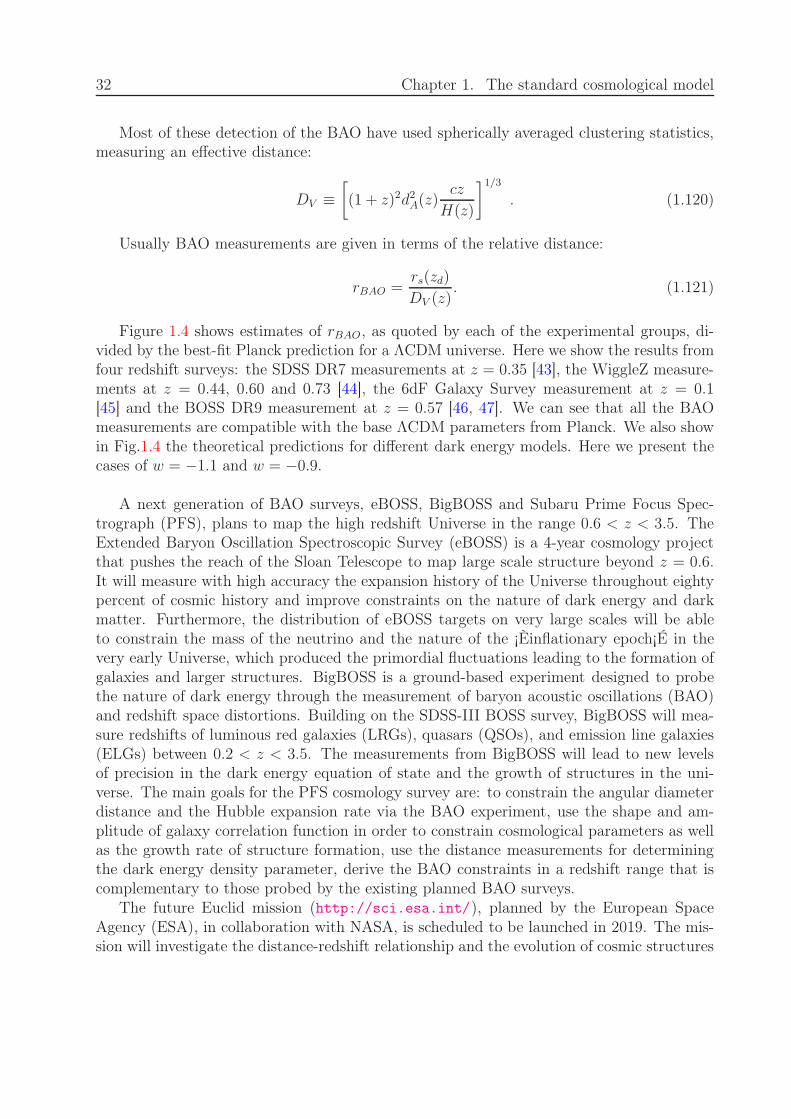
32 Chapter 1. The standard cosmological model
Most of these detection of the BAO have used spherically averaged clustering statistics,measuring an effective distance:
DV ≡[
(1 + z)2d2A(z)
cz
H(z)
]1/3
. (1.120)
Usually BAO measurements are given in terms of the relative distance:
rBAO =rs(zd)
DV (z). (1.121)
Figure 1.4 shows estimates of rBAO, as quoted by each of the experimental groups, di-vided by the best-fit Planck prediction for a ΛCDM universe. Here we show the results fromfour redshift surveys: the SDSS DR7 measurements at z = 0.35 [43], the WiggleZ measure-ments at z = 0.44, 0.60 and 0.73 [44], the 6dF Galaxy Survey measurement at z = 0.1[45] and the BOSS DR9 measurement at z = 0.57 [46, 47]. We can see that all the BAOmeasurements are compatible with the base ΛCDM parameters from Planck. We also showin Fig.1.4 the theoretical predictions for different dark energy models. Here we present thecases of w = −1.1 and w = −0.9.
A next generation of BAO surveys, eBOSS, BigBOSS and Subaru Prime Focus Spec-trograph (PFS), plans to map the high redshift Universe in the range 0.6 < z < 3.5. TheExtended Baryon Oscillation Spectroscopic Survey (eBOSS) is a 4-year cosmology projectthat pushes the reach of the Sloan Telescope to map large scale structure beyond z = 0.6.It will measure with high accuracy the expansion history of the Universe throughout eightypercent of cosmic history and improve constraints on the nature of dark energy and darkmatter. Furthermore, the distribution of eBOSS targets on very large scales will be ableto constrain the mass of the neutrino and the nature of the ¡Èinflationary epoch¡É in thevery early Universe, which produced the primordial fluctuations leading to the formation ofgalaxies and larger structures. BigBOSS is a ground-based experiment designed to probethe nature of dark energy through the measurement of baryon acoustic oscillations (BAO)and redshift space distortions. Building on the SDSS-III BOSS survey, BigBOSS will mea-sure redshifts of luminous red galaxies (LRGs), quasars (QSOs), and emission line galaxies(ELGs) between 0.2 < z < 3.5. The measurements from BigBOSS will lead to new levelsof precision in the dark energy equation of state and the growth of structures in the uni-verse. The main goals for the PFS cosmology survey are: to constrain the angular diameterdistance and the Hubble expansion rate via the BAO experiment, use the shape and am-plitude of galaxy correlation function in order to constrain cosmological parameters as wellas the growth rate of structure formation, use the distance measurements for determiningthe dark energy density parameter, derive the BAO constraints in a redshift range that iscomplementary to those probed by the existing planned BAO surveys.
The future Euclid mission (http://sci.esa.int/), planned by the European SpaceAgency (ESA), in collaboration with NASA, is scheduled to be launched in 2019. The mis-sion will investigate the distance-redshift relationship and the evolution of cosmic structures
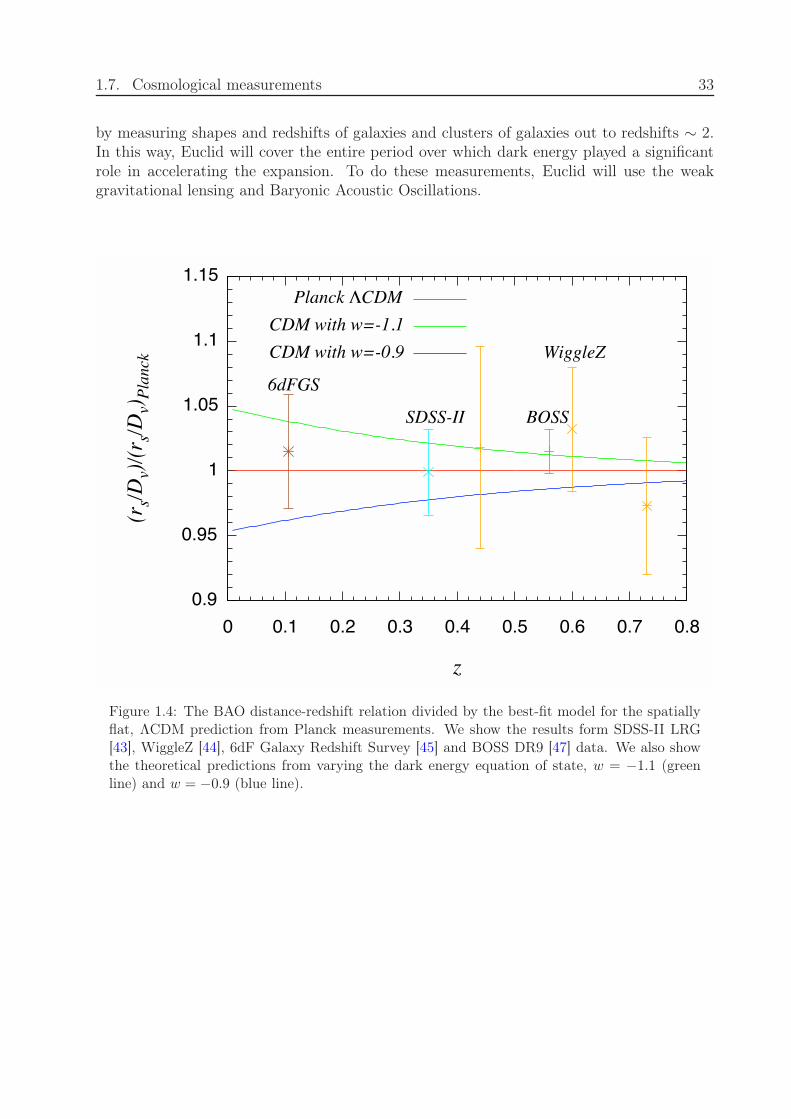
1.7. Cosmological measurements 33
by measuring shapes and redshifts of galaxies and clusters of galaxies out to redshifts ∼ 2.In this way, Euclid will cover the entire period over which dark energy played a significantrole in accelerating the expansion. To do these measurements, Euclid will use the weakgravitational lensing and Baryonic Acoustic Oscillations.
Figure 1.4: The BAO distance-redshift relation divided by the best-fit model for the spatiallyflat, ΛCDM prediction from Planck measurements. We show the results form SDSS-II LRG[43], WiggleZ [44], 6dF Galaxy Redshift Survey [45] and BOSS DR9 [47] data. We also showthe theoretical predictions from varying the dark energy equation of state, w = −1.1 (greenline) and w = −0.9 (blue line).

34 Chapter 1. The standard cosmological model
Chapter 2
Massive neutrinos and Dark Radiation
in Cosmology
In this chapter we introduce neutrinos and their properties. We discuss the neutrino os-cillations and the role of neutrinos in cosmology, describing the impact of massless andmassive neutrinos on cosmological perturbations. We also present some basic properties ofthe Cosmic Neutrino Background, introducing the dark radiation scenario, and we end thechapter illustrating the main effects that neutrinos and dark radiation induce in cosmology,in particular on the CMB and on Large Scale Structure formation.
2.1 Relic neutrinos
The standard hot big bang model predicts the existence of a relic sea of neutrinos thatis in number slightly below to that of relic photons of the CMB. Cosmic neutrinos wereproduced at large temperature in the early universe by frequent weak interactions and theywere maintained in equilibrium with other particles of the primordial plasma. Once thetemperature of the universe reached a few MeV they decoupled from the electromagneticplasma and could travel as free particles, keeping the perfect Fermi-Dirac distribution, eq.(1.84). It is important to note that while a massive Fermi-Dirac distribution is not conservedunder free-streaming, this can be ignored because
∑
mν ≪ 1 MeV.After neutrino decoupling, the photon temperature dropped below the electron mass
favouring e± annihilation, e+e− γγ, that heated the photons. Neutrinos are basically leftundisturbed by pair annihilation, because the analogous weak process e+e− νν have a lowrate compared to the Hubble parameter, and only a tiny fraction of e± goes into neutrinos.Therefore applying entropy conservation and counting interacting degrees of freedom, wecan calculate the ratio of neutrino and photon temperatures (for more details see [17]):
Tν
Tγ=
(
4
11
)1/3
. (2.1)
Given that the CMB temperature is Tγ,0 = 2.725 K, the present relic neutrino tempera-ture is Tν,0 = 1.945 K (1.676 ×10⁻⁴ eV). The number density of relic neutrinos per species
35
36 Chapter 2. Massive neutrinos and Dark Radiation in Cosmology
today is given by:
nν,0 =g
(2π~)3
∫
∞
0
4πp2
e(p)/kBTν0 ± 1dp =
3
11nγ , (2.2)
that leads to a value of 113 neutrinos plus anti-neutrinos of each flavour per cm3. Theenergy density can be calculated numerically, with two analytical limits (relativistic andnon-relativistic):
ρν(mν ≪ Tν) =7π2
120
(
4
11
)4/3
T 4γ , (2.3)
ρν(mν ≫ Tν) = mνnν . (2.4)
Thus, when neutrinos become non-relativistic (at a redshift of ∼ 2000(mν/1eV)), theybehave as matter; while in the relativistic regime they behave as radiation.
Using the present value of the critical density, ρc,0 = 1.054×10⁴h2 eV/cm, and eq. (2.2),we obtain the neutrino density parameter:
Ωνh2 =
∑
imνinν,0
ρc,0=
∑
imνi
93.3 eV, (2.5)
in which we sum only over neutrinos which are non-relativistic today. If they were relativistictoday Ωνh
2 = 6 × 10⁻⁶.Neutrinos fix the expansion rate during the cosmological era when the universe is domi-
nated by radiation. After e± annihilation, the universe was populated only by photons andneutrinos, therefore the corresponding energy density can be written as:
ρr =
[
1 +7
8
(
4
11
)4/3
× 3
]
ργ , (2.6)
in which it is assumed that there are only three light neutrino species and no other rela-tivistic species. However, the three neutrino scenario is a minimal scheme, and there is nofundamental symmetry in nature forcing a definite number of right-handed (sterile) neutrinospecies, as those are allowed in the Standard Model fermion content. For this reason, it isconvenient to parametrize the total radiation energy density in terms of the effective numberof relativistic species Neff :
ρr =
[
1 +7
8
(
4
11
)4/3
Neff
]
ργ . (2.7)
The Standard Model predicts a value of Neff = 3.046, corresponding to the three activeneutrino contribution. The departure of Neff from its standard value, three, is explained inthe following.
In particular, in a more accurate analysis, the assumption of instantaneous neutrinodecoupling can be modified. The main physical reason is that the neutrino plasma receives
2.2. Massive neutrinos 37
a contribution from the e± annihilation and, thus, some relic interactions between e± andneutrinos occur. These processes are more efficient for neutrinos with larger energies thatare more heated, leading to a distortion in the neutrino spectra. A proper calculationof the process of non-instantaneous neutrino decoupling requires the numerical solutionof the Boltzmann equations (see Refs. [48, 49]). Quantum Electrodynamics (QED) finitetemperature corrections and neutrino oscillations need also to be addressed in the Boltzmannequations, see Refs. [50, 51]. The final result, after considering non instantaneous neutrinodecoupling, QED corrections and neutrino oscillations is Neff = 3.046.
Measuring Neff is of great interest today and in this thesis we will consider cosmologicalscenarios where this parameter is not fixed to three, and testing, therefore, sterile neutrinoschemes.
2.2 Massive neutrinos
The existence of neutrino was postulated in 1930 by Wolfgang Pauli, as an attempt to explainthe continuous energy spectrum observed in beta-decay experiments. It was postulated asa neutral particle that scatters only through the weak interaction, and consequently rarelyinteracts with matter. In elementary particle physics, neutrinos are fermions with spin 1/2and they are members of the family of elementary particles called leptons. They differfrom the quarks of the Standard Model (particles with spin 1/2 which participate in strongand electromagnetic interactions) and from the other leptons, which are charged and thusinteract electromagnetically. Due to their very small cross section, the detection of neutrinois particularly challenging. The neutrino was first detected in 1956 in an experiment carriedout by Frederick Reines and Clyde Cowan [52], a quarter of a century after the existence ofthat particle was predicted.
In the Standard Model of elementary particles, neutrinos are massless particles. How-ever, during the last several years, oscillation experiments involving solar, atmospheric, re-actor and accelerator neutrinos have adduced robust evidence for the existence of neutrinooscillations, implying that neutrinos have masses.
2.2.1 Neutrino oscillations
In 1957 Bruno Pontecorvo realized that if neutrinos were massive there could exist processes,named neutrino oscillations, where the neutrino flavour is not conserved. The existence offlavour neutrino oscillations implies that if a neutrino of a given flavour, for example νµ, isproduced in some weak interaction process at a sufficiently large distance from the detectorlocation, the probability to find a neutrino of a different flavour, say ντ , is different fromzero.
Neutrinos are produced and detected, via the weak interaction, as flavour eigenstates νe,νµ or ντ and they propagate as mass eigenstates ν1, ν2 or ν3. In a three-neutrino scenario,the flavour states, α = (e, µ, τ), are related to the mass eigenstates, i=(1, 2, 3), by a mixing
38 Chapter 2. Massive neutrinos and Dark Radiation in Cosmology
matrix called the Pontecorvo-Maki-Nakahawa-Sakata matrix (PMNS) [53, 54]:
|να〉 = Uα,i |νi〉 , (2.8)
which is parametrized as:
Uα,i =
1 0 00 c23 s23
0 −s23 c23
c13 0 s13e−iδ
0 1 0−s13e
iδ 0 c13
c12 s12 0−s12 c12 0
0 0 1
, (2.9)
where cij =cos θij and sij =sin θij for ij = 12, 23 or 13, and δ is a CP-violating phase.We can order the neutrino masses mi such that m3 is the most splitted state and m2 >
m1, and we can define m = m2ij = m2
j − m2i . With this choice, |m2
31| and θ13 arethe atmospheric parameters and m2
21 > 0 and θ12 are the solar parameters. Oscillationexperiments can only measure squared mass differences and the mixing angles, and theircurrent 1σ allowed regions are (see for example [55, 56, 57]):
m221 =
(
7.5+0.18−0.19
)
× 10−5 eV2 , (2.10)
m231 =
(
+2.473+0.070−0.067
)
× 10−3 eV2 , (2.11)
θ12 = 33.36+0.81−0.78 , (2.12)
θ23 = 40.0+2.1−1.5 , (2.13)
θ13 = 8.66+0.44−0.46 . (2.14)
Unfortunately these experiments are not sensitive to the absolute scale of neutrinomasses. Also, current oscillation experiments are unable to extract the sign of |m2
31|,leading to two possible schemes, see Fig. 2.1, known as normal and inverted hierarchies andcharacterized by the sign of m2
31, positive and negative, respectively.
In Fig. 2.2 we show the sum of the three neutrino masses,∑
mν , as a function of themass of the lightest neutrino mass for the normal and inverted hierarchies. The width ofthe curves is related to the current 3σ error on the mass splittings. We can note that in thenormal hierarchy scheme, the minimum value for the sum of neutrino masses is
∑
mν ≃ 0.06eV while in the inverted hierarchy scheme, this value becomes
∑
mν ≃ 0.1 eV.Information on the absolute scale of neutrino masses can be extracted from kinematical
studies of weak decays producing neutrinos. The upper bound on the electron-neutrino massfrom tritium beta decay experiments is m < 2.05−2.3 eV [58, 59]. This bound is expected tobe improved by the KATRIN [60] project to measure neutrino masses in the range 0.3−0.35eV. The neutrinoless double beta decay experiments also put constraints on neutrino masses,providing constraints on the so called effective Majorana mass, mee < 0.36 eV [61]
However the three neutrino oscillation picture is a minimal approach. Additional lightsterile neutrinos (particles that do not interact via any of the fundamental interactions ofthe Standard Model except gravity) may exist in nature, since they are not forbidden by
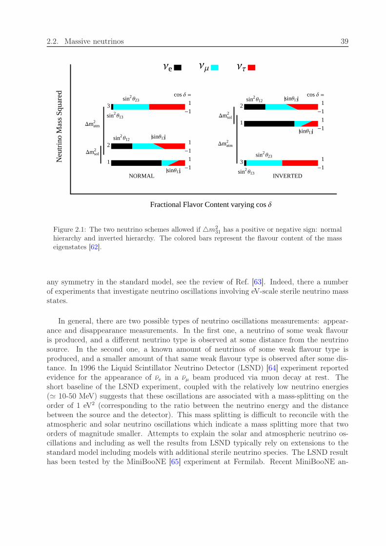
2.2. Massive neutrinos 39
sin2Θ13
1
2
3
sin2Θ12
sin2Θ23
1
-1
1
-1
1
-1
cos ∆ =
NORMAL
Νe ΝΜ ΝΤN
eutr
ino
Mas
sSq
uare
d
Fractional Flavor Content varying cos ∆
Dmsol2
Dmatm2
È ÈsinΘ13
È ÈsinΘ13
sin2Θ13
1
2
3
cos ∆ =
1
-1
1
-1
1
-1
sin2Θ23
sin2Θ12
INVERTED
Dmsol2
Dmatm2
È ÈsinΘ13
È ÈsinΘ13
Figure 2.1: The two neutrino schemes allowed if m231 has a positive or negative sign: normal
hierarchy and inverted hierarchy. The colored bars represent the flavour content of the masseigenstates [62].
any symmetry in the standard model, see the review of Ref. [63]. Indeed, there a numberof experiments that investigate neutrino oscillations involving eV-scale sterile neutrino massstates.
In general, there are two possible types of neutrino oscillations measurements: appear-ance and disappearance measurements. In the first one, a neutrino of some weak flavouris produced, and a different neutrino type is observed at some distance from the neutrinosource. In the second one, a known amount of neutrinos of some weak flavour type isproduced, and a smaller amount of that same weak flavour type is observed after some dis-tance. In 1996 the Liquid Scintillator Neutrino Detector (LSND) [64] experiment reportedevidence for the appearance of νe in a νµ beam produced via muon decay at rest. Theshort baseline of the LSND experiment, coupled with the relatively low neutrino energies(≃ 10-50 MeV) suggests that these oscillations are associated with a mass-splitting on theorder of 1 eV2 (corresponding to the ratio between the neutrino energy and the distancebetween the source and the detector). This mass splitting is difficult to reconcile with theatmospheric and solar neutrino oscillations which indicate a mass splitting more that twoorders of magnitude smaller. Attempts to explain the solar and atmospheric neutrino os-cillations and including as well the results from LSND typically rely on extensions to thestandard model including models with additional sterile neutrino species. The LSND resulthas been tested by the MiniBooNE [65] experiment at Fermilab. Recent MiniBooNE an-
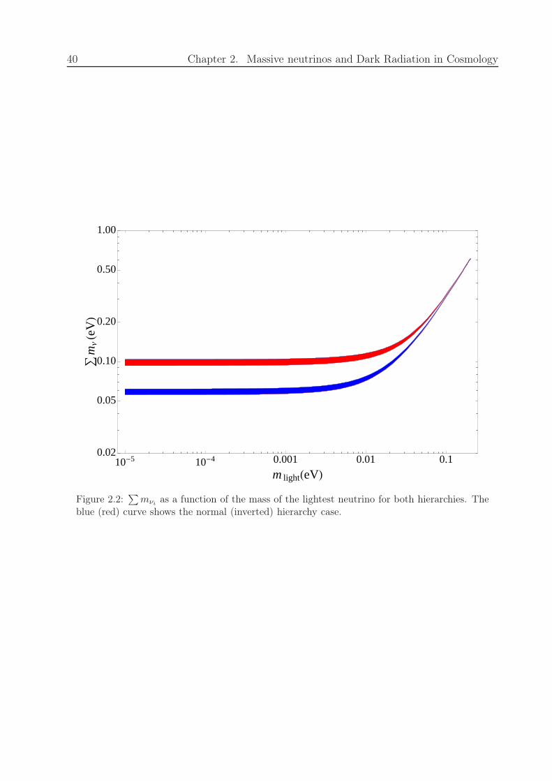
40 Chapter 2. Massive neutrinos and Dark Radiation in Cosmology
10-5 10-4 0.001 0.01 0.10.02
0.05
0.10
0.20
0.50
1.00
m lightHeVL
ÚmΝHe
VL
Figure 2.2:∑
mνias a function of the mass of the lightest neutrino for both hierarchies. The
blue (red) curve shows the normal (inverted) hierarchy case.
2.3. Neutrino cosmological perturbations 41
tineutrino data has some overlap with the evidence for antineutrino oscillations from LSND.The neutrino mode running also shows an excess at low energy, but the energy distributionof the excess is marginally compatible with a simple two neutrino oscillation formalism [66].Models with one additional ∼ 1 eV massive sterile neutrino, i.e. the so called (3+1) models,were introduced to explain LSND short baseline (SBL) antineutrino data [64] by means ofneutrino oscillations. A much better fit to SBL appearance data and, to a lesser extent,to disappearance data, is provided by models with two sterile neutrinos (3+2) [67, 68] orwith three sterile neutrinos (3+3) [69]. While (3+1) and (3+2) models show some tensionwith BBN bounds on N eff
ν , the extra sterile neutrinos do not necessarily have to featurethermal abundances at decoupling, and therefore, these models can be perfectly compatiblewith current cosmological data. In Chapters III and V we will explore the cosmologicalconstraints on massive sterile neutrino scenarios.
2.3 Neutrino cosmological perturbations
Here we present the formalism describing the cosmological perturbations of neutrinos in themassless limit, as well as in the more realistic massive case.
2.3.1 The Boltzmann equation
The evolution of cosmological perturbations associated to relativistic particles, as neutrinos,is governed by the Boltzmann equation, which takes the form:
df
dt= C[f ] , (2.15)
where C denotes the eventual collision terms. In the absence of collisions, the distributionfunction obeys df/dt = 0.
The momentum of each individual neutrino can be labeled by Pi, which is the canonicalconjugate of the comoving coordinate xi. It differs from the proper momentum pi measuredby an observer at a fixed spacial coordinate by:
Pi = a(δij + 12hij)p
j , in synchronous gauge,
Pi = a(1 − φ)pi , in conformal Newtonian gauge. (2.16)
The phase space distribution of the particles gives their number in a differential volumedx1dx2dx3dP1dP2dP3 in phase space:
f(xi, Pj, τ)dx1dx2dx3dP1dP2dP3 = dN . (2.17)
The zero-th order phase space distribution is [8]:
f0 = f0(q) =gs
h3
1
eq/kBT0 ± 1, (2.18)
42 Chapter 2. Massive neutrinos and Dark Radiation in Cosmology
in which + sign refers to the Fermi-Dirac distribution for fermions and − sign is the Bose-Einstein distribution for bosons. The factor gs is the number of spin states and T0 = aTdenotes the temperature of the particles today.
Usually, it is convenient to replace Pj with the comoving 3-momentum, qj = apj , in orderto eliminate the metric perturbation from the definition of the momenta and it is also possibleto express qj in terms of its magnitude and direction: qj = qnj , where nini = δijn
inj = 1.This allows us to replace f(xi, Pj, τ) by f(xi, q, nj, τ) and write the perturbed phase spacedistribution as:
f(xi, q, nj, τ) = f0(q)[1 + Ψ(xi, q, nj, τ)] , (2.19)
where the function Ψ ≪ 1 describe the perturbation to f0.The general expression for the stress-energy tensor computed in terms of the distribution
function and the 4-momentum component is given by:
Tµν =
∫
dP1dP2dP3(−g)−1/2PµPν
P 0f(xi, Pj, τ) , (2.20)
in which g denotes the determinant of gµν . In the synchronous gauge, we have (−g)−1/2 =a−4(1 − 1/2h) and dP1dP2dP3 = (1 − 1/2h)q2dqdΩ up to linear order, where h ≡ hij
and dΩ is the solid angle associated with the direction ni. In the conformal Newtoniangauge, (−g)−1/2 = a−4(1 − ψ + 3φ) and dP1dP2dP3 = (1 − 3φ)q2dqdΩ. Using the relations∫
dΩninj = 4πδij/3 and∫
dΩni =∫
dΩninjnk = 0, from eq. (2.20) it follows that, in bothgauges, the form of energy-momentum tensor is [8]:
T 00 = −a−4
∫
q2dqdΩ√
q2 +m2a2f0(q)(1 + Ψ) , (2.21)
T 0i = a−4
∫
q2dqdΩqnif0(q)Ψ , (2.22)
T ij = a−4
∫
q2dqdΩq2ninj
√
q2 +m2a2f0(q)(1 + Ψ) , (2.23)
to linear order in perturbation theory.We can now write the Boltzmann equation, which describes the evolution of the phase
space distribution, in terms of our variables (xi, q, nj, τ):
df
dt=∂f
∂τ+dxi
dτ
∂f
∂xi+dq
dτ
∂f
∂q+dni
dτ
∂f
∂ni
=
(
∂f
∂τ
)
C
. (2.24)
The terms dni
dτand ∂f
∂niare first-order quantities, thus the term dni
dτ∂f∂ni
in the Boltzmannequation can be neglected to first order. Therefore the Boltzmann equation, in k space andin the two gauges, can be written as [8]:
Synchronous gauge:
dΨ
dτ+ i
q
ǫ(~k · n)Ψ +
d ln f0
d ln q
[
η − h+ 6η
2(k · n)2
]
=1
f0
(
∂f
∂τ
)
C
, (2.25)
2.3. Neutrino cosmological perturbations 43
Newtonian gauge:
dΨ
dτ+ i
q
ǫ(~k · n)Ψ +
d ln f0
d ln q
[
φ− iǫ
q(~k · n)ψ
]
=1
f0
(
∂f
∂τ
)
C
. (2.26)
2.3.2 Massless Neutrinos
The energy density and pressure for massless neutrinos are ρν = 3pν = −T 00 = T i
i . From eq.(2.23), the unperturbed energy density ρν and pressure pν are given by:
ρν = 3pν = a−4
∫
q2dqdΩqf0(q) , (2.27)
and the perturbation in the energy density δρν , in the pressure δpν , in the energy flux δT 0νi
and in the shear stress Σiνj = T i
νj − pνδij are[8] :
δρν = 3δpν = a−4
∫
q2dqdΩqf0(q)Ψ , (2.28)
δT 0νi = a−4
∫
q2dqdΩqnif0(q)Ψ , (2.29)
Σiνj = a−4
∫
q2dqdΩq(ninj −1
3δij)f0(q)Ψ . (2.30)
For a massless neutrino ǫ = q, simplifying the Boltzmann equation. To reduce thenumber of variables we can integrate out the q dependence in the neutrino distributionfunction and expand the angular dependence of the perturbation in a series of Legendrepolynomials Pl(k · n):
Fν(~k, n, τ) ≡∫
q2dqqf0(q)Ψ
q2dqqf0(q)≡
∞∑
l=0
(−i)l(2l + 1)Fν(~k, τ)Pl(k · n) . (2.31)
In terms of Fν(~k, n, τ), the perturbations δν , θν and Σν can be written as:
δν =1
4π
∫
dΩFν(~k, n, τ) = Fν0 , (2.32)
θν =3i
16π
∫
dΩ(~k · n)Fν(~k, n, τ) =3
4kFν1 , (2.33)
Σν = − 3
16π
∫
dΩ
[
(~k · n)2 − 1
3
]
Fν(~k, n, τ) =1
2Fν2 . (2.34)
44 Chapter 2. Massive neutrinos and Dark Radiation in Cosmology
Integrating the equations (2.25) and (2.26) over q2dqqf0(q) and dividing them by∫
q2dqqf0(q),the Boltzmann equations for massless neutrino in the two gauges becomes [8]:
Synchronous gauge
∂Fν
∂τ+ ikµFν = −2
3h− 4
3(h + 6η)P2(µ) , (2.35)
Newtonian gauge∂Fν
∂τ+ ikµFν = 4(φ− ikµψ) , (2.36)
where µ ≡ k · n and Pµ2 = 1/2(3µ2 − 1) is the Legendre polynomial of degree 2. Usingthe Legendre expansion for F , together with the orthonormality property of the Legendrepolynomials and the recursion relation (l+1)Pl+1(µ) = (2l+1)µPl(µ)− lPl−1(µ), we obtain:
Synchronous gauge:
δν = −4
3θν −
2
3h , (2.37a)
θν = k2
(
1
4δν − σν
)
, (2.37b)
Fν2 = 2σν =8
15θν −
3
5kFν3 +
4
5h+
8
5η , (2.37c)
Fνl =k
2l + 1[lFν(l−1) − (l + 1)Fν(l+1)] , l ≥ 3 . (2.37d)
Newtonian gauge:
δν = −4
3θν + 4φ , (2.38a)
θν = k2
(
1
4δν − σν
)
+ k2ψ , (2.38b)
Fνl =k
2l + 1[lFν(l−1) − (l + 1)Fν(l+1)] , l ≥ 3 . (2.38c)
These equations govern the evolution of the phase space distribution of massless neutri-nos. Later in this Chapter we shall see how these equations change in the case of a generaldark radiation fluid.
2.3.3 Massive Neutrinos
Massive neutrinos also obey the collisionless Bolztmann equations. However, their distribu-tion function is complicated by the fact that they have a non zero mass. From eq. (2.23),

2.3. Neutrino cosmological perturbations 45
the unperturbed energy density and pressure for massive neutrinos are given by [8]:
ρν = a−4
∫
q2dqdΩǫf0(q) , (2.39)
pν =1
3a−4
∫
q2dqdΩq2
ǫf0(q) , (2.40)
where ǫ =√
q2 +m2νa
2.The perturbations are:
δρν = a−4
∫
q2dqdΩǫf0(q)Ψ , (2.41)
δpν =1
3a−4
∫
q2dqdΩq2
ǫf0(q)Ψ , (2.42)
δT 0νi = a−4
∫
q2dqdΩqnif0(q)Ψ , (2.43)
Σiνj = a−4
∫
q2dqdΩq2
ǫ(ninj −
1
3δij)f0(q)Ψ . (2.44)
In this case we cannot integrate out the q dependence in the distribution function, aswe did for the massless neutrinos, because ǫ(q, τ) depends on the momentum and time.However, it is possible to expand the perturbation Ψ in multipoles space:
Ψ(~k, n, q, τ)=∞∑
l=0
(−i)l(2l + 1)Ψl((~k, q, τ)Pl(k · n) . (2.45)
Therefore the perturbed energy density, pressure, energy flux and shear stress in k-spacebecome:
δρν = 4πa−4
∫
q2dqǫf0(q)Ψ0 , (2.46)
δpν =4π
3a−4
∫
q2dqq2
ǫf0(q)Ψ0 , (2.47)
(ρν + pν)θν = 4πka−4
∫
q2dqqf0(q)Ψ1 , (2.48)
(ρν + pν)σν =8π
3a−4
∫
q2dqq2
ǫf0(q)Ψ2 . (2.49)
Following the same strategy used for massless neutrinos, we can obtain the Boltzmannequations for massive neutrinos in the two gauges:

46 Chapter 2. Massive neutrinos and Dark Radiation in Cosmology
Synchronous gauge:
Ψ0 = −qkǫ
Ψ1 −1
6hd ln f0
d ln q, (2.50a)
Ψ1 =qk
3ǫ(Ψ0 − 2Ψ2) , (2.50b)
Ψ2 =qk
5ǫ(2Ψ1 − 3Ψ3) −
(
1
15h+
2
5η
)
d ln f0
d ln q, (2.50c)
Ψl =qk
(2l + 1)ǫ[lΨ(l−1) − (l + 1)Ψ(l+1)] , l ≥ 3 . (2.50d)
Newtonian gauge:
Ψ0 = −qkǫ
Ψ1 − φd ln f0
d ln q, (2.51a)
Ψ1 =qk
3ǫ(Ψ0 − 2Ψ2) − ǫk
3qΨd ln f0
d ln q, (2.51b)
Ψl =qk
(2l + 1)ǫ[lΨ(l−1) − (l + 1)Ψ(l+1)] , l ≥ 2 . (2.51c)
Because of the q dependence, the integration of these equations is computationally ex-pensive.
2.4 Dark radiation models
One of the major theoretical predictions of standard cosmology is the existence of a relativis-itc energy component (Cosmic Neutrino Background, CNB), besides CMB photons, whoseenergy density is given by eq. (2.7). The cosmological abundance of relativistic particlesas active or steriles neutrinos or any other light particle is parametrized in terms of theeffective number of relativistic degrees of freedom Neff . As we have seen in section 2.1, theexpected value of Neff is 3.046, which corresponds to the standard case of the three activeneutrino species.
In recent years, cosmological data seem to suggest values forNeff higher than the standardone. Measurements of CMB anisotropies from WMAP combined with ACT, SPT, BAO andHST data sets have provided the constraint Neff = 3.84 ± 0.40 [18]; more recently, Planckdata combined with WMAP polarization, high-ℓ CMB data and BAO have reported thebound Neff = 3.30+0.54
−0.51 at 95% CL [9].A larger value for Neff could arise from new physics, not only related to sterile neutrinos,
as is the case of axions [70, 71], decaying of non-relativistic matter models [72], gravity waves[73], extra dimension [74, 75, 76], dark energy [77] or asymmetric dark matter models [78].Information on the dark relativistic background can be obtained not only from its effectson the expansion rate of the universe but also from its clustering properties. For example,
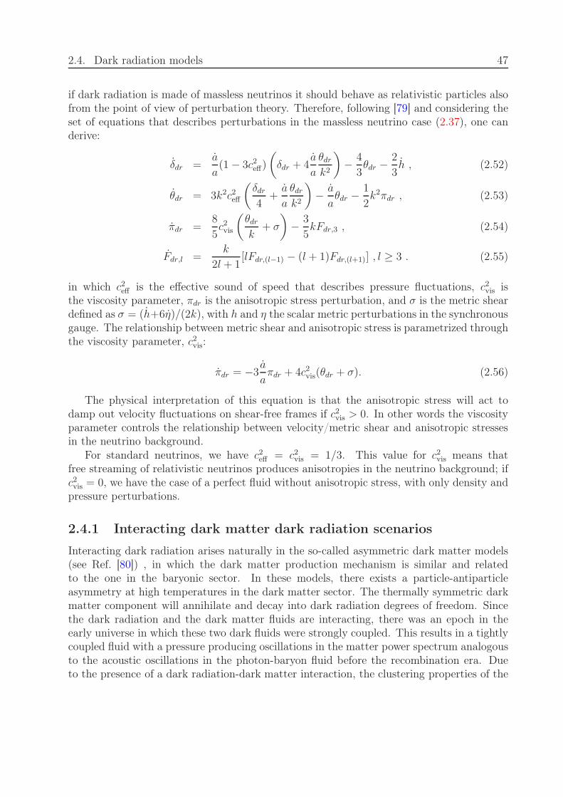
2.4. Dark radiation models 47
if dark radiation is made of massless neutrinos it should behave as relativistic particles alsofrom the point of view of perturbation theory. Therefore, following [79] and considering theset of equations that describes perturbations in the massless neutrino case (2.37), one canderive:
δdr =a
a(1 − 3c2eff)
(
δdr + 4a
a
θdr
k2
)
− 4
3θdr −
2
3h , (2.52)
θdr = 3k2c2eff
(
δdr
4+a
a
θdr
k2
)
− a
aθdr −
1
2k2πdr , (2.53)
πdr =8
5c2vis
(
θdr
k+ σ
)
− 3
5kFdr,3 , (2.54)
Fdr,l =k
2l + 1[lFdr,(l−1) − (l + 1)Fdr,(l+1)] , l ≥ 3 . (2.55)
in which c2eff is the effective sound of speed that describes pressure fluctuations, c2vis isthe viscosity parameter, πdr is the anisotropic stress perturbation, and σ is the metric sheardefined as σ = (h+6η)/(2k), with h and η the scalar metric perturbations in the synchronousgauge. The relationship between metric shear and anisotropic stress is parametrized throughthe viscosity parameter, c2vis:
πdr = −3a
aπdr + 4c2vis(θdr + σ). (2.56)
The physical interpretation of this equation is that the anisotropic stress will act todamp out velocity fluctuations on shear-free frames if c2vis > 0. In other words the viscosityparameter controls the relationship between velocity/metric shear and anisotropic stressesin the neutrino background.
For standard neutrinos, we have c2eff = c2vis = 1/3. This value for c2vis means thatfree streaming of relativistic neutrinos produces anisotropies in the neutrino background; ifc2vis = 0, we have the case of a perfect fluid without anisotropic stress, with only density andpressure perturbations.
2.4.1 Interacting dark matter dark radiation scenarios
Interacting dark radiation arises naturally in the so-called asymmetric dark matter models(see Ref. [80]) , in which the dark matter production mechanism is similar and relatedto the one in the baryonic sector. In these models, there exists a particle-antiparticleasymmetry at high temperatures in the dark matter sector. The thermally symmetric darkmatter component will annihilate and decay into dark radiation degrees of freedom. Sincethe dark radiation and the dark matter fluids are interacting, there was an epoch in theearly universe in which these two dark fluids were strongly coupled. This results in a tightlycoupled fluid with a pressure producing oscillations in the matter power spectrum analogousto the acoustic oscillations in the photon-baryon fluid before the recombination era. Dueto the presence of a dark radiation-dark matter interaction, the clustering properties of the

48 Chapter 2. Massive neutrinos and Dark Radiation in Cosmology
dark radiation component can be modified. In other words, if dark radiation is made ofinteracting particles, the values of the clustering parameters c2eff and c2vis may differ from thecanonical c2eff = c2vis = 1/3.
The dark matter component behaves as a non-relativistic fluid described, in the uncou-pled case, by the equations (1.53) with δp/δρ = w = 0 and metric shear σ = 0. The darkradiation component is described by the equations (2.52) and (2.53). In the presence of adark radiation-dark matter interaction, the modified Euler equations for these two fluidsread:
θdm = − aaθdm +
4ρdr
3ρdm
andmσdm−dr(θdr − θdm) , (2.57)
θdr =1
4k2(δdr − 2πdr) + andmσdm−dr(θdm − θdr) , (2.58)
in which we have considered the standard value of c2eff for brevity. The term andmσdm−dr(θdm−θdr) in eq. (2.58) represents the momentum transferred to the dark radiation componentand the quantity andmσdm−dr is the differential opacity which gives the scattering rate ofdark radiation by dark matter.
The complete Euler equation for dark radiation, including the interaction term with darkmatter, reads:
θdr = 3k2c2eff
(
1
4δdr −
a
a
θdr
k2
)
− a
aθdr −
1
2k2πdr + andmσdm−dr(θdm − θdr) . (2.59)
It is convenient [81] to parametrize the coupling between dark radiation and dark matterthrough a cross section given by:
〈σdm−dr|v|〉 ∼ Q0 mdm , (2.60)
if it is constant, or
〈σdm−dr|v|〉 ∼Q2
a2mdm , (2.61)
if it is proportional to T 2, where the parameters Q0 and Q2 are constants in cm2 MeV−1
units. It has been shown in Ref. [78] that the cosmological implications of both constantand T-dependent interacting cross sections are very similar. In Chapter VI we will presentthe cosmological constraints on interacting dark radiation schemes assuming a constant in-teraction rate.
In the next section we will explain the impact of dark radiation species on the CMB andon Large Scale Structure measurements.
2.5 Neutrino properties and cosmological observations
2.5.1 Standard cosmology plus three massive neutrinos
Cosmology can provide strong bounds for the sum of the neutrino masses. This is becauseneutrinos play a relevant role in large-scale structure formation and leave key signatures in

2.5. Neutrino properties and cosmological observations 49
several cosmological data sets.If a fraction of the dark matter is made up of neutrinos (Ωm = Ωb + ΩDM = Ωb +
ΩCDM + Ων), they modify the evolution of matter perturbations. In particular, once theCDM perturbations enter into the matter dominated era, neutrinos will slow down therate at which these perturbations grow. In order to understand this effect, we use eq.(1.63) to compute the linear growth of CDM perturbations in a universe containing massiveneutrinos. The difference with the equation governing the evolution of CDM perturbationsin a neutrinoless universe is that neutrinos affect the expansion rate:
H2 =8πG
3(ρCDM + ρν + ρb) . (2.62)
Let us assume that neutrinos are non-relativistic at some epoch of the matter dominatedera and we introduce the parameter:
fν =ρν
(ρCDM + ρb + ρν)=
Ων
Ωm
, (2.63)
whose value remains approximately constant because the neutrino energy density will scaleas ρν ∝ a−3. Then, the scale factor still evolves like τ 2 and the equation of evolution readsas1:
δCDM +2
τδCDM − 6
τ 2(1 − fν)δCDM = 0 , (2.64)
whose solutions are δCDM = Aτα+ +Bτα− , with:
α± =−1 ±
√
1 + 24(1 − fν)
4. (2.65)
Therefore, in the matter dominated era, the growth of CDM perturbations is suppressedby the presence of massive neutrinos as:
D1(a) ≃ a1−(3/5)fν . (2.66)
The growth of CDM perturbations is reduced due the fact that one of the componentin the universe contributes to the homogeneous expansion rate but not to the gravitationalclustering.
In Fig. 2.3 we plot the linear power spectrum, computed with CAMB [82], for a mass-less neutrino universe using the best fit parameters from Planck measurements, [9], (redline). We also plot the linear power spectrum of different cosmological models with threedegenerate massive neutrinos.
Notice that neutrinos suppress the power on spatial scales below the free streaming scalewhen they become non relativistic (we will carefully explain this effect in Chapter IV). Theredshift at which neutrinos become non relativistic reads
1 + znr ≃ 1890( mν
1 eV
)
, (2.67)
1This equation refers to spatial scales smaller than the neutrino free streaming scale.

50 Chapter 2. Massive neutrinos and Dark Radiation in Cosmology
Figure 2.3: Linear power spectrum for three cosmological models with three degenerate massiveneutrinos and for one with massless neutrinos. The red line depicts the matter power spectrumP (k) for the best fit parameters for a ΛCDM model with massless neutrinos from the Planckdata set. Neutrino free-streaming produces a decrease in the amplitude of the power spectrumon small scales.
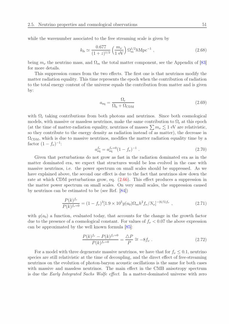
2.5. Neutrino properties and cosmological observations 51
while the wavenumber associated to the free streaming scale is given by
kfs ≃0.677
(1 + z)1/2
( mν
1 eV
)
Ω1/2m hMpc−1 , (2.68)
being mν the neutrino mass, and Ωm the total matter component, see the Appendix of [83]for more details.
This suppression comes from the two effects. The first one is that neutrinos modify thematter radiation equality. This time represents the epoch when the contribution of radiationto the total energy content of the universe equals the contribution from matter and is givenby:
aeq =Ωr
Ωb + ΩCDM(2.69)
with Ωr taking contributions from both photons and neutrinos. Since both cosmologicalmodels, with massive or massless neutrinos, make the same contribution to Ωr at this epoch(at the time of matter-radiation equality, neutrinos of masses
∑
mν . 1 eV are relativistic,so they contribute to the energy density as radiation instead of as matter), the decrease inΩCDM, which is due to massive neutrinos, modifies the matter radiation equality time by afactor (1 − fν)
−1:afν
eq = afν=0eq (1 − fν)
−1 . (2.70)
Given that perturbations do not grow as fast in the radiation dominated era as in thematter dominated era, we expect that structures would be less evolved in the case withmassive neutrinos, i.e. the power spectrum on small scales should be suppressed. As wehave explained above, the second one effect is due to the fact that neutrinos slow down therate at which CDM perturbations grow, eq. (2.66). This effect produces a suppression inthe matter power spectrum on small scales. On very small scales, the suppression causedby neutrinos can be estimated to be (see Ref. [84])
P (k)fν
P (k)fν=0= (1 − fν)
3[1.9 × 10⁵g(a0)Ωmh2fν/Nν]
−(6/5)fν , (2.71)
with g(a0) a function, evaluated today, that accounts for the change in the growth factordue to the presence of a cosmological constant. For values of fν < 0.07 the above expressioncan be approximated by the well known formula [85]:
P (k)fν − P (k)fν=0
P (k)fν=0=
PP
∼= −8fν . (2.72)
For a model with three degenerate massive neutrinos, we have that for fν ≤ 0.1, neutrinospecies are still relativistic at the time of decoupling, and the direct effect of free-streamingneutrinos on the evolution of photon-baryon acoustic oscillations is the same for both caseswith massive and massless neutrinos. The main effect in the CMB anisotropy spectrumis due the Early Integrated Sachs Wolfe effect. In a matter-dominated universe with zero
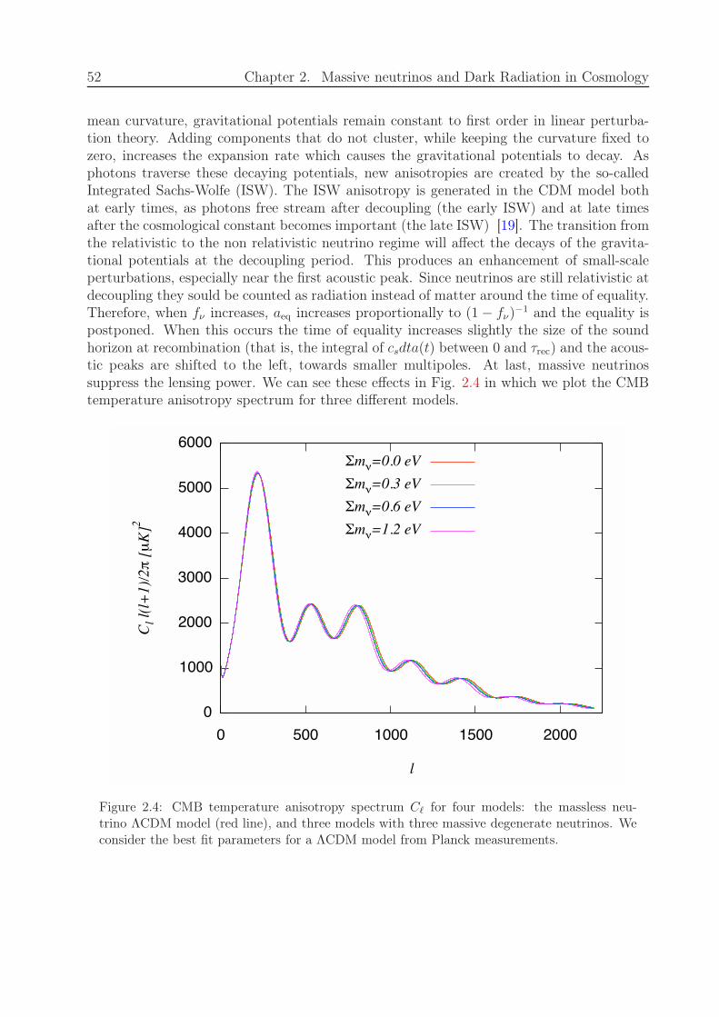
52 Chapter 2. Massive neutrinos and Dark Radiation in Cosmology
mean curvature, gravitational potentials remain constant to first order in linear perturba-tion theory. Adding components that do not cluster, while keeping the curvature fixed tozero, increases the expansion rate which causes the gravitational potentials to decay. Asphotons traverse these decaying potentials, new anisotropies are created by the so-calledIntegrated Sachs-Wolfe (ISW). The ISW anisotropy is generated in the CDM model bothat early times, as photons free stream after decoupling (the early ISW) and at late timesafter the cosmological constant becomes important (the late ISW) [19]. The transition fromthe relativistic to the non relativistic neutrino regime will affect the decays of the gravita-tional potentials at the decoupling period. This produces an enhancement of small-scaleperturbations, especially near the first acoustic peak. Since neutrinos are still relativistic atdecoupling they sould be counted as radiation instead of matter around the time of equality.Therefore, when fν increases, aeq increases proportionally to (1 − fν)
−1 and the equality ispostponed. When this occurs the time of equality increases slightly the size of the soundhorizon at recombination (that is, the integral of csdta(t) between 0 and τrec) and the acous-tic peaks are shifted to the left, towards smaller multipoles. At last, massive neutrinossuppress the lensing power. We can see these effects in Fig. 2.4 in which we plot the CMBtemperature anisotropy spectrum for three different models.
Figure 2.4: CMB temperature anisotropy spectrum Cℓ for four models: the massless neu-trino ΛCDM model (red line), and three models with three massive degenerate neutrinos. Weconsider the best fit parameters for a ΛCDM model from Planck measurements.
2.5. Neutrino properties and cosmological observations 53
If neutrinos were heavier than a few eV, they would be already non-relativistic at de-coupling. This case would require a more complicated description that would affect thephoton-baryon fluid. However, we will see in this thesis that this situation is highly dis-favoured by current cosmological data.
Since the two-dimensional (2D) power spectrum of galaxies is related to 3D matter powerspectrum P (k), eq. (1.105), in the presence of massive neutrinos, also the angular powerspectrum is suppressed at any redshift and this suppression could be partially compensatedby increasing the cold dark matter energy density. In Fig. 2.5 we illustrate this effect forfour models with different values of
∑
mν .
Figure 2.5: Effect of neutrinos on the matter angular power spectra, Cℓ, for the best fitparameters for a ΛCDM model from the Planck data. We consider four cases with differentvalues of
∑
mν . The data correspond to the observed power spectrum obtained from BOSSDR8 in the redshift bin 0.45< z <0.5 [40]. The red line depicts 2D spectra for a ΛCDM modelassuming no massive neutrino species.
The impact of massive neutrinos on the Cℓ power spectra will be carefully analysed inSec. IV.
Measurements of all of these observables have been used to place new bounds on neutrinophysics from cosmology, setting an upper limit on the neutrino mass below ∼ 0.5 eV. Recent
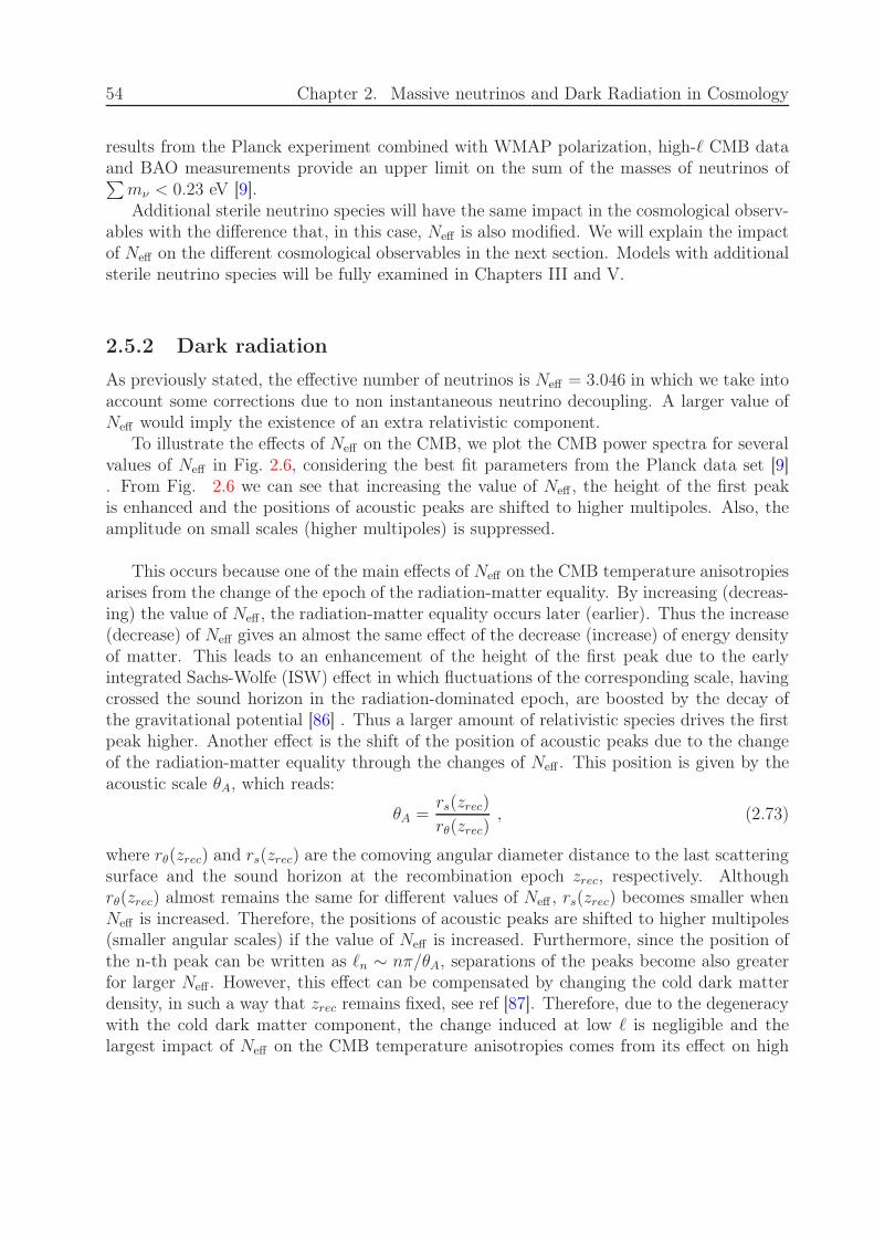
54 Chapter 2. Massive neutrinos and Dark Radiation in Cosmology
results from the Planck experiment combined with WMAP polarization, high-ℓ CMB dataand BAO measurements provide an upper limit on the sum of the masses of neutrinos of∑
mν < 0.23 eV [9].Additional sterile neutrino species will have the same impact in the cosmological observ-
ables with the difference that, in this case, Neff is also modified. We will explain the impactof Neff on the different cosmological observables in the next section. Models with additionalsterile neutrino species will be fully examined in Chapters III and V.
2.5.2 Dark radiation
As previously stated, the effective number of neutrinos is Neff = 3.046 in which we take intoaccount some corrections due to non instantaneous neutrino decoupling. A larger value ofNeff would imply the existence of an extra relativistic component.
To illustrate the effects of Neff on the CMB, we plot the CMB power spectra for severalvalues of Neff in Fig. 2.6, considering the best fit parameters from the Planck data set [9]. From Fig. 2.6 we can see that increasing the value of Neff , the height of the first peakis enhanced and the positions of acoustic peaks are shifted to higher multipoles. Also, theamplitude on small scales (higher multipoles) is suppressed.
This occurs because one of the main effects of Neff on the CMB temperature anisotropiesarises from the change of the epoch of the radiation-matter equality. By increasing (decreas-ing) the value of Neff , the radiation-matter equality occurs later (earlier). Thus the increase(decrease) of Neff gives an almost the same effect of the decrease (increase) of energy densityof matter. This leads to an enhancement of the height of the first peak due to the earlyintegrated Sachs-Wolfe (ISW) effect in which fluctuations of the corresponding scale, havingcrossed the sound horizon in the radiation-dominated epoch, are boosted by the decay ofthe gravitational potential [86] . Thus a larger amount of relativistic species drives the firstpeak higher. Another effect is the shift of the position of acoustic peaks due to the changeof the radiation-matter equality through the changes of Neff . This position is given by theacoustic scale θA, which reads:
θA =rs(zrec)
rθ(zrec), (2.73)
where rθ(zrec) and rs(zrec) are the comoving angular diameter distance to the last scatteringsurface and the sound horizon at the recombination epoch zrec, respectively. Althoughrθ(zrec) almost remains the same for different values of Neff , rs(zrec) becomes smaller whenNeff is increased. Therefore, the positions of acoustic peaks are shifted to higher multipoles(smaller angular scales) if the value of Neff is increased. Furthermore, since the position ofthe n-th peak can be written as ℓn ∼ nπ/θA, separations of the peaks become also greaterfor larger Neff . However, this effect can be compensated by changing the cold dark matterdensity, in such a way that zrec remains fixed, see ref [87]. Therefore, due to the degeneracywith the cold dark matter component, the change induced at low ℓ is negligible and thelargest impact of Neff on the CMB temperature anisotropies comes from its effect on high
2.5. Neutrino properties and cosmological observations 55
Figure 2.6: CMB temperature power spectrum Cℓ for five models with a different value of Neff
considering the best fit parameters for a ΛCDM model from the Planck data. The red linedepicts the standard case with Neff = 3.046. An increase of Neff leads to an enhancement ofthe first peak and a shift of the acoustic peaks towards higher multipoles.
multipoles ℓ, since a higher value of Neff will induce a drop in power at small scales due toan increased Silk damping. Silk damping refers to the suppression in power of the CMBtemperature anisotropies on scales smaller than the photon diffusion length.
An increase of the effective number of neutrino Neff also produces a suppression in thematter power spectrum due to the change in the epoch of matter-radiation equality.
A change in the effective sound speed c2eff and in the viscosity parameter c2vis affects boththe CMB spectrum and the matter power spectrum.
Varying c2vis modifies the ability of the dark radiation to free-stream out of the potentialwells. In particular, lowering c2vis to the value c2vis = 0, the TT power spectrum is enhancedwith respect to the standard case. This situation can be explained, roughly, as the darkradiation component becoming a perfect fluid. That is, we are dealing with a single fluidcharacterized by an effective viscosity. Disregarding the fluid nature and the physical originof the viscosity, the general consideration holds: for a given perturbation induced in thefluid, the amplitude of the oscillations that the viscosity produces increases as the viscosity
56 Chapter 2. Massive neutrinos and Dark Radiation in Cosmology
is reduced. Therefore, lowering c2vis diminishes the amount of damping induced by the darkradiation viscosity, and, consequently, the amplitude of the CMB oscillations will increase,increasing in turn the amplitude of the angular power spectrum.
On the other hand, a change of c2eff implies a decrease of pressure perturbations forthe dark radiation components in its rest frame. In particular, a decrease in c2eff from itscanonical 1/3 to the value c2eff = 0 leads to a damping of the CMB peaks, since dark radiationis behaving as a pressureless fluid from the perturbation perspective. Thus as c2eff decreases,the height of the acoustic peaks decreases.
While varying the viscosity parameter c2vis, the matter power barely change, a changein c2eff changes dramatically. For instance, if c2eff = 0, dark radiation is a pressureless fluidwhich behaves as dark matter, inducing an enhancement of the matter fluctuations.
These perturbation parameters can be constrained through measurements of the CMBanisotropies since dark radiation is coupled through gravity with all the remaining com-ponents. This opens a new window for testing the dark radiation component, since, forexample, a smaller value for c2vis could indicate possible non standard interactions. Con-straints on these parameters have been obtained by several authors, since the observation ofdeviations from the standard values could hint for non-standard physics. The most recentconstraints for c2eff and c2vis have been obtained combining current Planck data with WMAPlow-ℓ measurements for polarization plus BAO and HST data sets: c2eff = 0.306± 0.013 andc2vis = 0.53 ± 0.16 [88].
In Chapter V, we will present bounds from recent cosmological data on the dark radia-tion parameters Neff , c2eff and c2vis extending the ΛCDM cosmological model and analyzingthe correlations among the dark radiation parameters and the remaining cosmological pa-rameters, as the dark energy equation of state or the scalar spectral index. In Chapter VI,we will explore the bounds on Neff ,c2eff and c2vis considering a ΛCDM cosmology plus a darkradiation-dark matter interaction.
Part II
Scientific Research
57

Chapter 3
Constraints on massive sterile neutrino
species from current and future
cosmological data
In this Chapter we study a flat ΛCDM scenario with Neff active plus sterile massive neutrinospecies, in order to test the so-called (3+2) model with cosmological data. This Chapter isa copy of the paper:
Constraints on massive sterile neutrino species from current and future cosmologicaldata, Elena Giusarma, Martina Corsi, Maria Archidiacono, Roland De Putter, AlessandroMelchiorri, Olga Mena & Stefania Pandolfi, 2011, Physical Review D83, 115023.
3.1 Introduction
Solar, atmospheric, reactor, and accelerator neutrinos have provided compelling evidencefor the existence of neutrino oscillations, implying non-zero neutrino masses (see Ref. [89]and references therein). The present data require the number of massive neutrinos to beequal or larger than two, since there are at least two mass squared differences (∆m2
atmos and∆m2
solar) driving the atmospheric and solar neutrino oscillations respectively. Unfortunately,oscillation experiments only provide bounds on the neutrino mass squared differences, i.e.they are not sensitive to the overall neutrino mass scale.
Cosmology provides one of the means to tackle the absolute scale of neutrino masses.Neutrinos can leave key signatures in several cosmological data sets. The amount of primor-dial relativistic neutrinos changes the epoch of the matter- radiation equality, leaving animprint on both Cosmic Microwave Background (CMB) anisotropies (through the so-calledIntegrated Sachs-Wolfe effect) and on structure formation, while non relativistic neutrinosin the recent Universe suppress the growth of matter density fluctuations and galaxy clus-tering, see Ref. [84]. Cosmology can therefore weigh neutrinos, providing an upper boundon the sum of the three active neutrino masses,
∑
mν ∼ 0.58 eV at the 95% CL [90]. Theformer bound is found when CMB measurements from the Wilkinson Microwave Anisotropy
59

60Chapter 3. Constraints on massive sterile neutrino species from current and future
cosmological data
Probe (WMAP) are combined with measurements of the distribution of galaxies (SDSSII-BAO) and of the Hubble constant H0 (HST) 1 in the assumption of a flat universe with acosmological constant, i.e. a ΛCDM cosmology.
However, the three neutrino scenario is a minimal scheme, and there is no fundamentalsymmetry in nature forcing a definite number of right-handed (sterile) neutrino species,as those are allowed in the Standard Model fermion content. Indeed, cosmological probeshave been extensively used to set bounds on the relativistic energy density of the universein terms of the effective number of neutrinos N eff
ν (see, for instance, Refs. [91, 92, 93,94, 95]). Currently, WMAP, SDSSII-BAO and HST data provide a 68% CL range onN eff
ν = 4.34+0.86−0.88 [90] in the assumption of a ΛCDM universe. If the effective number of
neutrinos N effν is larger than the Standard Model prediction of N eff
ν = 3.046 at the BigBang Nucleosynthesis (BBN) era, the relativistic degrees of freedom, and, consequently, theHubble expansion rate will also be larger causing weak interactions to become uneffectiveearlier. This will lead to a larger neutron-to-proton ratio and will change the standard BBNpredictions for light element abundances. Combining Deuterium and 4He data, the authorsof Ref. [93] found N eff
ν = 3.1+1.4−1.2 at the 95% CL.
Models with one additional ∼ 1 eV massive sterile neutrino, i.e. the so called (3+1)models, were introduced to explain LSND short baseline (SBL) antineutrino data [64] bymeans of neutrino oscillations. A much better fit to SBL appearance data and, to a lesserextent, to disappearance data, is provided by models with two sterile neutrinos (3+2) [67, 68]which can also explain both the MiniBooNE neutrino [65] and antineutrino data [96] if CPviolation is allowed [97]. CP violation can even occur in (3+1) scenarios with only onerelevant mass squared difference in the presence of non standard neutrino interactions (NSI).Therefore, the (3+1) NSI model can also nicely explain current data [98]. While (3+1) and(3+2) models show some tension with BBN bounds on N eff
ν , the extra sterile neutrinos donot necessarily have to feature thermal abundances at decoupling. The first analysis ofboth SBL oscillation data and cosmological data was performed by the authors of Ref. [99],where the usual full thermalization scenario for the sterile neutrino species was not assumed.Instead, the sterile abundances were computed taking into account the multi flavour mixingprocesses operating at the neutrino decoupling period. Robust bounds on sterile neutrinomasses, mixings and abundances were derived. However, the masses of the three activeneutrinos were fixed to m1 ∼ 0, m2 ∼
√
∆m2solar and m3 ∼
√
∆m2atmos. In Ref. [100] the
authors derived the bounds on a light sterile neutrino scenario enlarging the usual thermalscenario. More recently, the authors of Ref. [101] have used current cosmological data toanalyze two possible active plus sterile neutrino scenarios, one with massless active neutrinos(and massive steriles) and the other one with massless steriles states of unknown number(and massive active species). However, there are no cosmological bounds on the more naturaland oscillation-data motivated scenario in which both the sterile and the active neutrinoshave masses. Active neutrinos are massive; this is what oscillation data are telling us. In thesame way, the LSND and MiniBooNE antineutrino data, if explained in terms of neutrinooscillations, point to the existence of massive sterile neutrino species. What oscillation data
1For other recent analyses, see also Refs. [91, 92].
3.2. Current constraints 61
can not tell us is the absolute scale of neutrino masses and this is precisely what we addressin this study, in the spirit of Ref. [102], via present and future cosmological measurements.
The paper is organized as follows. In Sec. 3.2 we present the constraints on the activeand sterile neutrino masses and on the number of sterile species from current cosmologicaldata as well as from BBN measurements of light element abundances. Section 3.3 is devotedto future errors on these parameters. We describe the Fisher matrix method used here forforecasting errors and discuss the potential results from the ongoing Planck CMB missioncombined with future BOSS and Euclid galaxy survey data. We also describe the inducedbiases on some parameters (such as H0 and mν) when the cosmological model does notaccount for the presence of sterile states to describe the data. We conclude in Sec. 3.4.
3.2 Current constraints
Here we summarize the constraints from current data on the active neutrino masses andon the sterile neutrino thermal abundance and masses. We have modified the BoltzmannCAMB code [82] incorporating the extra massive sterile neutrino parameters and extractedcosmological parameters from current data using a Monte Carlo Markov Chain (MCMC)analysis based on the publicly available MCMC package cosmomc[103]. We consider here aflat ΛCDM scenario plus three (Nνs) active (sterile) massive neutrino species, described bya set of cosmological parameters
ωb, ωc,Θs, τ, ns, log[1010As], mν , mνs , Nνs , (3.1)
where ωb ≡ Ωbh2 and ωc ≡ Ωch
2 are the physical baryon and cold dark matter densities, Θs
is the ratio between the sound horizon and the angular diameter distance at decoupling, τis the optical depth, ns is the scalar spectral index, As is the amplitude of the primordialspectrum 2, mν is the active neutrino mass, mνs is the sterile neutrino mass and Nνs isthe number of thermalized sterile neutrino species. We assume that both active and sterileneutrinos have degenerate mass spectra (mν and mνs are the individual masses, not thesum of the masses). The flat priors assumed on these cosmological parameters are shownin Tab. 6.1.
Our basic data set is the seven–year WMAP data [90, 104] (temperature and polar-ization) with the routine for computing the likelihood supplied by the WMAP team. Weconsider two cases: we first analyze the WMAP data together with the luminous red galaxyclustering results from SDSSII (Sloan Digital Sky Survey) [105] and with a prior on theHubble constant from HST (Hubble Space Telescope) [106], referring to it as the “run1”case. We then include to these data sets Supernova Ia Union Compilation 2 data [15],and we will refer to this case as “run2”. In addition, we also add to the previous datasets the BBN measurements of the 4He abundance, considering separately helium fractionsof Y 1
p = 0.2561 ± 0.0108 (see Ref. [107]) and of Y 2p = 0.2565 ± 0.0010 (stat.) ±0.0050
(syst.) from Ref. [108]. Finally, we also consider the Deuterium abundance measurementslog(D/H) = 4.56 ± 0.04 from Ref. [109].
2The pivot scale assumed in this study corresponds to k0 = 0.05 Mpc−1.

62Chapter 3. Constraints on massive sterile neutrino species from current and future
cosmological data
Parameter PriorΩbh
2 0.005-0.1Ωch
2 0.01-0.99Θs 0.5-10τ 0.01-0.8ns 0.5-1.5
ln (1010As) 2.7-4mνs [eV] 0-3mν [eV] 0-3Nνs 0-6
Table 3.1: Flat priors for the cosmological parameters considered here.
It is important to clarify that CMB anisotropies also depend on the value of Yp butsince Yp is constrained loosely by current CMB/LSS data, it is consistent to fix it to valueYp = 0.24 in the CMB runs and to consider it as an independent parameter constrained byBBN observations.
Given a cosmological model, we predict the theoretical primordial abundance of Yp andlog(D/H) by making use of the public available PArthENoPE BBN code (see [110]).
Since running cosmomc and getting at the same time the theoretical predictions fromParthenope for BBN would be be exceedingly time-consuming we perform importance sam-pling obtaining the predicted values for Yp and log(D/H) with an interpolation routineusing a grid of Parthenope predictions for each (ωb, Nνs), as in [111].
Parameter 68% CL(r1) 95% CL(r1) 68% CL (r2) 95% CL (r2)Nνs < 2.5 < 4.1 < 2.0 < 3.2
mν [eV] < 0.13 < 0.30 < 0.10 < 0.20mνs [eV] < 0.22 < 0.46 < 0.20 < 0.50
Table 3.2: 1D marginalized bounds on the active and sterile neutrino parameters using the twocombinations of data sets described in the text (r1 refers to “run 1” and r2 refers to “run 2”,respectively).
Table 3.2 shows the 1D marginalized bounds on Nνs , mνs and mν arising from the twodifferent analyses performed here on cosmological data sets. The marginalized limits havebeen computed setting a lower limit of 0 in all the three neutrino parameters here explored.The bounds obtained on the parameters associated to the dark matter candidates consideredhere are consistent with those obtained in Ref. [71] after taking into account the differences inthe thermal abundances of sterile neutrinos and QCD thermal axions. When we marginalizeover all the cosmological parameters, see Tab. 3.2, the 95% CL upper bound for Nνs is 4.1(3.2) using “run1” (“run2”) data sets. Therefore, current cosmological data does not exclude
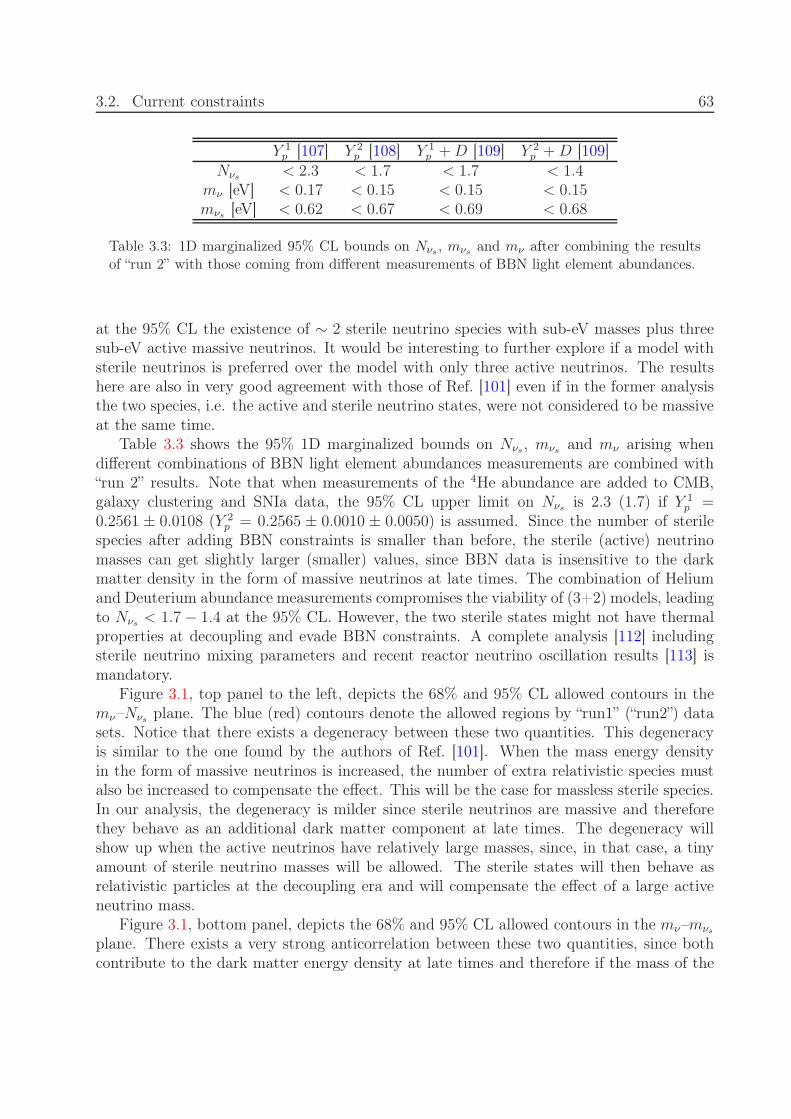
3.2. Current constraints 63
Y 1p [107] Y 2
p [108] Y 1p +D [109] Y 2
p +D [109]Nνs < 2.3 < 1.7 < 1.7 < 1.4
mν [eV] < 0.17 < 0.15 < 0.15 < 0.15mνs [eV] < 0.62 < 0.67 < 0.69 < 0.68
Table 3.3: 1D marginalized 95% CL bounds on Nνs , mνs and mν after combining the resultsof “run 2” with those coming from different measurements of BBN light element abundances.
at the 95% CL the existence of ∼ 2 sterile neutrino species with sub-eV masses plus threesub-eV active massive neutrinos. It would be interesting to further explore if a model withsterile neutrinos is preferred over the model with only three active neutrinos. The resultshere are also in very good agreement with those of Ref. [101] even if in the former analysisthe two species, i.e. the active and sterile neutrino states, were not considered to be massiveat the same time.
Table 3.3 shows the 95% 1D marginalized bounds on Nνs, mνs and mν arising whendifferent combinations of BBN light element abundances measurements are combined with“run 2” results. Note that when measurements of the 4He abundance are added to CMB,galaxy clustering and SNIa data, the 95% CL upper limit on Nνs is 2.3 (1.7) if Y 1
p =0.2561 ± 0.0108 (Y 2
p = 0.2565 ± 0.0010 ± 0.0050) is assumed. Since the number of sterilespecies after adding BBN constraints is smaller than before, the sterile (active) neutrinomasses can get slightly larger (smaller) values, since BBN data is insensitive to the darkmatter density in the form of massive neutrinos at late times. The combination of Heliumand Deuterium abundance measurements compromises the viability of (3+2) models, leadingto Nνs < 1.7 − 1.4 at the 95% CL. However, the two sterile states might not have thermalproperties at decoupling and evade BBN constraints. A complete analysis [112] includingsterile neutrino mixing parameters and recent reactor neutrino oscillation results [113] ismandatory.
Figure 3.1, top panel to the left, depicts the 68% and 95% CL allowed contours in themν–Nνs plane. The blue (red) contours denote the allowed regions by “run1” (“run2”) datasets. Notice that there exists a degeneracy between these two quantities. This degeneracyis similar to the one found by the authors of Ref. [101]. When the mass energy densityin the form of massive neutrinos is increased, the number of extra relativistic species mustalso be increased to compensate the effect. This will be the case for massless sterile species.In our analysis, the degeneracy is milder since sterile neutrinos are massive and thereforethey behave as an additional dark matter component at late times. The degeneracy willshow up when the active neutrinos have relatively large masses, since, in that case, a tinyamount of sterile neutrino masses will be allowed. The sterile states will then behave asrelativistic particles at the decoupling era and will compensate the effect of a large activeneutrino mass.
Figure 3.1, bottom panel, depicts the 68% and 95% CL allowed contours in the mν–mνs
plane. There exists a very strong anticorrelation between these two quantities, since bothcontribute to the dark matter energy density at late times and therefore if the mass of the

64Chapter 3. Constraints on massive sterile neutrino species from current and future
cosmological data
sterile neutrino states grows, the mass of the active ones must decrease. The situation isanalogous to that of QCD thermal axions and massive (active) neutrinos, see Ref. [71].
The top panel to the right of Fig. 3.1 depicts the 68% and 95% CL allowed contours inthe Nνs–mνs plane. In this case, the larger the sterile neutrino mass is, the lower its thermalabundance must be, as expected.
mν
Nν s
0 0.1 0.2 0.3 0.4 0.50
0.5
1
1.5
2
2.5
3
3.5
4
4.5
5
Nνs
mν s
0 1 2 3 4 50
0.1
0.2
0.3
0.4
0.5
mν
mν s
0 0.1 0.2 0.3 0.4 0.50
0.1
0.2
0.3
0.4
0.5
0.6
Figure 3.1: The top and bottom panels show the 68% and 95% CL constraints on the planemν-Nνs , mν-mνs and mνs-Nνs , respectively. The blue (red) contours denote the allowed regionsby “run1” (“run2”) data sets, see text for details. The masses of the sterile and active neutrinosare both in eV units.
3.3 Future constraints
We present here the constraints on the neutrino sector parameters explored in this work fromfuture CMB and galaxy survey measurements, making use of the Fisher matrix formalism,

3.3. Future constraints 65
see also Ref. [114] for a recent analysis. We also compute the potential shifts in the differentcosmological parameters when the sterile neutrino parameters are neglected in the analysis.
3.3.1 Methodology
The Fisher matrix is defined as the expectation value of the second derivative of the likeli-hood surface about the maximum. As long as the posterior distribution for the param-eters is well approximated by a multivariate Gaussian function, its elements are givenby [115, 116, 117]
Fαβ =1
2Tr[
C−1C,αC−1C,β
]
, (3.2)
where C = S + N is the total covariance which consists of signal S and noise N terms.The commas in Eq. (3.2) denote derivatives with respect to the cosmological parameterswithin the assumed fiducial cosmology. Our fiducial model is a ΛCDM cosmology withfive parameters: the physical baryon and CDM densities, ωb = Ωbh
2 and ωc = Ωch2, the
scalar spectral index, ns, h (being the Hubble constant H0 = 100 h km Mpc−1s−1) and thedimensionless amplitude of the primordial curvature perturbations, As (see Tab. 3.4 for theirvalues). Furthermore, we add to the ΛCDM fiducial cosmology three additional parametersfor the neutrino sector: the mass of active neutrinos mν , the mass of sterile neutrinos mνs
and the number of sterile neutrino species Nνs. Notice that, for simplicity, we have keptfixed the reionization optical depth τ since it has no impact on large scale structure data andwe do not expect a strong degeneracy between τ and the neutrino parameters, see Ref. [118].We assume that both active and sterile neutrinos have a degenerate spectrum and that thesterile species are fully thermalized. The fiducial values of the neutrino parameters are listedas well in Tab. 3.4, and they are based on the constraints from current data presented inthe previous section, from which we conclude that mν = 0.1 eV, mνs ≤ 0.5 and Nνs = 1, 2are within the allowed regions for these parameters.
Ωbh2 Ωch
2 ns h As mν [eV] mνs [eV] Nνs
0.02267 0.1131 0.96 0.705 2.64 · 10−9 0.1 0.1-0.5 1-2
Table 3.4: Values of the parameters in the fiducial models explored in this study.
We compute the CMB Fisher matrix to obtain forecasts for the Planck satellite [119].We follow here the method of Ref. [120], considering the likelihood function for a realisticexperiment with partial sky coverage, and noisy data
−2 lnL =∑
ℓ
(2ℓ+ 1)
fBBsky ln
(
CBBℓ
CBBℓ
)
+√
fTTskyf
EEsky ln
(
CTTℓ C
EEℓ − (CTE
ℓ )2
CTTℓ CEE
ℓ − (CTEℓ )2
)
+√
fTTskyf
EEsky
CTTℓ C
EEℓ + C
TTℓ C
EEℓ − 2CTE
ℓ CTEℓ
CTTℓ CEE
ℓ − (CTEℓ )2
+ fBBsky
CBBℓ
CBBℓ
− 2√
fTTskyf
EEsky
−fBBsky
, (3.3)
66Chapter 3. Constraints on massive sterile neutrino species from current and future
cosmological data
and compute its second derivatives to obtain the corresponding Fisher matrix
FCMBαβ =
⟨
− ∂2L∂pα∂pβ
⟩
|p=p . (3.4)
In Eq. (3.3) CXYℓ = CXY
ℓ +NXYℓ with CXY
ℓ the temperature and polarization power spectra(X, Y ≡ T,E,B) and Nℓ the noise bias. Finally, fXY
sky is the fraction of observed skywhich can be different for the T -, E-, and B-modes.
For the galaxy redshift survey Fisher matrix, we follow the prescription of Ref. [121].Assuming the likelihood function for the band powers of a galaxy redshift survey to beGaussian, the Fisher matrix can be approximated as:
F LSSαβ =
∫ ~kmax
~kmin
∂ lnPgg(~k)
∂pα
∂ lnPgg(~k)
∂pβVeff(~k)
d~k
2(2π)3(3.5)
=
∫ 1
−1
∫ kmax
kmin
∂ lnPgg(k, µ)
∂pα
∂ lnPgg(k, µ)
∂pβVeff(k, µ)
2πk2dkdµ
2(2π)3,
where Veff is the effective volume of the survey:
Veff(k, µ) =
[
nP (k, µ)
nP (k, µ) + 1
]2
Vsurvey, (3.6)
µ being the cosine of the angle between the vector along the line of sight and ~k and n beingthe galaxy number density, which is assumed to be constant throughout the survey. Thelinear redshift-space galaxy power spectrum Pgg is related to the real-space linear powerdark matter spectrum Pdm as
Pgg(k) = Pdm(k)(b+ fµ2)2 (3.7)
where b is the bias relating galaxy to dark matter overdensities in real space and f is thelinear growth factor. Both the bias and the growth factor are assumed to vary in eachredshift bin and are considered as additional parameters in the Fisher analysis of galaxysurvey data.
We consider here two redshift surveys: the BOSS (Baryon Oscillation SpectroscopicSurvey) [35] and the Euclid [122, 123] experiments. For the BOSS survey we assume asky area of 10000 deg2, a redshift range of 0.15 < z < 0.65 and a mean galaxy density of2.66×10−4. For Euclid we consider an area of 20000 deg2, a redshift range of 0.15 < z < 1.95and a mean galaxy density of 1.56 × 10⁻³. We divide the surveys in redshift bins of width∆z = 0.1 (a value that is much larger than standard redshift spectroscopic errors), set kmax
to be 0.1h/Mpc and kmin to be greater than 2π/∆V 1/3, where ∆V is the volume of theredshift shell.
Combining the Planck and redshift survey Fisher matrices (Fαβ = F LSSαβ +FCMB
αβ ) we getthe joint constraints for Ωbh
2, Ωch2, ns, H0, As, mν , mνs and Nνs, after marginalizing over
the bias b and the growth factor f . The 1–σ error on parameter pα marginalized over theother parameters is σ(pα) =
√
(F−1)αα, F−1 being the inverse of the Fisher matrix.
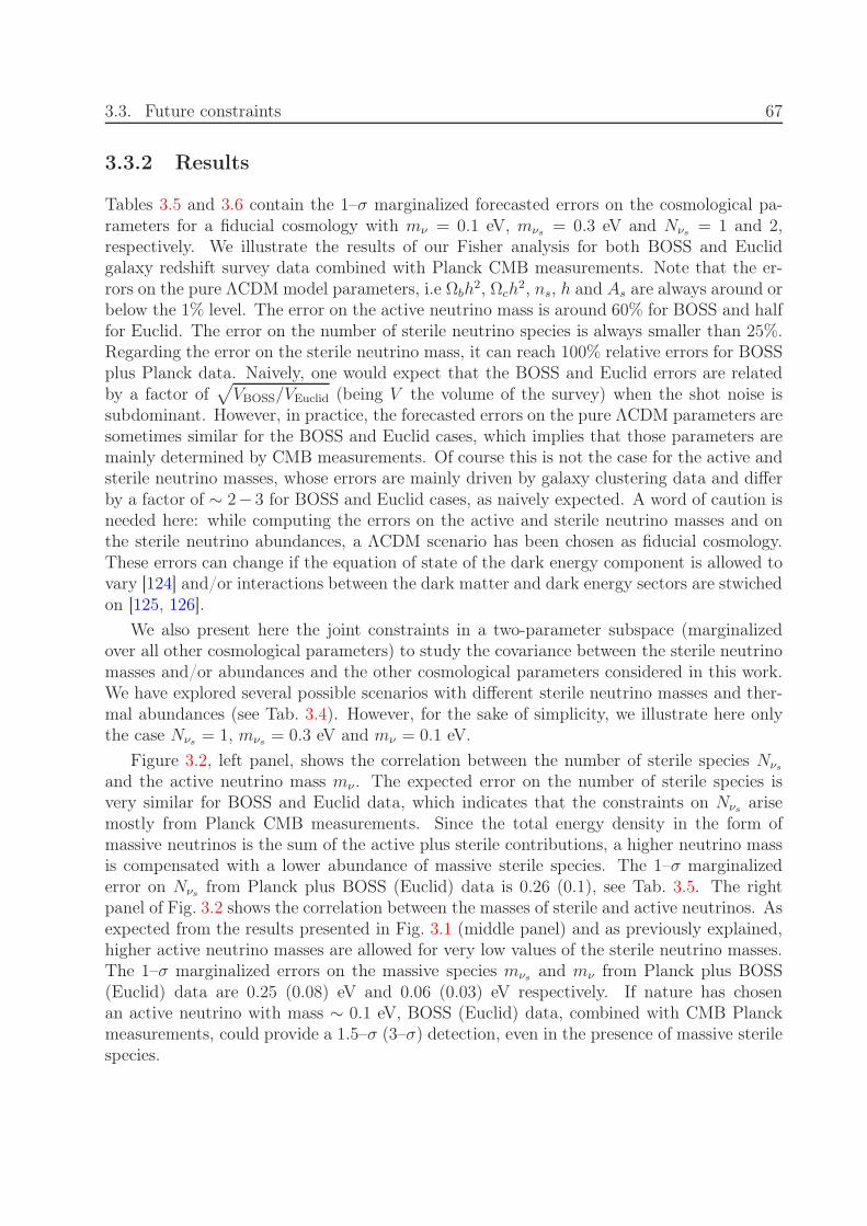
3.3. Future constraints 67
3.3.2 Results
Tables 3.5 and 3.6 contain the 1–σ marginalized forecasted errors on the cosmological pa-rameters for a fiducial cosmology with mν = 0.1 eV, mνs = 0.3 eV and Nνs = 1 and 2,respectively. We illustrate the results of our Fisher analysis for both BOSS and Euclidgalaxy redshift survey data combined with Planck CMB measurements. Note that the er-rors on the pure ΛCDM model parameters, i.e Ωbh
2, Ωch2, ns, h and As are always around or
below the 1% level. The error on the active neutrino mass is around 60% for BOSS and halffor Euclid. The error on the number of sterile neutrino species is always smaller than 25%.Regarding the error on the sterile neutrino mass, it can reach 100% relative errors for BOSSplus Planck data. Naively, one would expect that the BOSS and Euclid errors are relatedby a factor of
√
VBOSS/VEuclid (being V the volume of the survey) when the shot noise issubdominant. However, in practice, the forecasted errors on the pure ΛCDM parameters aresometimes similar for the BOSS and Euclid cases, which implies that those parameters aremainly determined by CMB measurements. Of course this is not the case for the active andsterile neutrino masses, whose errors are mainly driven by galaxy clustering data and differby a factor of ∼ 2− 3 for BOSS and Euclid cases, as naively expected. A word of caution isneeded here: while computing the errors on the active and sterile neutrino masses and onthe sterile neutrino abundances, a ΛCDM scenario has been chosen as fiducial cosmology.These errors can change if the equation of state of the dark energy component is allowed tovary [124] and/or interactions between the dark matter and dark energy sectors are stwichedon [125, 126].
We also present here the joint constraints in a two-parameter subspace (marginalizedover all other cosmological parameters) to study the covariance between the sterile neutrinomasses and/or abundances and the other cosmological parameters considered in this work.We have explored several possible scenarios with different sterile neutrino masses and ther-mal abundances (see Tab. 3.4). However, for the sake of simplicity, we illustrate here onlythe case Nνs = 1, mνs = 0.3 eV and mν = 0.1 eV.
Figure 3.2, left panel, shows the correlation between the number of sterile species Nνs
and the active neutrino mass mν . The expected error on the number of sterile species isvery similar for BOSS and Euclid data, which indicates that the constraints on Nνs arisemostly from Planck CMB measurements. Since the total energy density in the form ofmassive neutrinos is the sum of the active plus sterile contributions, a higher neutrino massis compensated with a lower abundance of massive sterile species. The 1–σ marginalizederror on Nνs from Planck plus BOSS (Euclid) data is 0.26 (0.1), see Tab. 3.5. The rightpanel of Fig. 3.2 shows the correlation between the masses of sterile and active neutrinos. Asexpected from the results presented in Fig. 3.1 (middle panel) and as previously explained,higher active neutrino masses are allowed for very low values of the sterile neutrino masses.The 1–σ marginalized errors on the massive species mνs and mν from Planck plus BOSS(Euclid) data are 0.25 (0.08) eV and 0.06 (0.03) eV respectively. If nature has chosenan active neutrino with mass ∼ 0.1 eV, BOSS (Euclid) data, combined with CMB Planckmeasurements, could provide a 1.5–σ (3–σ) detection, even in the presence of massive sterilespecies.

68Chapter 3. Constraints on massive sterile neutrino species from current and future
cosmological data
Parameter BOSS+PLANCK EUCLID+PLANCKΩbh
2 0.7% 0.3%Ωch
2 2.9% 1.3%ln (1010As) 0.7% 0.4%
h [km/s/Mpc] 1.4% 0.7%ns 0.6% 0.3%
mν [eV] 63.1% 28.0%mνs [eV] 83.2% 26.2%Nνs 25.9% 10.6%
Table 3.5: 1σ marginalized relative errors for a fiducial cosmology with Nνs=1, mν=0.1 eV andmνs=0.3 eV.
Parameter BOSS+PLANCK EUCLID+PLANCKΩbh
2 0.7% 0.3%Ωch
2 1.5% 1.7%ln (1010As) 0.4% 0.4%
h [km/s/Mpc] 1.4% 0.8%ns 0.5% 0.4%
mν [eV] 64.9% 35.9%mνs [eV] 41.9% 16.4%Nνs 10.2% 7.5%
Table 3.6: 1–σ marginalized relative errors for all parameters for a Nνs=2, mν=0.1 eV andmνs=0.3 eV fiducial cosmology.
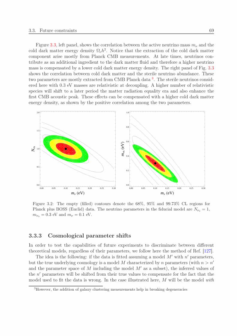
3.3. Future constraints 69
Figure 3.3, left panel, shows the correlation between the active neutrino mass mν and thecold dark matter energy density Ωch
2. Notice that the extraction of the cold dark mattercomponent arise mostly from Planck CMB measurements. At late times, neutrinos con-tribute as an additional ingredient to the dark matter fluid and therefore a higher neutrinomass is compensated by a lower cold dark matter energy density. The right panel of Fig. 3.3shows the correlation between cold dark matter and the sterile neutrino abundance. Thesetwo parameters are mostly extracted from CMB Planck data 3. The sterile neutrinos consid-ered here with 0.3 eV masses are relativistic at decoupling. A higher number of relativisticspecies will shift to a later period the matter radiation equality era and also enhance thefirst CMB acoustic peak. These effects can be compensated with a higher cold dark matterenergy density, as shown by the positive correlation among the two parameters.
æ
0.00 0.05 0.10 0.15 0.20 0.25 0.30
0.0
0.5
1.0
1.5
2.0
mΝ HeVL
NΝs
æ
0.00 0.05 0.10 0.15 0.20 0.25 0.30
0.0
0.2
0.4
0.6
0.8
1.0
mΝ HeVL
mΝsHe
VL
Figure 3.2: The empty (filled) contours denote the 68%, 95% and 99.73% CL regions forPlanck plus BOSS (Euclid) data. The neutrino parameters in the fiducial model are Nνs = 1,mνs = 0.3 eV and mν = 0.1 eV.
3.3.3 Cosmological parameter shifts
In order to test the capabilities of future experiments to discriminate between differenttheoretical models, regardless of their parameters, we follow here the method of Ref. [127].
The idea is the following: if the data is fitted assuming a model M ′ with n′ parameters,but the true underlying cosmology is a model M characterized by n parameters (with n > n′
and the parameter space of M including the model M ′ as a subset), the inferred values ofthe n′ parameters will be shifted from their true values to compensate for the fact that themodel used to fit the data is wrong. In the case illustrated here, M will be the model with
3However, the addition of galaxy clustering measurements help in breaking degeneracies

70Chapter 3. Constraints on massive sterile neutrino species from current and future
cosmological data
æ
0.00 0.05 0.10 0.15 0.20 0.25 0.30 0.35
0.100
0.105
0.110
0.115
0.120
0.125
mΝ HeVL
Wch
2
æ
0.0 0.5 1.0 1.5 2.0
0.100
0.105
0.110
0.115
0.120
0.125
NΝsW
ch2
Figure 3.3: The empty (filled) contours denote the 68%, 95% and and 99.73% CL regions forPlanck plus BOSS (Euclid) data. The neutrino parameters in the fiducial model are Nνs = 1,mνs = 0.3 eV and mν = 0.1 eV.
massive sterile neutrinos and M ′ the one without massive sterile neutrinos. While the firstn′ parameters are the same for both models, the remaining n − n′ = p parameters in theenlarged model M are accounting for the presence of massive sterile neutrinos, i.e. mνs andNνs. Assuming a gaussian likelihood, the shifts of the remaining n′ parameters is given by[127]:
δθ′α = −(F ′−1)αβGβζδψζ α, β = 1 . . . n′, ζ = n′ + 1 . . . n , (3.8)
where F ′ represents the Fisher sub-matrix for the model M ′ without massive steriles and Gdenotes the Fisher matrix for the model M with mνs , Nνs > 0.
We have computed the shifts induced in the cosmological parameters in several truecosmologies with a number of sterile neutrinos Nνs = 1, 2 of masses mνs = 0.1, 0.3 and0.5 eV. The mass of the active neutrino has been kept to 0.1 eV. These cosmologies arethen wrongly fitted to a cosmology without sterile massive neutrino species. While certainparameters are exclusively measured by CMB probes or by the combination of CMB andother cosmological data sets (like Ωch
2, Ωbh2, ns and As), there are other parameters such
as the Hubble constant H0 or the active neutrino mass mν which can be determined byother experiments. Then it is possible to verify the cosmological model assumptions bycomparing the values of H0 and mν extracted from CMB and LSS cosmological data to thevalues of these parameters obtained by other experiments, as missions devoted to measurethe Hubble constant and tritium beta decay experiments 4. The former experiments measure
4Neutrinoless double beta decay provides also a bound on the so-called effective neutrino mass 〈m〉 ≡|∑i U2
eimi|. However, these bounds apply only in the case that neutrinos have a Majorana nature. There-fore, we focus on tritium beta decay constraints which apply regardless of the Dirac vs Majorana nature ofthe neutrino.
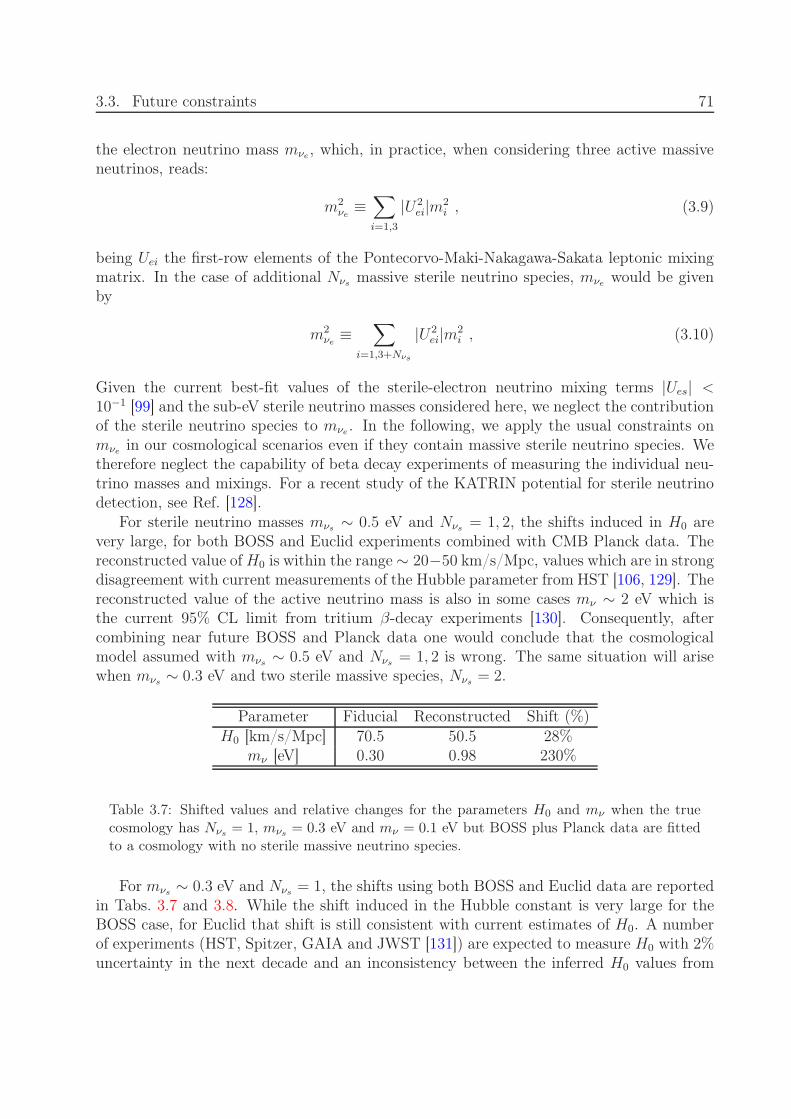
3.3. Future constraints 71
the electron neutrino mass mνe, which, in practice, when considering three active massiveneutrinos, reads:
m2νe
≡∑
i=1,3
|U2ei|m2
i , (3.9)
being Uei the first-row elements of the Pontecorvo-Maki-Nakagawa-Sakata leptonic mixingmatrix. In the case of additional Nνs massive sterile neutrino species, mνe would be givenby
m2νe
≡∑
i=1,3+Nνs
|U2ei|m2
i , (3.10)
Given the current best-fit values of the sterile-electron neutrino mixing terms |Ues| <10−1 [99] and the sub-eV sterile neutrino masses considered here, we neglect the contributionof the sterile neutrino species to mνe . In the following, we apply the usual constraints onmνe in our cosmological scenarios even if they contain massive sterile neutrino species. Wetherefore neglect the capability of beta decay experiments of measuring the individual neu-trino masses and mixings. For a recent study of the KATRIN potential for sterile neutrinodetection, see Ref. [128].
For sterile neutrino masses mνs ∼ 0.5 eV and Nνs = 1, 2, the shifts induced in H0 arevery large, for both BOSS and Euclid experiments combined with CMB Planck data. Thereconstructed value ofH0 is within the range ∼ 20−50 km/s/Mpc, values which are in strongdisagreement with current measurements of the Hubble parameter from HST [106, 129]. Thereconstructed value of the active neutrino mass is also in some cases mν ∼ 2 eV which isthe current 95% CL limit from tritium β-decay experiments [130]. Consequently, aftercombining near future BOSS and Planck data one would conclude that the cosmologicalmodel assumed with mνs ∼ 0.5 eV and Nνs = 1, 2 is wrong. The same situation will arisewhen mνs ∼ 0.3 eV and two sterile massive species, Nνs = 2.
Parameter Fiducial Reconstructed Shift (%)H0 [km/s/Mpc] 70.5 50.5 28%
mν [eV] 0.30 0.98 230%
Table 3.7: Shifted values and relative changes for the parameters H0 and mν when the truecosmology has Nνs = 1, mνs = 0.3 eV and mν = 0.1 eV but BOSS plus Planck data are fittedto a cosmology with no sterile massive neutrino species.
For mνs ∼ 0.3 eV and Nνs = 1, the shifts using both BOSS and Euclid data are reportedin Tabs. 3.7 and 3.8. While the shift induced in the Hubble constant is very large for theBOSS case, for Euclid that shift is still consistent with current estimates of H0. A numberof experiments (HST, Spitzer, GAIA and JWST [131]) are expected to measure H0 with 2%uncertainty in the next decade and an inconsistency between the inferred H0 values from

72Chapter 3. Constraints on massive sterile neutrino species from current and future
cosmological data
Parameter Fiducial Reconstructed Shift (%)H0 [km/s/Mpc] 70.5 65.0 8%
mν [eV] 0.30 0.48 60%
Table 3.8: Shifted values and relative changes for the parameters H0 and mν when the truecosmology has Nνs = 1, mνs = 0.3 eV and mν = 0.1 eV but Euclid plus Planck data are fittedto a cosmology with no sterile massive neutrino species.
these experiments and those from the cosmological probes considered here could point to theexistence of additional sterile neutrino species. On the other hand, the aim of the tritiumbeta decay experiment KATRIN [132] is a sensitivity of mνe < 0.2 eV at 90% CL in caseof a null result or a 5σ discovery potential for mνe ≥ 0.35 eV. Therefore, the reconstructedvalues of mν = 0.48 eV (Euclid plus Planck) and 0.98 eV (BOSS plus Planck) could beeasily testable by the KATRIN experiment. Similar results are obtained for smaller sterileneutrino masses mνs ∼ 0.1 eV with a higher number of sterile species Nνs = 2.
For smaller sterile neutrino masses mνs ∼ 0.1 eV and Nνs = 1, the shift induced in H0 islarger than 2% for both BOSS and Euclid data (combined with Planck). Therefore it wouldstill be possible to check the fiducial cosmology with future measurements of H0. The shiftinduced on the active neutrino mass using Euclid data is negligible and this means that itwould be possible to recover the true value of the active neutrino mass even if the data isfitted to the wrong cosmology. Thus, the combination of Planck and Euclid data would notlead to an inconsistency between active neutrino mass estimates from Planck and Euclid onthe one hand, and beta decay experiments on the other hand. Regarding BOSS plus Planckdata however, the shift induced in the active neutrino mass mν is of the order of 100% andthe comparison with an independent measurement of mν as that performed by KATRINcould test the validity of the cosmological model assumptions.
We have shown above that if the true Nνs = 1, 2, wrongfully assuming Nνs = 0 wouldlead to discrepancies between the cosmological probes considered here (large scale structureand CMB) and independent measurements of H0 and mν . Of course, another clear indicatorthat the assumed model is incorrect is simply that the Nνs = 0 would likely provide a bad fitto the large scale structure and CMB data themselves. However, the induced bias discussedabove would provide a useful extra check when independent measurements of H0 and/or mν
are available. In addition, the bias calculation shows that even if one is not interested in thesterile neutrinos per se, not taking them into account could lead to very wrong conclusionsabout the other cosmological parameters.
3.4 Summary
Neutrino oscillation experiments have brought to light the first departure from the StandardModel of particle physics, indicating that neutrinos have non zero masses and opening thepossibility for a number of extra sterile neutrinos. LSND and MiniBooNE antineutrino
3.4. Summary 73
data require these extra sterile species to be massive. Much effort has been devoted in theliterature to constrain the so called (3+1) (three active plus one sterile) and (3+2) (threeactive plus two sterile) models.
Cosmology can set bounds on both the active and sterile neutrino masses as well as onthe number of sterile neutrino species. We have explored here the current constraints onthese parameters in the most natural scenario which corresponds to the case in which boththe active and sterile neutrinos are massive particles. We find that models with two massivesub-eV sterile neutrinos plus three sub-eV active states are perfectly allowed at the 95% CLby current Cosmic Microwave Background, galaxy clustering and Supernovae Ia data. Thebounds derived here were obtained in the context of a ΛCDM cosmology and other scenarioswith a dark energy component could allow for larger neutrino masses and/or abundances.We have also shown that Big Bang Nucleosynthesis Helium-4 and deuterium abundancesexclude (3+2) models at the 95% CL. However, the extra sterile states do not necessarilyneed to feature thermal abundances at decoupling. Their precise abundances are related totheir mixings with the active neutrinos in the early universe.
We have also forecasted the errors on the active and sterile neutrino parameters fromPlanck and galaxy survey data. Future cosmological data are expected to measure sub-eVactive and sterile neutrino masses and sterile abundances with 10− 30% precision, for sub-eV (0.5 eV> mνs > 0.1 eV) sterile neutrino masses. We have also shown that the presenceof massive sterile neutrinos in the universe could be inferred from inconsistencies amongthe values of H0 obtained from cosmic microwave and galaxy clustering probes and thosearising from independent measurements of the Hubble constant over the next decade. Thevalidity of the cosmological assumptions could also be tested by comparing cosmologicalmeasurements of the active neutrino mass with those obtained from tritium beta decayexperiments.

74Chapter 3. Constraints on massive sterile neutrino species from current and future
cosmological data
Chapter 4
New Neutrino Mass Bounds from Sloan
Digital Sky Survey III Data Release 8
Photometric Luminous Galaxies
In this Chapter we derive neutrino mass bounds from the angular power spectra from theSloan Digital Sky Survey III Data Release Eight (SDSS DR8) sample of photometric galaxieswith CMASS selection criteria. This Chapter is a copy of the paper:
New Neutrino Mass Bounds from Sloan Digital Sky Survey III Data Release 8 Photomet-ric Luminous Galaxies, Roland de Putter, Olga Mena, Elena Giusarma, Shirley Ho, AntonioCuesta, Hee-Jong Seo, Ashley J. Ross & Martin White et al., Astrophys. J. 761, 12 (2012).
4.1 Introduction
During the last several years, experiments involving solar, atmospheric, reactor and acceler-ator neutrinos have adduced robust evidence for flavor change, implying non-zero neutrinomass, see Ref. [89] and references therein. The most economical description of the neutrinooscillation phenomena requires at least two massive neutrino mass eigenstates to explain thetwo mass differences1, ∆m2
12 = 7.59 · 10−5 eV2 and ∆m223 = 2.5 · 10−3 eV2 [56, 133], which
drive the solar and atmospheric transitions. Despite the remarkable success of past andpresent oscillation experiments, and the promising prospects for future searches, the indi-vidual neutrino masses and the Dirac versus Majorana neutrino character are key questionsthat continue to be unanswered by oscillation experiments.
Direct information on the absolute scale of neutrino masses can be extracted from kine-matical studies of weak decays producing neutrinos. The present upper bound on theelectron-neutrino mass from tritium beta-decay experiments is 2 eV (95% confidence level(CL)) [58, 134], and in the future the KATRIN experiment is expected to be sensitive toelectron-neutrino masses approaching 0.2 eV (90% CL) [130]. Searches for the Majorana
1Neutrino oscillations are described by mass squared differences and not by the absolute values of themass eigenstates
75
76Chapter 4. New Neutrino Mass Bounds from Sloan Digital Sky Survey III Data Release 8
Photometric Luminous Galaxies
neutrino nature involve neutrinoless double beta decay ββ(0ν), a rare and as yet unobservedtransition between two nuclei. Observational upper limits on ββ(0ν) rates provide an upperbound on the so-called effective Majorana mass of the electron neutrino, 〈meff〉 < 0.3−1.0 eV,bound which would only apply if neutrinos are Majorana particles [61]. Forthcoming ββ(0ν)experiments aim for sensitivity approaching 〈meff〉 < 0.05 eV [61].
Cosmology provides one of the means to tackle the absolute scale of neutrino masses.Some of the earliest cosmological bounds on neutrino masses followed from the requirementthat massive relic neutrinos, present today in the expected numbers, do not saturate thecritical density of the Universe, i.e., that the neutrino mass energy density given by
Ων =
∑
mν
93.1h2eV(4.1)
satisfies Ων ≤ 1. The Universe therefore offers a new laboratory for testing neutrino massesand neutrino physics. Accurate measurements of the Cosmic Microwave Background (CMB)temperature and polarization anisotropy from satellite, balloon-borne and ground-based ex-periments have fully confirmed the predictions of the standard cosmological model andallow us to weigh neutrinos [84]. Indeed, neutrinos can play a relevant role in large-scalestructure formation and leave key signatures in several cosmological data sets. More specif-ically, the amount of primordial relativistic neutrinos changes the epoch of matter-radiationequality, leaving an imprint on CMB anisotropies. After becoming non-relativistic, theirfree-streaming nature damps power on small scales, suppressing the growth of matter den-sity fluctuations and thus affecting both the CMB and galaxy clustering observables in thelow-redshift universe [84]. Measurements of all of these observations have been used to placenew bounds on neutrino physics from cosmology [135, 136, 137, 138, 139, 140, 141, 142, 143,144, 124, 145, 146, 147, 148, 149, 105, 91, 150, 90, 151, 152, 153], with a current limit onthe sum of neutrino masses Σmν
<∼ 0.6 eV at 95% CL (e.g. [105]), depending on the precisecombination of data sets and on the underlying cosmological model.
We present here neutrino mass bounds from the final imaging data set of the Sloan DigitalSky Survey (SDSS-III) [32], using the photometric redshift catalog of Ross et al. [36]. Weconsider the CMASS sample [37] of luminous galaxies of SDSS DR8 [40], the eighth datarelease of SDSS and the first data release of the Baryon Oscillation Spectroscopic Survey(BOSS) [35], with photometric redshifts z = 0.45 − 0.65. This sample covers an area ofapproximately 10,000 square degrees and consists of 900,000 galaxies. It is thus the largestsample of luminous galaxies so far and promises strong constraints on the neutrino properties(see [150] for an analysis of a slightly smaller SDSS photometric sample).
We derive neutrino constraints from the angular power spectra of the galaxy density atdifferent redshifts, in combination with priors from the CMB and from measurements of theHubble parameter, supernovae distances and the BAO scale. The spectra and the analysisof a minimal ΛCDM cosmology are described in detail in [154] and the measurement of theBAO scale from the spectra is presented in [155]. We will often refer to these works fordetails and focus here on the neutrino bound.
The structure of the paper is as follows. In section 6.3, we describe the data set and thederived angular spectra. We then discuss our theoretical model for the spectra and their
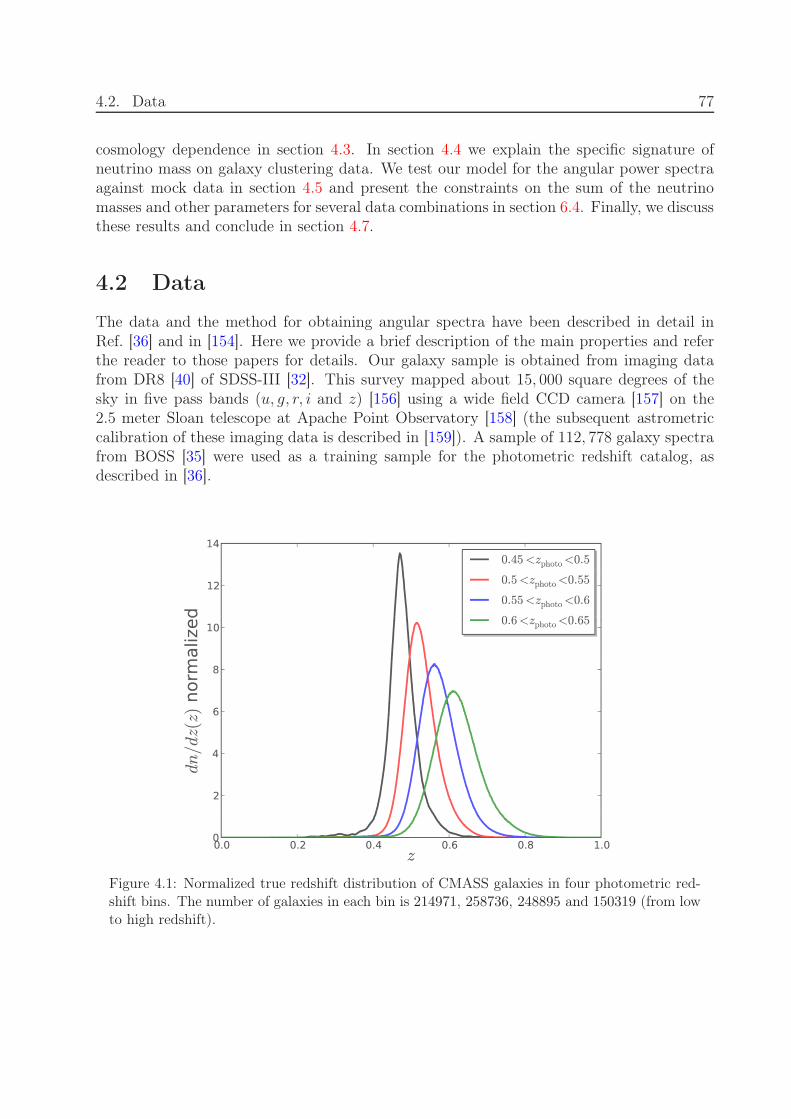
4.2. Data 77
cosmology dependence in section 4.3. In section 4.4 we explain the specific signature ofneutrino mass on galaxy clustering data. We test our model for the angular power spectraagainst mock data in section 4.5 and present the constraints on the sum of the neutrinomasses and other parameters for several data combinations in section 6.4. Finally, we discussthese results and conclude in section 4.7.
4.2 Data
The data and the method for obtaining angular spectra have been described in detail inRef. [36] and in [154]. Here we provide a brief description of the main properties and referthe reader to those papers for details. Our galaxy sample is obtained from imaging datafrom DR8 [40] of SDSS-III [32]. This survey mapped about 15, 000 square degrees of thesky in five pass bands (u, g, r, i and z) [156] using a wide field CCD camera [157] on the2.5 meter Sloan telescope at Apache Point Observatory [158] (the subsequent astrometriccalibration of these imaging data is described in [159]). A sample of 112, 778 galaxy spectrafrom BOSS [35] were used as a training sample for the photometric redshift catalog, asdescribed in [36].
Figure 4.1: Normalized true redshift distribution of CMASS galaxies in four photometric red-shift bins. The number of galaxies in each bin is 214971, 258736, 248895 and 150319 (from lowto high redshift).
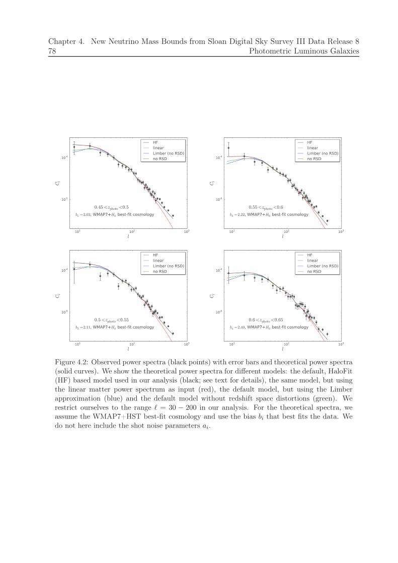
78Chapter 4. New Neutrino Mass Bounds from Sloan Digital Sky Survey III Data Release 8
Photometric Luminous Galaxies
Figure 4.2: Observed power spectra (black points) with error bars and theoretical power spectra(solid curves). We show the theoretical power spectra for different models: the default, HaloFit(HF) based model used in our analysis (black; see text for details), the same model, but usingthe linear matter power spectrum as input (red), the default model, but using the Limberapproximation (blue) and the default model without redshift space distortions (green). Werestrict ourselves to the range ℓ = 30 − 200 in our analysis. For the theoretical spectra, weassume the WMAP7+HST best-fit cosmology and use the bias bi that best fits the data. Wedo not here include the shot noise parameters ai.
4.3. Modeling the angular power spectra 79
We focus on the approximately stellar mass-limited CMASS sample of luminous galaxies,detailed in [37], which are divided into four photometric redshift bins, zphoto = 0.45 −0.5 − 0.55 − 0.6 − 0.65. The photometric redshift error lies in the range σz(z) = 0.04 −0.06, increasing from low to high redshift. Figure 4.1 shows the estimated true redshiftdistribution of each bin, determined using the methods described in section 5.3 of [36].
The calculation of the angular power spectrum for each bin is described in detail in [154]and uses the optimal quadratic estimator (OQE) method outlined in [160, 161, 162, 163].The four power spectra are binned in ℓ space with a typical wave band width of ∆ℓ = 10.The expectation value of the power spectrum in a wave band is a convolution of the truepower spectrum with a window function of width roughly equal to the typical wave bandwidth. Examples of these window functions are shown in Fig. 3 of [155]. When fitting thedata to the underlying theoretical model, we always apply these window functions to thetheoretical power spectra before calculating the likelihood relative to the data.
The four power spectra are plotted with their error bars in Fig. 4.2. The solid curvesrepresent theoretical power spectra based on several assumptions. These power spectrawill be discussed in detail in section 4.3. Since the low ℓ wave bands are more prone tosystematics [36], we are conservative and do not consider bands with ℓ < 30 in our analysis.We shall apply cuts at ℓmax = 150 and 200 in order to suppress uncertainties from non-linear corrections to the modeled power spectra, as discussed in the following sections. Themedian redshift (z ≈ 0.55) contributions to these maximum angular modes arise from three-dimensional modes with wave vectors k ≈ 0.10hMpc−1 and k ≈ 0.14hMpc−1, respectively.We thus use 17 (12) data points per redshift slice for ℓmax = 200 (150).
4.3 Modeling the angular power spectra
The galaxy overdensity in the i-th redshift bin can be expanded in terms of spherical har-monics,
δ(i)g (n) =
∑
ℓm
a(i)ℓm Yℓm(n) , (4.2)
so that the angular power (and cross) spectra are defined as
〈a(i)ℓma
(j)∗ℓ′m′〉 ≡ C
(ij)ℓ δK
ℓℓ′ δKmm′ , (4.3)
where δKij is the Kronecker delta function. As mentioned in the previous section, we do not
estimate our spectra by directly transforming the observed density field to harmonics space,but use instead the optimal quadratic estimator technique. To constrain the sum of theneutrino masses and other cosmological parameters, the observed spectra are compared toa cosmology dependent model, which we now describe.
The galaxy overdensity on the sky is a line-of-sight projection of the three-dimensionalredshift space galaxy overdensity δg(d(z) n, z),
δ(i)g (n) =
∫
dz gi(z)(
δg(d(z) n, z) − (H(z))−1n · ∇(n · v(d(z) n, z))
)
, (4.4)
80Chapter 4. New Neutrino Mass Bounds from Sloan Digital Sky Survey III Data Release 8
Photometric Luminous Galaxies
where
gi(z) =dni/dz(z)
∫
dz′ dni/dz(z′)(4.5)
is the normalized redshift distribution of galaxies in bin i (with dni/dz(z) the numberof galaxies per steradian per unit redshift), d(z) is the comoving distance to redshift z(assuming a flat universe) and v is the galaxy velocity field. The velocity term arises becausegradients of the peculiar velocity contribution to the distance in redshift space change thevolume, and consequently, the number density2.
We assume a linear, scale-independent bias for the galaxy density,
δg(x, z) = bg(z) δm(x, z) , (4.6)
with δm the matter overdensity. For the peculiar velocity field, we use the continuity equationin the linear regime, which gives for a Fourier mode with wave vector k,
v = −ıβ(z)δg(k)k
k2, (4.7)
where β(z) = f(z)/bg(z) is the redshift distortion parameter and
f(z) ≡ d lnD(z)
d ln a(4.8)
is the growth factor (with D(z) the linear growth function). In the presence of neutrinos, thegrowth function is no longer scale independent at late time as the neutrinos suppress growthon scales below the free streaming length [164, 165], but not on larger scales (with a broadtransition regime in between). We shall ignore the scale dependent growth in β(z) since itis a small (≪ 10%) correction to the already small effect (on the scales of interest here)of redshift space distortions (RSD, see Fig. 4.2). However, this scale-dependent growth isincluded in the real space power spectrum, as this is the main signature of massive neutrinos.
We simplify our treatment of the galaxy bias adding four free parameters bi to describethe bias in each bin. The results from our simulations barely change when considering abias bg(z) that varies within redshift bins, showing that this is a safe approximation3. Itthen follows from the above (see [166, 167, 163]) that
C(ii)ℓ = b2i
2
π
∫
k2dk Pm(k, z = 0)(
∆(i)ℓ (k) + ∆
RSD,(i)ℓ (k)
)2
, (4.9)
where Pm(k, z = 0) is the matter power spectrum at redshift zero and
∆(i)ℓ (k) =
∫
dz gi(z)T (k, z) jℓ(k d(z)) . (4.10)
2Instead of writing the projected galaxy overdensity as an integral over the observed redshift (includingpeculiar velocity contributions) as in Eq. (4.4), one could equivalently do the integral over “true” cosmicredshift, see Ref. [163], in which case only the true three-dimensional galaxy overdensity appears explicitlyand the redshift space distortions come in through a modification of the distribution gi(z).
3A similar approach is considered to model β(z), appearing in the redshift space distortion contribution.
For each bin we calculate an effective growth rate fi = (ΩDM(zi))0.56
where zi is the mean redshift of thei-th bin, ignoring the scale dependence of the RSD growth.
4.3. Modeling the angular power spectra 81
Here, jℓ is the spherical Bessel function and T (k, z) the matter transfer function relative toredshift zero4. The contribution due to redshift space distortions is
∆RSD,(i)l (k) = βi
∫
dz gi(z)T (k, z)
[
(2l2 + 2l − 1)
(2l + 3)(2l− 1)jl(kd(z))
− l(l − 1)
(2l − 1)(2l + 1)jl−2(kd(z))
− (l + 1)(l + 2)
(2l + 1)(2l + 3)jl+2(kd(z))
]
. (4.11)
To compute the matter power spectrum at a given redshift Pm(k, z) = Pm(k, z =0)T 2(k, z), we first make use of the CAMB code [82], which provides the linear powerspectrum by integrating the Boltzmann equations of all species including massive neutrinos.We then apply the HaloFit prescription5 [168] to the linear power spectrum to account fornon-linear effects on the matter power spectrum.
While in the linear regime the galaxy spectrum is easy to model, calculations on non-linear scales inevitably have large uncertainties. This effect is aggravated by the presenceof massive neutrinos since for the massive neutrino case the non-linear regime has beenexplored less extensively in the literature than for a vanilla ΛCDM model. In the non-linear regime, the matter power spectrum receives corrections due to gravitational collapse,the galaxy bias becomes scale-dependent, and redshift space distortions receive importantcontributions from velocity dispersion in collapsed objects. We take into account non-linearcorrections to the matter spectrum using HaloFit. The effect of non-linearities on redshiftspace distortions at the relevant scales here is small as it is largely washed out by line-of-sight projection. However, we do expect significant corrections to our model on small scalesdue to non-linear galaxy bias, which we address below.
For angular scales where non-linear effects cannot be ignored, the contribution to a givenangular mode ℓ from a redshift z comes exclusively from three-dimensional modes withwave vector k ≈ ℓ/d(z). Clearly, to avoid large non-linear corrections, the analysis must berestricted to low ℓ. On the other hand, the density of modes per unit ℓ increases with ℓso we want to use as many modes as possible without biasing the results. Figure 4.3 (leftpanel) depicts (as a function of redshift z) the value of ℓ above which non-linear correctionsto the three-dimensional power spectrum contributions to the angular spectrum becomeimportant (i.e. ℓNL ≡ kNL(z) d(z)), considering various assumptions for the non-linear scalekNL(z). Given that most of our signal is produced in the range z = 0.45−0.65, and assumingthat our model becomes inadequate at k > 0.15hMpc−1, we conclude that a conservativechoice would be ℓmax somewhere between 150 and 200.
Alternatively, we can obtain an indication of the importance of non-linear galaxy biasby considering the effect of non-linear corrections to the matter power spectrum6 (which we
4The transfer function is defined as δm(k, z) = T (k, z) δm(k, z = 0).5Recently, [169] developed an extension to HaloFit that incorporates the effect of massive neutrinos. We
do not use this prescription as the correction to standard HaloFit is negligible on the scales of our interest.6However, one must keep in mind that this may underestimate the effect of non-linear galaxy bias, as
galaxies are more strongly clustered than matter and are thus prone to larger non-linear corrections.
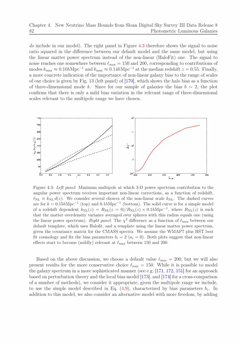
82Chapter 4. New Neutrino Mass Bounds from Sloan Digital Sky Survey III Data Release 8
Photometric Luminous Galaxies
do include in our model). The right panel in Figure 4.3 therefore shows the signal to noiseratio squared in the difference between our default model and the same model, but usingthe linear matter power spectrum instead of the non-linear (HaloFit) one. The signal tonoise reaches one somewhere between ℓmax = 150 and 200, corresponding to contributions ofmodes kmax ≈ 0.10hMpc−1 and kmax ≈ 0.14hMpc−1 at the median redshift z = 0.55. Finally,a more concrete indication of the importance of non-linear galaxy bias to the range of scalesof our choice is given by Fig. 13 (left panel) of [170], which shows the halo bias as a functionof three-dimensional mode k. Since for our sample of galaxies the bias b ∼ 2, the plotconfirms that there is only a mild bias variation in the relevant range of three-dimensionalscales relevant to the multipole range we have chosen.
Figure 4.3: Left panel: Minimum multipole at which 3-D power spectrum contribution to theangular power spectrum receives important non-linear corrections, as a function of redshift,ℓNL ≡ kNL d(z). We consider several choices of the non-linear scale kNL. The dashed curvesare for k = 0.15hMpc−1 (top) and 0.1hMpc−1 (bottom). The solid curve is for a simple modelof a redshift dependent kNL(z) = RNL(z = 0)/RNL(z) × 0.1hMpc−1, where RNL(z) is suchthat the matter overdensity variance averaged over spheres with this radius equals one (usingthe linear power spectrum). Right panel: The χ2 difference as a function of ℓmax between ourdefault template, which uses Halofit, and a template using the linear matter power spectrum,given the covariance matrix for the CMASS spectra. We assume the WMAP7 plus HST bestfit cosmology and fix the bias parameters bi = 2 (ai = 0). Both plots suggest that non-lineareffects start to become (mildly) relevant at ℓmax between 150 and 200.
Based on the above discussion, we choose a default value ℓmax = 200, but we will alsopresent results for the more conservative choice ℓmax = 150. While it is possible to modelthe galaxy spectrum in a more sophisticated manner (see e.g. [171, 172, 151] for an approachbased on perturbation theory and the local bias model [173], and [174] for a cross-comparisonof a number of methods), we consider it appropriate, given the multipole range we include,to use the simple model described in Eq. (4.9), characterized by bias parameters bi. Inaddition to this model, we also consider an alternative model with more freedom, by adding

4.4. Cosmological Signature of Neutrinos 83
shot noise-like parameters ai,
C(ii)ℓ = b2i
2
π
∫
k2dk Pm(k, z = 0)(
∆(i)ℓ (k) + ∆
RSD,(i)ℓ (k)
)2
+ ai . (4.12)
The parameters ai serve to mimic effects of scale-dependent galaxy bias and to model theeffect of potential insufficient shot noise subtraction. This model is a version of what issometimes referred to as the “P-model” (e.g. [175, 174]) and is independently motivated bythe halo model [176, 177, 178, 179] and the local bias ansatz [180, 181, 172]. We furtherdiscuss the validity of the parameterizations with and without ai in section 4.5.
Figure 4.2 shows the theoretical galaxy spectra as described in this section. The errorbars follow from the optimal quadratic estimator method used to construct the power spectra(see [154] for details). Comparing the spectra with (black) and without (green) redshift spacedistortions shows that this effect is negligible for ℓ > 50 and is probably not relevant forthe range of scales we use in our data analysis, i.e. ℓ > 30. Although we never employ it,we also show the effect of using the Limber approximation [182] and find that for ℓ > 30 itworks excellently.
4.4 Cosmological Signature of Neutrinos
In the analysis presented in this paper we assume that there are three species of massiveneutrinos with equal masses mν . Massive neutrinos affect galaxy formation at scales belowthe Hubble horizon when they become non relativistic,
knr ≃ 0.0145( mν
1 eV
)
√
ΩDM hMpc−1 , (4.13)
with ΩDM the present total dark matter energy density, i.e. cold dark matter plus massiveneutrinos, relative to the critical density. The non-relativistic neutrino overdensities clusterat a given redshift z only at scales where the wavenumber of perturbations is below theneutrino free streaming scale
kfs(z) =0.677
(1 + z)1/2
( mν
1 eV
)
√
ΩDM hMpc−1 , (4.14)
due to the pressure gradient, which prevents gravitational clustering. On spatial scales largerthan the free streaming scale k < kfs, neutrinos cluster and behave as cold dark matter (andbaryons). Perturbations with comoving wavenumber larger than the free streaming scalecan not grow due to the large neutrino velocity dispersion. As a consequence, the growthrate of density perturbations decreases and the matter power spectrum is suppressed atk > kfs. Since the free streaming scale depends on the individual neutrino masses and noton their sum, a measurement of kfs could, in principle, provide the ordering of the neutrinomass spectrum. In practice, such a task appears extremely challenging, see [183].
Figure 4.4 illustrates the effect of massive neutrinos on the angular power spectra. Thesolid curves depict the results for the four redshift bins exploited here in the case of a
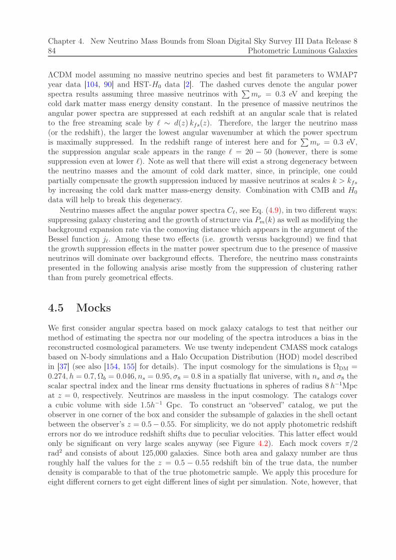
84Chapter 4. New Neutrino Mass Bounds from Sloan Digital Sky Survey III Data Release 8
Photometric Luminous Galaxies
ΛCDM model assuming no massive neutrino species and best fit parameters to WMAP7year data [104, 90] and HST-H0 data [2]. The dashed curves denote the angular powerspectra results assuming three massive neutrinos with
∑
mν = 0.3 eV and keeping thecold dark matter mass energy density constant. In the presence of massive neutrinos theangular power spectra are suppressed at each redshift at an angular scale that is relatedto the free streaming scale by ℓ ∼ d(z) kfs(z). Therefore, the larger the neutrino mass(or the redshift), the larger the lowest angular wavenumber at which the power spectrumis maximally suppressed. In the redshift range of interest here and for
∑
mν = 0.3 eV,the suppression angular scale appears in the range ℓ = 20 − 50 (however, there is somesuppression even at lower ℓ). Note as well that there will exist a strong degeneracy betweenthe neutrino masses and the amount of cold dark matter, since, in principle, one couldpartially compensate the growth suppression induced by massive neutrinos at scales k > kfs
by increasing the cold dark matter mass-energy density. Combination with CMB and H0
data will help to break this degeneracy.Neutrino masses affect the angular power spectra Cℓ, see Eq. (4.9), in two different ways:
suppressing galaxy clustering and the growth of structure via Pm(k) as well as modifying thebackground expansion rate via the comoving distance which appears in the argument of theBessel function jℓ. Among these two effects (i.e. growth versus background) we find thatthe growth suppression effects in the matter power spectrum due to the presence of massiveneutrinos will dominate over background effects. Therefore, the neutrino mass constraintspresented in the following analysis arise mostly from the suppression of clustering ratherthan from purely geometrical effects.
4.5 Mocks
We first consider angular spectra based on mock galaxy catalogs to test that neither ourmethod of estimating the spectra nor our modeling of the spectra introduces a bias in thereconstructed cosmological parameters. We use twenty independent CMASS mock catalogsbased on N-body simulations and a Halo Occupation Distribution (HOD) model describedin [37] (see also [154, 155] for details). The input cosmology for the simulations is ΩDM =0.274, h = 0.7,Ωb = 0.046, ns = 0.95, σ8 = 0.8 in a spatially flat universe, with ns and σ8 thescalar spectral index and the linear rms density fluctuations in spheres of radius 8 h−1Mpcat z = 0, respectively. Neutrinos are massless in the input cosmology. The catalogs covera cubic volume with side 1.5h−1 Gpc. To construct an “observed” catalog, we put theobserver in one corner of the box and consider the subsample of galaxies in the shell octantbetween the observer’s z = 0.5− 0.55. For simplicity, we do not apply photometric redshifterrors nor do we introduce redshift shifts due to peculiar velocities. This latter effect wouldonly be significant on very large scales anyway (see Figure 4.2). Each mock covers π/2rad2 and consists of about 125,000 galaxies. Since both area and galaxy number are thusroughly half the values for the z = 0.5 − 0.55 redshift bin of the true data, the numberdensity is comparable to that of the true photometric sample. We apply this procedure foreight different corners to get eight different lines of sight per simulation. Note, however, that

4.5. Mocks 85
Figure 4.4: Effect of neutrinos on the angular power spectra. The solid and dashed curvesdepict the massless and Σmν = 0.3 eV cases, respectively.
these lines of sight are not completely independent as they are based on the same simulationvolume. Finally, for each line of sight, we average the spectra over all twenty independentrealizations in order to increase the signal to noise ratio. The covariance matrix for themock angular power spectrum is rescaled accordingly to reflect the decrease in covariancedue to taking the average.
As described in section 4.3, we consider a model characterized by the cosmological pa-rameters and a galaxy bias b0 (giving our mock bin the label 0), and a more conservativemodel with bias b0 and nuisance parameter a0, so that the spectrum is given by
C(00)ℓ = b20
2
π
∫
k2dk Pm(k, z = 0)(
∆(i)ℓ (k)
)2
+ a0 . (4.15)
In the galaxy bias-only version, a0 is simply set to zero.As a direct test of this model, we fit it to the averaged mock spectrum. In this first
approach, we keep the cosmology fixed to the mock’s input cosmology and restrict the fitto the range ℓ = 30− 200. The only free parameters are thus either b0 or (b0, a0). We use a

86Chapter 4. New Neutrino Mass Bounds from Sloan Digital Sky Survey III Data Release 8
Photometric Luminous Galaxies
Figure 4.5: Example of an averaged mock spectrum (green points with error bars) and theoret-ical spectra (solid lines). Fixing the cosmology to the mock input cosmology (see text), we fitthe averaged mock spectrum in the range ℓ = 30−200 to our model described in the text. Theblack curve is the resulting best-fit spectrum if we only fit a (scale-independent) galaxy biasb0 (best-fit value b0 = 2.02), while the red curve is the best fit in a model that also includesthe nuisance parameter a0 (best fit values b0 = 2.00, a0 = 1.05 · 10−6). To provide a hint ofthe importance of non-linear effects in this multipole range, we plot the spectrum based on alinear three dimensional matter power spectrum in blue (b0 = 2.02, a0 = 0)
modification of the publicly available COSMOMC package [103] to sample this parameterspace using Monte Carlo Markov Chains (MCMC). We show the resulting best-fit spectratogether with the mock average in Fig. 4.5. Considering first the default, galaxy bias-only model (black curve), we find that the best fit to the mock result has a linear biasb0 = 2.02 (with uncertainty σ(b0) < 0.01) and has χ2 = 11.3. This should be comparedto an expectation value of 〈χ2〉 = 16 based on 17 data bins and one free parameter. Thegalaxy bias model thus provides a good fit to the simulated spectrum (the probability ofgetting a χ2 lower than 11.3 for an expectation value of 16 is approximately 20%).
Next, including the shot noise-like parameter a0 to take into account potential resid-

4.5. Mocks 87
ual shot noise and/or non-linear effects not captured by our simple Halofit plus scale-independent galaxy bias model, we find a best fit model with a0 = 1.1 · 10−6 and b0 = 2.00.However, the uncertainty in a0 is σ(a0) = 1.0 · 10−6 so the preference for a non-zero valuecannot be considered significant. In this model, we find χ2 = 10.1, to be compared to theexpected 〈χ2〉 = 15. This is only a marginal (∆χ2 ≈ 1.2) improvement.
Restricting the fitting range to ℓ = 30−150, we find ∆χ2 = 1.1 between the two best-fitmodels, and a0 = (1.8 ± 1.9) × 10−6.
Figure 4.6: Left panel: Recovered values of ΩDMh2 from averaged mock spectrum togetherwith CMB prior. We consider spectra from eight different lines of sight. The points with errorbars show the posterior mean values and 1σ error bars after the Monte Carlo analysis for twoscenarios: varying Σmν with (red) and without (blue) a0 marginalized. The vertical magentalines indicate the input value ΩDMh2 = 0.11166 (solid) and the input ± one and two σ, whereσ = 0.0032 is the parameter uncertainty based on the data set WMAP7+HST+angular spectra(ai = 0 fixed). There is a bias of about 1σ without the nuisance parameter, which disappearswhen ai is marginalized over. Right panel: The posterior neutrino mass distributions for thetwo cases discussed above. The mock constraints are consistent with the input cosmology ofΣmν = 0. Other parameters are all reconstructed to close to their input values and are notstrongly affected by the angular spectra.
The comparison above suggests that for the range ℓ = 30 − 200, the galaxy bias modelwithout an extra nuisance parameter may be sufficient. We now undertake a more completecheck of our model and the entire cosmology analysis by using MCMC to fit the full spaceof cosmological parameters as well as the galaxy bias (and shot noise parameter) to theaveraged mock spectrum. The differences between the resulting best-fit parameter valuesand the “true”, i.e. input, values give an indication of the parameter bias introduced by ourmethod. To break parameter degeneracies, while not letting the prior bias us away from theinput cosmology, we include a “mock” CMB prior7, which will provide a likelihood similar
7 The “mock” CMB prior is defined by χ2WMAP7 ≡ (pi − pi,input)COV−1
ij (pj − p,input), where pi are theparameters at each point of the chain, pi,input the input parameters, COVij is the WMAP7 covariancematrix and i, j are summed over.
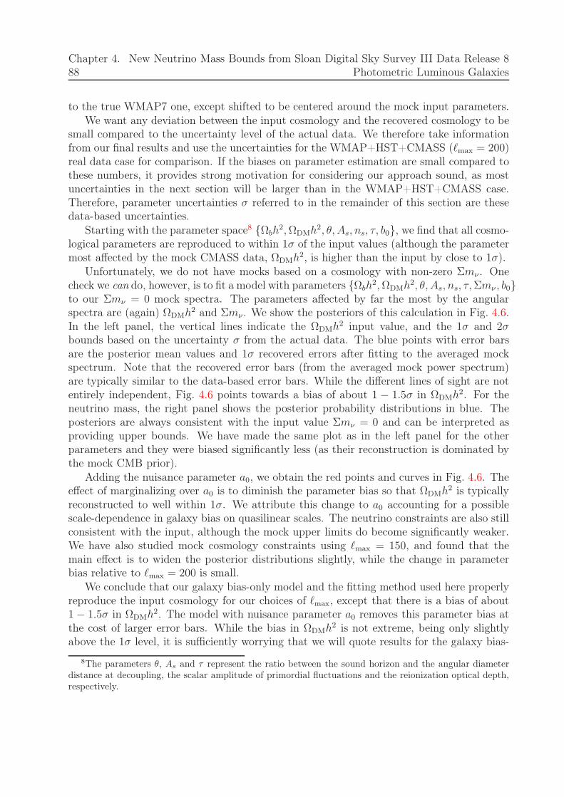
88Chapter 4. New Neutrino Mass Bounds from Sloan Digital Sky Survey III Data Release 8
Photometric Luminous Galaxies
to the true WMAP7 one, except shifted to be centered around the mock input parameters.We want any deviation between the input cosmology and the recovered cosmology to be
small compared to the uncertainty level of the actual data. We therefore take informationfrom our final results and use the uncertainties for the WMAP+HST+CMASS (ℓmax = 200)real data case for comparison. If the biases on parameter estimation are small compared tothese numbers, it provides strong motivation for considering our approach sound, as mostuncertainties in the next section will be larger than in the WMAP+HST+CMASS case.Therefore, parameter uncertainties σ referred to in the remainder of this section are thesedata-based uncertainties.
Starting with the parameter space8 Ωbh2,ΩDMh
2, θ, As, ns, τ, b0, we find that all cosmo-logical parameters are reproduced to within 1σ of the input values (although the parametermost affected by the mock CMASS data, ΩDMh
2, is higher than the input by close to 1σ).Unfortunately, we do not have mocks based on a cosmology with non-zero Σmν . One
check we can do, however, is to fit a model with parameters Ωbh2,ΩDMh
2, θ, As, ns, τ,Σmν , b0to our Σmν = 0 mock spectra. The parameters affected by far the most by the angularspectra are (again) ΩDMh
2 and Σmν . We show the posteriors of this calculation in Fig. 4.6.In the left panel, the vertical lines indicate the ΩDMh
2 input value, and the 1σ and 2σbounds based on the uncertainty σ from the actual data. The blue points with error barsare the posterior mean values and 1σ recovered errors after fitting to the averaged mockspectrum. Note that the recovered error bars (from the averaged mock power spectrum)are typically similar to the data-based error bars. While the different lines of sight are notentirely independent, Fig. 4.6 points towards a bias of about 1 − 1.5σ in ΩDMh
2. For theneutrino mass, the right panel shows the posterior probability distributions in blue. Theposteriors are always consistent with the input value Σmν = 0 and can be interpreted asproviding upper bounds. We have made the same plot as in the left panel for the otherparameters and they were biased significantly less (as their reconstruction is dominated bythe mock CMB prior).
Adding the nuisance parameter a0, we obtain the red points and curves in Fig. 4.6. Theeffect of marginalizing over a0 is to diminish the parameter bias so that ΩDMh
2 is typicallyreconstructed to well within 1σ. We attribute this change to a0 accounting for a possiblescale-dependence in galaxy bias on quasilinear scales. The neutrino constraints are also stillconsistent with the input, although the mock upper limits do become significantly weaker.We have also studied mock cosmology constraints using ℓmax = 150, and found that themain effect is to widen the posterior distributions slightly, while the change in parameterbias relative to ℓmax = 200 is small.
We conclude that our galaxy bias-only model and the fitting method used here properlyreproduce the input cosmology for our choices of ℓmax, except that there is a bias of about1 − 1.5σ in ΩDMh
2. The model with nuisance parameter a0 removes this parameter bias atthe cost of larger error bars. While the bias in ΩDMh
2 is not extreme, being only slightlyabove the 1σ level, it is sufficiently worrying that we will quote results for the galaxy bias-
8The parameters θ, As and τ represent the ratio between the sound horizon and the angular diameterdistance at decoupling, the scalar amplitude of primordial fluctuations and the reionization optical depth,respectively.
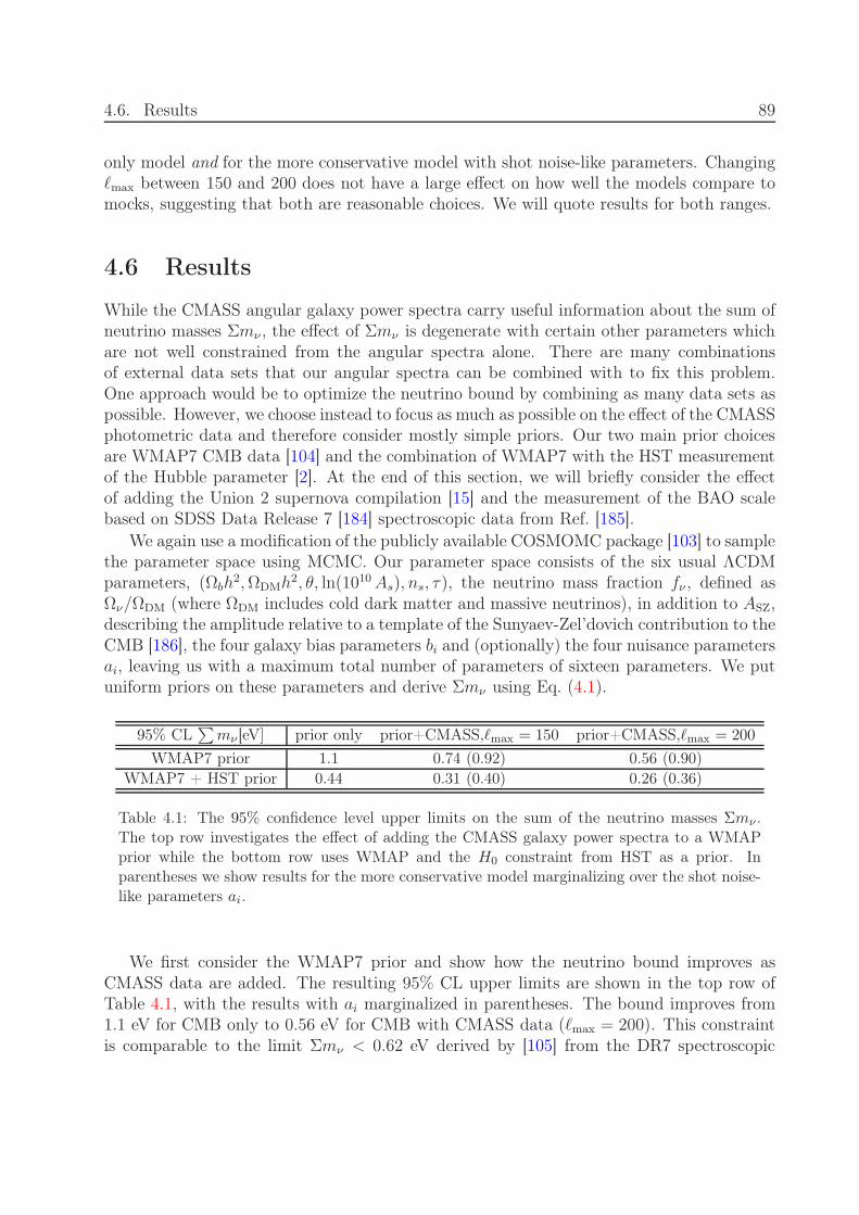
4.6. Results 89
only model and for the more conservative model with shot noise-like parameters. Changingℓmax between 150 and 200 does not have a large effect on how well the models compare tomocks, suggesting that both are reasonable choices. We will quote results for both ranges.
4.6 Results
While the CMASS angular galaxy power spectra carry useful information about the sum ofneutrino masses Σmν , the effect of Σmν is degenerate with certain other parameters whichare not well constrained from the angular spectra alone. There are many combinationsof external data sets that our angular spectra can be combined with to fix this problem.One approach would be to optimize the neutrino bound by combining as many data sets aspossible. However, we choose instead to focus as much as possible on the effect of the CMASSphotometric data and therefore consider mostly simple priors. Our two main prior choicesare WMAP7 CMB data [104] and the combination of WMAP7 with the HST measurementof the Hubble parameter [2]. At the end of this section, we will briefly consider the effectof adding the Union 2 supernova compilation [15] and the measurement of the BAO scalebased on SDSS Data Release 7 [184] spectroscopic data from Ref. [185].
We again use a modification of the publicly available COSMOMC package [103] to samplethe parameter space using MCMC. Our parameter space consists of the six usual ΛCDMparameters, (Ωbh
2,ΩDMh2, θ, ln(1010As), ns, τ), the neutrino mass fraction fν , defined as
Ων/ΩDM (where ΩDM includes cold dark matter and massive neutrinos), in addition to ASZ,describing the amplitude relative to a template of the Sunyaev-Zel’dovich contribution to theCMB [186], the four galaxy bias parameters bi and (optionally) the four nuisance parametersai, leaving us with a maximum total number of parameters of sixteen parameters. We putuniform priors on these parameters and derive Σmν using Eq. (4.1).
95% CL∑
mν [eV] prior only prior+CMASS,ℓmax = 150 prior+CMASS,ℓmax = 200
WMAP7 prior 1.1 0.74 (0.92) 0.56 (0.90)
WMAP7 + HST prior 0.44 0.31 (0.40) 0.26 (0.36)
Table 4.1: The 95% confidence level upper limits on the sum of the neutrino masses Σmν .The top row investigates the effect of adding the CMASS galaxy power spectra to a WMAPprior while the bottom row uses WMAP and the H0 constraint from HST as a prior. Inparentheses we show results for the more conservative model marginalizing over the shot noise-like parameters ai.
We first consider the WMAP7 prior and show how the neutrino bound improves asCMASS data are added. The resulting 95% CL upper limits are shown in the top row ofTable 4.1, with the results with ai marginalized in parentheses. The bound improves from1.1 eV for CMB only to 0.56 eV for CMB with CMASS data (ℓmax = 200). This constraintis comparable to the limit Σmν < 0.62 eV derived by [105] from the DR7 spectroscopic
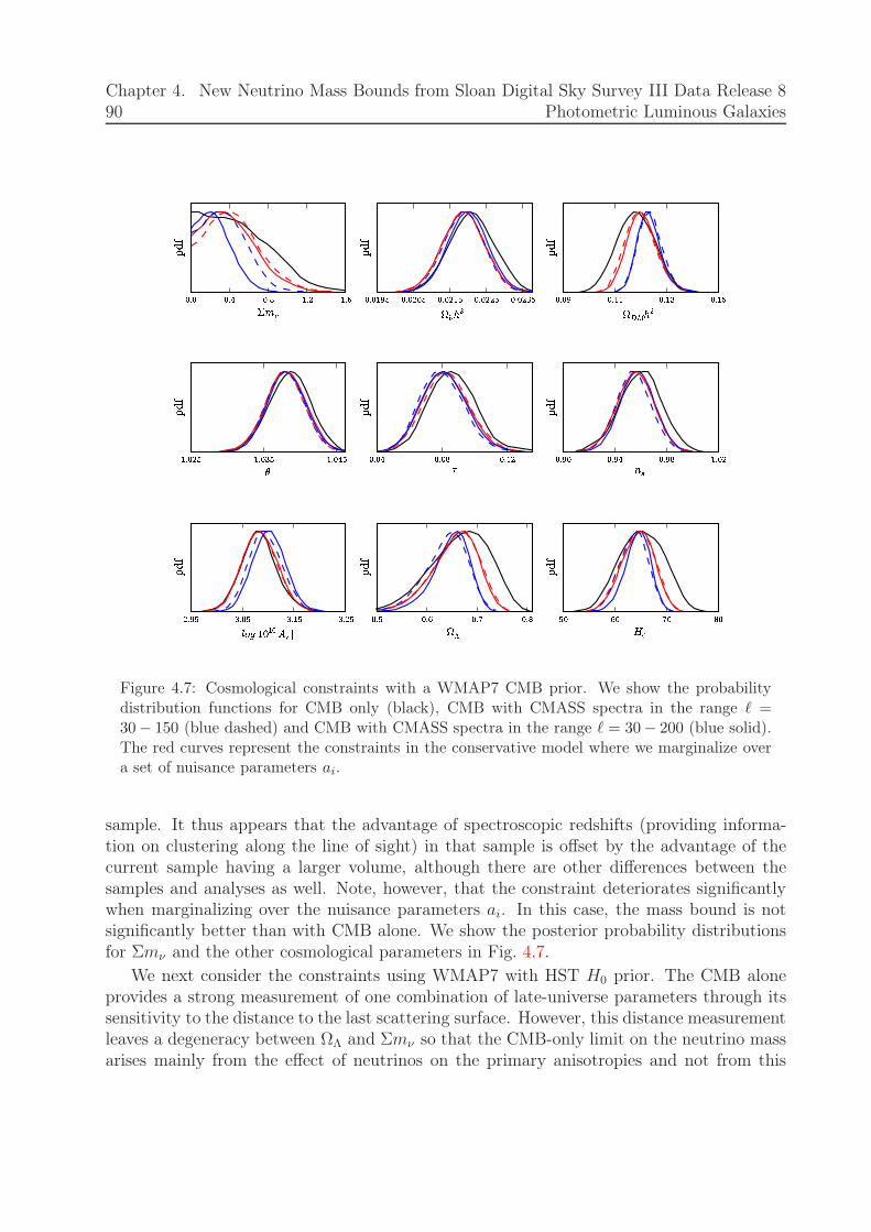
90Chapter 4. New Neutrino Mass Bounds from Sloan Digital Sky Survey III Data Release 8
Photometric Luminous Galaxies
Figure 4.7: Cosmological constraints with a WMAP7 CMB prior. We show the probabilitydistribution functions for CMB only (black), CMB with CMASS spectra in the range ℓ =30− 150 (blue dashed) and CMB with CMASS spectra in the range ℓ = 30− 200 (blue solid).The red curves represent the constraints in the conservative model where we marginalize overa set of nuisance parameters ai.
sample. It thus appears that the advantage of spectroscopic redshifts (providing informa-tion on clustering along the line of sight) in that sample is offset by the advantage of thecurrent sample having a larger volume, although there are other differences between thesamples and analyses as well. Note, however, that the constraint deteriorates significantlywhen marginalizing over the nuisance parameters ai. In this case, the mass bound is notsignificantly better than with CMB alone. We show the posterior probability distributionsfor Σmν and the other cosmological parameters in Fig. 4.7.
We next consider the constraints using WMAP7 with HST H0 prior. The CMB aloneprovides a strong measurement of one combination of late-universe parameters through itssensitivity to the distance to the last scattering surface. However, this distance measurementleaves a degeneracy between ΩΛ and Σmν so that the CMB-only limit on the neutrino massarises mainly from the effect of neutrinos on the primary anisotropies and not from this
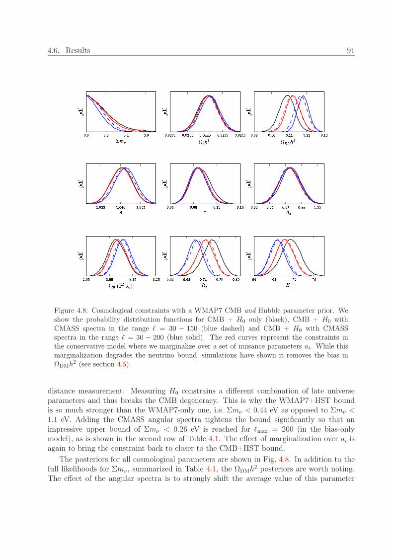
4.6. Results 91
Figure 4.8: Cosmological constraints with a WMAP7 CMB and Hubble parameter prior. Weshow the probability distribution functions for CMB + H0 only (black), CMB + H0 withCMASS spectra in the range ℓ = 30 − 150 (blue dashed) and CMB + H0 with CMASSspectra in the range ℓ = 30 − 200 (blue solid). The red curves represent the constraints inthe conservative model where we marginalize over a set of nuisance parameters ai. While thismarginalization degrades the neutrino bound, simulations have shown it removes the bias inΩDMh2 (see section 4.5).
distance measurement. Measuring H0 constrains a different combination of late universeparameters and thus breaks the CMB degeneracy. This is why the WMAP7+HST boundis so much stronger than the WMAP7-only one, i.e. Σmν < 0.44 eV as opposed to Σmν <1.1 eV. Adding the CMASS angular spectra tightens the bound significantly so that animpressive upper bound of Σmν < 0.26 eV is reached for ℓmax = 200 (in the bias-onlymodel), as is shown in the second row of Table 4.1. The effect of marginalization over ai isagain to bring the constraint back to closer to the CMB+HST bound.
The posteriors for all cosmological parameters are shown in Fig. 4.8. In addition to thefull likelihoods for Σmν , summarized in Table 4.1, the ΩDMh
2 posteriors are worth noting.The effect of the angular spectra is to strongly shift the average value of this parameter
92Chapter 4. New Neutrino Mass Bounds from Sloan Digital Sky Survey III Data Release 8
Photometric Luminous Galaxies
(blue curve), while including the nuisance parameters (red curve) weakens the shift. Thelast two parameters in Fig. 4.8 (and 4.7), ΩΛ and H0, are not independent and can beexpressed in terms of the preceding parameters. The shift thus is really only significant forone independent parameter, ΩDMh
2, in our basis. The results in section 4.5 suggest that theshift in the bias-only case might partially be a bias due to our model and that the resultswith ai marginalized are unbiased.
We do not explicitly show the correlations between parameters, but have verified that,in the CMB+CMASS case, the neutrino mass has its strongest degeneracies with ΩDMh
2,the bias parameters bi and σ8. While, in agreement with our discussion in section 4.4, theinclusion of the Hubble prior removes the Σmν −ΩDMh
2 degeneracy, the strong correlationswith bi and σ8 remain.
We have also added supernova and BAO data to the CMB+HST+CMASS data set,and considered the neutrino mass bound in the bias-only model, but we found negligibleimprovement (from 0.26 eV to 0.25 eV) relative to the case without these additional datasets. These additional data sets do carry significant information, but this information isdegenerate with the information already present in the three default data sets.
For the multipole range ℓ = 30 − 150, we show the results using dashed lines in Figures4.7 and 4.8. The 95% CL upper limit for CMB+HST+CMASS in this case is 0.31(0.40) eVand for CMB+CMASS it is 0.74 (0.92) eV fixing (varying) ai = 0. A significant amount ofinformation is thus contained in the large ℓ range of multipoles, which makes sense as thenumber of modes is large.
Finally, we consider the question of where most of the neutrino mass information comesfrom. In principle, massive neutrinos affect the angular power spectra both by their small-scale suppression of the three-dimensional power spectrum, and by changing the projectionof physical scales onto angular scales through their effect on the background expansion. Asdiscussed in section 4.4, we expect the former effect to carry more constraining power thanthe latter effect. We test this by running Monte Carlo chains where the effect of massiveneutrinos on the three-dimensional power spectrum is artificially taken out, while the effecton the background expansion is left intact. Specifically, we replace the usual linear CAMBpower spectrum by the spectrum given by the Eisenstein and Hu (EH) fitting formula [187],which does not include the effect of massive neutrinos. We find that in this setup, includingthe CMASS galaxy power spectra does not improve the neutrino mass bound relative tothe case with CMB, or with CMB+HST, only. In other words, the projection effect alonecarries little information on neutrino mass (at least after marginalizing over the effectsof other parameters) and the bounds quoted in this manuscript can be attributed to thesmall-scale suppression of the three-dimensional power spectrum.
4.7 Conclusions
We have exploited angular power spectra from the SDSS-III DR8 sample of photometricgalaxies with CMASS selection criteria to put interesting constraints on the sum of neutrinomasses. We have used mock galaxy catalogs based on N-body simulations and HOD mod-
4.7. Conclusions 93
eling to test two models for the angular galaxy spectra. Based on these tests, we decidedto compare the data to theoretical spectra based on the non-linear matter power spectrumaugmented by a linear galaxy bias factor. However, since this model does result in a bias inΩDMh
2 of ∼ 1 − 1.5σ, we have also fitted the data to a more conservative model, with anadditional set of shot noise-like fitting parameters, in which this bias is virtually absent. Thetests also motivated us to use the multipole range ℓ = 30 − 200, but we quoted results forthe more conservative choice ℓ = 30−150 as well. The added advantage is that this analysisprovides insight into the range of scales that yields the galaxy clustering information.
Combining the CMASS data with a CMB prior from the WMAP7 survey, we find anupper bound Σmν < 0.56 eV (0.90 eV) at 95% confidence level for ℓmax = 200 in the modelwith free parameters bi (bi and ai). Adding the HST measurement of the Hubble parameter,the probability distribution tightens and we find Σmν < 0.26 eV (0.36 eV). We have alsoconsidered the effect of adding supernova and a (lower redshift) BAO measurement, butwhen the HST prior is included already, these additions lower the upper limit to 0.25 eV (inthe bias-only model). Considering the dependence on the multipole range, characterized bya maximum multipole ℓmax, we find that a significant amount of information resides in thelargest multipoles ℓ = 150 − 200, but that even for ℓmax = 150, the galaxy spectra place astrong bound on neutrino mass. Our main results are summarized in Table 4.1.
It is interesting to compare these results to the outcome of an analysis of a similar(but smaller) high redshift SDSS photometric catalog, the MegaZ sample [188]. In [150],the strongest bound quoted is a 95% CL upper limit of 0.28 eV, including SN and BAOdata in addition to CMB, HST and MegaZ. However, this particular bound is based ona multipole range with ℓmax = 300 and no nuisance parameters ai. As we have discussedextensively, we believe ℓmax = 200 (or even slightly lower) is a better choice if one wantsto avoid significant, unknown non-linear corrections to the galaxy bias. For this choice, theMegaZ sample yields an upper bound of 0.34 eV. Assuming the aggressive, bias-only model(as in the MegaZ analysis). the value we find for the CMASS sample is 0.25 eV, which isthus a significant improvement. However, it must be kept in mind that this model causes asmall parameter bias and that the more conservative model yields a weaker bound of 0.36eV.
The bounds presented here rule out the quasi-degenerate neutrino mass hierarchy. Forexample, for Σmν = 0.25 eV, it follows from |∆m2
23| = 2.5 ·10−3 eV2 that the mass difference|m3 −m2| ≈ 0.015 eV, so that the largest mass difference is |m3 −m2|/(Σmν/3) ≈ 20% ofthe average neutrino mass. We are thus entering the regime where the mass splittings aresignificant. Looking forward, the prospects are exciting. As the sensitivity of cosmologicalneutrino mass measurements improves, the sum of the masses will either be measured, i.e. avalue that can be distinguished from zero will be found, or the upper limit will be sharpened.However, even in the latter case, interesting things can be learned. If the sum of the massesis found to be less than ∼ 0.1eV, this rules out the inverted hierarchy, leaving the normalhierarchy as the only option. Moreover, even in the normal hierarchy, Σmν is not allowedto be lower than ∼ 0.05eV so that sooner or later a measurement, rather than an upperbound, can be expected.
Finally, we note that BOSS is currently taking spectra for a sample of galaxies with the
94Chapter 4. New Neutrino Mass Bounds from Sloan Digital Sky Survey III Data Release 8
Photometric Luminous Galaxies
same selection criteria as the galaxies considered in this paper and will reach a sample ofapproximately 1, 500, 000 galaxies when finished in 2014. The results presented here arethus only the tip of the iceberg of what can be done with BOSS. The spectroscopic data willallow a measurement of the three-dimensional power spectrum for an even larger volumethan considered here (if the low redshifts sample is included) so that also clustering inthe line-of-sight direction can be resolved, thus promising significantly stronger cosmologyconstraints than from the photometric data.
Chapter 5
Neutrino and Dark Radiation properties
in light of CMB observations
In this Chapter we set new bounds on the dark radiation and neutrino properties in differentcosmological scenarios combining the ACT and SPT data with the nine-year data releaseof the Wilkinson Microwave Anisotropy Probe (WMAP-9), Baryon Acoustic Oscillationdata, Hubble Telescope measurements of the Hubble constant and Supernovae Ia luminositydistance data. This Chapter is a copy of the paper:
Neutrino and Dark Radiation properties in light of latest CMB observations, MariaArchidiacono, Elena Giusarma, Alessandro Melchiorri & Olga Mena, 2013, published inPhysical Review D 87, 103519 (2013),
5.1 Introduction
Solar, atmospheric, reactor, and accelerator neutrinos have provided compelling evidence forthe existence of neutrino oscillations. Barring exotic explanations, oscillation data implynon-zero neutrino masses. However, oscillation experiments only provide bounds on theneutrino mass squared differences, and therefore the measurement of the absolute scaleof the neutrino mass must come from different observations. In the Standard Model ofelementary particles, there are three active neutrinos. However, additional sterile neutrinospecies, or extra relativistic degrees of freedom could also arise in a number of extensionsto the standard model of particle physics, as for instance, in axion models [70, 71], indecaying of non-relativistic matter models [72], in scenarios with gravity waves [73], extradimensions [74, 75, 76], early dark energy [77] or in asymmetric dark matter models [78].Cosmological data provide a tool to test the neutrino properties, since the neutrino massesand abundances affect both the Cosmic Microwave Background (CMB) physics as well asthe galaxy clustering properties, see Refs [93, 94, 100, 99, 91, 92, 101, 189, 87, 94, 190,191, 192, 193, 194, 195, 196, 197] for constraints on the neutrino masses and/or abundanceswith a variety of cosmological data sets and different assumptions regarding the fiducialcosmology.
95

96 Chapter 5. Neutrino and Dark Radiation properties in light of CMB observations
On the other hand, cosmological measurements also allow to test the clustering proper-ties of the extra relativistic degrees of freedom, parameterized via Neff , being Neff = 3.04in the standard model scenario. The clustering pattern of the dark radiation componentis represented by its rest frame speed of sound c2eff and its viscosity parameter c2vis. Theformer parameter controls the relationship between velocity and anisotropic stress, beingthese parameters c2eff = c2vis = 1/3 if the dark radiation background is composed by neutri-nos. Several analyses have set bounds on these parameters [198, 199, 200] under differentassumptions regarding the underlying cosmological model.
Recently new CMB data have become available. The Wilkinson Microwave AnisotropyProbe (WMAP) collaboration has presented the cosmological implications of their finalnine–year data release [18], finding
∑
mν < 0.44 eV at the 95% CL and Neff = 3.84 ± 0.40(being Neff the number of thermalised massless neutrino species) when they combine theirdata with CMB small scale measurements (as those from previous data releases from boththe Atacama Cosmology Telescope ACT [201] and the South Pole Telescope SPT [19]),Baryon Acoustic Oscillations (BAO) and Hubble Space Telescope (HST) measurements.
The SPT collaboration has also recently presented their observations of 2540 deg2 ofsky, providing the CMB temperature anisotropy power over the multipole range 650 < ℓ <3000 [20, 21], corresponding to the region from the third to the ninth acoustic peak. TheSPT measurements have found evidence for a decreasing power at high multipoles relativeto the predictions within a ΛCDM scenario, which suggest, potentially, that extensions tothe minimal ΛCDM scenario might be needed. In the case in which massive neutrinos areadded in the cosmological data analyses, the SPT collaboration finds that the combinationof SPT data with WMAP (7 year data), together with Baryon Acoustic Oscillation (BAO)and Hubble Space Telescope (HST) measurements shows a 2σ preference for these models(when compared to the ΛCDM scenario). In the case of three active massive neutrinos,they find
∑
mν = 0.32 ± 0.11 after considering CMB, BAO, HST and SPT cluster mea-surements. However, if the BAO measurements are removed and only CMB and HST dataare considered, the evidence for neutrino masses disappears at the 95% CL. The authorsof Ref. [20] also find that when a curvature component or a running in the spectral indexof the primordial perturbation spectrum are added as free parameters together with
∑
mν ,the preference for nonzero neutrino masses is significantly reduced. When Neff massless neu-trinos are considered, the bounds are Neff = 3.71± 0.35 for the combination of CMB, BAOand HST data sets. Finally, when allowing for Neff massive neutrino species the bounds are∑
mν = 0.51 ± 0.15 eV and Neff = 3.86 ± 0.37, implying a ∼ 3σ preference for∑
mν > 0and a 2.2σ preference for Neff > 3.046.
These findings, if confirmed by future CMB observations, as those by the ongoing Planckmission [9], have an enormous impact for Majorana neutrino searches. The mean value for∑
mν found by the SPT collaboration implies a quasi-degenerate neutrino spectrum andtherefore the discovery of the neutrino character becomes at reach at near future neutrinolessdouble beta decay experiments [202].
However, and also recently, the ACT collaboration has released new measurements of theCMB damping tail [22], finding a much lower value for Neff = 2.79 ± 0.56 when combiningwith WMAP 7 year data. When considering also BAO and HST measurements, the value

5.2. Data and Cosmological parameters 97
is higher, Neff = 3.50 ± 0.42.The two data sets, SPT and ACT, seem also to disagree in the value of the lensing
amplitude parameter AL at more than 95% CL [203]. On the other hand, ACT data donot seem to see evidence for neutrino masses, placing an upper limit of
∑
mν < 0.39 eV at95% CL when ACT data are combined with WMAP 7 year data together with BAO andHST measurements.
We explore here the cosmological constraints in several neutrino and dark radiationscenarios including the new WMAP 9 year data as well as the new SPT and ACT mea-surements at high multipoles ℓ. We also consider the impact of other cosmological datasets, as BAO, HST and Supernova Ia luminosity distance measurements. We start withthe massive neutrino case within a ΛCDM scenario, setting bounds first on
∑
mν assumingthree massive neutrinos and then moving to the case in which there are Neff massive specieswith a total mass given by
∑
mν . We then enlarge the minimal ΛCDM scenario allowing formore general models with a constant dark energy equation of state or with a running of thescalar spectral index. We continue by studying the dark radiation properties, focusing firston the thermal abundances Neff and adding after the dark radiation clustering propertiesc2vis and c2eff as free parameters in the analysis.
The structure of the paper is as follows. In Sec. 6.3 we describe the data sets used inthe numerical analyses as well as the cosmological parameters used in each of the neutrinoand dark radiation models examined in Sec. 5.3. We draw our conclusions in Sec. 5.4.
5.2 Data and Cosmological parameters
The standard, three massive neutrino scenario we explore here is described by the followingset of parameters:
ωb, ωc,Θs, τ, ns, log[1010As],∑
mν , (5.1)
being ωb ≡ Ωbh2 and ωc ≡ Ωch
2 the physical baryon and cold dark matter energy densities,Θs the ratio between the sound horizon and the angular diameter distance at decoupling,τ is the reionization optical depth, ns the scalar spectral index, As the amplitude of theprimordial spectrum and
∑
mν the sum of the masses of the three active neutrinos in eV.We assume a degenerate neutrino mass spectrum in the following. The former scenario isenlarged with Neff massive neutrinos in the case of extended models
ωb, ωc,Θs, τ, ns, log[1010As], Neff ,∑
mν , (5.2)
or with a constant dark energy equation of state w (or with a running of the scalar spectralindex nrun) when considering more general cosmological models:
ωb, ωc,Θs, τ, ns, log[1010As], w(nrun),∑
mν . (5.3)
We also study dark radiation models, described by ∆Neff relativistic (i.e..massless) degreesof freedom together with three massive neutrinos with
∑
mν = 0.3 eV. This first dark
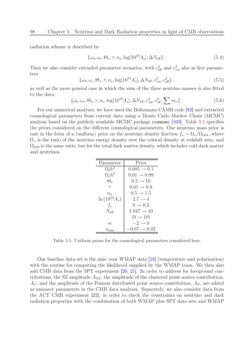
98 Chapter 5. Neutrino and Dark Radiation properties in light of CMB observations
radiation scheme is described by
ωb, ωc,Θs, τ, ns, log[1010As],∆Neff . (5.4)
Then we also consider extended parameter scenarios, with c2eff and c2vis also as free parame-ters:
ωb, ωc,Θs, τ, ns, log[1010As],∆Neff , c2vis, c
2eff , (5.5)
as well as the more general case in which the sum of the three neutrino masses is also fittedto the data:
ωb, ωc,Θs, τ, ns, log[1010As],∆Neff , c2vis, c
2eff ,∑
mν . (5.6)
For our numerical analyses, we have used the Boltzmann CAMB code [82] and extractedcosmological parameters from current data using a Monte Carlo Markov Chain (MCMC)analysis based on the publicly available MCMC package cosmomc [103]. Table 5.1 specifiesthe priors considered on the different cosmological parameters. Our neutrino mass prior iscast in the form of a (uniform) prior on the neutrino density fraction fν = Ων/ΩDM, whereΩν is the ratio of the neutrino energy density over the critical density at redshift zero, andΩDM is the same ratio, but for the total dark matter density, which includes cold dark matterand neutrinos.
Parameter PriorΩbh
2 0.005 → 0.1Ωch
2 0.01 → 0.99Θs 0.5 → 10τ 0.01 → 0.8ns 0.5 → 1.5
ln (1010As) 2.7 → 4fν 0 → 0.2Neff 1.047 → 10
(0 → 10)w −2 → 0nrun −0.07 → 0.02
Table 5.1: Uniform priors for the cosmological parameters considered here.
Our baseline data set is the nine–year WMAP data [18] (temperature and polarization)with the routine for computing the likelihood supplied by the WMAP team. We then alsoadd CMB data from the SPT experiment [20, 21]. In order to address for foreground con-tributions, the SZ amplitude ASZ , the amplitude of the clustered point source contribution,AC , and the amplitude of the Poisson distributed point source contribution, AP , are addedas nuisance parameters in the CMB data analyses. Separately, we also consider data fromthe ACT CMB experiment [22], in order to check the constraints on neutrino and darkradiation properties with the combination of both WMAP plus SPT data sets and WMAP
5.3. Results 99
plus ACT data sets. To the CMB basic data sets we add the latest constraint on the Hubbleconstant H0 from the Hubble Space Telescope (HST) [2], or supernova data from the 3 yearSupernova Legacy Survey (SNLS3), see Ref. [12]. We do not consider the combination ofHST and SNLS3 measurements because these two data sets are not totally independent. Inthe case of SNLS3 data, we add in the MCMC analysis two extra nuisance parameters relatedto the light curve fitting procedure used to analyse the supernova (SN) data. These param-eters characterise the dependence of the intrinsic supernova magnitude on stretch (whichmeasures the shape of the SN light curve) and color [12]. Galaxy clustering measurementsare considered in our analyses via BAO signals. We use here the BAO signal from DR9 [46]of the Baryon Acoustic Spectroscopic Survey (BOSS) [204, 205], with a median redshift ofz = 0.57. Together with the CMASS DR9 data, we also include the recent measurementof the BAO scale based on a re-analysis (using reconstruction [206]) of the LRG samplefrom Data Release 7 with a median redshift of z = 0.35 [43], the measurement of the BAOsignal at a lower redshift z = 0.106 from the 6dF Galaxy Survey 6dFGS [45] and the BAOmeasurements from the WiggleZ Survey at z = 0.44, z = 0.6 and z = 0.73 [44]. The datacombinations for which we will show results in the next section are the following: WMAPand SPT/ACT; WMAP, SPT/ACT and HST; WMAP, SPT/ACT and SNLS3; WMAP,SPT/ACT and BAO; WMAP, SPT/ACT, HST and BAO; and finally WMAP, SPT/ACT,SNLS3 and BAO.
5.3 Results
Here we present the constraints from current cosmological data sets on the neutrino thermalabundance Neff and on the sum of their masses
∑
mν in different scenarios, consideringseparately SPT and ACT CMB data sets.
5.3.1 Standard Cosmology plus massive neutrinos
Through this section we shall assume a ΛCDM cosmology with either three or Neff lightmassive neutrinos. The left panels of Figs. 5.1 and 5.2, depict our results for the threeand Neff massive neutrino assumptions, respectively, in the case of considering SPT CMBdata, combined with the other data sets exploited here. Tables 5.2 and 5.3 present the meanvalues and errors (or 95% CL bounds) in the three and Neff massive neutrino scenarios in thecase of considering SPT for the different data combinations detailed in the previous section.Our results agree with those presented in Ref. [20] by the SPT collaboration. Notice thatBAO data are crucial for the preference for massive neutrinos in the three massive neutrinocase, in which
∑
mν = 0.33 ± 0.17 (∑
mν = 0.40 ± 0.18 eV) for CMB plus BAO plus HST(SNLS3) data. In the Neff massive neutrino scenario, the bounds are
∑
mν = 0.56±0.23 eVand Neff = 4.21± 0.46 (
∑
mν = 0.50± 0.21 eV and Neff = 3.87± 0.68) for CMB plus BAOplus HST (SNLS3) data.
If BAO data are removed, the preference for massive neutrinos disappears in the threemassive neutrino case, with a 95% CL upper limit on the sum of the three active neutrinos
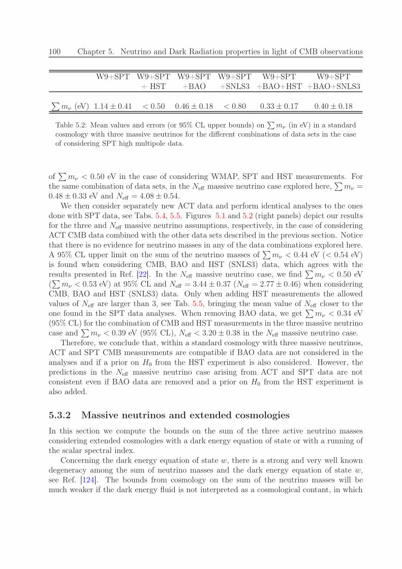
100 Chapter 5. Neutrino and Dark Radiation properties in light of CMB observations
W9+SPT W9+SPT W9+SPT W9+SPT W9+SPT W9+SPT+ HST +BAO +SNLS3 +BAO+HST +BAO+SNLS3
∑
mν (eV) 1.14 ± 0.41 < 0.50 0.46 ± 0.18 < 0.80 0.33 ± 0.17 0.40 ± 0.18
Table 5.2: Mean values and errors (or 95% CL upper bounds) on∑
mν (in eV) in a standardcosmology with three massive neutrinos for the different combinations of data sets in the caseof considering SPT high multipole data.
of∑
mν < 0.50 eV in the case of considering WMAP, SPT and HST measurements. Forthe same combination of data sets, in the Neff massive neutrino case explored here,
∑
mν =0.48 ± 0.33 eV and Neff = 4.08 ± 0.54.
We then consider separately new ACT data and perform identical analyses to the onesdone with SPT data, see Tabs. 5.4, 5.5. Figures 5.1 and 5.2 (right panels) depict our resultsfor the three and Neff massive neutrino assumptions, respectively, in the case of consideringACT CMB data combined with the other data sets described in the previous section. Noticethat there is no evidence for neutrino masses in any of the data combinations explored here.A 95% CL upper limit on the sum of the neutrino masses of
∑
mν < 0.44 eV (< 0.54 eV)is found when considering CMB, BAO and HST (SNLS3) data, which agrees with theresults presented in Ref. [22]. In the Neff massive neutrino case, we find
∑
mν < 0.50 eV(∑
mν < 0.53 eV) at 95% CL and Neff = 3.44 ± 0.37 (Neff = 2.77 ± 0.46) when consideringCMB, BAO and HST (SNLS3) data. Only when adding HST measurements the allowedvalues of Neff are larger than 3, see Tab. 5.5, bringing the mean value of Neff closer to theone found in the SPT data analyses. When removing BAO data, we get
∑
mν < 0.34 eV(95% CL) for the combination of CMB and HST measurements in the three massive neutrinocase and
∑
mν < 0.39 eV (95% CL), Neff < 3.20 ± 0.38 in the Neff massive neutrino case.Therefore, we conclude that, within a standard cosmology with three massive neutrinos,
ACT and SPT CMB measurements are compatible if BAO data are not considered in theanalyses and if a prior on H0 from the HST experiment is also considered. However, thepredictions in the Neff massive neutrino case arising from ACT and SPT data are notconsistent even if BAO data are removed and a prior on H0 from the HST experiment isalso added.
5.3.2 Massive neutrinos and extended cosmologies
In this section we compute the bounds on the sum of the three active neutrino massesconsidering extended cosmologies with a dark energy equation of state or with a running ofthe scalar spectral index.
Concerning the dark energy equation of state w, there is a strong and very well knowndegeneracy among the sum of neutrino masses and the dark energy equation of state w,see Ref. [124]. The bounds from cosmology on the sum of the neutrino masses will bemuch weaker if the dark energy fluid is not interpreted as a cosmological contant, in which
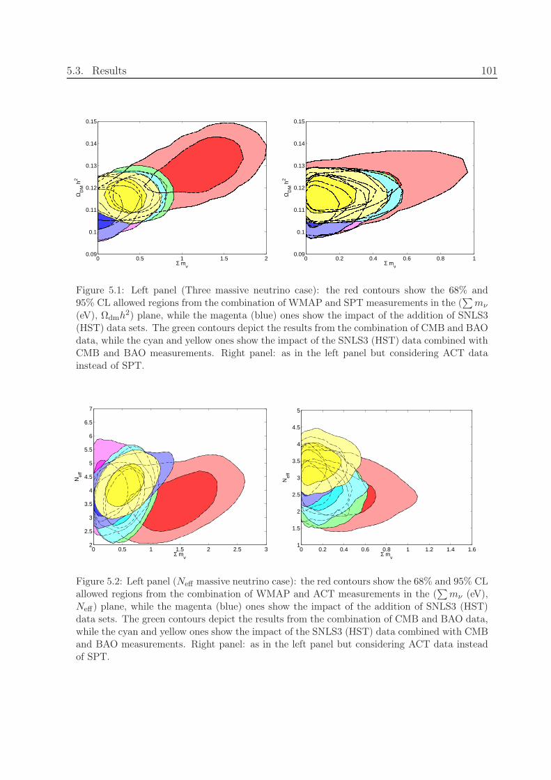
5.3. Results 101
Σ mν
ΩD
M h
2
0 0.5 1 1.5 20.09
0.1
0.11
0.12
0.13
0.14
0.15
Σ mν
ΩD
M h
2
0 0.2 0.4 0.6 0.8 10.09
0.1
0.11
0.12
0.13
0.14
0.15
Figure 5.1: Left panel (Three massive neutrino case): the red contours show the 68% and95% CL allowed regions from the combination of WMAP and SPT measurements in the (
∑
mν
(eV), Ωdmh2) plane, while the magenta (blue) ones show the impact of the addition of SNLS3(HST) data sets. The green contours depict the results from the combination of CMB and BAOdata, while the cyan and yellow ones show the impact of the SNLS3 (HST) data combined withCMB and BAO measurements. Right panel: as in the left panel but considering ACT datainstead of SPT.
Σ mν
Nef
f
0 0.5 1 1.5 2 2.5 32
2.5
3
3.5
4
4.5
5
5.5
6
6.5
7
Σ mν
Nef
f
0 0.2 0.4 0.6 0.8 1 1.2 1.4 1.61
1.5
2
2.5
3
3.5
4
4.5
5
Figure 5.2: Left panel (Neff massive neutrino case): the red contours show the 68% and 95% CLallowed regions from the combination of WMAP and ACT measurements in the (
∑
mν (eV),Neff) plane, while the magenta (blue) ones show the impact of the addition of SNLS3 (HST)data sets. The green contours depict the results from the combination of CMB and BAO data,while the cyan and yellow ones show the impact of the SNLS3 (HST) data combined with CMBand BAO measurements. Right panel: as in the left panel but considering ACT data insteadof SPT.

102 Chapter 5. Neutrino and Dark Radiation properties in light of CMB observations
W9+SPT W9+SPT W9+SPT W9+SPT W9+SPT W9+SPT+ HST +BAO +SNLS3 +BAO+HST +BAO+SNLS3
Neff 3.66 ± 0.61 4.08 ± 0.54 3.76 ± 0.67 4.04 ± 0.68 4.21 ± 0.46 3.87 ± 0.68
∑
mν (eV) 1.35 ± 0.55 0.48 ± 0.33 0.56 ± 0.22 < 0.91 0.56 ± 0.23 0.50 ± 0.21
Table 5.3: Mean values and errors(or 95% CL bounds) on Neff and∑
mν (in eV) in a standardcosmology with Neff massive neutrinos for the different combinations of data sets in the caseof considering SPT high multipole data.
W9+ACT W9+ACT W9+ACT W9+ACT W9+ACT W9+ACT+ HST +BAO +SNLS3 +BAO+HST +BAO+SNLS3
∑
mν (eV) < 0.89 < 0.34 < 0.53 < 0.49 < 0.44 < 0.54
Table 5.4: 95% CL upper bounds on∑
mν (in eV) in a standard cosmology with three massiveneutrinos for the different combinations of data sets in the case of considering ACT highmultipole data.
W9+ACT W9+ACT W9+ACT W9+ACT W9+ACT W9+ACT+ HST +BAO +SNLS3 +BAO+HST +BAO+SNLS3
Neff 2.64 ± 0.51 3.20 ± 0.38 2.63 ± 0.48 2.75 ± 0.44 3.44 ± 037 2.78 ± 0.46
∑
mν (eV) < 0.95 < 0.39 < 0.55 < 0.44 < 0.50 < 0.53
Table 5.5: Mean values and errors on Neff and 95% CL upper bounds on∑
mν (in eV) in astandard cosmology with Neff massive neutrinos for the different combinations of data sets inthe case of considering ACT high multipole data.

5.3. Results 103
case, the dark energy equation of state will be an extra free parameter. If w is allowed tovary, Ωdm can be much higher and consequently the neutrino mass also increases to leaveunchanged the matter power spectrum and the growth of matter perturbations. The SPTcollaboration [20] has also considered the impact of a constant dark energy equation of statew, and they find
∑
mν = 0.27 ± 0.11 eV for the combination of their CMB and clustersdata with WMAP 7 year, HST and BAO data sets. Figure 5.3, left panel, shows our resultsfor SPT data within the different combinations of data sets addressed here. Notice that, ingeneral, the evidence for neutrino masses in much milder than in the cosmological constantcase, and the bounds on
∑
mν are much larger than those shown in Tab. 5.2 due to thedegeneracy between
∑
mν and w. Supernovae measurements are, for this particular case,more useful than the H0 prior from the HST experiment. Figure 5.3, right panel, showsthe constraints in the (
∑
mν (eV), w) plane in the case of considering ACT data. Noticethat the bounds on
∑
mν are tighter than those found for the case of analysing SPT data.Indeed, the bounds on the sum of the three massive neutrino masses computed for the caseof a dark energy equation of state w 6= −1 are not very different from those obtained for aΛCDM universe, see Tab. 5.4. SNLS3 measurements have a much larger constraining powerthan the HST prior also in the ACT data analyses performed in this section, especially formeasuring the dark energy equation of state w.
We also explore the case in which a running in the spectral index of primordial pertur-bations is added to the minimal ΛCDM cosmology. In general, the spectrum of the scalarperturbations is not exactly a power law but it varies with scale. Therefore one must con-sider the scale dependent running of the spectral index nrun = dns/d ln k. Following [207],the power spectrum for the scalar perturbations reads
P (k) ≡ Askn(k) ∝
(
k
k0
)ns +ln(k/k0)(dn/d ln k)+ ···
,
being k0 = 0.002 Mpc−1 the pivot scale. Figure 5.4, left panel, shows our results for SPTdata within the different combinations of data sets addressed here. The evidence for neutrinomasses found for the SPT data in the cosmological constant case disappears in all the datacombinations explored here. We find, for the case of the SPT data analyses, a 2σ preferencefor a negative running, in agreement with the results presented in Ref. [20].
Figure 5.4, right panel, shows our results for ACT data in the case of considering arunning in the scalar spectral index. The bounds on the sum of the three massive neutrinosare now very similar to those found for the SPT experiment and also very similar to thosefound for ACT in the case of the minimal ΛCDM scenario. However, the preferred regionfor nrun is perfectly consistent with no running of the scalar spectral index, in agreementwith the results presented by the ACT team [22].
5.3.3 Standard cosmology plus dark radiation
In this section we explore the bounds on the Neff parameter, neglecting light neutrino massesand therefore assuming that there exist in nature Neff massless neutrino species. The left(right) panel of Fig. 5.5 shows the constraints in the (Ωdmh
2, Neff) plane arising from the
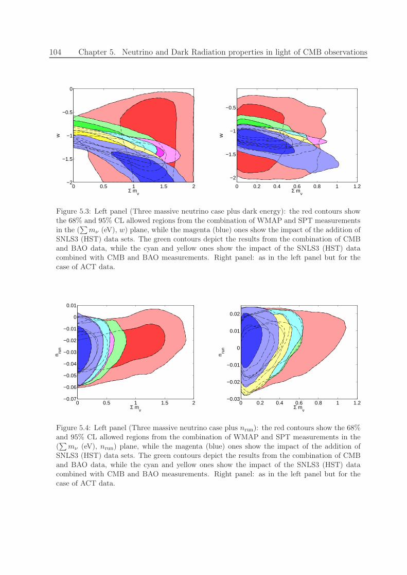
104 Chapter 5. Neutrino and Dark Radiation properties in light of CMB observations
Σ mν
w
0 0.5 1 1.5 2−2
−1.5
−1
−0.5
0
Σ mν
w
0 0.2 0.4 0.6 0.8 1 1.2
−2
−1.5
−1
−0.5
Figure 5.3: Left panel (Three massive neutrino case plus dark energy): the red contours showthe 68% and 95% CL allowed regions from the combination of WMAP and SPT measurementsin the (
∑
mν (eV), w) plane, while the magenta (blue) ones show the impact of the addition ofSNLS3 (HST) data sets. The green contours depict the results from the combination of CMBand BAO data, while the cyan and yellow ones show the impact of the SNLS3 (HST) datacombined with CMB and BAO measurements. Right panel: as in the left panel but for thecase of ACT data.
Σ mν
n run
0 0.5 1 1.5 2−0.07
−0.06
−0.05
−0.04
−0.03
−0.02
−0.01
0
0.01
Σ mν
n run
0 0.2 0.4 0.6 0.8 1 1.2−0.03
−0.02
−0.01
0
0.01
0.02
Figure 5.4: Left panel (Three massive neutrino case plus nrun): the red contours show the 68%and 95% CL allowed regions from the combination of WMAP and SPT measurements in the(∑
mν (eV), nrun) plane, while the magenta (blue) ones show the impact of the addition ofSNLS3 (HST) data sets. The green contours depict the results from the combination of CMBand BAO data, while the cyan and yellow ones show the impact of the SNLS3 (HST) datacombined with CMB and BAO measurements. Right panel: as in the left panel but for thecase of ACT data.

5.3. Results 105
ΩDM
h2
Nef
f
0.08 0.1 0.12 0.14 0.161
1.5
2
2.5
3
3.5
4
4.5
5
5.5
6
ΩDM
h2
Nef
f
0.08 0.1 0.12 0.14 0.161
1.5
2
2.5
3
3.5
4
4.5
5
5.5
6
Figure 5.5: Left panel (Massless neutrino case): the red contours show the 68% and 95% CLallowed regions from the combination of WMAP and SPT measurements in the (Ωdmh2, Neff)plane, while the magenta (blue) ones show the impact of the addition of SNLS3 (HST) datasets. The green contours depict the results from the combination of CMB and BAO data, whilethe cyan and yellow ones show the impact of the SNLS3 (HST) data combined with CMB andBAO measurements. Right panel: as in the left panel but considering ACT data instead ofSPT CMB data.
combination of WMAP plus SPT (ACT) as well as the other data combinations shown inthe previous sections. Notice that the mean value of Neff is, in general, much higher inthe case of the SPT data analyses. When considering CMB data only, Neff = 3.93 ± 0.68for the case of WMAP plus SPT data, while Neff = 2.74 ± 0.47 if analysing WMAP andACT data. The tension among these two Neff mean values gets diluted if BAO data anda prior on H0 from the HST experiment are added in the analyses. In that case, Neff =3.83±0.41 (Neff = 3.43±0.36) for WMAP plus SPT (ACT), being these two measurementsperfectly consistent and indicating both Neff > 3 at 1-2 standard deviations. The additionof SNLS3 data will not help much in improving the agreement between these two data sets,see Tabs. 5.6 and 5.7, where we summarise the mean values and errors found for Neff forthe different data combinations considered here. Therefore, as in the three massive neutrinocase, the consistency between ACT and SPT CMB results is greatly improved if BAO andHST data are considered as well.
5.3.4 Massive neutrinos and dark radiation
In this section we consider extended dark radiation cosmologies, parameterised via the darkradiation abundance Neff and its clustering properties, represented by c2eff and c2vis, see alsoRefs. [198, 199, 200] for bounds on these parameters within different cosmological models.Here three possible scenarios are examined. In the first scenario there are three massiveneutrinos with
∑
mν = 0.3 eV, which roughly corresponds to the mean value obtained inRef. [20], and ∆Neff massless neutrino species with c2vis = c2eff = 1/3. In the second scenario

106 Chapter 5. Neutrino and Dark Radiation properties in light of CMB observations
W9+SPT W9+SPT W9+SPT W9+SPT W9+SPT W9+SPT+ HST +BAO +SNLS3 +BAO+HST +BAO+SNLS3
Neff 3.93 ± 0.68 3.59 ± 0.39 3.50 ± 0.59 3.96 ± 0.69 3.83 ± 0.41 3.55 ± 0.63
Table 5.6: Mean values and errors on Neff in a standard cosmology with Neff massless neutrinosfor the different combinations of data sets in the case of considering high multipole data fromSPT.
W9+ACT W9+ACT W9+ACT W9+ACT W9+ACT W9+ACT+ HST +BAO +SNLS3 +BAO+HST +BAO+SNLS3
Neff 2.74 ± 0.47 3.12 ± 0.38 2.77 ± 0.49 2.79 ± 0.47 3.43 ± 0.36 2.83 ± 0.47
Table 5.7: Mean values and errors on Neff in a standard cosmology with Neff massless neutrinosfor the different combinations of data sets in the case of considering high multipole data fromACT.
the clustering parameters of the dark radiation component are allowed to vary, as well as inthe third scenario, in which also the sum pf the masses of the three massive neutrinos
∑
mν
varies. Our findings are summarised in Figs. 5.7 and 5.6, where we illustrate the constraintsfrom SPT and ACT probes.
In the first scenario, in which both c2eff and c2vis are fixed to their standard values andassuming three massive neutrinos with
∑
mν = 0.3 eV, we find that ∆Neff = 0.89 ± 0.56(∆Neff = 0.42 ± 0.34) when considering WMAP plus SPT (ACT) measurements. WhenHST data are added in the analyses, the mean values of ∆Neff for these two probes aresimilar: ∆Neff = 0.95 ± 0.42 (∆Neff = 0.71 ± 0.40) for WMAP, SPT and HST (WMAP,ACT and HST) measurements. The addition of BAO data does not improve the agreementbetween SPT and ACT.
In the second scenario, only∑
mν = 0.3 eV remains as a fixed parameter. In thiscase, the discrepancy between SPT and ACT data sets is larger, being the mean values for∆Neff = 1.31±0.60 and ∆Neff = 0.38±0.32 respectively. The addition of HST brings thesetwo mean values closer, being ∆Neff = 0.92±0.39 (∆Neff = 0.62±0.41) for the combinationsof WMAP, SPT and HST (WMAP, ACT and HST) data sets. Concerning the values ofthe dark radiation clustering parameters c2eff and c2vis, we find that SPT data exclude thestandard value of c2vis = 1/3 at the 2σ CL. The mean value is c2vis = 0.15 ± 0.07 (c2vis < 0.28at 95% CL) when combining SPT, WMAP, BAO and HST data sets. The results for theeffective speed of sound seem to be consistent with standard expectations, finding, for thesame combination of data sets, that c2eff = 0.32 ± 0.012. Similar results are obtained when
5.4. Conclusions 107
SPT data is combined with the other data sets considered here. However, the results of theanalyses of ACT data provide values for the clustering parameters which perfectly agreewith standard expectations, being c2eff = 0.35 ± 0.02 and c2vis = 0.25 ± 0.13 (c2vis < 0.61 at95% CL) for the analysis of ACT, WMAP, BAO and HST data sets.
In the third scenario, all four parameters ∆Neff , c2vis, c2eff and
∑
mν are allowed to freelyvary, and we depict the constraints arising from our analyses in Figs. 5.6. The evidence forneutrino masses when analysing SPT data gets diluted for all the data combinations exceptwhen BAO data is also added in the analyses. We find ∆Neff = 1.34 ± 0.67, (∆Neff =1.15 ± 0.64) and
∑
mν < 1.3 eV (∑
mν < 1.75 eV) at 95% CL when considering CMB(CMB plus HST) measurements. For the combination of WMAP, SPT and BAO (WMAP,SPT, BAO and HST) data sets, the cosmological evidence for neutrino masses still remains,finding that ∆Neff = 1.30±0.77 (∆Neff = 1.35±0.50) and
∑
mν = 0.68±0.31 eV (∑
mν =0.67 ± 0.29 eV). When analysing ACT data (see right panel of Fig. 5.6) the bounds onboth ∆Neff and
∑
mν are tighter than those found for SPT data. For the combinationof WMAP, ACT, HST and BAO data sets, ∆Neff = 0.74 ± 0.40 and
∑
mν < 0.46 eV at95% CL. Regarding the values of c2eff and c2vis, we find very similar results to those shownpreviously. In this third scenario in which the sum of the three massive neutrinos is also a freeparameter, we find that SPT data again exclude the standard value of c2vis = 1/3 at the 2σCL, while the value of c2eff agrees with its standard prediction. The analysis of SPT, WMAP,BAO and HST gives c2vis = 0.13±0.07 (c2vis < 0.26 at 95% CL) and c2eff = 0.32±0.01. In thecase of ACT data, the values for both clustering parameters perfectly agree with standardexpectations, being c2eff = 0.35± 0.02 and c2vis = 0.25± 0.11 (c2vis < 0.47 at 95% CL) for theanalysis of ACT, WMAP, BAO and HST data sets.
Figure 5.7, left (right) panel, shows the constraints on the dark radiation abundanceversus the effective speed of sound (viscosity parameter) for the combination of SPT orACT with WMAP, BAO and HST measurements. Note that SPT and ACT data seem tobe again in disagreement, this time concerning the dark radiation clustering parameter c2vis.
5.4 Conclusions
New Cosmic Microwave Background measurements have become recently available, moti-vating us to explore the improvements in the measurements of the properties of the cosmicneutrino and dark radiation backgrounds. Interestingly, the new measurements of the CMBdamping tail from the South Pole Telescope, SPT, and from the Atacama Cosmology Tele-scope, ACT, seem to give different results concerning neutrino masses and abundances.While the SPT collaboration finds ∼ 3σ evidence for neutrino masses and Neff > 3 at ∼ 2σ,the ACT collaboration does not find evidence for neutrino masses and their value for Neff
is much lower, agreeing perfectly with the standard model prediction of Neff = 3. Thesuccess of future Majorana neutrino searches relies on the absolute scale of neutrino masses;therefore a detailed analysis of both data sets separately combined with other cosmologicalmeasurements is mandatory. We have considered the most recent Baryon Acoustic Oscilla-tion data, measurements of the Hubble constant from the Hubble Space Telescope, as well
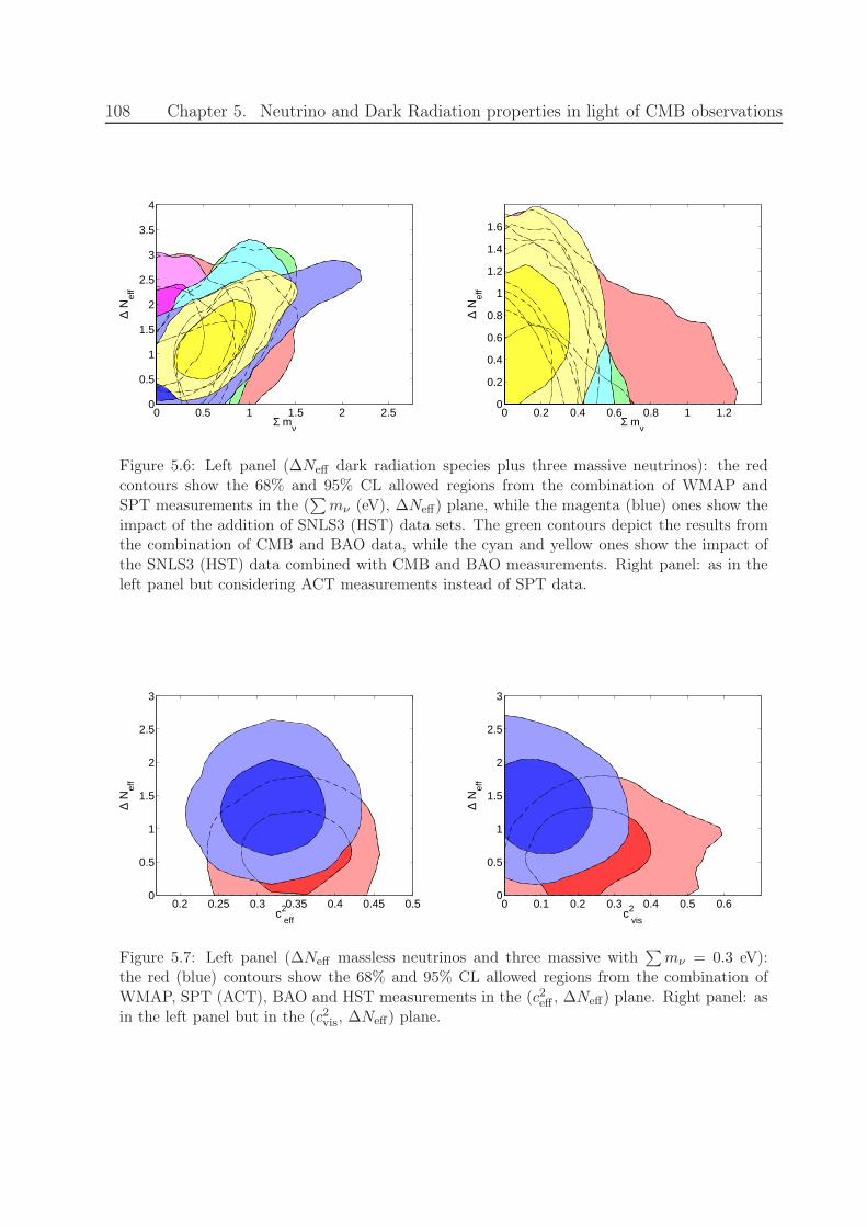
108 Chapter 5. Neutrino and Dark Radiation properties in light of CMB observations
Σ mν
∆ N
eff
0 0.5 1 1.5 2 2.50
0.5
1
1.5
2
2.5
3
3.5
4
Σ mν
∆ N
eff
0 0.2 0.4 0.6 0.8 1 1.20
0.2
0.4
0.6
0.8
1
1.2
1.4
1.6
Figure 5.6: Left panel (∆Neff dark radiation species plus three massive neutrinos): the redcontours show the 68% and 95% CL allowed regions from the combination of WMAP andSPT measurements in the (
∑
mν (eV), ∆Neff) plane, while the magenta (blue) ones show theimpact of the addition of SNLS3 (HST) data sets. The green contours depict the results fromthe combination of CMB and BAO data, while the cyan and yellow ones show the impact ofthe SNLS3 (HST) data combined with CMB and BAO measurements. Right panel: as in theleft panel but considering ACT measurements instead of SPT data.
c eff2
∆ N
eff
0.2 0.25 0.3 0.35 0.4 0.45 0.50
0.5
1
1.5
2
2.5
3
c vis2
∆ N
eff
0 0.1 0.2 0.3 0.4 0.5 0.60
0.5
1
1.5
2
2.5
3
Figure 5.7: Left panel (∆Neff massless neutrinos and three massive with∑
mν = 0.3 eV):the red (blue) contours show the 68% and 95% CL allowed regions from the combination ofWMAP, SPT (ACT), BAO and HST measurements in the (c2
eff , ∆Neff) plane. Right panel: asin the left panel but in the (c2
vis, ∆Neff) plane.
5.4. Conclusions 109
as Supernovae Ia luminosity distance measurements. In the standard ΛCDM scenario witheither three massive neutrino species or Neff massless species, the results from the two highCMB multiple probes are consistent if Baryon Acoustic Oscillation data is removed fromthe analyses and a prior on H0 from HST is also considered. In the case of Neff massiveneutrino species, SPT and ACT data analyses give very different results for
∑
mν : whilethe evidence for
∑
mν ∼ 0.5 eV found for SPT data persists independently of the data setscombined, the ACT data provide a 95% CL upper bound of ∼ 0.4 eV on
∑
mν . We thenexplore extended cosmologies models, finding that, in general, the SPT data evidence forneutrino masses found in the minimal ΛCDM scenario gets diluted except for the case of adark radiation background of unknown clustering properties with BAO data included. Inthe former case, SPT data exclude the standard value for the viscosity parameter of the darkradiation fluid c2vis = 1/3 at the 2σ CL, regardless of the data sets considered in the analysis.Upcoming, high precision CMB data from the Planck satellite will help in disentangling thehigh tail CMB neutrino–dark radiation puzzle.

110 Chapter 5. Neutrino and Dark Radiation properties in light of CMB observations
Chapter 6
Dark Radiation and interacting scenarios
In this Chapter we derive the cosmological constraints on the dark radiation abundance, onits effective velocity and on its viscosity parameter from current data in dark radiation-darkmatter coupled models. This Chapter is a copy of the paper:
Dark Radiation and interacting scenarios, Roberta Diamanti, Elena Giusarma, OlgaMena, Maria Archidiacono & Alessandro Melchiorri, 2013, Physical Review D 87, 063509.
6.1 Introduction
From observations of the Cosmic Microwave Background (CMB) and large scale structure(LSS) we can probe the fundamental properties of the constituents of the cosmic darkradiation background. The energy density of the total radiation component reads
ρrad =
[
1 +7
8
(
4
11
)4/3
Neff
]
ργ , (6.1)
where ργ is the current energy density of the CMB andNeff is a free parameter, defined as theeffective number of relativistic degrees of freedom in the cosmic dark radiation background.In the standard scenario, the expected value is Neff = 3.046, corresponding to the threeactive neutrino contribution and considering effects related to non-instantaneous neutrinodecoupling and QED finite temperature corrections to the plasma. The most recent CMBdata analyses gives Neff = 3.89± 0.67 (68% CL) [18], see also Refs. [196, 93, 94, 91, 90, 208,92, 87, 19, 209, 210, 200, 190, 191, 211, 199, 212]. The simplest scenario to explain the extradark radiation ∆Neff ≡ Neff − 3.046 arising from cosmological data analyses assumes theexistence of extra sterile neutrino species. However, there are other possibilities which areas well closely related to minimal extensions to the standard model of elementary particles,as axions, extra dimensions or asymmetric dark matter models.
Dark radiation, apart from being parametrized by its effective number of relativisticdegrees of freedom, Neff , is also characterized by its clustering properties, i.e, its rest-framespeed of sound, c2eff , and its viscosity parameter, c2vis, which controls the relationship betweenvelocity/metric shear and anisotropic stress in the dark radiation background [79]. A value
111
112 Chapter 6. Dark Radiation and interacting scenarios
of c2vis different from zero, as expected in the standard scenario, sustains the existenceof dark radiation anisotropies [213]. The standard value of c2vis = 1/3 implies that theanisotropies in the dark radiation background are present and they are identical to theneutrino viscosity. On the other hand, the case c2vis = 0 cuts the Boltzmann hierarchyof the dark radiation perturbations at the quadrupole, representing a perfect fluid withdensity and velocity (pressure) perturbations exclusively. A value of c2eff different fromthe canonical c2eff = 1/3 leads to a non-adiabatic dark radiation pressure perturbation, i.e.(δp − δρ/3)/ρ = (c2eff − 1/3)δrest
dr , where δrestdr is the density perturbation in the rest frame,
where the dark radiation velocity perturbation is zero.Interacting dark radiation arises naturally in the so-called asymmetric dark matter mod-
els (see e.g. [80] and references therein), in which the dark matter production mechanismis similar and related to the one in the baryonic sector. In these models, there exists aparticle-antiparticle asymmetry at high temperatures in the dark matter sector. The ther-mally symmetric dark matter component will annihilate and decay into dark radiation de-grees of freedom. Since the dark radiation and the dark matter fluids are interacting, therewas an epoch in the early Universe in which these two dark fluids were strongly coupled.This results in a tightly coupled fluid with a pressure producing oscillations in the matterpower spectrum analogous to the acoustic oscillations in the baryon-photon fluid beforethe recombination era. Due to the presence of a dark radiation-dark matter interaction, theclustering properties of the dark radiation component can be modified [209]. In other words,if dark radiation is made of interacting particles, the values of the clustering parameters c2effand c2vis may differ from the canonical c2eff = c2vis = 1/3.
The cosmological implications of interacting dark radiation with canonical clusteringproperties have been carefully explored in Refs. [81, 214, 78], see also the recent work ofRef. [212]. Here we generalize the analysis and leave the three dark radiation parameters∆Neff , c2eff and c2vis to vary freely within a ΛCDM scenario with a dark radiation-darkmatter interaction. We will see that the bounds from current cosmological data on the darkradiation properties derived in non interacting schemes in Refs. [200, 209, 199] will be, ingeneral, relaxed, when an interaction between the dark radiation and the dark matter fluidsis switched on. While the bounds on the number of extra dark radiation species will not belargely modified in coupled schemes, the errors on the dark radiation effective velocity andviscosity parameters will be drastically increased in interacting scenarios. We also show herehow future CMB measurements, as those from the Planck [215] and COrE [216] experiments,can lead to large biases on the dark radiation clustering parameters if the dark radiationand dark matter fluids interact in nature but the data is analyzed in the absence of such acoupling.
The paper is organized as follows. Section 6.2 presents the parametrization used fordark radiation, describing the dark radiation-dark matter interactions explored here andtheir impact on the cosmological observables used in the analysis, as the CMB temperatureanisotropies and the matter power spectrum. In Sec. 6.3 we describe the data sets usedin the Monte Carlo analyses presented in Sec. 6.4, which summarizes the constraints oninteracting dark radiation properties from current cosmological data. Future CMB darkradiation measurements are presented in Sec. 6.5. We draw our conclusions in Sec. 6.6.
6.2. Dark radiation-dark matter interaction model 113
6.2 Dark radiation-dark matter interaction model
The evolution of the dark radiation linear perturbations reads [79]
δdr −a
a(1 − 3c2eff)
(
δdr + 4a
a
θdr
k2
)
+4
3θdr +
2
3h = 0 ; (6.2)
θdr − 3k2c2eff
(
1
4δdr +
a
a
θdr
k2
)
+a
aθdr +
1
2k2πdr = 0 ; (6.3)
πdr +3
5kFdr,3 −
8
5c2vis
(
θdr
k+ σ
)
= 0 ; (6.4)
2l + 1
kFdr,3 − lFdr,l−1 + (l + 1)Fdr,l+1 = 0 l ≥ 3 , (6.5)
where the dots refer to derivatives with respect to conformal time, a is the scale factor, kis the wavenumber, c2eff is the effective sound speed, c2vis is the viscosity parameter, δdr andθdr are the dark radiation energy density perturbation and velocity divergence, respectively,and Fdr,l are the higher order moments of the dark radiation distribution function. Inthe set of equations above, πdr is the anisotropic stress perturbation, and σ is the metricshear, defined as σ = (h + 6η)/(2k), with h and η the scalar metric perturbations in thesynchronous gauge. The anisotropic stress would affect the density perturbations, as inthe case of a real fluid, in which the stress represents the viscosity, damping the densityperturbations. The relationship between the metric shear and the anisotropic stress can beparametrized through a “viscosity parameter”, c2vis [79]:
π = −3a
aπ + 4c2vis (θ + σ) , (6.6)
where θ is the divergence of the fluid velocity. Although the perturbed Einstein and energy-momentum conservation equations are enough to describe the evolution of the cosmologicalperturbations of non-relativistic particles, it is convenient to introduce the full distributionfunction in phase space to follow the perturbation evolution of relativistic particles, thatis, to consider their Boltzmann equation. In order to determine the evolution equation ofdark radiation, the Boltzmann equation is transformed into an infinite hierarchy of momentequations, that must be truncated at some maximum multipole order ℓmax. Then, thehigher order moments of the distribution function are truncated with appropriate boundaryconditions, following Ref. [82].
In the presence of a dark radiation-dark matter interaction, the Euler equations for thesetwo dark fluids read
θdm = − aaθdm +
4ρdr
3ρdmandmσdm−dr(θdr − θdm) , (6.7)
θdr =1
4k2 (δdr − 2πdr) + andmσdm−dr(θdm − θdr) (6.8)
114 Chapter 6. Dark Radiation and interacting scenarios
where the momentum transfer to the dark radiation component is given by andmσdm−dr(θdm−θdr). Indeed, the former quantity is the differential opacity, which gives the scattering rateof dark radiation by dark matter [81, 214]. The complete Euler equation for dark radiation,including the interaction term with the dark matter fluid, reads
θdr = 3k2c2eff
(
1
4δdr +
a
a
θdr
k2
)
− a
aθdr −
1
2k2πdr
+ andmσdm−dr(θdm − θdr) . (6.9)
Following Refs. [81, 214] we parameterize the coupling between massless neutrinos and darkmatter through a cross section given by
〈σdm−dr|v|〉 ∼ Q0 mdm , (6.10)
if it is constant, or
〈σdm−dr|v|〉 ∼Q2
a2mdm , (6.11)
if it is proportional to T 2, where the parameters Q0 and Q2 are constants in cm2 MeV−1
units. It has been shown in Ref. [78] that the cosmological implications of both constantand T-dependent interacting cross sections are very similar. Therefore, in the following, wefocus on the constant cross section case, parameterized via Q0.
Figure 6.1, upper panel, shows the CMB temperature anisotropies for Q0 = 10−32
cm2 MeV−1 and one dark radiation interacting species, i.e. ∆Neff = 1, as well as for thenon interacting case for the best fit parameter values from WMAP seven year data analy-sis [90, 104] together with WMAP and South Pole Telescope (SPT) data [19]. We illustratethe behavior of the temperature anisotropies for different assumptions of the dark radiationclustering parameters. Notice that the presence of a dark radiation-dark matter interactionenhances the height of the CMB peaks due to both the presence of an extra radiation com-ponent (∆Neff) and the fact that dark matter is no longer pressureless (due to a non zeroQ0). Therefore ∆Neff and Q0 will be negatively correlated. The location of the peaks alsochanges, mostly due to the presence of extra radiation ∆Neff . The peaks will be shifted tohigher multipoles ℓ due to changes in the acoustic scale, given by
θA =rs(zrec)
rθ(zrec), (6.12)
where rθ(zrec) and rs(zrec) are the comoving angular diameter distance to the last scatteringsurface and the sound horizon at the recombination epoch zrec, respectively. Althoughrθ(zrec) almost remains the same for different values of ∆Neff , rs(zrec) becomes smallerwhen ∆Neff is increased. Therefore, the positions of the acoustic peaks are shifted to highermultipoles (smaller angular scales) if the value of ∆Neff is increased. Notice, however,that this effect can be compensated by changing the cold dark matter density, in such away that zrec remains fixed, see Ref. [87]. Changing c2vis modifies the ability of the darkradiation to free-stream out of the potential wells [217, 218, 219]. Notice from Fig. 6.1
6.2. Dark radiation-dark matter interaction model 115
(upper panel), that lowering c2vis to the value c2vis = 0, the TT power spectrum is enhancedwith respect to the standard case without the dark radiation and the dark matter speciesinteracting. This situation can be explained, roughly, as the dark radiation componentbecoming a perfect fluid. That is, we are dealing with a single fluid characterized by aneffective viscosity. Disregarding the fluid nature and the physical origin of the viscosity, thegeneral consideration holds: for a given perturbation induced in the fluid, the amplitudeof the oscillations that the viscosity produces (see, e.g. [209]) increases as the viscosity isreduced. Therefore, lowering c2vis diminishes the amount of damping induced by the darkradiation viscosity, and, consequently, in this case, the amplitude of the CMB oscillationswill increase, increasing in turn the amplitude of the angular power spectrum. Therefore,we expect the interaction strength size Q0 and the c2vis parameter to be positively correlated.
On the other hand, a change of c2eff implies a decrease of pressure perturbations for thedark radiation component in its rest frame. As shown in Fig. 6.1 (upper panel), a decreasein c2eff from its canonical 1/3 to the value c2eff = 0 leads to a damping of the CMB peaks,since dark radiation is behaving as a pressureless fluid from the perturbation perspective.In the case of c2eff , we expect this parameter to be negatively correlated with Q0.
Figure 6.1 (lower panel) depicts the matter power spectrum in the presence of a darkradiation-dark matter interaction for different values of the dark radiation clustering param-eters (including the standard case with c2eff = c2vis = 1/3) for one dark radiation interactingspecies, i.e. ∆Neff = 1. We illustrate as well the case of a pure ΛCDM universe. Noticethat, since the dark matter fluid is interacting with the dark radiation component, the darkmatter component is no longer presureless, showing damped oscillations. The smaller wavemode at which the interaction between the dark fluids will leave a signature on the matterpower spectrum is roughly kf ∼ afH(af), which corresponds to the size of the universe atthe time that the dark radiation-dark matter interaction becomes ineffective [81, 214, 78],i.e. when H(af) = Γ(af ) (being H the Hubble parameter and Γ the effective dark radiation-dark matter scattering rate ρdr
ρdmndm〈σdm−dr|v|〉). For the case of constant dark radiation-dark
matter interacting cross section, the typical scale kf reads, for ∆Neff = 1:
kf ∼ 0.7
(
10−32 cm2 MeV−1
Q0
)1/2
hMpc−1 , (6.13)
Notice however from Fig. 6.1 (lower panel) that, while varying c2vis the matter powerspectrum barely changes, a change in c2eff changes dramatically the matter power spectrum,washing out any interacting signature. For instance, if c2eff = 0, dark radiation is a presure-less fluid which behaves as dark matter, inducing an enhancement of the matter fluctuations,and, consequently, the presence of a dark radiation-dark matter interaction will not modifythe matter power spectrum, see the lower panel of Fig. 6.1. Therefore, one might expecta degeneracy between the dark radiation-dark matter coupling and the dark radiation c2effparameter: the larger the interaction is, the smaller c2eff should be to compensate the sup-pression of power at scales k ∼ kf .
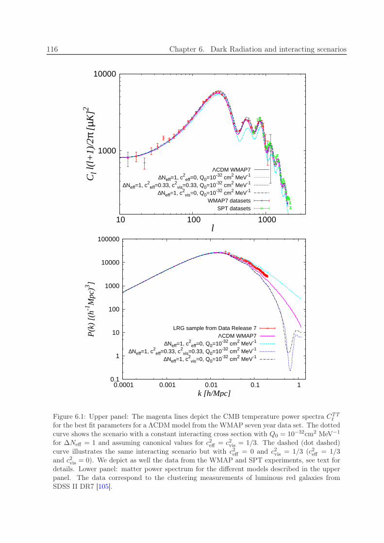
116 Chapter 6. Dark Radiation and interacting scenarios
1000
10000
10 100 1000
Cl l
(l+
1)/2
π [µ
K]2
l
ΛCDM WMAP7∆Neff=1, c2
eff=0, Q0=10-32 cm2 MeV-1
∆Neff=1, c2eff=0.33, c2
vis=0.33, Q0=10-32 cm2 MeV-1
∆Neff=1, c2vis=0, Q0=10-32 cm2 MeV-1
WMAP7 datasetsSPT datasets
0.1
1
10
100
1000
10000
100000
0.0001 0.001 0.01 0.1 1
P(k
) [(
h-1M
pc)3 ]
k [h/Mpc]
LRG sample from Data Release 7ΛCDM WMAP7
∆Neff=1, c2eff=0, Q0=10-32 cm2 MeV-1
∆Neff=1, c2eff=0.33, c2
vis=0.33, Q0=10-32 cm2 MeV-1
∆Neff=1, c2vis=0, Q0=10-32 cm2 MeV-1
Figure 6.1: Upper panel: The magenta lines depict the CMB temperature power spectra CTTℓ
for the best fit parameters for a ΛCDM model from the WMAP seven year data set. The dottedcurve shows the scenario with a constant interacting cross section with Q0 = 10−32cm2 MeV−1
for ∆Neff = 1 and assuming canonical values for c2eff = c2
vis = 1/3. The dashed (dot dashed)curve illustrates the same interacting scenario but with c2
eff = 0 and c2vis = 1/3 (c2
eff = 1/3and c2
vis = 0). We depict as well the data from the WMAP and SPT experiments, see text fordetails. Lower panel: matter power spectrum for the different models described in the upperpanel. The data correspond to the clustering measurements of luminous red galaxies fromSDSS II DR7 [105].
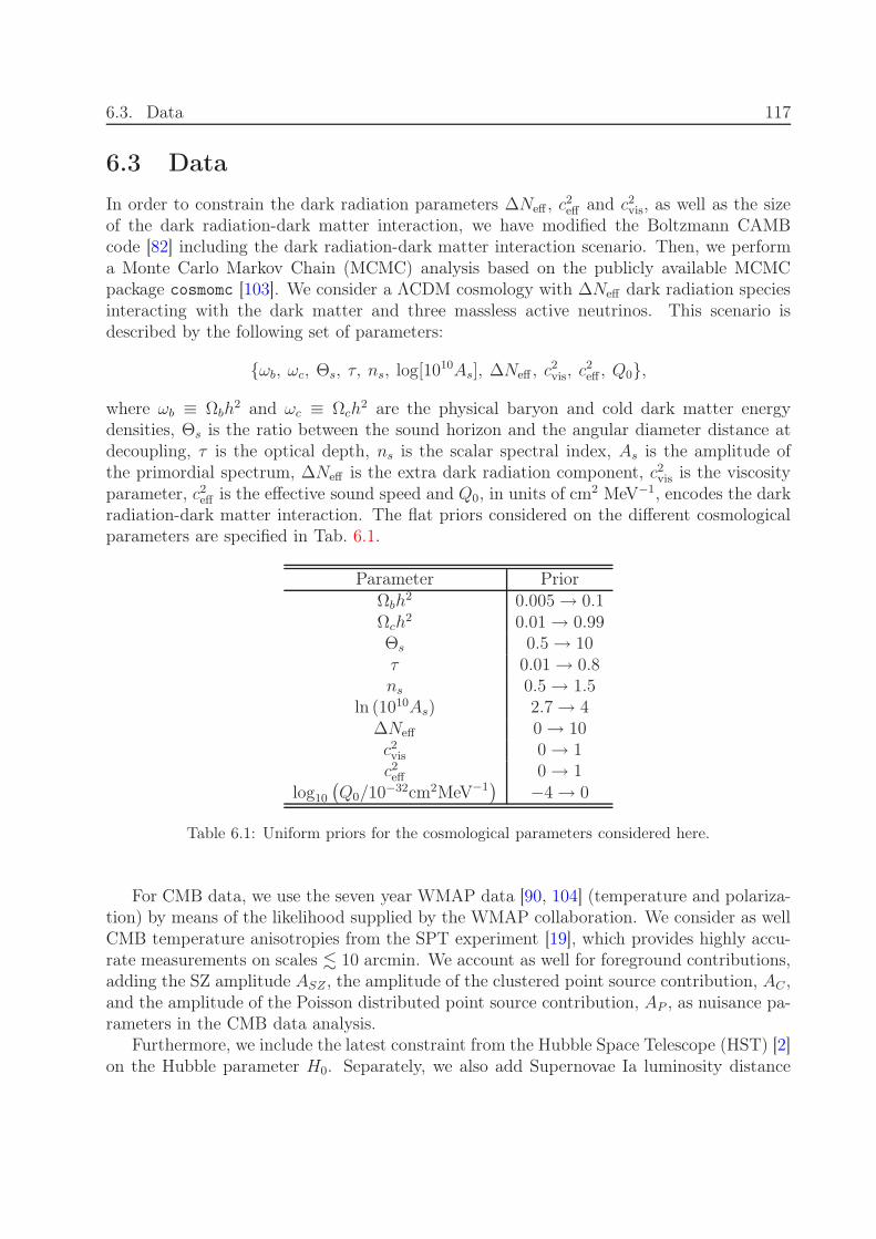
6.3. Data 117
6.3 Data
In order to constrain the dark radiation parameters ∆Neff , c2eff and c2vis, as well as the sizeof the dark radiation-dark matter interaction, we have modified the Boltzmann CAMBcode [82] including the dark radiation-dark matter interaction scenario. Then, we performa Monte Carlo Markov Chain (MCMC) analysis based on the publicly available MCMCpackage cosmomc [103]. We consider a ΛCDM cosmology with ∆Neff dark radiation speciesinteracting with the dark matter and three massless active neutrinos. This scenario isdescribed by the following set of parameters:
ωb, ωc, Θs, τ, ns, log[1010As], ∆Neff , c2vis, c
2eff , Q0,
where ωb ≡ Ωbh2 and ωc ≡ Ωch
2 are the physical baryon and cold dark matter energydensities, Θs is the ratio between the sound horizon and the angular diameter distance atdecoupling, τ is the optical depth, ns is the scalar spectral index, As is the amplitude ofthe primordial spectrum, ∆Neff is the extra dark radiation component, c2vis is the viscosityparameter, c2eff is the effective sound speed and Q0, in units of cm2 MeV−1, encodes the darkradiation-dark matter interaction. The flat priors considered on the different cosmologicalparameters are specified in Tab. 6.1.
Parameter PriorΩbh
2 0.005 → 0.1Ωch
2 0.01 → 0.99Θs 0.5 → 10τ 0.01 → 0.8ns 0.5 → 1.5
ln (1010As) 2.7 → 4∆Neff 0 → 10c2vis 0 → 1c2eff 0 → 1
log10
(
Q0/10−32cm2MeV−1)
−4 → 0
Table 6.1: Uniform priors for the cosmological parameters considered here.
For CMB data, we use the seven year WMAP data [90, 104] (temperature and polariza-tion) by means of the likelihood supplied by the WMAP collaboration. We consider as wellCMB temperature anisotropies from the SPT experiment [19], which provides highly accu-rate measurements on scales . 10 arcmin. We account as well for foreground contributions,adding the SZ amplitude ASZ , the amplitude of the clustered point source contribution, AC ,and the amplitude of the Poisson distributed point source contribution, AP , as nuisance pa-rameters in the CMB data analysis.
Furthermore, we include the latest constraint from the Hubble Space Telescope (HST) [2]on the Hubble parameter H0. Separately, we also add Supernovae Ia luminosity distance
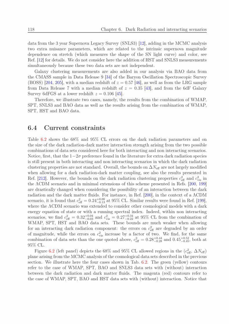
118 Chapter 6. Dark Radiation and interacting scenarios
data from the 3 year Supernova Legacy Survey (SNLS3) [12], adding in the MCMC analysistwo extra nuisance parameters, which are related to the intrinsic supernova magnitudedependence on stretch (which measures the shape of the SN light curve) and color, seeRef. [12] for details. We do not consider here the addition of HST and SNLS3 measurementssimultaneously because these two data sets are not independent.
Galaxy clustering measurements are also added in our analysis via BAO data fromthe CMASS sample in Data Release 9 [34] of the Baryon Oscillation Spectroscopic Survey(BOSS) [204, 205], with a median redshift of z = 0.57 [46], as well as from the LRG samplefrom Data Release 7 with a median redshift of z = 0.35 [43], and from the 6dF GalaxySurvey 6dFGS at a lower redshift z = 0.106 [45].
Therefore, we illustrate two cases, namely, the results from the combination of WMAP,SPT, SNLS3 and BAO data as well as the results arising from the combination of WMAP,SPT, HST and BAO data.
6.4 Current constraints
Table 6.2 shows the 68% and 95% CL errors on the dark radiation parameters and onthe size of the dark radiation-dark matter interaction strength arising from the two possiblecombinations of data sets considered here for both interacting and non interacting scenarios.Notice, first, that the 1−2σ preference found in the literature for extra dark radiation speciesis still present in both interacting and non interacting scenarios in which the dark radiationclustering properties are not standard. Overall, the bounds on ∆Neff are not largely modifiedwhen allowing for a dark radiation-dark matter coupling, see also the results presented inRef. [212]. However, the bounds on the dark radiation clustering properties c2eff and c2vis inthe ΛCDM scenario and in minimal extensions of this scheme presented in Refs. [200, 199]are drastically changed when considering the possibility of an interaction between the darkradiation and the dark matter fluids. For instance, in Ref. [200], in the context of a ΛCDMscenario, it is found that c2eff = 0.24+0.08
−0.13 at 95% CL. Similar results were found in Ref. [199],where the ΛCDM scenario was extended to consider other cosmological models with a darkenergy equation of state or with a running spectral index. Indeed, within non interactingscenarios, we find c2eff = 0.32+0.04
−0.03 and c2vis = 0.27+0.34−0.22 at 95% CL from the combination of
WMAP, SPT, HST and BAO data sets. These bounds are much weaker when allowingfor an interacting dark radiation component: the errors on c2eff are degraded by an orderof magnitude, while the errors on c2vis increase by a factor of two. We find, for the samecombination of data sets than the one quoted above, c2eff = 0.28+0.44
−0.28 and 0.45+0.52−0.45, both at
95% CL.Figure 6.2 (left panel) depicts the 68% and 95% CL allowed regions in the (c2eff , ∆Neff)
plane arising from the MCMC analysis of the cosmological data sets described in the previoussection. We illustrate here the four cases shown in Tab. 6.2. The green (yellow) contoursrefer to the case of WMAP, SPT, BAO and SNLS3 data sets with (without) interactionbetween the dark radiation and dark matter fluids. The magenta (red) contours refer tothe case of WMAP, SPT, BAO and HST data sets with (without) interaction. Notice that

6.5. Forecasts from future cosmological data 119
WMAP+SPT+ WMAP+SPT+ WMAP+SPT+ WMAP+SPT+BAO+HST int. BAO+HST no int. BAO+SNLS3 int. BAO+SNLS3 no int.
c2eff 0.28+0.10+0.44
−0.12−0.28 0.32+0.02+0.04−0.02−0.03 0.30+0.12+0.50
−0.15−0.30 0.32+0.02+0.04−0.02−0.04
c2vis 0.45+0.34+0.52
−0.31−0.45 0.27+0.13+0.34−0.13−0.22 0.46+0.36+0.51
−0.32−0.46 0.27+0.13+0.42−0.14−0.23
∆Neff 68%CL < 0.81 0.62+0.36+0.80−0.36−0.53 < 0.76 0.77+0.50+1.29
−0.72−0.72
95%CL < 1.30 < 1.47
Q0 68%CL < 0.8 — < 0.8 —(
10−33 cm2
MeV−1
)
95%CL < 4.9 — < 5.4 —
Table 6.2: 1D marginalized bounds on the dark radiation parameters and on the size of thedark radiation dark matter interaction Q0 using WMAP, SPT, BAO data and HST/SNLS3measurements, see text for details. We show the constraints for both interacting and noninteracting models, presenting the mean as well as the 68% and 95% CL errors of the posteriordistribution.
the errors on the c2eff parameter are largely increased when the interaction term is switchedon, while the errors on ∆Neff are mildly affected by the presence of such an interaction.Notice that HST data is more powerful than SNLS3 data in constraining ∆Neff , agreeingwith previous results in the literature, see Ref. [196]. The reason is because ∆Neff is highlydegenerate with H0, and HST data provide a strong prior on the former parameter.
The right panel of Fig. 6.2 depicts the 68% and 95% CL allowed regions in the (c2vis,∆Neff) plane, being the color code identical to the one used in the left panel. While theimpact of the coupling is not as large as in the effective velocity case, the errors on theviscosity parameter c2vis are enlarged by a factor of two in interacting dark radiation models.
6.5 Forecasts from future cosmological data
We evaluate here the constraints on the dark radiation parameters, ∆Neff , c2eff , c2vis, bymeans of an analysis of future mock CMB data for the ongoing Planck experiment and thefuture COrE mission. These CMB mock data sets are then fitted using a MCMC analysisto a non interacting cosmological scenario but allowing the dark radiation parameters tohave non standard values. The CMB mock data sets are generated accordingly to noiseproperties consistent with the Planck and COrE CMB missions. The fiducial Cℓ modelwe use is a ΛCDM scenario (i.e. a flat universe with a cosmological constant and threemassless active neutrino species) adding an interaction between the dark radiation and darkmatter sectors with Q0 = 10−32cm2 MeV−1, assuming one dark radiation interacting species∆Neff=1 and standard clustering and viscosity parameters for the dark radiation, i.e. c2vis =
120 Chapter 6. Dark Radiation and interacting scenarios
c2eff
∆ N
eff
0 0.2 0.4 0.6 0.8 10
0.5
1
1.5
2
2.5
c2vis
∆ N
eff
0 0.2 0.4 0.6 0.8 10
0.5
1
1.5
2
2.5
Figure 6.2: Left panel: 68% and 95% CL contours in the (c2eff , ∆Neff) plane arising from the
MCMC analysis of WMAP, SPT, BAO and HST/SNLS3 data. The green (yellow) contoursrefer to the case of WMAP, SPT, BAO and SNLS3 data sets with (without) interaction betweenthe dark radiation and dark matter fluids. The magenta (red) contours refer to the case ofWMAP, SPT, BAO and HST data sets with (without) interaction between the dark radiationand dark matter sectors. Right panel: as in the left panel but in the (c2
vis, ∆Neff) plane.
c2eff = 1/3. For each frequency channel we consider a detector noise given by ω−1 = (θσ)2,being θ the FWHM of the gaussian beam and σ = ∆T/T the temperature sensitivity (thepolarization sensitivity is ∆E/E =
√2∆T/T ). Consequently the Cℓ fiducial spectra get a
noise contribution which reads Nℓ = ω−1 exp (ℓ(ℓ+ 1)/ℓ2b), where ℓb ≡√
8ln2/θ.
Figure 6.3 (left panel) depicts the 68% and 95% CL contours in the (c2eff ,∆Neff) planearising from the MCMC analysis of Planck and COrE mock data. Notice that the recon-structed value for c2eff is larger than the simulated value c2eff = 1/3. The reason for that isdue to the degeneracy between the dark radiation-dark matter interaction Q0 and c2eff , seeFig. 6.1, from which one would expect a negative correlation between the interaction crosssection and the effective velocity. If such an interaction occurs in nature but future CMBdata is analysed assuming a non interacting model, the reconstructed value of c2eff will behigher than the standard expectation of 1/3, see Tab. 6.3. From what regards to c2vis, seeFig. 6.3 (right panel), the effect is the opposite since these two parameters are positivelycorrelated and therefore the reconstructed value of c2vis is lower than the canonical 1/3, seeTab. 6.3. Therefore, if the dark radiation and dark matter sectors interact, a large bias onthe dark radiation clustering parameters could be induced if future CMB data are analysedneglecting such coupling. On the other hand, the bias induced in ∆Neff is not very signif-icant, being the reconstructed value consistent with the ∆Neff = 1 simulated one within1σ.

6.6. Conclusions 121
c2eff
∆ N
eff
0.33 0.335 0.34 0.345 0.35 0.3550.5
1
1.5
2
2.5
c2vis
∆ N
eff
0.29 0.295 0.3 0.305 0.31 0.3150.5
1
1.5
2
2.5
Figure 6.3: Left panel: 68% and 95% CL contours in the (c2eff , ∆Neff) arising from the MCMC
analysis of Planck (red contours) and COrE (blue contours) CMB mock data. The mock dataare generated adding an interaction between the dark radiation and dark matter sectors withQ0 = 10−32cm2 MeV−1, assuming one dark radiation interacting species ∆Neff=1 and standardclustering and viscosity parameters for the dark radiation. The CMB mock data is then fittedto a non interacting cosmology but allowing the dark radiation parameters c2
eff and c2vis to have
non standard values. Right panel: as in the left panel but in the (c2vis, ∆Neff) plane.
Planck COrE
c2eff 0.35+0.003+0.005
−0.003−0.007 0.34+0.004+0.006−0.001−0.003
c2vis 0.30+0.005+0.017
−0.006−0.006 0.29+0.001+0.002−0.001−0.001
∆Neff 1.26+0.27+0.54−0.25−0.51 1.17+0.13+0.27
−0.12−0.23
Table 6.3: Constraints on the dark radiation clustering parameters from the Plank and COrEmock data sets described in the text. We present the mean as well as the 68% and 95% CLerrors of the posterior distribution. We have set Q0 = 10−32cm2 MeV−1, c2
eff = c2vis = 1/3 in
the mock data sets. Then, we have fitted these data to non interacting models in which bothc2eff and c2
vis are free parameters.
6.6 Conclusions
Standard dark radiation is made of three light active neutrinos. However, many extensionsof the standard model of elementary particles predict an extra dark radiation componentin the form of sterile neutrinos, axions or other very light degrees of freedom which mayinteract with the dark matter sector. In fact, once that one assumes the existence of extradark radiation species as well as the existence of a dark matter sector there is a priori nofundamental symmetry which forbids couplings between these two dark fluids. If one allows
122 Chapter 6. Dark Radiation and interacting scenarios
for such a possibility, the clustering properties of these extra dark radiation particles mightnot be identical to those of the standard model neutrinos, since the extra dark radiationparticles are coupled to the dark matter. In this paper we have analyzed the constraintsfrom recent cosmological data on the dark radiation abundances, effective velocities andviscosity parameters. While the bounds on ∆Neff are very close to those of uncoupledmodels, the errors on the clustering dark radiation properties are largely increased, mostlydue to the existing degeneracies among the dark radiation-dark matter coupling and c2eff ,c2vis. The cosmological bounds on the dark radiation effective velocity c2eff found in non-interacting schemes are degraded by an order of magnitude when a dark radiation-darkmatter interaction is switched on. In the case of the viscosity parameter c2vis, the errorson this parameter are a factor of two larger when considering interacting scenarios. Wehave also explored the perspectives from future Cosmic Microwave Background data. Ifdark radiation and dark matter interact in nature, but the data are analysed assuming thestandard, non interacting picture, the reconstructed values for the effective velocity andfor the viscosity parameter will be shifted from their standard 1/3 expectation, namelyc2eff = 0.34+0.006
−0.003 and c2vis = 0.29+0.002−0.001 at 95% CL for the future COrE CMB mission.

Part III
Summary and Conclusions
123

Chapter 7
Summary and Conclusions
Neutrinos are one of the most mysterious particles in nature. Nowadays we know fromexperimental results on neutrino oscillations that neutrinos are massive. Unfortunately,oscillation experiments are not sensitive to the overall neutrino mass scale.
Cosmology provides one of the means to test the absolute scale of neutrino masses andplays an important role to constrain neutrino properties. Neutrinos affect both the CosmicMicrowave Background (CMB) physics as well as the galaxy clustering, leaving a significantimprint either in the full shape clustering signal (exploited by matter power spectrum mea-surements) or in the geometrical signal (exploited via Baryon Acoustic Oscillation (BAO)measurements).
In this thesis we have derived bounds on the neutrino masses and on the neutrino abun-dances from the recent cosmological data, considering a ΛCDM scenario as well as otherextended cosmological scenarios.
Chapter I contains a brief description of the current cosmological model and the mea-surements which support it. A detailed description of the different signatures in cosmologyarising from the neutrino properties, as its mass and its abundance, can be found in ChapterII.
In Chapter III [189] we have studied a flat ΛCDM scenario with Neff active plus ster-ile massive neutrino species, in order to test the so-called (3+2) models with cosmologicaldata. We have found that this model is allowed at the 95 % CL by current cosmologicaldata (which include CMB, galaxy clustering and Supernovae Ia). We have also consideredthe Big Bang Nucleosynthesis Helium-4 and Deuterium abundances and we have foundthat these measurements compromise the viability of (3+2) models. Moreover, we havepresented a forecast to compute the errors on the active and sterile neutrino parametersfrom the ongoing Planck CMB mission data and from the BOSS and Euclid galaxy surveydata. Future cosmological data could determine sub-eV active and sterile neutrino massesand sterile neutrino abundances with 10−30% precision, for sub-eV (0.5 eV> mνs > 0.1 eV)sterile neutrino masses. We have also shown that the presence of massive sterile neutrinosin the universe could be inferred from inconsistencies among the values of the Hubble con-
125

126 Chapter 7. Summary and Conclusions
stant H0 obtained from CMB and galaxy clustering data and those arising from independentmeasurements of the Hubble constant over the next decade.
In Chapter IV [193] we have derived the neutrino mass bounds from the angular powerspectra from the BOSS experiment, part of the Sloan Digital Sky Survey III, Data ReleaseEight (BOSS DR8) photometric sample of CMASS galaxies, dividing this sample into fourphotometric redshift bins, from z = 0.45 to z = 0.65, and considering a free constant biasparameter for each of these bins. To mimic the effects of a scale dependent galaxy bias,we have also fitted the data with an additional set of shot noise-like parameters. We havecalculated the power spectra in two multipole ranges, 30 < ℓ < 150 and 30 < ℓ < 200,in order to minimize non-linear effects and we have considered a flat ΛCDM model plusthree active massive neutrino species. Combining the BOSS DR8 data with CMB WMAP7 year data, we have found an upper bound on the sum of the three active neutrino massesof∑
mν < 0.56 eV at 95% CL for ℓmax = 200 (in the model with free bias parameters)and an upper bound
∑
mν < 0.26 eV at 95% CL if a prior on the Hubble constant fromthe Hubble Space Telescope (HST) data is also included. Considering a conservative galaxybias model containing shot noise-like parameters, we have found
∑
mν < 0.90 eV at 95%CL using CMB and BOSS DR8 data and
∑
mν < 0.36 eV at 95% CL using CMB, HSTand BOSS DR8 data sets. We have also shown that the addition of Supernova and/or BAOdata does not significantly improve the neutrino mass bound once the HST prior is included.
New measurements of the CMB damping tail released in late 2012 and early 2013 fromthe South Pole Telescope, SPT, and from the Atacama Cosmology Telescope, ACT, seem togive different results concerning neutrino masses and abundances. Motivated by the discrep-ancies between SPT and ACT findings, we have explored in Chapter V [221] the cosmologicalconstraints in several neutrino and dark radiation scenarios using CMB WMAP 9 year data,the new SPT and ACT measurements at high multipoles ℓ, BAO data, HST measurementsof the Hubble constant and Supernovae Ia luminosity distance data. In the standard ΛCDMscenario with either three massive neutrino species or Neff massless species, the two high ℓCMB probes give similar results if BAO data are removed from the analyses and a prior onH0 from HST is also considered. In the case of Neff massive neutrino species, SPT and ACTdata analyses give very different results for
∑
mν : while the evidence for∑
mν ∼ 0.5 eVfound for SPT data persists independently of the data sets combined in the analysis, theACT data provide a 95% CL upper bound of ∼ 0.4 eV on
∑
mν . We then have exploredextended cosmological scenarios with a dark energy equation of state and with a running ofthe scalar spectral index and we have proved that the evidence for neutrino masses found bythe South Pole Telescope in the three neutrino scenario disappears for all the data combina-tions. Again, the agreement between the two high multipole CMB measurements consideredis highly improved when adding HST data. Finally, we have considered the case of a darkradiation background of unknown clustering properties, finding that SPT data exclude thestandard value for the viscosity parameter of the dark radiation fluid c2vis = 1/3 at the 2σ CL.
In Chapter VI [198] we have studied a dark radiation-dark matter interacting model

127
deriving the constraints from recent cosmological data on the dark radiation abundances,effective velocities and viscosity parameters. If one assumes the existence of extra dark radi-ation species interacting with the dark matter sector, the clustering properties of these extradark radiation particles might not be identical to those of the Standard Model neutrinos(for which c2eff = c2vis = 1/3), since the extra dark radiation particles are coupled to the darkmatter fluid. We have found that the cosmological bounds on the number of extra darkradiation species do not change significantly when considering interacting schemes, whilethe errors on the clustering dark radiation properties are largely increased, mostly due tothe existing degeneracies among the dark radiation-dark matter coupling and c2eff , c2vis. Thecosmological bounds on the dark radiation effective velocity c2eff found in non-interactingschemes are degraded by an order of magnitude when a dark radiation-dark matter interac-tion is switched on. In the case of the viscosity parameter c2vis, the errors on this parameterare a factor of two larger when considering interacting scenarios. We have also explored theperspectives from future CMB measurements. If dark radiation and dark matter interactin nature, but the data are analysed assuming the standard, non interacting picture, thereconstructed values for the effective velocity and for the viscosity parameter will be shiftedfrom their standard 1/3 expectation, namely c2eff = 0.34+0.006
−0.003 and c2vis = 0.29+0.002−0.001 at 95% CL
for the future COrE CMB mission.
Latest measurements of the CMB temperature anisotropies released by the Planck satel-lite provide the tightest constraints on cosmological parameters [9] but they do not providea strong bound on the sum of neutrino masses if they are not combined with external datasets. The upper limit from Planck, considering lensing, combined with low-ℓ polarizationmeasurements from WMAP-9 year data is
∑
mν < 1.1 eV at 95% CL. The addition of theHST prior on the Hubble constant improves the constraints to
∑
mν < 0.21 eV at 95% CL.Planck mesurements alone find no evidence for additional relativistic particles beyond thethree families of neutrinos in the Standard Model, while the constraint obtained combiningCMB Planck data with the HST Hubble constant measurement is Neff = 3.62 ± 0.25, dueto the strong degeneracy between H0 and Neff .
The future planned Euclid galaxy survey could provide the ideal tool to test neutrinoproperties with cosmology. Combining Euclid measurements of the custering of galaxies, ofweak lensing shear and of clusters with CMB data, the sum of neutrino masses could bemeasured with a 1 σ precision of 0.01 eV assuming a fiducial model with
∑
mν = 0.056 eV,even in the case that the dark energy equation of state varies with time [220]. The samedata combination could reach a 1σ sensitivity to Neff of 0.02, implying that the smalldeparture of 0.046 from the standard expectation of 3 (arising from non instantaneousneutrino decoupling, neutrino mixing and finite temperature corrections) could be testedwith 2σ precision [220].

128 Chapter 7. Summary and Conclusions

Part IV
Bibliography
129

Bibliography
[1] S. Dodelson, “Modern cosmology,” Amsterdam, Netherlands: Academic Pr. (2003) 440p.
[2] A. G. Riess, L. Macri, S. Casertano, H. Lampeitl, H. C. Ferguson, A. V. Filippenko,S. W. Jha and W. Li et al., Astrophys. J. 730, 119 (2011) [Erratum-ibid. 732, 129(2011)] [arXiv:1103.2976 [astro-ph.CO]].
[3] P. Coles and F. Lucchin, “Cosmology: The Origin and evolution of cosmic structure,”Chichester, UK: Wiley (2002) 492 p.
[4] Einstein A., Sitzungsber. Preuss. Akad. Wiss. phys.-math. Klasse VI, 142 (1917).
[5] A. S. Eddington, Mon. Not. Roy. Astron. Soc. 90, 668 (1930).
[6] Friedmann A., 1922, ZPhy, 10, 377.
[7] Friedmann A., 1924, ZPhy, 21, 326 .
[8] C. -P. Ma and E. Bertschinger, Astrophys. J. 455, 7 (1995) [astro-ph/9506072].
[9] P. A. R. Ade et al. [ Planck Collaboration], arXiv:1303.5076 [astro-ph.CO].
[10] S. Perlmutter et al. [Supernova Cosmology Project Collaboration], Astrophys. J. 517,565 (1999) [astro-ph/9812133].
[11] A. G. Riess et al. [Supernova Search Team Collaboration], Astron. J. 116, 1009 (1998)[astro-ph/9805201].
[12] A. Conley, J. Guy, M. Sullivan, N. Regnault, P. Astier, C. Balland, S. Basa andR. G. Carlberg et al., Astrophys. J. Suppl. 192 (2011) 1 [arXiv:1104.1443 [astro-ph.CO]].
[13] E. S. Walker, I. M. Hook, M. Sullivan, D. A. Howell, P. Astier, C. Balland, S. Basa andT. J. Bronder et al., arXiv:1008.2308 [astro-ph.CO].
[14] M. Sullivan, J. Guy, A. Conley, N. Regnault, P. Astier, C. Balland, S. Basa andR. G. Carlberg et al., Astrophys. J. 737, 102 (2011) [arXiv:1104.1444 [astro-ph.CO]].
131
132 Bibliography
[15] R. Amanullah, C. Lidman, D. Rubin, G. Aldering, P. Astier, K. Barbary, M. S. Burnsand A. Conley et al., Astrophys. J. 716, 712 (2010) [arXiv:1004.1711 [astro-ph.CO]].
[16] E. L. Wright, S. S. Meyer, C. L. Bennett, N. W. Boggess, E. S. Cheng, M. G. Hauser,A. Kogut and C. Lineweaver et al., Astrophys. J. 396, L13 (1992).
[17] J. Lesgourgues, G. Mangano, G. Miele and S. Pastor “Neutrino Cosmology,” Cambridge,UK: Cambridge University Press (2013) 378 p.
[18] G. Hinshaw, D. Larson, E. Komatsu, D. N. Spergel, C. L. Bennett, J. Dunkley,M. R. Nolta and M. Halpern et al., arXiv:1212.5226 [astro-ph.CO].
[19] R. Keisler, C. L. Reichardt, K. A. Aird, B. A. Benson, L. E. Bleem, J. E. Carlstrom,C. L. Chang and H. M. Cho et al., Astrophys. J. 743, 28 (2011) [arXiv:1105.3182[astro-ph.CO]].
[20] Z. Hou, C. L. Reichardt, K. T. Story, B. Follin, R. Keisler, K. A. Aird, B. A. Bensonand L. E. Bleem et al., arXiv:1212.6267 [astro-ph.CO].
[21] K. T. Story, C. L. Reichardt, Z. Hou, R. Keisler, K. A. Aird, B. A. Benson, L. E. Bleemand J. E. Carlstrom et al., arXiv:1210.7231 [astro-ph.CO].
[22] J. L. Sievers, R. A. Hlozek, M. R. Nolta, V. Acquaviva, G. E. Addison, P. A. R. Ade,P. Aguirre and M. Amiri et al., arXiv:1301.0824 [astro-ph.CO].
[23] S. Das, T. Louis, M. R. Nolta, G. E. Addison, E. S. Battistelli, J R. Bond, E. Calabreseand D. C. M. J. Devlin et al., arXiv:1301.1037 [astro-ph.CO].
[24] J. Silk, Astrophys. J. 151, 459 (1968).
[25] P. A. R. Ade et al. [ Planck Collaboration], arXiv:1303.5062 [astro-ph.CO].
[26] M. Tegmark, astro-ph/9511148.
[27] W. Hu and S. Dodelson, Ann. Rev. Astron. Astrophys. 40, 171 (2002) [astro-ph/0110414].
[28] A. J. S. Hamilton, Lect. Notes Phys. 665, 415 (2008) [astro-ph/0503603].
[29] A. J. S. Hamilton, Lect. Notes Phys. 665, 433 (2008) [astro-ph/0503604]. HamiltonA. J. S., 2005, astro, arXiv:astro-ph/0503604
[30] Martínez V. J., 2009, LNP, 665, 269
[31] D. H. Weinberg, M. J. Mortonson, D. J. Eisenstein, C. Hirata, A. G. Riess and E. Rozo,arXiv:1201.2434 [astro-ph.CO].
[32] D. G. York et al. [SDSS Collaboration], Astron. J. 120, 1579 (2000) [astro-ph/0006396].
Bibliography 133
[33] J. A. Frieman, B. Bassett, A. Becker, C. Choi, D. Cinabro, D. F. DeJongh, D. L. Depoyand M. Doi et al., Astron. J. 135, 338 (2008) [arXiv:0708.2749 [astro-ph]].
[34] C. P. Ahn et al. [SDSS Collaboration], Astrophys. J. Suppl. 203, 21 (2012)[arXiv:1207.7137 [astro-ph.IM]].
[35] D. J. Eisenstein et al. [SDSS Collaboration], Astron. J. 142, 72 (2011) [arXiv:1101.1529[astro-ph.IM]].
[36] A. Ross, S. Ho, A. J. Cuesta, R. Tojeiro, W. J. Percival, D. Wake, K. L. Masters andR. C. Nichol et al., Mon. Not. Roy. Astron. Soc. 417, 1350 (2011) [arXiv:1105.2320[astro-ph.CO]].
[37] M. White, M. Blanton, A. Bolton, D. Schlegel, J. Tinker, A. Berlind, L. da Costa andE. Kazin et al., Astrophys. J. 728, 126 (2011) [arXiv:1010.4915 [astro-ph.CO]].
[38] M. Tegmark et al. [SDSS Collaboration], Astrophys. J. 571, 191 (2002) [astro-ph/0107418].
[39] D. Huterer, L. Knox, R. C. Nichol and , Astrophys. J. 555, 547 (2001) [astro-ph/0011069].
[40] H. Aihara et al. [SDSS Collaboration], Astrophys. J. Suppl. 193, 29 (2011) [Erratum-ibid. 195, 26 (2011)] [arXiv:1101.1559 [astro-ph.IM]].
[41] A. J. S. Hamilton, astro-ph/9708102.
[42] N. Benitez, E. Gaztanaga, R. Miquel, F. Castander, M. Moles, M. Crocce,A. Fernandez-Soto and P. Fosalba et al., Astrophys. J. 691, 241 (2009) [arXiv:0807.0535[astro-ph]].
[43] N. Padmanabhan, X. Xu, D. J. Eisenstein, R. Scalzo, A. J. Cuesta, K. T. Mehta andE. Kazin, arXiv:1202.0090 [astro-ph.CO].
[44] C. Blake, E. Kazin, F. Beutler, T. Davis, D. Parkinson, S. Brough, M. Colless andC. Contreras et al., Mon. Not. Roy. Astron. Soc. 418, 1707 (2011) [arXiv:1108.2635[astro-ph.CO]].
[45] F. Beutler, C. Blake, M. Colless, D. H. Jones, L. Staveley-Smith, L. Campbell, Q. Parkerand W. Saunders et al., Mon. Not. Roy. Astron. Soc. 416, 3017 (2011) [arXiv:1106.3366[astro-ph.CO]].
[46] L. Anderson, E. Aubourg, S. Bailey, D. Bizyaev, M. Blanton, A. S. Bolton,J. Brinkmann and J. R. Brownstein et al., Mon. Not. Roy. Astron. Soc. 428, 1036(2013) [arXiv:1203.6594 [astro-ph.CO]].
[47] L. Anderson, E. Aubourg, S. Bailey, F. Beutler, A. S. Bolton, J. Brinkmann,J. R. Brownstein and C. -H. Chuang et al., arXiv:1303.4666 [astro-ph.CO].

134 Bibliography
[48] S. Hannestad and J. Madsen, Phys. Rev. D 52, 1764 (1995) [astro-ph/9506015].
[49] A. D. Dolgov, S. H. Hansen and D. V. Semikoz, Nucl. Phys. B 543, 269 (1999) [hep-ph/9805467].
[50] G. Mangano, G. Miele, S. Pastor and M. Peloso, Phys. Lett. B 534, 8 (2002) [astro-ph/0111408].
[51] G. Mangano, G. Miele, S. Pastor, T. Pinto, O. Pisanti and P. D. Serpico, Nucl. Phys.B 729, 221 (2005) [hep-ph/0506164].
[52] Cowan C. L., Jr., Reines F., Harrison F. B., Kruse H. W., McGuire A. D., 1956, Sci,124, 103
[53] B. Pontecorvo, Sov. Phys. JETP 7, 172 (1958) [Zh. Eksp. Teor. Fiz. 34, 247 (1957)].
[54] Z. Maki, M. Nakagawa and S. Sakata, Prog. Theor. Phys. 28, 870 (1962).
[55] M. C. Gonzalez-Garcia, M. Maltoni, J. Salvado and T. Schwetz, JHEP 1212, 123 (2012)[arXiv:1209.3023 [hep-ph]].
[56] D. V. Forero, M. Tortola and J. W. F. Valle, Phys. Rev. D 86, 073012 (2012)[arXiv:1205.4018 [hep-ph]].
[57] G. L. Fogli, E. Lisi, A. Marrone, D. Montanino, A. Palazzo and A. M. Rotunno, Phys.Rev. D 86, 013012 (2012) [arXiv:1205.5254 [hep-ph]].
[58] V. M. Lobashev, Nucl. Phys. A 719, 153 (2003).
[59] C. .Kraus, B. Bornschein, L. Bornschein, J. Bonn, B. Flatt, A. Kovalik, B. Ostrick andE. W. Otten et al., Eur. Phys. J. C 40 (2005) 447 [hep-ex/0412056].
[60] A. Osipowicz et al. [KATRIN Collaboration], hep-ex/0109033.
[61] J. J. Gomez-Cadenas, J. Martin-Albo, M. Mezzetto, F. Monrabal and M. Sorel, Riv.Nuovo Cim. 35, 29 (2012) [arXiv:1109.5515 [hep-ex]].
[62] O. Mena and S. J. Parke, Phys. Rev. D 69, 117301 (2004) [hep-ph/0312131].
[63] K. N. Abazajian, M. A. Acero, S. K. Agarwalla, A. A. Aguilar-Arevalo, C. H. Albright,S. Antusch, C. A. Arguelles and A. B. Balantekin et al., arXiv:1204.5379 [hep-ph].
[64] A. Aguilar-Arevalo et al. [LSND Collaboration], Phys. Rev. D 64, 112007 (2001) [hep-ex/0104049].
[65] A. A. Aguilar-Arevalo et al. [MiniBooNE Collaboration], Phys. Rev. Lett. 98, 231801(2007) [arXiv:0704.1500 [hep-ex]].
[66] A. A. Aguilar-Arevalo et al. [MiniBooNE Collaboration], arXiv:1303.2588 [hep-ex].
Bibliography 135
[67] M. Sorel, J. M. Conrad and M. Shaevitz, Phys. Rev. D 70, 073004 (2004) [hep-ph/0305255].
[68] G. Karagiorgi, A. Aguilar-Arevalo, J. M. Conrad, M. H. Shaevitz, K. Whisnant,M. Sorel and V. Barger, Phys. Rev. D 75, 013011 (2007) [Erratum-ibid. D 80, 099902(2009)] [hep-ph/0609177].
[69] J. M. Conrad, C. M. Ignarra, G. Karagiorgi, M. H. Shaevitz and J. Spitz, Adv. HighEnergy Phys. 2013, 163897 (2013) [arXiv:1207.4765 [hep-ex]].
[70] S. Hannestad, A. Mirizzi, G. G. Raffelt and Y. Y. Y. Wong, JCAP 1008, 001 (2010)[arXiv:1004.0695 [astro-ph.CO]].
[71] A. Melchiorri, O. Mena and A. Slosar, Phys. Rev. D 76, 041303 (2007) [arXiv:0705.2695[astro-ph]].
[72] W. Fischler and J. Meyers, Phys. Rev. D 83, 063520 (2011) [arXiv:1011.3501 [astro-ph.CO]].
[73] T. L. Smith, E. Pierpaoli and M. Kamionkowski, Phys. Rev. Lett. 97, 021301 (2006)[astro-ph/0603144].
[74] P. Binetruy, C. Deffayet, U. Ellwanger and D. Langlois, Phys. Lett. B 477, 285 (2000)[hep-th/9910219].
[75] T. Shiromizu, K. -i. Maeda and M. Sasaki, Phys. Rev. D 62, 024012 (2000) [gr-qc/9910076].
[76] V. V. Flambaum and E. V. Shuryak, Europhys. Lett. 74, 813 (2006) [hep-th/0512038].
[77] E. Calabrese, D. Huterer, E. V. Linder, A. Melchiorri and L. Pagano, Phys. Rev. D 83,123504 (2011) [arXiv:1103.4132 [astro-ph.CO]].
[78] M. Blennow, E. Fernandez-Martinez, O. Mena, J. Redondo and P. Serra, JCAP 1207,022 (2012) [arXiv:1203.5803 [hep-ph]].
[79] W. Hu, Astrophys. J. 506, 485 (1998) [astro-ph/9801234].
[80] M. Blennow, B. Dasgupta, E. Fernandez-Martinez and N. Rius, JHEP 1103, 014 (2011)[arXiv:1009.3159 [hep-ph]].
[81] G. Mangano, A. Melchiorri, P. Serra, A. Cooray and M. Kamionkowski, Phys. Rev. D74, 043517 (2006) [astro-ph/0606190].
[82] A. Lewis, A. Challinor and A. Lasenby, Astrophys. J. 538, 473 (2000) [arXiv:astro-ph/9911177].
[83] M. Takada, E. Komatsu and T. Futamase, Phys. Rev. D 73, 083520 (2006) [astro-ph/0512374].

136 Bibliography
[84] J. Lesgourgues and S. Pastor, Phys. Rept. 429, 307 (2006) [astro-ph/0603494].
[85] W. Hu, D. J. Eisenstein and M. Tegmark, Phys. Rev. Lett. 80, 5255 (1998) [astro-ph/9712057].
[86] K. Ichikawa, T. Sekiguchi and T. Takahashi, Phys. Rev. D 78, 083526 (2008)[arXiv:0803.0889 [astro-ph]].
[87] Z. Hou, R. Keisler, L. Knox, M. Millea and C. Reichardt, arXiv:1104.2333 [astro-ph.CO].
[88] M. Gerbino, E. Di Valentino and N. Said, arXiv:1304.7400 [astro-ph.CO].
[89] M. C. Gonzalez-Garcia and M. Maltoni, Phys. Rept. 460, 1 (2008) [arXiv:0704.1800[hep-ph]].
[90] E. Komatsu et al. [WMAP Collaboration], Astrophys. J. Suppl. 192, 18 (2011)[arXiv:1001.4538 [astro-ph.CO]].
[91] B. A. Reid, L. Verde, R. Jimenez and O. Mena, JCAP 1001, 003 (2010)[arXiv:0910.0008 [astro-ph.CO]].
[92] J. Hamann, S. Hannestad, J. Lesgourgues, C. Rampf and Y. Y. Y. Wong, JCAP 1007,022 (2010) [arXiv:1003.3999 [astro-ph.CO]].
[93] G. Mangano, A. Melchiorri, O. Mena, G. Miele and A. Slosar, JCAP 0703, 006 (2007)[arXiv:astro-ph/0612150].
[94] J. Hamann, S. Hannestad, G. G. Raffelt and Y. Y. Y. Wong, JCAP 0708, 021 (2007)[arXiv:0705.0440 [astro-ph]].
[95] G. Mangano, G. Miele, S. Pastor, O. Pisanti and S. Sarikas, JCAP 1103 (2011) 035[arXiv:1011.0916 [astro-ph.CO]].
[96] A. A. Aguilar-Arevalo et al. [MiniBooNE Collaboration], Phys. Rev. Lett. 103, 111801(2009) [arXiv:0904.1958 [hep-ex]].
[97] G. Karagiorgi, Z. Djurcic, J. M. Conrad, M. H. Shaevitz and M. Sorel, Phys. Rev. D80, 073001 (2009) [Erratum-ibid. D 81, 039902 (2010)] [arXiv:0906.1997 [hep-ph]].
[98] E. Akhmedov and T. Schwetz, JHEP 1010 (2010) 115 [arXiv:1007.4171 [hep-ph]].
[99] A. Melchiorri, O. Mena, S. Palomares-Ruiz, S. Pascoli, A. Slosar and M. Sorel, JCAP0901, 036 (2009) [arXiv:0810.5133 [hep-ph]].
[100] M. A. Acero and J. Lesgourgues, Phys. Rev. D 79 (2009) 045026 [arXiv:0812.2249[astro-ph]].
Bibliography 137
[101] J. Hamann, S. Hannestad, G. G. Raffelt, I. Tamborra and Y. Y. Y. Wong, Phys. Rev.Lett. 105, 181301 (2010) [arXiv:1006.5276 [hep-ph]].
[102] S. Dodelson, A. Melchiorri and A. Slosar, Phys. Rev. Lett. 97, 04301 (2006)[arXiv:astro-ph/0511500].
[103] A. Lewis and S. Bridle, Phys. Rev. D 66, 103511 (2002) [arXiv:astro-ph/0205436].
[104] D. Larson et al., Astrophys. J. Suppl. 192, 16 (2011) [arXiv:1001.4635 [astro-ph.CO]].
[105] B. A. Reid, W. J. Percival, D. J. Eisenstein, L. Verde, D. N. Spergel, R. A. Skibba,N. A. Bahcall and T. Budavari et al., Mon. Not. Roy. Astron. Soc. 404, 60 (2010)[arXiv:0907.1659 [astro-ph.CO]].
[106] A. G. Riess et al., Astrophys. J. 699, 539 (2009) [arXiv:0905.0695 [astro-ph.CO]].
[107] E. Aver, K. A. Olive and E. D. Skillman, JCAP 1005, 003 (2010) [arXiv:1001.5218[astro-ph.CO]].
[108] Y. I. Izotov and T. X. Thuan, Astrophys. J. 710, L67 (2010) [arXiv:1001.4440 [astro-ph.CO]].
[109] M. Pettini, B. J. Zych, M. T. Murphy, A. Lewis and C. C. Steidel, arXiv:0805.0594[astro-ph].
[110] O. Pisanti, A. Cirillo, S. Esposito, F. Iocco, G. Mangano, G. Miele and P. D. Serpico,Comput. Phys. Commun. 178, 956 (2008) [arXiv:0705.0290 [astro-ph]].
[111] J. Hamann, J. Lesgourgues, G. Mangano, JCAP 0803 (2008) 004. [arXiv:0712.2826[astro-ph]].
[112] M. Blennow et al., in preparation.
[113] G. Mention, M. Fechner, T. Lasserre, T. A. Mueller, D. Lhuillier, M. Cribier andA. Letourneau, arXiv:1101.2755 [hep-ex].
[114] C. Carbone, L. Verde, Y. Wang and A. Cimatti, JCAP 1103, 030 (2011)[arXiv:1012.2868 [astro-ph.CO]].
[115] M. Tegmark, A. Taylor and A. Heavens, Astrophys. J. 480, 22 (1997) [arXiv:astro-ph/9603021].
[116] G. Jungman, M. Kamionkowski, A. Kosowsky and D. N. Spergel, Phys. Rev. D 54,1332 (1996) [arXiv:astro-ph/9512139].
[117] R. A. Fisher, Annals Eugen. 6 (1935) 391.
[118] L. Perotto, J. Lesgourgues, S. Hannestad, H. Tu and Y. Y. Y. Wong, JCAP 0610
(2006) 013 [arXiv:astro-ph/0606227].

138 Bibliography
[119] [Planck Collaboration], [arXiv:astro-ph/0604069]
[120] L. Verde, H. Peiris and R. Jimenez, JCAP 0601, 019 (2006) [arXiv:astro-ph/0506036].
[121] H. J. Seo and D. J. Eisenstein, Astrophys. J. 598, 720 (2003) [arXiv:astro-ph/0307460].
[122] A. Refregier et al., arXiv:astro-ph/0610062.
[123] A. Refregier, A. Amara, T. D. Kitching, A. Rassat, R. Scaramella, J. Weller andf. t. E. Consortium, arXiv:1001.0061 [astro-ph.IM].
[124] S. Hannestad, Phys. Rev. Lett. 95 (2005) 221301 [arXiv:astro-ph/0505551].
[125] G. La Vacca, S. A. Bonometto and L. P. L. Colombo, New Astron. 14, 435 (2009)[arXiv:0810.0127 [astro-ph]].
[126] M. B. Gavela, D. Hernandez, L. L. Honorez, O. Mena and S. Rigolin, JCAP 0907,034 (2009) [Erratum-ibid. 1005, E01 (2010)] [arXiv:0901.1611 [astro-ph]].
[127] A. F. Heavens, T. D. Kitching and L. Verde, Mon. Not. Roy. Astron. Soc. 380, 1029(2007) [arXiv:astro-ph/0703191].
[128] A. S. Riis and S. Hannestad, arXiv:1008.1495 [astro-ph.CO].
[129] W. L. Freedman et al. [HST Collaboration], Astrophys. J. 553, 47 (2001) [arXiv:astro-ph/0012376].
[130] E. W. Otten and C. Weinheimer, Rept. Prog. Phys. 71, 086201 (2008)[arXiv:0909.2104 [hep-ex]].
[131] W. L. Freedman and B. F. Madore, arXiv:1004.1856 [astro-ph.CO].
[132] G. Drexlin [KATRIN Collaboration], Nucl. Phys. Proc. Suppl. 145 (2005) 263.
[133] G. L. Fogli, E. Lisi, A. Marrone, A. Palazzo and A. M. Rotunno, Phys. Rev. D 84,053007 (2011) [arXiv:1106.6028 [hep-ph]].
[134] K. Eitel, Nucl. Phys. Proc. Suppl. 143 (2005) 197.
[135] O. Elgaroy, O. Lahav, W. J. Percival, J. A. Peacock, D. S. Madgwick, S. L. Bri-dle, C. M. Baugh and I. K. Baldry et al., Phys. Rev. Lett. 89, 061301 (2002) [astro-ph/0204152].
[136] D. N. Spergel et al. [WMAP Collaboration], Astrophys. J. Suppl. 148, 175 (2003)[astro-ph/0302209].
[137] S. Hannestad, JCAP 0305, 004 (2003) [astro-ph/0303076].
[138] S. W. Allen, R. W. Schmidt and S. L. Bridle, Mon. Not. Roy. Astron. Soc. 346, 593(2003) [astro-ph/0306386].
Bibliography 139
[139] M. Tegmark et al. [SDSS Collaboration], Phys. Rev. D 69 (2004) 103501 [astro-ph/0310723].
[140] V. Barger, D. Marfatia and A. Tregre, Phys. Lett. B 595, 55 (2004) [hep-ph/0312065].
[141] S. Hannestad and G. Raffelt, JCAP 0404, 008 (2004) [hep-ph/0312154].
[142] P. Crotty, J. Lesgourgues and S. Pastor, Phys. Rev. D 69, 123007 (2004) [hep-ph/0402049].
[143] U. Seljak et al. [SDSS Collaboration], Phys. Rev. D 71, 103515 (2005) [astro-ph/0407372].
[144] O. Elgaroy and O. Lahav, New J. Phys. 7, 61 (2005) [hep-ph/0412075].
[145] A. Goobar, S. Hannestad, E. Mortsell and H. Tu, JCAP 0606, 019 (2006) [astro-ph/0602155].
[146] D. N. Spergel et al. [WMAP Collaboration], Astrophys. J. Suppl. 170, 377 (2007)[astro-ph/0603449].
[147] U. Seljak, A. Slosar and P. McDonald, JCAP 0610, 014 (2006) [astro-ph/0604335].
[148] G. L. Fogli, E. Lisi, A. Marrone, A. Melchiorri, A. Palazzo, A. M. Rotunno, P. Serraand J. Silk et al., Phys. Rev. D 78, 033010 (2008) [arXiv:0805.2517 [hep-ph]].
[149] E. Komatsu et al. [WMAP Collaboration], Astrophys. J. Suppl. 180, 330 (2009)[arXiv:0803.0547 [astro-ph]].
[150] S. A. Thomas, F. B. Abdalla and O. Lahav, Phys. Rev. Lett. 105, 031301 (2010)[arXiv:0911.5291 [astro-ph.CO]].
[151] S. Saito, M. Takada and A. Taruya, Phys. Rev. D 83, 043529 (2011) [arXiv:1006.4845[astro-ph.CO]].
[152] S. Riemer-Sorensen, C. Blake, D. Parkinson, T. M. Davis, S. Brough, M. Colless,C. Contreras and W. Couch et al., Phys. Rev. D 85, 081101 (2012) [arXiv:1112.4940[astro-ph.CO]].
[153] B. A. Benson, T. de Haan, J. P. Dudley, C. L. Reichardt, K. A. Aird, K. Andersson,R. Armstrong and M. Bautz et al., Apj, 763, 147 (2013) [arXiv:1112.5435 [astro-ph.CO]].
[154] Ho, S., Cuesta, A., & Seo, H.-J. et al. 2012, submitted to ApJ
[155] H. -J. Seo, S. Ho, M. White, A. Cuesta, A. Ross, S. Saito, B. Reid and N. Padman-abhan et al., Astrophys. J. 761, 13 (2012) [arXiv:1201.2172 [astro-ph.CO]].
140 Bibliography
[156] M. Fukugita, T. Ichikawa, J. E. Gunn, M. Doi, K. Shimasaku and D. P. Schneider,Astron. J. 111, 1748 (1996).
[157] J. E. Gunn et al. [SDSS Collaboration], Astron. J. 116, 3040 (1998) [astro-ph/9809085].
[158] J. E. Gunn et al. [SDSS Collaboration], Astron. J. 131, 2332 (2006) [astro-ph/0602326].
[159] J. R. Pier, J. A. Munn, R. B. Hindsley, G. S. Hennessy, S. M. Kent, R. H. Luptonand Z. Ivezic, Astron. J. 125, 1559 (2003) [astro-ph/0211375].
[160] Seljak, U. 1998, ApJ, 506, 64
[161] M. Tegmark, A. J. S. Hamilton, M. A. Strauss, M. S. Vogeley and A. S. Szalay,Astrophys. J. 499, 555 (1998) [astro-ph/9708020].
[162] N. Padmanabhan, U. Seljak and U. L. Pen, New Astron. 8, 581 (2003) [astro-ph/0210478].
[163] N. Padmanabhan et al. [SDSS Collaboration], Mon. Not. Roy. Astron. Soc. 378, 852(2007) [astro-ph/0605302].
[164] W. Hu and D. J. Eisenstein, Astrophys. J. 498, 497 (1998) [astro-ph/9710216].
[165] D. J. Eisenstein and W. Hu, Astrophys. J. 511, 5 (1997) [astro-ph/9710252].
[166] K. B. Fisher, C. A. Scharf and O. Lahav, Mon. Not. Roy. Astron. Soc. 266, 219 (1994)[astro-ph/9309027].
[167] A. F. Heavens and A. N. Taylor, Mon. Not. Roy. Astron. Soc. 275, 483 (1995) [astro-ph/9409027].
[168] R. E. Smith et al. [Virgo Consortium Collaboration], Mon. Not. Roy. Astron. Soc.341, 1311 (2003) [astro-ph/0207664].
[169] S. Bird, M. Viel and M. G. Haehnelt, Mon. Not. Roy. Astron. Soc. 420, 2551 (2012)[arXiv:1109.4416 [astro-ph.CO]].
[170] N. Hamaus, U. Seljak, V. Desjacques, R. E. Smith and T. Baldauf, Phys. Rev. D 82,043515 (2010) [arXiv:1004.5377 [astro-ph.CO]].
[171] S. Saito, M. Takada and A. Taruya, Phys. Rev. Lett. 100, 191301 (2008)[arXiv:0801.0607 [astro-ph]].
[172] S. Saito, M. Takada and A. Taruya, Phys. Rev. D 80, 083528 (2009) [arXiv:0907.2922[astro-ph.CO]].
Bibliography 141
[173] P. McDonald, Phys. Rev. D 74, 103512 (2006) [Erratum-ibid. D 74, 129901 (2006)][astro-ph/0609413].
[174] M. E. C. Swanson, W. J. Percival and O. Lahav, Mon. Not. Roy. Astron. Soc. 409,1100 (2010) [arXiv:1006.2825 [astro-ph.CO]].
[175] J. Hamann, S. Hannestad, A. Melchiorri and Y. Y. Y. Wong, JCAP 0807, 017 (2008)[arXiv:0804.1789 [astro-ph]].
[176] U. Seljak, Mon. Not. Roy. Astron. Soc. 325, 1359 (2001) [astro-ph/0009016].
[177] —. 2001, MNRAS, 325, 1359
[178] A. E. Schulz and M. J. White, 1, Astropart. Phys. 25, 172 (2006) [astro-ph/0510100].
[179] J. Guzik and G. Bernstein, Mon. Not. Roy. Astron. Soc. 375, 1329 (2007) [astro-ph/0605594].
[180] R. J. Scherrer and D. H. Weinberg, Astrophys. J. 504, 607 (1998) [astro-ph/9712192].
[181] P. Coles, A. Melott and D. Munshi, astro-ph/9904253.
[182] D. N. Limber, Astrophys. J. 119, 655 (1954).
[183] R. Jimenez, T. Kitching, C. Pena-Garay and L. Verde, JCAP 1005, 035 (2010)[arXiv:1003.5918 [astro-ph.CO]].
[184] K. N. Abazajian et al. [SDSS Collaboration], Astrophys. J. Suppl. 182, 543 (2009)[arXiv:0812.0649 [astro-ph]].
[185] W. J. Percival et al. [SDSS Collaboration], Mon. Not. Roy. Astron. Soc. 401, 2148(2010) [arXiv:0907.1660 [astro-ph.CO]].
[186] E. Komatsu and U. Seljak, Mon. Not. Roy. Astron. Soc. 336, 1256 (2002) [astro-ph/0205468].
[187] D. J. Eisenstein and W. Hu, Astrophys. J. 496, 605 (1998) [astro-ph/9709112].
[188] A. Collister, O. Lahav, C. Blake, R. Cannon, S. Croom, M. Drinkwater, A. Edge andD. Eisenstein et al., Mon. Not. Roy. Astron. Soc. 375, 68 (2007) [astro-ph/0607630].
[189] E. Giusarma, M. Corsi, M. Archidiacono, R. de Putter, A. Melchiorri, O. Mena,S. Pandolfi, Phys. Rev. D83, 115023 (2011). [arXiv:1102.4774 [astro-ph.CO]].
[190] J. Hamann, JCAP 1203, 021 (2012) [arXiv:1110.4271 [astro-ph.CO]].
[191] K. M. Nollett and G. P. Holder, arXiv:1112.2683 [astro-ph.CO].
[192] E. Giusarma, M. Archidiacono, R. de Putter, A. Melchiorri and O. Mena, Phys. Rev.D 85, 083522 (2012) [arXiv:1112.4661 [astro-ph.CO]].
142 Bibliography
[193] R. de Putter, O. Mena, E. Giusarma, S. Ho, A. Cuesta, H. -J. Seo, A. Ross andM. White et al., arXiv:1201.1909 [astro-ph.CO].
[194] S. Joudaki, K. N. Abazajian and M. Kaplinghat, arXiv:1208.4354 [astro-ph.CO].
[195] S. Riemer-Sorensen, D. Parkinson, T. Davis and C. Blake, arXiv:1210.2131 [astro-ph.CO].
[196] E. Giusarma, R. de Putter and O. Mena, arXiv:1211.2154 [astro-ph.CO].
[197] M. Archidiacono, N. Fornengo, C. Giunti, S. Hannestad and A. Melchiorri,arXiv:1302.6720 [astro-ph.CO].
[198] R. Diamanti, E. Giusarma, O. Mena, M. Archidiacono and A. Melchiorri,arXiv:1212.6007 [astro-ph.CO].
[199] M. Archidiacono, E. Giusarma, A. Melchiorri and O. Mena, Phys. Rev. D 86 (2012)043509 [arXiv:1206.0109 [astro-ph.CO]].
[200] M. Archidiacono, E. Calabrese and A. Melchiorri, Phys. Rev. D 84 (2011) 123008[arXiv:1109.2767 [astro-ph.CO]].
[201] S. Das, B. D. Sherwin, P. Aguirre, J. W. Appel, J. R. Bond, C. S. Carvalho, M. J. De-vlin and J. Dunkley et al., Phys. Rev. Lett. 107, 021301 (2011) [arXiv:1103.2124 [astro-ph.CO]].
[202] J. J. Gomez-Cadenas, J. Martin-Albo, J. M. Vidal and C. Pena-Garay,arXiv:1301.2901 [hep-ph].
[203] E. Di Valentino, S. Galli, M. Lattanzi, A. Melchiorri, P. Natoli, L. Pagano and N. Said,arXiv:1301.7343 [astro-ph.CO].
[204] D. Schlegel et al. [with input from the SDSS-III Collaboration], arXiv:0902.4680 [astro-ph.CO].
[205] K. S. Dawson et al, arXiv:1208.0022 [astro-ph.CO].
[206] D. J. Eisenstein et al., Astrophys. J. 664, 675 (2007) [arXiv:astro-ph/0604362.
[207] A. Kosowsky and M. S. Turner, Phys. Rev. D 52, 1739 (1995) [astro-ph/9504071].
[208] Y. I. Izotov and T. X. Thuan, Astrophys. J. 710, L67 (2010) [arXiv:1001.4440 [astro-ph.CO]].
[209] T. L. Smith, S. Das and O. Zahn, Phys. Rev. D 85, 023001 (2012) [arXiv:1105.3246[astro-ph.CO]].
[210] J. Dunkley, R. Hlozek, J. Sievers, V. Acquaviva, P. A. R. Ade, P. Aguirre, M. Amiriand J. W. Appel et al., Astrophys. J. 739, 52 (2011) [arXiv:1009.0866 [astro-ph.CO]].
Bibliography 143
[211] A. Smith, M. Archidiacono, A. Cooray, F. De Bernardis, A. Melchiorri and J. Smidt,Phys. Rev. D 85, 123521 (2012) [arXiv:1112.3006 [astro-ph.CO]].
[212] M. C. Gonzalez-Garcia, V. Niro and J. Salvado, arXiv:1212.1472 [hep-ph].
[213] W. Hu, D. J. Eisenstein, M. Tegmark and M. J. White, Phys. Rev. D 59, 023512(1999) [astro-ph/9806362].
[214] P. Serra, F. Zalamea, A. Cooray, G. Mangano and A. Melchiorri, Phys. Rev. D 81,043507 (2010) [arXiv:0911.4411 [astro-ph.CO]].
[215] P. A. R. Ade et al. [Planck Collaboration], Astron. Astrophys. 536, 16464 (2011)[arXiv:1101.2022 [astro-ph.IM]]; [Planck Collaboration], astro-ph/0604069.
[216] F. R. Bouchet et al. [COrE Collaboration], arXiv:1102.2181 [astro-ph.CO].
[217] W. Hu, D. Scott, N. Sugiyama and M. J. White, 1, Phys. Rev. D 52, 5498 (1995)[astro-ph/9505043].
[218] W. Hu and N. Sugiyama, Astrophys. J. 471, 542 (1996) [astro-ph/9510117].
[219] R. Bowen, S. H. Hansen, A. Melchiorri, J. Silk and R. Trotta, Mon. Not. Roy. Astron.Soc. 334, 760 (2002) [astro-ph/0110636].
[220] T. Basse, O. E. Bjaelde, J. Hamann, S. Hannestad and Y. Y. Y. Wong, arXiv:1304.2321[astro-ph.CO].
[221] M. Archidiacono, E. Giusarma, A. Melchiorri and O. Mena, arXiv:1303.0143 [astro-ph.CO].